I. Introduction
Following the global financial crisis (GFC), central banks such as the Federal Reserve and the European Central Bank have resorted to low-interest rates and quantitative easing to spur economic growth and investments. Institutional investors, high-net-worth individuals, and to a lesser extent, retail investors, have been on the lookout for new investment ideas beyond traditional equity and fixed income to invest this readily available money. This search for alternatives has led investors to consider more exotic assets such as private equity, real estate, or collectibles. These assets are deemed beneficial from a diversification perspective due to their low correlations with traditional assets and are meant to deliver high returns as they financialize through time. This paper examines whether investors should position themselves at the investment frontier. We define this frontier as the moment in time in which a good (without a true financial dimension) turns into a financialized asset that trades on a secondary market.
The goods breaking this frontier appear to be a priori interesting investments. The initial demand for consumption purposes is complemented by the demand as an investment. This leads to potentially strong price increases and returns. In addition, the novelty of the good as a frontier asset should lead to a relative decorrelation with traditional assets and, thus, diversification benefits. The fine wine market is an excellent setting for the study of these questions as a small part of the market—Bordeaux and Burgundy—has already broken the frontier and has financialized over the past two decades. Another part will remain a consumer good and a third part is on the verge of breaking the frontier. In this article, we examine this last category and compare it to financialized fine wines and traditional financial markets to better understand the potential of frontier assets for investors. To do so, we use the Alpine wine market from Austria, Germany, Switzerland, Northern Italy, and the Rhône Valley, which are all in the perimeter of the Alps or along Alpine rivers and lakes. The motivation to use these wines is related to their excellent terroir and the fact that they satisfy four out of the five dimensions defined by Masset and Weisskopf (Reference Masset, Weisskopf, Pichery and Giraud-Héraud2013) to be considered as investment-grade wines. They also quickly evolve on the fifth dimension (trendiness) to durably establish themselves on secondary markets.
This evolution is, however, not uniform across all regions, which allows us to test four propositions. First, we propose that Alpine wines have entered into a financialization process during the last decade and are, thus, traded more frequently on secondary markets. Second, we study the impact of this financialization process by positing that Alpine wine prices have increased at a pace exceeding inflation as compared to wines, which have remained consumer goods and have seen their prices evolve with inflation rates. Third, we suggest that Alpine wines have delivered positive risk-adjusted returns. Fourth, we argue that these wines have offered significant diversification potential through low correlations with traditional asset classes and other wine regions.
The empirical results confirm our four propositions. All the ingredients that drove the Bordeaux and Burgundy wine regions towards financialization also exist for Alpine wines. We find evidence that the trade frequency and the value of Alpine wines at auction has substantially increased since the GFC. This surge in interest has led to a price appreciation of Alpine wines which has gone beyond inflation rates over the past decade in Europe. Finally, we confirm their potential as frontier investments because they display high (abnormal) returns, moderate risk, and low correlations with other assets yielding high diversification benefits. The difficulty resides in identifying the assets (or, in this case, wines), which have not yet entered the investment-grade perimeter but that could do so in the not too distant future. Our results indicate that Northern Italian wines have shown strong dynamics (high prices, positive returns, and good diversification). For the German-speaking regions (Austria, Germany, and Switzerland), the evolution is more heterogeneous and the dynamics are due to a few wines that have shown strong price increases, returns, and diversification benefits. Finally, the Rhône Valley, which was closest to the frontier, has not been able to deliver comparable returns to the other regions. The diverging evolution of the three regions that are located at different stages of the frontier shows the complexity, but also the potential benefits of identifying future investment-grade wines.
The contributions of this article are relevant to both practitioners and academics. First, we provide a comprehensive analysis of the Alpine wine market in Austria, Germany, Switzerland, Northern Italy, and the Rhône Valley. These regions have received very limited attention in academia, although wine amateurs and professionals have had them on their list for some time. This seems important at a time when Bordeaux wines have displayed a bust and boom cycle since the GFC and Burgundy wines seem increasingly disconnected from reasonable price levels. Second, we model and evaluate the price dynamics of these wines. Results suggest that they have outperformed their famous counterparts from Burgundy and Bordeaux. Of particular interest is their moderate volatility and low correlation with other wines and with traditional financial assets. This observation can be directly linked to the developing literature on the geographic and client segmentation of the global fine wine market and the reason “emerging” wine markets can be worthwhile considering. Third, our article relates to a more general debate in finance on frontier investments, their proper identification, and their performance in an investor's portfolio. We are able to show that when frontier markets have been identified, it is beneficial for investors to add these assets to their portfolios.
The remainder of the paper is organized as follows. Section 2 starts with a historical review of wine as an investment and the presentation of four propositions that are analyzed in the empirical part. Section 3 presents the data-set. Section 4 discusses the research design used to evaluate the four propositions, presents the results, and discusses their implications. Section 5 concludes.
II. Literature Review and Conceptual Framework
A. A Historical Review of Wine as an Investment
The use of fine wine as an investment is not new. Already in the 1970s, wine collectors and amateurs were trying to make a profit in this market. The first empirical studies on the topic were also published during this period. Using a limited data-set consisting of Bordeaux wines, Krasker (Reference Krasker1979) depicts a disappointing performance of wine while Jaeger (Reference Jaeger1981) arrives at the opposite conclusion. These conflicting results can be explained by Krasker's sample covering the period 1973 to 1977, whereas Jaeger's sample goes back to 1969. In the early 1970s, Bordeaux prices increased rapidly, but dropped in the aftermath of the 1973 oil crisis.
The 1980s were marked by the massive arrival of U.S. consumers on the wine market. Several excellent vintages spurred an increase in demand which led to higher prices. This trend was, however, stopped by the recession of the early 1990s and a string of four difficult vintages (1991 to 1994). During this period, few academic papers were published. They devote their attention to the analysis of price determinants (e.g., Di Vittorio and Ginsburgh, Reference Di Vittorio and Ginsburgh1996), but some studies also examine the returns to an investment in wine (e.g., Burton and Jacobsen, Reference Burton and Jacobsen2001). Both the market and research was dominated by Bordeaux.
Following very good harvests in 1995 and 1996, prices started to rebound. In just four years, between 1994 and 1998, prices of Bordeaux wines nearly doubled. The trend continued until 2000 and was only moderately slowed by the bust of the dot-com bubble and the recession following 9/11. The release of the 2005 vintage, called “vintage of the century,” spurred an impressive price hike. For the first time, young Bordeaux wines were trading at more than $1,000 a bottle. This period is also marked by the beginning of the globalization and the financialization of the wine market. Other regions started to emerge from the shadow of Bordeaux and attracted more interest from buyers and collectors (e.g., Burgundy and California).Footnote 1 At the same time, the literature on the topic also put more emphasis on financial issues related to risk and return on wine investments (Fogarty, Reference Fogarty2006) and their risk-adjusted performance (Sanning, Shaffer, and Sharratt, Reference Sanning, Shaffer and Sharratt2008).
The GFC marked a pause in the expansion of the wine market, but the trend resumed rapidly as financial markets rebounded. The quick recovery of the wine market can be attributed to different phenomena. First, a string of excellent vintages (2009, 2010, 2015, and 2016) spurred demand. At the same time, both supply and demand turned more global with the arrival of buyers from emerging markets such as China (Masset et al., Reference Masset, Weisskopf, Fay and Le Fur2016; Breeden and Liang, Reference Breeden and Liang2017; Cardebat and Figuet, Reference Cardebat and Figuet2019) and the appearance of new wine growing regions selling wines to a global customer base. The wine market also continued its evolution from a pure consumer to a financialized market with the development of dedicated tools and instruments. Information providers started or improved existing wine market indices (Masset and Weisskopf, Reference Masset and Weisskopf2018b) and the first wine investment funds emerged (Masset and Weisskopf, Reference Masset and Weisskopf2015). Wine research equally expanded dramatically on a wider and more in-depth array of topics related to the diversification potential of wine (Fogarty, Reference Fogarty2010; Aytaç and Mandou, Reference Aytaç and Mandou2016), its risk-adjusted returns (Masset and Weisskopf, Reference Masset, Weisskopf, Ashenfelter, Gergaud, Storchmann and Ziemba2018a), and the life-cycle of such investments (Dimson, Rousseau, and Spaenjers, Reference Dimson, Rousseau and Spaenjers2015). The results on the potential for wine as an asset class, however, are not unanimous.
The seemingly conflicting results found in the literature can be rationalized through two complementary explanations. First, the periods considered by the various researchers are different and the results are, thus, not directly comparable. The fact that the results are sensitive to the sample period illustrates the cyclical nature of an asset that does not deliver cash-flows to its owners. Second, the studies use data samples composed of wines from different origins and with diverse levels of reputation and status. The impact of these methodological choices on the outcome of the various studies illustrates the heterogeneity of the wine market. There is not a single but rather several segmented wine markets. Today, great wines can be found in many different regions and at various price levels. But only a handful of these fine wines can be considered as investment-grade (Masset and Weisskopf, Reference Masset, Weisskopf, Pichery and Giraud-Héraud2013). They mostly come from Bordeaux and, to a lesser extent, from Burgundy, California, and a few other regions. The others are still regarded as consumer goods. The key distinction between these two types of wines lies in the specific reputation and status that the former have built over time and that are difficult to replicate by the latter. Investment-grade wines are, thus, available in limited quantities, but they are sought after by an ever-increasing number of wealthy people, collectors, and investors. Their prices should, therefore, increase at a pace which substantially exceeds inflation. Other fine wines, but non-investment-grade, come from different regions and are available in larger quantities. Their demand is more stable and their prices should evolve more or less in line with inflation.
B. Development of the Conceptual Framework
In the case of tangible assets, the distinction (or frontier) between pure consumer good and asset trading on secondary markets and appreciating in value is vague. For investors, being able to place themselves on this frontier and anticipate which goods will evolve towards a financial asset is certainly beneficial. Higher returns (by crossing the frontier) and increased diversification potential (due to the hybrid and moving nature of these assets) are expected. Wine offers an ideal field to investigate these questions. We are in the presence of many excellent wines and a booming market that is concentrated on a small but increasing set of key regions and wines. We structure our analysis around four propositions that will be tested in the empirical part of the paper. Alpine wines (Austria, Germany, Switzerland, Northern Italy, and the Rhône Valley in France) are interesting as only very little is missing for them turning from a qualitative consumer good status to an investment-grade asset status. Masset and Weisskopf (Reference Masset, Weisskopf, Pichery and Giraud-Héraud2013) refer to five dimensions which have to be satisfied for a wine to be actively traded on a secondary market: quality, aging potential, scarcity, reputation, history, and trendiness. In the case of Alpine wines the first four dimensions are satisfied. According to wine experts, the quality and aging potential of these wines are evident. They are regularly awarded scores from 95 to 100 points by The Wine Advocate and are credited with an aging potential of 20 to 50 years. As for Burgundy, quantities are low and bottles rare to come by, especially compared to Bordeaux wines. Finally, even if today Bordeaux remains more widely known by the public than Alpine wines, the latter also possess a rich history, often comparable to Burgundy (Storchmann, Reference Storchmann, Anderson and Pinilla2018; Masset and Weisskopf, Reference Masset, Weisskopf, Alonso Ugaglia, Cardebat and Corsi2019). For instance, at the beginning of the 20th century, German wines were more expensive than the best-known Bordeaux wines. The only point on which these regions have to progress is trendiness, but this has started to evolve. Until the early 2000s, popular wines were ripe and modern. Nowadays, the market is passionate about authentic and more delicate and fresher wines. This is reflected by the stylistic change of several Bordeaux wines, which have become finer, less oaky, and appearing as such in expert comments. This is supported by the growing popularity of Burgundy wines, which are more elegant and delicate. Thus, the classicism of certain wines, which was seen as an inconvenience has turned into an advantage. This leads us to the first proposition.
Proposition #1:
Alpine wines have entered into a financialization process over the last decade and are becoming actively traded on secondary markets.
Such a process is bound to lead to a change in the status of these wines, which in itself will lead to an increase in potential clients that consist of not only consumers, but also of collectors and investors. The competitive set, on the other hand, will diminish from a large universe of wines for consumption to a more restraint universe of investment-grade wines. This process should naturally lead to an increase in wine prices through a variation in offer and demand. Finding wines which are crossing the frontier of financialization turns into a wine picking exercise equal to picking stocks on equity markets. Being a forerunner should lead to higher returns. Commodity markets have followed an essentially similar evolution with strong price increases in the 2000s followed by a downward trend (Lombardi and Ravazzolo, Reference Lombardi and Ravazzolo2016; Joets, Mignon, and Razafindrabe, Reference Joets, Mignon and Razafindrabe2017; Alquist, Bhattarai, and Coibion, Reference Alquist, Bhattarai and Coibion2019). However, the price determinants are not identical and wine (as well as other collectibles) do not face the same natural limitations as commodities. Commodity demand mostly depends on the basic needs of the majority of the world's population, while the demand for collectibles depends on more specific needs from a smaller and wealthier population. This leads us to the second proposition:
Proposition #2:
Alpine wines have seen their prices increase at a pace exceeding inflation since they became more financialized.
The hybrid status of these wines and their shift from a pure consumer good to a financial asset makes them less sensitive to economic occurrences. This should be reflected in abnormal returns or stated differently these wines should deliver a positive alpha. This is in line with other alternative assets (Kaplan and Schoar, Reference Kaplan and Schoar2005) or alternative alternatives (Blessing, Reference Blessing2011) that have seen their prices increase with their financialization and the arrival of institutional investors. This leads us to the third proposition:
Proposition #3:
Alpine wines have delivered positive risk-adjusted returns with the initiation of the financialization process.
The hybrid status and the partial disconnection of economic cycles suggests that Alpine wines should display a relatively low correlation with both traditional financial assets (equity, fixed income, real estate) and with the more financialized wines from Bordeaux or Burgundy. This geographic segmentation should represent an additional source of diversification for investors and be reflected in a more favorable risk-return trade-off when adding wines from different wine regions to a financial portfolio. This leads us to the fourth proposition:
Proposition #4:
Alpine wines have maintained a low correlation with traditional asset classes and other wine regions thereby offering a significant diversification potential.
III. Data
We collect auction hammer prices from Steinfels Weinauktionen in Zurich from 2002 to 2017. The use of a Swiss auction house has an important advantage. The Swiss wine market is very diverse and consequently does not suffer from a strong home bias, such as in Italy or France. This allows us to obtain data on wine auctions in different wine regions while limiting ourselves to one auction house and country. Economic data (inflation), financial data (equity, fixed income, real-estate), and the Liv-ex are downloaded from Datastream.
We define the selection of Alpine wines according to the following criteria. The producer must be located near the Alps. This results in the presence of Alpine lakes and the influence of Alpine rivers (Adige, Ticino, and Po in Italy; Rhône in France and Switzerland; Rhine in Germany and Switzerland; Danube in Germany and Austria). This leads us to three distinct regions: Alpine wines from German-speaking (Austria, Germany, and Switzerland, AGS henceforth), Italian-speaking (Northern Italy), and French-speaking (Rhône Valley).
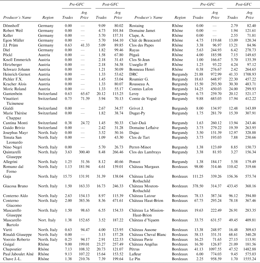
Table 1 lists the name of the wine producers in this study for the three regions and provides descriptive statistics for each. Mixed lots and unsold lots are not considered. All statistics are available for two sub-periods: the (pre-) GFC (01/2002 to 12/2009) and the post-GFC (01/2010 to 12/2017). Generally, Alpine wines are cheaper and less frequently traded than their counterparts from Bordeaux and Burgundy. However, we also observe a significant trend with wines traded more frequently and growing relatively quickly in price since the GFC. In Alpine wine regions, we find differences. The lowest prices and the largest increase in trading activity are in the AGS region. Although there were virtually no trades before and during the GFC, they now have reached levels closer to those of Northern Italy and the Rhône Valley. Prices and trade have also increased in these two regions, but less than for AGS.
Average Price and Number of Trades Per Wine Producer Per Year

Notes: This table reports the average price per year as well as the number of trades recorded in a given year. Mixed lots and unsold lots are not considered. All statistics are available for two sub-periods: pre-GFC (01/2002 to 12/2009) and post-GFC (01/2010 to 03/2018).
IV. Investments in Frontier Assets
We examine the validity of the four propositions. We first examine the evolution of the trading activity of the Alpine wines as compared to two benchmarks, which are Bordeaux and Burgundy. We then estimate indices for Alpine wines and the benchmark regions, and assess their respective performance: raw, real and risk-adjusted returns, total and systematic risk. Finally, we use the estimated indices to analyze the diversification potential offered by each region.
A. Financialization of Alpine Wines
Figure 1 shows the evolution of the trading activity and the average price per bottle for the different regions in 2002, 2010, and 2017. We observe that the number of trades and the average price per bottle fetched at auctions for AGS wines has increased especially after the end of the GFC in 2010 when it was very limited before that. This can be explained by the increase in quality in this region and the efforts of producers to better market wines and become more visible to the public. For instance, several regional and national initiatives have been launched in Switzerland (Mémoire des Vins Suisses, Swiss Fine Wines, rankings, marketing campaigns) and internationally renowned experts have begun to cover their wines and award high scores (several 99/100 in a recent The Wine Advocate article).
Evolution of the Trading Activity and Average Price per Bottle

In Northern Italy it is the Piedmont driving demand and with it trading activity and prices. This region, known by insiders for the past 15–20 years, has now taken the path of Burgundy from two decades ago. Three factors have contributed to this phenomenon. First, it is a region with an immense wine-making tradition, but it is complex and until recently intransparent. The arrival of an expert (Antonio Galloni) has contributed to put it on the map of a broader public and to decomplexify it. Second, consumers want to explore new regions facilitated by the dissemination of information on the Internet. Third, the classic and elegant wine style produced in Piedmont is in line with current consumption trends.
The Rhône Valley, on the other hand, has stagnated. This can be explained by the passion Robert Parker, and consequently many wine drinkers, have displayed for this region's wines since the beginning of the 1990s. This longer dating interest has led to a similar evolution of transactions and values as for the benchmark regions of Bordeaux and Burgundy. In other words, the Rhône Valley is already further on the frontier than AGS and Northern Italy.
Finally, the two more mature wine-growing regions also display a positive evolution. For Bordeaux, it was still well underway until 2010. Since then, volumes and prices seem to have stagnated. In Burgundy, trading activity has only seen a limited increase, but prices have gone up. This is due to the scarcity of bottles in this region, which drove prices up due to a strong increase in demand. It can also be explained by the trend towards a certain style of wine and the fact that Burgundy is closing its current gap with Bordeaux.
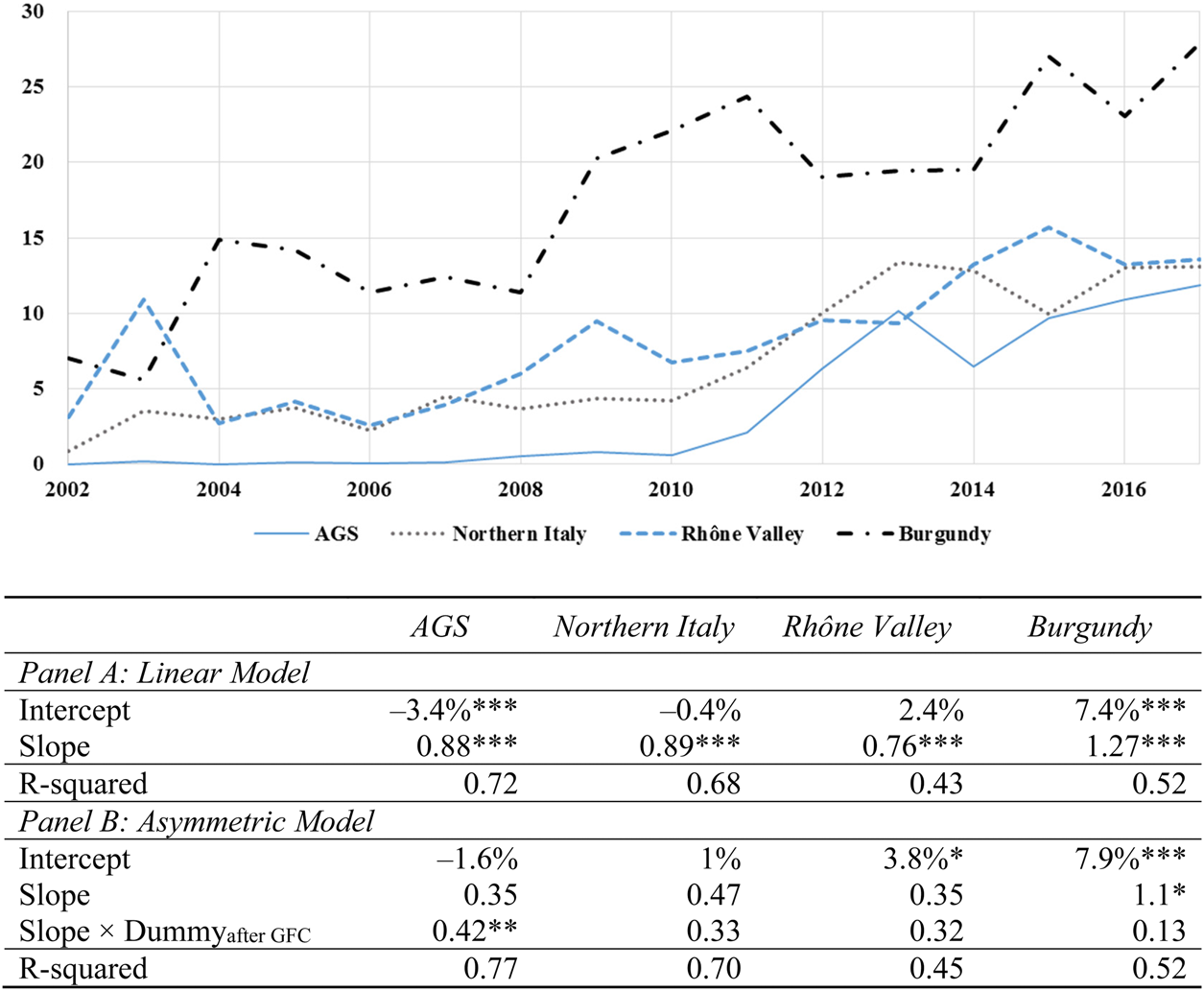
Figure 2 documents the evolution of the trading activity of each wine region compared to Bordeaux. Our findings confirm those reported in Figure 1. Over the entire sample period the importance of Burgundy has strongly increased compared to Bordeaux and now accounts for 30% of Bordeaux trading activity. This is also true for Northern Italy, whereas in the Rhône Valley we observe a slow increase over time. Finally, AGS showed a very limited activity until 2008 and have only truly started to be traded after the GFC in 2010. Over the period 2010 to 2017, it has closed the gap with Northern Italy and the Rhône Valley and all three now account for 15% of Bordeaux trading activity. The graphical evidence is further corroborated by the significant and positive slope coefficients for all regions in a linear model. The strong AGS evolution after the GFC is confirmed in an asymmetric model with a positive and significant slope coefficient which is interacted with a post-GFC dummy.
Evolution of the Trading Activity for Each Region Relatively to Bordeaux (in Percent)

Overall, results in Table 1 and Figures 1 and 2 validate Proposition 1. Alpine wines have followed a financialization process and have slowly caught up with the already investment-grade and financialized regions of Bordeaux and Burgundy.
B. Index Estimation and Analysis
(1) Index Estimation
We estimate indices for Alpine wines and for the two benchmark regions of Bordeaux and Burgundy, using the Repeat-Sales Regression (RSR) approach (Bailey, Muth, and Nourse, Reference Bailey, Muth and Nourse1963). This method has the advantage of not requiring the identification of all relevant price attributes, which is a key advantage over the alternative approach, the Hedonic Regression,Footnote 2 especially in a context in which wines from different regions are considered.
Let p j denote the log price of wine j. Each sale is indexed as follows: t is the time when the first sale took place and τ corresponds to the time when the next sale took place, thus, τ > t. The log-return of wine j between dates t and τ is calculated as r j,t,τ = p j,τ − pj,t. Equation (1) formalizes the RSR approach (see Masset and Weisskopf (Reference Masset and Weisskopf2018b) for details):

where D j,n takes the value 1 if wine j is sold in period τ, –1 if wine j is sold in period t, and 0 otherwise, N is the number of periods in the data sample. We estimate Equation (1) using an OLS specification.Footnote 3 The RSR index is obtained by taking the exponential of the γ n estimates of Equation (1).Footnote 4
(2) Analysis of the Evolution of the Alpine Wine Indices
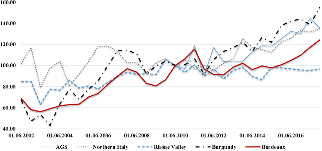
Figure 3 illustrates the evolution of the three Alpine and two benchmark wine indices since 2002 using a bi-annual sampling frequency to reduce the effect of noise and non-synchronous trading activity. We then rescale all index values to 100 at the beginning of 2010, marking the end of the GFC. We observe that wines from Northern Italy and the Rhône Valley showed an essentially flat performance between 2002 and 2009. This contrast with Bordeaux and Burgundy, which saw their value increase by around 50% over the same period. Over the 2010–2017 period, we find that the AGS region performed well with a 40% increase in value. This is in line with findings for Northern Italy and Burgundy and, to a lesser extent, Bordeaux. Finally, the Rhône Valley remained a poor investment and did not create value over this period.
Wine Indices

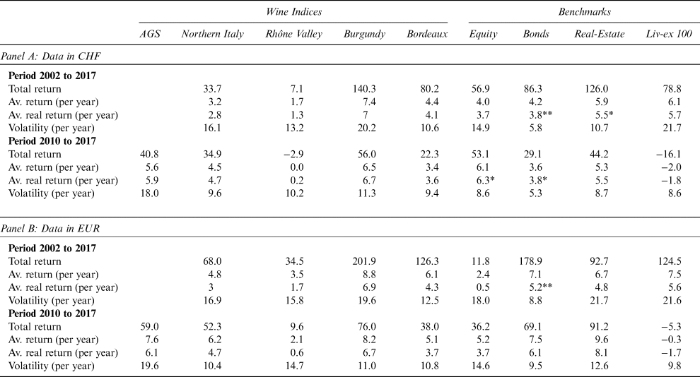
Table 2 presents descriptive statistics on the wine indices and their benchmarks over the entire sample period and the 2010–2017 sub-period. The table is split into two panels: the upper panel considers the indices labelled in their original currency, the Swiss Franc, with Swiss equity, bonds, and real-estate as benchmarks; the lower panel shows Euro indices with equivalent European benchmarks. Given the important fluctuations the Swiss Franc has experienced with respect to the Euro and the fact that most wines are produced in Euro-zone countries (the only exception being Swiss wines), it seems necessary to control for the effect of currency fluctuations on the results. We observe that all assets, except the Liv-ex 100 and the Rhône Valley, have displayed a positive total return for both the entire and restricted sample period. These results also hold once we account for inflation.Footnote 5 As documented, both AGS and Northern Italy have yielded real returns of around 5 to 6% per year. Statistically, the number of observations does not allow us to reject the null hypothesis that average returns are close to zero. However, economically we observe that all our findings indicate strong positive returns throughout the specifications. We therefore consider Proposition 2 is validated and confirms the results for the more financialized regions of Bordeaux and Burgundy, which also have yielded higher returns than the inflation rate, both in CHF and EUR.
Descriptive Statistics on Wine Indices and Benchmarks

Notes: Panel A reports descriptive statistics (in percent) for wine indices expressed in their original currency (CHF), for Swiss equities (Swiss Market Index), bonds (total return index on Swiss government bond), and real-estate (FTSE EPRA/NAREIT Switzerland), as well as the Liv-ex 100 expressed in CHF. Panel B reports similar statistics (in percent), but for wine indices expressed in EUR and benchmark indices of the Euro-zone (Euro Stoxx 50, total return index on Swiss government bond, and FTSE EPRA/NAREIT Europe), as well as the Liv-ex 100 expressed in EUR. AGS stands for Austria, Germany, and Switzerland. For this region, the limited number of observations before GFC implies that only the statistics for the 2010 to 2017 period are reported. Semi-annual data are used to compute the statistics. The asterisks *, **, and *** indicate whether the real rate of returns are significantly different from zero at the 90%, 95%, and 99% level, respectively.
The AGS and Burgundy index show the highest returns, but also the highest volatility. This may be explained by the heterogeneity of the four different regions with a potentially diverse status, ranging from more of a consumer good to a financial asset. Over the entire sampling period, the best performance comes from Burgundy (1st) and Bordeaux (2nd), but if focusing on the more recent period, Burgundy remains the best performer followed by the two frontier regions in Northern Italy and AGS, which all outperform Bordeaux. These observations are in line with the argument that emerging wine regions getting access to the universe of investment-grade wines deliver higher returns. Turning to the Euro-denominated results we find a stronger performance of the wine indices. This is due to the strong appreciation of the Swiss Franc with regard to the Euro during the sample period.
The benchmark indices have mainly performed well. Bonds and real estate have delivered a very strong performance, while equity performed poorly in Europe due to the GFC, the Euro-zone debt crisis, and the ensuing recession. Although this remained true in the Euro-zone for the period 2010–2017, in Switzerland, equities outperformed bonds and real estate after the GFC. Over the entire sampling period, we also found that the wine market benchmark (Liv-Ex) had evolved close to our own Bordeaux index, but much less so during the 2010–2017 period. This can be explained by the composition of the Liv-ex, which includes young wines as opposed to our index and the depreciation of the British poundFootnote 6 since the GFC and the Brexit vote.Footnote 7
C. Risk-Adjusted Returns
(1) Decomposition of the Returns of the Wine Indices
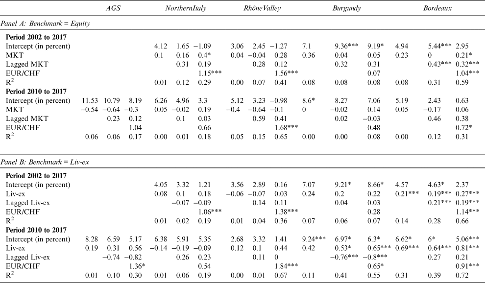
In order to estimate risk-adjusted returns to an investment in Alpine wines and to better understand the drivers of the performance of such an investment, we run two regressions. We first use a CAPM regression with a market risk factor (MKT) (Sharpe, Reference Sharpe1964; Lintner, Reference Lintner1965). This allows us to decompose the returns of Alpine wines into a systematic and a specific component and to determine if these wines have delivered abnormal returns during the sample period. The specification takes the following form:

where R i,t, rf t, and MKT t are the return on index i, the risk-free rate and the market risk factor at time t. β i captures the quantity of systematic risk of index i and α i provides an estimate of its abnormal return. In order to account for nonsynchronicity and a possible delayed reaction of the wine indices, we also consider a specification containing a lagged realization of MKT as defined in Masset and Weisskopf (Reference Masset and Weisskopf2018b),

In a second step, we replace the market risk factor with the return of the Liv-ex 100 index, which is regarded as the industry leading benchmark. The purpose of this second regression is to better understand how Alpine wines react to the general wine market. As before, we also consider a model containing a lagged realization of the excess return of Liv-ex. The specifications are as follows:


where R Liv−ex,t is the return on the Liv-ex 100. The other variables and coefficients are identical to those of Equations (2) and (3). In order to control for the potential effect of exchange rates on our results we also run Specifications (3) and (5), including the variation in the EUR/CHF exchange rate.
(2) Analysis of Risk and Adjusted-Returns
Table 3 presents the results from Specifications [(2)–(3)] and [(4)–(5)] using bi-annual data to limit the impact of non-synchronous trading and noise.
Results from the Single-Factor Regressions

Notes: This table reports the results from three regression models that include, as independent variables, the return to a reference index, the lagged return to this reference index, and the variation in the EUR/CHF exchange rate. Panel A reports the results when the benchmark is the Swiss Market Index and Panel B is for the Liv-ex. AGS stands for Austria, Germany, and Switzerland. For this region, the limited number of observations before GFC implies that only the results for the 2010 to 2017 period are reported. Semi-annual data is used to run the regressions. The asterisks *, **, and *** indicate significance at the 90%, 95% and 99% level, respectively.
Panel A presents results for the Swiss equity market using the Swiss Market Index (SMI) as a benchmark. We observe a low and insignificant beta coefficient for all regions, but for Bordeaux wines, which also holds when we include lagged equity market returns. This indicates that all wine regions, except for the most financialized one, display a different evolution from equity markets and may be interesting from a diversification perspective. The inclusion of the EUR/CHF exchange rate in our specifications does not significantly alter our initial results, but suggests that the exchange rate has a significant and positive relationship with the wine market.Footnote 8 We can interpret the strong CHF as a sign of the economic solidity of Switzerland, which creates a wealth effect and an increase in the purchase of fine wines. Alternatively, a weak EUR is a sign of economic stress in the Euro-zone that leads to the sale of risky assets and the search for safe haven investments such as gold or wine (see Bouri and Roubaud, Reference Bouri and Roubaud2016).
Finally, the alpha coefficient is positive for all indices, but only significantly so for Burgundy and in one Bordeaux specification. These results hold when we restrict our sample to the post-GFC period, with insignificant but low beta coefficients, a significant effect of the EUR/CHF exchange rate and positive, albeit, insignificant alphas. Although not significant, AGS displays strongly positive alphas and negative beta coefficients, hinting at the fact that these regions tend to behave differently than equity markets.
Panel B presents the results with the CHF-translated Liv-ex as a benchmark for the global wine market. This allows us to analyze the segmentation of the wine market. We find that the Bordeaux index evolves similarly to the benchmark index. This may be explained by the composition of our index, which is not only composed of the best wines, but also of less liquid wines from Pomerol and St. Emilion and covers older vintages. Thus, our index is less focused on young, liquid, and speculative wines than the benchmark index and, consequently, displays lower risk estimates. In the post-GFC period, this finding becomes stronger for Bordeaux and Burgundy since these wines start to constitute the majority of trades in our database. More generally, with the exception of Bordeaux, all wine indices are less similar to the overall wine market than to the SMI. This indicates that the overall wine market is still mainly composed of Bordeaux wines and that segmentation continues to exist between wine regions. This is of interest to investors because diversification does not only work in relation to financial markets, but also on the wine market itself. Once again Burgundy displays a strong and positive alpha coefficient confirming the previous results on the strong evolution of this region over the past 15 years and the EUR/CHF exchange rate remains significant. The AGS regions also continues to show insignificant but positive alphas and negative or low beta coefficients. Our findings show the complexity of the wine market for which it is difficult to precisely anticipate the dynamics of the different regions. Once again, we cannot reject the null hypothesis that alpha is equal to zero statistically. However, economically, all our coefficients are large and positive and our specifications show high R2. All these elements hint at an economic validation of Proposition 3 that investment in these frontier markets has led to superior risk-adjusted returns.
D. Diversification Potential and Portfolio Analysis
(1) Portfolio Construction and Diversification Potential
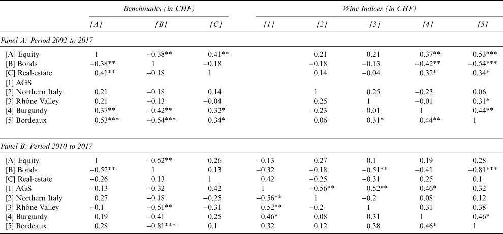
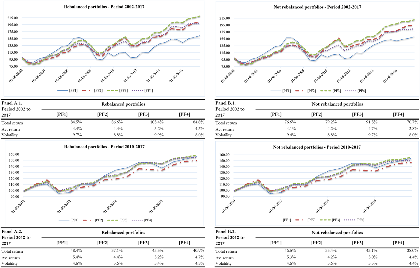
In order to analyze the diversification potential of these wines, we resort to two approaches. First, we perform a correlation analysis to understand the interrelation of different wine regions with each other and with traditional financial markets. This allows us to gauge the segmentation of the wine market and how this translates in a broader investment perspective. Second, we construct different investment portfolios. We are constructing a benchmark portfolio that replicates the traditional strategic portfolio allocation of a rather aggressive investor, who may be interested in investing in wine, consisting of 60% equity, 20% fixed income, and 20% real estate. We then examine the impact of adding 50% wine to this portfolioFootnote 9 by constructing three different wine-invested portfolios. The first has the same structure as the benchmark portfolio, but only invests 50% in the financial assets and 50% in Bordeaux wines. The second portfolio invests 50% of wine equally in Bordeaux and Burgundy. Finally, the last portfolio invests 10% in Bordeaux, Burgundy, and each individual Alpine region. The analysis concentrates on risk and return aspects that are of interest to investors.
(2) Portfolio Analysis
Table 4 presents the results of the correlation analysis of the different financial and wine indices over the period 2002–2017 (Panel A) and 2010–2017 (Panel B). During the complete sample period, we find evidence of three distinct asset categories. The first, with positive correlations of around 0.4, includes the interrelations between equity, real estate, and the two financialized wine markets of Bordeaux and Burgundy. This suggests that the diversification potential that once existed for these two regions has not entirely vanished, but is less pronounced and, thus, reduces their attractiveness in a portfolio setting. The second category displays negative correlations of around –0.4 for the bond market in relation to equities, Bordeaux and Burgundy. Over this period, bonds performed very strongly and constituted the most interesting investment from a diversification perspective. Finally, we have a category with correlations of around 0 for Northern Italy and the Rhône Valley. Although this result is less pronounced than for bonds, both regions nevertheless appear to be of interest for diversification purposes by behaving not only differently from traditional financial assets, but also from more financialized wine regions. This further confirms the existing segmentation in the wine market. The period 2010 to 2017 yields similar results, with bonds being negatively correlated with equities, Bordeaux and Burgundy. Also these two regions remain positively correlated with equity and real estate, but slightly less than over the entire sample period. This is due to the different evolution of equity and Bordeaux prices, with the first dropping during the GFC and the second in 2010–2011. Finally, the AGS region displays correlations of around 0 and appear equally interesting for diversification as its Northern Italian and Rhône Valley counterparts.
Correlation between Wine Indices and Benchmark Assets

Notes: This table reports the correlation among the various indices. Panel A reports the results from the complete sample period and Panel B considers only the period 2010 to 2017 (i.e., the period after GFC). AGS stands for Austria, Germany, and Switzerland. For this region, the limited number of observations before GFC implies that only the results for the 2010 to 2017 period are reported. Semi-annual data is used to compute the correlations. The asterisks *, **, and *** indicate significance at the 90%, 95%, and 99% level, respectively.
To further investigate the performance of frontier assets, we resort to the construction of portfolios in order to judge the potential of this type of investment in a traditional financial portfolio. We once again perform computations over the entire sample period (2002–2017) and the restricted period (2010–2017) and report the results in Figure 4.
Portfolios

Over the entire sample period, we observe that adding Bordeaux and Burgundy wines to a financial portfolio led to a 15 to 20% increase in returns, but also to a slightly higher volatility. Only adding Bordeaux was less interesting, showing that it has been especially Burgundy wines that have driven performance during this period. Finally, we find evidence that investing in both financialized and frontier wine regions led to a similar return, but slightly lower risk as compared to only investing in financial assets. Results on the restricted period between 2010 and 2017 depict a different outcome. During this period, including Bordeaux wine in a portfolio was a poor choice, leading to lower returns and an increase in risk. This is due to the bursting of the Lafite Rothschild bubble between 2011 and 2015 during which Bordeaux wines lost up to 60% of their value. This could have been counterbalanced by investing a portion of the funds in Burgundy, which has greatly gained in consumer and investor favor during this period. Finally, adding frontier wines has led to an increase in returns and lowering of risk compared to an investment in Bordeaux only. More generally, frontier wines have not been able to improve portfolio returns. Nevertheless, they allowed for a decrease in portfolio risk because of their low volatilities and correlations with traditional assets and the Bordeaux and Burgundy region. It, thus, appears that identifying the new frontier markets at the right time leads to valuable outcomes for investors validating Proposition 4.
V. Analysis and Practical Implications
This section responds to four questions that analyze the practical implications of our findings and also discuss certain risks and limitations associated with an investment in frontier assets.
Why include these assets in a portfolio? Generally, the inclusion of an asset in a portfolio is motivated by high returns, a low risk, and/or a low correlation with other assets. Our analysis suggests that these three elements are united in the case of Alpine wines. However, this conclusion needs to be mitigated due to statistical reasons: our sample is limited in terms of observations and covers a period of less than 20 years. The findings are therefore specific to this period. In addition, returns (which are less sensitive to a low number of observations) are estimated more precisely, which makes them more robust and reliable. We, thus, in terms of performance, find strong support that frontier assets deliver higher returns. For the volatility and correlation (which are sensitive to the methodological choices considered, and, among other things, the sample frequency), we also find results that are clear and economically consistent, but need to be interpreted with more care.
How to identify these assets? The wines close to the frontier are specific in the sense that these are initially single wines produced by reputable winemakers, who place themselves close to the frontier. Then, gradually, other winemakers in the region gain access to this status and put the entire region on the investment map. This happened in Burgundy two decades ago, and more recently, in the French Jura. Before being on the frontier, these assets were known to wine amateurs but were rarely traded on the secondary market. With the gradual increase in reputation and status, first collectors and then investors were attracted. Wines started to be more and more traded and their price began to increase. The element to identify such assets is, consequently, the moment when they begin to represent a significant activity in the secondary market. Many wines, and not only from the Alpine regions, have followed this path over the past few years. For example, some wines from the Loire valley (e.g., the Clos Rougeard has seen its prices multiplied by ten over the last decade), the Chablis (Dauvissat and Raveneau), the Languedoc (Granges des Peres), and increasingly wines from the New World.
For whom? The discussion earlier suggests that these investments are destined for insiders who have already exhausted the performance and diversification opportunities offered by more traditional asset classes. A good knowledge of the wine market and its specificities as well as a certain capacity to take risks are also essential. Unlike Bordeaux wines in which one can invest via wine funds, there are, for the moment, no satisfying solutions for outsourcing the management of a frontier wine portfolio.
What to pay attention to? An investment in frontier wines/assets presents risks in the asset class, but also in the individual selection of the asset. At the macro level, the current environment (high liquidity on markets, traditional assets with rather weak perspectives, and strong growth of potential new clients especially from Asia) is very favorable for this type of asset. This configuration will, however, not last forever. It is, thus, possible that frontier wines/assets will lose interest at some point in time. Frontier assets are not only risky in terms of their volatility, but also because of their restrained liquidity. Our study suggests that other variables, such as the exchange rate, are also significant. Finally, one has to consider that many wines have appeared to approach the frontier in the past (impeccable quality and progressive increase of secondary market activity), but they have never seen their price rise. Sauternes wines are probably the best example: their quality remains at the top, but demand is rather low, leading to stagnating or dropping prices over the last ten years.
VI. Conclusion
John F. Kennedy stated that “we stand today on the edge of a new frontier - the frontier of the 1960's - a frontier of unknown opportunities and perils - a frontier of unfulfilled hopes and threats.” Humans have always tried to expand frontiers and to go beyond existing or known boundaries. In this article, we investigate another type of frontier: the frontier of investable assets. Following the GFC, excess liquidity in the markets, due to low interest rates and quantitative easing, has driven prices of traditional financial assets and of alternative assets upwards. As a consequence, investors have started to push the frontier of investable assets even further to invest their funds profitably. Today we are in an area that can be classified as a frontier of alternative alternatives.
Using the market for fine wine as a setting, we propose and test four propositions related to last frontier investments composed of Alpine wines. We compare our results with both traditional financial assets and the already financialized wine regions of Bordeaux and Burgundy. We show that Alpine wines at the frontier between consumer goods and financial assets are increasingly popular since the GFC and have seen their number of trades and values strongly increase. This has led prices of Alpine wines to increase faster than inflation rates. We further find evidence that Alpine wines have delivered positive risk-adjusted returns and strong diversification benefits in the context of financial portfolios. Overall, pursuing frontier investments and taking a position on the edge of investable assets has been beneficial for investors over the last decade.