


Introduction
Floating ice shelves along the coast of North Greenland and around the periphery of Antarctica undergo a continuous cyclic vertical motion forced by oceanic tides (Reference HoldsworthHoldsworth, 1969, Reference Holdsworth1977). Most of the differential motion caused by oceanic tides is accommodated over a few km-wide band at the transition between grounded and floating ice called the tidal flexure zone. This narrow zone is the site of important glaciological processes, which include cyclic bending and cracking at tidal frequencies, transmission of longitudinal stress gradients across the grounding line, and transition in flow style between ice-sheet mechanics and ice-shelf dynamics.
Tidal flexing has been studied with tiltmeters (Reference RobinRobin, 1958; Reference StephensonStephenson, 1984; Reference SmithSmith, 1991), kinematic global positioning system (GPS) (Reference VaughanVaughan, 1994; Reference Reeh, Mayer, Olesen, Christensen and ThomsenReeh and others, 2000) and interferometric synthetic aperture radar (InSAR) (Reference Goldstein, Engelhardt, Kamb and FrolichGoldstein and others, 1993; Reference RignotRignot, 1996). InSAR offers greater precision than other methods (see Reference RignotRignot, 1998c, for a comparison with GPS) and is the only method that provides snapshots of the differential tidal displacement of an ice shelf, simultaneously, at a high spatial resolution (20m), over extensive areas (100 km). With quadruple difference InSAR, it is possible to precisely locate grounding lines (Reference RignotRignot, 1996), detect grounding-line migration with time (Reference RignotRignot, 1998a, Reference Rignotb, Reference Rignotc) and changes in ephemeral grounding (Reference Schmeltz, Rignot and MacAyealSchmeltz and others, 2001), which have important implications for the study of the mass balance of an ice sheet.
Several authors have compared measurements of tidal bending along a profile with model predictions of an elastic beam of ice (Reference HoldsworthHoldsworth, 1969; Reference VaughanVaughan, 1995; Reference RignotRignot, 1996). The one-dimensional elastic model, with a tuned value of Young’s modulus of ice, can reproduce observed data fairly well. Furthermore, Reference VaughanVaughan (1995) showed that most glacial tidal bending zones could be modeled with a value of E about 0.88 ± 0.35 GPa.
In this study, we compare InSAR observations of tidal bending with model predictions from an elastic plate of a variable thickness, hence a two-dimensional model of elastic bending, with a varying ice thickness. The model is first validated using computer-generated data for which an analytical solution is available. A forward model approach is then employed to compare model predictionswith InSAR observations. Two examples from Antarctica are analyzed. A detailed analysis of the time variability of the results is then conducted on Pine Island Glacier, West Antarctica, and Petermann Gletscher, North Greenland, using multi-year InSAR observations. We conclude by assessing the applicability of the elastic bending model to real situations.
2. Two-Dimensional Elastic Bending
The deformation of an elastic beam of ice was discussed by Reference HoldsworthHoldsworth (1969, Reference Holdsworth1977). From the more general case of the equilibrium of plates (e.g. Landau and Lifshitz, 1970), the deformation of a beam of variable flexural rigidity, supported by ocean waters underneath, may be written as (simplified equation in Reference HetényiHetényi, 1946, p. 99)

▽ is the gradient operator  x; y are the horizontal axis, η is the vertical displacement, ρw is the density of sea water, g is the acceleration of gravity, T is the tidal amplitude, and D is the flexural rigidity of ice, defined as
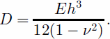
E is the elastic (Young’s) modulus, ν is Poisson’s ratio, and h is ice thickness.
The dimensions of the ice shelves considered in this study are greater than their thickness, so they may be considered semi-infinite slabs. The horizontal displacement due to tidal bending is neglected, as well as the vertical shear stress gradient.
The bending stress generated at the grounding line at the surface and calculated from the analytic solution of the elastic-beam theory for a semi-infinite slab is (Reference HoldsworthHoldsworth, 1969; Reference HughesHughes, 1977):
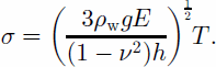
With an average thickness of 1000m at the grounding line and E = 3 GPa, we obtain for Pine Island Glacier σ = 1.6 bar for a deflection of 50 cm. The same calculation for Petermann Gletscher (thickness 600 m) gives σ = 2 bar. These values are within the limits of the elastic theory (σ<2 bar; Reference Budd and JackaBudd and Jacka, 1989). However, the tidal amplitude reaches 80 cm in the Pine Island area and 90 cm for Petermann Gletscher, so that at high tide the bending stress may exceed the elastic limit. The use of the elastic theory is therefore justified for small deflections (550 cm). For large displacements, observations must be compared with the elastic bending theory to determine whether the deformation is still elastic.
Following Reference HoldsworthHoldsworth (1969), we impose the limit conditions:

(3a) means that there is no vertical displacement along the hinge line, and the slope is zero, and (3b) means that the vertical displacement is equal to the ocean tide at the ice front, with zero slope.
We define an elastic damping factor, βe, as

To solve Equation (1) numerically, we operate a change in variable

The differential equation of fourth degree with one unknown (Equation (1)) is replaced by a non-linear system of two equations of degree two with two unknowns
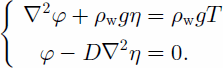
This system is solved using a variational approach for η and φ. The model is implemented using Mat Lab (www. mathworks.com), and the finite-element meshing is generated using Argus (www.argusint.com), with the geometry of ice shelves observed in European Remote-sensing Satellite (ERS) imagery.
3. Results
3.1. Perfectly rectangular slab of ice of uniform thickness
To test the elastic model, we compare its output with an analytical solution (Reference HoldsworthHoldsworth, 1969) in the case of a finite-length beam of ice of rectangular dimensions. The beam is 30 kmwide, 1.5 km thick and 100 km long. The elastic modulus of ice is E = 0.88 GPa (Reference VaughanVaughan, 1995); the Poisson ratio is ν = 0.3 (as in the rest of the paper); ρw = 1030 kgm–3, and g = 9.81ms–2. The hinge line, where the beam is rigidly anchored to the ground, is positioned at x = 0. The tidal amplitude is T =1m. The wavelength number βe –1 is 3.2 km. The spacing between mesh nodes is 1km on average, and 500 m in the vicinity of the hinge line (x =0). Figure 1 shows the vertical displacement of the beam along the center line (y =15 km). We see that tidal bending is concentrated in a region about 8 km wide, and reaches an extremum before converging to an asymptotic value that corresponds to the ocean tide.
(a) Modelled tidal flexure for a rectangular plate of constant thickness (solid line) and varying thickness (dashed line); (b) model solution minus analytical solution for the case of constant thickness (solid line) and varying thickness (dashed line).
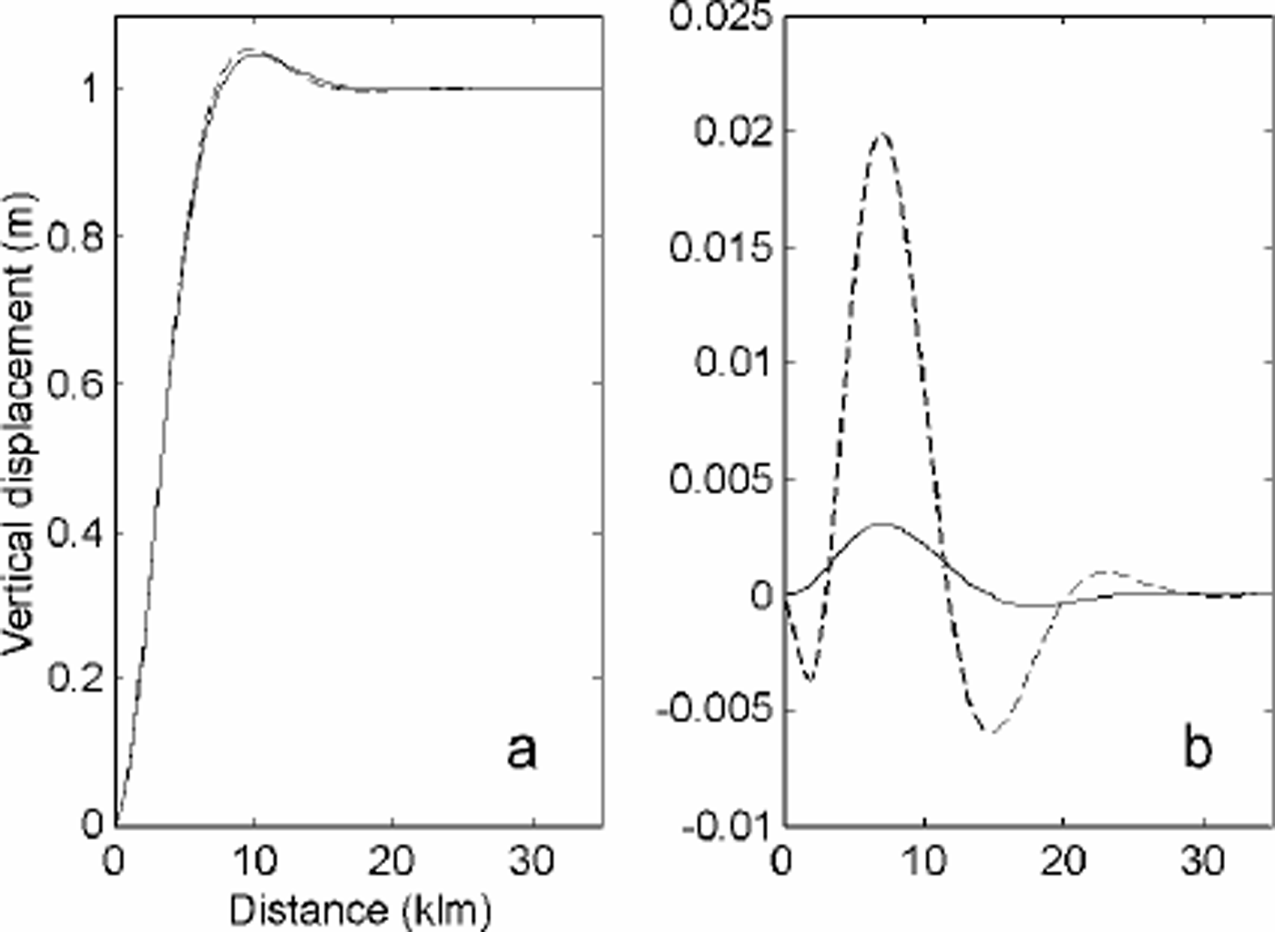
In this simple situation, the agreement between model and simulation is 0.35% (or 3.5 mm in this case for a tide of 1 m), which is probably of the order of precision of the numerical results.
3.2. Perfectly rectangular slab of ice of varying thickness
The thickness of glaciers typically decreases rapidly downstream of the grounding line. This pattern was interpreted as plastic necking by Reference HoldsworthHoldsworth (1977), or evidence of basal melting by Reference RobinRobin (1958). Plastic necking may be of importance when basal friction is significant upstream of the grounding line, and the glacier velocity at the bed needs to adjust to the surface velocity as basal drag becomes negligible on the ice shelf. In the case of more active outlet glaciers, however, basal sliding velocities are already close to surface velocities, and plastic necking is presumably negligible. The gradient in ice thickness is then due to a combination of basal melting and ice-shelf lateral spreading. Basal melting is most intense near the grounding zone since this is where the ice draft reaches the greatest depth and the pressure-dependent melting point of ice is the lowest.
We simulate the effect of a thickness gradient by using a rectangular plate of linearly decaying thickness in the along-flow direction, at a rate corresponding to a basal melt rate of 50ma–1 and a glacier velocity of 2.5 kma–1 (typical of Pine Island Glacier: Reference RignotRignot, 1998a). The thickness slope is thus 2%. On Petermann Gletscher, basal melting is 24ma–1 in the vicinity of the grounding line, ice flows at 1.2 kma–1, and the thickness slope, again, is 2%( Reference Rignot, Krabill, Gogineni and JoughinRignot and others, 2001).
The model simulation for a plate of varying thickness is compared with the analytical solution for a plate of fixed thickness (equal to the glacier thickness at the hinge line) in Figure 1. The result shows that the thickness gradient does affect the bending of ice. The flexure zone is narrower by about 1km and the two profiles differ by up to 2%. The effect of a thickness gradient is therefore small, but not
negligible. We expect many glaciers to exhibit a thickness gradient comparable to those employed here. Detailed comparisons of InSAR observations with an elastic model of tidal bending therefore ought to incorporate the effect of a varying ice thickness if a modelling precision better than a few per cent is expected.
3.3 Effect of grounding-line migration
The vertical displacement measured in a tidal interferogram is not a direct expression of the displacement due to tide. It is a difference in tidal displacement recorded between different dates, hence at different tides (Reference Rignot, Padman, MacAyeal and SchmeltzRignot and others, 2000). As the ocean tide goes up and down, the point of contact of the glacier will move back and forth with high tide or low tide. This effect may be large if the bed slope is small. This migration introduces non-linearities in our model.
To investigate the effect of grounding-line migration on tidal modelling, we did the following simulation. We use a semi-infinite beam, 1000m thick, with a thickness slope of 1% at the grounding line, and E =1GPa. At zero tide, the grounding line is at x = 0. At high tide (T = 1m), the grounding line retreats to x = –100m. At low tide (T = –1m), the grounding line advances to x = +100m. The difference in tidal displacement between low and high tide is, so to speak, equivalent to what would be measured in a tidal interferogram between the two epochs. The mean position of the grounding line between the two epochs should be x = 0m. Using model fitting on the difference (the differential vertical displacement is then 2m), we infer a grounding-line position at x = 0, with E =1.01GPa. Hence, the mean grounding-line position is estimated accurately, but E is estimated with a 1% error. This error is small, however, so in the rest of the study we assume that the migration of the grounding line with tide does not have a significant impact on model fitting. This is equivalent to assuming that the grounding line is rigidly anchored at x = 0, which is the mean-sea-level position of the grounding line.
3.4. Pine Island Glacier, West Antarctica
Pine Island Glacier is a fast-moving outlet glacier which develops a 50 km long ice shelf in the Amundsen Sea, West Antarctica. Its sinuous grounding-line profile is shown in Figure 2, at the outer blue-colored boundary of the model domain (Reference RignotRignot, 1998a). The thickness data used in the model combine ice-shelf elevation from Reference Bamber and BindschadlerBamber and Bindschadler’s (1997) digital elevation model (DEM) of Antarctica at 5km spacing, and ice-sounding radar measurements collected by the British Antarctic Survey (BAS) (Reference Corr, Vaughan, Doake and JenkinsCorr and others, 2000). The data are interpolated between grounded and floating ice using a triangle-based cubic interpolation in MatLab which insures a smooth transition in ice thickness between the two domains. In our mesh, the spacing between nodes is 3.5 km, decreasing to 1.3 kmin the vicinity of the grounding line.
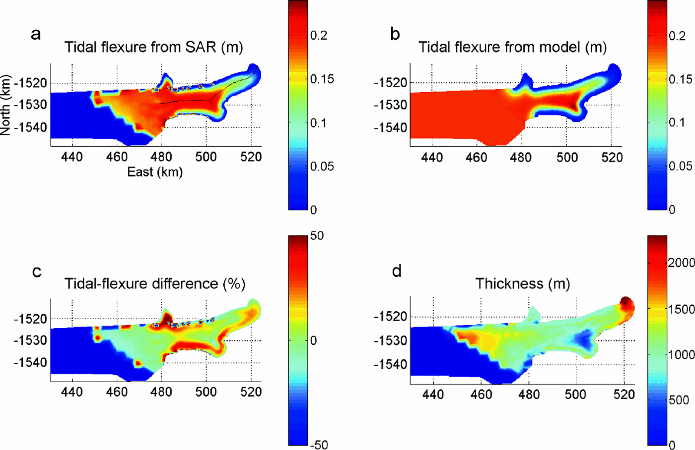
Tidal flexure (in m) on the floating part of Pine Island Glacier, observed with InSAR (a) and modelled with an elastic plate of varying thickness (b), and difference between InSAR and the model in reference to InSAR in per cent (c). (d) The thickness map used in the model. Coordinates are in km on a polar stereographic grid.

The two orbit pairs used to generate the first tidal interferogramare 23627/3954 (ERS-1/-2) and 24128/4455 (ERS-1/2). The tidal displacement is 35 cm. Two values of E are tested: 0.88 GPa (Reference VaughanVaughan, 1995) and 3 GPa (Reference RignotRignot, 1996), which encompass the minimum and maximum values quoted in the literature (e.g. 1.1–1.8GPa for Reference SmithSmith, 1991; 2.7 GPa for Reference HoldsworthHoldsworth, 1969, Reference Holdsworth1977).
Comparison of the model results with InSAR shows good agreement for the main characteristics of the grounding line (maximum vertical displacement, length of the flexure zone), and regions of extending or contracting grounding zone (sinuous contours) where two-dimensional effects are important. Figure 2 shows the comparison for E =0.88 GPa. Areas where the model output and InSAR differ include: (1) zones of partial grounding (i.e. which do not display the full range of tidal displacement because the ice shelf is only grounded at low tide); and (2) areas where the map of ice thickness is less reliable.
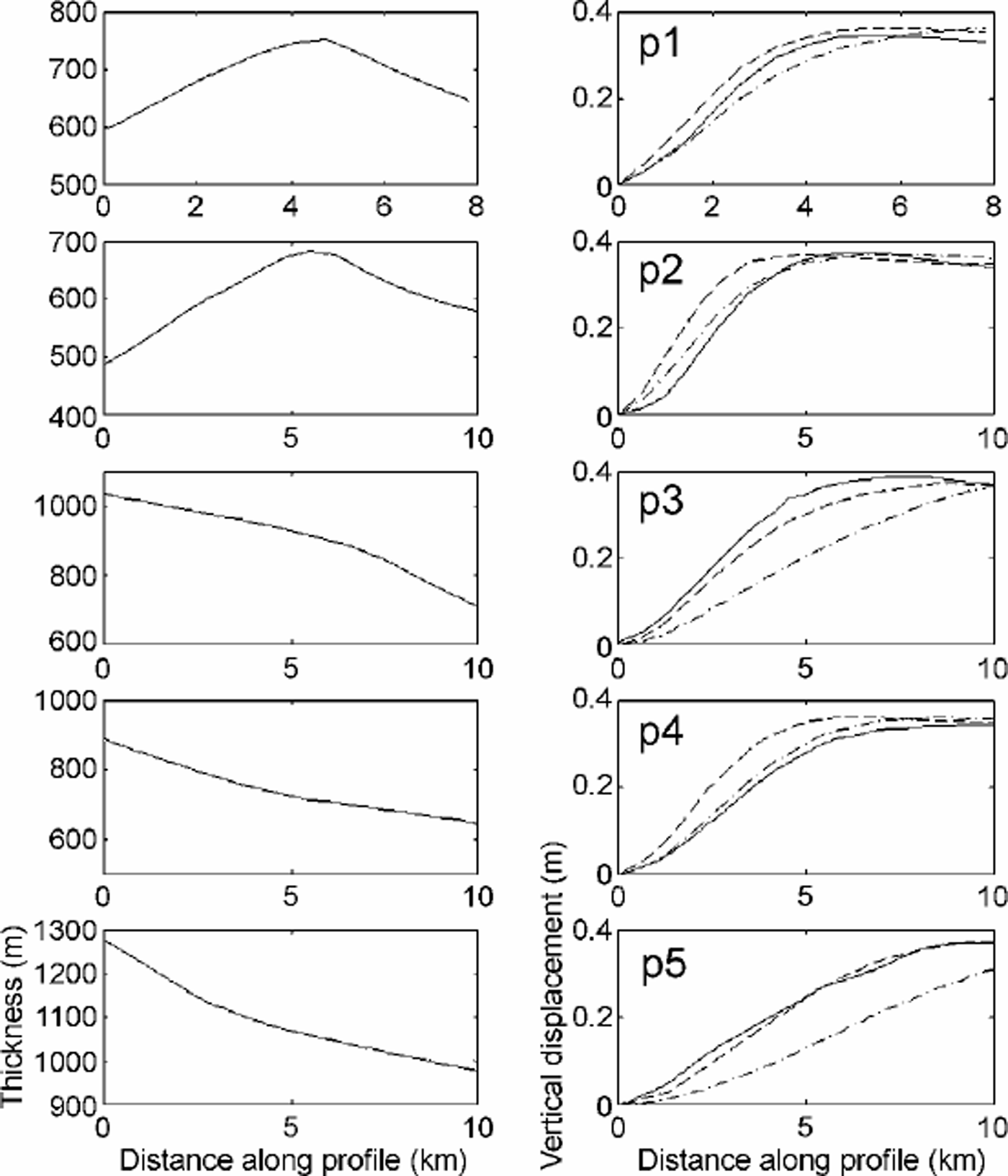
For a more detailed comparison, we extracted several profiles (p1–p5 in Fig. 2a) in a direction perpendicular to the grounding line, and compared the vertical displacement from InSAR and the model for E = 0.88 GPa and E = 3 GPa. The results in Figure 3 show that the same Young’s modulus does not fit all profiles. The precision in ice thickness is one limiting factor. For a given flexural rigidity of ice, a 10% uncertainty in thickness yields a 40% uncertainty in E. The pattern of flexure is also distorted in places where crevasses and bumps and hollows in surface topography are present.
Comparison along the profiles, p1–p5 (Fig. 2). Left: thickness along each profile, in m; right: vertical displacement along each profile, in m, from InSAR (solid line) and from the two-dimensional elastic-plate model with E =0.88 GPa (dashed line) or with E =3 GPa (dot-dashed line).
In Figure 4, we compare a profile along the BAS transect (profile A in Fig. 2). This profile is not perpendicular to the grounding line, but provides a comparison between our thickness map and observation. The standard deviation is 96 m. The best data fit is obtained for E = 0.88 GPa on this profile.
(a) Thickness along traverse A (Fig. 2) measured with radio-echo sounding (solid line) and extracted from our thickness map (dashed line); (b) tidal flexure from In-SAR (solid line),and from the two-dimensional elastic-plate model with E =0.88 GPa (dashed line) or E =3 GPa (dot-dashed line).
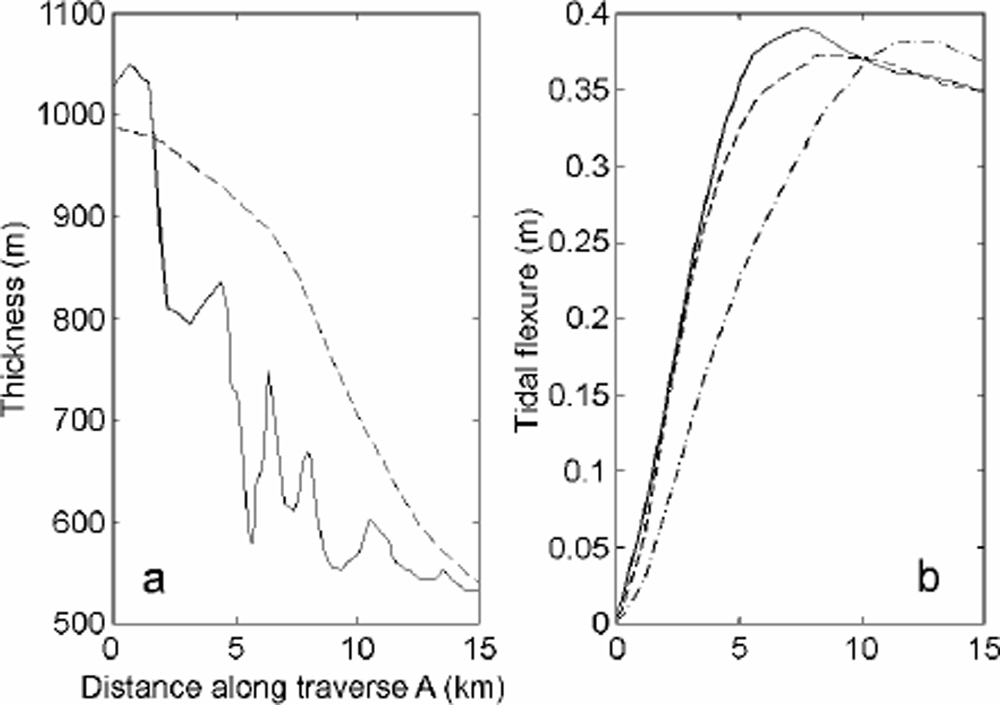
This example shows that a simple elastic-plate model is able to reproduce the main pattern of tidal bending, the sinuous contours of a grounding line, provided that ice thickness is reasonably accurate.
3.5. Drygalski Ice Tongue, East Antarctica
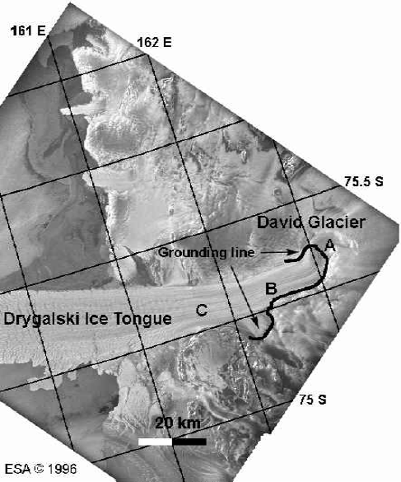
David Glacier is the largest outlet glacier in Victoria Land, Antarctica. It develops into the Drygalski IceTongue, which extends 100 km into the ocean (Fig. 5). David Glacier flows down a deep subglacial trough (Reference SwithinbankSwithinbank, 1988). The grounding line was initially positioned at C (Fig. 5) by Reference FrezzottiFrezzotti (1993) and later revised to B (Fig. 5) by Reference Frezzotti, Tabacco and ZirizzottiFrezzotti and others (2000) based on GPS data. No GPS data were collected upstream of location B. InSAR places the grounding line at point A (Fig. 5) (Reference RignotRignot, 2002), which is 15 km upstream of the position suggested by GPS. The zone of tidal flexure along the glacier center line stretches over 30 km, rather than the usual 8–10 km.
ERS amplitude image of David Glacier and Drygalski Ice Tongue on a polar stereographic grid. The grounding line inferred from InSAR is shown in black, thick line. Points A–C are discussed in the text.
Ice thickness on Drygalski IceTongue may be estimated from surface elevation. Because of the presence of numerous mountain peaks in the vicinity of the glacier, satellite radar altimetry data are not reliable in that sector. Instead, we employed a topographic map generated from InSAR, with a vertical precision no better than 20 m. From this map, the glacier thickness is estimated to exceed 3000 m at the grounding line, and to decrease rapidly toward the ice front. No direct measurement of ice thickness exists close to the InSAR grounding line to confirm our estimate (personal communication from M. Frezzotti 2000). The thickness estimate near B is, however, consistent with ice-sounding profiles described by Reference Frezzotti, Tabacco and ZirizzottiFrezzotti and others (2000).
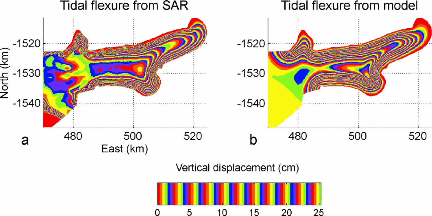
Using the InSAR-derived thickness, we obtain a reasonable fit between InSAR observations and model predictions, using E = 1GPa and a tidal forcing of 19 cm (Fig. 6), especially on the center line (Fig.7), for the length of the flexure zone and the vertical displacement. The agreement is poorer on the sides. The comparison between model and InSAR is shown in more detail in Figure 8, with a zoom on the eastern part. Model simulations that employ a constant or lower ice thickness improve the agreement on the sides, but fail to reproduce the observed tidal pattern along the center line where the tidal flexure extends over a large distance. The unusual stretching of the flexure zone results from tidal bending along the glacier sides (where ice is thinner than at the glacier center according to InSAR), combined with tidal bending in the longitudinal direction where a pronounced ice-thickness gradient exists (Reference RignotRignot, 2002).
Same as Figure 2 for David Glacier.
Comparison between InSAR and model along the profile shown in Figure 6. (a) Thickness along the profile (extracted from our thickness map); (b) vertical displacement along the profile, from InSAR (solid black line), and extracted from two-dimensional model (dashed red line).

Tidal deformation in the vicinity of the grounding line of David Glacier, using (a) an elastic-plate model and (b) InSAR.
3.6. Non-elastic behavior
There is no general agreement on the value of E to be used in model simulations of tidal bending, or on the effective thickness to be used in the calculation since bottom and surface crevasses generated by tensile stresses at the bottom and top surfaces of the glacier may reduce the effective thickness of the ice slab that undergoes tidal flexing (Reference Lingle, Hughes and KollmeyerLingle and others, 1981). Reference DoakeDoake (1978) suggested that flexing of ice shelves may represent 30% of global tidal dissipation, while Reference VaughanVaughan (1995) argued that most glacier data fit a model with E = 0.88 ±0.35 GPa using the full thickness of the ice slab, and hence tidal dissipation is unlikely. Reference RignotRignot (1996) found that a higher value of E (3±0.2GPa) was required to fit InSAR observations of Petermann Gletscher.
Notes: The pairs of ERS-1 and -2 orbits used to detect the grounding line are listed in the second column. H is the glacier thickness at the grounding line along profile p3, p4 or p5 (Fig. 2), or along the center line of Petermann Gletscher (Reference RignotRignot, 1996), inm. E is the elastic modulus inferred from model fitting, in GPa. ηmax is the maximum differential displacement recorded along the profile, in cm.
The reason for the lack of agreement between the various inversions may be that ice does not deform elastically. Reference Reeh, Mayer, Olesen, Christensen and ThomsenReeh and others (2000) reached that conclusion as they observed a time delay of about 35 min between the tidal cycle and the ice-shelf response in northeast Greenland. Such a time delay is not explained by the elastic theory.
One way to detect non-elastic behavior of tidal bending of ice is to examine the temporal evolution of the pattern of tidal bending. This may be done using InSAR on different dates. If the deformation is elastic, a model inversion should yield the same value of E, within errors, because ice thickness does not change.
Table 1 shows the results of model inversions performed on Pine Island Glacier and Petermann Gletscher (one-dimensional model fitting, along profiles perpendicular to the grounding line). The bottom row of Table 1 corresponds to the result published by Reference RignotRignot (1996), with a high value of E, for Petermann Gletscher, using ERS data collected by ERS-1 in 1992 during a 3 day repeat cycle of the satellite. Ice thickness is constrained on all four profiles by ice-sounding radar measurements. Profiles p3–p5 are shown in Figure 2. The profile on Petermann Gletscher runs down the center of the glacier.
Model inversion of the pattern of tidal flexure of polar glaciers observed with InSAR
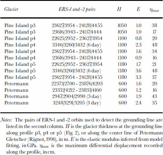
On profile p4, E varies between 0.8 and 2.3 GPa, i.e. a factor three. The largest value is obtained for ERS data acquired in 1992, when the satellite revisit period was 6 days and hence the glacier experienced the largest changes in tide from one satellite pass to the next, as revealed by the maximum value of the tidal bending (last column of Table 1). The same conclusion is obtained on profile p5, with E varying between 1.7 and 3.6 GPa. Even with 1day separation ERS data, the inferred value of E varies by a factor two. On profile p3, we do not observe such variation with tide, however, and the inferred values of E are lower on average.
On Petermann Gletscher, E varies between 1.2 and 2.4 GPa, and the highest values are again obtained when the glacier experiences the largest changes in tide between successive passes of the satellite.
Overall, E must vary between 0.8 and 3.5 GPa in order to best fit the InSAR observations. This result conflicts with the elastic theory. It cannot be attributed to grounding-line migration with tide as discussed earlier. It is also well beyond measurement errors (2%).
Reference HoldsworthHoldsworth (1977) and Reference HughesHughes (1977) examined more comprehensive mechanical models of tidal bending of ice shelves that include viscous, plastic and primary creep processes. Their analysis recognized that although the curve of elastic deformation fits well with observations, the parameter βe to be used in the model is generally smaller than that predicted by the elastic theory. The explanation is that visco-plastic effects tend to delay the ice-shelf response, or resist the action of ocean tides, resulting in an apparent increase in the rigidity of ice during tidal flexing, and hence a lower value of βe. As a result, values of E inferred from an elastic model tend to be higher than predicted.
Conclusions
A simple elastic-platemodel of varying thickness is capable of explaining the major characteristics of InSAR observations of tidal flexing along ice-sheetmargins. It is also able to replicate the unusual tidal bending of David Glacier flexure zone along the center line. Model simulations, however, show that the thickness gradient characteristic of many large outlet glaciers in Antarctica and Greenland has a detectable effect on the pattern of tidal bending. The precision in ice thickness and thickness gradient is an important limiting factor for the two-dimensional modelling. Furthermore, a detailed analysis of temporal variations in tidal bending suggests that the value of Young’s modulus of ice to be used in elastic models must vary with tide, which is in violation of the elastic theory. Although the shape of the tidal deformation is well described by the elastic model, the elastic properties of ice are ill-observed. This suggests that visco-plastic effects must be included in the model. The same conclusion was reached by Reference Reeh, Mayer, Olesen, Christensen and ThomsenReeh and others (2000) from measurements of the time delay between tidal forcing and ice-shelf response. Our examination of InSAR analysis supports their result. Initially, we may expect these non-linearities to be small since the observed deformation is within the elastic regime. Yet this is not confirmed by observation. One consequence of this is that the conclusion that ice-shelf tidal deformation is not dissipative should be revisited. A more detailed study of the variability of E with time will be pursued in future research.
Acknowledgements
This work was performed at the Jet Propulsion Laboratory, California Institute of Technology, under a contract with the National Aeronautics and Space Administration, Cryospheric Sciences Program. We thank the European Space Agency, the VECTRA project and Alaska SAR Facility for distributing the radar data employed in this study. We also thank G. Peltzer for insightful discussions, H. Corr for making the ice-thickness data of Pine Island Glacier available to us, and two anonymous reviewers whose comments were very helpful in clarifying the manuscript and fixing some modelling issues.



