1 Introduction
In the past three decades, a great deal of interest has been evoked in obtaining efficient schemes for the numerical solution of a system of ordinary differential equations (ODEs)
 $$ \begin{align} \begin{array}{l} y^{\prime}(x) = f(x,y(x)),\quad x\in[x_{0},\overline{x}],\\[3pt] y(x_{0})= y_{0}, \end{array} \end{align} $$
where
 $f:[x_{0},\overline {x}]\times \mathbb {R}^{m}\rightarrow \mathbb {R}^{m}$
and m stands for the dimension of the system. As a unifying structure for the most prevalent multivalue and multistage methods, general linear methods (GLMs) were introduced by Butcher [Reference Butcher14, Reference Butcher15]. The explicit GLMs with good properties in accuracy and stability have been recently investigated and constructed in the literature [Reference Bartoszewski and Jackiewicz12, Reference Butcher and Jackiewicz18, Reference Butcher and Wright19, Reference Chollom and Jackiewicz23, Reference Jackiewicz29, Reference Jackiewicz and Tracogna30–Reference Jackiewicz and Verner32, Reference Wright37, Reference Wright38]. Due to the benefits of the class of second derivative methods [Reference Cash21, Reference Chan and Tsai22, Reference Enright27, Reference Hojjati, Rahimi Ardabili and Hosseini28], to obtain methods with high order accuracy and good stability properties, GLMs were extended to second derivative general linear methods (SGLMs) by Butcher and Hojjati [Reference Butcher and Hojjati17]. This large family of methods has been widely analysed and successfully implemented on various time-dependent problems [Reference Abdi1–Reference Abdi and Hojjati7, Reference Movahedinejad, Hojjati and Abdi34, Reference Movahedinejad, Hojjati and Abdi35]. These methods are characterized by p and q respectively as the order and stage order, r as the number of external stages, s as the number of internal stages, the abscissa vector
 $c=[c_{1} c_{2} \ldots c_{s}]^{T}$
and the coefficients matrices
 $$ \begin{align*} \begin{array}{@{}c@{}} A=[a_{ij}]\in\mathbb{R}^{s\times s},\quad \overline{A}=[\overline{a}_{ij}]\in\mathbb{R}^{s\times s},\quad U=[u_{ij}]\in\mathbb{R}^{s\times r},\\[6pt] B=[b_{ij}]\in\mathbb{R}^{r\times s}, \quad \overline{B}=[\overline{b}_{ij}]\in\mathbb{R}^{r\times s},\quad V=[v_{ij}]\in\mathbb{R}^{r\times r}. \end{array} \end{align*} $$
SGLMs, on the uniform grid
 $x_{n}=x_{0}+nh$
,
 $n=0,1,\ldots ,N$
, with h as the stepsize and
 $Nh=\overline {x}-x_{0}$
, take the following form:
 $$ \begin{align} \left\{\begin{array}{@{}lr@{}} Y^{[n]}_{i}=\displaystyle h\sum_{j=1}^{s}a_{ij}\kern1pt f(x_{n-1}+c_{i}h,Y_{j}^{[n]})+h^{2}\sum_{j=1}^{s}\overline{a}_{ij} g(x_{n-1}+c_{i}h,Y_{j}^{[n]})+\sum_{j=1}^{r}u_{ij}y^{[n-1]}_{j},\\[2mm] \hspace{8.5cm} i=1,2,\ldots,s,\\[4mm] y^{[n]}_{i}=\displaystyle h\sum_{j=1}^{s}b_{ij}\kern1pt f(x_{n-1}+c_{i}h,Y_{j}^{[n]})+h^{2}\sum_{j=1}^{s}\overline{b}_{ij} g(x_{n-1}+c_{i}h,Y_{j}^{[n]})+\sum_{j=1}^{r}v_{ij}y^{[n-1]}_{j},\\[2mm] \hspace{8.5cm} i=1,2,\ldots,r, \end{array} \right. \end{align} $$
with g as the second derivative of the solution given by
 $g=\partial f/\partial x+(\partial f/\partial y)f$
. Here,
 $Y_{i}^{[n]}$
,
 $i=1,2,\ldots ,s$
, is an approximation to
 $y(x_{n-1}+c_{i}h)$
of the stage order q, and the vectors
 $f(x_{n-1}+c_{i}h,Y_{i}^{[n]})$
and
 $g(x_{n-1}+c_{i}h,Y^{[n]}_{i})$
stand for the first and second derivative stage values, respectively. Considering
 $r=p+1$
, we can assume that the input and output vectors
 $y_{i}^{[n-1]}$
and
 $y_{i}^{[n]}$
,
 $i=1,2,\ldots ,r$
are respectively approximations of order p to the components
 $h^{i-1}y^{(i-1)}(x_{n-1})$
and
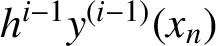 $h^{i-1}y^{(i-1)}(x_{n})$
of Nordsieck vector
 $[y(x)^{T}\hspace {2mm} hy^{\prime }(x)^{T} \ldots h^{r-1}y^{(r-1)}(x)^{T}]^{T}$
. In this paper, we assume that
 ${p=q=s=r-1}$
. Also, the coefficients matrices A and
 $\overline {A}$
are supposed to be strictly lower triangular, and the coefficient matrix V has the form
 $$ \begin{align} V=\left[\begin{array}{@{}ccccc@{}} 1&v_{12}&v_{13}&\cdots&v_{1r}\\[2pt] 0&0&v_{23}&\cdots&v_{2r}\\[2pt] \vdots&\vdots&\vdots&\ddots&\vdots\\[2pt] 0&0&0&\cdots&v_{sr}\\[2pt] 0&0&0&\cdots&0 \end{array}\right]. \end{align} $$
This representation of V ensures that the SGLM in equation (1.2) is zero-stable, as a result of which the matrix V is power bounded. Butcher and Hojjati [Reference Butcher and Hojjati17] proved that an SGLM in Nordsieck form has order p and stage order
 $q=p$
, if and only if
 $$ \begin{align} \exp(cz) = & zA\exp(cz)+z^{2}\overline{A}\exp(cz)+UZ+O(z^{p+1}), \end{align} $$
 $$ \begin{align} \exp(z)Z = & zB\exp(cz)+z^{2}\overline{B}\exp(cz)+VZ+O(z^{p+1}), \end{align} $$
where
 $Z=[1\;\; z\;\; z^{2} \ldots z^{p}]^{T}\in \mathbb {R}^{p+1}$
with z as a complex scalar variable and
 $$ \begin{align*}\exp(cz)=[\exp(c_{1}z)\;\exp(c_{2}z)\;\cdots\; \exp(c_{s}z)]^{T}\in\mathbb{R}^{s}.\end{align*} $$
Let us introduce the matrices
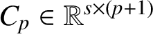 $C_{p}\in \mathbb {R}^{s\times (p+1)}$
,
 ${K_{p}}\in \mathbb {R}^{(p+1)\times (p+1)}$
and
 $E_{p}\in \mathbb {R}^{(p+1)\times (p+1)}$
as follows:
 $$ \begin{align*}C_{p}=\bigg[\textbf{1}\hspace{2mm} \dfrac{c}{1!}\hspace{2mm} \dfrac{c^{2}}{2!} \cdots \dfrac{c^{p}}{p!}\bigg],\quad {K_{p}}:=[{\textbf{0}}\hspace{2mm} e_{1}\hspace{2mm} e_{2} \cdots e_{p}],\end{align*} $$
 $$ \begin{align*}E_{p}=\exp({K_{p}})=\left[\begin{array}{@{}c@{\hspace{2mm}}c@{\hspace{2mm}}c@{\hspace{2mm}}c@{\hspace{2mm}}c@{}} 1 & \dfrac{1}{1!} & \dfrac{1}{2!} & \cdots & \dfrac{1}{p!} \\[8pt] 0 &1 & \dfrac{1}{1!} & \cdots & \dfrac{1}{(p-1)!}\\[8pt] 0 & 0 & 1& \ddots& \vdots \\[8pt] \vdots&\vdots&\vdots&\ddots&\dfrac{1}{1!}\\[8pt] 0&0&0&\cdots&1 \end{array}\right],\end{align*} $$
with
 $c^{j}=[c_{1}^{j} c_{2}^{j} \cdots c_{s}^{j}]^{T}\in \mathbb {R}^{s}$
and
 $e_{j}$
as the jth unit vector in
 $\mathbb {R}^{p+1}$
. Considering these matrices, results in equivalent conditions for the order and stage order conditions from equations (1.4) and (1.5) are given by
 $$ \begin{align} U = C_{p}-A\,C_{p}\,K_{p}-\overline{A}\,C_{p}\,K_{p}^{2}, \end{align} $$
 $$ \begin{align} V = E_{p}-B\,C_{p}\,K_{p}-\overline{B}\,C_{p}\,K_{p}^{2}, \end{align} $$
respectively. Partitioning the matrices
 $C_{p}\,K_{p}$
and
 $C_{p}\,K_{p}^{2}$
as
 $$ \begin{align*}\begin{array}{@{}c@{}} C_{p}\,K_{p}=\bigg[\textbf{0}\hspace{2pt}\bigg|\hspace{2pt}\textbf{1}\hspace{2mm}c \cdots \dfrac{c^{p-1}}{(p-1)!}\bigg]=[\textbf{0}\hspace{2pt}|\hspace{2pt}C_{p-1}],\\[12pt] C_{p}\,K_{p}^{2}=\bigg[\textbf{0}\hspace{2pt}\bigg|\hspace{2pt}\textbf{0}\hspace{2mm}\textbf{1}\hspace{2mm}c \cdots \dfrac{c^{p-2}}{(p-2)!}\bigg]=[\textbf{0}\hspace{2pt}|\hspace{2pt}\widetilde{C}],\\[12pt] E_{p}=[e_{1}\hspace{2pt}|\hspace{2pt}\widetilde{E}],\quad V=[e_{1}\hspace{2pt}|\hspace{2pt}\widetilde{V}], \end{array}\end{align*} $$
relation (1.7) leads to an expression for the matrix B in terms of V,
 $\overline {B}$
and c as
 $$ \begin{align} B=(\widetilde{E}-\widetilde{V}-\overline{B}\,\widetilde{C})\,C_{p-1}^{-1}. \end{align} $$
The stability properties of SGLMs in equation (1.2) are characterized using the basic test equation
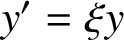 $y^{\prime }=\xi y$
[Reference Dahlquist26], where
 $\xi \in \mathbb {C}$
. Applying such methods to this test equation leads to the recurrence equation
 $y^{[n]}=M(z)y^{[n-1]}$
,
 $n\geq 1$
, with
 $z=h\xi $
, where the stability matrix
 $M(z)$
is given by
 $$ \begin{align*}M(z)=V+(zB+z^{2}\overline{B})(I-zA-z^{2}\overline{A})^{-1}U,\end{align*} $$
and the characteristic polynomial of
 $M(z)$
, as the stability function, is defined by
 $$ \begin{align*}p(w,z)=\det(wI-M(z)).\end{align*} $$
Definition 1. The method in equation (1.2) is said to possess a Runge–Kutta stability (RKS) property if its stability function has the special form
 $$ \begin{align*} p(w,z) = w^{r-1} (w - R(z)), \end{align*} $$
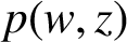
and a quadratic stability (QS) property if
 $p(w,z)$
has only two nonzero roots, that is, it is in the form
 $$ \begin{align*} p(w,z) = w^{r-2} (w^{2}-p_{1}(z)w+p_{0}(z)). \end{align*} $$
Construction of SGLMs with the RKS or QS property and large numbers of r and s requires solving large systems of polynomial equations, which is too complicated a task. To manufacture methods with these properties, one approach is to derive the coefficients of the methods in such a way that an RKS or QS property is guaranteed.
Definition 2. The method in equation (1.2) is said to possess inherent Runge–Kutta stability (IRKS) or inherent quadratic stability (IQS) property if its coefficient matrices satisfy some algebraic constraints which ensure that the method has the RKS or QS property.
Movahedinejad et al. [Reference Movahedinejad, Hojjati and Abdi34] introduced SGLMs in Nordsieck form with IRKS. By relaxing the concept of IRKS to the concept of IQS, methods with such property in the classes of two-step Runge–Kutta (TSRK) methods [Reference Conte, D’Ambrosio and Jackiewicz25], GLMs [Reference Braś and Cardone13, Reference Cardone and Jackiewicz20] and SGLMs [Reference Movahedinejad, Hojjati and Abdi35] have been introduced. SGLMs with IRKS and IQS will be respectively referred to as SIRKS and SIQS. The aim of this paper is to construct explicit SGLMs for the numerical solution of the ODEs in equation (1.1) with a good balance between accuracy and stability properties. So, we search for explicit Nordsieck SGLMs with
 $p=q=s=r-1$
, inherent stability properties and large regions of absolute stability together with reasonably small error constants.
The rest of this paper is organized along the following lines. In Section 2, we discuss SGLMs with IRKS and IQS properties, and then give an approach to construct explicit Nordsieck SIRKS and SIQS with a large area of the stability region. Some examples of such methods are given in Section 3, and their stability regions are compared with those of GLMs with IQS investigated in [Reference Braś and Cardone13] and of Runge–Kutta methods of the same order. To show the accuracy and efficiency of the constructed methods and verify the theoretical results, we present some numerical experiments in Section 4. Finally, the work in the paper is summarized in Section 5.
2 SIRKS and SIQS with large region of absolute stability
The stability function of SGLMs in equation (1.2) takes the form
 $$ \begin{align*} p(w,z) = w^{r}-p_{r-1}(z)w^{r-1}+\cdots+(-1)^{r}p_{0}(z), \end{align*} $$
where
 $p_{j}(z)$
,
 $j=0,1,\ldots ,r-1$
, are polynomials of degree
 $2s$
, depending on the parameters of the methods. Construction of the methods with RKS or QS requires solving the system of nonlinear equations
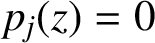 $p_{j}(z)=0$
for
 $j=0,1,\ldots ,r-2$
or
 $j=0,1,\ldots ,r-3$
, respectively. However, the task is too complicated for the methods with large numbers of s and r. Nevertheless, some interrelationships among the coefficients matrices of the method have been obtained which are sufficient conditions to possess RKS [Reference Movahedinejad, Hojjati and Abdi34] or QS [Reference Movahedinejad, Hojjati and Abdi35]. These interrelationships are respectively referred to as IRKS or IQS conditions.
The sufficient conditions for Nordsieck SIRKS with
 $p=q=s=r-1$
are [Reference Movahedinejad, Hojjati and Abdi34]
 $$ \begin{align} B\overline{A}\equiv X\overline{B},\quad BA+\overline{B}\equiv XB,\quad BU\equiv XV-VX \end{align} $$
for some matrix X, and
 $$ \begin{align} \det(wI-V)=w^{p}(w-1). \end{align} $$
Here, the relation
 $\Delta \equiv \Gamma $
means that the matrices
 $\Delta $
and
 $\Gamma $
are identical except possibly in their first rows. The matrix X appearing in equation (2.1) takes the form
 $$ \begin{align*} X=\left[\begin{array}{@{}cccc|c@{}} x_{1,1} & x_{1,2} & \cdots & x_{1,r-1} & x_{1,r} \\ \hline 1 & 0 & \cdots & 0 & x_{2,r} \\ 0 & 1 & \cdots & 0 & x_{3,r} \\ \vdots & \vdots & \ddots & \vdots & \vdots \\ 0 & 0 & \cdots & 1 & x_{r,r} \end{array}\right]. \end{align*} $$
Although in [Reference Movahedinejad, Hojjati and Abdi34] the conditions for SIRKS have been obtained for
 $x_{1j}=x_{ir}=0$
,
 $i,j=1,2,\ldots ,r$
, it is easy to show that equation (2.1) together with equation (2.2) are sufficient conditions for arbitrary values of
 $x_{1j}$
and
 $x_{ir}$
.
The IQS conditions for the Nordsieck methods with upper triangular form in equation (1.3) for the matrix V and
 $p=q=s=r-1$
are
 $$ \begin{align} B\overline{A}\;\dot\equiv\, X\overline{B},\quad BA+\overline{B}\;\dot\equiv\, XB,\quad BU\,\dot\equiv\, XV-VX, \end{align} $$
in which the structure of the matrix X is given by
 $$ \begin{align*} X=\left[\begin{array}{@{}ccccc|c@{}} x_{1,1} & x_{1,2} & x_{1,3} & \cdots & x_{1,r-1} & x_{1,r} \\ x_{2,1} & x_{2,2} & x_{2,3} & \cdots & x_{2,r-1} & x_{2,r} \\ \hline 0 & 1 & 0 & \cdots & 0 & x_{3,r} \\ 0 & 0 & 1 & \cdots & 0 & x_{4,r} \\ \vdots & \vdots & \vdots & \ddots & \vdots & \vdots \\ 0 & 0 & 0 & \cdots & 1 & x_{r,r} \end{array}\right], \end{align*} $$
and the relation
 $\Delta \,\dot \equiv \,\Gamma $
means that the matrices
 $\Delta $
and
 $\Gamma $
are identical except possibly in their first two rows.
To search for SGLMs with a large region of absolute stability, two main steps should be followed. The first step is to impose the order conditions and IRKS or IQS conditions. The second is to use the free remaining parameter(s) to search for methods with a large region of absolute stability. To do this, we consider SGLMs in equation (1.2) with
 $p=q=s=r-1$
and choose the abscissa vector c in advance. By equations (1.6) and (1.8), we derive the matrices U and B in terms of A,
 $\overline {A}$
,
 $\overline {B}$
, V and abscissa vector c. Then, we solve the system of equations corresponding to IRKS or IQS conditions with respect to elements of matrices A,
 $\overline {A}$
,
 $\overline {B}$
, V and X. This leads to a family of SGLMs with IRKS or IQS depending on the vector
 $\mathbf {m}$
of the remaining free parameters. For the second step of the search, we find the elements of the vector
 $\mathbf {m}$
by solving the minimization problem
 $$ \begin{align} \min\;(-\text{area}(\mathbf{m})), \end{align} $$
in which the objective function
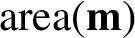 $\text {area}(\mathbf {m})$
is the area of the intersection of the region of absolute stability of the method with the negative half plane. This problem is solved using the fminsearch program of Matlab. Here, in a similar way as that explained by Barghi Oskouie et al. [Reference Barghi Oskouie, Hojjati and Abdi11], the function area (
 $\mathbf {m}$
) can be computed by integration in polar coordinates. We refer to [Reference Barghi Oskouie, Hojjati and Abdi11, Reference Conte, D’Ambrosio and Jackiewicz25] for a detailed description of the process of computing this function.
3 Examples of the methods
In this section, we present some examples of the derived SIRKS and SIQS with a large stability region. We also compare the stability regions of the constructed methods with those of GLMs with IQS studied by Braś and Cardone [Reference Braś and Cardone13] and of the Runge–Kutta methods of the same order.
3.1 Methods of order
 $\boldsymbol {p=q=s=r-1=2}$

In this subsection, we search for methods with
 $p=q=s=r-1=2$
in the form
 $$ \begin{align*} \left[ \begin{array}{@{}c|c|c@{}} A & \overline{A} & U \\ \hline &&\\[-4mm] B & \overline{B} & V \\ \end{array} \right]=\left[\begin{array}{@{}cc|cc|ccc@{}} 0 & 0 & 0 & 0 & 1 & u_{12} & u_{13}\\[3pt] a_{21} & 0 & \overline{a}_{21} & 0 & 1 & u_{22} & u_{23}\\ \hline & & & & & & \\[-4mm] b_{11} & b_{12} & \overline{b}_{11} & \overline{b}_{12} 1 & v_{12} & v_{13} \\[3pt] b_{21} & b_{22} & \overline{b}_{21} & \overline{b}_{22} & 0 & 0 & v_{23} \\[3pt] b_{31} & b_{32} & \overline{b}_{31} & \overline{b}_{32} & 0 & 0 & 0 \\ \end{array}\right]. \end{align*} $$
3.1.1 Methods with IRKS property
First, we search for the methods with IRKS property. Considering the abscissa vector
 $c=[0\hspace {2mm}1]^{T}$
, computing U and B respectively by equations (1.6) and (1.8), and solving the IRKS conditions in equation (2.1) lead to a 3-parameter family of the methods depending on the vector
 $\mathbf {m}=[\overline {a}_{21},\overline {b}_{31},\overline {b}_{32}]$
. Now, we search for the methods with a large stability region by solving the minimization problem in equation (2.4) for these free parameters to get their optimum values. This approach gives the coefficient matrices of the SIRKS of order two as
 $$ \begin{align*} \begin{array}{l} A=\left[\begin{array}{@{}c@{\hspace{2mm}}c@{}} 0 &0\\ 1 & 0 \end{array}\right],\quad \overline{A}=\left[\begin{array}{@{}c@{\hspace{2mm}}c@{}} 0 &0\\ \frac{76}{291} & 0 \end{array}\right],\quad U=\left[\begin{array}{@{}c@{\hspace{2mm}}c@{\hspace{2mm}}c@{}} 1 & 0 & 0\\[2mm] 1 & 0 & \frac{139}{582} \end{array}\right],\\ \\ B=\left[\begin{array}{@{}c@{\hspace{2mm}}c@{}} \frac{397}{515} & \frac{ 411}{1543}\\[2mm] \frac{6823}{9831} & \frac{3008}{9831}\\[2mm] \frac{858}{5503} & -\frac{858}{5503} \end{array}\right],\quad \overline{B}=\left[\begin{array}{@{}c@{\hspace{2mm}}c@{}} \frac{285}{2459} & \frac{83}{4194}\\[2mm] \frac{778}{1701} & \frac{579}{2114}\\[2mm] \frac{1693}{2270} & \frac{739}{1802} \end{array}\right],\quad V=\left[\begin{array}{@{}c@{\hspace{2mm}}c@{\hspace{2mm}}c@{}} 1 & -\frac{117}{3142} & \frac{305}{3114}\\[2mm] 0 & 0 & -\frac{117}{3142}\\[2mm] 0 & 0 & 0 \end{array}\right]. \end{array} \end{align*} $$
The area of the stability region of the method is approximately equal to 38.22.
3.1.2 Methods with IQS property
To find methods with larger regions of absolute stability, we turn our attention to construct methods with the IQS property instead of IRKS property. Again, we first consider the abscissa vector
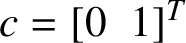 $c=[0\hspace {2mm}1]^{T}$
and compute the matrices U and B respectively by equations (1.6) and (1.8), and solve the IQS conditions in equation (2.3). This lead to a 7-parameter family of the methods depending on the vector
 $$ \begin{align*} \mathbf{m}=[\overline{a}_{21},\overline{b}_{11},\overline{b}_{12},\overline{b}_{31},\overline{b}_{32},v_{12},v_{13}]. \end{align*} $$
Solving the minimization problem in equation (2.4) in terms of these free parameters leads to SIQS of order two with the coefficients matrices
 $$ \begin{align*} \begin{array}{l} A=\left[\begin{array}{@{}c@{\hspace{2mm}}c@{}} 0 &0\\ 1 & 0 \end{array}\right],\quad \overline{A}=\left[\begin{array}{@{}c@{\hspace{2mm}}c@{}} 0 &0\\ \frac{157}{2298} & 0 \end{array}\right],\quad U=\left[\begin{array}{@{}c@{\hspace{2mm}}c@{\hspace{2mm}}c@{}} 1 & 0 & 0\\[2mm] 1 & 0 & \frac{496}{1149} \end{array}\right], \\[18pt] B=\left[\begin{array}{@{}c@{\hspace{2mm}}c@{}} \frac{296}{545} & \frac{361}{1772}\\[2mm] \frac{997}{2144} & \frac{1147}{2144}\\[2mm] -\frac{788}{1065} & \frac{788}{1065} \end{array}\right],\quad \overline{B}=\left[\begin{array}{@{}c@{\hspace{2mm}}c@{}} \frac{230}{5321} & \frac{125}{2528}\\[2mm] \frac{157}{3209} & \frac{339}{3506}\\[2mm] -\frac{185}{41594} & \frac{332}{1255} \end{array}\right],\quad V=\left[\begin{array}{@{}c@{\hspace{2mm}}c@{\hspace{2mm}}c@{}} 1 & \frac{381}{1505} & \frac{531}{2608}\\[2mm] 0 & 0 & \frac{1689}{5288} \\[2mm] 0 & 0 & 0 \end{array}\right]. \end{array} \end{align*} $$
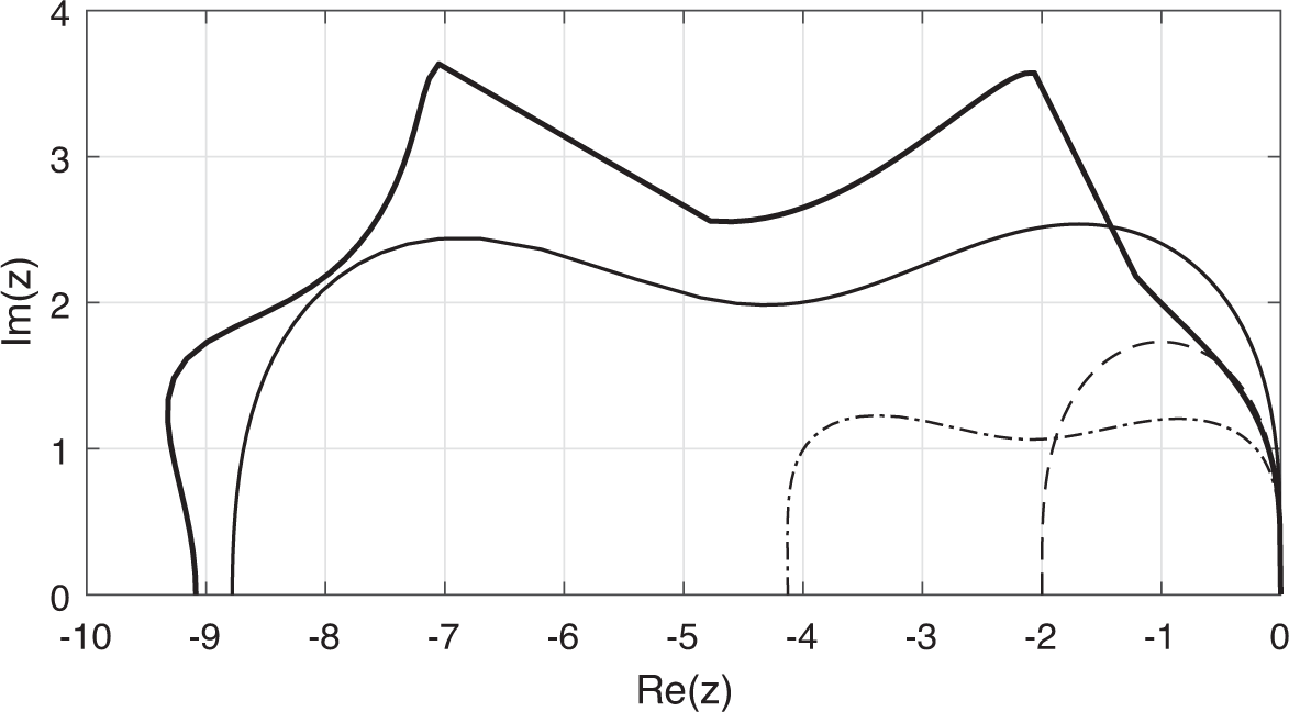
The area of the stability region of this method is approximately equal to 48.56 which is significantly larger than that for the above-mentioned SIRKS in this subsection.
The stability regions of the constructed methods in this subsection, together with those of GLMs with IQS constructed in [Reference Braś and Cardone13] and of the Runge–Kutta method of the same order, are plotted in Figure 1.
Stability regions of SIRKS (thin solid line) and SIQS (thick solid line) of order
 $p=q=s=r-1=2$
together with those for GLM with IQS of order
 $p=q=s=r-1=2$
(dash–dotted line) and the Runge–Kutta method (dashed line) of order
 $p=s=2$
.

3.2 Methods of order
$\boldsymbol {p=q=s=r-1=3}$

In this subsection, we search for methods with
 $p=q=s=r-1=3$
and a large region of absolute stability in the form
 $$ \begin{align*} \left[ \begin{array}{@{}c|c|c@{}} A & \overline{A} & U \\ \hline &&\\[-4mm] B & \overline{B} & V \\ \end{array} \right]=\left[\renewcommand\arraystretch{1.5}\begin{array}{@{}ccc|ccc|cccc@{}} 0 & 0 & 0 & 0 & 0 & 0 & 1 & u_{12} & u_{13} & u_{14}\\ a_{21} & 0 & 0 & \overline{a}_{21} & 0 & 0 & 1 & u_{22} & u_{23} & u_{24}\\ a_{31} & a_{32} & 0 & \overline{a}_{31} & \overline{a}_{32} & 0 & 1 & u_{32} & u_{33} & u_{34}\\[4pt] \hline & & & & & & \\[-5mm] b_{11} & b_{12} & b_{13} & \overline{b}_{11} & \overline{b}_{12} & \overline{b}_{13} &1 & v_{12} & v_{13} & v_{14}\\ b_{21} & b_{22} & b_{23} & \overline{b}_{21} & \overline{b}_{22} & \overline{b}_{23} &0 & 0 & v_{23} & v_{24}\\ b_{31} & b_{32} & b_{33} & \overline{b}_{31} & \overline{b}_{32} & \overline{b}_{33} &0 & 0 & 0 & v_{34}\\ b_{41} & b_{42} & b_{43} & \overline{b}_{41} & \overline{b}_{42} & \overline{b}_{43} &0 & 0 & 0 & 0 \end{array}\right]. \end{align*} $$
3.2.1 Methods with IRKS property
As in the previous subsection, we first search for explicit Nordsieck methods with IRKS. For the abscissa vector
 $c=[0\;\; 1/2\; \;1]^{T}$
, after satisfying the order, stage order and IRKS conditions, we obtain a 5-parameter family of the methods depending on the vector
 $\mathbf {m}=[a_{31},a_{32},\overline {a}_{31},\overline {a}_{32},\overline {b}_{42}]$
. Solving the minimization problem in equation (2.4) for these free parameters leads to SIRKS of order three with the coefficients matrices
 $$ \begin{align*} \begin{array}{l} A=\left[\begin{array}{@{}c@{\hspace{2mm}}c@{\hspace{2mm}}c@{}} 0 & 0 & 0\\[2mm] \frac{1552}{1947} & 0 & 0\\[2mm] -\frac{1807}{1549} & -\frac{4408}{1265} & 0 \end{array}\right],\quad \overline{A}=\left[\begin{array}{@{}c@{\hspace{2mm}}c@{\hspace{2mm}}c@{}} 0 & 0 & 0\\[2mm] \frac{250}{3799} & 0 & 0\\[2mm] \frac{542}{363} & \frac{41237}{21993} & 0 \end{array}\right],\quad U=\left[\begin{array}{@{}c@{\hspace{2mm}}c@{\hspace{2mm}}c@{\hspace{2mm}}c@{}} 1 & 0 & 0 & 0\\[2mm] 1 & -\frac{971}{3268} & \frac{292}{4933} & \frac{1}{48}\\[2mm] 1 & \frac{6917}{1224} & -\frac{3069}{2726} & -\frac{637}{1900} \end{array}\right], \\ \\ B=\left[\begin{array}{@{}c@{\hspace{2mm}}c@{\hspace{2mm}}c@{}} \frac{230}{433} & \frac{725}{1287} & \frac{54}{4189}\\[2mm] -\frac{2787}{4201} & \frac{1607}{1004} & \frac{584}{9297}\\[2mm] -\frac{1301}{383} & \frac{1804}{559} & \frac{216}{1273}\\[2mm] -\frac{9941}{2294} & \frac{8057}{1957} & \frac{1186}{5479} \end{array}\right],\quad \overline{B}=\left[\begin{array}{@{}c@{\hspace{2mm}}c@{\hspace{2mm}}c@{}} \frac{29}{1549} & \frac{458}{2815} & 0\\[2mm] -\frac{353}{854} & \frac{4169}{7763} & 0\\[2mm] -\frac{981}{551} & \frac{347}{348} & 0\\[2mm] -\frac{1139}{376} & \frac{1673}{2218} & 0 \end{array}\right],\quad V=\left[\begin{array}{@{}c@{\hspace{2mm}}c@{\hspace{2mm}}c@{\hspace{2mm}}c@{}} 1 & -\frac{809}{7533} & \frac{109}{4537} & \frac{34}{4021}\\[2mm] 0 & 0 & \frac{101}{7652} & 0\\[2mm] 0 & 0 & 0 & \frac{101}{7652}\\[2mm] 0 & 0 & 0 & 0 \end{array}\right]. \end{array} \end{align*} $$
The area of the stability region of this method is approximately equal to 36.78.
3.2.2 Methods with IQS property
In the same manner to find methods with IQS and the abscissa vector
 $c=[0\; \; 1/2\; \;1]^{T}$
, we obtain a 12-parameter family of the methods depending on the vector
 $$ \begin{align*} \mathbf{m}=[a_{32},\overline{a}_{31},\overline{a}_{32},\overline{b}_{11},\overline{b}_{12},\overline{b}_{13}, \overline{b}_{41},\overline{b}_{42},\overline{b}_{43},v_{12},v_{13},v_{14}]. \end{align*} $$
Solving the minimization problem in equation (2.4) for these free parameters leads to SIQS of order three with the coefficient matrices
 $$ \begin{align*} \begin{array}{l} A=\left[\begin{array}{@{}c@{\hspace{2mm}}c@{\hspace{2mm}}c@{}} 0 & 0 & 0\\[2mm] \frac{1}{2} & 0 & 0\\[2mm] \frac{2656}{3199} & \frac{543}{3199} & 0 \end{array}\right],\quad \overline{A}=\left[\begin{array}{@{}c@{\hspace{2mm}}c@{\hspace{2mm}}c@{}} 0 & 0 & 0\\[2mm] \frac{383}{4715} & 0 & 0\\[2mm] \frac{250}{28671} & \frac{67}{6640} & 0 \end{array}\right],\quad U=\left[\begin{array}{@{}c@{\hspace{2mm}}c@{\hspace{2mm}}c@{\hspace{2mm}}c@{}} 1 & 0 & 0 & 0\\[2mm] 1 & 0 & \frac{124}{2833} & \frac{1}{48}\\[2mm] 1 & 0 & \frac{560}{1413} & \frac{139}{990} \end{array}\right], \end{array} \end{align*} $$
 $$ \begin{align*} \begin{array}{l} B=\left[\begin{array}{@{}c@{\hspace{2mm}}c@{\hspace{2mm}}c@{}} \frac{1679}{717} & -\frac{1698}{899} & \frac{336}{2477}\\[2mm] \frac{545}{594} & -\frac{737}{2527} & \frac{327}{874}\\[2mm] -\frac{786}{2569} & -\frac{445}{316} & \frac{2369}{1382}\\[2mm] \frac{1436}{127} & -\frac{2682}{211} & \frac{2437}{1736} \end{array}\right],\quad \overline{B}=\left[\begin{array}{@{}c@{\hspace{2mm}}c@{\hspace{2mm}}c@{}} \frac{1175}{2372} & \frac{300}{2179} & \frac{559}{2615}\\[2mm] \frac{60}{989} & \frac{343}{4689} & \frac{483}{5498}\\[2mm] -\frac{1493}{3014} & \frac{420}{2129} & \frac{896}{3111}\\[2mm] \frac{6135}{2351} & \frac{1492}{1639} & \frac{2467}{1723} \end{array}\right], \quad V=\left[\begin{array}{@{}c@{\hspace{2mm}}c@{\hspace{2mm}}c@{\hspace{2mm}}c@{}} 1 & \frac{346}{841} & \frac{1553}{3362} & \frac{129}{2465}\\[2mm] 0 & 0 & \frac{1776}{3229} & \frac{283}{1258}\\[2mm] 0 & 0 & 0 & -\frac{134}{1979}\\[2mm] 0 & 0 & 0 & 0 \end{array}\right]. \end{array} \end{align*} $$
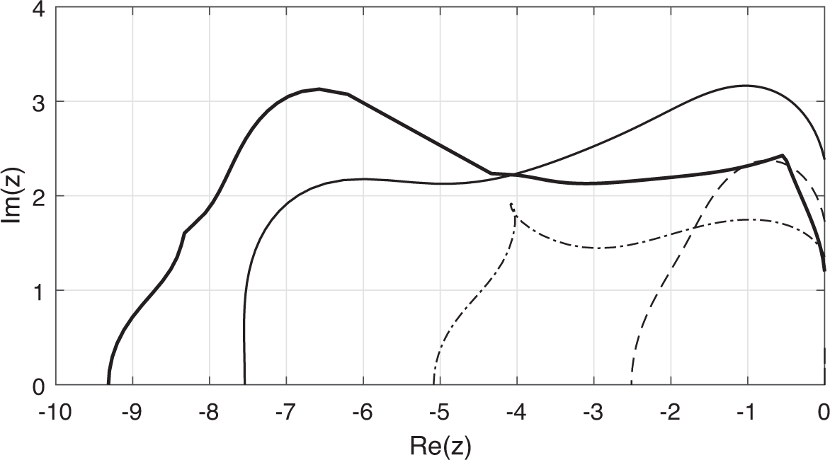
The area of the stability regions of this method is approximately equal to 41.73.
The stability regions of the constructed methods in this subsection together with those of GLMs with IQS constructed in [Reference Braś and Cardone13] and of the Runge–Kutta method of the same order are plotted in Figure 2.
Stability regions of SIRKS (thin solid line) and SIQS (thick solid line) of order
 $p=q=s=r-1=3$
together with those for GLM with IQS of order
 $p=q=s=r-1=3$
(dash–dotted line) and the Runge–Kutta method (dashed line) of order
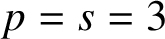 $p=s=3$
.

3.3 Methods of order
$\boldsymbol {p=q=s=r-1=4}$

In this subsection, we search for methods with
 $p=q=s=r-1=4$
and a large region of absolute stability in the form
 $$ \begin{align*} \left[ \begin{array}{@{}c|c|c@{}} A & \overline{A} & U \\ \hline &&\\[-3mm] B & \overline{B} & V \\ \end{array} \right]\hspace{-0.75mm}=\hspace{-0.75mm}\left[\renewcommand\arraystretch{1.5} \begin{array}{@{}cccc|cccc|ccccc@{}} 0 & 0 & 0 & 0 & 0 & 0 & 0 & 0 & 1 & u_{12} & u_{13} & u_{14} & u_{15}\\ a_{21} & 0 & 0 & 0 & \overline{a}_{21} & 0 & 0 & 0 & 1 & u_{22} & u_{23} & u_{24} & u_{25}\\ a_{31} & a_{32} & 0 & 0 &\overline{a}_{31} & \overline{a}_{32} & 0 & 0 & 1 & u_{32} & u_{33} & u_{34} & u_{35}\\ a_{41} & a_{42} & a_{43} & 0 &\overline{a}_{41} & \overline{a}_{42} & \overline{a}_{43} & 0 & 1 & u_{42} & u_{43} & u_{44} & u_{45}\\[4pt] \hline & & & & & & & & & \\[-5mm] b_{11} & b_{12} & b_{13} & b_{14} & \overline{b}_{11} & \overline{b}_{12} & \overline{b}_{13} &\overline{b}_{14} &1 & v_{12} & v_{13} & v_{14} & v_{15}\\ b_{21} & b_{22} & b_{23} & b_{24} & \overline{b}_{21} & \overline{b}_{22} & \overline{b}_{23} &\overline{b}_{24} &0 & 0 & v_{23} & v_{24} & v_{25}\\ b_{31} & b_{32} & b_{33} & b_{34} & \overline{b}_{31} & \overline{b}_{32} & \overline{b}_{33} &\overline{b}_{34} &0 & 0 & 0 & v_{34} & v_{35}\\ b_{41} & b_{42} & b_{43} & b_{44} & \overline{b}_{41} & \overline{b}_{42} & \overline{b}_{43} &\overline{b}_{44} &0 & 0 & 0 & 0 & v_{45}\\ b_{51} & b_{52} & b_{53} & b_{54} & \overline{b}_{51} & \overline{b}_{52} & \overline{b}_{53} &\overline{b}_{54} &0 & 0 & 0 & 0 & 0 \end{array}\right]. \end{align*} $$
3.3.1 Methods with IRKS property
We first search for explicit Nordsieck methods with IRKS and the abscissa vector
 $\mathbf {c}=[1/4\; \;1/2 \; \; 3/4 \; \;1]^{T}$
. By satisfying the order, stage order and IRKS conditions, we obtain a 7-parameter family of the methods depending on the vector
 $\mathbf {m}=[a_{31},a_{32},a_{41},\overline {a}_{31}, \overline {a}_{32},\overline {a}_{41},\overline {a}_{42}]$
. Then, solving the minimization problem in equation (2.4) for these parameters leads to SIRKS of order four with the coefficient matrices
 $$ \begin{align*} \begin{array}{l} A=\left[\begin{array}{@{}c@{\hspace{2mm}}c@{\hspace{2mm}}c@{\hspace{2mm}}c@{}} 0 & 0 & 0 & 0\\[2mm] \frac{2960}{2557} & 0 & 0 & 0\\[2mm] \frac{814}{589} & \frac{453}{647} & 0 & 0\\[2mm] \frac{1435}{1259} & \frac{1136}{649} & 0 & 0 \end{array}\right],\quad \overline{A}=\left[\begin{array}{@{}c@{\hspace{2mm}}c@{\hspace{2mm}}c@{\hspace{2mm}}c@{}} 0 & 0 & 0 & 0\\[2mm] \frac{431}{1903} & 0 & 0 & 0\\[2mm] \frac{396}{995} & \frac{453}{3856} & 0 & 0\\[2mm] \frac{1629}{2854} & \frac{307}{1037} & \frac{9}{69499} & 0 \end{array}\right], \\ \\ U=\left[\begin{array}{@{}c@{\hspace{2mm}}c@{\hspace{2mm}}c@{\hspace{2mm}}c@{\hspace{2mm}}c@{}} 1 & \frac{1}{4} & \frac{1}{32} & \frac{1}{384} & \frac{1}{6144}\\[2mm] 1 & -\frac{1742}{2649} & -\frac{772}{1975} & -\frac{202}{2807} & -\frac{383}{51148}\\[2mm] 1 & -\frac{3020}{2267} & -\frac{596}{641} & -\frac{1671}{7643} & -\frac{286}{8903}\\[2mm] 1 & -\frac{1790}{947} & -\frac{310}{203} & -\frac{385}{1017} & -\frac{181}{3438} \end{array}\right],\quad B=\left[\begin{array}{@{}c@{\hspace{2mm}}c@{\hspace{2mm}}c@{\hspace{2mm}}c@{}} -\frac{1113}{493} & \frac{1815}{193} & -\frac{1892}{161} & \frac{2261}{481}\\[2mm] \frac{109}{26892} & \frac{913}{244} & -\frac{1012}{221} & \frac{11}{6}\\[2mm] 0 & 0 & 0 & 0\\[2mm] -16 & 64 & -80 & 32\\[2mm] 0 & 0 & 0 & 0 \end{array}\right], \\ \\ \overline{B}=\left[\begin{array}{@{}c@{\hspace{2mm}}c@{\hspace{2mm}}c@{\hspace{2mm}}c@{}} \frac{344}{4105} & -\frac{175}{3911} & \frac{148}{2381} & -\frac{107}{4320}\\[2mm] -\frac{2261}{962} & \frac{6045}{643} & -\frac{1892}{161} & \frac{2261}{481}\\[2mm] \frac{109}{26892} & \frac{913}{244} & -\frac{1012}{221} & \frac{11}{6}\\[2mm] 0 & 0 & 0 & 0\\[2mm] -16 & 64 & -80 & 32 \end{array}\right],\quad V=\left[\begin{array}{@{}c@{\hspace{2mm}}c@{\hspace{2mm}}c@{\hspace{2mm}}c@{\hspace{2mm}}c@{}} 1 & \frac{350}{387} & \frac{521}{1306} & -\frac{27}{6896} & -\frac{211}{1960}\\[2mm] 0 & 0 & \frac{673}{923} & \frac{597}{1480} & -\frac{276}{6607}\\[2mm] 0 & 0 & 0 & \frac{673}{923} & \frac{597}{1480} \\[2mm] 0 & 0 & 0 & 0 & 0\\[2mm] 0 & 0 & 0 & 0 & 0 \end{array}\right]. \end{array} \end{align*} $$
The area of the stability region of this method is approximately equal to 31.63.
3.3.2 Methods with IQS property
Now, we are going to construct methods with IQS and the abscissa vector
 $c=[0\; \; 1/3 \;\; 2/3 \; \;1]^{T}$
. By solving the order, stage order and IQS conditions, we obtain a 15-parameter family of the methods depending on the vector
 $$ \begin{align*} \mathbf{m}=[a_{21},a_{31},a_{32},\overline{a}_{31},\overline{a}_{41},\overline{a}_{43}, b_{11},b_{12},b_{13},b_{14},\overline{b}_{11},\overline{b}_{12},\overline{b}_{13}, \overline{b}_{14},x_{35}]. \end{align*} $$
Solving the minimization problem in equation (2.4) for the vector
 $\mathbf {m}$
leads to SIQS of order four with the coefficient matrices
 $$ \begin{align*} \begin{array}{l} A=\left[\begin{array}{@{}c@{\hspace{2mm}}c@{\hspace{2mm}}c@{\hspace{2mm}}c@{}} 0 & 0 & 0 & 0\\[2mm] -\frac{49}{2885} & 0 & 0 & 0\\[2mm] \frac{476}{1647} & \frac{532}{3225} & 0 & 0\\[2mm] \frac{1951}{2579} & \frac{266}{645} & 0 & 0 \end{array}\right],\quad \overline{A}=\left[\begin{array}{@{}c@{\hspace{2mm}}c@{\hspace{2mm}}c@{\hspace{2mm}}c@{}} 0 & 0 & 0 & 0\\[2mm] -\frac{52}{6087} & 0 & 0 & 0\\[2mm] \frac{269}{4447} & \frac{321}{9572} & 0 & 0\\[2mm] \frac{83}{635} & \frac{307}{3220} & \frac{227}{2780} & 0 \end{array}\right],\end{array} \end{align*} $$
 $$ \begin{align*} \begin{array}{l} U=\left[\begin{array}{@{}c@{\hspace{2mm}}c@{\hspace{2mm}}c@{\hspace{2mm}}c@{\hspace{2mm}}c@{}} 1 & 0 & 0 & 0 & 0\\[2mm] 1 & \frac{2977}{8498} & \frac{193}{3011} & \frac{1}{162} & \frac{1}{1944}\\[2mm] 1 & \frac{191}{898} & \frac{138}{1885} & \frac{287}{9883} & \frac{19}{3552}\\[2mm] 1 & -\frac{164}{971} & \frac{481}{8773} & \frac{266}{4623} & \frac{114}{7271}\\[2mm] \end{array}\right],\quad B=\left[\begin{array}{@{}c@{\hspace{2mm}}c@{\hspace{2mm}}c@{\hspace{2mm}}c@{}} \frac{345}{817} & \frac{593}{3723} & \frac{463}{2187} & \frac{215}{1729}\\[2mm] -\frac{835}{524} & \frac{1902}{491} & -\frac{3263}{1048} & \frac{11}{6}\\[2mm] 0 & 0 & 0 & 0\\[2mm] -9 & 36 & -45 & 18\\[2mm] 0 & 0 & 0 & 0 \end{array}\right], \\ \\ \overline{B}=\left[\begin{array}{@{}c@{\hspace{2mm}}c@{\hspace{2mm}}c@{\hspace{2mm}}c@{}} \frac{449}{5131} & -\frac{356}{10305} & \frac{211}{2754} & -\frac{46}{11823}\\[2mm] \frac{391}{3098} & -\frac{782}{1549} & \frac{378}{599} & -\frac{391}{1549}\\[2mm] -\frac{835}{524} & \frac{1902}{491} & -\frac{3263}{1048} & \frac{11}{6}\\[2mm] 0 & 0 & 0 & 0\\[2mm] -9 & 36 & -45 & 18 \end{array}\right],\quad V=\left[\begin{array}{@{}c@{\hspace{2mm}}c@{\hspace{2mm}}c@{\hspace{2mm}}c@{\hspace{2mm}}c@{}} 1 & \frac{443}{5377} & \frac{399}{7159} & \frac{47}{3636} & -\frac{83}{22695}\\[2mm] 0 & 0 & -\frac{237}{4849} & \frac{138}{2299} & \frac{91}{18280}\\[2mm] 0 & 0 & 0 & -\frac{237}{4849} & \frac{138}{2299}\\[2mm] 0 & 0 & 0 & 0 & 0\\[2mm] 0 & 0 & 0 & 0 & 0 \end{array}\right]. \end{array} \end{align*} $$
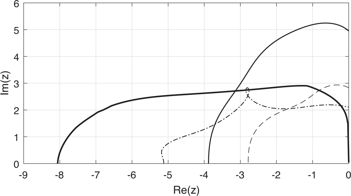
The area of the stability regions of this method is approximately equal to 38.54 which is substantial.
The stability regions of the constructed methods in this subsection together with those of GLMs with IQS constructed in [Reference Braś and Cardone13] and of the Runge–Kutta method of the same order are plotted in Figure 3.
Stability regions of SIRKS (thin solid line) and SIQS (thick solid line) of order
 $p=q=s=r-1=4$
together with those for GLM with IQS of order
 $p=q=s=r-1=4$
(dash–dotted line) and the Runge–Kutta method (dashed line) of order
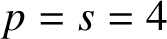 $p=s=4$
.

3.4 Methods of order
$\boldsymbol {p=q=s=r-1=5}$

In this subsection, we search for explicit methods with
 $p=q=s=r-1=5$
and a large region of absolute stability. After an extensive search for methods with IRKS, we were not able to find such methods. However, we could find a
 $23$
-parameter family of the methods of order
 $p=5$
with the abscissa vector
 $\mathbf {c}=[0\; \;1/4\;\;2/4 3/4\;\;1]^{T}$
and IQS property. These free parameters are included in the vector
 $\mathbf {{m}}$
as
 $$ \begin{align*} \textbf{m}=[a_{31},a_{32},a_{41},a_{51},a_{52}, \overline{a}_{21},\overline{a}_{31}, \overline{a}_{32},\overline{a}_{41},\overline{a}_{42},\overline{a}_{43}, \overline{a}_{53},\overline{a}_{54},b_{1i},\overline{b}_{1i}],\quad i=1,2,\ldots,5. \end{align*} $$
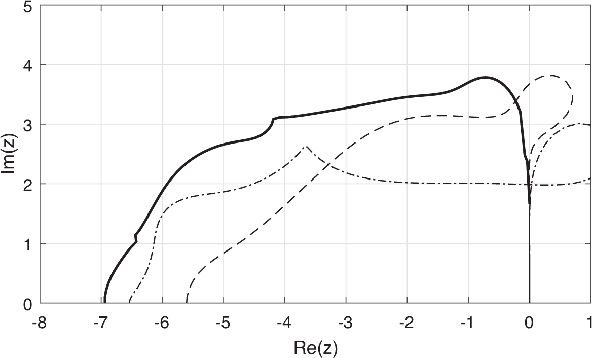
Stability region of SIQS (thick solid line) of order
 $p=q=s=r-1=5$
together with that for GLM with IQS of order
 $p=q=s=r-1=5$
(dash–dotted line) and the Runge–Kutta method (dashed line) of order
 $p=s-1=5$
reported in [Reference Butcher15].

Now, solving the minimization problem in equation (2.4) leads to SIQS of order five with the coefficient matrices
 $$ \begin{align*} \begin{array}{l} A=\left[\begin{array}{@{}c@{\hspace{2mm}}c@{\hspace{2mm}}c@{\hspace{2mm}}c@{\hspace{2mm}}c@{}} 0 & 0 & 0 & 0 & 0\\[2mm] \frac{1189}{3735} & 0 & 0 & 0 & 0\\[2mm] \frac{989}{2830} & \frac{456}{1727} & 0 & 0 & 0\\[2mm] \frac{243}{1126} & \frac{1727}{4998} & \frac{1357}{4191} & 0 & 0\\[2mm] -\frac{69}{7505} & -\frac{66}{2813} & \frac{2083}{1787} & 0 & 0 \end{array}\right],\quad \overline{A}=\left[\begin{array}{@{}c@{\hspace{2mm}}c@{\hspace{2mm}}c@{\hspace{2mm}}c@{\hspace{2mm}}c@{}} 0 & 0 & 0 & 0 & 0\\[2mm] \frac{288}{2939 } & 0 & 0 & 0 & 0\\[2mm] \frac{265}{2418 } & \frac{255}{6701} & 0 & 0 & 0\\[2mm] \frac{99}{1598} & \frac{847}{11069} & \frac{96}{2257}& 0 & 0\\[2mm] -\frac{344}{7533} & \frac{ 246}{1477} & \frac{75}{2366} & \frac{235}{3632} & 0 \end{array}\right], \\ \\ U=\left[\begin{array}{@{}c@{\hspace{2mm}}c@{\hspace{2mm}}c@{\hspace{2mm}}c@{\hspace{2mm}}c@{\hspace{2mm}}c@{}} 1 & 0 & 0 & 0 & 0 & 0\\[2mm] 1 & \frac{-373}{5458 } & \frac{-176}{2637} & \frac{1}{384 } & \frac{1}{6144} & \frac{1}{122880}\\[2mm] 1 & \frac{-331}{2916 } & \frac{-240}{2707} & \frac{226}{73651} & \frac{49}{67366} & \frac{13}{109851}\\[2mm] 1 & \frac{-8238}{60961 } & \frac{-1074}{7255} & \frac{-188}{8803 } & \frac{-34}{15669} & \frac{-1}{136912}\\[2mm] 1 & \frac{-127}{955 } & \frac{-547}{1859 } & \frac{-178}{2111 } & \frac{-34}{3427} & \frac{-9}{26323} \end{array}\right],\quad B=\left[\begin{array}{@{}c@{\hspace{2mm}}c@{\hspace{2mm}}c@{\hspace{2mm}}c@{\hspace{2mm}}c@{}} \frac{392}{1347} & \frac{ 519}{1621} &\frac{2212}{4825} & \frac{275}{7688 } & \frac{457}{3122}\\[2mm] \frac{-539}{248} & \frac{2143}{441} & \frac{-6410}{839} & \frac{4493}{545 } & \frac{-2132}{931}\\[2mm] \frac{1151}{148} & \frac{-3869}{104 } & \frac{6651}{103} & \frac{-2843}{54 } & \frac{55073}{3147}\\[2mm] 0 & 0 & 0 & 0 & 0\\[2mm] 96 & -448 & 768 & -576 & 160\\[2mm] 0 & 0 & 0 & 0 & 0 \end{array}\right], \end{array} \end{align*} $$
 $$ \begin{align*} \begin{array}{l} \overline{B}=\left[\begin{array}{@{}c@{\hspace{2mm}}c@{\hspace{2mm}}c@{\hspace{2mm}}c@{\hspace{2mm}}c@{}} \frac{224}{2719} & \frac{2128}{21181} & \frac{-14}{33325}& \frac{2170}{27487} & \frac{-219}{7037}\\[2mm] \frac{-831}{1252} & \frac{487}{324} & \frac{-1179}{602} & \frac{919}{687} & \frac{-55}{964}\\[2mm] \frac{-518}{377} & \frac{2879}{449 } & \frac{-5529}{503} & \frac{4493}{545 } & \frac{-2132}{931}\\[2mm] \frac{1151}{148} & \frac{-3869}{104} & \frac{6651}{103} & \frac{-2843}{54 } & \frac{55073}{3147}\\[2mm] 0 & 0 & 0 & 0 & 0\\[2mm] 96 & -448 & 768 & -576 & 160 \end{array}\right],\quad V=\left[\begin{array}{@{}c@{\hspace{2mm}}c@{\hspace{2mm}}c@{\hspace{2mm}}c@{\hspace{2mm}}c@{\hspace{2mm}}c@{}} 1 & \frac{-1022}{4059 } & \frac{-625}{2938 } & \frac{-205}{5557} & \frac{-23}{4291} & \frac{-9}{89692}\\[2mm] 0 & 0 & \frac{-2241}{4987} & \frac{-654}{3067 } & \frac{-293}{8450} & \frac{-17}{107530}\\[2mm] 0 & 0 & 0 & \frac{323}{2180 }& \frac{143}{3892 } & \frac{-75}{4628}\\[2mm] 0 & 0 & 0 & 0 & \frac{323}{2180} & \frac{143}{3892}\\[2mm] 0 & 0 & 0 & 0 & 0 & 0\\[2mm] 0 & 0 & 0 & 0 & 0 & 0 \end{array}\right]. \end{array} \end{align*} $$
The area of the stability regions of this method is approximately equal to 39.54.
The stability region of the constructed method in this subsection together with that of GLMs with IQS constructed in [Reference Braś and Cardone13] and of the Runge–Kutta method of the same order are plotted in Figure 4.
4 Numerical experiments
In this section, the results of some numerical experiments are provided to show the accuracy and efficiency together with the theoretical results of the constructed methods.
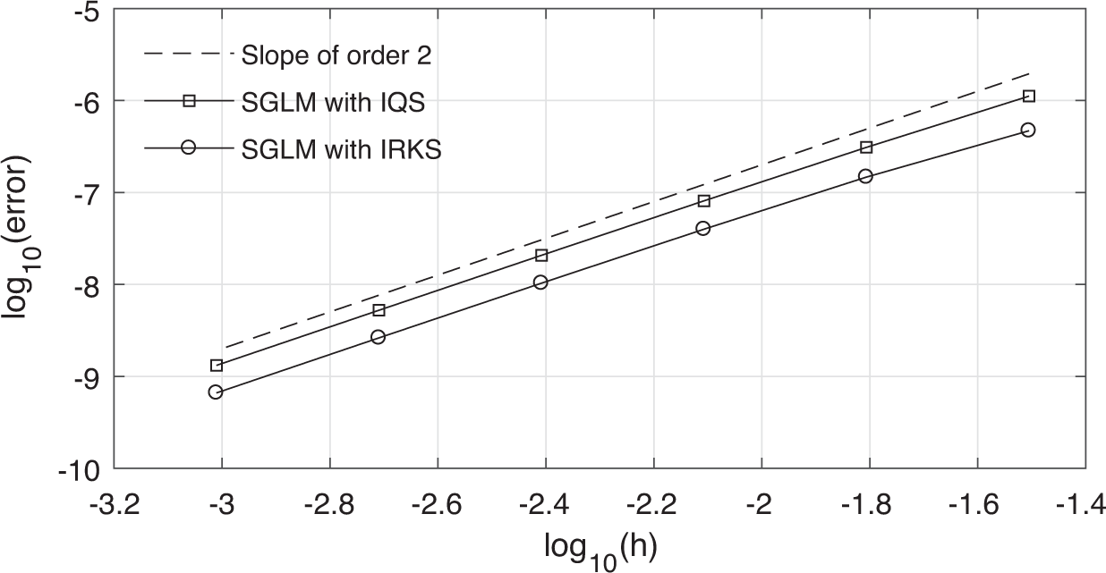
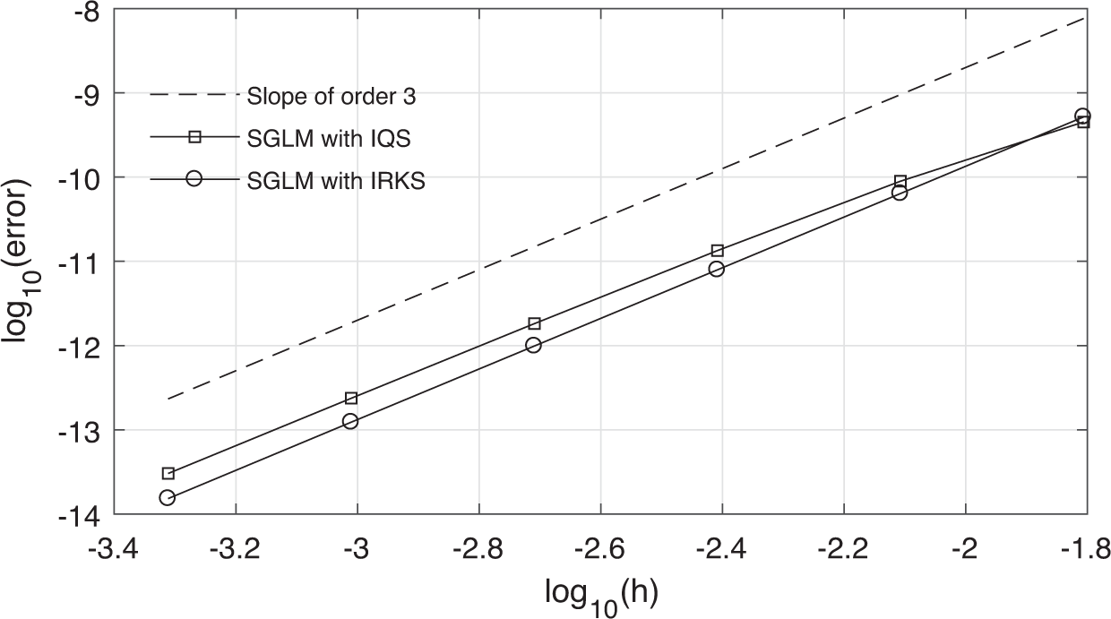
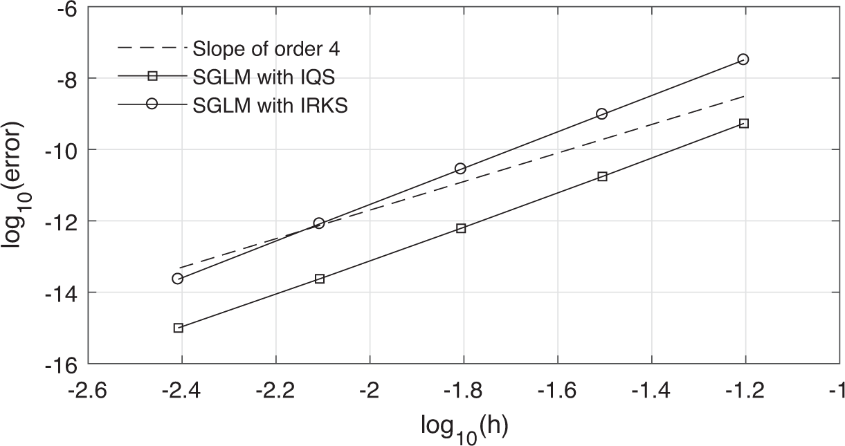
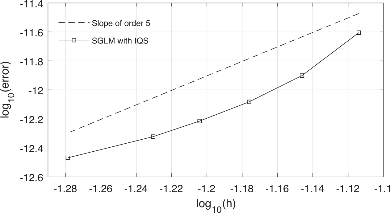
To confirm the order of convergence of the constructed methods with IQS and IRKS, we consider the Prothero–Robinson problem [Reference Prothero and Robinson36]:
 $$ \begin{align*} y^{\prime}=-16y+15e^{-x},\quad y(0)=2, \end{align*} $$
with the exact solution
 $y(x)=e^{-x}+e^{-16x}$
. We have applied the methods to this problem for various fixed stepsizes
 $h=1/2^{k}$
for several integer values of k. The norm of the global error versus the stepsize for the methods of order
 $p=2,3,4$
and
 $5$
at the endpoint of the interval integration
 $\overline {x}=2$
are plotted in Figures 5–8 in double logarithmic scale. These results confirm the high accuracy of the constructed methods and illustrate that the errors of the methods decrease with the expected orders.
Order verification for the SGLMs of order two.

Order verification for the SGLMs of order three.

Order verification for the SGLMs of order four.

Order verification for the SGLM of order five.

To show the superiority of the wider absolute stability region, we compare the global errors of the constructed SIQS of order
 $p=q=s=r-1=4$
with those of the GLM with IQS of the same order studied in [Reference Braś and Cardone13] for the problem [Reference Abdi and Hojjati8]:
 $$ \begin{align*} \begin{cases} y_{1}^{\prime}=-\alpha y_{1}-\beta y_{2}+(\alpha+\beta-1)e^{-x},& y_{1}(0)=1,\\[2mm] y_{2}^{\prime}= \beta y_{1}-\alpha y_{2}+(\alpha-\beta-1)e^{-x},& y_{2}(0)=1, \end{cases} \end{align*} $$
with the exact solution
 $y_{1}(x)=y_{2}(x)=e^{-x}$
. The eigenvalues of the Jacobian of this system are
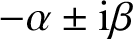 $-\alpha \pm \mathrm {i}\beta $
. We have applied the methods to this problem with the fixed stepsize
 $h=0.1$
,
 $\alpha =50$
and
 $\beta =20$
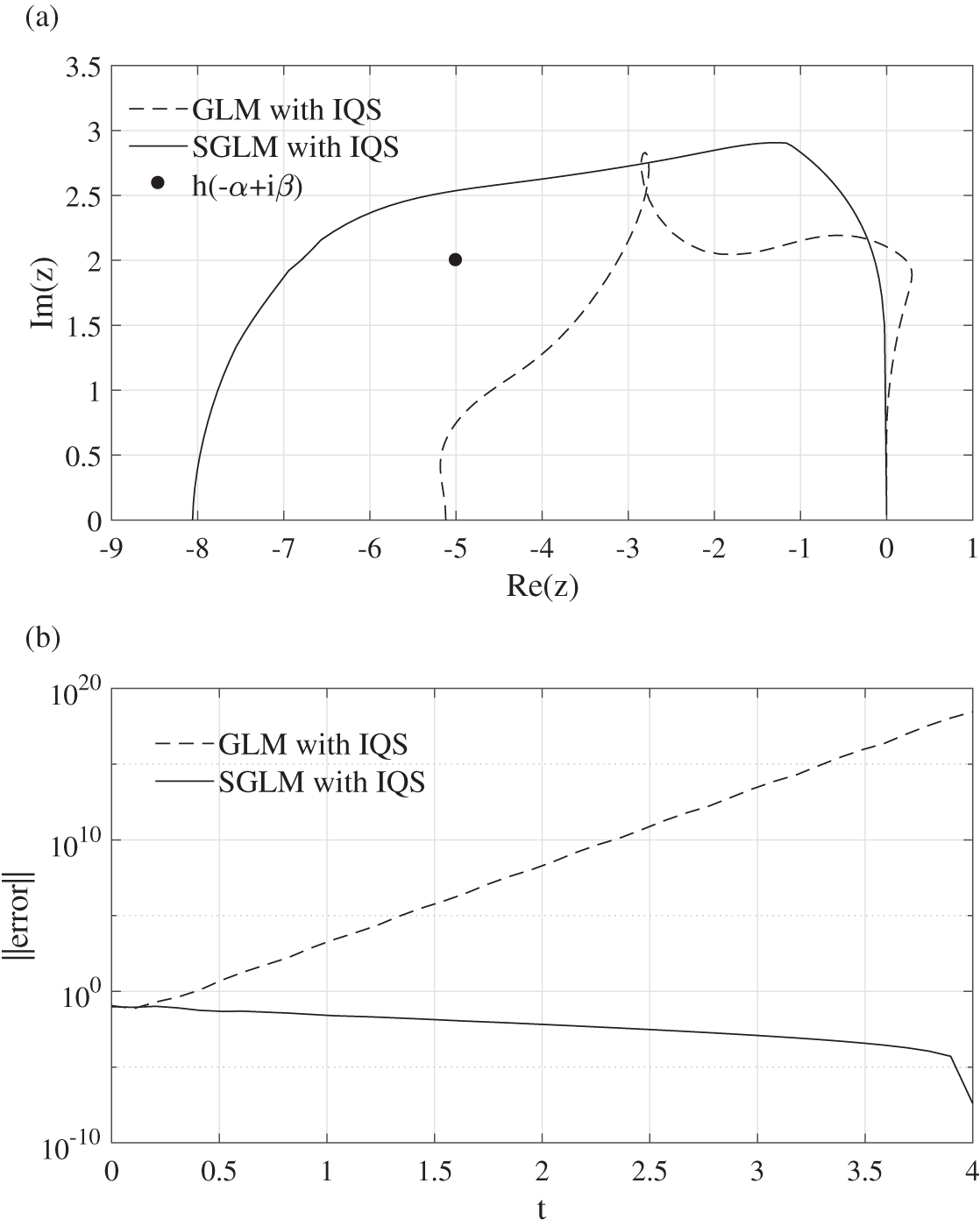
. In Figure 9(a), we have plotted the stability regions of the methods together with the point
 $h(-\alpha +\mathrm {i}\beta )=-5+2\mathrm {i}$
; one can see that this point lies inside the absolute stability region for SGLM while it lies outside that for GLM. As we expect, Figure 9(b) shows that SGLM converges with this stepsize while this is not the case for GLM.
(a) Boundary of the stability regions of SGLM and GLM of order four together with the point
 $h(-\alpha +\mathrm {i}\beta )=-5+2\mathrm {i}$
. (b) Numerical results for these methods with
 $h=0.1$
for the system in equation (4) with
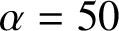 $\alpha =50$
and
 $\beta =20$
.

As our final test, we have applied the SGLMs and GLM with IQS of order four to the nonlinear system [Reference Abdi, Hojjati, Izzo and Jackiewicz9, Reference Constantinescu24, Reference Kulikov33]
 $$ \begin{align} \begin{cases} y_{1}^{\prime}=2xy_{2}^{1/5}y_{4},\\[2mm] y_{2}^{\prime}=10x\exp(5(y_{3}-1))y_{4},\\[2mm] y_{3}^{\prime}=2xy_{4},\\[2mm] y_{4}^{\prime}=-2x\ln (y_{1}), \end{cases} \end{align} $$
with
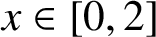 $x\in [0,2]$
and the initial values
 $y(0)=[1\hspace {1.5mm}1\hspace {1.5mm}1\hspace {1.5mm}1]^{T}$
. The exact solution of the problem is given by
 $$ \begin{align*} y(x)=[\exp(\sin(x^{2}))\hspace{2mm} \exp(5\sin(x^{2}))\hspace{2mm} \sin(x^{2})+1\hspace{2mm} \cos(x^{2})]^{T}. \end{align*} $$
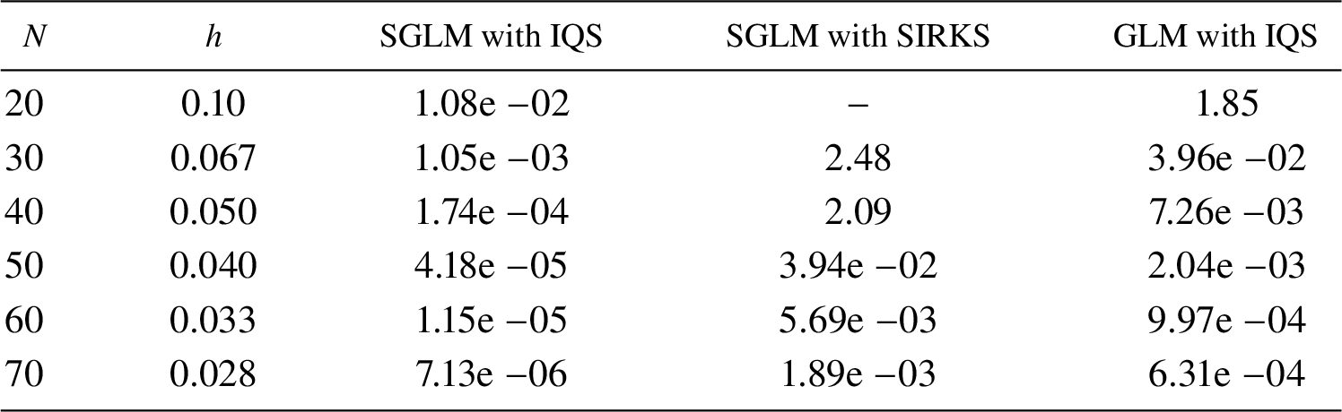
In Table 1, we have listed the global errors of the methods at the endpoint of the interval integration. The results show that the SGLMs which have a wider stability region can integrate this system for a larger range of the stepsizes h. In this table, the symbol “–” is used to show that we cannot proceed to the endpoint of the interval since the methods become divergent.
Global errors for the methods of order four for the problem (4.1).

5 Concluding remarks and future work
In this paper, we described an approach to construct explicit SGLMs of order
 $p=q=s=r-1$
up to five in the Nordsieck form with IRKS and IQS properties. The construction is based on solving an optimization problem with maximum area of the absolute stability region of the method as the objective function. Some examples of such methods were presented in which the constructed SGLMs with IQS have larger absolute stability regions than those for SGLMs with IRKS and GLMs with IQS. As it was shown in the numerical experiments, the constructed SGLMs are more efficient than GLMs of the same order.
Building upon our previous work, future work in this area will address the discussion of various issues related to the development of a solver in a variable-stepsize/variable-order (VSVO) environment based on the proposed methods. Indeed, we plan to develop a code for nonstiff ODEs based on the proposed methods in a VSVO mode and compare its performance with that for the existing ODE solvers such as ode45 from Matlab ODE suite and the codes dim18 and irks14 introduced in [Reference Abdi and Jackiewicz10, Reference Butcher, Chartier and Jackiewicz16].