1. Introduction
Major headwinds associated with the COVID-19 pandemic have had devastating economic consequences around the world, and the scars from these shocks are likely to be sizeable. According to estimates of the IMF World Economic Outlook (WEO) April 2022, cumulative per capita income losses over 2020–2023, compared to pre-pandemic projections, are equivalent to about 2½% of 2019 per capita GDP for the world as whole and over 4% in emerging markets (EM) and developing economies.
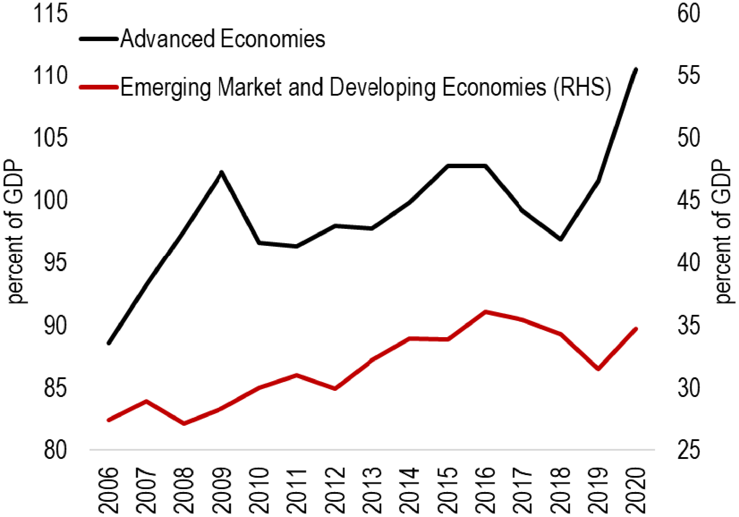
These shocks have occurred in the context of rising corporate debt. Corporate debt as a share of GDP increased significantly in the decade following the global financial crisis (GFC), both in advanced economies (AE) and EM and developing economies. And while there were signs of debt levels moderating after 2016, this trend was reversed in 2020, as debt ratios increased sharply with the pandemic (Figure 1). The fear is that this higher corporate debt may further aggravate the scarring effects associated with the COVID-19 pandemic. The focus of our paper is to shed light on this issue by examining the role of firms’ debt in shaping the response of firms’ investment to (past) recessions.
Nonfinancial corporate debt, loans and debt securities (percent of GDP).
Source: IMF Global Debt Database and authors calculations.
Note: Consistent sample of 70 countries across time: advanced economies (35) and emerging market and developing economies (35). Dotted upper(lower) lines depict the 75th (25th) percentiles of the overall distribution. Solid lines depict the median.

There exists already a well-established literature on the effects of corporate debt on investment and growth. In his seminal paper, Myers (Reference Myers1977) stipulated that highly leveraged firms are unlikely to be able to raise new debt and thus invest in new projects as their profits must be used to pay existing debt holders. His work spawned the literature on debt overhang, highlighting the effect of the level of firm leverage on investment and the negative association between leverage and growth.Footnote 1
The onset of the GFC revived the literature on the effects of high leverage and credit constraints on economic outcomes, especially in AE. One strand of the literature used country-level data to uncover the effects of debt booms in the private sector on overall economic activity: Dell’Ariccia et al. (Reference Dell”Ariccia, Igan, Laeven and Tong2016) find that credit booms often result in financial crises but can also be associated with financial reforms and economic growth. Jordà et al. (Reference Jordà, Schularick and Taylor2013) find that credit-intensive expansions tend to be followed by deeper recessions and slower recoveries.Footnote 2
Another strand of the literature focused on the strength of firms’ balance sheet prior to recessions in determining their overall resilience, relying mostly on firm-level data to show that weak balance sheets could constrain investment. Focusing on the US, Giroud and Mueller (Reference Giroud and Mueller2017) use granular plant-level data to find that firms with more leverage saw bigger declines in employment and investment following the GFC, while Ottonello and Winberry (Reference Ottonello and Winberry2020) find that higher-leverage firms respond less to monetary policy shocks. Using cross-country firm-level data, Duval et al. (Reference Duval, Hong and Timmer2020) find that firms with weaker pre-GFC balance sheets, particularly those exposed to rollover risk, experienced a highly persistent decline in postcrisis total factor productivity growth relative to their less vulnerable counterparts. Kalemli-Ozcan et al. (Reference Kalemli-Ozcan, Laeven and Moreno2022) use European firm-bank matched data and find that firms with higher debt levels pre-GFC reduced their investment more after the crisis, with the effect stronger for firms holding short-term debt in countries with sovereign stress.Footnote 3 Campello et al. (Reference Campello, Graham and Harvey2010) find that credit-constrained firms in the US, Europe, and Asia had to undertake deeper cuts in employment, and technological and capital spending in 2008.Footnote 4
While the literature has extensively studied both the scarring effect of recessions and the effect of leverage on investment, the literature on how leverage can amplify investment scarring after a recession is sparser, usually focusing on a small subset of countries and for the GFC period (e.g., Kalemli-Ozcan et al. (Reference Kalemli-Ozcan, Laeven and Moreno2022) which focuses on European countries, or Giroud and Mueller (Reference Giroud and Mueller2017) focusing on the USFootnote 5 ). This paper contributes to, and expands, this literature in three areas. First, from a methodological point of view, the paper uses a difference-in-difference setup along with local projection methods to estimate the effects of recessions on investment conditional on the level of corporate debt, thus estimating the full dynamics of how corporate debt can add to investment scarring. Second, it employs a larger firm-level sample than commonly used in the literature, consisting of 75 AE and EM and developing economies from 2001Q1 to 2021Q4. The large sample also allows us to control for a large set of unobservable sector-country-time characteristics, while the high (quarterly) frequency of the data is particularly well-suited to estimate the dynamic effects of recessions. Third, and a major contribution of the paper, the breadth of the sample allows us to estimate how heterogeneity across countries (based on the efficiency of bankruptcy systems), sectors (according to trade exposures), firms (based on financial constraints), and types of recessions (global vs. domestic) amplifies the impact of leverage on investment scarring.
We use Jordà’s (Reference Jordà2005) local projection method to estimate the scarring effects of recessions and how it is amplified by the level of debt at the firm level. In particular, we proceed in two steps. In the first step, we estimate the average (unconditional) effect of recessions—we use a dummy which takes value 1 for the beginning (quarter) of a technical recession in a given country—on firms’ investment. In the second step, we analyze how this response varies with the level of firms’ debt, by interacting the recession dummy with a firm time-unvarying dummy which equals to one if the level of the firm’s corporate debt is above the median debt of its industry.Footnote 6 In this second part of the analysis, we perform an extended difference-in-differences analysis, where we control for country-sector-time fixed effects to account for macro-economic shocks and their differential effect across sectors (such as, for example, the differential effect of recessions) as well as sector-specific shocks at the country level (such as for example, changes in country regulations affecting a given sector).
Our results suggest that recessions are associated with persistent effects on the level of investment. In particular, we find that the average recession in our sample is associated with a reduction in the average level of firms’ investment by 30% compared to pre-recession trends four quarters after a recession and by about 15% 12 quarters after. This effect, however, varies across firms depending on the level of debt: the decline in investment for firms with high levels of debt is about 2% larger compared to firms with medium-to-low levels of debt four quarters after a recession, with the difference increasing to about 5% 12 quarters after. The effect of firms’ debt in shaping the investment response to recessions is statistically significant and economically sizeable. In particular, back-of-the-envelope calculations suggest that firms’ debt accounts for at least 28% of the average medium-term response of investment to recessions.
In addition, we find that this effect is especially larger for: (i) countries with less efficient bankruptcy systems; (ii) during global recessions and firms operating in sectors with higher export dependences; and (iii) firms that are credit-constrained—small and less profitable firms, and those with a high share of short-term debt.
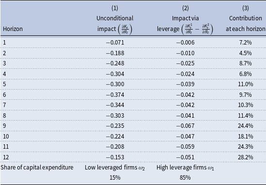
Contribution of leverage to the average investment response following recessions

Note: the table reports the coefficient at each horizon from impulse response function based on local projection methods following Jordà (Reference Jordà2005) using firm-level quarterly data from XX countries for the period 2000Q1 to 2020Q4. Estimates for the average investment response reported in column (1) are based on the regression estimated from equation (1), while estimates for the investment response of high-debt companies relative to low-debt companies are reported in column (2) are based on the regression estimated from equation (2). Column (3) estimates the contribution of high-debt companies to the decline in investment following a recessionary shock as equal to:
 $\omega _{1}\left(\frac{\partial K_{t}^{1}}{\partial R_{t}}-\frac{\partial K_{t}^{2}}{\partial R_{t}}\right)/\frac{\partial K_{t}}{\partial R_{t}}$
, assuming that group 2(low-debt companies) does not respond to the shock.
The results are robust to several checks, including to the use of various subsamples (across countries and time), alternative measures of recessions and explanatory variables, and controlling for a large set of potential cofounding factors at the macro and firm level that may be correlated with the interaction term of recession and corporate debt and affect the level of firms’ investment.
The rest of the paper is organized as follows. Section 2 presents the data and a few stylized facts. Section 3 describes the empirical methodology used to assess the (unconditional) effects of recession on firms’ investment and how it varies with the level of firms’ debt. Section 4 discusses the baseline results, Section 5 presents results for an extensive list of robustness checks, and Section 6 explores heterogeneity in results across various dimensions. Section 7 concludes.
2. Data
This section describes the data used in the paper, their sources, descriptive statistics, and key stylized facts.
2.1. Firm-level data
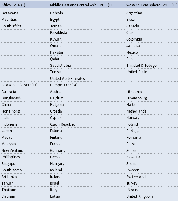
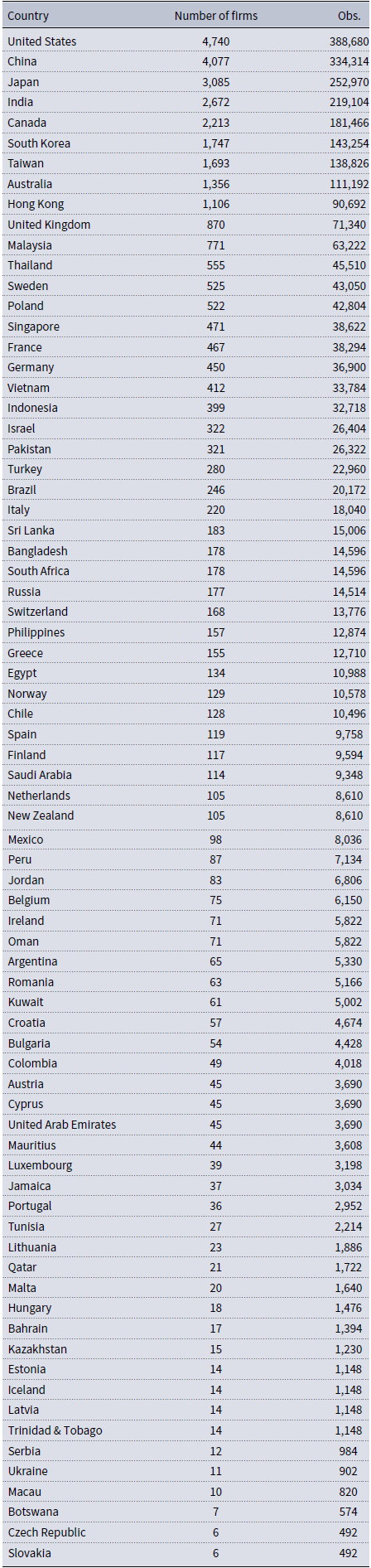
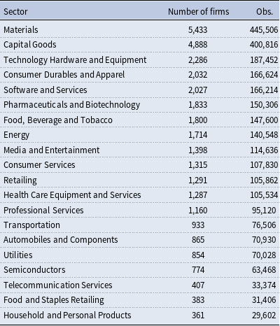
Our firm-level data comes from S&P Capital IQ. The database provides extensive balance sheet and income statement information at the firm-level and at the quarterly frequency. It covers 150 countries from 1950Q1 to 2021Q2. In order to reduce significant gaps in the time series, we restrict the sample to 2001Q1 onwards, and to advanced and emerging and developing economies. This leaves us with a sample of 75 countries. Details regarding the sample of countries used in the analysis, by geographic region, are available in Table A1 of Appendix A. The data is restricted to nonfinancial corporations and was cleaned to remove firms which had negative values for assets or debt in any year, and observations with the incorrect sign for revenue, capital expenditure, cash, tangible assets, and interest expenditure were set to missing—see Kim et al. (Reference Kim, Mano and Mrkaic2020) and Arbatli-Saxegaard et al. (Reference Arbatli-Saxegaard, Firat, Furceri and Verrier2025) for details. We further restrict the sample to exclude real estate and insurance companies. Tables A2 and A3 display the number of firms across countries and 20 economic sectors.
We make use of a set of balance sheet and cash flow statement indicators from S&P Capital IQ to investigate the evolution of firm-level investment following recession episodes, and its heterogeneity depending on firms’ characteristics—mainly focusing on firms’ debt levels.
As for our investment measure, we use capital expenditures (IQ_CAPEX-2021). This variable refers to funds used by firms to acquire assets—such as property, plant, or equipment—and generally used to undertake new investments.
Our leverage indicator measures the total amount of debt relative to assets owned by a firm. To construct this, we compute the ratio of total debt (IQ_TOTAL_DEBT-4173) to total assets (IQ_TOTAL_ASSETS - 1007). We classify each company to be high or low debt based on whether average leverage for the company over the entire sample is above or below their industries median.
We further make use of a selection of key indicators for firms’ characteristics.
Their Capital IQ code description and detailed explanation of the calculations are listed below:
-
• Total Assets (IQ_TOTAL_ASSETS - 1007).
-
• Return on Assets (IQ_RETURN_ASSETS - 4178): this metric indicates how profitable is a company in relation to its total assets.
-
• Liquidity ratio: Net working capital ratio that measures firm’s ability to pay its short-term liabilities with its current assets. The ratio is computed as the difference between current total assets (IQ_TOTAL_CA - 1008) and current total liabilities (IQ_TOTAL_CL - 1009), divided by total assets (IQ_TOTAL_ASSETS - 1007).
-
• Firm age (IQ_YEAR_FOUNDEDFootnote 7 ): Difference between the year of the observation and the year in which the firm was founded.
-
• Capital expenditure (IQ_CAPEX-2021) to lagged assets (IQ_NPPE - 1004): Ratio of capital expenditure to lagged net property, plant, and equipment. This ratio depicts how capital intensive a firm is.
-
• Revenues (IQ_TOTAL_REV-Line - 28): Revenues raised by the firm through its business activities.
-
• Firm size: Size is defined using the logarithm of total assets.
All firm level variables have been winsorized at the 1st and 99th percentiles to eliminate outliers.Footnote 8
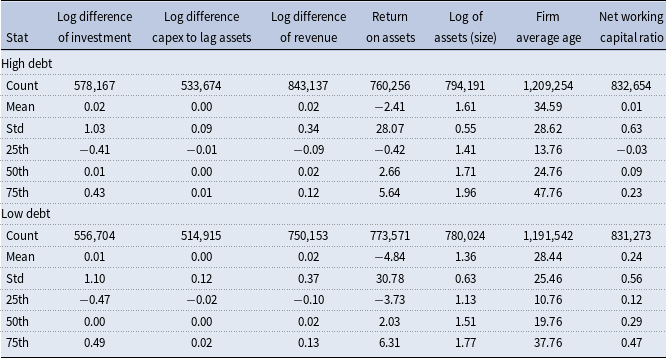
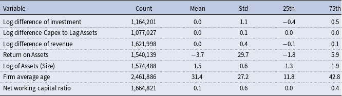
Table A4 reports summary statistics for selected firm variables, distinguishing between high- and low-debt firms. From this table, we can discern that a typical firm, independently of the level of debt, has similar characteristics in terms of changes in capital expenditure, capital expenditure to lagged assets and revenue. Moreover, highly indebted firms are larger in size, have a higher life-span and present lower liquidity. Table A5 of Appendix A reports the summary statistics of the balance sheet and cash flow statement variables used in our empirical analysis.
2.2. Recessions and other macroeconomic data
Our baseline measure for recessions is the start of a technical recession, defined by two consecutive quarters of negative GDP growth. Quarterly real gross domestic product growth from Haver Analytics is the main source used to construct this variable, but we complement it with WEO data for countries that have limited data in Haver. For these countries, we replace the full country series with WEO data. We then define a dummy where the first observation for each country’s recession episode is set to 1. This leaves us with a total of 231 recessions for AE and 336 for EM and developing economies.
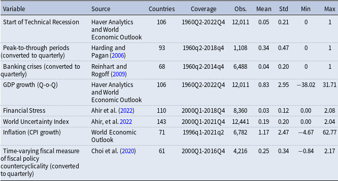
We also use two alternative measures for recession dummies: banking and financial crises (banking currency and debt) dummies from the Global Crises Data of Reinhart and Rogoff (Reference Reinhart and Rogoff2009) and peak-to-trough in GDP calculated using the Harding and Pagan (Reference Harding and Pagan2006) algorithm.Footnote 9 Recessions dummies’ data summary statistics are reported in Table A6.
2.3. Stylized Facts On Scarring and Corporate Debt
To cross-validate our firm-level investment data we compare it with investment data at the macro level. We do this for the level of investment as well as its growth rate. We first aggregate our firm-level investment variable (CAPEX) to the country-year level. To control for outliers, we first winsorize 5% tails of our firm level investment variable within each country and set investment to missing when the number of companies reporting CAPEX within a country changes abruptly.Footnote 10 Then, we calculate the countries’ annual investment growth rate as well as the log level of investment (we use USD values of investment when taking logs to make values comparable across countries).Footnote 11 We compare the log levels and growth rates of investment from the firm level dataset to aggregate investment from the WEO database. In particular, we compute these using private gross fixed capital formation from the WEO database. This variable is also converted to USD for the calculations in logarithms.
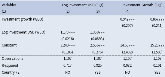
In Table A7 of Appendix A, we report the estimation results of regressing log investment from firm-level data against log-investment from macro-level data. The results show that the level of investment is highly correlated (R-squared above 0.7) across the two sources. In addition, we find that the relation between these variables remains strong and highly statistically significant when we control for country fixed effects, and when considering growth rates.
3. Empirical methodology
We use Jordà’s (Reference Jordà2005) local projection method to estimate the scarring effects of recessions and how it is amplified by the level of corporate debt at the firm level. In particular, our empirical approach consists of quantifying the short- and medium-term effect of recessions on the level of a firm’s investment. We proceed in three steps. In the first step, we estimate the average (unconditional) effect of recessions on firms’ investment. Specifically, we estimate the following specification:
 \begin{equation}y_{n,i,t+k}=\alpha _{is}^{k}+\gamma _{nq}^{k}+\sum _{j=-k}^{4}\beta _{j}^{k}R_{i,t-j}+\sum _{j=1}^{4}\theta _{j}^{k}y_{n,i,t-j}+\varepsilon _{n,i,t}^{k},\end{equation}
where dependent variable,
 $y_{n,i,t+k}$
, is the log difference of capital expenditure in firm n of country i at time (quarter) t over k quarters;
 $R_{i,t}$
is a dummy that denotes the occurrence (beginning) of an economic (technical) recession—defined as two quarters of consecutive negative GDP growth—in country i at time (quarter) t;
 $\beta _{j}^{k}$
denotes the average firm-level response of investment to recessions after k quarter.
 $\gamma_{nq}$
indicates firm-quarters dummies to control for unobservable time-unvarying firm characteristics as well as firm-specific seasonality in the level of investment;
 $\alpha _{is}^{k}$
are country-sector fixed effects to account for cross-sector variations across countries—such as country-specific comparative advantages in specific sectors. Following Teulings and Zubanov (Reference Teulings and Zubanov2014), we also include leads of the recession variable in our regressions to control for recessions that fall within the horizon of the local projection.
In the second step, we expand equation (1) to estimate how the scarring effect of recessions on the level of investment varies across firms depending on the degree of corporate debt. In particular, we estimate the following specification:
 \begin{equation}y_{n,i,t+k}=\alpha _{ist}^{k}+\gamma _{nq}^{k}+\sum _{j=-k}^{4}\mu _{j}^{k}R_{i,t-j}*D_{n}+\sum _{j=1}^{4}\theta _{j}^{k}y_{n,i,t-j}+\varepsilon _{n,i,t}^{k},\end{equation}
where D is a dummy which equals to one if the level of corporate debt associated with the firm is above the median of the industry. We use the average leverage over the entire sample to define this dummy to reduce endogeneity due to the potential time-varying response of corporate debt to recessions.
 $\alpha _{ist}^{k}$
are country-sector-time fixed effects to account for macro-economic shocks and their differential effect across sectors (such as, for example, the differential effect of recessions) as well as sector-specific shocks at the country level (such as for example, changes in country regulations affecting a given sector).Footnote
12
 $\mu _{j}^{k}$
indicates the marginal (additional) response of investment to recessions in quarter k for firms with a high (above-median) level of corporate debt relative to those with low levels of debt.
In the section of robustness checks, we consider alternative versions of equations (1)–(2) based on: changes in the definition of the recession and corporate debt dummies; different functional forms to capture how the response of firms’ investment varies with the level of debt; additional controls to include firms characteristic such as total assets, liquidity, ROA, and age; additional interaction terms to control for potential confounding factors that are correlated with recessions and/or corporate debt and that may affect the level of investment.
Equation (1)−(2) are estimated using OLS, and standard errors are two-way clustered on firm and country-time, over a panel of over 24,000 firms for the period 2001Q1 to 2020Q4 (for a total of more than 800,000 observations).
4. Results
Figure 2 presents the evolution of (log) investment following a recession episode. Time (quarter) is indicated on the x-axis; the solid line displays the average estimated response, dashed and dotted areas denote 90 and 68% confidence bands, respectively. The results suggest that recessions are associated with persistent effects on the level of investment relative to pre-recession trends. In particular, we find that the average recession in our sample is associated with a reduction in the level of investment of 30% four quarters after the recession and by 15% after 12 quarters. This effect is statistically significant and economically sizeable. The magnitude of the effect is also consistent with macro evidence on the scarring effect of recessions on investment (e.g., Furceri and Mourougane, Reference Furceri and Mourougane2012).
Evolution of (log) investment following a recession.
Note: Impulse response function based on local projection methods following Jordà (Reference Jordà2005) using firm-level quarterly data from 75 countries for the period 2001Q1 to 2020Q4. Estimates based on the regression
 $y_{n,i,t+k}=\alpha _{is}^{k}+\gamma _{nq}^{k}+\sum _{j=-\mathrm{k}}^{4}\beta _{j}^{k}R_{i,t-j}+\sum _{j=1}^{4}\theta _{j}^{k}y_{n,i,t-j}+\varepsilon _{n,i,t}^{k}$
for different horizons ‘k’, where
 $y_{n,i,t+k}$
is the log change in capital expenditure of firm n in country i at time t over the next k quarters,
 $R_{i,t-j}$
is a dummy which takes value 1 at the start of a technical recession (and is the variable of interest),
 $\gamma _{nq}^{k}$
are firm-quarters fixed effects, and
 $\alpha _{is}^{k}$
are country-sector fixed effects. The regression is estimated separately for different horizons k (for up to 12 quarters). The solid line shows the point estimate for
 $\beta _{0}^{k}$
for different horizons k, while the dotted lines are the 68 and 90% confidence intervals. Standard errors are clustered at two-way at the firm and country-time level.

Differential effect of recession on (log) investment for high-debt companies relative to low-debt companies.
Note: Impulse response function based on local projection methods following Jordà (Reference Jordà2005) using firm-level quarterly data from 75 countries for the period 2001Q1 to 2020Q4. Estimates based on the regression
 $y_{n,i,t+k}=\alpha _{ist}^{k}+\gamma _{nq}^{k}+\sum _{j=0}^{4}\mu _{j}^{k}R_{i,t-j}*D_{n}+\sum _{j=1}^{4}\theta _{j}^{k}y_{n,i,t-j}+\varepsilon _{n,i,t}^{k}$
for different horizons ‘k’, where
 $y_{n,i,t+k}$
is the log change in capital expenditure of firm n in country i at time t over the next k quarters,
 $R_{i,t-j}$
is a dummy which takes value 1 at the start of a technical recession,
 $D_{n}$
is a dummy variable if company n is a high-debt company (above median leverage within industry),
 $\gamma _{nq}^{k}$
are firm-quarters fixed effects, and
 $\alpha _{ist}^{k}$
are country-sector-time fixed effects. The regression is estimated separately for different horizons k (for up to 12 quarters). The solid line shows the point estimate for
 $\mu _{o}^{k}$
for different horizons k, while the dotted lines are the 68 and 90% confidence intervals. Standard errors are clustered at two-way at the firm and country-time level.

Figure 3 is analogous to Figure 2, but it reports the differential response of investment to recessions between a firm with relatively high corporate debt (above industry median) and firms with medium-to-low corporate debt levels. The results show that the differential investment loss for a firm with high corporate debt compared to a firm with medium-to-low corporate debt is about 2% four quarters after a recession and rises to 5% 12 quarters after. Also in this case, the effect is statistically significant and precisely estimated. Interestingly, while the average investment effects shown in Figure 2 diminish in the medium term, the differential effect for high-debt firms tend to persist. This may reflect the fact that while all firms see a large decline in investment at the start of a recession, low leverage firms may see a quicker recovery while high-debt firms see more persistent declines.
To give a sense of the role of corporate debt in amplifying the effect of recessions on investment, we perform a back-of-the-envelope calculation. We follow the approach of Arbatli-Saxegaard et al. (Reference Arbatli-Saxegaard, Firat, Furceri and Verrier2025) and Ciminelli et al. (Reference Ciminelli, Duval and Furceri2022) among others, and we use the coefficients from the estimation of equations (1)–(2) as well as the weights of firms with high corporate debt in the sample.
Since the firms in our analysis are grouped into two buckets (high leveraged firms and low leveraged firms), we can write the average response of capital expenditure as the weighted average of capital expenditure in these two groups:
 \begin{equation}K_{t=}\,\omega _{1}K_{t}^{1}+\omega _{2}K_{t}^{2}\end{equation}
where K denotes total capital expenditure,
 $\omega _{i}$
and
 $K_{t}^{i}$
are the capital expenditure share and investment of firms in group i, respectively. Based on equation (3), we can write the response of capital expenditure to recessions as follows:
 \begin{equation*}\frac{\partial K_{t}}{\partial R_{t}}=\omega _{1}\frac{\partial K_{t}^{1}}{\partial R_{t}}+\omega _{2}\frac{\partial K_{t}^{2}}{\partial R_{t}} = \omega _{1}\left(\frac{\partial K_{t}^{1}}{\partial R_{t}}-\frac{\partial K_{t}^{2}}{\partial R_{t}}\right)+\frac{\partial K_{t}^{2}}{\partial R_{t}}\end{equation*}
where
 $\omega _{2}=1-\omega _{1}$
.
We obtain
 $\frac{\partial K_{t}}{\partial R_{t}}$
from estimating equation (1), while
 $\left(\frac{\partial K_{t}^{1}}{\partial R_{t}}- \frac{\partial K_{t}^{2}}{\partial R_{t}}\right)$
from estimating equation (2). Using the coefficients from these estimations, we calculate the contribution of leverage as
 $\frac{\omega _{1}\left(\frac{\partial K_{t}^{1}}{\partial R_{t}}-\frac{\partial K_{t}^{2}}{\partial R_{t}}\right)}{\frac{\partial K_{t}}{\partial R_{t}}}$
, assuming that group 2 (
 $\frac{\partial K_{t}^{2}}{\partial R_{t}}$
) does not respond to the shock.
The results of this exercise suggest that firms’ leverage contributes significantly to the average medium-term response of firms’ investment to recessions and in amplifying scarring (Table 1). In particular, we find that firms’ debt account for about 7% of the short-term (fourth quarters ahead) response of investment to recessions and about 28% of the medium-term (12 quarters ahead) response.
5. Robustness checks
The results in the previous section highlight the role of corporate debt in amplifying the effect of recessions on firms’ investment. This section provides several robustness checks to demonstrate the generality of our results. We provide three types of checks, changing: (i) the sample; (ii) our key regressors and explanatory variable; and iii) the set of control variables to include potential cofounding factors at the macro and firm level that may be correlated with the interaction term of the recession and corporate debt dummy and that may affect the level of firms’ investment.
5.1. Sample
As a first robustness check, we examine the sensitivity of our results to alternative samples. First, we look at whether the results are driven by important episodes of corporate debt buildup such as those observed in 2009 as the outcome of the GFC and in 2020 because of COVID-19. The results reported in Figure B1 of Appendix B show that the differential response of investment for firms with high corporate debt obtained excluding these two years is similar to, and not statistically different from, the baseline. Second, we check whether the results are driven by specific countries or groups of countries. To this end, we re-estimate equation (2) by excluding one country at a time and one region at a time. The results reported in Figures B2 and B3 of Appendix B suggest that our baseline results are not driven by specific countries. Next, we repeat the analysis by excluding one 2-digit sector at a time. The results also in this case are almost unchanged compared to those reported for the full sample (Figure B4 of Appendix B). Finally, we look at whether the results are determined by influential extreme observations. To this end, we winsorize 0.05 and 5% of the tails of the distribution of our dependent variable, respectively. The results obtained are very similar to the baseline (Figure B5).
5.2. Alternative dependent variables, recessions, and debt dummies
We replicate the analysis using alternative dependent variables: (i) the ratio of capital expenditure to total lagged assets; and (ii) log of revenue. The results obtained using these variables confirm that the negative effects of recessions tend to be amplified in firms with high corporate debt (Figure B6 of Appendix B). We next look at the sensitivity of results to the definition of recessions. While our approach follows the standard in the literature and in the definition of recessions, we also consider alternative versions of recessions such as: (i) continuous GDP growth (with the sign inverted); (ii) the peak to through changes in GDP growth; (iii) a dummy for financial (banking, debt and currency) crises; and (vi) a dummy for banking crises. The results produced with these variables confirm our main findings (Figure B7). Next, we examine the robustness of the results to the way we identify firms with high corporate debt. In our baseline specification, we consider a firm to have high corporate debt if the average level of debt of the firm over the entire sample is above the median of the industry. This assumption tries to isolate the role of debt from other firms’ characteristics that may vary across sectors. As an alternative approach, we identify high-corporate-debt-firms as those with average level of debt above the median in the country or the income group specific industry median. The results reported in Figure B8 are similar to the baseline.
Robustness: exclude recessions years when computing high-debt dummy.
Note: Robustness check where companies are classified into high or low debt based on whether average leverage in all non-recession years is above or below median of their industry. Impulse response function based on local projection methods following Jordà (Reference Jordà2005) using firm-level quarterly data from 75 countries for the period 2001Q1 to 2020Q4. Estimates based on the regression
 $y_{n,i,t+k}=\alpha _{ist}^{k}+\gamma _{nq}^{k}+\sum _{j=0}^{4}\mu _{j}^{k}R_{i,t-j}*D_{n}+\sum _{j=1}^{4}\theta _{j}^{k}y_{n,i,t-j}+\varepsilon _{n,i,t}^{k}$
for different horizons ‘k’, where
 $y_{n,i,t+k}$
is the log change in capital expenditure of firm n in country i at time t over the next k quarters,
 $R_{i,t-j}$
is a dummy which takes value 1 at the start of a technical recession,
 $D_{n}$
is a dummy variable if company n is a high-debt company (above median leverage in non-recession years within industry),
 $\gamma _{nq}^{k}$
are firm-quarters fixed effects, and
 $\alpha _{ist}^{k}$
are country-sector-time fixed effects. The regression is estimated separately for different horizons k (for up to 12 quarters). The solid line shows the point estimate for
 $\mu _{o}^{k}$
for different horizons k, while the dotted lines are the 68 and 90% confidence intervals. Standard errors are clustered at two-way at the firm and country-time level.

In our baseline, to mitigate endogeneity concerns, we consider the average leverage of a company over the entire sample so firms cannot switch classification, including in response to recessions.Footnote 13 To further mitigate endogeneity, we augmented our baseline identification to exclude the recessions years in the computation of the firms’ average level of corporate debt (Figure 4). Next, we modify the way we estimate the role of firms’ debt in amplifying the effect of recessions on investment. Instead of considering an interaction between a dummy which takes value 1 if a firm’s level of debt is above the industry-median, we consider high-debt firms as those with debt level above the 4th quartile of the industry distribution. The results in Figure B9 are qualitatively similar to those obtained using the industry median as a threshold. Finally, instead of considering only one dummy, we modify equation (2) to consider two interaction terms: one between recessions and a dummy which takes value 1 for firms with level of debt above the 4th quartile of the industry distribution (high-debt firms); one between recessions and a dummy which takes value 1 for firms with level of debt below the 2nd quartile of the industry distribution (low-debt firms). In Figure B10, we report the coefficients associated with these terms for each estimation horizon. Note that each of these coefficients captures the marginal effect of being in a high (low) state of debt compared to firms with level of debt between the 2nd and the 4th quartile of the distribution. The results show that the effect of recessions on investment for firms with lower debt is always smaller compared to firms with higher debt.
5.3. Additional control variables
We augment our baseline regressions to include additional firm characteristics such as total assets, ROA, liquidity, and age. The results obtained adding these control variables do not change the baseline results (Figure B11).
Our baseline regression includes a constellation of sector-country-time fixed effects and therefore effectively controls for all macroeconomic shocks and their effect across sectors. The inclusion of firm fixed effects further controls for unobservable firm characteristics that do not vary over time. While this set of controls should reduce concerns about endogeneity, a possible concern in estimating equation (2) is that the results are biased due to the omission of macroeconomic variables affecting firm-level investment through the level of corporate debt and are at the same time correlated with our recession dummies.
The first obvious candidate is the degree of financial stress (Dell’Ariccia et al., Reference Dell Ariccia, Detragiache and Rajan2008). To check whether the inclusion of financial stress alter our results, we augment equation (2) by interacting the new indicator of financial stress from Ahir et al. (Reference Ahir, Bloom and Furceri2022) with the firms’ corporate debt dummy.Footnote 14 The results presented in the top left panel of Figure 6 show that the effect of recessions on firms’ investment through corporate debt remains of the expected sign and also statistically significant, even though the point estimates are smaller, especially in the short-term. This is because one channel through which recessions affect investment is by increasing financial stress. In addition, and in line with Ahir et al. (Reference Ahir, Bloom and Furceri2022), we also find that financial stress has a statistically significant effect on investment (Figure B12, top-left panel).Footnote 15
Uncertainty can also affect firms’ investment through corporate debt (Ahir et al. Reference Ahir, Bloom and Furceri2022; Choi et al. Reference Choi, Furceri, Huang and Loungani2018). According to these studies, fluctuations in uncertainty tend to have larger effects on firms (sectors) that are more financially constrained. To control for the role of uncertainty, we repeat the analysis by including as an additional control variable the interaction between a measure of country-specific uncertainty—The World Uncertainty Index of Ahir, et al. (Reference Ahir, Bloom and Furceri2022)—and the firm’s corporate debt dummy.Footnote 16 The effect of recessions on firms’ investment (top-left panel of Figure 6) also in this case are similar to, and not statistically different from, the baseline results presented in Figure 4. In addition, and consistent with the evidence from Ahir et al. (Reference Ahir, Bloom and Furceri2022) for sectoral data, we find that the level of investment falls after uncertainty shocks (Figure B12, top-right panel), with an even larger decline for firms with higher debt levels, which are therefore more credit-constrained (Figure B13, top-right panel).
Another variable that may affect firms’ investment through corporate debt is inflation. Inflation may lead to capital misallocation and to the extent that more financially dependent firms are those that suffer more from capital misallocation, it may have larger negative effects on firms with higher corporate debt. Moreover, inflation may affect firms’ level of investment by increasing price level uncertainty (Choi et al. Reference Choi, Furceri, Loungani and Shim2022). To further check the robustness of our results, we include an interaction term between inflation and the corporate debt dummy as a control. The results reported in the middle-left panel of Figure 6 show that effect of recession on firms’ investment via corporate debt is unchanged, while the interaction between inflation and corporate debt is negative and statistically significant for some horizons (Figure B13, bottom-left panel).
Fiscal policy can also affect firms’ investment level through high corporate debt—to the extent that expansionary fiscal policy can reduce the magnitude of recessions. In addition, Aghion et al. (Reference Aghion, Hemous and Kharroubi2014) and Choi et al. (Reference Choi, Furceri, Loungani and Shim2022) shows that an increase in a country’s degree of fiscal counter-cyclicality raises investment, and more so for industries with higher financial dependence. Also, in this case adding this control variable does not change our results (middle-right panel of Figure 6), and we do not find a significant effect of fiscal policy on investment through firms’ corporate debt (Figure B14, bottom-right panel).
Finally, the results are also robust when these four controls are included simultaneously (bottom-left panel of Figure 5).
Robustness: include interaction of macro variables with high-debt dummy.
Note: Robustness check where interaction of macro variables with high-debt dummy are included as controls. Impulse response function based on local projection methods following Jordà (Reference Jordà2005) using firm-level quarterly data from 75 countries for the period 2001Q1 to 2020Q4. Estimates based on the regression
 $y_{n,i,t+k}=\alpha _{ist}^{k}+\gamma _{nq}^{k}+\sum _{j=0}^{4}\mu _{j}^{k}R_{i,t-j}*D_{n}+\sum \nu _{j}^{k}M_{i,t-j}*D_{n}+\sum _{j=1}^{4}\theta _{j}^{k}y_{n,i,t-j}+\varepsilon _{n,i,t}^{k}$
for different horizons ‘k’, where
 $y_{n,i,t+k}$
is the log change in capital expenditure of firm n in country i at time t over the next k quarters,
 $R_{i,t-j}$
is a dummy which takes value 1 at the start of a technical recession,
 $D_{n}$
is a dummy variable if company n is a high-debt company (above median leverage in non-recession years within industry),
 $\gamma _{nq}^{k}$
are firm-quarters fixed effects, and
 $\alpha _{ist}^{k}$
are country-sector-time fixed effects. Interaction of various macro variable
 $M_{i,t-j}$
with the high-debt dummy are included as controls. The regression is estimated separately for different horizons k (for up to 12 quarters). The solid line shows the point estimate for
 $\mu _{o}^{k}$
for different horizons k, while the dotted lines are the 68 and 90% confidence intervals. Standard errors are clustered at two-way at the firm and country-time level.

Another possible concern with our results is that recessions affect firms’ investment though other firm-specific variables that are correlated with corporate debt. If this is the case, we may wrongly conclude that firms’ corporate debt is implying the scarring effect of recessions on investment when de facto other firm characteristics are at play. To address this source of omitted variable bias, we augment our specification to include the interaction between recessions and a dummy (constructed as for debt) for several firms’ characteristics: total assets, ROA, liquidity and age. The results obtained after adding these variables do not alter our finding that corporate debt is a significant factor affecting the response of investment to recessions (Figure 6). In addition, we find that the effect of recessions on investment tends to be smaller for firms with higher total assets, ROA, liquidity, and that are older, but these effects are not always precisely estimated (Figure B14).
Robustness: include interaction of recession dummy with firm characteristics.
Note: Robustness check where interaction of dummy variables for various firm characteristics and the recession variable are included as controls. Impulse response function based on local projection methods following Jordà (Reference Jordà2005) using firm-level quarterly data from 75 countries for the period 2001Q1 to 2020Q4. Estimates based on the regression
 $y_{n,i,t+k}=\alpha _{ist}^{k}+\gamma _{nq}^{k}+\sum _{j=0}^{4}\mu _{j}^{k}R_{i,t-j}*D_{n}+\sum \nu _{j}^{k}R_{i,t-j}*F_{n}+\sum _{j=1}^{4}\theta _{j}^{k}y_{n,i,t-j}+\varepsilon _{n,i,t}^{k}$
for different horizons ‘k’, where
 $y_{n,i,t+k}$
is the log change in capital expenditure of firm n in country i at time t over the next k quarters,
 $R_{i,t-j}$
is a dummy which takes value 1 at the start of a technical recession,
 $D_{n}$
is a dummy variable if company n is a high-debt company (above median leverage within industry),
 $\gamma _{nq}^{k}$
are firm-quarters fixed effects, and
 $\alpha _{ist}^{k}$
are country-sector-time fixed effects.
 $F_{n}$
is a dummy variable defined analogously to the high-debt dummy but for different firm characteristics i.e. firm classified as 1 if it is above the median as per the characteristic when averaged across the entire sample. The regression is estimated separately for different horizons k (for up to 12 quarters). The solid line shows the point estimate for
 $\mu _{o}^{k}$
for different horizons k, while the dotted lines are the 68 and 90% confidence intervals. Standard errors are clustered at two-way at the firm and country-time level.

Finally, high leverage may indicate deteriorating business health. To ensure that the observed effects are driven by high debt rather than underlying business conditions, we augment our specification by including the interaction between recessions and a dummy variable (constructed similarly to the debt dummy) based on firms’ profits. The results show that the effects for high leverage remain statistically significant and very close to the baseline when this interaction term is included (Figure 7).
Differential effect of recession on (log) investment for high-debt companies relative to low-debt companies—controlling for profitability.
Note: impulse response function based on local projection methods following Jordà (Reference Jordà2005) using firm-level quarterly data from 75 countries for the period 2001Q1 to 2020Q4. Estimates based on the regression
 $y_{n,i,t+k}=\alpha _{ist}^{k}+\gamma _{nq}^{k}+\sum _{j=0}^{4}\mu _{j}^{k}R_{i,t-j}*D_{n}+\sum _{j=1}^{4}\theta _{j}^{k}y_{n,i,t-j}+\varepsilon _{n,i,t}^{k}$
for different horizons ‘k’, where
 $y_{n,i,t+k}$
is the log change in capital expenditure of firm n in country i at time t over the next k quarters,
 $R_{i,t-j}$
is a dummy which takes value 1 at the start of a technical recession,
 $D_{n}$
is a dummy variable if company n is a high-debt company (above median leverage within industry),
 $\gamma _{nq}^{k}$
are firm-quarters fixed effects, and
 $\alpha _{ist}^{k}$
are country-sector-time fixed effects. The regression is estimated separately for different horizons k (for up to 12 quarters). The solid black line shows the point estimate for
 $\mu _{o}^{k}$
for different horizons k, while the dotted lines are the 68 and 90% confidence intervals. The solid red line indicates the baseline response reported in Figure 3. Standard errors are clustered at two-way at the firm and country-time level.

5.4. Placebo test
We next conduct a placebo test to check if investment in treated firms (i.e., highly indebted firms) behaves differently to firms in the control group even in the absence of a recession. To test this, we create 200 different random dummies with a distribution analogous to that of our original recession dummy.Footnote 17 We then rerun our baseline specification, replacing our recession dummy with the random dummies. We plot the distribution of the resulting coefficients at each horizon in Figure B15 together with the estimated coefficient in our baseline specification (vertical red line).
All the coefficients obtained using the random dummies are close to, and centered on, zero—that is, we observe no differential decrease in investment after randomly assigned placebo “recessions”. This reinforces our conclusion that firms with high debt experience larger decreases in investment after recessions compared to low-indebted firms, distinct from any other time-varying factors that might reduce their investment levels.
6. Heterogeneity
In this section, we examine the potential heterogeneity in how leverage amplifies the scarring effects of recessions. Specifically, we analyze whether the effects discussed in the previous sections are influenced by macroeconomic conditions (such as country characteristics and types of crises) as well as sector- and firm-specific factors.
6.1. Country characteristics
One macroeconomic factor that can significantly influence how leverage amplifies scarring effects is the degree of bankruptcy efficiency (Kornejew et al. Reference Kornejew, Lian, Ma, Ottonello, Perez, Kornejew, Lian, Ma, Ottonello and Perez2024). Well-functioning restructuring systems can mitigate inefficiencies arising from liquidation and help to identify viable firms—those for which the continuation value of operations exceeds the liquidation value—and restructure them effectively.
To measure the quality of a country’s bankruptcy system, we use the Strength of Insolvency Framework Index from the World Bank’s Doing Business database. This de jure indicator evaluates the extent to which a country’s laws and regulations support collective action, protect creditor rights, and facilitate efficient reorganization or liquidation. The overall index ranges from 0 to 16, with higher values indicating stronger legal provisions for resolving insolvency. The index covers 190 economies from 2004 and 2020. To test the role of a country’s bankruptcy system, we extend equation (2) as follows:
 \begin{eqnarray}y_{n,i,t+k}&=&\alpha _{ist}^{k}+\gamma _{nq}^{k}+\sum _{j=-k}^{4}\mu _{j}^{k}R_{i,t-j}*D_{n}+\sum _{j=-k}^{4}\sigma _{j}^{k}R_{i,t-j}*D_{n}*Z_{i,t-1}\nonumber\\&&+\sum \delta _{j}^{k}D_{n}*Z_{i,t-1}+\sum _{j=1}^{4}\theta _{j}^{k}y_{n,i,t-j}+\varepsilon _{n,i,t}^{k},\end{eqnarray}
where
 $Z_{i,t-1}$
is a dummy which takes value 1 if the efficiency score is above the sample median and zero otherwise. The coefficient on the triple interaction term
 $\sigma _{j}^{k}$
measures whether the differential response of investment for high-debt firms in quarter k varies based on the country’s degree of bankruptcy efficiency. The results reported in Panel A of Figure 8 suggest that the coefficient is positive and statistically significant in the medium term, indicating that the differential scarring effects for high-leverage firms are markedly lower in countries with more efficient bankruptcy systems.
Differential effect of recession on (log) investment for high-debt companies relative to low-debt companies—role of bankruptcy efficiency.
Note: Impulse response function based on local projection methods following Jordà (Reference Jordà2005) using firm-level quarterly data from 75 countries for the period 2001Q1 to 2020Q4. Estimates based on the regression
 $y_{n,i,t+k}=\alpha_{ist}^{k}+\gamma_{nq}^{k} + \sum_{j=-\mathrm{k}}^{4}\mu^{k}_{j} R_{i,t-j}\ast D_{n} + \sum_{j=-k}^{4} \sigma_{j}^{k} R_{i,t-j} \ast D_{n} \ast Z_{i,t-1} + \sum\delta^{k}_{j} D_{n}*Z_{i,t-1}+\sum^{4}_{j=1} \theta^{k}_{j} y_{n,i,t-j} + \varepsilon^{k}_{n,i,t}$
for different horizons ‘k’, where
 $y_{n,i,t+k}$
is the log change in capital expenditure of firm n in country i at time t over the next k quarters,
 $R_{i,t-j}$
is a dummy which takes value 1 at the start of a technical recession,
 $D_{n}$
is a dummy variable if company
 $n$
is a high-debt company (above median leverage within industry),
 $Z_{i,t-1}$
is an indicator of bankruptcy efficiency,
 $\lambda^{k}_{nd}$
are firm-quarters fixed effects, and
 $\alpha^{k}_{ist}$
are country-sector-time fixed effects. The regression is estimated separately for different horizons k (for up to 12 quarters). The solid black line shows the point estimate for
 $\mu^{k}_{o}$
for different horizons k, while the dotted lines are the 68 percent and 90 percent confidence intervals. The solid red line indicates the baseline response reported in Figure 3. Standard errors are clustered at two-way at the firm and country-time level.

AE are generally characterized by a higher level of bankruptcy efficiency (Figure A1). A potential concern is that the results in Panel A of Figure 8 may simply reflect the differential response of scarring across income groups. To address this possibility, we re-estimated equation (4) separately for AE and EM economies. The results presented in Panel B of Figure 8 indicate that, for each income group, the differential scarring effects for high-leverage firms are smaller in countries with stronger bankruptcy institutions. These results indicate that bankruptcy efficiency is an independent factor influencing scarring, separate from the level of income.
6.2. Types of recessions
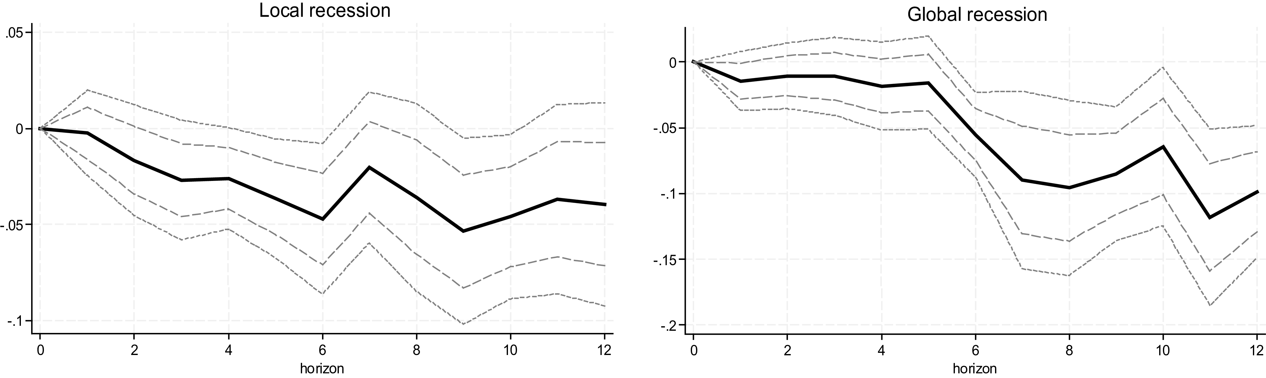
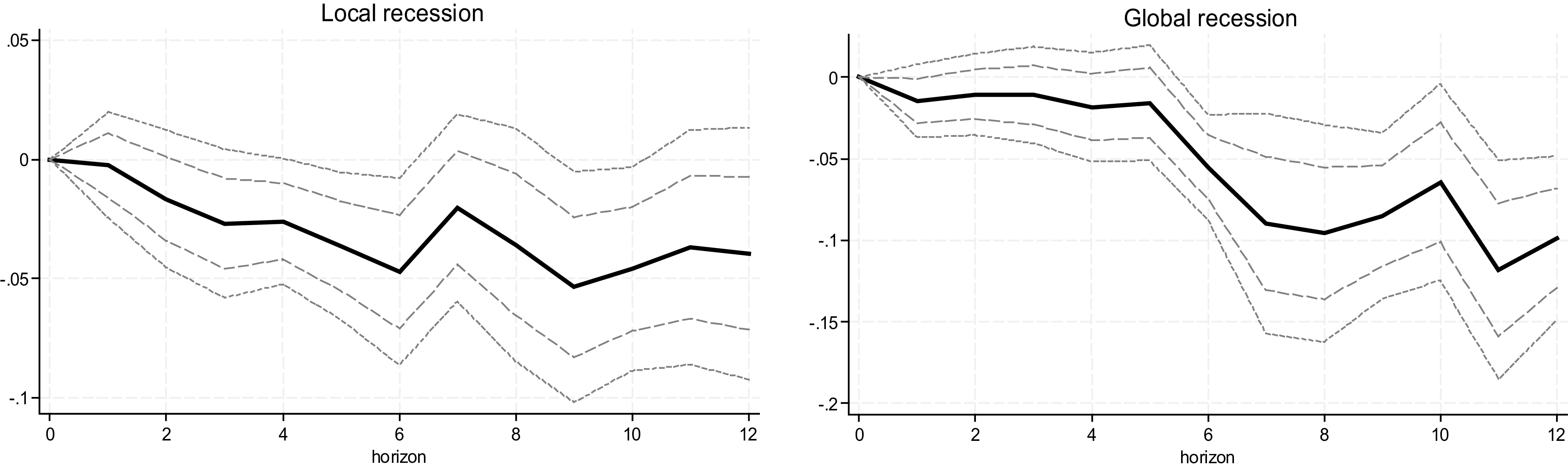
Our sample encompasses two major global recessions: the GFC and the Covid-19 pandemic. These crises have been notable not only for their scarring effects but also for the tighter financial conditions they have created. Both factors are likely to amplify the long-term effect of recessions on investment through leverage. To assess the differential impact of these global recessions, we re-estimated equation (2) for both global and domestic recessions. The results presented in Figure 9 indicate that the differential scarring effects for high-debt firms are approximately twice as large during global recessions compared to domestic ones.
Differential effect of recession on (log) investment for high-debt companies relative to low-debt companies—global vs. domestic recessions.
Note: Impulse response function based on local projection methods following Jordà (Reference Jordà2005) using firm-level quarterly data from 75 countries for the period 2001Q1 to 2020Q4. Estimates based on the regression
 $y_{n,i,t+k}=\alpha _{ist}^{k}+\gamma _{nq}^{k}+\sum _{j=0}^{4}\mu _{j}^{k}R_{i,t-j}*D_{n}+\sum _{j=1}^{4}\theta _{j}^{k}y_{n,i,t-j}+\varepsilon _{n,i,t}^{k}$
for different horizons ‘k’, where
 $y_{n,i,t+k}$
is the log change in capital expenditure of firm n in country i at time t over the next k quarters,
 $R_{i,t-j}$
is a dummy which takes value 1 at the start of a technical recession,
 $D_{n}$
is a dummy variable if company n is a high-debt company (above median leverage within industry),
 $\gamma _{nq}^{k}$
are firm-quarters fixed effects, and
 $\alpha _{ist}^{k}$
are country-sector-time fixed effects. The regression is estimated separately for different horizons k (for up to 12 quarters). The solid black line shows the point estimate for
 $\mu _{o}^{k}$
for different horizons k, while the dotted lines are the 68 and 90% confidence intervals. The solid red line indicates the baseline response reported in Figure 3. Standard errors are clustered at two-way at the firm and country-time level.

6.3. Sectoral and firm characteristics
Global and domestic recessions are likely to affect firms differently, depending on the extent of their trade exposure. Data limitations hinder our ability to exploit firm-level heterogeneity regarding the trade channel. While CIQ provides export revenue data for firms, its coverage is quite limited. To address this limitation, and following Arbatli-Saxegaard et al. (Reference Arbatli-Saxegaard, Firat, Furceri and Verrier2025), we use the World Input–Output Database (WIOD) as our baseline, which offers cross-country trade data for 56 sectors in 43 countries from 2000 to 2014.Footnote
18
We calculate the average export dependence for each sector-country pair during this period such that:
 $\textit{ExportDependenc}e_{cs}=\frac{\textit{Export}s_{cs}}{\textit{Outpu}t_{cs}}$
where c and s denote country and sector, respectively.
 $\textit{ExportDependenc}e_{cs}$
denotes the average share of exports (
 $\textit{Export}s_{cs}$
) in sector s and country c in the value of total output (
 $\textit{Outpu}t_{cs}$
).
To test for the role of trade dependency, we segment equation (2) as follows:
 \begin{eqnarray}y_{n,i,t+k}&=&\alpha _{ist}^{k}+\gamma _{nq}^{k}+\sum _{j=-k}^{4}\mu _{j}^{k}R_{i,t-j}*D_{n}+\sum _{j=-k}^{4}\sigma _{j}^{k}R_{i,t-j}*D_{n}*M_{i,s,t-1}\nonumber\\&&+\sum \delta _{j}^{k}D_{n}*M_{i,s,t-1}+\sum _{j=1}^{4}\theta _{j}^{k}y_{n,i,t-j}+\varepsilon _{n,i,t}^{k},\end{eqnarray}
where
 $M_{i,s,t-1}$
is a dummy variable which take value 1 for sectors that have above average export dependency and zero otherwise. The coefficient on the triple interaction term
 $\sigma _{j}^{k}$
measures whether the differential response of investment for high-debt firms in quarter k varies depending on the extent of export dependence. The results presented in Figure 10 for global and domestic recessions confirm that the differential scarring effects for global (domestic) recessions are larger (smaller) for firms in sectors characterized by higher export dependence.
Differential effect of recession on (log) investment for high-debt companies relative to low-debt companies—global vs. domestic recessions and export dependence.
Note: Impulse response function based on local projection methods following Jordà (Reference Jordà2005) using firm-level quarterly data from 75 countries for the period 2001Q1 to 2020Q4. Estimates based on the regression
 $y_{n,i,t+k}=\alpha _{ist}^{k}+\gamma _{nq}^{k}+\sum _{j=-k}^{4}\mu _{j}^{k}R_{i,t-j}*D_{n}+\sum _{j=-k}^{4}\sigma _{j}^{k}R_{i,t-j}*D_{n}*M_{i,s,t-1}+\sum \delta _{j}^{k}D_{n}*Z_{i,s,t-1}+\sum _{j=1}^{4}\theta _{j}^{k}y_{n,i,t-j}+\varepsilon _{n,i,t}^{k}$
for different horizons ‘k’, where
 $y_{n,i,t+k}$
is the log change in capital expenditure of firm n in country i at time t over the next k quarters,
 $R_{i,t-j}$
is a dummy which takes value 1 at the start of a technical recession,
 $D_{n}$
is a dummy variable if company n is a high-debt company (above median leverage within industry),
 $M_{i,s,t-1}$
is a dummy for high export dependence,
 $\gamma _{nq}^{k}$
are firm-quarters fixed effects, and
 $\alpha _{ist}^{k}$
are country-sector-time fixed effects. The regression is estimated separately for different horizons k (for up to 12 quarters). The solid black line shows the point estimate for
 $\mu _{o}^{k}$
for different horizons k, while the dotted lines are the 68 and 90% confidence intervals. The solid red line indicates the baseline response reported in Figure 3. Standard errors are clustered at two-way at the firm and country-time level.

Differential effect of recession on (log) investment for high-debt companies relative to low-debt companies—firms characteristics.
Note: Impulse response function based on local projection methods following Jordà (Reference Jordà2005) using firm-level quarterly data from 75 countries for the period 2001Q1 to 2020Q4. Estimates based on equation (3) for different horizons ‘k’. The solid line shows the point estimate for
 $\nu _{o}^{k}$
, the coefficient on the triple interaction term, for different horizons k, while the dotted lines are the 68% and 90% confidence intervals. Standard errors are clustered at two-way at the firm and country-time level.

Finally, in the third step, we further expand equation (2) to test whether the differential effect of recessions on investment for high-debt firms depends on other firm characteristics. In particular, we estimate the following triple-interaction specification:
 \begin{eqnarray}y_{n,i,t+k}&=&\alpha _{ist}^{k}+\gamma _{nq}^{k}+\sum _{j=-k}^{4}\mu _{j}^{k}R_{i,t-j}*D_{n}+\sum _{j=-k}^{4}\nu _{j}^{k}R_{i,t-j}*D_{n}*X_{n,i,t-1}+\sum \beta _{j}^{k}R_{i,t-j}*X_{n,i,t-1}\nonumber\\&&+\sum \delta _{j}^{k}D_{n}*X_{n,i,t-1}+\sum _{j=1}^{4}\theta _{j}^{k}y_{n,i,t-j}+\varepsilon _{n,i,t}^{k},\end{eqnarray}
where
 $X_{n,i,t-1}$
is the lagged value (averaged over four quarters to reduce noise) of a firm level characteristic like size, profitability, or share of short-term debt. The coefficient on the triple interaction term
 $\nu _{j}^{k}$
measures whether the differential response of investment for high-debt firms in quarter k varies depending on the firm characteristic
 $X_{n,i,t-1}$
.
First, we test the impact of firm size measured by the log of total assets. We find that the coefficient on the triple interaction term in equation (3) is positive and significant (Figure 11A), indicating that larger firms with high debt see less scarring in investment following recessions compared to smaller firms with high debt. This could reflect the fact that for a given level of debt, credit constraints are more binding for smaller firms than larger firms, potentially because larger firms have more collateral available for borrowing, or because lenders see larger firms as less risky compared to smaller firms (Ghosal and Loungani, Reference Ghosal and Loungani2000; Cloyne et al. Reference Cloyne, Huber, Ilzetzki and Kleven2019; Arbatli-Saxegaard et al. Reference Arbatli-Saxegaard, Firat, Furceri and Verrier2025). Therefore, larger firms even with high debt are better positioned to take advantage of investment opportunities following a recession compared to similar smaller firms.
Next, we test whether profitability, measured using return on assets, also impacts the differential effect on investment of high- versus low-debt firms following a recession. We find that the triple interaction term when using return on assets is also positive and significant at longer horizons (Figure 11B), indicating that more profitable firms with high debt see less scarring compared to less profitable firms. This could reflect the fact that more profitable firms have greater access to internal funds to finance investment activities, thus relaxing credit constraints faced by less profitable high-debt firms.
Finally, we test whether the differential effect on investment of high- versus low-debt firms following a recession depends on the maturity structure of the firms’ debt. The hypothesis we want to test is that it is harder for high short-term debt firms to rollover it in the aftermath of a recession, thus making it more difficult for them to invest in new projects. Our results suggest that this is the case, and we find that the triple interaction term when using share of short-term debt is negative (Figure 11C), indicating that companies with shorter maturity structures of debt see more scarring compared to those with longer maturities.
Appendix Figure B16 checks the robustness of the triple interaction results to using a smooth transition function (Granger and Terävistra, Reference Granger and Teräsvirta1993) to transform the size and return on assets variable before estimating the triple interaction. The results are robust to this alternative specification and generally more precisely estimated. In contrast, we did not find statistically significant effects for triple interactions with other variables commonly used in the literature to proxy financial constraints such as age and liquidity. While the signs of the estimated effects are consistent with those obtained for size and profitability—that is, the differential investment effect between high- and low-debt firms is larger for younger and less liquid firms—these effects are not precisely estimated.
7. Conclusions
Corporate debt has increased markedly in the last two decades in both AE and EM economies. In this paper, we show that this rising trend will reduce the resilience of economies to recessionary shocks, other things equal. In particular, applying Jordà’s (Reference Jordà2005) local projection methods to a large panel of more than 24,000 firms, we find that the recessionary shocks that occurred during the period 2001–2020 have resulted in significant and persistent drops in investment, with the effects being larger for firms with higher debt. The effect of firms’ leverage in shaping the investment response to recessions is statistically significant, and robust to a wide range of sensitivity checks. It is also economically sizeable: back-of-the-envelope calculations suggest that firms’ debt accounts for at least 28% of the average medium-term response of investment to recessions.
These effects are larger for countries with less efficient bankruptcy systems, and tend to be amplified during global recessions—especially for firms operating in sectors with higher export dependence. In addition, we find that these effects are larger for smaller and less profitable firms, suggesting that for a given level of debt, credit constraints are more binding for smaller firms than larger firms, potentially because larger firms have more collateral available for borrowing, or because lenders see larger firms as less risky compared to smaller firms. Moreover, we find that it is harder for high short-term debt firms to rollover debt in the aftermath of a recession, thus making it more difficult for them to invest in new projects.
Our results have important policy implications. They point to the need to adopt improved policy regimes for restructuring unviable firms (see Grigorian and Raei, Reference Grigorian and Raei2010 for lessons from the GFC), avoid firms’ zombification, reduce overall leverage at the country-level and promote reallocation of capital and labor toward the more productive firms.
Acknowledgments
We thank participants in various conferences and universities for their valuable comments and suggestions. The views expressed in this paper are those of the authors and should not be attributed to the views of the IMF, its Executive Board, or IMF management.
Appendix A. Data
Sample of 75 countries by region

Number of firms and observations by country

Number of firms and observations by sector

Summary statistics by leverage

Summary statistics of firm-level database

Summary statistics of macroeconomic variables

Correlation of investment between Capital IQ and World Economic Outlook data

Robust standard errors in parentheses.
*** p < 0.01, ** p < 0.05, * p < 0.1.
Bankruptcy efficiency in advanced economies (AE) and emerging markets (EM).
Source: World Bank.

Appendix B. Additional results
Robustness: excluding GFC and COVID-19.
Note: Left panel excludes the year 2009 from the estimation while the right panel excludes the year 2020. Impulse response function based on local projection methods following Jordà (Reference Jordà2005) using firm-level quarterly data from 75 countries for the period 2001Q1 to 2020Q4. Estimates based on the regression
 $y_{n,i,t+k}=\alpha _{ist}^{k}+\gamma _{nq}^{k}+\sum _{j=0}^{4}\mu _{j}^{k}R_{i,t-j}*D_{n}+\sum _{j=1}^{4}\theta _{j}^{k}y_{n,i,t-j}+\varepsilon _{n,i,t}^{k}$
for different horizons ‘k’, where
 $y_{n,i,t+k}$
is the log change in capital expenditure of firm n in country i at time t over the next k quarters,
 $R_{i,t-j}$
is a dummy which takes value 1 at the start of a technical recession,
 $D_{n}$
is a dummy variable if company n is a high-debt company (above median leverage within industry),
 $\gamma _{nq}^{k}$
are firm-quarters fixed effects, and
 $\alpha _{ist}^{k}$
are country-sector-time fixed effects. The regression is estimated separately for different horizons k (for up to 12 quarters). The solid line shows the point estimate for
 $\mu _{o}^{k}$
for different horizons k, while the dotted lines are the 68 and 90% confidence intervals. Standard errors are clustered at two-way at the firm and country-time level.

Robustness: excluding countries with most observations.
Note: Each impulse response checks robustness to excluding one country from the baseline regression—the 10 countries with the most observations in the sample are excluded one at a time. Impulse response function based on local projection methods following Jordà (Reference Jordà2005) using firm-level quarterly data from 75 countries for the period 2001Q1 to 2020Q4. Estimates based on the regression
 $y_{n,i,t+k}=\alpha _{ist}^{k}+\gamma _{nq}^{k}+\sum _{j=0}^{4}\mu _{j}^{k}R_{i,t-j}*D_{n}+\sum _{j=1}^{4}\theta _{j}^{k}y_{n,i,t-j}+\varepsilon _{n,i,t}^{k}$
for different horizons ‘k’, where
 $y_{n,i,t+k}$
is the log change in capital expenditure of firm n in country i at time t over the next k quarters,
 $R_{i,t-j}$
is a dummy which takes value 1 at the start of a technical recession,
 $D_{n}$
is a dummy variable if company n is a high-debt company (above median leverage within industry),
 $\gamma _{nq}^{k}$
are firm-quarters fixed effects, and
 $\alpha _{ist}^{k}$
are country-sector-time fixed effects. The regression is estimated separately for different horizons k (for up to 12 quarters). The solid line shows the point estimate for
 $\mu _{o}^{k}$
for different horizons k, while the dotted lines are the 68 and 90% confidence intervals. Standard errors are clustered at two-way at the firm and country-time level.

Robustness: excluding one region at a time.
Note: Each impulse response checks robustness to excluding one region at a time. Impulse response function based on local projection methods following Jordà (Reference Jordà2005) using firm-level quarterly data from 75 countries for the period 2001Q1 to 2020Q4. Estimates based on the regression
 $y_{n,i,t+k}=\alpha _{ist}^{k}+\gamma _{nq}^{k}+\sum _{j=0}^{4}\mu _{j}^{k}R_{i,t-j}*D_{n}+\sum _{j=1}^{4}\theta _{j}^{k}y_{n,i,t-j}+\varepsilon _{n,i,t}^{k}$
for different horizons ‘k’, where
 $y_{n,i,t+k}$
is the log change in capital expenditure of firm n in country i at time t over the next k quarters,
 $R_{i,t-j}$
is a dummy which takes value 1 at the start of a technical recession,
 $D_{n}$
is a dummy variable if company n is a high-debt company (above median leverage within industry),
 $\gamma _{nq}^{k}$
are firm-quarters fixed effects, and
 $\alpha _{ist}^{k}$
are country-sector-time fixed effects. The regression is estimated separately for different horizons k (for up to 12 quarters). The solid line shows the point estimate for
 $\mu _{o}^{k}$
for different horizons k, while the dotted lines are the 68 and 90% confidence intervals. Standard errors are clustered at two-way at the firm and country-time level.

Robustness: excluding one sector at a time.
Note: Each impulse response checks robustness to excluding one 2-digit sector at a time. Impulse response function based on local projection methods following Jordà (Reference Jordà2005) using firm-level quarterly data from 75 countries for the period 2001Q1 to 2020Q4. Estimates based on the regression
 $y_{n,i,t+k}=\alpha _{ist}^{k}+\gamma _{nq}^{k}+\sum _{j=0}^{4}\mu _{j}^{k}R_{i,t-j}*D_{n}+\sum _{j=1}^{4}\theta _{j}^{k}y_{n,i,t-j}+\varepsilon _{n,i,t}^{k}$
for different horizons ‘k’, where
 $y_{n,i,t+k}$
is the log change in capital expenditure of firm n in country i at time t over the next k quarters,
 $R_{i,t-j}$
is a dummy which takes value 1 at the start of a technical recession,
 $D_{n}$
is a dummy variable if company n is a high-debt company (above median leverage within industry),
 $\gamma _{nq}^{k}$
are firm-quarters fixed effects, and
 $\alpha _{ist}^{k}$
are country-sector-time fixed effects. The regression is estimated separately for different horizons k (for up to 12 quarters). The solid line shows the point estimate for
 $\mu _{o}^{k}$
for different horizons k, while the dotted lines are the 68 and 90% confidence intervals. Standard errors are clustered at two-way at the firm and country-time level.

Robustness: different winsorizing schemes.
Note: Left panel winsorizes 0.05 percent tails of the dependent variable while the right panel winsorizes 5% tails of the dependent variable (compared to the baseline which winsorizes 1 percent tails). Impulse response function based on local projection methods following Jordà (Reference Jordà2005) using firm-level quarterly data from 75 countries for the period 2001Q1 to 2020Q4. Estimates based on the regression
 $y_{n,i,t+k}=\alpha _{ist}^{k}+\gamma _{nq}^{k}+\sum _{j=0}^{4}\mu _{j}^{k}R_{i,t-j}*D_{n}+\sum _{j=1}^{4}\theta _{j}^{k}y_{n,i,t-j}+\varepsilon _{n,i,t}^{k}$
for different horizons ‘k’, where
 $y_{n,i,t+k}$
is the log change in capital expenditure of firm n in country i at time t over the next k quarters,
 $R_{i,t-j}$
is a dummy which takes value 1 at the start of a technical recession,
 $D_{n}$
is a dummy variable if company n is a high-debt company (above median leverage within industry),
 $\gamma _{nq}^{k}$
are firm-quarters fixed effects, and
 $\alpha _{ist}^{k}$
are country-sector-time fixed effects. The regression is estimated separately for different horizons k (for up to 12 quarters). The solid line shows the point estimate for
 $\mu _{o}^{k}$
for different horizons k, while the dotted lines are the 68 and 90% confidence intervals. Standard errors are clustered at two-way at the firm and country-time level.

Robustness: different dependent variables.
Note: Impulse response function based on local projection methods following Jordà (Reference Jordà2005) using firm-level quarterly data from 75 countries for the period 2001Q1 to 2020Q4. Estimates based on the regression
 $y_{n,i,t+k}=\alpha _{ist}^{k}+\gamma _{nq}^{k}+\sum _{j=0}^{4}\mu _{j}^{k}R_{i,t-j}*D_{n}+\sum _{j=1}^{4}\theta _{j}^{k}y_{n,i,t-j}+\varepsilon _{n,i,t}^{k}$
for different horizons ‘k’, where
 $y_{n,i,t+k}$
is the log change in capital expenditure of firm n in country i at time t over the next k quarters,
 $R_{i,t-j}$
is a dummy which takes value 1 at the start of a technical recession,
 $D_{n}$
is a dummy variable if company n is a high-debt company (above median leverage within industry),
 $\gamma _{nq}^{k}$
are firm-quarters fixed effects, and
 $\alpha _{ist}^{k}$
are country-sector-time fixed effects. The regression is estimated separately for different horizons k (for up to 12 quarters). The solid line shows the point estimate for
 $\mu _{o}^{k}$
for different horizons k, while the dotted lines are the 68 and 90% confidence intervals. Standard errors are clustered at two-way at the firm and country-time level.

Robustness: alternate recessions variables.
Note: Impulse response function based on local projection methods following Jordà (Reference Jordà2005) using firm-level quarterly data from 75 countries for the period 2001Q1 to 2020Q4. Estimates based on the regression
 $y_{n,i,t+k}=\alpha _{ist}^{k}+\gamma _{nq}^{k}+\sum _{j=0}^{4}\mu _{j}^{k}R_{i,t-j}*D_{n}+\sum _{j=1}^{4}\theta _{j}^{k}y_{n,i,t-j}+\varepsilon _{n,i,t}^{k}$
for different horizons ‘k’, where
 $y_{n,i,t+k}$
is the log change in capital expenditure of firm n in country i at time t over the next k quarters,
 $R_{i,t-j}$
is a dummy which takes value 1 to denote a recession,
 $D_{n}$
is a dummy variable if company n is a high-debt company (above median leverage within industry),
 $\gamma _{nq}^{k}$
are firm-quarters fixed effects, and
 $\alpha _{ist}^{k}$
are country-sector-time fixed effects. The regression is estimated separately for different horizons k (for up to 12 quarters). The solid line shows the point estimate for
 $\mu _{o}^{k}$
for different horizons k, while the dotted lines are the 68 and 90% confidence intervals. Standard errors are clustered at two-way at the firm and country-time level. Periods of banking crises are identified as the quarters during which a banking crisis-led recession occurred. Periods of peaks and troughs in economic activity are identified using the Harding-Pagan algorithm applied to real GDP. Periods of negative growth correspond to those where quarterly real GDP growth was negative.

Robustness: alternate debt dummies.
Note: Impulse response functions based on local projection methods following Jordà (Reference Jordà2005) using firm-level quarterly data from 75 countries for the period 2001Q1 to 2020Q4. Estimates based on the regression
 $y_{n,i,t+k}=\alpha _{ist}^{k}+\gamma _{nq}^{k}+\sum _{j=0}^{4}\mu _{j}^{k}R_{i,t-j}*D_{n}+\sum _{j=1}^{4}\theta _{j}^{k}y_{n,i,t-j}+\varepsilon _{n,i,t}^{k}$
for different horizons ‘k’, where
 $y_{n,i,t+k}$
is the log change in capital expenditure of firm n in country i at time t over the next k quarters,
 $R_{i,t-j}$
is a dummy which takes value 1 to denote a recession,
 $D_{n}$
is a dummy variable if company n is a high-debt company. A high-debt company is identified if its leverage is above the median leverage within country (left-hand graph), or above the median leverage within countries that are advanced economies or EMDEs respectively (right-hand graph).
 $\gamma _{nq}^{k}$
are firm-quarters fixed effects, and
 $\alpha _{ist}^{k}$
are country-sector-time fixed effects. The regression is estimated separately for different horizons k (for up to 12 quarters). The solid line shows the point estimate for
 $\mu _{o}^{k}$
for different horizons k, while the dotted lines are the 68 and 90% confidence intervals. Standard errors are clustered at two-way at the firm and country-time level.

Robustness: alternate specifications for high-debt dummies II.
Note: Impulse response functions based on local projection methods following Jordà (Reference Jordà2005) using firm-level quarterly data from 75 countries for the period 2001Q1 to 2020Q4. Estimates based on the regression
 $y_{n,i,t+k}=\alpha _{ist}^{k}+\gamma _{nq}^{k}+\sum _{j=0}^{4}\mu _{j}^{k}R_{i,t-j}*D_{n}+\sum _{j=1}^{4}\theta _{j}^{k}y_{n,i,t-j}+\varepsilon _{n,i,t}^{k}$
for different horizons ‘k’, where
 $y_{n,i,t+k}$
is the log change in capital expenditure of firm n in country i at time t over the next k quarters,
 $R_{i,t-j}$
is a dummy which takes value 1 to denote a recession,
 $D_{n}$
is a dummy variable if company n is a high-debt company. A high-debt company is identified if its leverage is above the highest tercile (quartile) leverage within industry.
 $\gamma _{nq}^{k}$
are firm-quarters fixed effects, and
 $\alpha _{ist}^{k}$
are country-sector-time fixed effects. The regression is estimated separately for different horizons k (for up to 12 quarters). The solid line shows the point estimate for
 $\mu _{o}^{k}$
for different horizons k, while the dotted lines are the 68 and 90% confidence intervals. Standard errors are clustered at two-way at the firm and country-time level.

Alternative high-debt specification: companies in the 2nd quartiles vs companies in the 4th quartile.
Note: Impulse response functions based on local projection methods following Jordà (Reference Jordà2005) using firm-level quarterly data from 75 countries for the period 2001Q1 to 2020Q4. Estimates based on the regression
 $y_{n,i,t+k}=\alpha _{ist}^{k}+\gamma _{nq}^{k}+\sum _{j=0}^{4}\mu _{j}^{k}R_{i,t-j}*D_{n}+\sum _{j=1}^{4}\theta _{j}^{k}y_{n,i,t-j}+\varepsilon _{n,i,t}^{k}$
for different horizons ‘k’, where
 $y_{n,i,t+k}$
is the log change in capital expenditure of firm n in country i at time t over the next k quarters,
 $R_{i,t-j}$
is a dummy which takes value 1 to denote a recession,
 $D_{n}$
is a dummy variable if company n is a high-debt company. A high (low) debt company is identified if its leverage is above (below) the highest (second) quartile leverage within industry.
 $\gamma _{nq}^{k}$
are firm-quarters fixed effects, and
 $\alpha _{ist}^{k}$
are country-sector-time fixed effects. The regression is estimated separately for different horizons k (for up to 12 quarters). The solid line shows the point estimate for
 $\mu _{o}^{k}$
for different horizons k, while the dotted lines are the 68 and 90% confidence intervals. Standard errors are clustered at two-way at the firm and country-time level.

Robustness: additional firm-level controls.
Note: Robustness to adding firm level controls to the baseline. Impulse response function based on local projection methods following Jordà (Reference Jordà2005) using firm-level quarterly data from 75 countries for the period 2001Q1 to 2020Q4. Estimates based on the regression
 $y_{n,i,t+k}=\alpha _{ist}^{k}+\gamma _{nq}^{k}+\sum _{j=0}^{4}\mu _{j}^{k}R_{i,t-j}*D_{n}+\sum _{j=1}^{4}\theta _{j}^{k}y_{n,i,t-j}+\sum _{j=1}^{4}\theta _{j}^{k}x_{n,i,t-j}+\varepsilon _{n,i,t}^{k}$
for different horizons ‘k’, where
 $y_{n,i,t+k}$
is the log change in capital expenditure of firm n in country i at time t over the next k quarters,
 $R_{i,t-j}$
is a dummy which takes value 1 at the start of a technical recession,
 $D_{n}$
is a dummy variable if company n is a high-debt company (above median leverage within industry),
 $\gamma _{nq}^{k}$
are firm-quarters fixed effects, and
 $\alpha _{ist}^{k}$
are country-sector-time fixed effects.
 $x_{n,i,t}$
are additional firm level controls. Left panel includes lags of firm size (ln assets), return on assets, and a measure of liquidity (current assets minus liabilities as a share of assets) as additional controls. The right panel also adds log revenues and the firms age as controls. The regression is estimated separately for different horizons k (for up to 12 quarters). The solid line shows the point estimate for
 $\mu _{o}^{k}$
for different horizons k, while the dotted lines are the 68 and 90% confidence intervals. Standard errors are clustered at two-way at the firm and country-time level.

Unconditional response of log (investment) to macro variables.
Note: Impulse response function based on local projection methods following Jordà (Reference Jordà2005) using firm-level quarterly data from 75 countries for the period 2001Q1 to 2020Q4. Estimates based on the regression
 $y_{n,i,t+k}=\alpha _{is}^{k}+\gamma _{nq}^{k}+\sum _{j=0}^{4}\beta _{j}^{k}M_{i,t-j}+\sum _{j=1}^{4}\theta _{j}^{k}y_{n,i,t-j}+\varepsilon _{n,i,t}^{k}$
for different horizons ‘k’, where
 $y_{n,i,t+k}$
is the log change in capital expenditure of firm n in country i at time t over the next k quarters,
 $M_{i,t-j}$
is different macro variable in different panels,
 $\gamma _{nq}^{k}$
are firm-quarters fixed effects, and
 $\alpha _{is}^{k}$
are country-sector fixed effects. The regression is estimated separately for different horizons k (for up to 12 quarters). The solid line shows the point estimate for
 $\beta _{0}^{k}$
for different horizons k, while the dotted lines are the 68 and 90% confidence intervals. Standard errors are clustered at two-way at the firm and country-time level.

Coefficients on interaction of macro variables with high-debt dummy as controls.
Note: Robustness check where interaction of macro variables with high-debt dummy are included as controls. Impulse response function based on local projection methods following Jordà (Reference Jordà2005) using firm-level quarterly data from 75 countries for the period 2001Q1 to 2020Q4. Estimates based on the regression
 $y_{n,i,t+k}=\alpha _{ist}^{k}+\gamma _{nq}^{k}+\sum _{j=0}^{4}\mu _{j}^{k}R_{i,t-j}*D_{n}+\sum \nu _{j}^{k}M_{i,t-j}*D_{n}+\sum _{j=1}^{4}\theta _{j}^{k}y_{n,i,t-j}+\varepsilon _{n,i,t}^{k}$
for different horizons ‘k’, where
 $y_{n,i,t+k}$
is the log change in capital expenditure of firm n in country i at time t over the next k quarters,
 $R_{i,t-j}$
is a dummy which takes value 1 at the start of a technical recession,
 $D_{n}$
is a dummy variable if company n is a high-debt company (above median leverage in non-recession years within industry),
 $\gamma _{nq}^{k}$
are firm-quarters fixed effects, and
 $\alpha _{ist}^{k}$
are country-sector-time fixed effects. Interaction of various macro variable
 $M_{i,t-j}$
with the high-debt dummy are included as controls. The regression is estimated separately for different horizons k (for up to 12 quarters). The solid line shows the point estimate for
 $\nu _{o}^{k}$
for different horizons k, while the dotted lines are the 68 and 90% confidence intervals. Standard errors are clustered at two-way at the firm and country-time level.

Robustness: coefficient on interaction of recession dummy with firm characteristic dummies.
Note: Robustness check where interaction of dummy variables for various firm characteristics and the recession variable are included as controls. Impulse response function based on local projection methods following Jordà (Reference Jordà2005) using firm-level quarterly data from 75 countries for the period 2001Q1 to 2020Q4. Estimates based on the regression
 $y_{n,i,t+k}=\alpha _{ist}^{k}+\gamma _{nq}^{k}+\sum _{j=0}^{4}\mu _{j}^{k}R_{i,t-j}*D_{n}+\sum \nu _{j}^{k}R_{i,t-j}*F_{n}+\sum _{j=1}^{4}\theta _{j}^{k}y_{n,i,t-j}+\varepsilon _{n,i,t}^{k}$
for different horizons ‘k’, where
 $y_{n,i,t+k}$
is the log change in capital expenditure of firm n in country i at time t over the next k quarters,
 $R_{i,t-j}$
is a dummy which takes value 1 at the start of a technical recession,
 $D_{n}$
is a dummy variable if company n is a high-debt company (above median leverage within industry),
 $\gamma _{nq}^{k}$
are firm-quarters fixed effects, and
 $\alpha _{ist}^{k}$
are country-sector-time fixed effects.
 $F_{n}$
is a dummy variable defined analogously to the high-debt dummy but for different firm characteristics i.e. firm classified as 1 if it is above the median as per the characteristic when averaged across the entire sample. The regression is estimated separately for different horizons k (for up to 12 quarters). The solid line shows the point estimate for
 $\nu _{o}^{k}$
for different horizons k, while the dotted lines are the 68 and 90% confidence intervals. Standard errors are clustered at two-way at the firm and country-time level.

Robustness: placebo test.
Note: Impulse response function based on local projection methods following Jordà (Reference Jordà2005) using firm-level quarterly data from 75 countries for the period 2001Q1 to 2020Q4. Estimates based on the regression
 $y_{n,i,t+k}=\alpha _{ist}^{k}+\gamma _{nq}^{k}+\sum _{j=0}^{4}\mu _{j}^{k}R_{i,t-j}*D_{n}+\sum _{j=1}^{4}\theta _{j}^{k}y_{n,i,t-j}+\varepsilon _{n,i,t}^{k}$
for different horizons ‘k’, where
 $y_{n,i,t+k}$
is the log change in capital expenditure of firm n in country i at time t over the next k quarters,
 $R_{i,t-j}$
is our random recession dummy,
 $D_{n}$
is a dummy variable if company n is a high-debt company (above median leverage within industry),
 $\gamma _{nq}^{k}$
are firm-quarters fixed effects, and
 $\alpha _{ist}^{k}$
are country-sector-time fixed effects. The regression is estimated separately for different horizons k (for up to 12 quarters). The solid line shows the point estimate for
 $\mu _{o}^{k}$
for different horizons k, while the dotted lines are the 68 and 90% confidence intervals. Standard errors are clustered at two-way at the firm and country-time level.

Nonlinear effects with triple interaction using smooth transition functions.
Note: Impulse response function based on local projection methods following Jordà (Reference Jordà2005) using firm-level quarterly data from 75 countries for the period 2001Q1 to 2020Q4. Estimates based on equation 3 for different horizons ‘k’, where the firm level characteristic
 $X_{n,i,t}$
is transformed using a smooth transition function
 $G\left(X_{n,i,t}\right)=\frac{1}{1+\exp \left(-X_{n,i,t}\right)}$
before interacting with the debt and recession dummies. The solid line shows the point estimate for
 $\nu _{o}^{k}$
, the coefficient on the triple interaction term, for different horizons k, while the dotted lines are the 68 and 90% confidence intervals. Standard errors are clustered at two-way at the firm and country-time level.