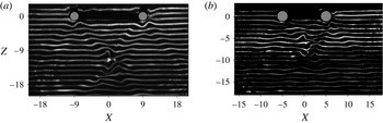
1 Introduction
In the oceans, the interaction of the tidal motion with the bottom topography is continuously generating internal waves (Bell Reference Bell1975; Vlasenko, Stashchuk & Hutter Reference Vlasenko, Stashchuk and Hutter2005; Garrett & Kunze Reference Garrett and Kunze2007). There is a reasonable agreement about the global rate of energy of 3.7 TW from lunar and solar tides, of which approximately 1 TW is converted into the baroclinic tide (Morozov Reference Morozov1995; Garrett & Kunze Reference Garrett and Kunze2007). The transfer of this energy into mixing is relevant to the general circulation in the oceans, and is therefore also of interest to climate modelling (Wunsch & Ferrari Reference Wunsch and Ferrari2004; Ferrari & Wunsch Reference Ferrari and Wunsch2008).
Over the past decades, the mechanism of internal wave generation has been studied in some detail for oscillating objects of various idealized geometries. Most well known are the classical flow visualizations of Mowbray & Rarity (Reference Mowbray and Rarity1967) of wave rays emitted by an oscillating cylinder in the shape of a St Andrews cross. Linear theory for two-dimensional internal waves generated by the oscillation of an elliptical cylinder of Hurley (Reference Hurley1997) and Hurley & Keady (Reference Hurley and Keady1997) was shown to be in good agreement with quantitative experimental results (see Sutherland et al. Reference Sutherland, Dalziel, Hughes and Linden1999, Reference Sutherland, Hughes, Dalziel and Linden2000; Sutherland & Linden Reference Sutherland and Linden2002; Ermanyuk Reference Ermanyuk2000; Ermanyuk & Gavrilov Reference Ermanyuk and Gavrilov2002). For ridges of Gaussian, exponential or witch-of-Agnesi shape Llewellyn Smith & Young (Reference Llewellyn Smith and Young2002) extended analytic estimates of Bell (Reference Bell1975) to compare internal tidal conversion rate, an approach that later was applied to the waves generated by a vertical barrier (Llewellyn Smith & Young Reference Llewellyn Smith and Young2003). The ridge- and plateau-type geometries of specific shape are shown to generate no propagating internal waves for certain frequencies and depths (Maas Reference Maas2011).
Three-dimensional effects of internal waves are particularly considered in King, Zhang & Swinney (Reference King, Zhang and Swinney2009). For a horizontally oscillating hemisphere they revealed the conical structure of wave beams and asymmetric bimodal structure. For moderate forcing, a flow perpendicular to the forcing direction was found, leading to a large-scale horizontal circulation. The internal wave pattern generated by a horizontally oscillating sphere was compared with the three-dimensional linear theory in Voisin, Ermanyuk & Flór (Reference Voisin, Ermanyuk and Flór2011). This theory included viscous effects and showed good agreement with experiments at low oscillation amplitude, and also allowed to better investigate the transition from bimodal to unimodal waves. At moderate oscillation amplitude, the propagative first and second harmonics were shown to have radically different horizontal patterns and are respectively of dipole and quadrupole type in the horizontal plane (Ermanyuk, Flór & Voisin Reference Ermanyuk, Flór and Voisin2011). More complex geometries have also been considered. Bühler & Muller (Reference Bühler and Muller2007) developed the linear theory for the oscillation of a ring with a subcritical Gaussian generatrix, and consider for the first time the effect of geometric focusing of wave energy into localized regions of high wave amplitude. Some examples on this effect of focusing were given. For a circular Gaussian hill and horseshoe topography also the mean flow localized in regions of wave dissipation have been considered (Grisouard & Bühler Reference Grisouard and Bühler2012).
As mentioned above, a main interest in internal wave dynamics is the conversion of wave energy into mixing and small-scale dissipation due to a rich variety of mechanisms including wave–wave and wave–current interactions, and overturning motions. Several scenarios have been considered for the energy concentration of internal waves in localized zones, of which we recall the most recurrent ones: (i) nearly critical reflection at continental slope (e.g. Dauxois & Young Reference Dauxois and Young1999; Gayen & Sarkar Reference Gayen and Sarkar2010), (ii) energy concentration at attractors (Maas et al. Reference Maas, Benielli, Sommeria and Lam1997; Echeverri et al. Reference Echeverri, Yokossi, Balmforth and Peacock2011; Scolan, Ermanyuk & Dauxois Reference Scolan, Ermanyuk and Dauxois2013; Guo & Holmes-Cerfon Reference Guo and Holmes-Cerfon2016), (iii) internal wave refraction at horizons of high density gradient (e.g. Mathur & Peacock Reference Mathur and Peacock2009), (iv) interaction of wave beams in two dimensions (Teoh, Ivey & Imberger Reference Teoh, Ivey and Imberger1997; Xing & Davies Reference Xing and Davies2011; Zhang & Swinney Reference Zhang and Swinney2014) and, as mentioned above, (v) geometric focusing by three-dimensional topography (Bühler & Muller Reference Bühler and Muller2007; Grisouard & Bühler Reference Grisouard and Bühler2012), recently also observed near canyons (Dale & Inall Reference Dale and Inall2015; Vlasenko et al. Reference Vlasenko, Stashchuk, Inall, Porter and Aleynik2016).
These latter studies (v) are novel compared to the various types of two-dimensional focusing because of the convergence of the internal wave rays. Similarly as light waves passing through a convex lens the wave rays converge to a focal point, adding a fundamentally new aspect to the internal wave dynamics. Conservation of energy flux through a surface which reduces with distance, implies a continuous increase of energy density along the rays towards the focal point and a decrease after passing through it.
Geometric focusing of internal wave energy has hardly been investigated experimentally. Wave focusing may occur near an oscillating hemisphere (see figure 3 in King et al. Reference King, Zhang and Swinney2009) and Gaussian mountain (see figure 3e in King, Zhang & Swinney Reference King, Zhang and Swinney2010), but was not discussed. The focusing effect increases with the radius and size of the oscillating object since more energy is transported to the focal zone, but in general its effect is negligible in small-scale laboratory experiments with small oscillating spherical objects and has therefore not been reported before. First experiments with a 60 cm diameter vertically oscillating torus revealed a strong vortical motion with wave overturning and local mixing in the focal zone (unpublished results, Flór 1997). In a similar experiment in a rotating fluid, inertial waves were shown to generate turbulence in the focal zone (Duran-Matute et al. Reference Duran-Matute, Flór, Godeferd and Jause-Labert2013). In the context of the tidal motion in the oceans, a horizontal oscillation is more appropriate. The horizontal oscillation direction also gives a direction to the overturning motions in the focal region, and therefore generates a mean flow that may be relevant to ocean applications (see Bühler Reference Bühler2009).
In the present paper we investigate the wave pattern generated by a horizontally oscillating torus, the criterion for the onset of wave breaking and observations of the nonlinear aspects of the wave generation in the focal region. We focus on the linear and weakly nonlinear regime, and consider the second harmonic generation and mean flow aspects in a separate contribution. The oscillating torus (or ring) generates ‘outward’ moving diverging waves and ‘inward’ converging waves. As is known from previous studies on the oscillation of three-dimensional objects of spherical geometry (see Flynn, Onu & Sutherland Reference Flynn, Onu and Sutherland2003; King et al. Reference King, Zhang and Swinney2009; Ermanyuk et al. Reference Ermanyuk, Flór and Voisin2011; Voisin et al. Reference Voisin, Ermanyuk and Flór2011), diverging waves gradually decrease in amplitude with distance due to the increasing cross-section of the wave cone and viscous dissipation. For the present flows under consideration, the diverging waves are indeed relatively weak. The converging waves, however, increase in amplitude with distance from the torus toward the focal regions, leading to wave amplification and breaking.
In the next section, § 2, theoretical considerations are presented on the focusing of internal waves. The description of the experimental installation and techniques is given in § 3 of the present paper. The results of experiments with internal waves are described in § 4, and the main results and possible oceanic applications are presented in § 5.
2 Theoretical considerations
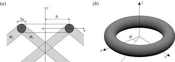
Geometry of the torus: in (a) view in vertical plane and (b) three-dimensional view defining the coordinate system.

We consider a torus of which the geometrical parameters are defined in figure 1. The torus is submerged into a uniformly stratified fluid with the buoyancy frequency
 $N=[(-g/\unicode[STIX]{x1D70C})\unicode[STIX]{x2202}\unicode[STIX]{x1D70C}/\unicode[STIX]{x2202}z]^{1/2}$
, where
 $\unicode[STIX]{x1D70C}(z)$
is the density distribution in
 $z$
-direction and
 $g$
is the gravitational acceleration. It has a circular generatrix with
 $a$
the radius of the tube (i.e. minor radius), and major radius
 $b$
the distance from the tube centre to the torus centre (see figure 1
a). A Cartesian coordinate system (see figure 1
b) is introduced, with the
 $z$
-axis pointing upwards. The origin of the coordinate system
 $O$
is taken at the mean position of the centre of the torus which undergoes rectilinear harmonic oscillations with frequency
 $\unicode[STIX]{x1D714}$
. The non-dimensional geometry can be characterized by the aspect ratio
 $\unicode[STIX]{x1D716}=b/a$
. We assume that the torus is slender, i.e.
 $\unicode[STIX]{x1D716}$
is large. The non-dimensional coordinates
 $X$
,
 $Y$
and
 $Z$
are introduced after normalization of
 $x$
,
 $y$
and
 $z$
with the radius of the generatrix,
 $a$
.
Let us consider first the vertical oscillations of the torus with amplitude
 $A$
, which is assumed to be small compared to
 $a$
so that the Keulegan–Carpenter number
 $Ke=A/a\ll 1$
. The Stokes number defined as
 $\unicode[STIX]{x1D6FD}=\unicode[STIX]{x1D714}a^{2}/\unicode[STIX]{x1D708}$
, with
 $\unicode[STIX]{x1D708}$
the kinematic viscosity, is assumed to be sufficiently large, i.e.
 $\unicode[STIX]{x1D6FD}\gg 1$
. In the experiments described below,
 $\unicode[STIX]{x1D6FD}=O(100)$
which guarantees a sufficiently small non-dimensional boundary layer thickness
 $\unicode[STIX]{x1D6FF}/a$
. To construct an approximate solution we use an approach similar to the strip theory in marine hydrodynamics (Newman Reference Newman1977a
,Reference Newman
b
).
Suppose that each radial cross-section of the torus oscillates vertically and generates internal wave beams described by (3.7) in Hurley & Keady (Reference Hurley and Keady1997). For brevity this equation is not reproduced here. Indeed, assumptions
 $Ke=A/a\ll 1$
and
 $\unicode[STIX]{x1D6FD}\gg 1$
are in agreement with Hurley & Keady (Reference Hurley and Keady1997). This linear solution plays a role of an ‘inner’ solution, which is approximately valid at each radial cross-section
 $\unicode[STIX]{x1D719}=\text{const.}$
, where
 $\unicode[STIX]{x1D719}$
is an azimuthal angle in the cylindrical coordinate system
 $(r,z,\unicode[STIX]{x1D719})$
, with
 $r=(x^{2}+y^{2})^{1/2}$
. For vertical oscillations the problem is axisymmetric and all cross-sections
 $\unicode[STIX]{x1D719}=\text{const.}$
are equivalent. Without loss of generality we consider oscillations in the plane
 $xOz$
(see figure 1). The streamfunction for a single cylinder,
 $$\begin{eqnarray}\displaystyle \unicode[STIX]{x1D713}_{HK}^{1}(x,z,t)=\unicode[STIX]{x1D6F9}_{HK}^{1}(x,z)\exp (\text{i}\unicode[STIX]{x1D714}t), & & \displaystyle\end{eqnarray}$$
is constructed as a sum of four streamfunctions describing the four beams of the St. Andrew cross wave pattern (see Sutherland et al. Reference Sutherland, Dalziel, Hughes and Linden1999)
 $$\begin{eqnarray}\unicode[STIX]{x1D6F9}_{HK}^{1}(x,z)=\unicode[STIX]{x1D6F9}_{l}^{+}+\unicode[STIX]{x1D6F9}_{r}^{+}+\unicode[STIX]{x1D6F9}_{l}^{-}+\unicode[STIX]{x1D6F9}_{r}^{-},\end{eqnarray}$$
where the superscripts
 $+$
and
 $-$
refer, respectively, to the upper and lower half-planes, whereas the subscripts
 $l$
and
 $r$
refer, respectively, to the beams propagating to the left and the right.
For the second cylinder the solution
 $\unicode[STIX]{x1D6F9}_{HK}^{2}(x,z)$
is analogous. Assuming that
 $b/a$
is sufficiently large, the solution for the system of two cylinders can be written as
 $$\begin{eqnarray}\unicode[STIX]{x1D6F9}_{HK}(x,z)=\unicode[STIX]{x1D6F9}_{HK}^{1}(x,z)+\unicode[STIX]{x1D6F9}_{HK}^{2}(x,z),\end{eqnarray}$$
where the appropriate choice of signs and phases in (2.2) assure that both cylinders oscillate vertically and in phase. The instantaneous vertical displacement of fluid particles due to the oscillation of two cylinders is then evaluated as
 $$\begin{eqnarray}\unicode[STIX]{x1D701}_{HK}^{t}(x,z,t)=(\text{i}/\unicode[STIX]{x1D714})\exp (\text{i}\unicode[STIX]{x1D714}t)\frac{\unicode[STIX]{x2202}}{\unicode[STIX]{x2202}x}\unicode[STIX]{x1D6F9}_{HK}(x,z).\end{eqnarray}$$
The corresponding distribution of wave amplitudes is denoted as
 $\unicode[STIX]{x1D701}_{HK}(x,z)$
.
Further, we introduce the geometric correction factor for convergence (divergence) of the wave field. Let us consider a point
 $C$
with coordinates (
 $x_{C},z_{C}$
) in the two-dimensional wave field generated by a system of two cylinders. The density of the energy flux at point
 $C$
is proportional to the wave amplitude squared
 $(\unicode[STIX]{x1D701}_{HK}(x_{C},z_{C}))^{2}$
. Since the torus is slender, we can equate the energy fluxes due to internal waves emitted by vertical oscillations of a torus of mean radius
 $b$
and small radius
 $a$
, and due to a system of two cylinders (see figure 1) of radius
 $a$
and length
 $\unicode[STIX]{x03C0}b$
. We obtain then
 $$\begin{eqnarray}\displaystyle (\unicode[STIX]{x1D701}(r_{C},z_{C}))^{2}\unicode[STIX]{x03C0}r_{C}=(\unicode[STIX]{x1D701}_{HK}(x_{C},z_{C}))^{2}\unicode[STIX]{x03C0}b, & & \displaystyle\end{eqnarray}$$
where
 $r_{C}=x_{C}$
at
 $\unicode[STIX]{x1D719}=0$
. Finally, we obtain in non-dimensional cylindrical coordinates
 $$\begin{eqnarray}\unicode[STIX]{x1D701}(R,Z)=(R/\unicode[STIX]{x1D716})^{-1/2}\unicode[STIX]{x1D701}_{HK}(R,Z),\end{eqnarray}$$
where
 $R=r/a$
. The term
 $(R/\unicode[STIX]{x1D716})^{-1/2}$
assures a proper decay of the wave amplitude at infinity.
Let us note that in the case of vertical oscillations of two cylinders the wave amplitude
 $\unicode[STIX]{x1D701}_{HK}(x,z)$
is symmetric with the respect to the vertical axis
 $x=0$
and non-zero at
 $x=0$
. Therefore the approximate solution predicts a divergence of wave amplitudes of the form of
 $X^{-1/2}$
in the focal region at
 $X\rightarrow 0$
. This result shows that near-field interactions should be taken into account in this zone in order to develop a more advanced linear theory. Also, in realistic situations, one can expect strong spatially localized nonlinear effects in the form of vertical jets. Such effects have been indeed observed for inertial waves in Duran-Matute et al. (Reference Duran-Matute, Flór, Godeferd and Jause-Labert2013) and have been shown to create a localized turbulence zone due to a cascade of instability events.
Now, let us adapt the same approach in the spirit of strip theory (Newman Reference Newman1977a
,Reference Newman
b
) to a slender torus undergoing horizontal oscillations with amplitude
 $A$
along the
 $x$
-axis. The local forcing is then taken as a projection of horizontal oscillations on the radial coordinate of the form
 $A\cos \unicode[STIX]{x1D719}$
. Obviously, equations (2.2)–(2.4) remain valid in the case of horizontal oscillations of a system of two cylinders, with the important difference that the signs and phases of motions in wave beams should now be chosen such that the wave amplitude
 $\unicode[STIX]{x1D701}_{HK}(x,z)=0$
at
 $x=0$
and the instantaneous wave profiles are antisymmetric with respect to the vertical axis
 $x=0$
. The geometric conversion introduced in (2.6) remains valid but now, owing to azimuthal modulation of the wave field, (2.6) transforms into
 $$\begin{eqnarray}\displaystyle \unicode[STIX]{x1D701}(R,Z,\unicode[STIX]{x1D703})=(R/\unicode[STIX]{x1D716})^{-1/2}\unicode[STIX]{x1D701}_{HK}(R,Z)|\cos \,\unicode[STIX]{x1D703}|. & & \displaystyle\end{eqnarray}$$
For horizontal oscillations,
 $\unicode[STIX]{x1D701}_{HK}(R,Z)$
is proportional to
 $R$
at a fixed
 $Z$
in a small vicinity of
 $R=0$
, and therefore
 $\unicode[STIX]{x1D701}(R,Z,\unicode[STIX]{x1D703})$
is proportional to
 $R^{1/2}$
as
 $R$
tends to 0. Thus, the wave amplitude remains limited but the wave slope tends to the vertical. This qualitatively indicates a possibility of overturning in the focal region, which is a qualitatively different behaviour compared to the case of vertical oscillations.
To characterize the forcing of internal waves, the Keulegan–Carpenter number
 $Ke=A/a$
is often used (see e.g. Ermanyuk et al.
Reference Ermanyuk, Flór and Voisin2011; Voisin et al.
Reference Voisin, Ermanyuk and Flór2011). Although this number characterizes the nonlinearity close to the torus, it does not take into account the geometric effect of focusing at larger distances from the torus. Supposing that in the focal zone the wave motion can be confined to a zone with radius
 $a$
, the amplitude may increase to
 $\unicode[STIX]{x1D701}_{corr}=\unicode[STIX]{x1D701}_{HK}(b/a)^{1/2}=\unicode[STIX]{x1D701}_{HK}\unicode[STIX]{x1D716}^{1/2}$
i.e. with a factor
 $\unicode[STIX]{x1D716}^{1/2}$
due to focusing. The same correction factor has been introduced earlier in Bühler & Muller (Reference Bühler and Muller2007). Note that the above-described theory neglects the near-field wave interactions in the focal region. Also, the viscous damping in the above solution is adapted from Hurley & Keady (Reference Hurley and Keady1997), and therefore neglects additional shear close to the focal region. Therefore it is expected to provide a quantitative estimate with a reasonable accuracy only in the vicinity of the torus. The effects of finite values of
 $Ke$
,
 $\unicode[STIX]{x1D6FD}$
and
 $\unicode[STIX]{x1D716}$
in experiments are discussed below.
When oscillating an obstacle with frequency
 $\unicode[STIX]{x1D714}$
, in addition to the fundamental first harmonic wave oscillating at frequency
 $\unicode[STIX]{x1D714}$
, the dispersion relation admits wave radiation for higher harmonics with frequencies
 $n\unicode[STIX]{x1D714}$
, where
 $n=2,3,\ldots ,$
were
 $\unicode[STIX]{x1D714}n<N$
(see Mowbray & Rarity Reference Mowbray and Rarity1967). In contrast, for
 $\unicode[STIX]{x1D714}>N/2$
all higher harmonics are evanescent. In the experiments described below the value of
 $\unicode[STIX]{x1D6FA}=\unicode[STIX]{x1D714}/N>0.5$
so that the higher harmonics are evanescent and the effect due to focusing of the first harmonic waves emitted by the torus can be studied in isolation.
3 Experimental set-up and measurement procedure
3.1 Experimental set-up
To measure the evolution of wave amplitudes and slopes with distance from the ring we use the laser induced fluorescein (LIF) technique (for details see Ermanyuk et al. Reference Ermanyuk, Flór and Voisin2011; Voisin et al. Reference Voisin, Ermanyuk and Flór2011).
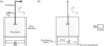
Sketch of the experimental set-up: (a) front view and (b) side view, with the light grey lines the fluorescein dye planes and the laser plane shown in dark grey.
 $(X,Y,Z)=(x,y,z)/a$
are the non-dimensional coordinates. The torus oscillates in the
 $X$
-direction (plane of view),
 $Z$
is in the vertical direction. The mobility of the laser plane in the
 $Y$
-direction allows for the measurement of successive planes, and the reconstitution of the horizontal wave field.

This technique is based on the accurate tracking of distortions of isodensity surfaces (fluorescent dye planes), and allows us to measure the amplitude of the vertical velocity with a very high precision. Since dye tracers are followed in time the recording is of Lagrangian type, in contrast with Eulerian-type techniques (particle image velocimetry or synthetic schlieren) usually employed in experimental studies on waves. For waves of small amplitude the two types of measurements yield essentially the same results. As the wave amplitude increases, Lagrangian measurements allow us to study the evolution of wave profiles toward overturning via direct measurement of wave slopes. Complementary particle image velocimetry (PIV) measurements provided information about profiles of horizontal velocity and its distribution over a horizontal plane.
Two tori have been used in the present experiments, a ‘thin ring’ with
 $a=1.5~\text{cm}$
and
 $b=13.5~\text{cm}$
, and a ‘thick ring’ with
 $a=2~\text{cm}$
and
 $b=10~\text{cm}$
. The aspect ratio
 $\unicode[STIX]{x1D716}=b/a$
is respectively equal to 9 for the ‘thin’, and 5 for the ‘thick’ one. At the experimental value of frequency
 $\unicode[STIX]{x1D714}=0.65~\text{rad}~\text{s}^{-1}$
the Stokes numbers are
 $\unicode[STIX]{x1D6FD}=150$
and 260 respectively for the thin and the thick torus.
The experiments are conducted in a Plexiglas
 $100~\text{cm}$
cubic tank filled to a working depth of 90 cm with a linearly salt-stratified fluid using the conventional double-bucket technique (see figure 2). The stratification profile is calculated from the density of fluid samples taken at different heights in the fluid and measured with an Anton Paar density meter. The values of the buoyancy frequency
 $N$
are listed in table 1.
Internal waves are generated by a horizontally oscillating Plexiglas torus that is painted black to avoid laser light reflections. It is attached to the end of a pendulum of length
 $l=180~\text{cm}$
, and the oscillations of the pendulum at frequency
 $\unicode[STIX]{x1D714}$
are driven by a crank mechanism. The oscillation amplitude,
 $A$
, of the torus is small compared to the length of the pendulum, and the motion is therefore in good approximation horizontal and sinusoidal. The two side walls perpendicular to the direction of the oscillation of the cylinder are covered with a mesh of 5 cm thickness to avoid wave reflections. In some cases also the bottom and the back wall were covered with wave absorbers, but no difference in results could be noticed. After 10 oscillation periods the wave pattern reaches the steady state in the region of interest. Measurements are taken after
 $20$
oscillations, which is the typical duration used to exclude the effects of internal wave transients (see Voisin Reference Voisin2003; Ermanyuk & Gavrilov Reference Ermanyuk and Gavrilov2005, Reference Ermanyuk and Gavrilov2008; Voisin et al.
Reference Voisin, Ermanyuk and Flór2011).
For the method of fluorescein dye planes (first employed in Hopfinger et al. Reference Hopfinger, Flór, Chomaz and Bonneton1991 and Flór, Ungarish & Bush Reference Flór, Ungarish and Bush2002), a set of equidistant dye planes is generated by slowly displacing a rake of horizontally spanned cotton threads through the fluid. These cotton threads are soaked in a concentrated fluorescein solution and dried before the experiment. The dye planes are illuminated with a vertical laser sheet parallel to the direction of oscillations. The data processing is performed with a version of cross-correlation technique described in Ermanyuk et al. (Reference Ermanyuk, Flór and Voisin2011) and Voisin et al. (Reference Voisin, Ermanyuk and Flór2011), from which the vertical displacements of the dye lines are determined with the accuracy of approximately 0.05 pixel. The laser sheet is perpendicular to the dye planes and shows therefore dye lines on the recordings (see figure 9).
Experimental parameters, with
 $\unicode[STIX]{x1D716}=b/a$
the torus aspect ratio,
 $Ke=A/a$
the Keulegan–Carpenter number and
 $\unicode[STIX]{x1D6FA}=\unicode[STIX]{x1D714}/N$
, where
 $A$
and
 $\unicode[STIX]{x1D714}$
are respectively the oscillation amplitude and frequency and
 $Z_{focal}$
corresponds to the geometrical point of intersection of the wave rays. The buoyancy frequency,
 $N$
, is represented in dimensional values.

Prior to the onset of the oscillations, the horizontal dye planes are scanned by a laser sheet in the otherwise quiescent fluid to obtain the reference state
 $\unicode[STIX]{x1D701}_{0}$
for each dye plane. The vertical displacement of these dyelines,
 $\unicode[STIX]{x1D701}^{\prime }$
, is measured at a certain position in time with respect to the reference state
 $\unicode[STIX]{x1D701}_{0}$
, i.e.
 $\unicode[STIX]{x1D701}^{\prime }(x,t)=\unicode[STIX]{x1D701}^{\prime }-\unicode[STIX]{x1D701}_{0}^{\prime }$
(the prime is to note that this value does not necessarily correspond to a particle displacement). The local slopes of wave profiles in plane
 $XZ$
are measured as
 $s(t)=\arctan (\text{d}\unicode[STIX]{x1D701}(t)/\text{d}x)$
. In practice the slope at position
 $(X,Z)$
is evaluated as
 $$\begin{eqnarray}s(t)=\arctan (\unicode[STIX]{x0394}\unicode[STIX]{x1D701}(t)/\unicode[STIX]{x0394}x),\end{eqnarray}$$
where
 $\unicode[STIX]{x0394}x$
should be sufficiently large compared to the accuracy of measurement of vertical displacements
 $\unicode[STIX]{x1D701}(t)$
and sufficiently small compared to the radius of the generatrix
 $a$
to resolve the details of wave profiles. The wave slope represents a sensitive and physically important measure of the baroclinic torque of the wave, caused by the shear. This slope is related to the Richardson number and is therefore an indication for overturning, as is discussed further in § 4.4. As described in Ermanyuk et al. (Reference Ermanyuk, Flór and Voisin2011) and Voisin et al. (Reference Voisin, Ermanyuk and Flór2011), the vertical displacements are evaluated as the average values over vertical stripes of width of several pixels, which defines the horizontal spatial resolution of the experimental data. In the present experiments
 $\unicode[STIX]{x0394}x$
is taken equal to the horizontal spatial resolution, with
 $\unicode[STIX]{x0394}x=5$
(
 ${\approx}0.253$
cm) and 8 pixels (
 ${\approx}0.339$
cm) for respectively the ‘thin’ and the ‘thick’ torus.
To reconstruct a quasi-three-dimensional distribution of the wave amplitudes (note that the velocity in
 $y$
-direction is not measured), a series of images was acquired for different positions in
 $y$
-direction. Therefore, the mirror reflecting the laser light (see figure 2) was moved by a computer-controlled step motor with a prescribed increment
 $\unicode[STIX]{x0394}y=0.8~\text{cm}$
. At each position the mirror remained fixed during one period of oscillation. This allowed to acquire time series suitable for subsequent Fourier analysis and evaluation of amplitudes of harmonic components.
For the PIV measurement the algorithm of Fincham & Delerce (Reference Fincham and Delerce2000) was used, and the optimum particle size and seeding density of Westerweel (Reference Westerweel1997) were followed. The fluid was seeded with Orgasol®
 $30~\unicode[STIX]{x03BC}\text{m}$
particles of density
 $\unicode[STIX]{x1D70C}=1.2~\text{kg}~\text{m}^{-3}$
, illuminated with a vertical and horizontal laser sheet. The particle displacement was obtained using the UVMAT/CIVx software package developed at LEGI (http://www.legi.cnrs.fr/web/spip.php?article763). Successive images are taken with a time increment of
 $\unicode[STIX]{x0394}t=t_{i+1}-t_{i}=0.5~\text{s}$
, which is kept constant in all experiments.
3.2 Data analysis and parameters
Time series of vertical displacements
 $\unicode[STIX]{x1D701}(t_{i})$
are analysed using three different methods. With the first method, the amplitudes of the
 $n$
th harmonic components of the signal
 $\unicode[STIX]{x1D701}_{n}$
and
 $S_{n}$
are determined via Fourier filtering of time series. Similar analysis has been used in Ermanyuk et al. (Reference Ermanyuk, Flór and Voisin2011) and Voisin et al. (Reference Voisin, Ermanyuk and Flór2011). This type of data processing is particularly useful for linear or weakly nonlinear processes when the first few harmonics are dominant and can be clearly identified. With the second method, the amplitudes
 $\unicode[STIX]{x1D701}_{rms}$
and
 $S_{rms}$
are evaluated as the period-averaged root mean square of the corresponding time series multiplied by
 $2^{1/2}$
(Sutherland & Linden Reference Sutherland and Linden2002). In principle, this quantity takes into account the contribution of all harmonics in the signal. However, owing to the period averaging procedure the root-mean-square value cannot precisely capture the extreme values of wave amplitude and wave slope, which may instantly occur at a particular phase of oscillation. Of special interest are the extreme slopes which can trigger incipient overturning in the case wave crests become steep. Therefore, a third method of data processing was introduced. Time series
 $\unicode[STIX]{x1D701}(t_{i})$
and
 $s(t_{i})$
measured at each point were sorted to find the maximum values of
 $\unicode[STIX]{x1D701}_{max}=\max |\unicode[STIX]{x1D701}(t_{i})|$
and
 $S_{max}=\max |s(t_{i})|$
.
Thus with these three methods, next to the values
 $\unicode[STIX]{x1D701}_{n}$
,
 $\unicode[STIX]{x1D701}_{rms}$
and
 $\unicode[STIX]{x1D701}_{max}$
, the slopes
 $S_{n}$
,
 $S_{rms}$
and
 $S_{max}$
were measured in degrees allowing to explicitly study the transition of the wave system to overturning. The wave amplitudes are normalized generally with the oscillation amplitude,
 $A$
, or in case only the focal region is of interest, the generatrix of the torus,
 $a$
. The governing parameters of experimental runs performed in this study are presented in table 1.
4 Results and discussion
4.1 Wave pattern in
 $XZ$
-plane

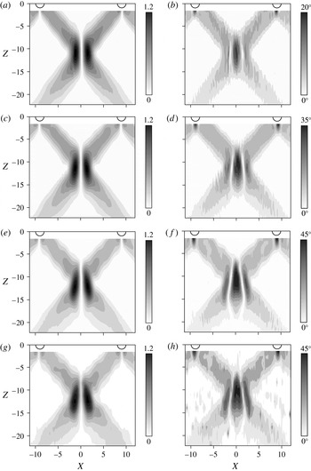
Contour plots of the wave amplitude
 $\unicode[STIX]{x1D701}_{1}/A$
(a,c,e,g) and wave slope
 $S_{1}$
(b,d,f,h) in the
 $XZ$
-plane, with (a,b)
 $Ke=0.19$
; (c,d)
 $0.41$
and (e,f)
 $0.65$
. (g,h) Contour plots for
 $\unicode[STIX]{x1D701}_{max}/A$
and
 $S_{max}$
for
 $Ke=0.65$
. Exp A, with torus aspect ratio
 $\unicode[STIX]{x1D716}=9$
. Data are obtained from LIF measurements.

Figures 3(a)–3(f) show the typical evolution of the first harmonic wave patterns for different oscillation amplitude, represented by the Keulegan–Carpenter number
 $Ke$
, in terms of contours of wave amplitude
 $\unicode[STIX]{x1D701}_{1}/A$
and contours of wave slope
 $S_{1}$
. For comparison figures 3(g) and 3(h) represent the unfiltered wave fields in terms of
 $\unicode[STIX]{x1D701}_{max}/A$
and
 $S_{max}$
. A higher level of noise is observed for these non-filtered max-type quantities. Figures 3(e)–3(h) show a high resemblance indicating that at moderate oscillation amplitude, the dominant contribution to the wave field is represented by the first harmonic wave obtained after Fourier filtering, as can be expected since higher harmonics are evanescent for this forcing.
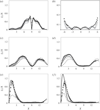
Normalized wave amplitude
 $\unicode[STIX]{x1D701}_{1}/A$
for Exp A at different heights
 $Z$
below the centre of the torus, with (a)
 $Z=-1.84$
, (b)
 $Z=-1.84$
zoomed in including negative values of
 $X$
(the centre line of the torus is at
 $X=0$
); (c)
 $Z=-4.48$
; (d)
 $-7.17$
; (e)
 $-9.84$
and (f)
 $-12.51$
. The focal zone is located at
 $Z=-11.2$
. The dashed and solid lines represent, respectively, the theoretical profile (2.6) obtained for two oscillating cylinders, and the profile corrected for convergence; black, grey and light grey dots correspond respectively to
 $Ke=0.19,0.41$
and
 $0.65$
. Data are obtained from LIF experiments.

Wave amplitudes close to the torus are roughly two times smaller than the wave amplitudes in the focal region, but the wave slopes close to the torus and in the focal region are comparable. The onset of overturning occurs therefore not only in the focal region but also near to the torus. It should be noted that this latter overturning is rather due to the steep topography, an effect that would most likely be absent for a Gaussian-shaped torus. At low
 $Ke$
the amplified wave amplitude in the focal region forms then two symmetric ellipses due to the antisymmetry of the instantaneous wave profiles with respect to
 $YZ$
plane, where the wave amplitude is zero. As
 $Ke$
increases, these regions of maximum amplitude slightly shift into the
 $Z$
-direction away from the torus. The nonlinear evolution of the wave field is well visible in terms of wave slopes. At low
 $Ke$
the focal region (figure 3
b) is nearly elliptic. As
 $Ke$
increases, the focal region takes a spearhead-like shape (figure 3
f,h), indicating the higher shear in the outer region of the focal region and incipient overturning. As a consequence, the waves are hindered by nonlinear effects in the focal region.
Note also that the waves in the focal zone have a unimodal structure, i.e. there is a single wave beam due to the presence of viscosity in contrast to the bimodal structure often observed very near to oscillating objects (for a discussion see e.g. Voisin et al.
Reference Voisin, Ermanyuk and Flór2011). Though the general flow evolution was very similar to that of the thick torus (
 $\unicode[STIX]{x1D716}=5$
), its larger generatrix
 $a$
implied a larger Stokes number, (260 instead of 150) causing a rather bimodal wave structure near the torus which turned into a single beam near the focal region. In the case of very large tori, however, one may expect a multi focal region because of the bimodal wave structure. In view of the range of accessible Stokes numbers, this was not observed in the present experiments.
4.2 Comparison of measurements with linear theory
Figure 4 shows the wave amplitude across the wave beam measured in plane
 $XZ$
at different distances
 $Z$
from the centre of the torus. The experimental distributions of the scaled amplitude,
 $\unicode[STIX]{x1D701}_{1}(X)/A$
for the torus with
 $\unicode[STIX]{x1D716}=9$
are presented for a range of
 $|Z|$
values up to the middle of the focal zone. Good agreement with the theory described in § 2 is observed at low values of
 $Ke$
, and close to the torus. Thus, a simple geometric correction is fully sufficient for quantitative description of the main effects due to convergence (divergence) of waves in the vicinity of a curved elongated body. Thereby it provides a consistent framework for quantitative interpretation of the experimental results almost everywhere in the wave field, except the focal region.
For the focal region, the theory shows that focusing amplifies the wave amplitude to a factor 3, in qualitative agreement with the correction factor
 $\unicode[STIX]{x1D716}^{1/2}$
introduced in Bühler & Muller (Reference Bühler and Muller2007). This can be observed in figure 4(f) (
 $|Z|=12.51$
) from the comparison of the calculated wave amplitudes for the torus (solid line) and the reference case of the two parallel cylinders of infinite length (dash line). The experimentally measured wave amplitudes in the focal zone are significantly lower (approximately by 30 %) than the theoretical estimate. Indeed the theory presented in § 2 neglects the near-field interactions between the wave components in the focal zone, leading to unrealistic infinite wave slopes at the vertical axis
 $Z$
.
The experimental data presented in figure 4 provide qualitative information on the nonlinear trends in the wave amplitude as function of the oscillation amplitude
 $Ke$
. With increasing
 $Ke$
, the normalized wave amplitude of the first harmonic,
 $\unicode[STIX]{x1D701}_{1}/A$
typically decreases almost everywhere in the wave field except the focal region: the amplitude profiles marked by light grey and grey symbols are consistently lower than the profiles marked by black symbols. This trend is in agreement with the nonlinear trends observed for the two- (Zhang, King & Swinney Reference Zhang, King and Swinney2007) and three-dimensional (Ermanyuk et al.
Reference Ermanyuk, Flór and Voisin2011; Voisin et al.
Reference Voisin, Ermanyuk and Flór2011) cases. The opposite trend is seen in figure 4(f) in the focal region at
 $|Z|=12.51$
where higher normalized wave amplitudes
 $\unicode[STIX]{x1D701}_{1}/A$
correspond to higher
 $Ke$
. Thus, a linear extrapolation of the low-amplitude experimental data to a high-amplitude case should be done with care: it tends to underestimate the wave amplitudes in localized zones of the focal region and to overestimate the wave amplitudes in all other regions of the wave field. Interestingly, in the middle of the focal region, located at approximately
 $|Z|=11.2$
, the linear scenario applies in a remarkably wide range of
 $A$
as discussed below in § 4.4.
It is worth making a special remark concerning the data presented in figure 4(b). The low-amplitude standing wave pattern seen close to the centre of the torus can hardly be interpreted within a linear approach. The whole inner region delimited by the conical wave beams emitted by the torus seems to undergo a weak resonant motion. Its amplitude is typically an order of magnitude smaller than the amplitude of the main wave beams but at high oscillation amplitude
 $A$
it is high enough to deform the straight wave beams (compare the form of isolines of wave amplitudes in the first column of figure 3 at low and high amplitudes). The mechanism providing the energy flux to this motion is unclear and will be considered elsewhere.
4.3 Wave pattern in
$XY$
-plane

To study the azimuthal distribution of the wave amplitude, the wave fields in the
 $XY$
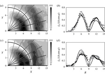
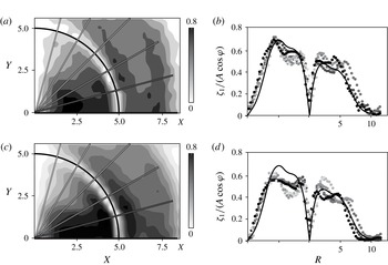
plane were reconstructed from series of images taken particularly in experiments Exp C and Exp D of table 1. Figures 5 and 6 show the contours of wave amplitudes and the normalized radial distributions of the vertical velocity amplitude of the first harmonic wave,
 $\unicode[STIX]{x1D701}_{1}(R)/(A\cos \unicode[STIX]{x1D719})$
close to the torus, with
 $\unicode[STIX]{x1D719}$
the angle with respect to the plane of symmetry. For this scaling, the data are found to collapse reasonably well on a more or less common curve, for both tori (see figures 5
b, 6
b). Also we note that the agreement with the linear theory presented in § 2 is within an error of approximately 10 % for both cases. For the thick torus (see figure 6
b) the shape of the wave envelope is slightly different due to its bimodal character. Also, here the theoretical prediction is still quite reasonable (note that the original theory of Hurley & Keady (Reference Hurley and Keady1997), used in § 2 takes bimodality and related viscous effects into account). For larger oscillation amplitudes (see figures 5
d, 6
d), the theoretical prediction is systematically higher than the measured values due to nonlinear effects. With increasing azimuthal angle,
 $\unicode[STIX]{x1D719}$
, the wave amplitude decreases, and therefore also the energy radiated by the torus. The departure of the observed profiles from the theoretical curve at
 $\unicode[STIX]{x1D719}$
tending to
 $90^{\circ }$
arises partially due to higher noise-to-signal ratio for these waves, and partially due to the fully three-dimensional nature of the flow. For azimuthal angles close to
 $90^{\circ }$
the cosine variation of wave amplitudes with the azimuthal angle is therefore no longer valid, especially for a thick torus.
Contours of the normalized wave amplitude
 $\unicode[STIX]{x1D701}_{1}/A$
(a,c) and the corresponding radial distributions
 $\unicode[STIX]{x1D701}_{1}(R)/(A\cos \unicode[STIX]{x1D711})$
(b,d) close to the torus for (a,b)
 $Ke=0.17$
and (c,d)
 $Ke=0.63$
, where
 $R=r/a$
is the non-dimensional radial coordinate. The black lines in (b) and (d) corresponds to (2.6). Exp C in table 1 (
 $Z=-3.6$
,
 $\unicode[STIX]{x1D716}=9$
). Data are obtained from LIF measurements.

As in figure 5 for the thick torus, with (a,b)
 $Ke=0.13$
and (c,d)
 $Ke=0.29$
, where
 $R=r/a$
is the non-dimensional radial coordinate. The black line corresponds to
 $\unicode[STIX]{x1D701}_{corr}$
. Exp D in table 1 (
 $Z=-3.0$
,
 $\unicode[STIX]{x1D716}=5$
). Data are obtained from LIF experiments.

4.4 Nonlinear effects: maximum wave amplitude and overturning
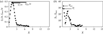
LIF measurements of wave amplitude (a) and wave slope (b) in the central plane according to the definitions given in § 3.2. Open circles indicate the first harmonic filtered values (
 $\unicode[STIX]{x1D701}_{1}/a$
,
 $S_{1}$
) and filled circles the unfiltered max-type estimate (
 $\unicode[STIX]{x1D701}_{max}/a$
,
 $S_{max}$
). The two represented levels are the focal zone at
 $Z=-12.51$
for
 $0<X<6$
(open and filled circles). The symbol
 $\ast$
refers to the extrema plotted in figure 8. Exp A:
 $Ke=0.41$
and
 $\unicode[STIX]{x1D716}=9$
.

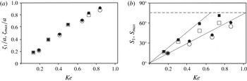
Maximum wave amplitude (a) and maximum wave slope (b) against
 $Ke$
. Filled and open symbols are as in figure 7 with circles for the thin torus with
 $\unicode[STIX]{x1D716}=9$
(at
 $Z=-12.51$
), and squares for the thick torus with
 $\unicode[STIX]{x1D716}=5$
(at
 $Z=-7$
). The dashed line at
 $\unicode[STIX]{x1D703}=75^{\circ }$
indicates the slope for which overturning is observed.


The variation of the maximum wave amplitude and maximum slope (measured as in figure 7
a,b) with the Keulegan–Carpenter number
 $Ke$
, are presented in respectively figures 8(a) and 8(b) for both tori. The overall good agreement between
 $\unicode[STIX]{x1D701}_{max}^{\ast }/a$
and
 $\unicode[STIX]{x1D701}_{1}^{\ast }/a$
confirms once again the expected dominance of the first harmonic wave for this forcing frequency (
 $\unicode[STIX]{x1D714}/N>0.5$
). For larger
 $Ke$
the increasing wave steepness and the increasing difference between
 $S_{max}^{\ast }$
and
 $S_{1}^{\ast }$
(see figure 8
b) suggest the presence of nonlinear effects. Incipient overturning is observed at
 $Ke=0.81$
and
 $Ke=1.1$
for tori with
 $\unicode[STIX]{x1D716}=5$
and
 $\unicode[STIX]{x1D716}=9$
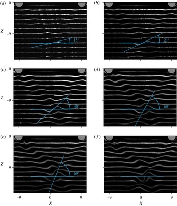
, respectively. From the dye images shown in figure 9, we indeed recognize well-developed overturning regions in the wave pattern. As expected, these regions are located close to the surface of the torus and in the focal region, corresponding to the zones of high local slopes which can be identified in figure 3.
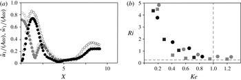
PIV measurements show (see figure 10 a) that in the focal region, the horizontal velocity of the first harmonic wave in the direction of oscillation is of the same magnitude as the vertical velocity. With the PIV data in the focal region, the horizontal shear and thus the local Richardson number in the wave can be calculated as
 $$\begin{eqnarray}\displaystyle Ri=\frac{N^{2}}{(\unicode[STIX]{x2202}\hat{u} _{1}/\unicode[STIX]{x2202}z)^{2}}, & & \displaystyle\end{eqnarray}$$
where the stratification
 $N$
is measured at the start of the experiment; the vertical gradient in velocity is measured from the PIV velocity data over a typical grid distance of
 $\unicode[STIX]{x0394}z=4~\text{pixels}$
(
 ${\approx}0.3~\text{cm}$
). The values of the this
 $Ri$
-number are displayed in grey in figure 10(b). Asymptotically a value of
 $Ri\approx 0.25$
is reached when
 $Ke$
approaches a value between
 $0.8$
and
 $1$
for different aspect ratio tori, corresponding for overturning in stratified shear flows (see Miles Reference Miles1961).
The Miles criterion is developed for a flow with vorticity due to the presence of a shear flow, and no baroclinic vorticity in its basic state. For the critical value of
 $Ri=0.25$
, vorticity of the shear flow is accumulated by the Kelvin–Helmholtz instability until breaking occurs. In the present experiments there is no shear flow, and the instability is not of the Kelvin–Helmholtz type. However, the amplitude of the waves is here represented by baroclinic vorticity. This amplitude (or baroclinic vorticity) is continuously increased due to focusing of wave energy, until the critical value is reached and breaking occurs. Though the sources of vorticity and mechanism for overturning are essentially different, the present results suggest that the criterion and, as shown below, the critical value are the same.
The LIF method allowed to precisely measure the wave slope of the wave for the different aspect ratio tori. Observations of visualizations showed a nearly linear dependence for
 $Ke<0.4$
with the waves remaining linear and passing almost without modification through the focal region. Small changes with respect to the linear regime were found to occur for
 $Ke$
around
 $0.6$
, whereas for approximately
 $Ke>0.8$
the onset of wave breaking is observed and waves are hindered to pass through the focal region. From this wave steepness one can derive directly the local wave Richardson number which can be defined as the ratio between the buoyancy frequency
 $N^{2}$
, and the
 $y$
-component of the baroclinic vorticity of the wave. This yields in the Boussinesq approximation,
 $$\begin{eqnarray}Ri_{wave}=N^{2}\left(\frac{\unicode[STIX]{x1D735}p\times \unicode[STIX]{x1D735}\unicode[STIX]{x1D70C}}{\unicode[STIX]{x1D70C}^{2}}\right)_{y}^{-1}\approx \frac{N^{2}}{-g\unicode[STIX]{x1D70C}\displaystyle \frac{\unicode[STIX]{x2202}\unicode[STIX]{x1D70C}}{\unicode[STIX]{x2202}x}}=\left.\frac{\unicode[STIX]{x0394}x}{\unicode[STIX]{x0394}z}\right|_{\unicode[STIX]{x1D70C}}=\frac{1}{\tan S},\end{eqnarray}$$
where the index
 $y$
indicates the
 $y$
component of the baroclinic vorticity vector. In figure 10(b) the wave Richardson number is displayed as a function of
 $Ke$
. Even though it is derived in a different manner, it shows also that wave breaking is reached when
 $Ri_{wave}\approx 0.25$
at
 $Ke\approx 0.8$
in coherence with the observations and the PIV measurements and shear instability. This local Richardson number indicates the maximum slope which an isopycnal plane may have before it becomes unstable and overturns. This overturning corresponds to a wave slope of
 $\unicode[STIX]{x1D703}\approx 75^{\circ }$
(see figure 8
b), the wave slope being measured over a horizontal length scale
 $\unicode[STIX]{x1D6FF}x$
(see § 3.1) near
 $X=0$
(see figure 11).
PIV measurement results with (a) horizontal and vertical velocity amplitude (respectively grey dots and black dots) along the
 $X$
-axis in the focal zone at
 $Z=-4.7$
for
 $\unicode[STIX]{x1D716}=5$
, with
 $Ke=0.19$
(filled dots) and
 $Ke=0.6$
(open dots); (b) Richardson numbers
 $Ri$
from PIV data (grey symbols) for Exps F and G, and
 $Ri_{wave}$
from LIF data (black symbols) of experiments A and B in table 1) with squares for
 $\unicode[STIX]{x1D716}=5$
, and circles for
 $\unicode[STIX]{x1D716}=9$
. The vertical dashed line denotes the
 $Ke=1$
, and the horizontal line
 $Ri=0.25$
corresponding to the onset of overturning.

5 Conclusions
Images of dye visualizations of the internal wave field for different oscillation amplitudes
 $A/a$
: (a) 0.19, (b) 0.41, (c) 0.65, (d) 0.84, (e,f) 1.1. Images (a–d) were taken after 10 periods of oscillation (stable regime), (e) and (f) were taken after 10 and 12 oscillation periods, respectively.

This paper considers the first experimental results on the geometric focusing of internal waves generated by a horizontally oscillating torus in a linearly stratified fluid. Experiments are conducted in the weakly viscous regime, i.e. for Stokes numbers between 150 and 260. The focusing leads to a strong amplification of the wave amplitude along its ray path with a maximum wave amplitude in the focal point where wave breaking is expected for certain oscillation amplitudes.
A linear wave regime is discerned for
 $Ke<0.4$
, whereas nonlinear effects start to occur at values close to
 $Ke\approx 0.6$
. Incipient wave breaking occurs around
 $Ke\approx 0.8$
, corresponding to a local (shear) Richardson number
 $Ri=0.25$
, in accordance with classical theory for shear instability. This value coincides with the Richardson number calculated from the wave steepness. Wave breaking occurs for a wave slope of
 $\unicode[STIX]{x1D703}=75^{\circ }$
. Nonlinear aspects, as well as the generation of higher harmonics, that occur for these amplitudes, and the effect of higher Stokes numbers are presently under consideration and will be presented elsewhere.
As a first approximation, the focusing wave field has been approached by making use of the two-dimensional theory of Hurley & Keady (Reference Hurley and Keady1997) that was adapted by including a term for the wave convergence. This theory shows qualitative agreement with the observed wave field, and gives reasonable quantitative results up to a vertical distance of 5 times the tore radius from the tore centre. However, there is an increasing discrepancy between the data and the theory when approaching the focal zone (see figure 4), for the entire range of wave amplitudes. This difference is approximately 30 % and indicates that the present theory is not satisfactory for the study of the focal region. A three-dimensional viscous theory is at present in preparation (Bruno Voisin, personal communications).
Focusing of internal wave energy is a rather recent subject, and opens perspectives to new ways of generating turbulence in the ocean. The overturning in the present experiments has been observed at moderate Reynolds numbers when internal waves are strongly damped by viscous effects. At higher Reynolds numbers the overturning is expected to be more likely to occur. Therefore, internal wave breaking over other shapes of curved topography (see Bühler & Muller Reference Bühler and Muller2007) may serve as an effective mechanism for the generation of ‘hot spots’ responsible for abyssal mixing. The measurements based on wave steepness allow us to make more precise estimations of the relevance of wave breaking due to wave focusing.
For a realistic bottom topography the effects of viscosity are small. Using the geometric correction for focusing, we may consider whether wave breaking is likely to occur or not. For a M2 tidal oscillation frequency of approximately 12 h and a typical stratification in the ocean one obtains
 $\unicode[STIX]{x1D6FA}\approx 0.3$
corresponding to an angle of wave propagation of
 $17^{\circ }$
. Considering a large mountain of 2000 m height, and curvature 120 km, i.e.
 $a=1~\text{km}$
, and
 $b=60~\text{km}$
, the oscillation amplitude in the focal region is amplified with a factor
 $\unicode[STIX]{x1D716}^{1/2}$
, implying for a typical tidal excursions of
 $O(100~\text{m})$
a wave amplitude of approximately 800 m. This amplitude is comparable to the size of the generatrix
 $a$
, which is in turn comparable to the width of internal wave beams. Since the amplitude and the beam width becomes of the same order of magnitude in the focal zone, an overturning can be expected. Note that topographies with nearly critical local slopes can generate very narrow wave beams, increasing the probability of overturning events even at low
 $\unicode[STIX]{x1D6FA}$
typical for the ocean, where
 $\unicode[STIX]{x1D6FA}\approx 0.1$
. Thin large ridges as well as thick small ridges of realistic sizes can thus be expected to cause overturning waves due to focusing. Geometric wave focusing could therefore be a candidate for the explanation of recently observed intense mixing regions near spur-shaped mountains (see e.g. Dale & Inall Reference Dale and Inall2015).
Acknowledgements
The authors acknowledge the referees for a careful reading of the paper, B. Voisin for helpful discussions on the theory and the technical assistance of P.-A. Barraud with the experiments that were conducted at the LEGI. E.V.E. gratefully acknowledges the University of Grenoble Alpes for his appointment as a visiting professor at LEGI in February–March 2011 and partial support from IMC NSU. This work has been supported by LabEx Osug@2020 (Investissements d’avenir ANR10LABX56).