1 Introduction
Drag reduction in wall-bounded flows has been pursued in the last decades through the introduction of many passive and active flow control means. Focusing on passive flow control, many researchers have taken inspiration from nature to engineer bio-mimetic surfaces allowing for a reduction of friction at the wall. In the seminal work by Barthlott & Neinhuis (Reference Barthlott and Neinhuis1997) it was first observed that the extreme water repellency of Lotus leaves is not only due to the chemical hydrophobic properties of the leaf skin but also to the microscopic roughness characterising it, which can be replicated on artificial surfaces leading to innumerable technical applications. Superhydrophobic surfaces (SHS) engineered on the basis of Lotus leaves, when submerged in a liquid, are capable of trapping gas pockets within the micro-roughnesses on their surfaces by means of capillary forces. When the flow conditions allow us to maintain this non-wetted (Cassie & Baxter Reference Cassie and Baxter1944) state, the overlying liquid flow is only partially in contact with the solid substrate as well as partially sustained by the underlying mattress of trapped gas bubbles (plastron) with the overall effect of lubricating the overlying liquid flow.
1.1 State of the art
In recent years, a number of experimental works have studied the effect of superhydrophobic surfaces on wall-bounded flows, starting from laminar microchannels (Ou, Perot & Rothstein Reference Ou, Perot and Rothstein2004; Byun et al.
Reference Byun, Kim, Ko and Park2008; Schäffel et al.
Reference Schäffel, Koynov, Vollmer, Butt and Sönecker2016) towards fully turbulent channel and boundary layer flows (Daniello, Waterhouse & Rothstein Reference Daniello, Waterhouse and Rothstein2009; Rosenberg et al.
Reference Rosenberg, Van Buren, Fu and Smits2016; Zhang, Yao & Hao Reference Zhang, Yao and Hao2016; Gose et al.
Reference Gose, Golovin, Boban, Mabry, Tuteja, Perlin and Ceccio2018). Ou et al. (Reference Ou, Perot and Rothstein2004) were amongst the first to experimentally demonstrate the potential of submerged superhydrophobic surfaces for reducing drag in laminar flows. Through micron resolution particle image velocimetry (
 $\unicode[STIX]{x1D707}$
-PIV) measurements they found slip velocities at the centre of the shear-free air–water interface exceeding
 $60\,\%$
of the average velocity measured at the wall, as well as a parabolic velocity profile, confirming the previous analytical results obtained by Philip (Reference Philip1972), the first to theoretically study this kind of flow. Starting from this seminal work, a number of successive experimental works have provided an increasingly better understanding of the influence of superhydrophobic surfaces on laminar flows. With the aim of reducing drag in channel and Taylor–Couette flows (Truesdell et al.
Reference Truesdell, Mammoli, Vorobieff, van Swol and Brinker2006; Lee & Kim Reference Lee and Kim2009; Tsai et al.
Reference Tsai, Peters, Pirat, Wessling, Lammertink and Lohse2009), researchers have addressed their attention to their capability of retaining lubricating features (Byun et al.
Reference Byun, Kim, Ko and Park2008; Lee & Kim Reference Lee and Kim2011; Xu, Sun & Kim Reference Xu, Sun and Kim2014; Xiang et al.
Reference Xiang, Huang, Lv, Xue, Su and Duan2017). Thus, they have studied the liquid-lubricant dynamics (Schellenberger et al.
Reference Schellenberger, Encinas, Vollmer and Butt2016; Liu et al.
Reference Liu, Wexler, Schönecker and Stone2016) by measuring the flow field within the nano sculptures characterising the surfaces (Schäffel et al.
Reference Schäffel, Koynov, Vollmer, Butt and Sönecker2016). However, experimental campaigns are extremely challenging, since research should overcome many practical problems, such as the gas dissolution into the liquid, which may fluctuate in time (Duan Reference Duan2017), the contact angle hysteresis (Gose et al.
Reference Gose, Golovin, Boban, Mabry, Tuteja, Perlin and Ceccio2018), which affects the formation of the gas film in turbulent conditions, and the plastron instability (Xiang et al.
Reference Xiang, Huang, Lv, Xue, Su and Duan2017), to name a few. To overcome these practical problems, numerous analytical and numerical studies have been carried out. Ybert et al. (Reference Ybert, Barentin, Cottin-Bizonne, Joseph and Bocquet2007) have proposed simple scaling laws for estimating the wall slip potentially obtainable from different superhydrophobic surfaces in wetting-stable conditions (Seo, García-Mayoral & Mani Reference Seo, García-Mayoral and Mani2015). Studies onto wetting stability (Emami et al.
Reference Emami, Hemeda, Amrei, Luzar, el Hak and Tafreshi2013) and drag reduction (Davies et al.
Reference Davies, Maynes, Webb and Woolford2006; Haase et al.
Reference Haase, Wood, Lammertink and Snoeijer2016; Li, Alame & Mahesh Reference Li, Alame and Mahesh2017; Alinovi & Bottaro Reference Alinovi and Bottaro2018) in the laminar regime report that the amount of drag reduction provided by a superhydrophobic surface depends on the resulting wall slip it can provide. This quantity has been found to scale approximately linearly with the texture size, as long as capillary forces are capable of robustly retain the lubricating gas layer (Lee, Choi & Kim Reference Lee, Choi and Kim2016). These encouraging findings have promoted the use of such gas-lubricated surfaces for drag reduction also in fully turbulent flows. To the authors’ knowledge, Gogte et al. (Reference Gogte, Vorobieff, Truesdell, Mammoli, van Swol, Shah and Brinker2005) have been the first to report turbulent drag reduction using superhydrophobic surfaces. They managed to obtain a
 $18\,\%$
drag reduction onto a hydrofoil coated with randomly dispersed superhydrophobic nano-roughnesses. In the following years researchers have demonstrated an increasing capacity of further decreasing drag (Henoch et al.
Reference Henoch, Krupenkin, Kolodner, Taylor, Hodes, Lyons, Peguero and Breuer2006; Daniello et al.
Reference Daniello, Waterhouse and Rothstein2009; Jung & Bhushan Reference Jung and Bhushan2009), attaining the maximum value of
 $90\,\%$
recently reported by Gose et al. (Reference Gose, Golovin, Boban, Mabry, Tuteja, Perlin and Ceccio2018). In this recent work, the authors discussed how neither the roughness, nor the contact angle goniometry method at ambient pressure, are able to predict the drag reduction obtained in turbulent flow conditions, and propose a new parameter able to estimate it, based on the contact angle hysteresis at higher pressure. They conclude that both the contact angle hysteresis at higher pressure, and the non-dimensionalised surface roughness, should be minimised to achieve a considerable drag reduction in turbulent conditions. Also in other flow configurations, spanning channel flows (Daniello et al.
Reference Daniello, Waterhouse and Rothstein2009), boundary layers (Gose et al.
Reference Gose, Golovin, Boban, Mabry, Tuteja, Perlin and Ceccio2018) and Taylor–Couette flows (Srinivasan et al.
Reference Srinivasan, Kleingartner, Gilbert, Cohen, Milne and McKinley2015), superhydrophobic surfaces have demonstrated their potential for reducing turbulent drag, altering the mechanisms sustaining turbulence at the inner scale (Ling et al.
Reference Ling, Srinivasan, Golovin, McKinley, Tuteja and Katz2016; Rowin, Hou & Ghaemi Reference Rowin, Hou and Ghaemi2017, Reference Rowin, Hou and Ghaemi2018).
1.2 Modelling and key physical features of flows over superhydrophobic surfaces
Min & Kim (Reference Min and Kim2004) have been amongst the first to use direct numerical simulations to study the behaviour of a turbulent flow in a channel with superhydrophobic walls, modelled as a spatially homogeneous partial slip boundary condition (Navier Reference Navier1823; Ybert et al.
Reference Ybert, Barentin, Cottin-Bizonne, Joseph and Bocquet2007). For a constant flow rate, they showed that streamwise slip reduces skin friction, whereas spanwise slip increases the drag, altering the mean velocity profiles. A model for friction drag reduction in turbulent flows over SHS has been first presented by Fukagata, Kasagi & Koumoutsakos (Reference Fukagata, Kasagi and Koumoutsakos2006), then successively improved by Busse & Sandham (Reference Busse and Sandham2012) and Seo & Mani (Reference Seo and Mani2016) to take into account more complex surface patterns. These latter studies rely on the a priori assumption that the scales of the overlying turbulent flows are large compared to the size of the rough surface texture (Bechert & Bartenwerfer Reference Bechert and Bartenwerfer1989). While increasing the texture size would provide more slip, the characteristic length of the micro-roughnesses would approach that of the overlying turbulent structures, invalidating the previous assumption and requiring the explicit resolution of the dynamics of the gas–water free interface (Martell, Rothstein & Perot Reference Martell, Rothstein and Perot2010; Park, Park & Kim Reference Park, Park and Kim2013; Rastegari & Akhavan Reference Rastegari and Akhavan2015; Seo et al.
Reference Seo, García-Mayoral and Mani2015). Numerous experiments have shown that the larger the surface texture, the higher the possibility for the gas layer depletion to occur, producing an increase in drag that can reach
 $90\,\%$
(Gose et al.
Reference Gose, Golovin, Boban, Mabry, Tuteja, Perlin and Ceccio2018). This behaviour is due to the wetting transition, and while mastering this phenomenon is crucial for real world application, multiphase fully resolved turbulent simulations capable of capturing the triple-point dynamics have still not been reported in the literature. More recently, Seo, García-Mayoral & Mani (Reference Seo, García-Mayoral and Mani2017) carried out a comprehensive study taking into account the influence of the gas–water interface on the overlying turbulent flow structures, in the hypothesis of a deformable interface pinned at the post edges. They observed that the robustness of the air pockets is mostly limited by the onset of flow-induced capillary waves and in some particular conditions, by the shear-driven drainage mechanism (Wexler, Jacobi & Stone Reference Wexler, Jacobi and Stone2015). Based on these observations, they provided new criteria to determine the robustness of air–water interfaces, enabling an accurate design of superhydrophobic surfaces capable of withstanding wetting transition while providing drag reduction. They also confirm that the solid fraction is the main parameter controlling both gas depletion and drag reduction: increasing this parameter ensures wetting-stable gas pockets, although providing a limited decrease of the friction. If on the one hand the presence of the plastron film produces a complex two-way interaction between the boundary and the external flow (Huang, Lv & Duan Reference Huang, Lv and Duan2019), on the other hand, Seo & Mani (Reference Seo and Mani2018) have proven that the velocity and displacement of the gas–liquid interface is small enough to be neglected, provided that the surface texture is small enough not to trigger the onset of characteristic upwind travelling capillary waves. The flat air–liquid interface approximation used to model superhydrophobic surfaces sustaining laminar–turbulent transitional flows has been a posteriori justified by Seo & Mani (Reference Seo and Mani2018), who reported no appreciable flow modification in considering the free-surface dynamics while measuring drag reduction compatible with the ones measured by Gose et al. (Reference Gose, Golovin, Boban, Mabry, Tuteja, Perlin and Ceccio2018). Thus, considering ‘vanishingly small’ textures (Fairhall, Abderrahaman-Elena & García-Mayoral Reference Fairhall, Abderrahaman-Elena and García-Mayoral2018) for which the gas–liquid surface dynamics is negligible with respect to other factors (Arenas et al.
Reference Arenas, García, Fu, Orlandi, Hultmark and Leonardi2019), it is generally agreed that the surface can be modelled by a flat wall characterised by alternating no-slip and shear-free zones, as discussed, to cite a few, by Ybert et al. (Reference Ybert, Barentin, Cottin-Bizonne, Joseph and Bocquet2007), Martell, Perot & Rothstein (Reference Martell, Perot and Rothstein2009), Jelly, Jung & Zaki (Reference Jelly, Jung and Zaki2014) and Rastegari & Akhavan (Reference Rastegari and Akhavan2015).
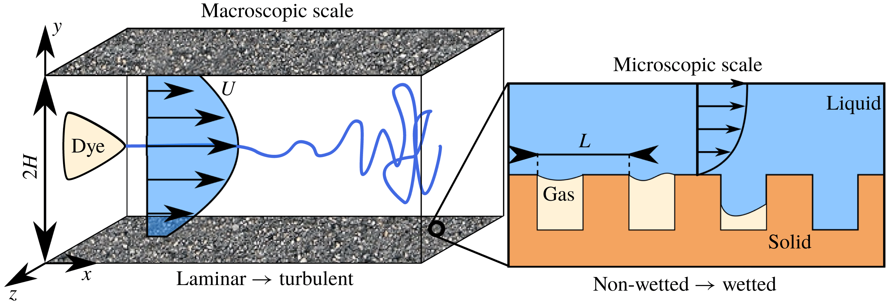
Sketch of a channel flow bounded with submerged superhydrophobic surfaces, depicting the length–scales gap between the overlying laminar–turbulent macroscopic flow and the near-wall, capillary-driven microscopic free-surface dynamics. Laminar–turbulent transition occurs at the macroscopic scale
 $H$
, while Cassie–Baxter/Wenzel transition, where gas bubbles are depleted leading to surface wetting, occurs at the microscopic one,
 $L$
. Here
 $x,z,y$
denote the streamwise, spanwise and wall-normal directions, respectively.

Even though such approximations allow for the use of the single phase, incompressible Navier–Stokes equations, accurate simulations remain computationally demanding (Seo & Mani Reference Seo and Mani2016). In fact, one has to numerically solve both the macroscopic laminar–turbulent bulk flow having the scale of the channel half-height
 $H$
, as well as the microscopic dynamics at the scale of the texture roughnesses,
 $L$
, as depicted in the sketch of figure 1, where
 $x$
,
 $y$
,
 $z$
represent the streamwise, wall-normal and spanwise directions respectively. Whilst for laminar flows in microchannels the
 $H/L$
ratio is of order
 ${\approx}10$
(Byun et al.
Reference Byun, Kim, Ko and Park2008), it can easily reach
 ${\approx}1000$
in finite-size channels (of interest here) for ensuring wetting-stable conditions, (Daniello et al.
Reference Daniello, Waterhouse and Rothstein2009; Zhang et al.
Reference Zhang, Yao and Hao2016; Rowin et al.
Reference Rowin, Hou and Ghaemi2017), considerably increasing the computational cost of the problem. In the last decades, a number of theoretical and numerical studies, both in laminar (Tretheway & Meinhart Reference Tretheway and Meinhart2002; Choi, Westin & Breuer Reference Choi, Westin and Breuer2003; Ou et al.
Reference Ou, Perot and Rothstein2004) and turbulent flows (Daniello et al.
Reference Daniello, Waterhouse and Rothstein2009; Rosenberg et al.
Reference Rosenberg, Van Buren, Fu and Smits2016; Seo & Mani Reference Seo and Mani2016) have established that these alternating, spatially heterogeneous slip/no-slip boundary condition patterns can be effectively modelled via an equivalent spatially homogeneous Robin boundary condition
 $$\begin{eqnarray}U=L_{s}\frac{\unicode[STIX]{x2202}U}{\unicode[STIX]{x2202}y},\quad V=0,\quad w=L_{s}\frac{\unicode[STIX]{x2202}W}{\unicode[STIX]{x2202}y},\end{eqnarray}$$
where
 $[u,w]$
and
 $\unicode[STIX]{x2202}[u,w]/\unicode[STIX]{x2202}y$
are the slip velocity and the shear rate in the wall-normal direction
 $y$
at the boundary
 $(y=\pm 1)$
, while
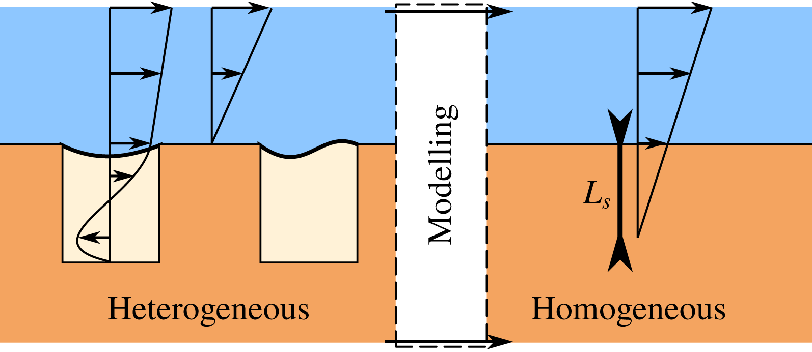
 $L_{s}$
denotes the slip length, as sketched in figure 2. While a number of studies take into account an anisotropic slip length (Min & Kim Reference Min and Kim2004; Aghdam & Ricco Reference Aghdam and Ricco2016; Pralits, Alinovi & Bottaro Reference Pralits, Alinovi and Bottaro2017), here we will consider surfaces that are statistically homogeneous in all wall-parallel directions, therefore allowing for the use of a single isotropic slip length
 $L_{s}$
which, together with a standard non-permeable assumption (
 $v=0$
), will constitute the framework of the present work. This approach, similar to that recently proposed by Zampogna, Magnaudet & Bottaro (Reference Zampogna, Magnaudet and Bottaro2019) for rough walls, allows for a huge reduction of the computational cost of a direct numerical simulation (DNS) of channel flow: Seo & Mani (Reference Seo and Mani2016) have recently shown that a DNS using heterogeneous slip/no-slip boundary conditions would need a
 $12$
times more refined computational grid compared to an equivalent computation using a homogeneous slip boundary condition. Recent DNS of turbulent flows over spatially heterogeneous boundary conditions, resolved up to the scale of the texture roughness (Seo & Mani Reference Seo and Mani2016), have confirmed the trend found in experiments for both laminar (Choi et al.
Reference Choi, Westin and Breuer2003; Ou et al.
Reference Ou, Perot and Rothstein2004) and turbulent regimes (Daniello et al.
Reference Daniello, Waterhouse and Rothstein2009; Zhang et al.
Reference Zhang, Tian, Yao, Hao and Jiang2015, Reference Zhang, Yao and Hao2016), as well as the theoretical predictions by Fukagata et al. (Reference Fukagata, Kasagi and Koumoutsakos2006), Seo & Mani (Reference Seo and Mani2018). Given the texture geometry, in most flow conditions the slip length
 $L_{s}$
is linearly dependent on the texture characteristic size
 $L$
, up to a threshold value for which the high shear and pressure fluctuations will induce gas bubble depletion, resulting in a wetted (Wenzel Reference Wenzel1936) state, providing an overall increase of the drag (Zhang et al.
Reference Zhang, Yao and Hao2016; Seo et al.
Reference Seo, García-Mayoral and Mani2017; Gose et al.
Reference Gose, Golovin, Boban, Mabry, Tuteja, Perlin and Ceccio2018).
Sketch of a channel flow with submerged superhydrophobic surfaces, depicting the near-wall, capillary-driven microscopic free-surface dynamics as well as its modelling using a slip condition with slip length
 $L_{s}$
. In the homogeneous case the slip is modelled using a Robin condition relating the wall-parallel velocities to their derivatives in the wall-normal direction
 $y$
through the slip length
 $L_{s}$
.

1.3 Controlling laminar–turbulent transition using superhydrophobic surfaces
While the influence of superhydrophobic surfaces as a mean of passive flow control has been extensively studied in the laminar and turbulent regimes, to the authors knowledge, only few studies have until now focused on the impact of SHS on the laminar–turbulent transition process. Watanabe, Yanuar & Udagawa (Reference Watanabe and Udagawa1999) have been amongst the first to report on the potential of superhydrophobic surfaces in delaying the onset of transition. Using their experimental pipe flow facility they found that the transition Reynolds number increased with a superhydrophobic coating, indicating that fluid slip could extend the range of stability of the laminar state. The first linear stability analysis of a channel flow with superhydrophobic walls modelled with a spatially homogeneous Robin boundary condition was reported by Min & Kim (Reference Min and Kim2005), who found that introducing slip stabilises the Tollmien–Schlichting waves. This effect was attributed to the shear reduction, and similar results have been found accounting for anisotropic surfaces (Pralits et al. Reference Pralits, Alinovi and Bottaro2017; Alinovi Reference Alinovi2018). In a two-dimensional framework, local stability analyses have been carried out by Donati (Reference De Donati2015), Yu, Teo & Khoo (Reference Yu, Teo and Khoo2016) in streamwise homogeneous configurations. A global stability analysis has been carried out for the flow over a bluff body by Auteri et al. (Reference Auteri, Carini, Fournié, Fratantonio and Giannetti2016), who attributed the flow stabilisation to the shear reduction. Using homogeneous slip as the boundary condition, Min & Kim (Reference Min and Kim2005) investigated the effect of the imposed slip length on a specific transition path, the K-type scenario (Zang & Krist Reference Zang and Krist1989) in a series of direct numerical simulations. They showed that in this particular scenario transition can be delayed by using a slippery boundary condition, but they did not explain how or why this effect is achieved nor did they investigate which physical mechanism is inhibited or damped by the presence of a superhydrophobic surface. This point is particularly interesting and worth investigating since it can potentially provide the key for avoiding transition in specific flow conditions, leading to a considerable drop of the drag. Moreover, since the laminar–turbulent transition path is strongly dependent on the initial disturbances affecting the flow (Reddy et al. Reference Reddy, Schmid, Baggett and Henningson1998), it remains to be investigated in which flow conditions transition delay, and the consequent drag reduction, can be actually achieved.
In this framework, extending the seminal work of Min & Kim (Reference Min and Kim2005), the present work aims at studying how SHS affect transition from laminar to turbulent flow in a channel, for a number of different transition scenarios. The DNS with homogeneous slip conditions are used in order to make a direct validation with the available literature results provided by Min & Kim (Reference Min and Kim2004, Reference Min and Kim2005). Although this simplified approach has been verified and validated in a number of recent studies (Maali & Bhushan Reference Maali and Bhushan2012; Schnitzer & Yariv Reference Schnitzer and Yariv2018; Xu, Crick & Poole Reference Xu, Crick and Poole2018), it is important to choose wisely the main parameters of the problem (gas–solid fraction, scale ratio
 $H/L$
, Weber number etc.) in order to numerically reproduce a flow configuration in which the complex phenomena of shear-driven drainage (Wexler et al.
Reference Wexler, Jacobi and Stone2015; Liu et al.
Reference Liu, Wexler, Schönecker and Stone2016), hydrostatic pressure and air dissolution (Lee & Kim Reference Lee and Kim2011; Duan Reference Duan2017; Xiang et al.
Reference Xiang, Huang, Lv, Xue, Su and Duan2017), stagnation and capillary pressure (Seo & Mani Reference Seo and Mani2016, Reference Seo and Mani2018) may arise, leading to Cassie–Baxter/Wenzel transition, with a deterioration of the lubricating plastron layer. Thus, to choose suitable values of the slip length (i.e. sufficiently low to ensure wetting-stable conditions) we have referred to both experimental (Daniello et al.
Reference Daniello, Waterhouse and Rothstein2009; Rowin et al.
Reference Rowin, Hou and Ghaemi2017; Gose et al.
Reference Gose, Golovin, Boban, Mabry, Tuteja, Perlin and Ceccio2018) and numerical studies (Seo et al.
Reference Seo, García-Mayoral and Mani2017; Seo & Mani Reference Seo and Mani2018) which reported typical values of
 $L_{s}$
achieved for fully turbulent flows while ensuring wetting-stable SHS.
We show that the effectiveness of a SHS in delaying transition is not only related to the amount of slip it can reliably provide, but also onto the specific transition scenario undertaken by the flow. In fact, although transition triggered by near-wall modal perturbations is delayed or even avoided by SHS, the introduction of a slip length is completely ineffective in controlling transition initiated by external noise or by optimal disturbances.
The present manuscript is organised as follows. In § 2.2 we present the fully nonlinear governing equations, as well as their linearised counterpart for setting up the linear stability analysis. In § 3 we show how two modal transition scenarios, both triggered by Tollmien–Schlichting waves in supercritical and subcritical conditions, are influenced by SHS. Section 3.2 contains a thorough investigation of the physical mechanisms leading to delayed K-type transition in the case of a slippery wall, while in § 4 we show that such surfaces are ineffective in controlling transition initiated by external noise or by optimal disturbances. A final discussion and conclusions are given in § 5.
2 Governing equations
The dynamics of an incompressible Newtonian fluid flowing in a channel is governed by the Navier–Stokes equations
 $$\begin{eqnarray}\displaystyle & \displaystyle \frac{\unicode[STIX]{x2202}\boldsymbol{U}}{\unicode[STIX]{x2202}t}=-(\boldsymbol{U}\boldsymbol{\cdot }\unicode[STIX]{x1D735})\boldsymbol{U}-\unicode[STIX]{x1D735}P+\frac{1}{Re}\unicode[STIX]{x1D6FB}^{2}\boldsymbol{U} & \displaystyle\end{eqnarray}$$
 $$\begin{eqnarray}\displaystyle & \displaystyle \unicode[STIX]{x1D735}\boldsymbol{\cdot }\boldsymbol{U}=0, & \displaystyle\end{eqnarray}$$
where
 $\boldsymbol{U}=(U(\boldsymbol{x},t),V(\boldsymbol{x},t),W(\boldsymbol{x},t))^{\text{T}}$
is the velocity field and
 $P(\boldsymbol{x},t)$
is the pressure field. The Reynolds number is defined as
 $Re=U_{r}H/\unicode[STIX]{x1D708}$
, the reference velocity
 $U_{r}=3U_{a}/2$
being the average of the base flow velocity over the entire domain
 $U_{a}=1/2H\int U\,\text{d}x\,\text{d}y\,\text{d}z$
,
 $H$
being half the height of the channel and
 $\unicode[STIX]{x1D708}$
the kinematic viscosity of the fluid. Dimensionless time is therefore
 $t=H/U_{r}$
. The reference frame
 $\boldsymbol{x}=(x,y,z)^{\text{T}}$
is chosen so that
 $x$
is the streamwise,
 $y$
the wall-normal and
 $z$
the spanwise direction.
Steady solutions
 $\boldsymbol{Q}_{b}(\boldsymbol{x})=(\boldsymbol{U}_{b},P_{b})^{\text{T}}$
of the Navier–Stokes equations are known as base flows or fixed points of the system. Under the assumption of small-amplitude disturbances, we decompose the flow field as a sum of the base flow and a perturbation such as
 $\boldsymbol{Q}(\boldsymbol{x},t)=\boldsymbol{Q}_{b}(\boldsymbol{x})+\unicode[STIX]{x1D700}\boldsymbol{q}(\boldsymbol{x},t)$
, with
 $\unicode[STIX]{x1D700}\ll 1$
, that is to say
 $(\boldsymbol{U}(\boldsymbol{x},t),P(\boldsymbol{x},t))^{\text{T}}=(\boldsymbol{U}_{b}(\boldsymbol{x})P_{b}(\boldsymbol{x}))^{\text{T}}+\unicode[STIX]{x1D700}(\boldsymbol{u}(\boldsymbol{x},t),p(\boldsymbol{x},t))^{\text{T}}$
. As will be discussed in the following subsection, the presence of SHS is taken into account using an ad hoc boundary condition at the wall, provided in (1.1). Within this framework, the base flow assumes the form
 $\boldsymbol{U}_{b}(\boldsymbol{x})=(U_{b}(y),0,0)$
, with
 $$\begin{eqnarray}U_{b}(y)=\frac{2L_{s}+1-y^{2}}{3L_{s}+1},\end{eqnarray}$$
as found by Philip (Reference Philip1972). Notice that the centreline velocity, classically used as a reference velocity in channel flows, changes with the slip length. This explains the choice of
 $U_{r}$
as a reference velocity instead of
 $U_{b}(y=0)$
, since it allows us to maintain a constant Reynolds number when changing the slip length for fixed flow rate. In order to trigger transition to turbulence starting from the laminar base flow, we will use perturbations constructed on the basis of modal and non-modal linear stability analyses (see Min & Kim (Reference Min and Kim2005) and Pralits et al. (Reference Pralits, Alinovi and Bottaro2017)).
2.1 Representativity of the partial slip model
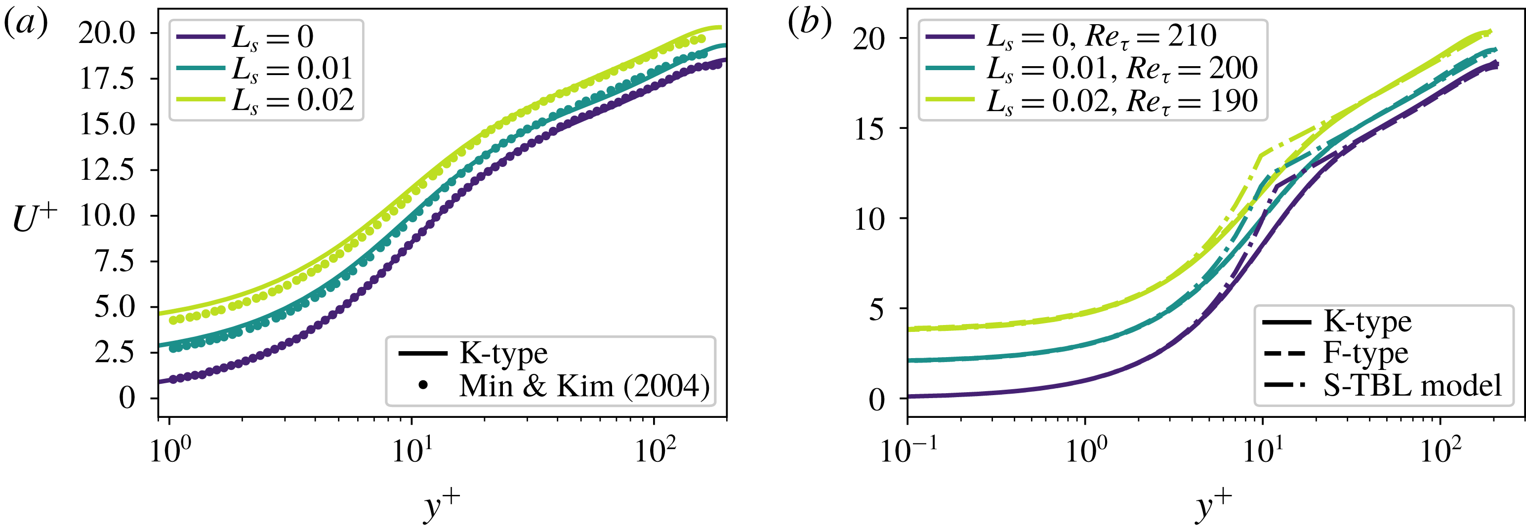
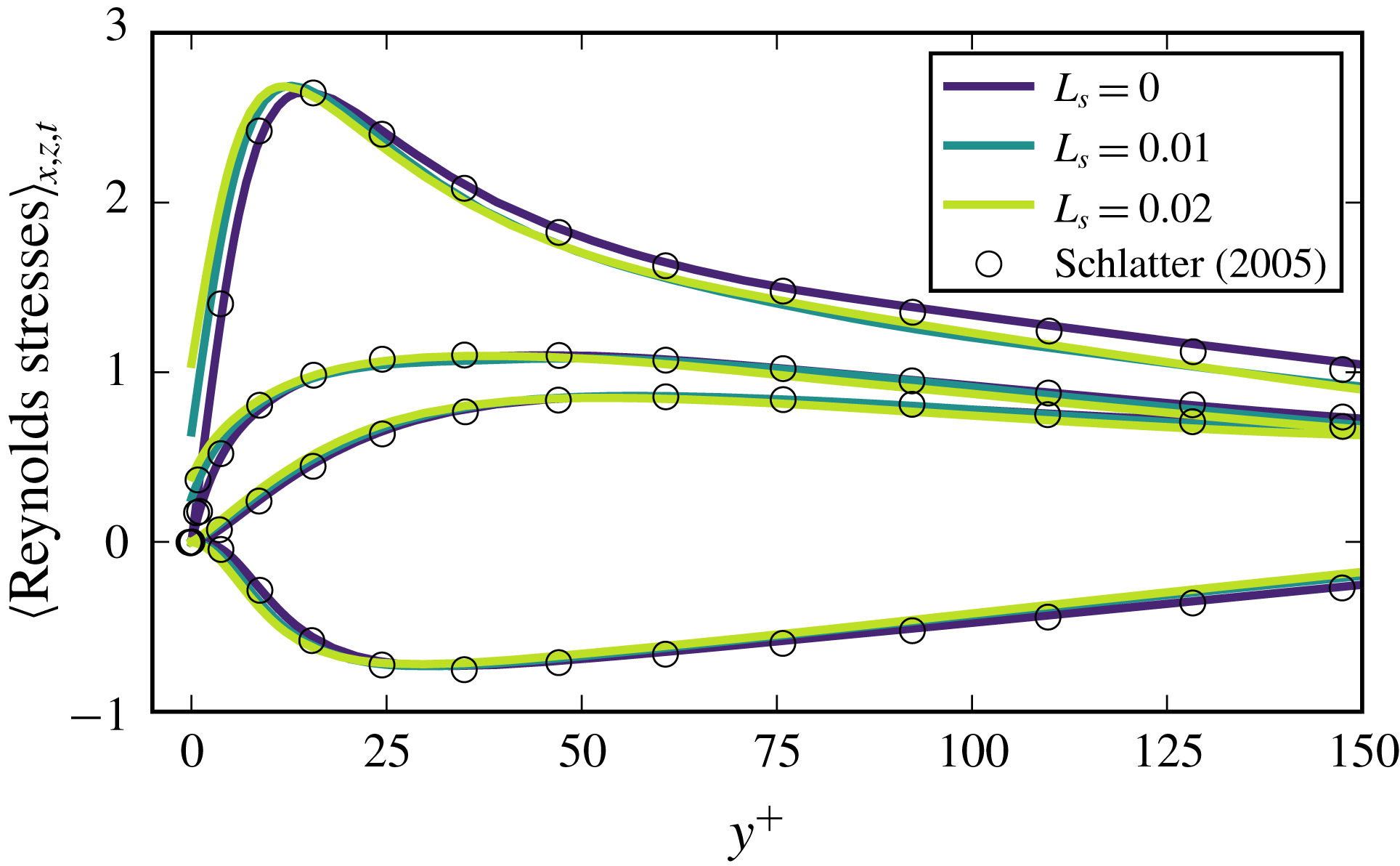
As in the pioneering work of Min & Kim (Reference Min and Kim2004, Reference Min and Kim2005), in this paper the presence of a submerged superhydrophobic surface has been modelled using a spatially homogeneous partial slip boundary condition. As will be discussed in the following, when the spanwise length of the grooves and the shear-free fraction are sufficiently small with respect to the channel thickness, so to retain the lubricating layer within the surface micro-roughnesses even in transitional/turbulent conditions (Seo & Mani Reference Seo and Mani2016), this simple partial slip condition allows us to model accurately enough the macroscopic flow behaviour observed in experimental essays.
In this work, slip length values of
 $L_{s}=0.005,0.01,0.02$
have been considered in order to match the values employed by Min & Kim (Reference Min and Kim2005), enabling a direct comparison of our results with those in the literature. However, we should verify that these slip length values can be realistically obtained by microtextured SHS in wetting-stable conditions. Equation (15) of the recent work by Seo & Mani (Reference Seo and Mani2016) allows us to determine the equivalent slip length
 $L_{s}$
provided by a microtextured superhydrophobic surface, given the geometrical pattern and the length scale
 $L$
of the micro roughness. Combining equations (3) and (15) from Seo & Mani (Reference Seo and Mani2016) we obtain
 $$\begin{eqnarray}L^{+}=\frac{L_{s}^{+}\sqrt{\unicode[STIX]{x1D719}_{s}}}{0.325-0.44\sqrt{\unicode[STIX]{x1D719}_{s}}}+0.328(L_{s}^{+}\sqrt{\unicode[STIX]{x1D719}_{s}})^{3},\end{eqnarray}$$
where
 $L^{+}=LRe_{\unicode[STIX]{x1D70F}}$
and
 $L_{s}^{+}=L_{s}Re_{\unicode[STIX]{x1D70F}}$
, respectively,
 $Re_{\unicode[STIX]{x1D70F}}=u_{\unicode[STIX]{x1D70F}}H/\unicode[STIX]{x1D708}$
being the friction Reynolds number, and
 $\unicode[STIX]{x1D719}_{s}$
is the solid fraction, quantifying the fraction of solid contact within the SHS roughness pattern, typically spanning from
 $0.1$
to
 $0.3$
(Bidkar et al.
Reference Bidkar, Leblanc, Kulkarni, Bahadur, Ceccio and Perlin2014; Zhang et al.
Reference Zhang, Yao and Hao2016). For the purposes of this section, we have set
 $\unicode[STIX]{x1D719}_{s}=0.25$
. Using this equation we evaluate the equivalent roughness size required to obtain the largest slip length considered here,
 $L_{s}=0.02$
, for which an undesired depletion of the plastron layer might be more likely to occur (Zhang et al.
Reference Zhang, Yao and Hao2016). Setting
 $\unicode[STIX]{x1D719}_{s}=0.25$
and
 $Re_{\unicode[STIX]{x1D70F}}\approx 200$
(as obtained by Min & Kim (Reference Min and Kim2005) for the same flow configuration used in the present work), the largest equivalent texture size attains
 $L^{+}\approx 19$
. This value complies with the conditions discussed by Seo et al. (Reference Seo, García-Mayoral and Mani2017) to avoid wetting transition, either triggered by capillarity or stagnation pressure. Moreover, the equivalent texture size
 $L^{+}$
is small enough to not interact with the overlying coherent structures characteristic of a turbulent flow (Fairhall et al.
Reference Fairhall, Abderrahaman-Elena and García-Mayoral2018), which have a length scale which is typically of
 $O(100)$
(Lee, Eckelman & Hanratty Reference Lee, Eckelman and Hanratty1974). These conditions ensure that the simple spatially homogeneous partial slip employed in the present study would provide virtually the same result that a heterogeneous alternation of slip/no-slip patches, both in laminar (Ybert et al.
Reference Ybert, Barentin, Cottin-Bizonne, Joseph and Bocquet2007) and in fully turbulent flows (Seo & Mani Reference Seo and Mani2016). Finally, imposing an
 $L^{+}$
of
 $O(10)$
leads to a micro-roughness size comparable with those characterising superhydrophobic surfaces successfully employed in experimental campaigns (Daniello et al.
Reference Daniello, Waterhouse and Rothstein2009; Zhang et al.
Reference Zhang, Yao and Hao2016; Gose et al.
Reference Gose, Golovin, Boban, Mabry, Tuteja, Perlin and Ceccio2018). Using slip lengths larger than
 $L_{s}=0.02$
would enhance the effect of surface slip, but lead to an increase of the equivalent roughness size that must not exceed that of superhydrophobic surfaces characterised by contact angle hysteresis in the
 $5^{\circ }{-}10^{\circ }$
range (Zhang et al.
Reference Zhang, Yao and Hao2016; Gose et al.
Reference Gose, Golovin, Boban, Mabry, Tuteja, Perlin and Ceccio2018), capable of successfully sustaining a fully developed turbulent flow.
2.2 Linear stability analysis (LSA)
Linearising the governing equations around the base flow we obtain the linearised Navier–Stokes equations, which, once projected onto a divergence-free vector space, can be compactly written as
 $$\begin{eqnarray}\frac{\unicode[STIX]{x2202}\boldsymbol{u}}{\unicode[STIX]{x2202}t}=\boldsymbol{L}\boldsymbol{u},\end{eqnarray}$$
together with the linearised wall boundary conditions:
 $$\begin{eqnarray}u=L_{s}\frac{\unicode[STIX]{x2202}u}{\unicode[STIX]{x2202}y},\quad v=0,\quad w=L_{s}\frac{\unicode[STIX]{x2202}w}{\unicode[STIX]{x2202}y},\end{eqnarray}$$
 $u,v,w$
being the streamwise, wall-normal and spanwise components of the velocity perturbation, respectively. With this system being autonomous in time and the base flow being periodic in both the streamwise and spanwise directions, one can apply a Fourier–Laplace transform to any field
 $\boldsymbol{q}$
so that
 $\boldsymbol{q}(\boldsymbol{x},t)=\tilde{\boldsymbol{q}}(y)\exp [\text{i}(\unicode[STIX]{x1D6FC}x+\unicode[STIX]{x1D6FD}z)+\unicode[STIX]{x1D706}t]+\text{c.c.}$
, where
 $\text{c.c.}$
is the complex conjugate,
 $\unicode[STIX]{x1D6FC}$
and
 $\unicode[STIX]{x1D6FD}$
are the real streamwise and spanwise wavenumbers, respectively,
 $\unicode[STIX]{x1D706}$
is the complex circular frequency and
 $\tilde{\boldsymbol{q}}\in \mathbb{C}^{4}$
is the associated eigenfunction.
In this framework, the behaviour of a generic solenoidal perturbation
 $\boldsymbol{u}$
is linked to the eigenpairs of
 $\boldsymbol{L}$
:
 $\{\unicode[STIX]{x1D706}^{eig},\tilde{\boldsymbol{u}}^{eig}\}$
(Orszag Reference Orszag1971), since they can be written as
 $$\begin{eqnarray}\boldsymbol{u}(\boldsymbol{x},t)=\mathop{\sum }_{l}\unicode[STIX]{x1D705}_{l}\tilde{\boldsymbol{u}}(y)_{l}^{eig}\exp (\text{i}(\unicode[STIX]{x1D6FC}x+\unicode[STIX]{x1D6FD}z)+\unicode[STIX]{x1D706}_{l}^{eig}t),\end{eqnarray}$$
where
 $\unicode[STIX]{x1D705}_{l}$
is a scalar weight. For a given couple
 $(\unicode[STIX]{x1D6FC},\unicode[STIX]{x1D6FD})$
the temporal behaviour of each eigenvector of the linearised operator
 $\boldsymbol{L}$
is then described by its associated eigenvalue
 $\unicode[STIX]{x1D706}_{i}^{eig}=\unicode[STIX]{x1D70E}_{i}^{eig}+\text{i}\unicode[STIX]{x1D714}_{i}^{eig}$
, where
 $\unicode[STIX]{x1D70E}_{i}^{eig}$
represents its asymptotic growth/decay rate and
 $\unicode[STIX]{x1D714}_{i}^{eig}$
its circular frequency.
Solving the one-dimensional local stability problem, which is to say, seeking the eigenvalues of
 $\boldsymbol{L}$
which govern the behaviour of small perturbations in the time-asymptotic limit, by means of a spectral code (Schmid & Henningson Reference Schmid and Henningson2001), we retrieve the same results found by Min & Kim (Reference Min and Kim2005). The most unstable modes of the operator
 $\boldsymbol{L}$
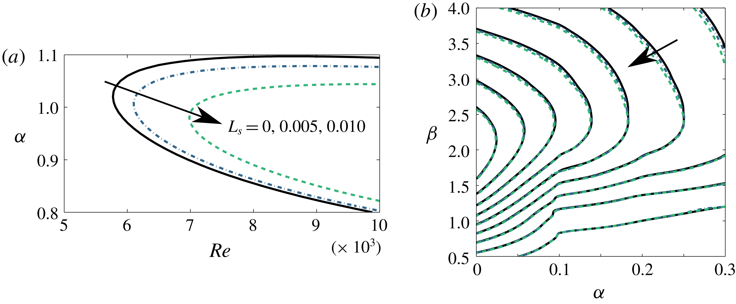
, i.e. the Tollmien–Schlichting (TS) waves, are strongly affected by the value of the slip length imposed at the wall. This is not surprising considering that TS waves are near-wall perturbations and that SHS reduce the velocity gradient near the wall. Figure 3(a) shows, for each considered value of
 $L_{s}$
, the relative neutral curve in the
 $Re{-}\unicode[STIX]{x1D6FC}$
plane, which separates the unstable region of the plane (right side of the curve) from the stable one (left side). Increasing the value of
 $L_{s}$
the neutral curve moves towards higher values of
 $Re$
, suggesting that SHS might delay transition to turbulence, at least in supercritical conditions (i.e. when the Reynolds number overtakes the critical value for linear instability).
In subcritical conditions, small-amplitude perturbations can transiently grow in time due to non-modal mechanisms, linked to the non-normality of the Navier–Stokes equations. To investigate how the non-modal dynamics of small perturbations is affected by SHS in a finite-time framework, we seek the ‘optimal’ perturbation at initial time,
 $\boldsymbol{u}_{0}^{Opt}(\boldsymbol{x})$
, capable of inducing the maximum energy growth at a target time
 $T$
(Butler & Farrell Reference Butler and Farrell1992; Luchini Reference Luchini2000). The energy gain to be optimised reads
 $$\begin{eqnarray}G(T)=\max _{\boldsymbol{u}_{0}}\frac{E(\boldsymbol{u}_{T})}{E(\boldsymbol{u}_{0})},\end{eqnarray}$$
where the integral energy in the computational domain
 $V$
is defined as
 $$\begin{eqnarray}E(\boldsymbol{u}(t))=\frac{1}{2L_{x}L_{z}}\int _{V}\boldsymbol{u}^{\text{T}}(t)\boldsymbol{u}(t)\,\text{d}V.\end{eqnarray}$$
To obtain the optimal energy gain and the corresponding initial and final optimal perturbations
 $\boldsymbol{u}_{0}^{Opt}(\boldsymbol{x})$
,
 $\boldsymbol{u}_{T}^{Opt}(\boldsymbol{x})$
, a singular value decomposition of the linearised governing equation (2.5) has been used, following the approach of Schmid & Brandt (Reference Schmid and Brandt2014). As shown in figure 3(b), a variation of
 $L_{s}$
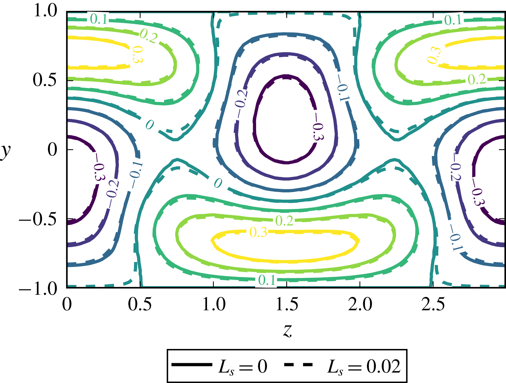
induces but a slight modification of the maximum energy gain and of the optimal perturbation shape, consisting of modulations in the spanwise direction of the streamwise velocity, i.e. streaks (Farrell Reference Farrell1988). In fact, since these optimal structures essentially lie in the flow bulk far from the walls, they are much less affected by the surface boundary condition than the near-wall TS waves. The fact that velocity perturbations are slightly or strongly affected by SHS depending on their distance from the wall suggests that some specific transition scenarios can be better controlled than others through the introduction of SHS.
Linear stability and transient growth analyses for different values of
 $L_{s}$
: neutral curve indicating the
 $Re-\unicode[STIX]{x1D6FC}$
values for which the growth rate of the most unstable mode with
 $\unicode[STIX]{x1D6FD}=0$
is zero (a) and optimal energy gain contours in the
 $\unicode[STIX]{x1D6FC}{-}\unicode[STIX]{x1D6FD}$
plane for
 $Re=1000$
(b), both in perfect match with Min & Kim (Reference Min and Kim2005). The slip length strongly affects the time asymptotic behaviour, while being ineffective in controlling finite-time dynamics, as shown by the unmodified contours of the optimal transient energy growth. Solid, dashed and dashed-dotted contours in (b) are related to the same values of
 $L_{s}$
reported in (a). The values of the isocontours in (b), from outer to inner, correspond to
 $G_{max}=[110,120,130,\ldots ,180,190,200]$
.

2.3 Direct numerical simulations
In order to investigate the influence of SHS on laminar–turbulent transition, we superpose different perturbations built on the basis of the previously introduced modal and non-modal stability analyses to the laminar base flow and follow their evolution using DNS. The flow in a streamwise-periodic channel with constant flow rate is simulated using the incompressible solver Nek5000 (Fischer, Lottes & Kerkemeier Reference Fischer, Lottes and Kerkemeier2008), based on the spectral element method. The code, which has been modified in order to account for the Robin boundary condition (1.1) (see the supplementary material for some details of the implementation) is based on a
 $\mathbb{P}_{N}-\mathbb{P}_{N-2}$
spatial discretisation. Viscous terms are advanced in time using a backward differentiation of order 3, whereas for convective terms an extrapolation of order 3 is used, resulting in the time-advancement scheme labelled BDF3/EXT3. Throughout the present work, the domain size is set to
 $[L_{x},L_{y},L_{z}]=[2\unicode[STIX]{x03C0}/\unicode[STIX]{x1D6FC},2H,2\unicode[STIX]{x03C0}/\unicode[STIX]{x1D6FD}]$
, where, unless otherwise stated, we have imposed
 $\unicode[STIX]{x1D6FC}=1.12,\unicode[STIX]{x1D6FD}=2.10$
to match the domain size typically employed to study K-type transition in a channel flow (Zang & Krist Reference Zang and Krist1989; Sandham & Kleiser Reference Sandham and Kleiser1992; Min & Kim Reference Min and Kim2005; Schlatter Reference Schlatter2005). In most of the computations the Reynolds number is set to
 $Re=5000$
in order to match literature results about K-type transition in channel flows (Zang & Krist Reference Zang and Krist1989). Using 24 spectral elements in each direction with a polynomial order equal to 8, the resulting spatial resolution is
 $[N_{x},N_{y},N_{z}]=[192,192,192]$
. Under these conditions and considering a no-slip wall, the resulting fully turbulent state is characterised by a friction Reynolds number
 $Re_{\unicode[STIX]{x1D70F}}=210$
(Schlatter, Stolz & Kleiser Reference Schlatter, Stolz and Kleiser2006) (albeit we will show that imposing a constant flow rate will result in a lower
 $Re_{\unicode[STIX]{x1D70F}}$
for a turbulent flow over SHS). Therefore, the grid size expressed in friction units is sufficiently small to accurately simulate a turbulent channel flow by means of DNS (Seo & Mani Reference Seo and Mani2018). In particular we have
 $\unicode[STIX]{x0394}x^{+}\approx 6.2,\unicode[STIX]{x0394}z^{+}\approx 3.0$
,
 $\unicode[STIX]{x0394}y_{min}^{+}\approx 0.16$
at the wall and
 $\unicode[STIX]{x0394}y_{max}^{+}\approx 11.5$
at the centreline, which are lower than the values used by Min & Kim (Reference Min and Kim2004, Reference Min and Kim2005).
3 Transition triggered by modal mechanisms
The aim of the present work is to explain how different scenarios of transition to turbulence are affected by a slip boundary condition with given slip length. First, we consider the case in which transition is triggered by modal stability mechanisms. Thus, following Zang & Krist (Reference Zang and Krist1989), Sandham & Kleiser (Reference Sandham and Kleiser1992), Schlatter et al. (Reference Schlatter, Stolz and Kleiser2006), we use as initial condition for the DNS a superposition of the laminar base flow plus a linear combination of eigenvectors of
 $\boldsymbol{L}$
,
 $$\begin{eqnarray}\boldsymbol{U}(\boldsymbol{x},t=0)=\boldsymbol{U}_{b}(\boldsymbol{x})+\mathop{\sum }_{j}\unicode[STIX]{x1D716}_{j}\tilde{\boldsymbol{u}}(y)_{j}^{eig}\exp (\text{i}(\unicode[STIX]{x1D6FC}x+\unicode[STIX]{x1D6FD}z)+\unicode[STIX]{x1D706}_{j}^{eig}t),\end{eqnarray}$$
where
 $\unicode[STIX]{x1D716}_{j}$
is a given scalar amplitude. In supercritical conditions, namely for
 $Re\geqslant Re_{critical}=5772.22$
(Orszag Reference Orszag1971), only one mode will be retained on the right-hand side of the previous equation, namely the most unstable one. Whereas, in subcritical conditions (Zang & Krist Reference Zang and Krist1989), we will refer to the well-known K-type (or H-type) transition (Kachanov Reference Kachanov1994), that can be obtained numerically by setting initial conditions similar to the experiments of Nishioka, Iid & Ichikawa (Reference Nishioka, Iid and Ichikawa1975), where a sum of two-dimensional and oblique TS waves were used (Kleiser & Zang Reference Kleiser and Zang1991). In the literature, the effects of SHS on transition to turbulence have been studied for the K-type scenario only (see Min & Kim (Reference Min and Kim2005)), but even for this case the physical mechanisms leading to transition delay have not been investigated yet.
3.1 Supercritical case: TS waves
First, we study how slippery boundaries can affect the laminar–turbulent transition process when
 $Re\geqslant Re_{critical}$
, namely in the supercritical regime. Thus, for the computations presented in this paragraph we set
 $Re=10\,000$
,
 $\unicode[STIX]{x1D6FC}=1.0$
and
 $\unicode[STIX]{x1D6FD}=2.0$
, to ensure a linearly unstable flow even for a large slip length, see figure 3(a). In these flow conditions, the most unstable eigenvalue of
 $\boldsymbol{L}$
is the two-dimensional TS wave with
 $\unicode[STIX]{x1D6FC}=1.00,\unicode[STIX]{x1D6FD}=0.0$
, which we will refer to as
 $\boldsymbol{u}_{TS_{2D}}$
. Supercritical transition is triggered using as initial condition this unstable mode superposed on the base flow as
 $\boldsymbol{U}(\boldsymbol{x},t=0)=\boldsymbol{U}_{b}(\boldsymbol{x})+\unicode[STIX]{x1D716}\boldsymbol{u}_{TS_{2D}}(\boldsymbol{x})$
first for a no-slip wall and then for a slip value compatible with the experiments of Gose et al. (Reference Gose, Golovin, Boban, Mabry, Tuteja, Perlin and Ceccio2018), namely
 $L_{s}=0.005$
. The amplitude
 $\unicode[STIX]{x1D716}$
is set to
 ${\approx}3\times 10^{-3}$
to guarantee an initial phase of exponential growth before the onset of nonlinear effects, provided that
 $E(t=0)=10^{-5}$
.
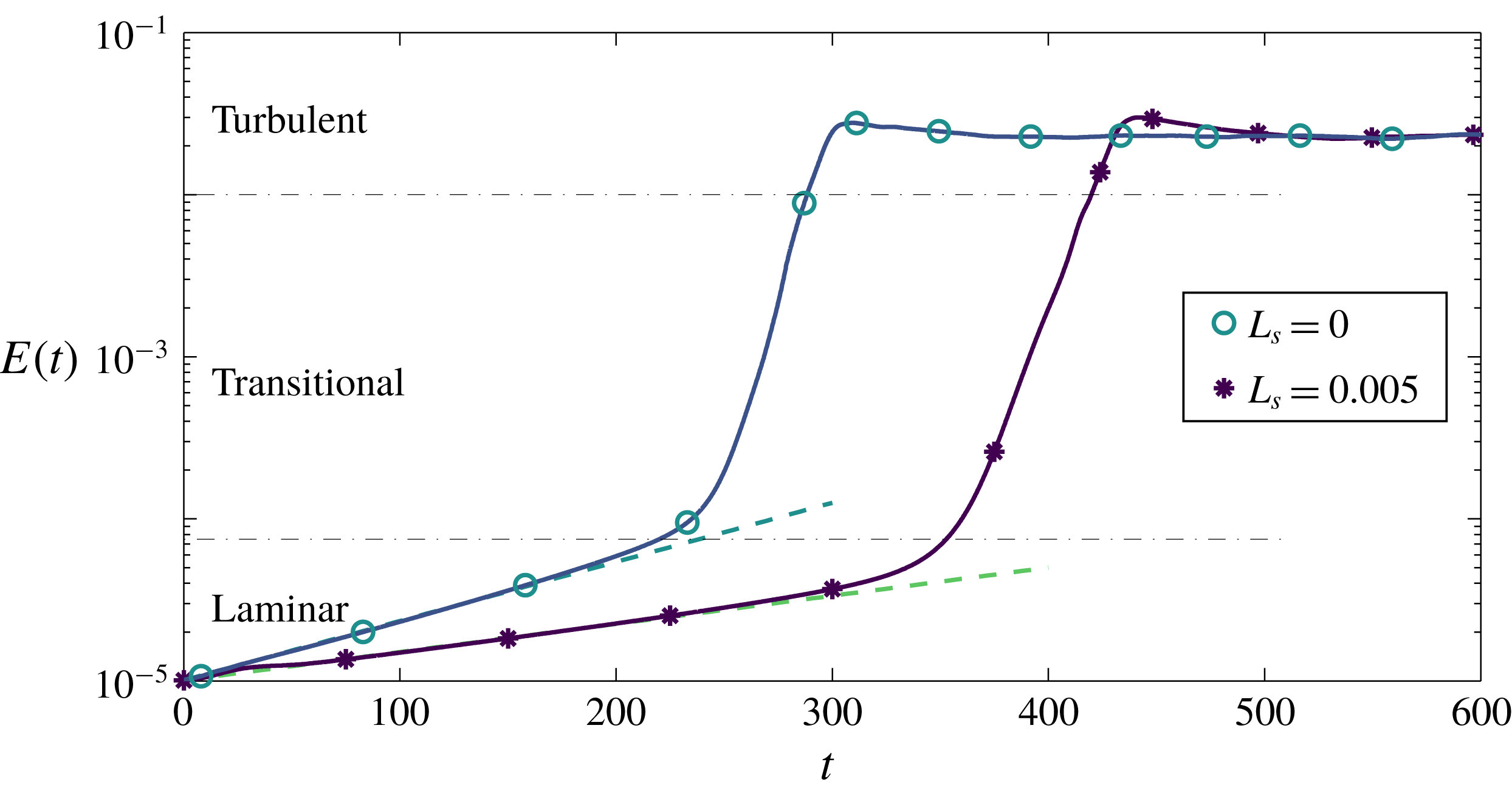
In order to detect transition we track the evolution of the kinetic energy density of the velocity perturbation defined in (2.9). The result is plotted in figure 4 for
 $L_{s}=0$
and
 $L_{s}=0.005$
. In both cases, after an initial phase characterised by exponential growth, as predicted by the LSA, secondary instability sets in, leading to a rapid increment of
 $E$
towards saturation to a fully turbulent state. For both the considered values of
 $L_{s}$
the onset of secondary instability is observed for
 $E\approx 5\times 10^{-5}$
, and the energy saturates towards the same value characterising the turbulent regime. The initial phase of linear amplification of the perturbation energy density matches the predictions of the linear stability theory, as one can notice comparing the DNS results (solid lines) with the dashed lines representing an exponential energy growth with exponent
 $2\unicode[STIX]{x1D70E}$
,
 $\unicode[STIX]{x1D70E}$
being the growth rate of the most unstable eigenmode of
 $\boldsymbol{L}$
. As predicted by LSA, in the presence of SHS, the initial exponential phase is characterised by a lower growth rate, thus the threshold energy for secondary instability is reached in more time, leading to a time delay of the consequent transition to turbulence. For the chosen amplitude of the unstable mode, most of the transition time is spent during the initial exponential growth and the physical mechanisms leading to transition are essentially the same in both the considered cases. Therefore, the transition time might be estimated using the
 $e^{N}$
method (van Ingen Reference van Ingen2008) also for the SHS case.
Influence of SHS on the supercritical transition path at
 $Re=10\,000$
. Simulations have been initialised with the most unstable eigenvector of
 $\boldsymbol{L}$
, with initial perturbation kinetic energy density equal to
 $E(t)=10^{-5}$
, for different slip lengths
 $L_{s}$
. The initial linear amplification phase matches the prediction of the linear stability theory as shown by the dashed lines with slopes equal to
 $2\unicode[STIX]{x1D70E}$
, with
 $\unicode[STIX]{x1D70E}(L_{s}=0.000)\approx 0.00374$
and
 $\unicode[STIX]{x1D70E}(L_{s}=0.005)\approx 0.002978$
, where
 $\unicode[STIX]{x1D70E}$
is the growth rate of the most unstable eigenmode of
 $\boldsymbol{L}$
, for
 $\unicode[STIX]{x1D6FC}=1.0,\unicode[STIX]{x1D6FD}=0.0$
and
 $Re=10\,000>Re_{critical}$
.

3.2 Subcritical case: K-type transition
In this section we study in detail how the K-type transition scenario is influenced by a slippery wall at
 $Re=5000$
, pursuing the study made by Min & Kim (Reference Min and Kim2005) in order to unveil the physical mechanisms leading to transition delay in subcritical conditions. Following their work, the K-type transition scenario is triggered setting as initial disturbances a sum of the two-dimensional (2-D) TS wave
 $\boldsymbol{u}_{TS_{2D}}$
with
 $(\unicode[STIX]{x1D6FC},\unicode[STIX]{x1D6FD})=(1.12,0.0)$
, and a sum of equal and opposite oblique three-dimensional (3-D) fundamental Tollmien–Schlichting waves
 $\boldsymbol{u}_{TS_{\pm 3D}}$
characterised by spatial wavenumbers
 $(\unicode[STIX]{x1D6FC},\unicode[STIX]{x1D6FD})=(1.12,\pm 2.10)$
. All the considered TS waves are the most unstable eigenmodes of
 $\boldsymbol{L}$
obtained for the imposed
 $(\unicode[STIX]{x1D6FC},\unicode[STIX]{x1D6FD},Re)$
values using a one-dimensional (1-D) local stability analysis code implementing a Chebyshev spectral collocation approach on a 200 points grid, as indicated in § 2.2. From now on, the domain size is set to
 $[L_{x},L_{y},L_{z}]=[2\unicode[STIX]{x03C0}/\unicode[STIX]{x1D6FC},2H,2\unicode[STIX]{x03C0}/\unicode[STIX]{x1D6FD}]$
, with
 $\unicode[STIX]{x1D6FC}=1.12,\unicode[STIX]{x1D6FD}=2.10$
.
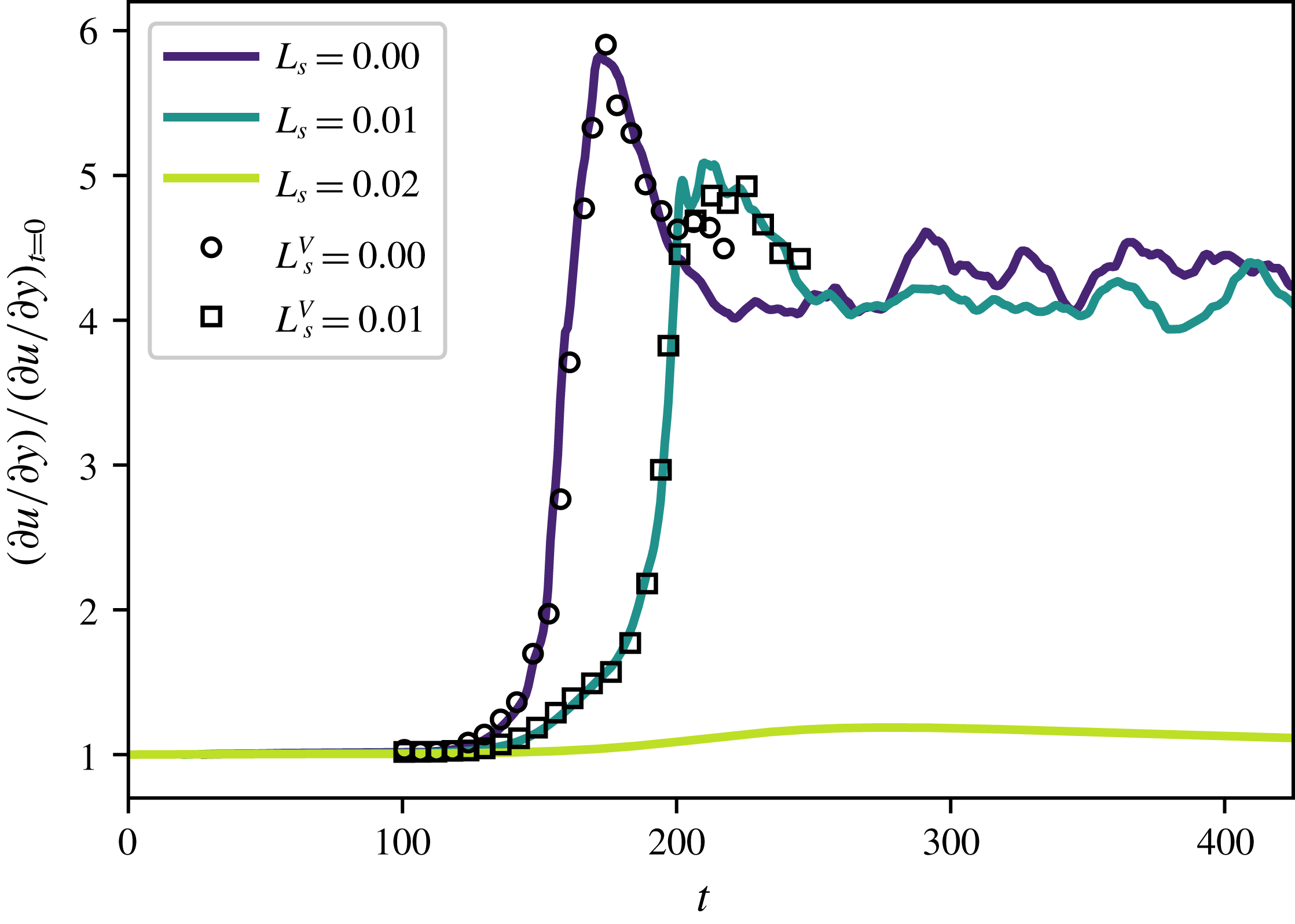
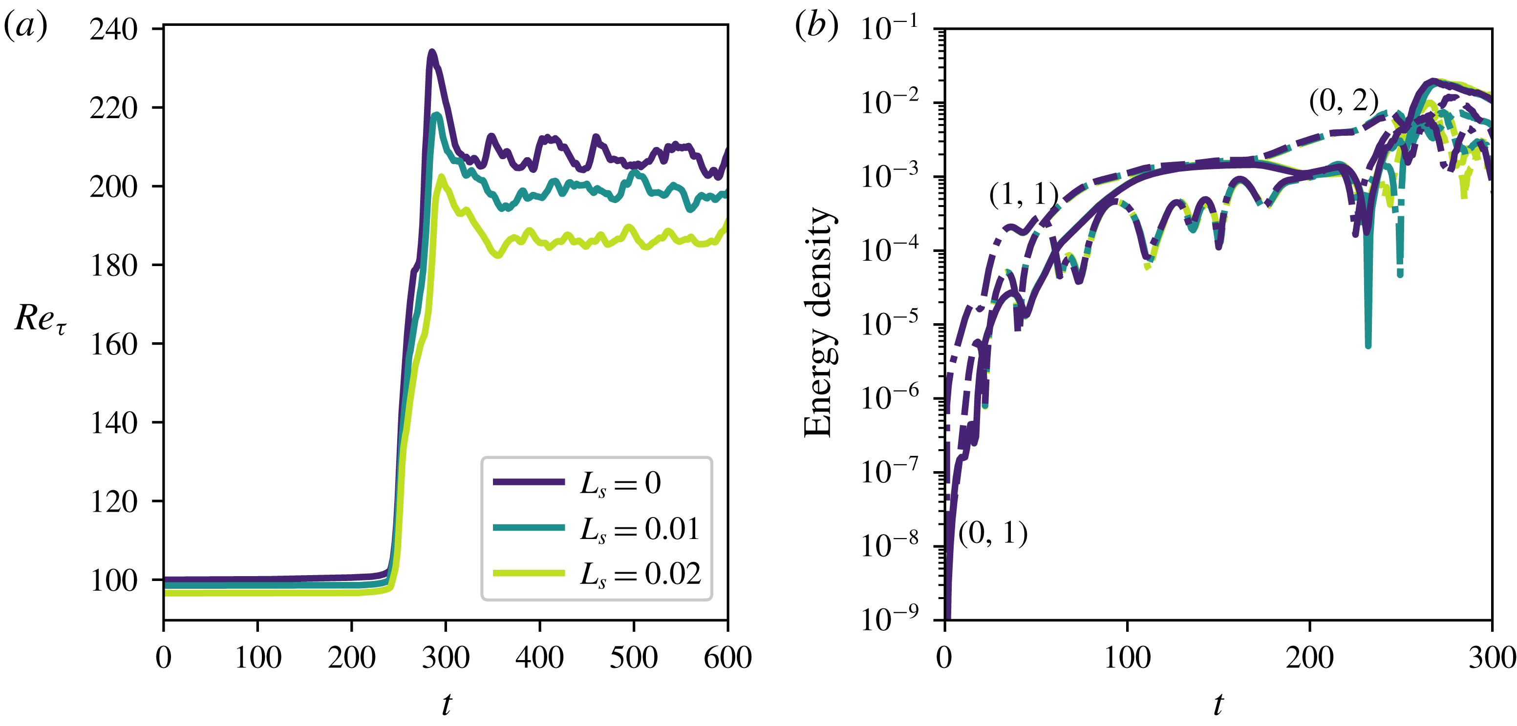
Time evolution of the instantaneous wall shear normalised by its laminar value in a standard K-type transition scenario as in (3.2). Compared to the benchmark no-slip case (
 $L_{s}=0.00$
), using SHS modelled superhydrophobic surfaces transition to turbulence can be retarded (
 $L_{s}=0.01$
) or even avoided (
 $L_{s}=0.02$
). The symbols
 $L_{s}^{V}$
are validations with respect to the case 3 from Min & Kim (Reference Min and Kim2005).

The initial condition for K-type transition (Kleiser & Zang Reference Kleiser and Zang1991; Schlatter Reference Schlatter2005) then reads
 $$\begin{eqnarray}\boldsymbol{U}(t=0)=\boldsymbol{U}_{BF}+0.03\boldsymbol{u}_{TS_{2D}}\pm 0.001\boldsymbol{u}_{TS_{\pm 3D}},\end{eqnarray}$$
where the shape of the modes depends on the imposed value of
 $L_{s}$
and their phase is set so that the maximum amplitude of the disturbances occurs at
 $z=L_{z}/2$
(Zang & Krist Reference Zang and Krist1989; Sandham & Kleiser Reference Sandham and Kleiser1992). For both waves, the maximum value of the streamwise velocity component is set to the desired amplitude and the other components are scaled accordingly. Figure 5 shows the temporal evolution of the instantaneous wall shear normalised by its laminar value for
 $L_{s}=0.00,0.01,0.02$
. The first two curves accurately reproduce those in figure 3(a) of the work by Min & Kim (Reference Min and Kim2005) (where only
 $L_{s}=0.00$
and
 $L_{s}=0.01$
are considered), validating our numerical approach. The highest value of
 $L_{s}=0.02$
, already used by the same authors in a previous study (Min & Kim Reference Min and Kim2004), would result from a SHS having a roughness texture period of
 $L^{+}\approx 15$
in the turbulent regime (Seo & Mani Reference Seo and Mani2016). This value of
 $L^{+}$
is still sufficiently low to ensure the suitability of the spatially homogeneous numerical approach (Seo & Mani Reference Seo and Mani2016) and to avoid wetting transition (Zhang et al.
Reference Zhang, Yao and Hao2016) and is comparable to values of the texture period in turbulent conditions reported in the literature, namely
 $L^{+}\approx 0.5{-}10$
(Daniello et al.
Reference Daniello, Waterhouse and Rothstein2009; Woolford et al.
Reference Woolford, Prince, Maynes and Webb2009; Park, Sun & Chang-Jin Kim Reference Park, Sun and Chang-Jin Kim2014; Gose et al.
Reference Gose, Golovin, Boban, Mabry, Tuteja, Perlin and Ceccio2018; Rowin et al.
Reference Rowin, Hou and Ghaemi2018). While for
 $L_{s}=0.01$
transition is only delayed in time (see also Min & Kim (Reference Min and Kim2005)), for
 $L_{s}=0.02$
it is completely avoided, although the wall shear increases to a value larger than the laminar one (but still much lower than the turbulent one). In fact, for
 $L_{s}=0.02$
, whilst initial perturbations are not capable of triggering laminar–turbulent transition, their intensity is high enough to induce the development and successive saturation of streamwise streaks, which translate into a slight increase of the shear stress at
 $t\approx 250$
. Since the amplitude of this saturated flow field is not sufficiently large to induce transition, streaky perturbations are slowly dissipated through viscous effects, inducing an asymptotic decrease of the wall shear stress which eventually regains its laminar, unperturbed value. This behaviour will be more deeply discussed in § 3.2.2 for slightly different flow conditions.


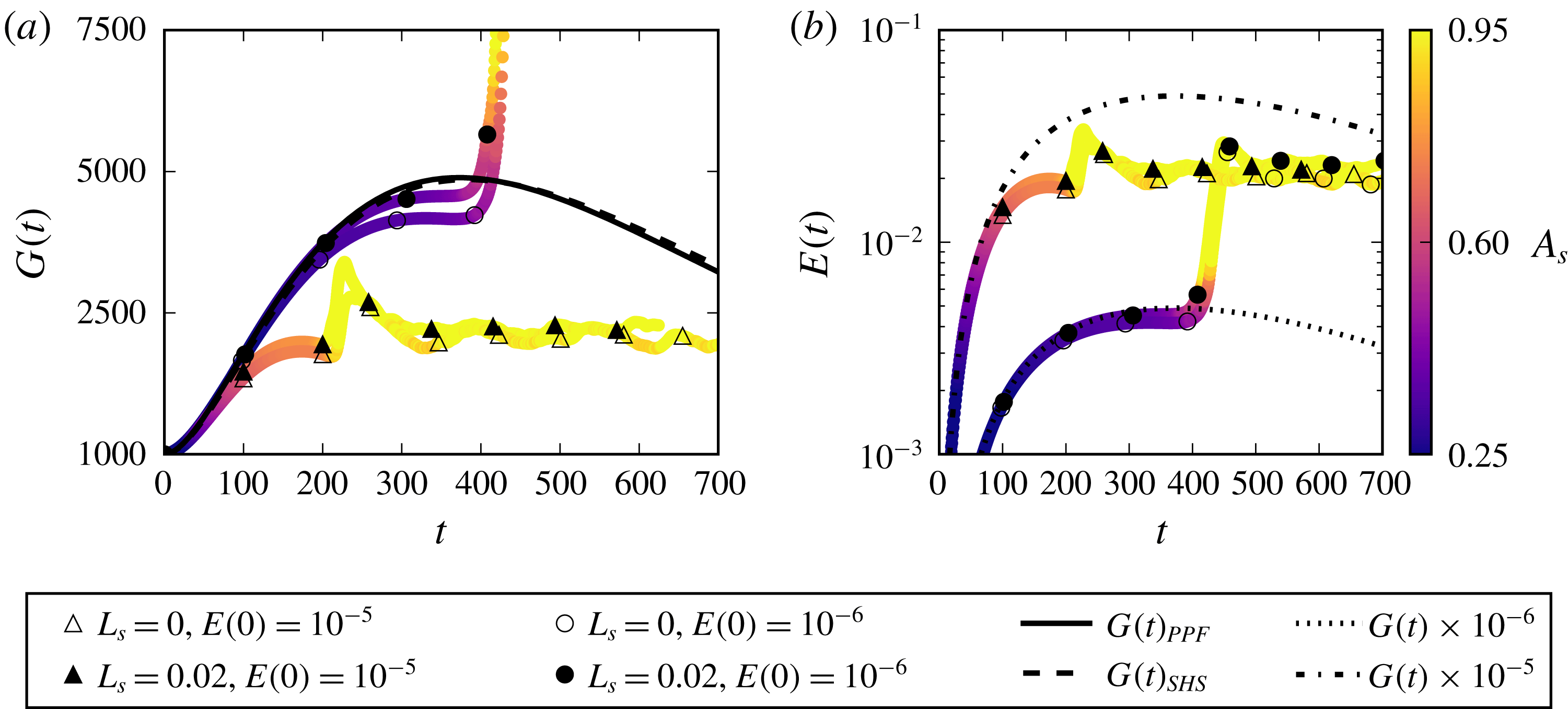
In order to investigate the physical mechanisms affecting transition in the presence of a slippery boundary, we place ourselves in a threshold condition, slightly increasing the initial perturbation intensity up to a value for which transition is triggered even in the
 $L_{s}=0.02$
flow case. This is achieved for a
 $10\,\%$
increase of the perturbation amplitude, namely
 $$\begin{eqnarray}\boldsymbol{U}(t=0)=\boldsymbol{U}_{BF}+1.10(0.03\boldsymbol{u}_{TS_{2D}}\pm 0.001\boldsymbol{u}_{TS_{\pm 3D}}).\end{eqnarray}$$
In the remainder of the paper we will focus on this latter case (3.3), referring to it simply as K-type transition for the sake of simplicity, after having verified that initialising the simulation using (3.2) or (3.3) provides essentially the same results for
 $L_{s}=[0.00,0.01]$
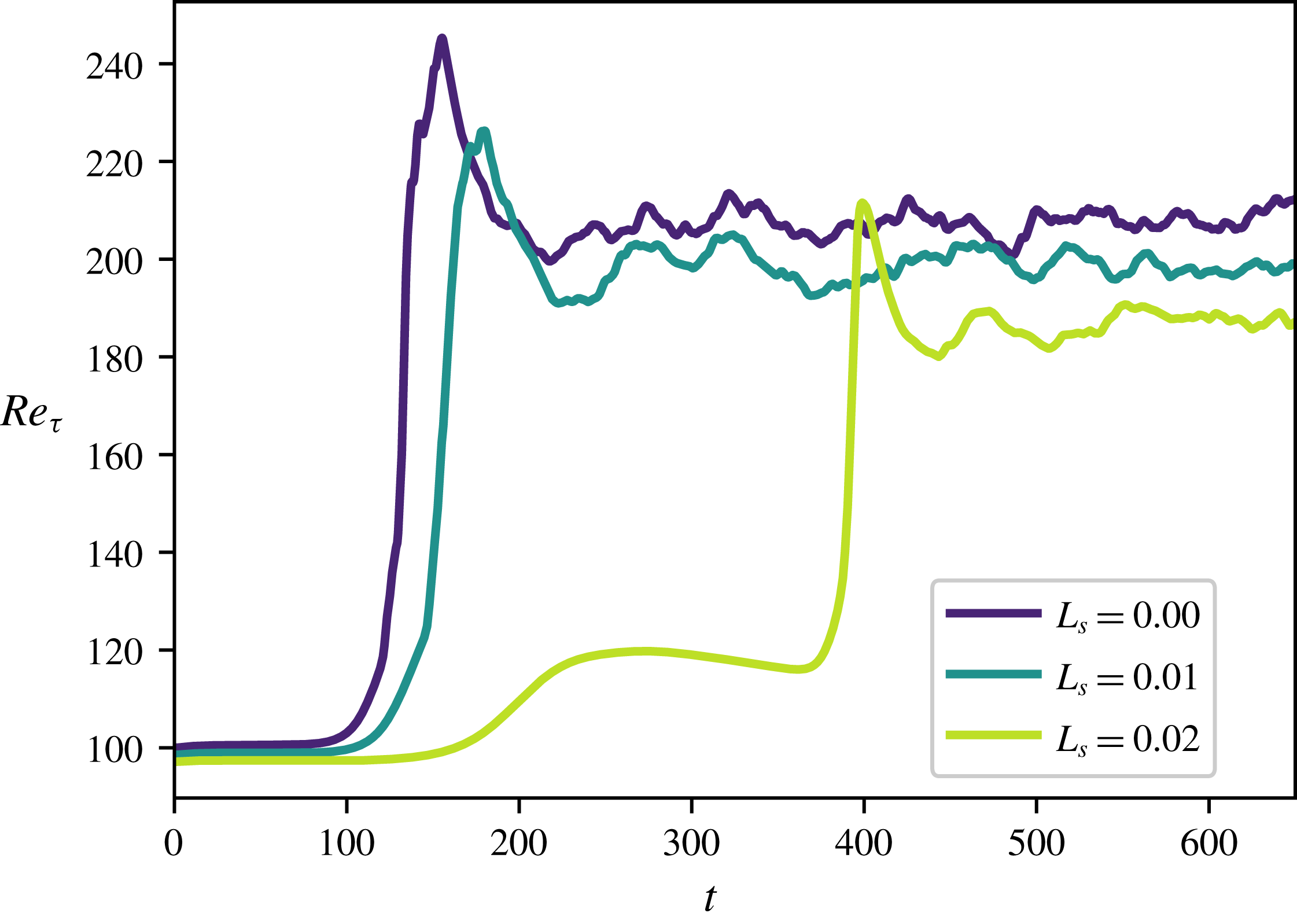
. To detect whether transition has taken place, in figure 6 we provide the evolution of the friction Reynolds number, defined as
 $$\begin{eqnarray}Re_{\unicode[STIX]{x1D70F}}=\sqrt{Re\left|\frac{\unicode[STIX]{x2202}\langle U(\boldsymbol{x},t)\rangle }{\unicode[STIX]{x2202}y}\right|_{wall}},\end{eqnarray}$$
where
 $\langle \cdot \rangle$
represents the spatial average computed on the wall-parallel planes
 $x{-}z$
at a given time
 $t$
and the laminar Reynolds number is set to the constant value
 $Re=5000$
(Zang & Krist Reference Zang and Krist1989). Both the laminar (
 $t<100$
) and turbulent (
 $t>500$
) mean values of
 $Re_{\unicode[STIX]{x1D70F}}$
change with
 $L_{s}$
. The former can be easily derived injecting (2.3) within (3.4)
 $$\begin{eqnarray}Re_{\unicode[STIX]{x1D70F}}=\sqrt{Re\left|\frac{2y}{3L_{s}+1}\right|_{wall}}=\sqrt{\frac{2Re}{(3L_{s}+1)}},\end{eqnarray}$$
while the latter is reduced due to the decreased friction drag. This is a consequence of the fact that we have imposed a constant flow rate. Therefore, we cannot directly compare our results with literature studies of turbulent flows over SHS where
 $Re_{\unicode[STIX]{x1D70F}}$
is kept constant (Min & Kim Reference Min and Kim2004; Seo & Mani Reference Seo and Mani2016).
Looking at the transitional phase, we observe that while
 $Re_{\unicode[STIX]{x1D70F}}$
increases monotonically for
 $L_{s}=[0.00,0.01]$
, this is not the case for
 $L_{s}=0.02$
, where a transient growth of the friction Reynolds number is observed, followed by a saturation and a rapid increase towards the turbulent value. In the following sections we will analyse the coherent structures and associated Fourier modes arising in the different stages of transition with the aim of identifying the instability mechanisms inhibited by the presence of SHS.
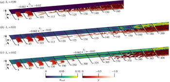
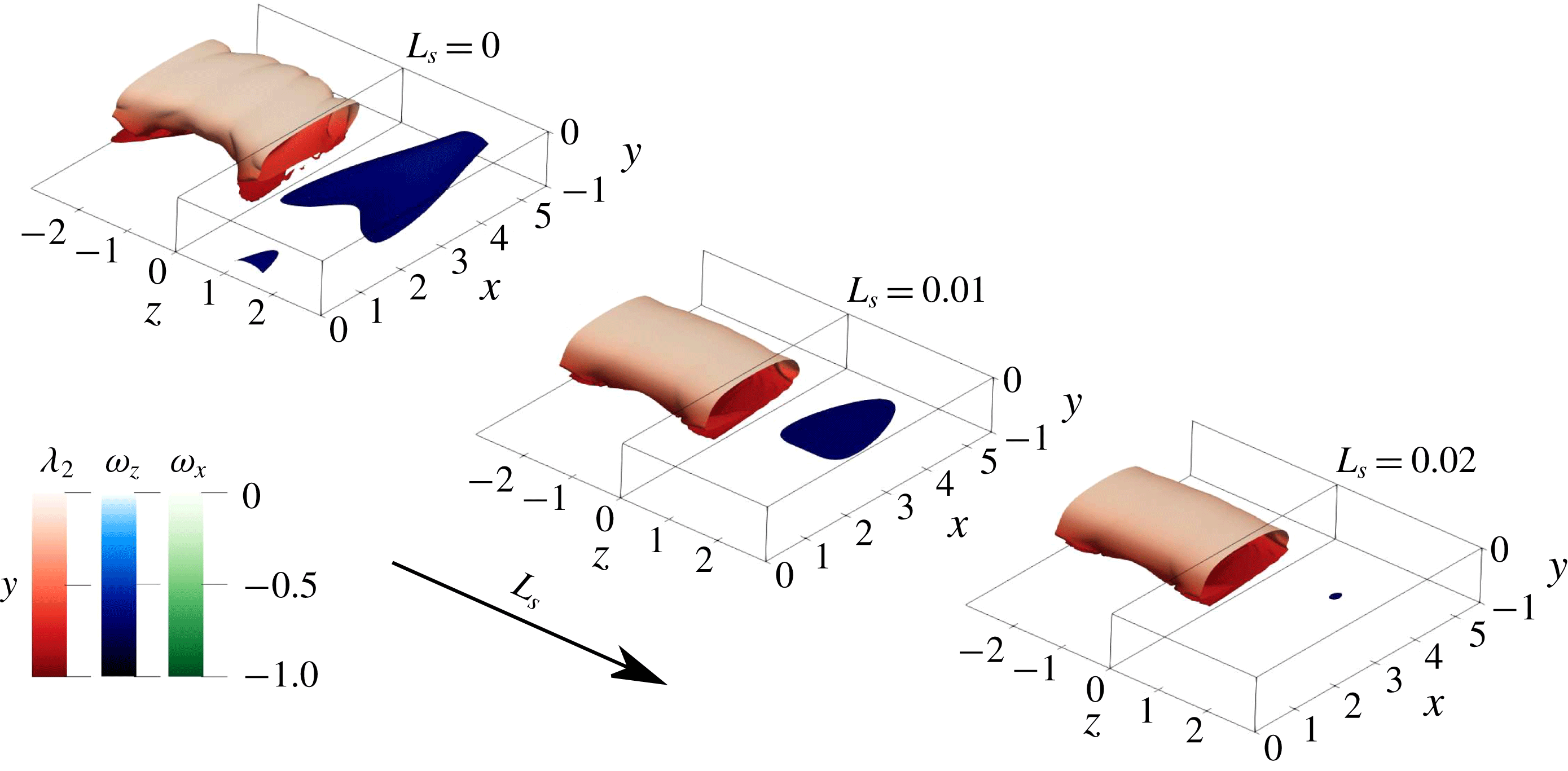
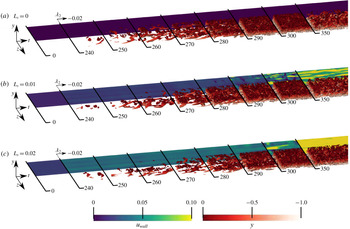
Overview of the K-type transition over superhydrophobic surfaces with different slip lengths. For each slip length, snapshots extracted at different times are placed next to each other in order to provide an overall view of the laminar–turbulent transition process. The time values are reported on the black lines separating the snapshots. The isosurfaces show the
 $\unicode[STIX]{x1D706}_{2}$
criterion, coloured by its distance from the wall, and the isocontours represent the streamwise velocity measured at the lower wall, shifted in the spanwise direction for visualisation purposes. Only the lower half of the channel is shown for the sake of visualisation.

3.2.1 Coherent structures
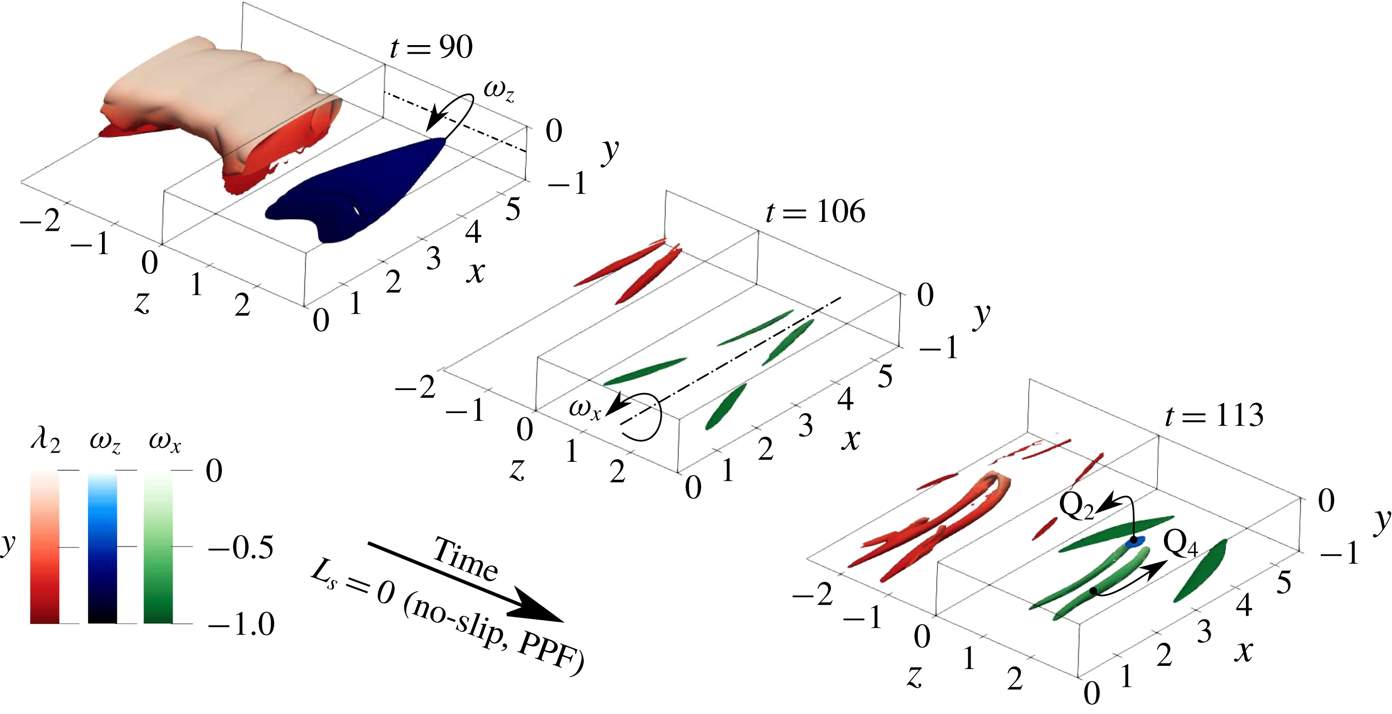
Figure 7 provides snapshots of the flow structures observed during transition to turbulence for the three considered slip lengths. The snapshots are placed next to each other in order to provide an overall view of the transition process; the time at which each snapshot has been extracted is reported in the figure. In figure 7(a) the standard K-type transition scenario is reported for comparison purposes. At first (
 $t\leqslant 80$
) a saturation of the 2-D TS wave is observed, followed by a symmetry breaking in the spanwise direction and a three-dimensionalisation of the perturbation due to secondary instability (
 $t=85$
) (Gilbert & Kleiser Reference Gilbert, Kleiser, Kline and Afgan1990). Then, the presence of strong shear layers promotes the formation of
 $\unicode[STIX]{x1D706}$
-shaped vortices (
 $t=103$
). The roll up of the shear layer connects the downstream side of
 $\unicode[STIX]{x1D706}$
vortices, forming the heads of characteristic hairpin vortices, whereas the legs formed in the upstream part of the
 $\unicode[STIX]{x1D706}$
-vortices are stretched (
 $t=113$
) (Sandham & Kleiser Reference Sandham and Kleiser1992). The late stage of transition (
 $t=125$
) is characterised by the rapid formation of multiple hairpin heads as a succession of sweep-ejection events (Guo et al.
Reference Guo, Borodulin, Kachanov, Pan, Wang, Lian and Wang2010). Finally, at
 $t\geqslant 130$
, breakdown to turbulence is observed.
Figure 7(b) depicts K-type transition over a SHS with
 $L_{s}=0.01$
. Transition appears to be qualitatively similar to the no-slip case in its early stages (
 $t<100$
). Notable differences arise in the late stages, where the
 $\unicode[STIX]{x1D706}$
-vortices weaken and stretch in the streamwise direction (
 $t=125$
). An inhomogeneous streamwise velocity distribution is also observed at the wall
 $(t=120)$
. Hairpin vortices are created at a later time with respect to the no-slip case, showing smaller heads and legs that appear to originate right at the wall, leaving a clear footprint in the slip velocity (
 $t=130$
). Vortical structures such as
 $\unicode[STIX]{x1D706}$
and hairpin vortices persist for a longer temporal range compared to the no-slip case (
 $t\approx 150$
), while the final breakdown to turbulence appears to be qualitatively the same.
Increasing the slip length up to
 $L_{s}=0.02$
, as represented in figure 7(c), produces a drastic change in the transition path. First of all, the spanwise symmetry breaking of the TS waves is considerably delayed in time (
 $t=150$
). Then, the development of
 $\unicode[STIX]{x1D706}$
vortices appears to be inhibited by the slippery walls, leading to a saturation and subsequent slow decrease of the wall shear corresponding to the bump in the
 $Re_{\unicode[STIX]{x1D70F}}$
time series at
 $t=250$
shown in figure 6. At
 $t\approx 300$
, due to flow receptivity (Luchini Reference Luchini2000), the residual perturbations regroup in long, streamwise aligned velocity modulations (streaks), as suggested by the slip velocity distribution at the wall (
 $250<t<275$
), whereas vortices appear almost completely damped. At
 $t\approx 365$
, due to secondary instability of the streaks, new vortical structures arise in the flow, leading to the onset of bypass transition.
3.2.2 Fourier harmonics
With the aim of providing a more quantitative description of how the K-type transition scenario is affected by the use of SHS, we track in time the amplitude of selected Fourier harmonics (Zang & Krist Reference Zang and Krist1989),
 $$\begin{eqnarray}E_{k}(k_{x},k_{z})=\frac{1}{2E_{0}}\int _{-1}^{+1}\left|\hat{\boldsymbol{u}}_{k_{x},k_{z}}(y,t)\right|^{2}\,\text{d}y,\end{eqnarray}$$
where
 $\hat{\boldsymbol{u}}_{k_{x},k_{z}}(y,t)$
is a single component of the Fourier transform of the perturbation velocity field in the streamwise and spanwise directions with wavenumbers
 $k_{x},k_{z}$
, respectively, while
 $E_{0}$
is the kinetic energy of the laminar flow. Following the literature, the wavenumbers of the different Fourier modes will be indicated as multiples of the fundamental wavenumber, the couple
 $(i_{x},i_{z})$
representing the
 $i\text{th}$
multiple of the fundamental streamwise and spanwise wavenumbers,
 $2\unicode[STIX]{x03C0}/L_{x},2\unicode[STIX]{x03C0}/L_{z}$
, respectively. We recall that in this framework the presence of the TS waves
 $u_{TS_{2D}},u_{TS_{\pm 3D}}$
is translated into spikes in the
 $(1,0)$
and
 $(1,\pm 1)$
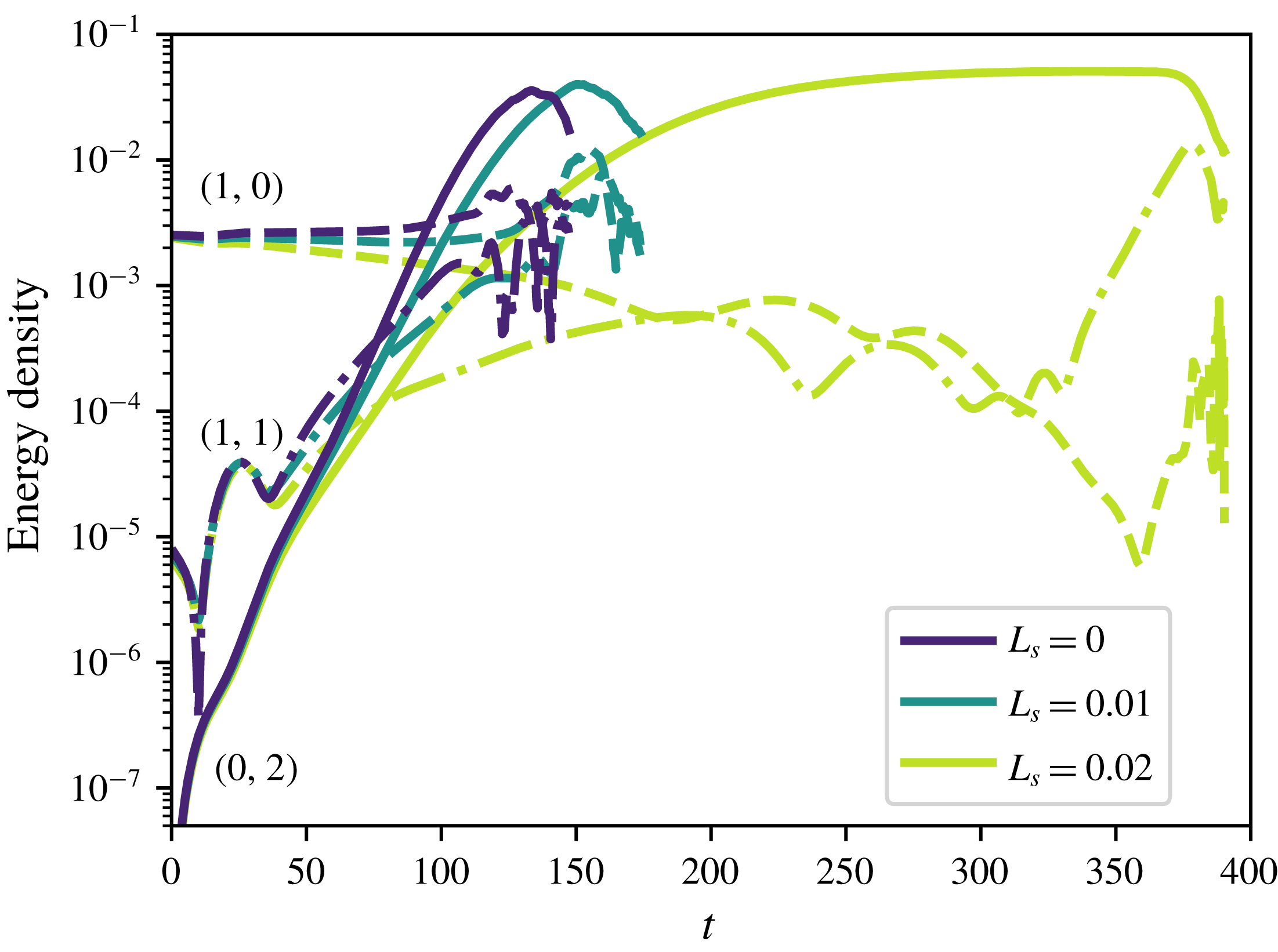
Fourier modes, respectively. The time evolution of the most energetic Fourier modes during the different phases of the K-type transition is provided in figure 8 for the considered values of the slip length. In all cases, despite the fact that energy is initially provided only to the
 $(1,0)$
and
 $(1,\pm 1)$
modes, a streamwise invariant, subharmonic mode
 $(0,2)$
is immediately generated, rapidly increasing in energy. This is a clear sign that, even if the modes initial amplitude is relatively small, nonlinear interactions are already taking place, indicating that predictions based on linear amplification mechanisms are not sufficient to model the transition scenario (Min & Kim Reference Min and Kim2005). For
 $L_{s}=0.00$
and
 $L_{s}=0.01$
the time evolution of the Fourier modes is substantially similar. On the other hand, for the
 $L_{s}=0.02$
case we observe a decrease of the amplitude of the
 $(1,0)$
mode and a much slower increase of
 $(1,1)$
and
 $(0,2)$
modes. At
 $t\approx 200$
, the streamwise-dependent modes begin to decrease in energy whereas mode
 $(0,2)$
saturates for a rather long time range. Thus, for
 $t>200$
the flow is mostly characterised by streamwise-invariant velocity modulations, i.e. streaky structures.
Time evolution of the energy associated with (1, 0), (1, 1) and (0, 2) Fourier modes during K-type transition for different values of
 $L_{s}$
. While the 2-D and 3-D TS waves, respectively identified by modes (1, 0) and (1, 1), evolve in a similar way in all cases, for the
 $L_{s}=0.02$
case streaks ((0, 2) modes) dominate the flow evolution for a large time range, leading to a considerable delay in transition.

3.2.3 Late stages of transition
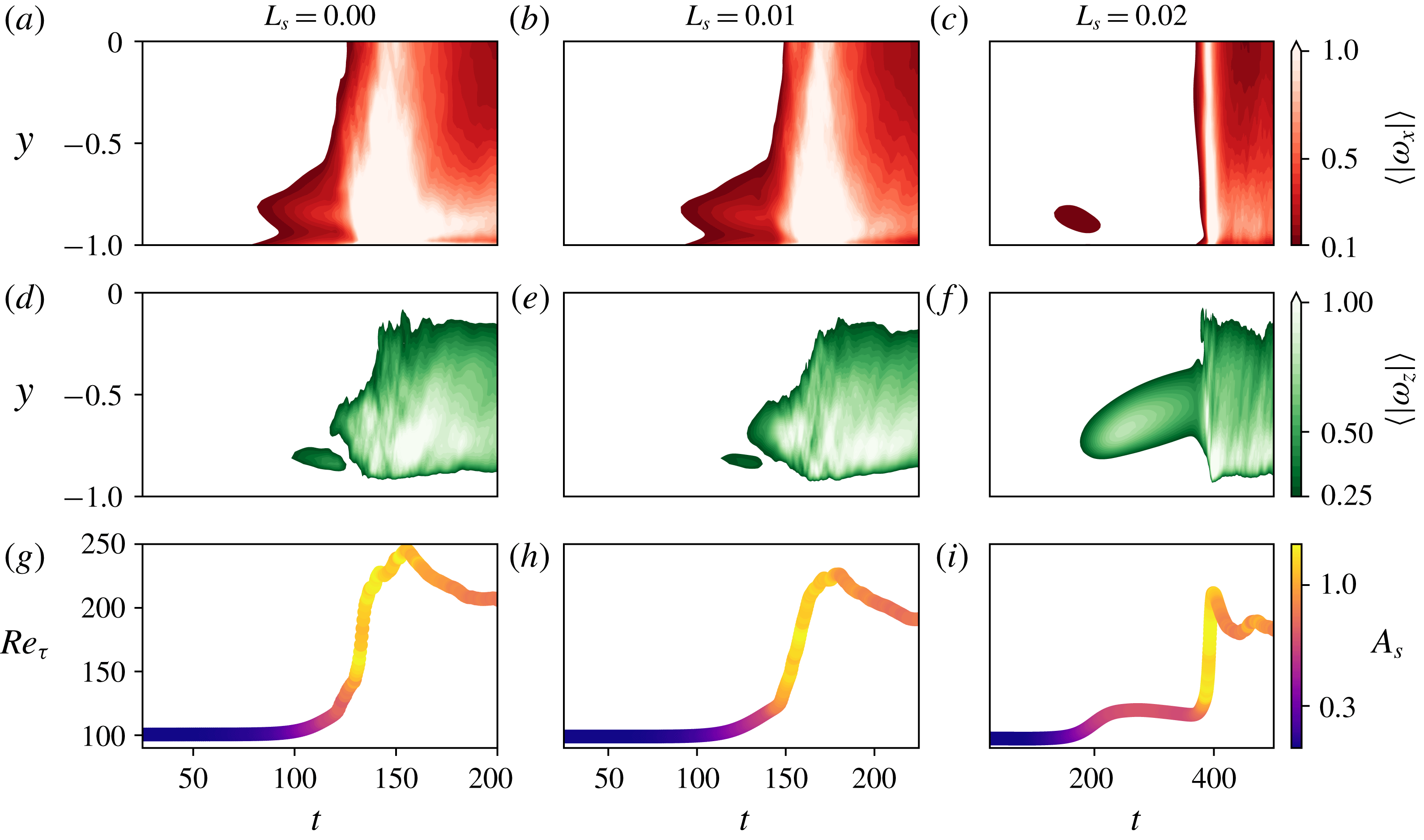
In order to follow the development and eventual disruption of these streaky structures, in figure 9 we provide the time evolution of the streamwise and spanwise vorticities
 $(\unicode[STIX]{x1D714}_{x}=(\unicode[STIX]{x2202}w/\unicode[STIX]{x2202}y)-(\unicode[STIX]{x2202}v/\unicode[STIX]{x2202}z);\unicode[STIX]{x1D714}_{z}=(\unicode[STIX]{x2202}v/\unicode[STIX]{x2202}z)-(\unicode[STIX]{x2202}u/\unicode[STIX]{x2202}y))$
within the channel section, as well as the friction Reynolds number (bottom) coloured by the amplitude of the spanwise modulation, which is defined as
 $$\begin{eqnarray}A_{s}(t)=[\max _{y,z}(\boldsymbol{U}(\boldsymbol{x},t)-\boldsymbol{U}_{b}(\boldsymbol{x},t))-\min _{y,z}(\boldsymbol{U}(\boldsymbol{x},t)-\boldsymbol{U}_{b}(\boldsymbol{x},t))]\end{eqnarray}$$
as proposed by Andersson, Berggren & Henningson (Reference Andersson, Berggren and Henningson1999), Brandt et al. (Reference Brandt, Cossu, Chomaz, Huerre and Henningson2003). Monitoring these quantities in time allows us to identify the hairpin legs and heads, characterised by high values of
 $\unicode[STIX]{x1D714}_{x},\unicode[STIX]{x1D714}_{z}$
, respectively (Zhou et al.
Reference Zhou, Adrian, Balachandar and Kendall1999), as well as the onset of spanwise vortices, associated with peaks of
 $\unicode[STIX]{x1D714}_{z}$
and
 $A_{s}$
(Brandt et al.
Reference Brandt, Cossu, Chomaz, Huerre and Henningson2003). The time evolution of these three quantities is qualitatively and quantitatively similar for the
 $L_{s}=[0.00,0.01]$
cases, as reported in figure 9(a,b,d,e,g,h). In both cases, the formation of
 $\unicode[STIX]{x1D706}$
vortices (localised peak in
 $\unicode[STIX]{x1D714}_{x}$
for
 $t<100$
in figure 9(a,b)) is followed by their evolution into hairpin vortices, as suggested by the
 $\unicode[STIX]{x1D714}_{z}$
spot at
 $t\approx 125$
indicating the rapid development of hairpin heads (see figure 9
d,e). Although this
 $\unicode[STIX]{x1D714}_{z}$
peak is weaker for the
 $L_{s}=0.01$
case, in both cases it is followed by a wall-normal spreading of both vorticity components together with a rapid increase of
 $Re_{\unicode[STIX]{x1D70F}}$
, indicating the breakdown of hairpin vortices and consequent transition to turbulence (Sandham & Kleiser Reference Sandham and Kleiser1992). Figure 9(g,h) is also very similar, although for the slip case the transitional phase is longer and
 $Re_{\unicode[STIX]{x1D70F}}$
is characterised by a smaller value at large time.
This process is radically modified for the largest slip length considered here,
 $L_{s}=0.02$
. Whilst the initial condition has been designed to promote the formation of
 $\unicode[STIX]{x1D706}$
vortices (Sandham & Kleiser Reference Sandham and Kleiser1992),
 $\unicode[STIX]{x1D714}_{x}$
increases only transiently and then drops to very low values, as depicted in figure 9(c). The reduced wall shear restrains the formation of
 $\unicode[STIX]{x1D706}$
vortices, therefore inhibiting the consequent creation of hairpin vortices. Right after the disappearance of the
 $\unicode[STIX]{x1D714}_{x}$
transient peak, at
 $t\approx 200$
,
 $\unicode[STIX]{x1D714}_{z}$
begins to increase, initially close to the wall and then migrating through the channel bulk up to
 $t\approx 400$
(see figure 9
f). In this time range the friction Reynolds number
 $Re_{\unicode[STIX]{x1D70F}}$
increases to a value larger than the laminar but lower than the turbulent mean one and the spanwise modulation amplitude saturates, as shown in figure 9(i). In fact, in this phase streaky structures are created as a response of the flow to the residual perturbations present in the computational domain (Luchini Reference Luchini2000). For
 $180<t<200$
the streaks linearly increase their amplitude (
 $A_{s}$
) due to flow receptivity. Once
 $A_{s}$
reaches a threshold amplitude, nonlinear effects set in (according to Brandt et al. (Reference Brandt, Cossu, Chomaz, Huerre and Henningson2003),
 $A_{s}\approx 26\,\%$
of the free-stream velocity for sinuous instability), and lead to a saturation of both
 $Re_{\unicode[STIX]{x1D70F}}$
and
 $A_{s}$
, while the region of high amplitude
 $\unicode[STIX]{x1D714}_{z}$
departs from the wall. This indicates that the initial ‘linear’ streaks are deformed in the wall-normal direction due to nonlinear effects (Mao et al.
Reference Mao, Zaki, Sherwin and Blackburn2017). Finally, at
 $t>400$
, abrupt secondary instability of these nonlinearly saturated flows occurs and breakdown to turbulence is finally reached.
Streamwise and spanwise vorticities averaged along the homogeneous directions
 $x$
–
 $z$
,
 $\langle \unicode[STIX]{x1D714}_{x}\rangle ,\langle \unicode[STIX]{x1D714}_{z}\rangle$
in (a–c) and (d–f), respectively. Panels (g–i) show the time evolution of the friction Reynolds number
 $Re_{\unicode[STIX]{x1D70F}}$
, coloured by the spanwise deformation amplitude
 $A_{s}$
. Plots are arranged in columns according to the
 $L_{s}$
to which they belong.

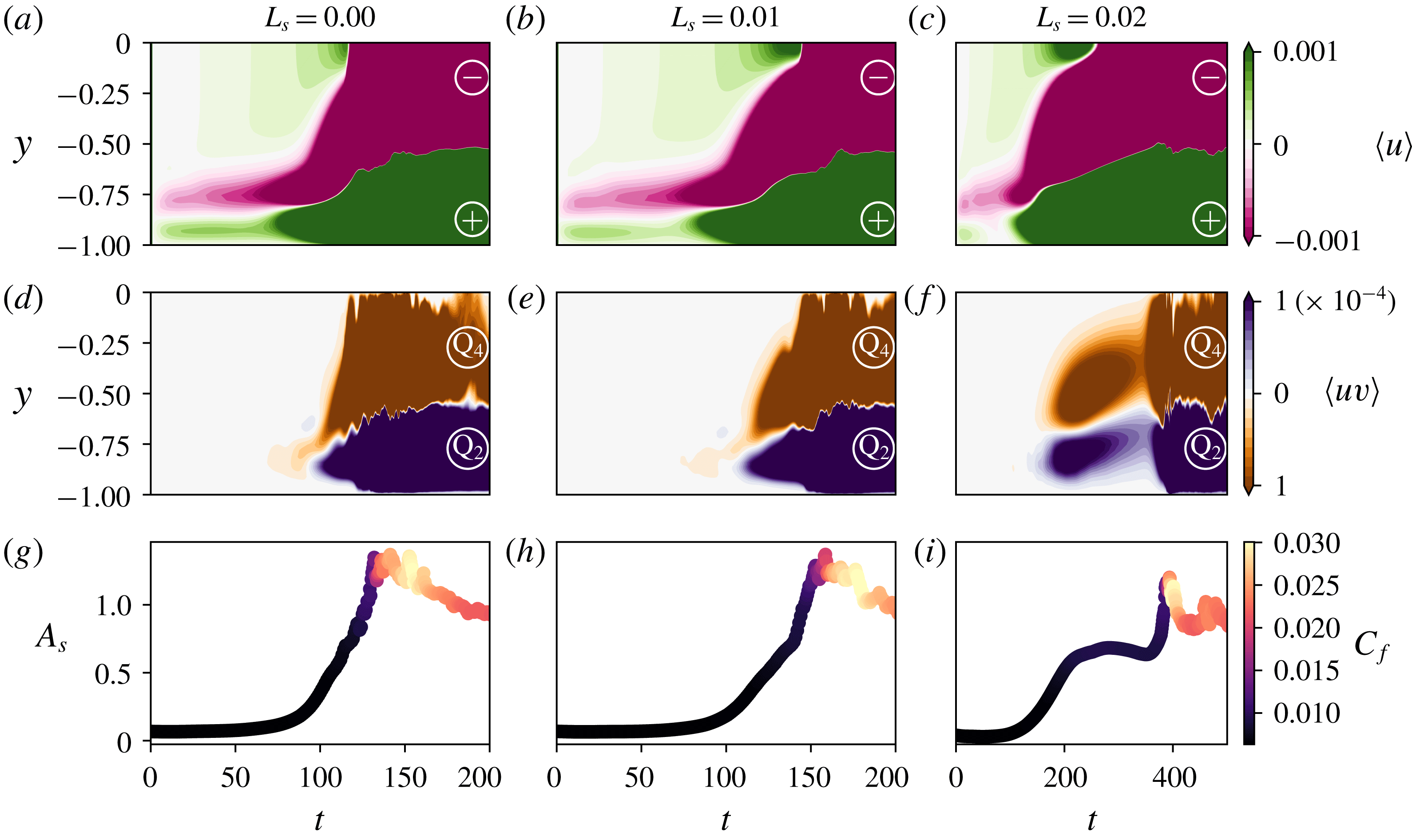
The development of nonlinearly saturated streaks and the consequent creation of hairpin vortices can be further analysed by following the time evolution of the streamwise perturbation and of the
 $uv$
product averaged in the wall-parallel planes as plotted in figure 10 together with the time variation of
 $A_{s}$
coloured by the skin friction coefficient
 $C_{f}$
. The first quantity,
 $\langle u\rangle$
allows us to distinguish linear from nonlinear streaks. In fact, linear high- and low-speed streaks are placed at the same wall-normal positions (Schmid & Henningson Reference Schmid and Henningson2001), thus spanwise averaging cancels out their contribution in the
 $\langle u\rangle$
term. When nonlinearity sets in, since low- (high-) speed streaks migrate upwards (downwards), the quantity
 $\langle u\rangle$
departs from zero. The second quantity,
 $\langle uv\rangle$
, allows us to identify the presence of sweep and ejection events, characterised by large values of
 $\langle uv\rangle$
with
 $u$
and
 $v$
anticorrelated in sign, thus belonging to the Q4 and Q2 quadrants of the
 $u{-}v$
plane, as in Adrian (Reference Adrian2007) and Farano et al. (Reference Farano, Cherubini, Robinet and De Palma2017), although in the present work
 $u,v$
represent fluctuations relative to the base flow (see also Farano et al. (Reference Farano, Cherubini, Robinet and De Palma2015)) and not to the mean flow as in the previously mentioned work. The presence of these events has been indicated in the figure using the Q4 and Q2 nomenclature, as a reminder of the
 $\langle uv\rangle$
velocity quadrant to which they belong. Comparing figures 10(a), 10(b) and 10(c), one can see that, when
 $L_{s}$
increases from
 $0$
to
 $0.02$
, in the time range
 $t=[0,120]$
the quantity
 $\langle u\rangle$
decreases to zero close to the wall, indicating that near-wall linear streaks almost disappear. In the same time range, sweeps and ejections are completely absent in the
 $L_{s}=0.02$
case, whereas for
 $L_{s}=0,0.01$
they occur in the narrow
 $t=[75,100]$
window (compare figures 10
d, e and f). In this time range Q4 (Q2) events occur close to (far from) the wall, as typically observed in the presence of hairpin vortices. On the contrary, at
 $200<t<400$
for the
 $L_{s}=0.02$
case, ejections are observed close to the wall whereas sweeps lay in the outer region (see figure 10
f). This feature can be associated with the onset of nonlinearities saturating the streaks, where the lift-up of the low-speed streaks initially placed in the near-wall region induces Q2 events close to the wall and the downward motion of high-speed streaks produces Q4 events far from the wall. The same wall-normal arrangement of Q2 and Q4 events is observed in all the three cases in the turbulent regime, namely at
 $t>150$
for
 $L_{s}=0,0.01$
and at
 $t>400$
for
 $L_{s}=0.02$
(as indicated by the rapid increase of
 $C_{f}$
at these times), due to the presence of nonlinear streaks in the buffer and viscous layer in the fully turbulent flow (Jiménez Reference Jiménez2013).
(a–c) Contours of the streamwise velocity disturbances averaged onto the
 $x{-}z$
plane,
 $\langle u\rangle$
. (d–f) Contours of the
 $uv$
product measuring Q2 and Q4 events averaged on wall-parallel planes,
 $\langle uv\rangle$
. (g–i) Time evolution of the spanwise amplitude deformation
 $A_{s}$
, coloured by the friction coefficient
 $C_{f}$
. Each column is associated with a given slip length,
 $L_{s}=0.00,0.01,0.02$
from (a–i).

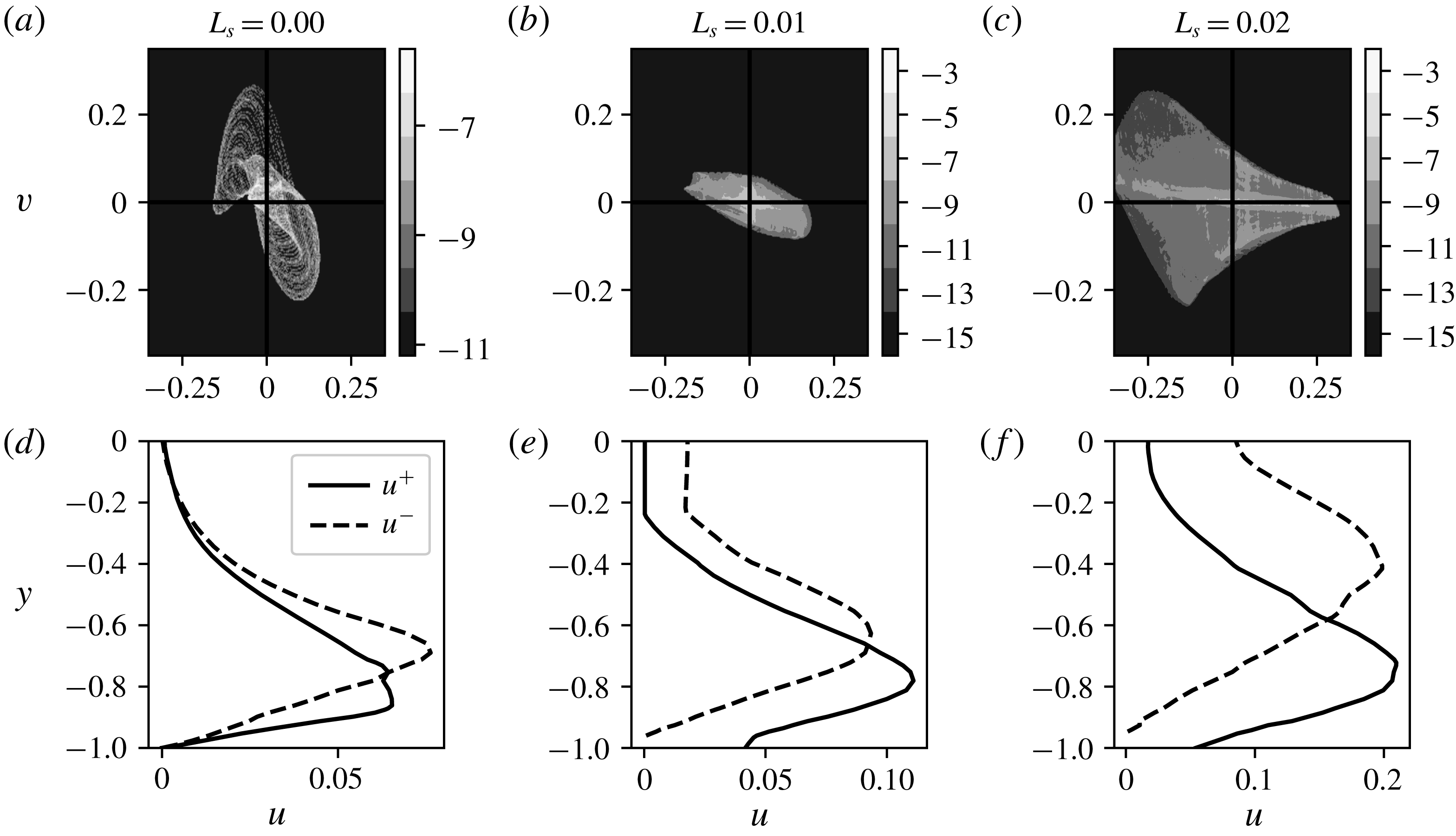
The effect of the slip boundary condition on sweep and ejection events in the nonlinear phase of the transition scenario can be further analysed inspecting the distribution of the
 $u{-}v$
probability density function averaged over the wall-parallel planes in the near-wall region (
 $0<y<1$
), which is provided in figure 11(a–c), together with the wall-normal distribution of the positive/negative streamwise velocity disturbances averaged on
 $x{-}z$
planes (
 $u^{+},u^{-}$
) provided in figure 11(d–f), for different values of
 $L_{s}$
. Sweep and ejection events are attenuated when the slip length is increased from
 $L_{s}=0.0$
to
 $L_{s}=0.01$
(compare figure 11
a with 11
b), whereas the
 $u^{+}$
and
 $u^{-}$
velocity profiles in figure 11(d,e), representing the wake of hairpin legs and heads respectively, remain qualitatively similar. In the case
 $L_{s}=0.02$
, Q4 events are strongly inhibited and the probability density function is mostly dominated by Q2–Q3 events (see figure 11
c), indicating that the flow is characterised by stronger low-speed streaks whose peak value moves upwards in the wall-normal direction (see figure 11
c, bottom), further evidence of the development of nonlinear streaks (Mao et al.
Reference Mao, Zaki, Sherwin and Blackburn2017). Very similar
 $u{-}v$
distribution is found further from the wall (not shown), confirming that the reduced shear succeeds in inhibiting Q4 events everywhere in the flow. These results clearly indicate that for a sufficiently large slip length (
 $L_{s}=0.02$
in the present configuration) the SHS considerably alters the mechanisms leading to the creation of
 $\unicode[STIX]{x1D706}$
and hairpin vortices, inhibiting Q4 events and consequent transition to turbulence. To sum up, K-type transition can be delayed or even completely avoided in the presence of SHS of sufficiently large slip length, for a given amplitude of the imposed initial perturbations.
(a–c) Contours of the logarithm of the probability density function (p.d.f.) of the wall-normal and streamwise velocity disturbances in a
 $u{-}v$
plane (
 $w=0$
) averaged in the wall-parallel planes in the region
 $0<y<1$
. Values of the logarithm of the p.d.f. have been normalised with respect to the total number of points of the computational domain. (d–f) Profiles of the positive/negative (
 $u^{+}/u^{-}$
) streamwise velocity disturbances, averaged on
 $x{-}z$
planes. For each computed
 $L_{s}$
, arranged in columns, we plot the data at time
 $T$
so that the
 $Re_{\unicode[STIX]{x1D70F}}(T)=1.1\cdot Re_{\unicode[STIX]{x1D70F}}(t=0)$
, at the beginning of the nonlinear phase.

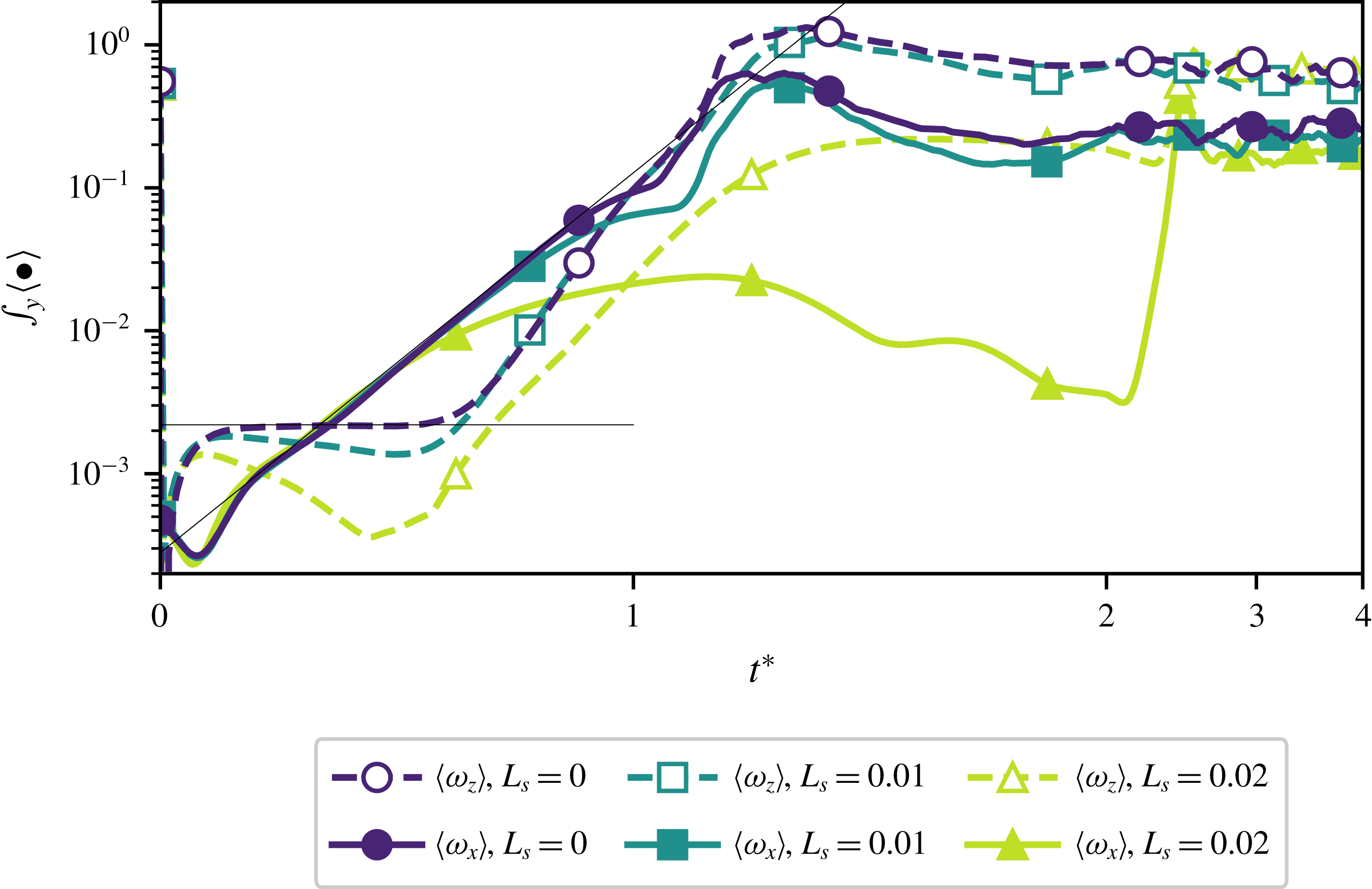
Wall-normal integral of the averaged spanwise and streamwise components of vorticity for different slip lengths. A scaled time
 $t^{\ast }=t/t_{R}$
is used for sake of visualisation, with reference time
 $t_{R}$
conventionally set to the time at which
 $Re_{\unicode[STIX]{x1D70F}}$
reaches
 $1.1Re_{\unicode[STIX]{x1D70F}}(t=0)$
. Straight lines highlight the exponential growth of
 $\unicode[STIX]{x1D714}_{x}$
indicating the vorticity stretching phase (Malm, Schlatter & Sandham Reference Malm, Schlatter and Sandham2011).

3.2.4 How slippery surfaces damp the growth of
 $\unicode[STIX]{x1D6EC}$
vortices

We have shown that a slippery boundary is capable of delaying K-type transition by considerably modifying the coherent structures occurring in the process (Bake, Meyer & Rist Reference Bake, Meyer and Rist2002; Sayadi, Hamman & Moin Reference Sayadi, Hamman and Moin2013). In particular, figure 7 clearly shows that introducing a slip length inhibits the development of hairpin vortices by strongly damping the growth of
 $\unicode[STIX]{x1D6EC}$
vortices. Since during K-type transition
 $\unicode[STIX]{x1D6EC}$
vortices result from the vortex tilting of the spanwise vorticity associated with the initially imposed TS waves (Malm et al.
Reference Malm, Schlatter and Sandham2011), we focus on the effect of the slippery walls on the streamwise and spanwise vorticities. Figure 12 provides the time evolution of the wall-normal averaged values of
 $\langle \unicode[STIX]{x1D714}_{x}\rangle ,\langle \unicode[STIX]{x1D714}_{z}\rangle$
for the three considered slip lengths. For
 $L_{s}=0.00$
we observe an initial increase of
 $\unicode[STIX]{x1D714}_{z}$
due to the presence of TS waves near the walls. After the spanwise vorticity has reached a plateau value,
 $\unicode[STIX]{x1D714}_{x}$
begins to increase exponentially due to vortex tilting (Malm et al.
Reference Malm, Schlatter and Sandham2011), producing
 $\unicode[STIX]{x1D6EC}$
vortices. The vortex tilting phase leading to the creation of
 $\unicode[STIX]{x1D6EC}$
and subsequent hairpin vortices can be visualised in figure 13. Increasing
 $L_{s}$
results in a reduction of
 $\unicode[STIX]{x1D714}_{z}$
right during the vortex tilting phase, with a consequent weaker growth of
 $\unicode[STIX]{x1D714}_{x}$
(see figure 14). This effect can be analysed by evaluating the different terms of the vorticity transport equation, which for an incompressible flow reads
 $$\begin{eqnarray}\frac{\text{D}\unicode[STIX]{x1D74E}}{\text{D}t}=(\unicode[STIX]{x1D74E}\boldsymbol{\cdot }\unicode[STIX]{x1D735})\boldsymbol{u}+\frac{1}{Re}\unicode[STIX]{x1D6FB}^{2}\unicode[STIX]{x1D74E},\end{eqnarray}$$
where
 $\unicode[STIX]{x1D74E}$
is the three-dimensional vorticity vector field. Assuming
 $Re$
to be large enough so that the diffusive term is small (Ye, Schrijer & Scarano Reference Ye, Schrijer and Scarano2018), the temporal evolution of the spanwise vorticity reduces to
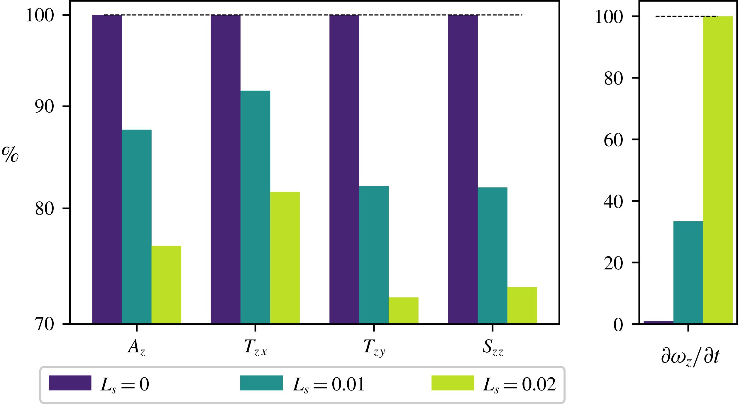
 $$\begin{eqnarray}\frac{\text{D}\unicode[STIX]{x1D714}_{z}}{\text{D}t}\approx \underbrace{-\frac{\unicode[STIX]{x2202}v}{\unicode[STIX]{x2202}z}\frac{\unicode[STIX]{x2202}w}{\unicode[STIX]{x2202}x}}_{T_{zx}}\underbrace{+\frac{\unicode[STIX]{x2202}u}{\unicode[STIX]{x2202}z}\frac{\unicode[STIX]{x2202}w}{\unicode[STIX]{x2202}y}}_{T_{zy}}+\underbrace{\unicode[STIX]{x1D714}_{z}\frac{\unicode[STIX]{x2202}w}{\unicode[STIX]{x2202}z}}_{S_{zz}},\end{eqnarray}$$
where
 $T_{zx},T_{zy}$
and
 $S_{zz}$
represent the vorticity tilting and stretching terms for the spanwise component, respectively. Further development of the latter relation provides the equation which describes the temporal evolution of the spanwise vorticity
 $$\begin{eqnarray}\frac{\unicode[STIX]{x2202}\unicode[STIX]{x1D714}_{z}}{\unicode[STIX]{x2202}t}\approx -\underbrace{\left(u\frac{\unicode[STIX]{x2202}\unicode[STIX]{x1D714}_{z}}{\unicode[STIX]{x2202}x}+v\frac{\unicode[STIX]{x2202}\unicode[STIX]{x1D714}_{z}}{\unicode[STIX]{x2202}y}+w\frac{\unicode[STIX]{x2202}\unicode[STIX]{x1D714}_{z}}{\unicode[STIX]{x2202}z}\right)}_{A_{z}}+\,T_{zx}+T_{zy}+S_{zz}.\end{eqnarray}$$
The volume integral of each term of (3.10) for different values of
 $L_{s}$
, normalised by their value at
 $L_{s}=0$
, is represented in figure 15 for
 $t=23$
. At this time, for
 $L_{s}=0.00$
,
 $\unicode[STIX]{x2202}\unicode[STIX]{x1D714}_{z}/\unicode[STIX]{x2202}t\approx 0$
results from a balance of all terms in (3.10) (although the balance is not exact due to the terms which have been neglected from (3.8)) so that
 $\unicode[STIX]{x1D714}_{z}$
remains constant in time for a large time range. Introducing a slippery boundary, the wall-normal gradients
 $\unicode[STIX]{x2202}(\bullet )/\unicode[STIX]{x2202}y$
(Min & Kim Reference Min and Kim2004) are reduced, inducing a strong decrease of the vortex tilting term
 $T_{zy}=\unicode[STIX]{x2202}u/\unicode[STIX]{x2202}z\cdot \unicode[STIX]{x2202}w/\unicode[STIX]{x2202}y$
. It is important to remark that all terms in (3.10) are affected by the slip length. However, the reduction of the stretching term is indirectly due to the decrease of
 $\unicode[STIX]{x1D714}_{z}$
, rather than to the reduction of the wall-normal shear directly induced by the slippery boundary. Thus, as the slip length is increases,
 $\unicode[STIX]{x2202}\unicode[STIX]{x1D714}_{z}/\unicode[STIX]{x2202}t$
departs from zero due to the imbalance of the advection, tilting and stretching terms in (3.10). This leads to a decrease of the spanwise vorticity and consequently of the vortex-tilting-induced streamwise one, inhibiting the growth of
 $\unicode[STIX]{x1D6EC}$
vortices. Thus, introducing a slippery boundary mildly influences the evolution of the TS spanwise vortices, while strongly affecting the subsequent onset of
 $\unicode[STIX]{x1D6EC}$
vortices by reducing
 $\unicode[STIX]{x1D714}_{z}$
, as clearly shown in figure 14.
Isosurfaces of
 $\unicode[STIX]{x1D706}_{2}$
(red, on the left) and
 $\unicode[STIX]{x1D714}_{z},\unicode[STIX]{x1D714}_{x}$
(blue, green, on the right) during K-type transition over a no-slip (
 $L_{s}=0.00$
) wall at different times indicated in the plot:
 $\unicode[STIX]{x1D706}_{2}=-0.001,\unicode[STIX]{x1D714}_{z}=2.0$
for
 $t=90$
;
 $\unicode[STIX]{x1D706}_{2}=-0.02,\unicode[STIX]{x1D714}_{x}=0.8,\unicode[STIX]{x1D714}_{z}=3.0$
for the other snapshots. Isosurfaces are coloured with their wall-normal location (darker is closer to the wall). PPF, plane Poiseuille flow.

Isosurfaces of
 $\unicode[STIX]{x1D706}_{2}=-0.001$
(red, on the left) and
 $\unicode[STIX]{x1D714}_{z}=1.475,\unicode[STIX]{x1D714}_{x}=1.0$
(blue, green, on the right) at
 $t=90$
during K-type transition over a no-slip wall and for increasing slip lengths. Whilst spanwise vortices arising from the weakly nonlinear interaction of TS waves appear to remain substantially unchanged,
 $\unicode[STIX]{x1D714}_{z}$
is strongly reduced by the introduction of a slippery wall.

Volume integral of the different terms in the spanwise vorticity equation (3.10) for
 $t=23$
and different slip lengths
 $L_{s}$
, normalised with respect to their values measured for
 $L_{s}=0.00$
. On the right-hand side, the
 $\unicode[STIX]{x2202}\unicode[STIX]{x1D714}_{z}/\unicode[STIX]{x2202}t$
term, scaled with respect to its value at
 $L_{s}=0.02$
is shown. The scaling chosen enhances how the evolution of each term of (3.10) changes when wall slip is increased.

4 Transition triggered by non-modal mechanisms
4.1 Optimal perturbations
In subcritical conditions in a noisy environment, streaky perturbations are usually observed prior to transition (Kendall Reference Kendall1998; Saric, Reed & Kerschen Reference Saric, Reed and Kerschen2002; Manneville Reference Manneville2015), since small-amplitude environmental perturbations project in time onto the largest singular value of the linearised Navier–Stokes operator
 $\boldsymbol{L}$
(Luchini Reference Luchini2000), whose associated response corresponds to the optimal perturbation for the considered flow (Farrell Reference Farrell1988). Optimal perturbations are able to induce, by means of non-normal yet linear interaction of eigenmodes of
 $\boldsymbol{L}$
, the maximum possible transient energy growth in a finite time range (Schmid & Henningson Reference Schmid and Henningson2001). This energy growth allows for the development of nonlinear interactions, leading the flow to transition. To study the effect of the SHS on this optimal transition scenario, we impose as initial condition
 $\boldsymbol{U}(\boldsymbol{x},t=0)=\boldsymbol{U}_{b}(\boldsymbol{x})+\unicode[STIX]{x1D716}\boldsymbol{u}_{0}^{Opt}(\boldsymbol{x})$
, where
 $\unicode[STIX]{x1D716}\boldsymbol{u}_{0}^{Opt}(\boldsymbol{x})$
is the initial optimal perturbation computed in the chosen flow conditions and
 $\unicode[STIX]{x1D716}$
is a given amplitude, which has to be set sufficiently high to trigger nonlinear effects and consequently lead to transition (Reshotko Reference Reshotko2001). Being derived from linearised equations, the optimal perturbation can be freely scaled so to match an arbitrarily imposed energy level. If the initial perturbation energy is set to a very low value, the initial perturbation, composed of streamwise vortices, linearly evolves in time, creating optimal streaks which asymptotically fade away, as predicted by the linear theory. Increasing the initial energy level to
 $E(0)=10^{-6}$
, as shown in figure 16 for the no-slip case, after an initial linear growth phase (
 $0<t<200$
), the streaks saturate nonlinearly (see the inset at the panel c) to an amplitude
 $A_{s}$
. As soon as this amplitude overcomes a critical threshold (Brandt et al.
Reference Brandt, Cossu, Chomaz, Huerre and Henningson2003) secondary instabilities of the nonlinearly saturated optimal streaks set in (
 $t\approx 400$
), immediately followed by breakdown to turbulence. Further increasing the initial energy to
 $E(0)=10^{-5}$
leads to a more rapid departure from the linearly predicted energy growth curve due to the onset of nonlinearities already at very small times, resulting in a different saturation energy threshold. Nonlinearly saturated streaks, strongly deformed with respect to the linear optimal solution, as shown in the top right inset, are formed already at
 $t\approx 150$
and due to secondary instability, breakdown to turbulence is reached already at
 $t\approx 200$
.
(a) Time evolution of the kinetic energy density of the velocity perturbation during laminar–turbulent transitions triggered by linear optimal perturbations, for a no-slip wall (
 $L_{s}=0.00$
) and for two prescribed values of the initial energy,
 $E(t=0)=10^{-6}$
and
 $E(t=0)=10^{-5}$
(thick solid lines coloured by the amplitude of spanwise modulation
 $A_{s}$
, as defined in equation 3.7). The dashed lines indicate the energy growth as predicted by the linear theory for the two imposed initial energy levels. (b) Isocontours of the streamwise velocity perturbation in a
 $z{-}y$
plane for the case with
 $E(t=0)=10^{-6}$
at
 $t=150$
showing the highly deformed nonlinearly saturated streaks. (c) Isocontours of the streamwise velocity perturbation in a
 $z{-}y$
plane for the case with
 $E(t=0)=10^{-5}$
at
 $t=380$
. In both (b) and (c), the velocity field is invariant in the streamwise direction, therefore any
 $x$
-normal plane will provide the same data.

Introducing a slippery boundary does not modify this scenario, as depicted in figure 17. For the smallest considered energy level, the growth rate curves for the cases
 $L_{s}=0.00,0.02$
are very close to each other, although a slightly larger energy gain is reached in the slippery case. The same effect is observed for the largest energy level considered here, where the case at
 $L_{s}=0.02$
appears to follow more closely the linear evolution of
 $G(t)$
with respect to the no-slip one. This is probably due to the fact that in the no-slip case a slightly larger energy growth is predicted by the linear theory at small times (compare the solid with the dashed black lines in the left frame), resulting in a more rapid onset of nonlinear effects which translates into an earlier and more pronounced deviation from the linear energy growth curve. However, in both cases, secondary instability is reached practically at the same time, since the energy level reached in the saturation phase (see the right frame of figure 17) and the shape of the nonlinearly saturated streaks (see figure 18) appear to be almost independent on the imposed slip length. The fact that, differently from the K-type one, the optimal transition scenario is virtually unaffected by the introduction of a slip length can be explained by the fact that the optimal perturbations are localised in the bulk of the channel, as opposed to TS waves which are placed close to the wall. Since SHS act by modifying the flow shear near the wall, it appears clear why optimal streaks are unaffected by this boundary modification even when nonlinearities kick in, as depicted in figure 18.
Influence of SHS on subcritical transition at
 $Re=5000$
triggered by linear optimal perturbations. Both panels represent the same dataset, but with different scales. In (a) the energy gain evolution is plotted to highlight the initial linear phases, whereas (b) provides the energy, for two initial energy levels and two slip lengths, as indicated in the legend. The dashed lines indicate the energy growth as predicted by the linear theory for the two imposed initial energy levels.

Streamwise velocity perturbation measured at
 $t=150$
in a DNS initialised with the optimal perturbation having initial energy
 $E(t)=10^{-5}$
for different slip lengths. The nonlinear streaks observed in the no-slip case (
 $L_{s}=0.0$
, figure 16
c) match those developing on a slippery surface with
 $L_{s}=0.02$
.

4.2 Uncontrolled transition
In this section we aim to study how uncontrolled transition, namely that naturally occurring in a noisy environment in subcritical conditions, is affected by the presence of superhydrophobic walls. Uncontrolled transition in a channel flow can be triggered using random noise, a random superposition of Stokes modes or, as recently proposed in Picella et al. (Reference Picella, Bucci, Cherubini and Robinet2019), using an ad hoc volume forcing, constructed by a superposition of optimal forcing functions, able to trigger a large-amplitude response in the flow as a consequence of receptivity. The latter technique, which we refer to as F-type transition, has been chosen here to study the effect of SHS on laminar–turbulent uncontrolled transition. Following the procedure described by Picella et al. (Reference Picella, Bucci, Cherubini and Robinet2019), we have constructed a noisy volume forcing using a basis of harmonic disturbances that maximise (within a linear framework) the flow response for different given frequencies (Schmid & Henningson Reference Schmid and Henningson2001). The synthetic noisy volume forcing is then constructed as a linear composition of these optimal volume forcings issued from resolvent analysis, suitably weighted in order to respect a chosen energy spectrum. In the present case the noisy forcing has been constructed using a basis of
 $N_{\unicode[STIX]{x1D714}}\times N_{\unicode[STIX]{x1D6FC}}\times N_{\unicode[STIX]{x1D6FD}}=64\times 4\times 4$
optimal forcing functions (referring to the number of temporal, streamwise and spanwise wavenumbers taken into account for constructing it), with an initial turbulence intensity set to
 $0.35\,\%$
of the reference velocity
 $U_{r}$
. In figure 19 we show the impact of SHS on uncontrolled transition. Increasing
 $L_{s}$
is totally ineffective in delaying the onset of turbulence, as shown by the evolution of the friction Reynolds number during F-type transition (figure 19
a). As explained by Picella et al. (Reference Picella, Bucci, Cherubini and Robinet2019) in the framework of a channel flow with no-slip walls, the imposed volume forcing acts similarly to a noisy environmental disturbance, promoting the development of streaks as a response of the flow to external disturbances (Jacobs & Durbin Reference Jacobs and Durbin2001; Schmid & Henningson Reference Schmid and Henningson2001; Brandt, Schlatter & Henningson Reference Brandt, Schlatter and Henningson2004). As previously shown in figure 17, streaks are mildly affected by a slippery boundary condition, being localised far from the walls. This is confirmed by figure 19(b), where the time evolution of the Fourier modes
 $(0,1)$
,
 $(1,1)$
and
 $(0,2)$
is provided, clearly showing the onset of streaks (i.e.
 $(0,1)$
) and
 $(0,2)$
modes) from a noisy disturbance due to receptivity, followed by their nonlinear saturation as well as their final breakdown. Practically no difference can be noticed between the modes’ evolution for the considered three slip lengths. The time evolution of the coherent structures associated with uncontrolled transition is provided in figure 20. The flow evolution appears very similar for the three slip lengths considered, except for the non-zero velocities measured at the wall in the SHS cases, which have practically no influence on the mechanisms leading to transition. Thus, we can conclude that uncontrolled transition cannot be effectively controlled by SHS, at least for the considered values of the slip length. In fact, similarly to the optimal transition scenario, uncontrolled transition mostly relies on the onset and instability of streamwise streaks, which are both intrinsically inviscid mechanisms not strongly affected by the presence of a slippery wall.
Time evolution of the friction Reynolds number
 $Re_{\unicode[STIX]{x1D70F}}$
and of the energy of three selected Fourier modes for channel flows with different slip lengths undergoing F-type transition. The process is completely unaffected by the increase of the slip length
 $L_{s}$
.

Overview of F-type transition over superhydrophobic surfaces. As in figure 7, snapshots depict the isosurfaces of the
 $\unicode[STIX]{x1D706}_{2}$
criterion and streamwise velocity at the wall for different values of the slip length
 $L_{s}$
. This uncontrolled scenario, characterised by the onset of streaky velocity perturbations occurring in the flow bulk, appears to be completely unaffected by the introduction of a slippery boundary.

5 Summary and conclusions
In this paper we investigate the influence of a slippery wall modelling the behaviour of a superhydrophobic surface on different laminar–turbulent transition processes, in order to evaluate their effectiveness as passive devices for flow control in transitional conditions. Following Min & Kim (Reference Min and Kim2005), we have focused on the channel flow configuration where the superhydrophobic surfaces have been modelled by flat, spatially homogeneous and isotropic slippery boundaries, which reproduce sufficiently well the dynamics of the flow on superhydrophobic surfaces in wetting-stable conditions. We have performed a wide range of direct numerical simulations showing that transition delay is not only dependent on the intrinsic slip length of a certain superhydrophobic surface, but also strongly depends on the specific transition scenario one aims at controlling. Our investigation has revealed that a slippery wall can effectively control transition scenarios dominated by near-wall perturbations, i.e. Tollmien–Schlichting waves such as those naturally arising in the flow in supercritical conditions or those occurring during K-type transition in subcritical conditions. In this framework, superhydrophobic surfaces alter the development of
 $\unicode[STIX]{x1D706}$
vortices, since the reduced wall-normal velocity gradient inhibits their formation out of the initial Tollmien–Schlichting waves. In turn, this inhibits the formation of hairpin vortices altering the succession of sweep and ejection events, thus provoking relaminarisation or a large delay in the transition time. On the other hand, our analyses indicate that superhydrophobic surfaces are ineffective in controlling transition initiated by linear optimal perturbations, or even uncontrolled transition, namely that occurring in noisy environments in subcritical conditions, where the seeds of transition (namely, streamwise vortices and streaks) are localised in the bulk of the flow, far from the bounding walls. Superhydrophobic surfaces can thus be considered effective in delaying or avoiding transition only in low-noise environments, where transition is triggered mostly by modal mechanisms, but not in noisy ones, where non-modal mechanisms govern the transition scenario.
It remains to be verified whether a more accurate modelling of the superhydrophobic surface might lead to different results. The homogeneous slip condition can be replaced first with a patterned slip/no-slip boundary condition on a flat wall to investigate the effects of this condition on laminar–turbulent transition. Eventually, also the dynamics of the deformable gas/liquid interfaces might be taken into account, as already done by Seo & Mani (Reference Seo and Mani2018) for a turbulent channel flow. Increasing the model accuracy may result in further modifications of the transitional phase, and thus requires further investigation.
Acknowledgements
This work was granted access to the HPC resources of IDRIS, TGCC and CINES under the allocation A0052A06362 made by GENCI (Grand Equipement National de Calcul Intensif). The authors acknowledge the support of the French Agence Nationale de la Recherche (ANR) under grant DETAIL (ANR-15-CE29-0008-01).
Supplementary materials
Supplementary materials are available at https://doi.org/10.1017/jfm.2019.740.
Appendix. Numerical validation
Direct numerical simulations have been validated comparing our results with those provided by Min & Kim (Reference Min and Kim2004) on a fully developed turbulent flow over a superhydrophobic surface. Figure 21(a) depicts the statistics obtained with our code in the turbulent regime. To converge the statistics, the simulations have been run for
 $t\approx 1000$
time units after the onset of a turbulent state. Transition has been triggered following the K-type scenario. The mean velocity profiles
 $U^{+}$
slightly deviate from the reference ones when the slip length is increased. This behaviour is due the fact that our statistically converged states result from laminar–turbulent transition of a channel where we have imposed a constant flow rate for different values of the slip length, instead of a constant mean value of
 $Re_{\unicode[STIX]{x1D70F}}$
in the turbulent regime, as done by Min & Kim (Reference Min and Kim2004). As a consequence, in our numerical configuration the mean friction Reynolds number in the fully developed turbulent regime reduces when the slip length
 $L_{s}$
is increased, since the shear at the wall decreases. To allow for a more direct comparison with the Min & Kim (Reference Min and Kim2004) results we make use of the shifted-turbulent boundary layer model first proposed by Fukagata et al. (Reference Fukagata, Kasagi and Koumoutsakos2006). Using equation (6) from Seo & Mani (Reference Seo and Mani2016) we obtain the profiles in figure 21(b), which compare well with those obtained by DNS. As a further validation we show the Reynolds stresses in figure 22. Our results match the values computed by Schlatter (Reference Schlatter2005) for a no-slip boundary at
 $Re_{\unicode[STIX]{x1D70F}}\approx 210$
, while increasing the
 $L_{s}$
we obtain the same behaviour prescribed by Min & Kim (Reference Min and Kim2004) for a lower friction Reynolds number. This validates our approach, further confirming that the fully turbulent state is independent of the transition route.
(a) Mean velocity profiles compared with the ones obtained for
 $Re_{\unicode[STIX]{x1D70F}}=180$
by Min & Kim (Reference Min and Kim2004). The slight discrepancy between the results derives from the fact that our turbulent states arise from transition made at a constant flow rate. (b) Same mean velocity profiles as in (a), compared with the shifted-turbulent boundary layer model (Fukagata et al.
Reference Fukagata, Kasagi and Koumoutsakos2006), for the different values of
 $Re_{\unicode[STIX]{x1D70F}}$
.

Reynolds stresses in wall scaling for different
 $L_{s}$
. From top to bottom
 $\langle uu\rangle ^{1/2}/u_{\unicode[STIX]{x1D70F}}$
,
 $\langle ww\rangle ^{1/2}/u_{\unicode[STIX]{x1D70F}}$
,
 $\langle vv\rangle ^{1/2}/u_{\unicode[STIX]{x1D70F}}$
,
 $\langle uv\rangle /u_{\unicode[STIX]{x1D70F}}^{2}$
. Open circles represent the values computed for
 $L_{s}=0.0$
(no-slip wall) by Schlatter (Reference Schlatter2005) at
 $Re_{\unicode[STIX]{x1D70F}}\approx 210$
.