





Nomenclature
- ASTM
-
American Society for Testing and Materials
- ASK
-
available seat kilometers
- ATAG
-
Air Transport Action Group
- AtJ
-
alcohol to jet
- CAGR
-
compound annual growth rate
- CAPEX
-
capital expenditure
- CCS
-
carbon capture and storage
- CO2
-
carbon dioxide
- CO2-eq
-
carbon dioxide equivalent
- CORSIA
-
Carbon Offsetting and Reduction Scheme for International Aviation
- DOC
-
direct operating cost
- E
-
energy
- e
-
Emissions
- ERF
-
effective radiative forcing
- FEED
-
feedstock cost
- FOG
-
fats oils and greases
- FT
-
Fischer Tropsch
- Gt
-
gigatonnes
- GWP
-
global warming potential
- HEFA
-
hydroprocessed esters and fatty acids
- IATA
-
International Air Transport Association
- ICAO
-
International Civil Aviation Organization
- IPCC
-
Intergovernmental Panel on Climate Change
- kWh
-
kilowatt hour
- km
-
kilometre
- LHV
-
lower heating value
- MFSP
-
minimum fuel selling price
- MSW
-
municipal solid waste
- MJ
-
megajoule
- NOx
-
nitrogen oxides
- OPEX
-
operating expenditure
- RF
-
radiative forcing
- RPK
-
revenue passenger kilometres
- RQL
-
rich-burn quick-quench lean-burn
- SAF
-
sustainable aviation fuel
- SFC
-
specific fuel consumption
- SOx
-
sulphur oxides
- TCRE
-
transient climate response to cumulative carbon emissions
- Tg
-
teragram
- TRL
-
technology readiness levels
1.0 Introduction
1.1 Background and motivation
Aviation has sustained long-term global growth since its inception, doubling approximately every 15 years [1], and reaching 35.3 million flights and 4.4 billion passengers in 2023, generating 8.17 trillion revenue passenger kilometre (RPK) [2]. While this growth supports global mobility and economic development, it intensifies aviation’s environmental footprint. Currently, aviation contributes 2–3% of global CO2 emissions; however, when including non-CO2 impacts, contrails, nitrogen oxides (NOx), sulphur oxides (SOx) and water vapour, its total effective radiative forcing (ERF) increases to nearly 5% of anthropogenic warming [Reference Lee3]. Although the Carbon Offsetting and Reduction Scheme for International Aviation (CORSIA) initially sought carbon-neutral growth from 2020, the global target has now shifted toward achieving net-zero CO2 emissions by 2050. Meeting this objective necessitates deep technological transitions, alternative energy carriers, operational optimisation and large-scale infrastructure deployment.
Despite extensive works on sustainable aviation fuels (SAF), hydrogen and electrification individually, comparatively fewer works evaluate them in an integrated framework across short-, medium- and long-range operations while simultaneously accounting for CO2, non-CO2 effects, energy efficiency, cost implications and compatibility with current operations. A study conducted by Dray et al. [Reference Dray, Schäfer, Grobler, Falter, Allroggen, Stettler and Barrett4], addresses a similar challenge; however, it focuses primarily on specific low-carbon fuel options and does not consider an integrated pathway that combines multiple decarbonisation strategies, such as electrification and carbon offsetting, within a unified framework. Addressing this gap motivates the present study, which also evaluates an additional `baseline continuation’ pathway, wherein aviation remains reliant on Jet A1 and achieves emissions reductions exclusively through operational improvements and carbon offset mechanisms.
1.2 Emerging pathways for sustainable aviation
SAFs represent the most mature and immediately deployable decarbonisation pathway due to their drop-in compatibility with existing aircraft and fuel infrastructure. When produced from sustainable feedstocks, biofuels and electrofuels can deliver lifecycle CO2 reductions of approximately 60–90%, depending on production pathways and energy sources [Reference Detsios5, Reference De Jong6]. Despite differing maturity levels and resource demands, SAFs remain the only near-term solution compatible with the current fleet and are certified for blends of up to 50% with Jet A1 under American Society for Testing and Materials (ASTM) D7566 and D1655 standards.
Hydrogen propulsion eliminates tank-to-wake CO2 emissions relative to kerosene [Reference Yusaf7], although non-CO2 effects such as NOx formation and contrail induced radiative forcing (RF) persist. Deployment is constrained by challenges in hydrogen production, storage, airframe integration and low NOx combustion, making large-scale adoption dependent on further technological advances [Reference Yusaf7, Reference Cecere, Giacomazzi, Di Nardo and Calchetti8].
Electrification enables zero-emission propulsion for short-range aircraft, with hybrid electric concepts offering fuel-burn reductions on regional missions. However, limitations in battery energy density, conversion efficiency and thermal management limit applicability beyond these ranges [Reference Gong9].
A continuation pathway based on conventional kerosene mitigates emissions through operational improvements and large-scale carbon offsetting. While this approach limits near-term disruption, it remains fundamentally constrained by ongoing fossil fuel combustion and its associated CO2 and non-CO2 climate impacts.
1.3 Scope and contribution of the present study
Collectively, these pathways illustrate the breadth of technological, operational and energy system transformations required for aviation to align with long-term climate objectives. Each pathway offers distinct strengths yet remains constrained by feedstock availability, energy demand, technology readiness, infrastructure requirements and cost [Reference Dray, Schäfer, Grobler, Falter, Allroggen, Stettler and Barrett4]. No single solution can independently deliver net-zero aviation, making a comparative evaluation essential to understand their respective contributions, limitations and interactions across mission ranges.
Accordingly, the present study employs the AeroMAPS framework to assess these pathways in a unified manner, quantifying their CO2 and non-CO2 impacts, energy performance and operational feasibility across short-, medium- and long-range operations. By integrating both technological and operational scenarios, this work establishes a basis for identifying credible decarbonisation trajectories for the global aviation sector.
2.0 Methodology
2.1 Overview of the modelling framework
The analysis employs AeroMAPS, a long-term aviation modelling framework developed at ISAE-SUPAERO by Planès, Delbecq and Salgas [Reference Planès, Delbecq and Salgas10]. AeroMAPS is designed to evaluate the environmental and operational implications of future aviation decarbonisation pathways by simulating aircraft performance, emissions and fleet evolution under a range of technology and policy scenarios. The tool estimates fuel consumption and energy use using representative aircraft performance assumptions and technology scenarios, differentiated across short-, medium-, and long-range mission profiles, rather than simulating detailed aircraft and engine flight operations, and combines these with lifecycle emissions inventories to enable consistent estimation of CO2 and non-CO2 climate effects [Reference Planès, Delbecq and Salgas10].
Multiple propulsion and fuel configurations, including Jet A1, sustainable aviation fuel (SAF) blends, hydrogen combustion, electric and hybrid electric technologies, can be applied across short-, medium- and long-range aircraft. This segmentation captures differences in mission profiles, energy requirements, fuel-burn characteristics and technology readiness, ensuring that each pathway is assessed within the operational contexts for which it is most feasible. Moreover, operational parameters such as load factor evolution, aircraft efficiency improvements and fleet renewal dynamics are incorporated, alongside measures to mitigate non-CO2 effects, enabling an evaluation of both technological and operational mitigation strategies.
2.2 Fleet and mission definition
The air transport system is structured into three mission categories, short (
 $\lt $
1500 km), medium (1500–4000 km) and long range (
 $\gt $
4000 km), reflecting differences in aircraft architecture, operational profiles and energy requirements [Reference Planès, Delbecq and Salgas10]. Representative aircraft are selected for each category, and a calibrated mix of older and newer aircraft is applied to reproduce observed historical trends in fleet energy intensity [Reference Planès, Delbecq and Salgas10].
Air transport in AeroMAPS is represented through three interconnected components: air traffic, aircraft fleet and operations and aircraft energy linked through an adapted Kaya identity that expresses CO2 emissions as the product of traffic demand, energy intensity and fuel carbon intensity [Reference Planès, Delbecq, Pommier-Budinger and Bénard11]. In this formulation, RPK represents passenger demand, E/RPK the energy required per revenue passenger kilometre and CO2/E the carbon intensity of the energy source.
 \begin{align}CO_{2}=RPK\cdot {E \over RPK}\cdot {CO_{2} \over E} \end{align}
Passenger demand is modelled using RPK, with future growth projected from a 2019 baseline via an exponential function with an optimised fixed annual growth rate [Reference Planès, Delbecq and Salgas10, Reference Planès, Delbecq, Pommier-Budinger and Bénard11].
 \begin{align}RPK\left(x\right)=RPK_{2019}\cdot (1+\tau )^{x-2019} \end{align}
The model computes average energy consumption per available seat kilometre (ASK) by weighing the performance of older, less-efficient aircraft against newer, more fuel-efficient types [Reference Planès, Delbecq and Salgas10].
 \begin{align}E_{mean}=x\cdot E_{old}+(1-x)\cdot E_{\textit{recent}} \\[-20pt] \nonumber \end{align}
2.3 Propulsion & energy pathways modules
AeroMAPS represents decarbonisation through the CO2 content of energy (CO2/E), modelling the transition from conventional kerosene to alternative fuels by accounting for full lifecycle emissions expressed in gCO2-eq/MJ [Reference Planès, Delbecq and Salgas10]. All alternative fuel pathways are converted into CO2 equivalent terms to ensure consistent comparison across technologies. For SAF fuels, AeroMAPS incorporates reference blend-in rates, typically specified at 5–10-year intervals, to determine how rapidly these fuels enter the fleet [Reference Planès, Delbecq and Salgas10]. Combining these incorporation rates with fuel-specific emission factors enables annual estimates of fleet-wide CO2 reduction. A comparable procedure is used for hydrogen, with adjustments reflecting its distinct production and storage characteristics. For electric aircraft, battery limitations associated with low energy and power density are represented through an increase in energy consumption per ASK, reflecting the impact of additional mass and volumetric constraints on aircraft performance.
2.4 Emissions and climate impact modelling
Aviation CO2 emissions are computed as a function of passenger demand, fleet energy intensity, fuel share and fuel carbon intensity [Reference Planès, Delbecq and Salgas10]. As traffic grows, emissions increase unless offset by improvements in aircraft efficiency, operational performance or shifts toward lower carbon energy carriers [Reference Planès, Delbecq and Salgas10]. Non-CO2 emissions are computed using emission indices that relate pollutant output to fuel burn or CO2 mass [Reference Planès, Delbecq and Salgas10]. These estimates are then combined with literature-based ERF coefficients to quantify their climate influence. CO2 contributes to ERF cumulatively, whereas short-lived species are treated on an annual basis due to their rapid atmospheric decay.
Equivalent emissions allow the climate impact of non-CO2 species to be expressed in terms of CO2 equivalent quantities using standard global warming potential (GWP) metrics [Reference Planès, Delbecq and Salgas10]. GWP relates the RF of a pollutant to that of CO2 over a chosen time horizon and is commonly applied in aviation climate assessments [Reference Planès, Delbecq and Salgas10, Reference Lynch, Cain, Pierrehumbert and Allen12]. Equation (4) determines the equivalent CO2 warming impact e
CO2 − we
of a given gas over a defined time horizon H by integrating both cumulative and short-term emission effects. The term GWP
H
represents the GWP of CO2 over the selected period, normalising the gas’s impact relative to CO2. Coefficients r and s weight the short-term and cumulative emission contributions, respectively. The term
 ${\Delta e_{G} \over \Delta t}$
denotes the rate of change in emissions over time, while e
G
corresponds to the total emitted quantity.
 \begin{align}e_{CO2-we}=GWP_{H}\cdot \left(r\cdot {\Delta e_{G} \over \Delta t}H+s\cdot e_{G}\right) \end{align}
For aviation-specific non-CO2 effects, the equation can be reformulated to express RF in CO2 equivalent terms using ERF-based coefficients [Reference Planès, Delbecq, Pommier-Budinger and Bénard11]:
 \begin{align}e_{CO2-we}={\Delta F \over \Delta t}\cdot {H \over AGWP_{H}} \end{align}
Here, ΔF/Δt represents the rate of change in ERF from non-CO2 effects, while AGWP H is the absolute GWP of CO2 over the same time horizon.
The temperature response to aviation emissions is then computed by integrating annual CO2 emissions and the corresponding CO2 equivalent non-CO2 emissions:
 \begin{align}T_{k}=T_{2019}+TCRE\cdot {\sum }_{i=2020}^{k}(e_{CO2,k}+e_{CO2-we,k}) \end{align}
In this expression, transient climate response to cumulative carbon emissions (TCRE) converts cumulative emissions into temperature change, while the summation accounts for the combined warming effects of CO2 and non-CO2 emissions over time [Reference Planès, Delbecq and Salgas10].
2.5 Cost modelling
The cost assessment in AeroMAPS integrates fuel production costs and airline operating costs to quantify the economic implications of alternative energy pathways. Production costs are governed by capital expenditure (CAPEX), operating expenditure (OPEX) and feedstock cost (FEED), which together reflect investment, plant operation and raw material requirements [Reference Salgas, Delbecq, Planès, Lafforgue and Jézégou13]. CAPEX includes infrastructure and production facility investments, OPEX covers operating and maintenance expenses and FEED represents the cost of energy and raw material inputs required for fuel production. Because most pathways remain at low TRLs, the minimum fuel selling price (MFSP) is used as the economic metric [Reference Salgas, Delbecq, Planès, Lafforgue and Jézégou13].
 \begin{align}MFSP={{\sum }_{t=o}^{N-1}\dfrac{\textit{CAPEX}_{t}}{(1+r)^{t}}+\dfrac{OPEX_{t}}{(1+r)^{t}}+\dfrac{FEED_{t}}{(1+r)^{t}} \over {\sum }_{t=0}^{N-1}\dfrac{P_{t}}{(1+r)^{t}}} \end{align}
This formulation is applied consistently across biofuels, electrofuels and hydrogen. For hydrogen, additional costs such as transport, liquefaction or compression, storage and refuelling are included, and hydrogen prices evolve annually in accordance with projected energy market trends [Reference Salgas, Delbecq, Planès, Lafforgue and Jézégou13]. Electrofuels also incorporate the cost of CO2 sourcing, particularly from direct air capture systems [Reference Salgas, Delbecq, Planès, Lafforgue and Jézégou13].
Airline operating costs are divided into direct operating costs (DOC) and non-operating costs. DOCs include fuel, crew, maintenance, capital and charges, whereas indirect costs relate to passenger services and support functions [Reference Salgas, Delbecq, Planès, Lafforgue and Jézégou13]. Non-energy DOC variations for new aircraft are expressed relative to a 2019 baseline.
 \begin{align} \Delta DOC_{non-\textit{energy},\,i}={DOC_{i}-DOC_{\textit{baseline}} \over DOC_{\textit{baseline}}} \end{align}
Fleet-level non-energy DOCs are then obtained by weighting each aircraft’s DOC by its annual ASK contribution:
 \begin{align} DOC_{\textit{fleet}}=\sum _{i}DOC_{non-\textit{energy},\,i}\cdot ASK_{i} \end{align}
Fuel DOCs are computed by multiplying category-specific energy consumption with the corresponding fuel price from the energy cost module [Reference Salgas, Delbecq, Planès, Lafforgue and Jézégou13].
3.0 Inputs and scenario definition
3.1 Structuring of decarbonisation pathways
The scenario framework represents distinct aviation energy and propulsion pathways evaluated within a common system context. All scenarios are internally consistent and differ only through technology-specific inputs, while assumptions related to traffic demand, fleet evolution and operational performance are held constant. The scenarios are defined by their dominant energy carrier and include SAF, hydrogen-powered aircraft, electrification, Jet A1 and an integrated pathway combining multiple technologies. It is important to note that the scenarios are not intended as forecasts but are designed to assess the implications of alternative technology deployment strategies when applied consistently across the aviation sector. All scenarios are evaluated over an identical time horizon, with common baseline assumptions detailed in Section 3.2 and technology-specific inputs described in subsequent sections.
3.2 Common baseline assumptions
To ensure that differences between scenarios arise exclusively from technology deployment choices, all scenarios share a common set of baseline assumptions governing air traffic demand, fleet characteristics and operational performance. These assumptions are held constant across the assessment period, which extends to 2060, providing a consistent context for comparison.
In this simulation, aircraft efficiency represents the progressive improvement in fleet-wide fuel efficiency resulting from aircraft retirement and replacement by more efficient designs. It is modelled as a gradual reduction in energy consumption per ASK over time, reflecting both technological improvements and fleet renewal dynamics.
3.2.1 Traffic demand, fleet evolution and aircraft utilisation
Air traffic demand is modelled using a compound annual growth rate (CAGR) applied to projected RPK growth. Based on the Air Transport Action Group (ATAG) projections, a sustained increase in passenger demand is assumed, and the corresponding CAGR values adopted in this study are summarised in Table 1 [14].
CAGR assumptions derived from Ref. [14]

Table 1. Long description
A table titled CAGR reference periods and CAGR values. The table has two columns and five rows. The first column is labeled CAGR reference periods and the second column is labeled CAGR values (percent). The rows are as follows: Row 1: 2020, 1.4; Row 2: 2030, 2.0; Row 3: 2040, 2.6; Row 4: 2050, 3.0; Row 5: 2060, 3.4.
Passenger aviation CO2 emissions in 2019 were relatively evenly distributed across flight ranges, with short-, medium- and long-range operations accounting for 31.01%, 31.18% and 37.81% of total emissions, respectively [Reference Staples, Malina and Barrett15]. To reflect improving aircraft utilisation, the average fleet load factor is assumed to increase progressively, reaching 89.0% by the end of the assessment period in accordance with ATAG projections [14].
3.2.2 Exogenous shock and climate reference parameters
The COVID-19 pandemic is modelled as an exogenous shock beginning in 2020, with a global RPK reduction of 66.0% relative to 2019, a reduced load factor of 65.2% and a 30.5% increase in energy intensity per ASK due to operational inefficiencies [16]. Full recovery of global aviation demand to pre-pandemic RPK levels is assumed by 2024 [16].
Global reference emissions for 2019 are set to 43.05 GtCO2 and 59.10 GtCO2e for CO2 and total greenhouse gas emissions, respectively [Reference Staples, Malina, Suresh, Hileman and Barrett17]. The TCRE is used to relate cumulative aviation CO2 emissions to global mean temperature change, adopting a value of 0.5 °C per 1,000 GtCO2 in line with IPCC-consistent literature [Reference Rogelj, Forster, Kriegler, Smith and Séférian18]. A fixed temperature contribution of 0.2 °C is attributed to non-CO2 greenhouse gases to represent their long-term warming effect.
3.2.3 Operational and demand management measures
Operational and demand-side measures are applied consistently across all scenarios to capture the contribution of non-technological mitigation alongside propulsion and fuel transitions. Demand management is represented through gradual reductions in RPK, differentiated by flight range. Short-range operations are assumed to experience a total RPK reduction of 5.0% from 2030, while medium- and long-range operations are subject to final reductions of 3.0% and 2.0%, respectively. For all segments, these reductions are implemented progressively over a ten-year period.
Operational efficiency improvements are assumed to reduce fuel consumption per ASK by 8% from 2025 onwards, in line with ATAG projections [14]. Aircraft operational lifetimes are standardised at 25 years across all range categories. Production infrastructure assumptions are applied consistently, with SAF and hydrogen production facilities assigned a 25-year operational lifetime [Reference Kaltschmitt and Neuling19] and an electricity load factor of 0.8.
3.2.4 Fuel properties, emission and non-CO2 forcing representation
Conventional aviation kerosene is defined as the reference fuel against which alternative fuels and propulsion technologies are evaluated. Its physical properties, emission indices and climate-forcing parameters are applied uniformly across all scenarios to provide a consistent baseline.
Kerosene combustion produces direct CO2 emissions of 88.6 gCO2/MJ, consistent with Intergovernmental Panel on Climate Change (IPCC) values [20]. Associated non-CO2 emissions, including NOx, soot, water vapour, SOx and particulate matter, are represented using emission indices expressed per unit mass of fuel burned. The emission indices are taken from literature datasets and correspond to representative aircraft gas turbine operating conditions, based on standardised engine certification test conditions or cruise-representative assumptions. CO2, H2O and SOx emissions are derived from fuel stoichiometry and fuel composition assumptions under complete combustion. The adopted fuel properties and emission indices are summarised in Table 2. Fuel density is assumed to be 800 kg/m3 and the lower heating value (LHV) 43.12 MJ/kg [20, Reference Harlass, Dischl, Kaufmann and Märkl21].
Physical properties and emission indices of conventional kerosene derived from Refs [20, Reference Harlass, Dischl, Kaufmann and Märkl21]

Table 2. Long description
A table with two columns and nine rows. The first column is labeled ‘Parameter’ and the second column is labeled ‘Value’. The table lists various physical properties and emission indices of conventional kerosene. Row 1: CO2 emission factor, 88.6 gCO2/MJ. Row 2: NOx emission index, 0.01514 kg NOx/kg fuel. Row 3: Soot emission index, 3.0 10-5 kg soot/kg fuel. Row 4: Water vapour emission index, 1.231 kg H2O/kg fuel. Row 5: Sulphur emission index, 0.0012 kg S/kg fuel. Row 6: Particle number emission index, 5.23 1016 particles/kg fuel. Row 7: Fuel density, 800 kg/m3. Row 8: LHV, 43.12 MJ/kg.
Non-CO2 climate impacts are quantified using ERF coefficients, allowing emissions of individual species to be expressed within a common climate forcing framework. The ERF coefficients applied in this study, accounting for both warming and cooling effects, are summarised in Table 3 and are derived from Reference [Reference Lee3].
ERF coefficients for aviation non-CO2 effects derived from Ref. [Reference Lee3]

Table 3. Long description
A table summarizing ERF coefficients for aviation non-CO2 effects. The table has three columns: Species/effect, ERF coefficient, and Climate effect. It contains eight rows of data. Row 1: Contrails, 1.058 x 10^-9 mW m^-2 Tg^-1, Warming. Row 2: Soot, 100.7 mW m^-2 Tg^-1, Warming. Row 3: Water vapour, 0.0052 mW m^-2 Tg^-1, Warming. Row 4: S O x aerosols, -19.9 mW m^-2 Tg^-1, Cooling. Row 5: N O x (net effect), 11.5 mW m^-2 Tg^-1, Warming. Row 6: N O x Short term ozone, 40.9 mW m^-2 Tg^-1, Warming. Row 7: N O x Methane reduction, -17.6 mW m^-2 Tg^-1, Cooling. Row 8: N O x Long term ozone, -8.7 mW m^-2 Tg^-1, Cooling. Row 9: N O x Stratospheric H2O, -2.6 mW m^-2 Tg^-1, Cooling.
3.2.5 Economic parameters and energy resource assumptions
Economic assumptions are defined to represent fuel and energy prices, carbon pricing and resource constraints relevant to aviation decarbonisation. The average global price of conventional jet fuel is set to €0.514 per litre based on IATA data [22], while electricity costs are represented using a global industrial wholesale price of €0.172 per kilowatt hour (kWh) [23]. Additional costs associated with hydrogen deployment are captured through a logistics cost ratio of 0.1, accounting for transport, storage and refuelling requirements. A social discount rate of 2% is adopted, and the resulting CO2 cost trajectory is applied, as demonstrated in Figure 1 [24].
Projected CO2 costs for a 2% social discount rate adapted from Reference [24].

Carbon tax values derived from Reference [Reference Quinet25].

Operational cost assumptions follow AeroMAPS inputs, with non-operating and indirect operating costs set to €0.01632 per ASK and €0.02804 per ASK, respectively. Passenger taxes and profit margins are assumed to be €0.00546 per ASK and €0.00314 per ASK. A progressively increasing carbon tax is applied from 2020 onward to reflect tightening climate policy, with values shown in Figure 2 [Reference Quinet25].
Electricity-related emission factors are assumed to decline over time in line with the EnerBlue scenario, decreasing from 429 gCO2/kWh in 2020 to 20 gCO2/kWh by 2060 [26]. Constraints on carbon and energy resources are introduced to reflect competition with other sectors. The remaining global carbon budget consistent with limiting warming to well below 2°C is assumed to be 850 GtCO2, with cumulative carbon dioxide removal of 285 GtCO2 by 2100 [27].
3.2.6 Carbon offsetting and contrail mitigation
Market-based measures and operational mitigation strategies are included to address residual aviation emissions remaining after technological and efficiency improvements. The CORSIA baseline is set to 100% in 2020 and reduced to 85% from 2024 onward in line with International Civil Aviation Organization (ICAO) provisions [28].
Residual offset shares are applied to represent the fraction of emissions requiring compensation after mitigation, increasing from 0% in 2020 to 5% in 2030, 25% in 2040 and 50% from 2050 onward through 2060 [28]. Carbon offset prices are assumed to increase over time following published projections, with values summarised in Table 4 [29].
Projected carbon offset price trajectory derived from Ref. [29]

Table 4. Long description
A table with two columns and six rows. The first column is labeled ‘Year’ and the second column is labeled ‘Offset price’. The table presents the following data: Row 1: Year, 2020; Offset price, 2.87 €/tCO_2e. Row 2: Year, 2030; Offset price, 11.27 €/tCO_2e. Row 3: Year, 2040; Offset price, 43.20 €/tCO_2e. Row 4: Year, 2050; Offset price, 75.50 €/tCO_2e. Row 5: Year, 2060; Offset price, 131.99 €/tCO_2e.
Operational mitigation of non-CO2 effects is represented through contrail avoidance measures introduced from 2030 onward. These measures are assumed to reduce contrail-induced RF by 30%, with an associated fleet-level fuel consumption penalty of 1.5% to account for rerouting and altitude adjustments [Reference Sridhar, Chen and Ng30].
3.3 SAF pathway
Drop-in fuel configurations are assumed to be applicable across all aircraft range classes. Entry into service is assumed in 2025 for short- and medium-range aircraft and in 2030 for long-range aircraft, consistent with International Air Transport Association (IATA) projections [31]. Performance and emissions data relative to Jet A1 are adopted from ENABLEH2 and FlyZero assessments [Reference Rolt, Nalianda, Rompokos and Williamson32, Reference Debney33]. Fuel consumption reductions of 2.5%, 4% and 5% are assumed for short-, medium- and long-range operations, respectively, reflecting differences in mission structure and cruise share, with longer range operations exhibiting higher cruise fractions and therefore greater sensitivity to aerodynamic and propulsive efficiency improvements. NOx emissions are assumed to decrease marginally by 5% across all ranges due to improved combustion characteristics associated with alternative fuels, while soot emissions are reduced by up to 70% due to the near elimination of sulphur and aromatic compounds, which are primary precursors of particulate formation [Reference Debney33]. As no airframe or engine modifications are assumed for drop-in fuels, non-energy related DOCs are considered unchanged. Cruise altitudes of 10,500 m, 11,000 m and 12,000 m are applied for short-, medium- and long-range operations, respectively, consistent with representative mission profiles for each range class.
SAFs are modelled as a combination of biofuels and electrofuels, with deployment simulated over the period 2020–2060 and constrained by production capacity. In line with the ReFuelEU initiative, SAFs are assumed to supply 70% of total aviation fuel demand by 2050, increasing to full replacement of kerosene by 2060. The corresponding shares of biofuels and electrofuels are summarised in Table 5 [34].
SAF projected shares derived from Ref. [34]

Table 5. Long description
A table showing projected shares of biofuels and electrofuels from 2020 to 2060. The table has four rows and three columns. The columns are labeled SAF Shares, Biofuels (%), and Electrofuels (%). The rows are labeled with the years 2020, 2030, 2040, 2050, and 2060. Row 1: 2020, 0 percent, 0 percent. Row 2: 2030, 4 percent, 2 percent. Row 3: 2040, 10 percent, 24 percent. Row 4: 2050, 35 percent, 35 percent. Row 5: 2060, 50 percent, 50 percent.
Biofuel production is represented through multiple conversion pathways, with pathway shares determined by technology readiness, resource availability and emissions reduction potential:
-
1. Hydroprocessed esters and fatty acids (HEFA) pathways dominate early deployment due to high maturity and established infrastructure but decline over time as feedstock constraints intensify.
-
2. Fischer Tropsch (FT) pathways using biomass and municipal solid waste (MSW) progressively increase due to greater scalability and feedstock flexibility [Reference Okolie35].
-
3. Alcohol-to-jet (AtJ) pathways are assumed to contribute more modestly owing to lower technological maturity and higher production costs.
The projected evolution of biofuel pathway shares is summarised in Table 6.
Projected shares of biofuel production pathways

Table 6. Long description
The table presents the projected shares of biofuel production pathways from 2020 to 2060. It has six rows and five columns. The columns are labeled HEFA (FOG) percent, HEFA (Others) percent, AtJ percent, FT percent, and FT (MSW) percent. The rows are labeled with the years 2020, 2030, 2040, 2050, and 2060. Row 1: 2020, HEFA (FOG) 85 percent, HEFA (Others) 5 percent, AtJ 3 percent, FT 5 percent, FT (MSW) 2 percent. Row 2: 2030, HEFA (FOG) 60 percent, HEFA (Others) 5 percent, AtJ 10 percent, FT 20 percent, FT (MSW) 5 percent. Row 3: 2040, HEFA (FOG) 35 percent, HEFA (Others) 5 percent, AtJ 15 percent, FT 30 percent, FT (MSW) 10 percent. Row 4: 2050, HEFA (FOG) 20 percent, HEFA (Others) 5 percent, AtJ 20 percent, FT 40 percent, FT (MSW) 15 percent. Row 5: 2060, HEFA (FOG) 10 percent, HEFA (Others) 5 percent, AtJ 20 percent, FT 50 percent, FT (MSW) 15 percent.
All biofuel pathways exhibit lower lifecycle CO2 intensities than conventional kerosene (88.6 gCO2/MJ). HEFA fuels emit 20.7 gCO2/MJ when produced from fats, oils and greases (FOG), increasing to 61.0 gCO2/MJ for alternative feedstocks, while FT pathways yield 27.6 gCO2/MJ from municipal solid waste (MSW) and as low as 7.7 gCO2/MJ for other biomass feedstocks [Reference Prussi36]. AtJ fuels fall within an intermediate range of lifecycle emissions, approximately 52.2 gCO2/MJ [Reference Prussi36].
Pathway conversion efficiencies are assumed to be 0.46 and 0.48 for FT and AtJ pathways, respectively, and 0.66 for HEFA oil conversion with a final fuel efficiency of 0.88 [Reference De Jong, Hoefnagels, Faaij, Slade, Mawhood and Junginger37]. Electrofuels are assigned an overall energy efficiency of 0.74, with a CO2 requirement of 3.576 kg per kilogram of fuel produced, while hydrogen demand for HEFA production is represented by a share of 0.09 [Reference Ueckerdt, Bauer, Dirnaichner, Everall, Sacchi and Luderer38]. As drop-in fuels, both biofuels and electrofuels are assumed to have physical properties comparable to kerosene, with a density of 0.78 kg/L and an LHV of 44.0 MJ/kg, resulting in an energy replacement ratio of unity [Reference Okolie35]. Non-CO2 emissions are represented using reduced soot (6 × 10⁻⁶ kg/kg fuel) and sulphur (1.5 × 10⁻⁴ kg/kg fuel) emission indices, unchanged water vapour emissions (1.231 kg/kg fuel) and NOx emissions of 0.0154 kg/kg fuel, with particle number emissions of 1.5 × 10¹⁷ and 1.0 × 10¹⁴ particles/kg for biofuels and electrofuels, respectively [20, Reference Song, Li and Liu39].
Cost assumptions for drop-in fuel configurations include non-energy-related direct DOC of €0.048375 per ASK for short-range, €0.0301 for medium-range and €0.024725 for long-range aircraft [Reference Lynch, Cain, Pierrehumbert and Allen12]. CAPEX, OPEX, FEED and MFSP for the individual SAF pathways are adopted from literature and summarised below in Table 7 [Reference Gong9, Reference Debney33].
SAFs costs derived from Refs [Reference Gong9, Reference Debney33]

Table 7. Long description
A table comparing costs of different Sustainable Aviation Fuels (SAFs) production methods. The table has 4 rows and 7 columns. Column headers are CAPEX (/kg/day), VAR OPEX (/L), FEED (/MJ), and MFSP (/L). Row labels are HEFA (FOG), HEFA (Others), FT (MSW), FT (Others), AtJ, and Electrofuel. Row 1: CAPEX (/kg/day), HEFA (FOG), 491; HEFA (Others), 654; FT (MSW), 3042; FT (Others), 2043; AtJ, 1547; Electrofuel, 2311. Row 2: VAR OPEX (/L), HEFA (FOG), 0.17; HEFA (Others), 0.13; FT (MSW), 0.29; FT (Others), 0.27; AtJ, 0.21; Electrofuel, 0.37. Row 3: FEED (/MJ), HEFA (FOG), 0.0127; HEFA (Others), 0.0122; FT (MSW), 0; FT (Others), 0.007; AtJ, 0.0102; Electrofuel, -. Row 4: MFSP (/L), HEFA (FOG), 0.815; HEFA (Others), 1.052; FT (MSW), 1.142; FT (Others), 1.378; AtJ, 1.386; Electrofuel, 3.504.
3.4 Hydrogen pathway
Hydrogen aircraft deployment is constrained by infrastructure and storage requirements; nevertheless, its zero tank-to-wake CO2 emissions and wide flammability limits make it a promising long-term aviation fuel [Reference De Jong6]. Entry into service is assumed in 2035 for short- and medium-range hydrogen aircraft and in 2040 for long-range aircraft.
Hydrogen production pathways shares

Table 8. Long description
The table compares hydrogen production pathways shares across different methods and years. It has six rows and five columns. The columns are labeled as Gas without CCS percent, Coal without CCS percent, Electrolysis percent, Gas with CCS percent, and Coal with CCS percent. The rows are labeled with years: 2020, 2030, 2040, 2050, and 2060. Row 1: Gas without CCS percent, 70; Coal without CCS percent, 20; Electrolysis percent, 3; Gas with CCS percent, 7; Coal with CCS percent, 0. Row 2: Gas without CCS percent, 30; Coal without CCS percent, 10; Electrolysis percent, 40; Gas with CCS percent, 20; Coal with CCS percent, 0. Row 3: Gas without CCS percent, 10; Coal without CCS percent, 5; Electrolysis percent, 60; Gas with CCS percent, 25; Coal with CCS percent, 0. Row 4: Gas without CCS percent, 0; Coal without CCS percent, 0; Electrolysis percent, 70; Gas with CCS percent, 30; Coal with CCS percent, 0. Row 5: Gas without CCS percent, 0; Coal without CCS percent, 0; Electrolysis percent, 80; Gas with CCS percent, 20; Coal with CCS percent, 0.
For short-range operations, storage-related mass and aerodynamic penalties dominate, resulting in higher energy intensity and block energy per ASK despite lower specific fuel consumption. Energy consumption is therefore assumed to increase by 6% relative to Jet A1 [Reference Debney33, Reference Song, Li and Liu39]. For medium-range aircraft, longer cruise duration partially offsets these penalties, and a net energy consumption increase of 2% is assumed [Reference Rolt, Nalianda, Rompokos and Williamson32, Reference Debney33]. For long-range aircraft, improved gravimetric tank efficiency leads to lower block energy per ASK than Jet A1, and energy consumption is assumed to decrease by 6% [Reference Rolt, Nalianda, Rompokos and Williamson32].
Hydrogen combustion is assumed to reduce NOx emissions by 60% and fully eliminate soot emissions across all range classes due to lean operation and the absence of carbon [Reference De Jong6]. Non-energy-related DOCs are assumed to increase by 10% for hydrogen aircraft due to cryogenic storage and airport infrastructure requirements [Reference Wiedmann, Mangold and Strohmayer40]. Cruise altitudes of 10,500 m, 11,000 m and 12,000 m are applied for short-, medium- and long-range hydrogen aircraft, respectively.
Hydrogen production is represented through grey, blue and green pathways. Current production is dominated by grey hydrogen due to low cost and high availability, despite its high CO2 intensity [Reference Oesingmann, Grimme and Scheelhaase41]. In the near term, low-carbon hydrogen remains limited because of high costs and carbon capture and storage (CCS) complexity.
From 2030 onwards, cost reductions, expanding electrolyser capacity and tightening climate policy drive a rapid transition toward low-carbon hydrogen. Electrolyser capacity is projected to increase alongside CAPEX reductions, while fossil hydrogen without CCS is progressively phased out through carbon pricing and regulation [Reference Oesingmann, Grimme and Scheelhaase41]. By mid-century, hydrogen production is assumed to be dominated by green and blue pathways. The adopted pathway shares are summarised in Table 8.
Electrolysis and liquefaction efficiencies are assumed to be 0.64 and 0.80, respectively [Reference Parkinson, Balcombe, Speirs, Hawkes and Hellgardt42]. Hydrogen produced from natural gas exhibits efficiencies of 0.76 without CCS and 0.69 with CCS, while coal-based hydrogen achieves efficiencies of 0.60 without CCS and 0.58 with CCS [Reference Parkinson, Balcombe, Speirs, Hawkes and Hellgardt42]. Lifecycle CO2 intensities vary significantly by pathway: gas-based hydrogen emits 110.33 gCO2/MJ without CCS and 46.75 gCO2/MJ with CCS, whereas coal-based pathways emit 198.75 gCO2/MJ without CCS and 51.67 gCO2/MJ with CCS [Reference Parkinson, Balcombe, Speirs, Hawkes and Hellgardt42].
During combustion, hydrogen fully eliminates soot and sulphur emissions, while NOx and water vapour persist [Reference De Jong6]. NOx emissions are assumed to reach 0.1 kg/kg fuel, and water vapour emissions 9.0 kg/kg fuel [Reference Tiwari, Pekris and Doherty43]. Despite increased contrail formation, the absence of soot reduces ice nucleation, resulting in lower optical depth and RF; a contrail RF reduction factor of 0.7 is therefore applied (−30%) [Reference Tiwari, Pekris and Doherty43]. Hydrogen’s LHV is taken as 120.0 MJ/kg, a mass-based replacement ratio of 0.36 relative to kerosene (43.12 MJ/kg) [Reference Tiwari, Pekris and Doherty43].
Hydrogen-specific cost assumptions are defined using MFSP, CAPEX and OPEX values adopted from the AeroMAPS dataset and supporting literature presented in Table 9 [Reference Gong9]. MFSP trajectories are applied consistently across hydrogen production pathways over the period 2020–2060, reflecting cost evolution driven by technology learning and scale effects.
CAPEX and OPEX parameters are specified for electrolysis, liquefaction and fossil-based hydrogen production with and without CCS. Electrolyser CAPEX is assumed to decline over time in line with technological maturation, while liquefaction and fossil-based pathways are treated as mature technologies with limited cost reduction potential.
Hydrogen costs derived from Ref. [Reference Gong9]

Table 9. Long description
A table comparing hydrogen production costs across different methods and years. The table has six columns labeled Electrolysis, Liquefaction, Gas CCS, Coal CCS, Gas, and Coal. It has three main sections: CAPEX, OPEX, and MFSP, each with multiple rows indicating different years or conditions. Row 1: CAPEX 2020:588.32, 1457.33, 1728, 2399, 917, 2304 (/kg/day). Row 2: CAPEX 2030:459.24. Row 3: CAPEX 2040:433.59. Row 4: CAPEX 2050:419.89. Row 5: CAPEX 2060:419.89. Row 6: OPEX 40:21.3, 69.1, 119.95, 43.1, 115.2 (/kg/day). Row 7: OPEX 50:20.6. Row 8: OPEX 00:20.3. Row 9: OPEX 10:20.0. Row 10: OPEX 20:20.0. Row 11: MFSP 40:05.0, 40:01.4, 40:01.0, 40:01.6, 40:00.7, 40:01.5 (/kg). Row 12: MFSP 50:05.0, 50:01.4, 50:01.3, 50:01.6, 50:00.9, 50:01.5. Row 13: MFSP 00:04.9, 00:01.4, 00:01.3, 00:01.6, 00:00.9, 00:01.5. Row 14: MFSP 10:04.9, 10:01.4, 10:01.2, 10:01.6, 10:00.8, 10:01.5. Row 15: MFSP 20:04.9, 20:01.4, 20:01.2, 20:01.5, 20:00.8, 20:01.5.
Plant utilisation is represented using load factors of 0.95 for gas-based facilities and 0.90 for coal-based facilities, with and without CCS, reflecting typical operational availability [44]. Fuel input prices for natural gas and coal follow median projections and evolve over time, as summarised in Table 10 [44].
Gas and coal costs derived from Ref. [44]

Table 10. Long description
A table comparing gas and coal costs over different years. The table has 6 rows and 2 columns. The columns are labeled ‘Gas (€/kWh)’ and ‘Coal (€/kWh)’. The rows are labeled with years from 2020 to 2060. Row 1: 2020, Gas 0.005, Coal 0.006. Row 2: 2030, Gas 0.011, Coal 0.0057. Row 3: 2040, Gas 0.010, Coal 0.0054. Row 4: 2050, Gas 0.009, Coal 0.0052. Row 5: 2060, Gas 0.008, Coal 0.005.
3.5 Electrification pathway
Electrification is assessed in range-limited applications alongside drop-in fuels. In this analysis, it is assumed that long-range electrification is not considered feasible within the assessment horizon. Hence, short-range operations are represented by fully electric aircraft entering service in 2030 supported by drop-in fuels, medium range by hybrid electric aircraft entering service in 2035 also supported by drop-in fuels and long-range operations remain limited to drop-in fuel aircraft.
Due to the low energy and power density of current lithium-ion batteries relative to kerosene [Reference Buvarp and Leijon45], short-range electric aircraft are assumed to have a 10% increase in energy consumption per ASK despite high-propulsion efficiencies [Reference Buvarp and Leijon45]. Electric propulsion eliminates NOx and soot emissions (−100%), while non-energy DOCs are assumed to increase by 10% due to higher depreciation and weight-dependent charges. A cruise altitude of 6,000 m is assumed.
Medium-range hybrid electric aircraft achieve partial electrification benefits, with a net 3% reduction in energy consumption, alongside NOx and soot reductions of approximately 50% and 60%, respectively, are adopted as scenario assumptions for the medium-range hybrid electric pathway, assuming a hybridisation factor of 0.4 and the progressive replacement of the remaining fuel share with SAF. Non-energy DOCs are assumed to increase by 10%, and a cruise altitude of 11,000 m is applied.
3.6 Integrated and alternative decarbonisation pathways
An alternative kerosene-based pathway is evaluated following recent literature [Reference Mourouzidis, Singh, Sun, Huete, Nalianda, Nikolaidis, Sethi, Rolt, Goodger and Pilidis46], in which continued Jet A1 use is combined with progressively increasing carbon offsets to achieve CO2 reductions by 2060. No SAF or hydrogen is introduced, with emissions mitigation relying on offsets and limited operational measures such as contrail avoidance. By avoiding electrofuel production, renewable electricity and hydrogen can be redirected toward scaling green hydrogen infrastructure. While gross CO2 emissions remain comparable to a kerosene baseline, net emissions decline with the offset ramp. This pathway reduces near-term fuel synthesis requirements but shifts the decarbonisation burden to large-scale carbon removal deployment.
Finally, an integrated decarbonisation pathway is evaluated in which SAFs, hydrogen and electric and hybrid electric technologies are deployed concurrently across all flight ranges. In this pathway, long-range operations are dominated by SAF, medium-range operations combine SAF, hybrid electric and hydrogen aircraft, while short-range operations employ a mix of electric, hybrid electric and hydrogen propulsion. Hybrid electric configurations partially rely on SAF in proportion to their hybridisation factor. By distributing demand across complementary technologies, this scenario utilises their respective strengths while mitigating individual limitations, offering a diversified pathway toward net zero aviation.
4.0 Results and discussion
4.1 SAF pathway
Under the SAF pathway, air transport CO2 emissions begin to decline from around 2035 despite continued traffic growth, reflecting the increasing contribution of low-carbon fuels. Relative to the 2024 post-COVID baseline, emissions are reduced by 20.4% by 2050 (804 MtCO2), with deeper reductions of 63.3% achieved by 2060 (371 MtCO2). As shown in Figure 3, this contrasts sharply with a kerosene-based pathway relying solely on efficiency improvements, operational optimisation and demand measures, under which emissions increase to approximately 1525 MtCO2 by 2050.
Air transport CO2 emissions.

(a) RPK evolution. (b) CO2 per RPK. (c) ASK evolution. (d) Energy per ASK.

Emissions reductions are reinforced by concurrent improvements in aircraft efficiency, operational optimisation, load factor increases and demand management measures, demonstrated in Figure 4. At the same time as increasing total RPK, CO2 emissions per RPK decline steadily, reflecting efficiency improvements, operational measures and the increasing penetration of SAFs, while the mean energy consumed per ASK also decreases throughout the projection period. The combined effect is a decoupling of traffic growth from emissions; whereby absolute fuel demand is constrained through moderated RPK and ASK growth while emissions intensity continues to decrease. This interaction highlights the complementary role of demand-side measures and technological improvements in limiting CO2 emissions under sustained air traffic growth.
The role of carbon offsets is most pronounced during the transition period, when aviation emissions remain substantial despite efficiency improvements and operational measures. As offset deployment increases progressively from 2025, residual CO2 emissions are reduced to approximately 403 MtCO2 by 2050 and further to around 184 MtCO2 by 2060. During this phase, offsets compensate for emissions that cannot yet be eliminated through technological change alone, leading to a steady accumulation of cumulative offsets, as shown in Figure 5.
Beyond mid-century, the reliance on offsets diminishes as direct CO2 emissions decline due to the full deployment of SAFs and continued reductions in energy intensity. The decreasing residual offset requirement reflects both lower-combustion-related emissions and the imposed cap on offset contributions, indicating a shift from offset-driven mitigation toward intrinsic emissions reduction. These results highlight that offsets play a transitional role in enabling near-term emissions control but cannot substitute for long-term fuel and efficiency-based decarbonisation, unless under heavy offset reliance.
(a) Residual carbon offset. (b) Cumulative carbon offset.

Although SAFs reduce lifecycle CO2 emissions, tank-to-wake CO2 emissions persist and continue to accumulate in the atmosphere. As shown in Figure 6, the CO2 contribution increases steadily over time, reflecting its long atmospheric lifetime and cumulative nature. In contrast, non-CO2 effects such as NOx and contrails respond more directly to annual emissions and operational conditions, leading to a slower growth rate relative to CO2. As SAF deployment progresses, reductions in soot and sulphur emissions moderate contrail and aerosol forcing, partially offsetting the rise in total ERF. However, the persistent accumulation of CO2 and the future growth that aviation experiences remain dominant drivers of long-term climate impact, indicating that while SAFs slightly mitigate near-term non-CO2 effects, they are insufficient on their own to stabilise aviation’s total RF without deeper reductions in combustion-related CO2 emissions.
ERF evolution.

Figure 6. Long description
A line graph titled ‘Evolution of climate impacts (via effective radiative forcing) from air transport’. The horizontal axis represents the year, ranging from 2000 to 2060. The vertical axis represents effective radiative forcing in milliwatts per square meter (mW/m^2), ranging from 0 to 175. The graph includes multiple data lines representing different factors: CO2 (red), H2O (blue), NOx (green), Contrails (yellow), and Aerosols (dark blue). The black line represents the net effective radiative forcing (ERF) history, while the green line represents projections. The graph shows an overall increasing trend in effective radiative forcing over time, with notable contributions from CO2 and contrails. The net ERF history line shows fluctuations until around 2020, after which it follows the projection line, indicating a steady increase in climate impacts from air transport.
Annual energy expenses increase over time as the fuel mix transitions away from conventional kerosene toward SAFs, particularly electrofuels, which are characterised by higher production complexity and costs. As shown in Figure 7, energy expenses rise as electrofuels gain market share, despite reductions in fossil fuel use. When SAFs fully dominate the fuel mix by 2060, annual energy expenses reach approximately €2.5 million, while a 70% SAF share by 2050 corresponds to around €1.93 million. This results in cumulative energy expenditures of roughly €45 million by 2050 and €71 million by 2060.
(a) Energy expenses per pathway. (b) Overall energy expenses projections.

When compared with a business-as-usual pathway, the SAF scenario exhibits greater cost resilience under rising carbon prices. Continued reliance on kerosene results in sharply increasing energy-related OPEX due to escalating carbon taxes, reaching approximately €2.26 million by 2050 and €4.07 million by 2060. Although SAF deployment requires higher CAPEX for fuel production infrastructure and higher unit fuel costs, the reduced exposure to carbon pricing offsets a significant portion of these expenses. Overall, the results indicate that SAF adoption increases nominal energy-related OPEX but limits long-term cost escalation by reducing dependence on carbon-intensive fuels.
4.2 Hydrogen pathway
Hydrogen propulsion offers a potentially deeper decarbonisation pathway than SAF due to the absence of carbon in the fuel; however, its deployment faces substantially greater technological and infrastructural challenges.
As shown in Figure 8, the later introduction of hydrogen aircraft limits near-term CO2 emissions reductions compared with the SAF pathway. Relative to the 2024 baseline, cumulative CO2 emissions are reduced by 7.06% (932.78 MtCO2) by 2050, assuming the same demand measures, efficiency improvements and fleet operational enhancements applied in the SAF scenario. By 2060, emission reductions increase to 55.03% (451.40 MtCO2), reflecting accelerated hydrogen deployment as the technology matures.
Air transport CO2 emissions.

Figure 8. Long description
A line graph titled ‘Evolution of annual CO2 emissions from air transport’ with the horizontal axis labeled ‘Year’ ranging from 2000 to 2060 and the vertical axis labeled ‘Annual CO2 emissions [Mton CO2]’ ranging from 0 to 3500. The graph includes multiple lines representing different scenarios and factors. The black line represents historical emissions, the red line shows emissions at 2019 technological level with trend air traffic growth, and the green line indicates projected emissions including all levers of action. The dashed black line represents projected emissions including all levers of action and offsetting. The graph also includes colored areas representing different factors such as demand/supply side management in blue, aircraft efficiency in yellow, fleet operations and load factor in orange, aircraft energy in green, and carbon offset in grey. The lines show various trends, with historical emissions increasing until a dip around 2020, followed by different projections for future emissions based on the scenarios and factors considered.
Although SAF achieves greater CO2 reductions at both 2050 and 2060 within the assessed timeframe, this outcome is primarily driven by earlier deployment rather than superior long-term mitigation potential. Hydrogen-powered aircraft are introduced from 2035 onward, and the resulting emissions trajectory exhibits a slower initial decline but a substantially steeper reduction beyond mid-century. These results indicate that the lower emissions reductions achieved by hydrogen by 2050 are largely attributable to the assumed deployment timeline rather than the effectiveness of the technology itself.
Despite eliminating direct CO2 emissions at the aircraft level, hydrogen-powered aircraft show higher CO2 emissions per RPK than SAF, Figure 9(a). In 2050, hydrogen reaches 50.0 gCO2/RPK compared to 43.0 gCO2/RPK for SAF, decreasing to 18.3 gCO2/RPK and 15.6 gCO2/RPK, respectively, by 2060. This is mainly due to the higher lifecycle energy requirements associated with hydrogen liquefaction or compression, storage and distribution, as well as upstream emissions from electrolysis hydrogen production. Even under progressive grid decarbonisation, electricity emission factors of 50.0 gCO2/kWh in 2050 and 20.0 gCO2/kWh in 2060 delay the realisation of hydrogen’s full climate benefit.
(a) CO2 per RPK. (b) Energy per ASK evolution.

Differences are also reflected in energy consumption per ASK, Figure 9(b). Hydrogen’s high gravimetric energy density reduces fuel mass relative to SAF and kerosene, but its low volumetric energy density imposes integration penalties, particularly on shorter missions. Consequently, hydrogen achieves lower energy per ASK than SAF in 2050 (0.777 versus 0.844 MJ/ASK), while by 2060 values converge, with hydrogen marginally higher (0.759 versus 0.745 MJ/ASK), reflecting greater maturity and optimisation of SAF aircraft.
Hydrogen propulsion shifts aviation decarbonisation from operational CO2 emissions to upstream processes such as hydrogen production, liquefaction and transport, with direct implications for offset requirements and cumulative emissions. As shown in Figure 10(a), residual CO2 emissions decline to approximately 460 MtCO2 by 2050, remaining higher than in the SAF scenario (403 MtCO2) despite hydrogen’s zero-emission combustion, primarily due to later deployment and continued reliance on upstream mitigation.
(a) Residual carbon offset. (b) Cumulative carbon offset.

The slower reduction in offset dependence after 2050 reflects challenges in scaling low-carbon hydrogen production and reducing well-to-tank emissions through improvements in electrolysis and liquefaction efficiency. When combined with demand and efficiency measures, total CO2 emissions reach 472.78 MtCO2 in 2050 and decrease further to 224.40 MtCO2 by 2060. Consequently, cumulative carbon offset requirements are higher for hydrogen, reaching 9.68 GtCO2 by the end of the assessment period, as shown in Figure 10(b) compared to 8.51 GtCO2 for the SAF pathway.
As hydrogen deployment scales, increased water vapour emissions led to a rise in contrail-induced ERF. Contrails account for approximately 66.0 mW/m2 of total ERF, lower than in the SAF scenario, 82.0 mW/m2, reflecting the absence of soot and sulphur emissions in hydrogen combustion, which reduces ice nuclei availability and contrail optical depth.
ERF evolution.

Although hydrogen eliminates CO2 emissions at the point of use, the persistence of historical CO2 emissions combined with delayed fleet penetration results in a CO2-related ERF of approximately 70.0 mW/m2 by 2060, higher than the SAF case (68.1 mW/m2). As hydrogen adoption increases, NOx-related ERF declines gradually, while aerosol effects diminish toward zero due to the elimination of sulphur and soot emissions as demonstrated in Figure 11. Overall, cumulative ERF under the hydrogen pathway reaches approximately 151.0 mW/m2 by 2060, substantially lower than the SAF scenario, 179.0 mW/m2, highlighting hydrogen’s potential to reduce non-CO2 climate impacts despite its later deployment.
Evaluating hydrogen energy expenditures is essential for assessing its long-term economic performance. Early deployment is characterised by high energy costs due to electricity-intensive electrolysis and reliance on low-carbon power; however, improvements in electrolyser efficiency, renewable electricity costs and system utilisation progressively moderate cost growth. By 2060, annual hydrogen energy expenses reach approximately €2.33 million, remaining below those of the SAF pathway (€2.50 million), reflecting hydrogen’s reliance on fewer, increasingly efficient production routes.
Cumulative hydrogen energy expenditures reach approximately €30 million by 2050 and €50 million by 2060 illustrated in Figure 12, compared to €45 million and €71 million for SAF. This is partly associated with hydrogen’s later entry into service, which delays capital deployment and allows CAPEX for electrolysers, liquefaction and refuelling infrastructure to benefit from technological learning, while OPEX declines with improving system efficiency. Relative to a business-as-usual kerosene pathway, hydrogen achieves a 30.45% reduction in energy expenses by 2050 by avoiding carbon taxation and reducing reliance on offsetting, signifying its long-term cost advantage despite higher upfront system complexity.
(a) Energy expenses per pathway. (b) Overall energy expenses projections.

4.3 Electrification pathway
Integrating electrification with SAF reduces liquid fuel demand on short-range routes, easing pressure on SAF supply and lowering non-CO2 impacts. In this pathway, short-range operations comprise 30% fully electric and 70% SAF, medium-range operations comprise 40% hybrid electric and 60% SAF, while long-range flights rely entirely on SAF by the end of the assessment period.
The introduction of electrification systems, alongside operational measures, delivers additional CO2 reductions as presented in Figure 13. By 2050, total CO2 emissions fall to 681.17 MtCO2, representing a 15.30% reduction relative to the SAF case (804.16 MtCO2), while by 2060 emissions decline to 300.49 MtCO2, an 18.97% reduction (370.85 MtCO2). These reductions reflect the partial displacement of combustion-based energy use through electric and hybrid electric propulsion, where energy is supplied directly from the powertrain rather than fuels. Compared with hydrogen, electrification avoids the efficiency penalties associated with fuel production, storage and conversion, enabling greater near-term emissions reductions in range-limited operations. This highlights electrification as a complementary pathway that delivers immediate benefits where hydrogen deployment remains constrained by infrastructure readiness and aircraft integration challenges.
Air transport CO2 emissions.

By 2050, the electrification pathway reduces CO2 emissions per RPK to 36.8 gCO2/RPK, lower than both the hydrogen (50.0 gCO2/RPK) and SAF (43.0 gCO2/RPK) scenarios. By 2060, emissions decline further to 12.1 gCO2/RPK, compared with 18.3 gCO2/RPK for hydrogen and 15.6 gCO2/RPK for SAF. These reductions stem from the elimination of tank-to-wake combustion emissions and higher powertrain efficiency in electric and hybrid electric propulsion, alongside earlier deployment relative to hydrogen, which amplifies cumulative benefits on short- and medium-range missions.
(a) CO2 per RPK. (b) Energy per ASK evolution.

Improvements from aircraft efficiency, fleet operations and load factor optimisation remain broadly similar to those observed under the full SAF scenario. Integrating electrification has a limited impact on mean energy consumption per ASK, consistent with Figure 14. In 2050, energy use reaches 0.840 MJ/ASK, close to the SAF case (0.844 MJ/ASK), while by 2060 it is slightly higher at 0.760 MJ/ASK compared with 0.745 MJ/ASK for SAF. This reflects a trade-off whereby reduced fuel use on short- and medium-range routes is partly offset by battery weight penalties and current electric propulsion inefficiencies, indicating that electrification’s primary advantage lies in emissions reduction rather than energy efficiency without further technological advances.
As a consequence of reduced combustion across short- and medium-range operations, the electrification pathway exhibits a lower reliance on carbon offsetting compared with both the SAF and hydrogen scenarios. Following the introduction of CORSIA, offset deployment increases more gradually, reflecting the reduced volume of residual CO2 emissions requiring compensation. Figure 15 illustrates that by displacing liquid fuel use on shorter missions, total CO2 emissions decline to 343.12 MtCO2 by 2050 and further to 147.17 MtCO2 by 2060, outperforming both previous pathways. This lower emissions trajectory results in a slower accumulation of cumulative offsets, which reach approximately 7.48 GtCO2 by the end of the assessment period.
(a) Residual carbon offset. (b) Cumulative carbon offset.

Overall, the combined deployment of electrification and SAF forms a complementary decarbonisation strategy, whereby electrification delivers early emissions reductions and lowers offset dependence on shorter routes, while SAF continues to address long-range operations, collectively weakening the link between aviation growth and carbon emissions.
The integration of electrification introduces a distinct reduction in aviation’s non-CO2 climate impacts, particularly through its influence on RF components. By 2060, net ERF reaches approximately 137 mW/m2, substantially lower than both the SAF scenario (179 mW/m2) and the hydrogen scenario (151 mW/m2), as demonstrated in Figure 16.
ERF evolution.

Integrating electrification reshapes energy-related costs by shifting shorter-range operations from fuel-based propulsion to direct electricity use. By 2060, as depicted in Figure 17, annual energy expenditures decline to approximately €2.22 million, compared with €2.50 million in the full SAF scenario, largely due to lower OPEX enabled by electric propulsion systems.
Although electrification entails CAPEX for aircraft powertrains, charging infrastructure and grid integration, these costs are progressively offset by reduced variable OPEX. Direct electricity use avoids the energy-intensive intermediate processes required for SAF and electrofuel production, such as hydrogen synthesis and carbon capture, thereby lowering energy losses and operating costs. This effect is most pronounced on short-range routes, where high-flight frequencies amplify cumulative energy savings and reduce reliance on cost-intensive electrofuels.
Consequently, cumulative energy expenditures are lower than in both the SAF and business-as-usual pathways, the latter reaching approximately €4.07 million by 2060. Overall, electrification delivers long-term cost advantages despite higher upfront investments, reinforcing its role as an effective complement to SAF in range-constrained operations.
4.4 Kerosene pathway
An alternative kerosene continuation pathway is examined based on the strategy proposed in Reference [Reference Mourouzidis, Singh, Sun, Huete, Nalianda, Nikolaidis, Sethi, Rolt, Goodger and Pilidis46], in which the carbon drawdown typically embedded in SAF production is instead applied directly to offset emissions from Jet A1 use. In this pathway, neither SAF nor hydrogen is introduced before 2060; emissions mitigation is achieved through a ramp-up of residual carbon offsets combined with operational measures. By avoiding the allocation of renewable electricity and hydrogen to fuel synthesis, this approach redirects these resources toward scaling green hydrogen production and infrastructure, potentially enabling earlier readiness for hydrogen-powered aircraft.
Although near-term fuel synthesis infrastructure requirements are reduced, this pathway shifts the decarbonisation burden to large-scale carbon removal, making its feasibility highly dependent on rapid deployment of capture, sequestration and supporting alternative fuel infrastructure. Figure 18 shows that continued reliance on conventional kerosene leads to a sustained increase in gross CO2 emissions despite the application of efficiency improvements, operational optimisation and demand measures. While these interventions moderate emissions growth relative to unconstrained traffic expansion, they are insufficient to counter long-term growth and ongoing fossil fuel combustion.
(a) Energy expenses per pathway. (b) Overall energy expenses projections.

Air transport CO2 emissions.

The introduction of residual carbon offsets fundamentally changes the net emissions trajectory, causing net CO2 emissions to diverge from gross emissions and decline toward net zero by 2060. This widening gap highlights that mitigation in this pathway is achieved almost entirely through offsetting rather than through reductions in fuel emissions.
(a) CO2 per RPK. (b) Energy per ASK.

Figure 19(a) highlights that CO2 emissions per RPK decline over time due to aircraft efficiency improvements, fleet renewal and operational optimisation. However, the rate of reduction is notably weaker than in the SAF, hydrogen and electrification pathways. In those scenarios, reductions in CO2 per RPK are amplified by lower fuel lifecycle emissions (SAF), partial or full elimination of combustion (electrification) or upstream shifts in energy production (hydrogen). Under continued kerosene use, emissions intensity improvements are limited to efficiency gains alone, preventing convergence with the lower CO2/RPK levels achieved in transition pathways.
A similar pattern is observed for ASK evolution in Figure 19(b), which shows a gradual decline in mean energy consumption per ASK, however, not to the same magnitude as the previous scenarios. As a result, the kerosene pathway maintains the highest energy consumption per ASK among all scenarios by the end of the assessment period. Overall, while efficiency and operational measures reduce emissions and energy intensity under continued kerosene use, their impact remains weaker without changes to fuel carbon intensity or propulsion technology.
Under continued kerosene use, although similar carbon offsetting measures, it becomes the dominant mitigation method. Annual offset demand rises sharply after the early 2030s, exceeding 1000 MtCO2 by mid-century and reaching about 1900 MtCO2 by 2060, as observed in Figure 20(a).
(a) Residual carbon offset. (b) Cumulative carbon offset.

Consequently, cumulative offsets surpass 10 GtCO2 around 2050 and approach 26 GtCO2 by 2060, Figure 20(b), far exceeding requirements under SAF, hydrogen and electrification pathways. Unlike transition scenarios, where offset dependence declines as emissions fall, sustained kerosene use forces offsets to scale continuously with traffic growth. The scale of offset deployment implied by this pathway would also translate into substantially higher mitigation costs, as offset prices increase over time, further undermining the economic robustness of a decarbonisation strategy based primarily on carbon removal.
ERF evolution.

Under continued reliance on kerosene, ERF increases throughout the projection period, reaching approximately 200 mW/m2 by 2060, exceeding the levels observed in the previous pathways. CO2 dominates long-term forcing due to its cumulative nature, while carbon offsets do not reduce atmospheric CO2 concentrations and therefore fail to mitigate CO2-related ERF. Non-CO2 effects further increase forcing, with contrails remaining the largest contributor, reflecting continued soot and sulphur emissions illustrated in Figure 21. NOx forcing also increases, while aerosol cooling remains insufficient to offset warming.
The kerosene pathway shows a steep growth in energy expenditures similar to previous scenarios; however, primarily influenced by escalating carbon prices rather than increases in fuel cost. As shown in Figure 22, annual expenses rise sharply after 2050 as carbon taxation becomes the dominant component of operational expenditure, despite efficiency gains and operational improvements.
(a) Energy expenses per pathway. (b) Overall energy expenses projections.

Although this pathway avoids the upfront CAPEX associated with SAF production, hydrogen infrastructure or electrification, it remains structurally exposed to carbon pricing. While mitigation measures and large-scale offset deployment reduce taxable residual emissions relative to a business-as-usual case, variable OPEX still increases over time due to the rising cost and volume of offsets. Consequently, the kerosene pathway results in the highest cumulative energy expenditures by 2060.
4.5 Integrated pathway
To capture the progressive transition of the global fleet, this section evaluates an integrated deployment of SAF, hydrogen and electric propulsion evolving over time across all aircraft ranges. Long range is expected to be primarily supported by SAF, projected to enter service around 2030. In the medium-range segment, the projected market distribution by the final assessment year consists of approximately 5% direct SAF aircraft, 45% hybrid electric configurations and 50% hydrogen-powered aircraft. For short-range operations, the fleet composition is assumed to comprise 20% hybrid electric, 40% fully electric and 40% hydrogen-powered aircraft. Although the direct deployment share of SAF appears relatively modest in certain categories, hybrid electric aircraft continue to depend substantially on SAF due to a hybridisation ratio of 0.4. This implies that 60% of the propulsion energy is supplied by SAF, while 40% is delivered electrically, as shown in Figure 23.
Shares of different technologies.

In the combined scenario, a targeted sensitivity analysis was conducted on key input factors to refine the results. The impact of the electricity emission factor was examined, and the values were selected to align with European values. For biofuel production pathways, an FT-dominant approach was chosen, while for hydrogen production, a green hydrogen scenario relying mainly on electrolysis was adopted. This approach enabled a refined characterisation of the combined scenario, resulting in outcomes that more accurately reflect the selected input assumptions.
Figure 24 illustrates that the combined deployment of SAF, hydrogen and electrification, implemented alongside identical assumptions on aircraft efficiency, fleet operations, load factor and demand measures, delivers the deepest CO2 reductions among all assessed pathways. By 2050, annual emissions fall to 408.11 MtCO2, while by 2060, emissions decline further to 189.33 MtCO2.
These outcomes reflect the complementary timing and strengths of each technology. SAFs and electrification, deployed earlier, drive near-term reductions. Hydrogen, introduced later, contributes increasingly after mid-century as the technology matures and scales, enabling deeper long-term mitigation. Together, this staggered yet coordinated deployment overcomes the individual limitations of each pathway and highlights the effectiveness of an integrated transition strategy for aviation decarbonisation.
Air transport CO2 emissions.

Despite identical RPK assumptions, the combined scenario consistently exhibits the lowest CO2 emissions per RPK across the assessment horizon. Emissions decline to 22.8 gCO2/RPK by 2050, approximately 27.5 gCO2/RPK lower than the SAF scenario and lower than all other pathways, before further decreasing to 9.0 gCO2/RPK by 2060, outperforming the electrification scenario. In parallel, the combined scenario achieves the lowest energy intensity, reaching 0.758 MJ/ASK in 2050 and 0.755 MJ/ASK in 2060, as demonstrated in Figure 25. This sustained reduction results from the complementary strengths of each technology, SAF contributing early efficiency gains, electrification providing substantial reductions on shorter routes and hydrogen benefiting from high specific energy, supported by fleet efficiency improvements and operational measures such as load factor optimisation.
(a) CO2 per RPK. (b) Energy per ASK.

In the combined scenario, the reliance on carbon offsets varies as technologies with differing abatement effectiveness are deployed over time. Figure 26 illustrates that carbon offsets reduce residual CO2 emissions to 204.2 MtCO2 in 2050 and 64.2 MtCO2 in 2060. The initial introduction of SAF in 2025 leads to a temporary increase in offset demand, with 86.5 MtCO2 offset in that year. As electrification and hydrogen are introduced from 2030 onward, reliance on offsets decreases, falling to 58.5 MtCO2 by 2030 and remaining lower than in the individual scenarios by 2050. Cumulative carbon offsets increase steadily over time as air traffic demand grows, reaching 5.76 GtCO2 by 2060. This value remains significantly lower than in the SAF (8.51 GtCO2) and hydrogen (9.68 GtCO2) scenarios, highlighting the effectiveness of the combined approach. Electrification plays a key role in limiting long-term offset dependence by reducing the use of combustion-based propulsion in short- and medium-range operations, thereby also lowering the associated costs of offset mechanisms.
(a) Residual carbon offset. (b) Cumulative carbon offset.

The evolution of ERF reflects the combined impact of changes in combustion-related emissions and contrail formation mechanisms. NOx emissions decline following the introduction of electrification and hydrogen from 2030, before slightly increasing after 2040 due to continued SAF use in long-range flights and rising aviation activity, stabilising at 2.84 MtNOx by 2060. Water vapour emissions increase due to hydrogen combustion and the higher hydrogen-to-carbon ratio of SAF, while electrification eliminates combustion-related emissions on shorter routes. In contrast, sulphur and soot emissions steadily decline, approaching near-zero levels by 2060 as electrification and hydrogen eliminate sulphur and particulate sources, and SAF’s low sulphur and aromatic content further reduces emissions.
These trends substantially alter contrail characteristics. Near-zero soot emissions reduce ice crystal nucleation and contrail density, partially offset by increased water vapour from hydrogen combustion. Overall, contrails become less frequent and less persistent, lowering their contribution to non-CO2 ERF. Consequently, total ERF reaches 135 mW/m2 by 2060 as observed in Figure 27, remaining significantly lower than the SAF (179 mW/m2) and hydrogen (151 mW/m2) pathways, demonstrating the effectiveness of an integrated mitigation approach.
ERF evolution.

The cost assessment illustrates how diversification across multiple energy pathways improves cost efficiency while supporting deep decarbonisation. By 2060, total annual energy expenditures reach €2.06 billion as demonstrated in Figure 28, lower than previous pathways. This reduction reflects a gradual shift away from exclusive reliance on cost-intensive SAF toward electrification, hydrogen and direct electricity, while also lowering dependence on carbon offsets through more effective emissions abatement and avoiding carbon tax through the elimination of fuel production processes.
(a) Energy expenses per pathway. (b) Overall energy expenses projections.

The MFSP breakdown further highlights cost differentiation across fuels. By 2050, kerosene reaches approximately €0.08/MJ, largely driven by carbon taxation, whereas direct electricity remains comparatively low at around €0.06/MJ due to grid decarbonisation and the absence of emissions penalties. Biofuels exhibit a wide cost range, with HEFA FOG among the least expensive, while HEFA others and AtJ approach €0.08/MJ, reflecting higher FEED and process complexity. FT pathways remain intermediate, while electrofuels are the most expensive option at roughly €0.16/MJ, dominated by high electricity demand and capital intensity. Hydrogen costs reach approximately €0.075/MJ for gas with CCS and €0.11/MJ for electrolysis, due to liquefaction and transport requirements.
By 2060, kerosene is fully phased out, and direct electricity remains among the lowest cost options. Biofuels maintain moderate cost levels, while electrofuels and electrolysis hydrogen remain capital intensive despite efficiency improvements. Overall, OPEX dominates biofuel pathways through FEED, whereas CAPEX remains the primary driver for electrofuels and hydrogen. In Figure 29, the y-axes express the MFSP in hydrogen-equivalent (€/kg H2) and kerosene-equivalent (€/L kerosene) units, enabling comparison with conventional fuel pricing metrics.
MFSP projections, 2050 (a) & 2060 (b).

5.0 Conclusions
This study demonstrates that aviation decarbonisation cannot be achieved through a single technological pathway but instead requires a coordinated and phased integration of SAFs, hydrogen propulsion, electrification and supporting operational and policy measures. The results show that SAFs provide the most immediate emissions reductions due to their compatibility with existing fleets and infrastructure, enabling early progress toward decarbonisation. However, residual combustion emissions, feedstock constraints, non-CO2 effects and rising energy costs limit their ability to deliver full climate neutrality in isolation.
Hydrogen propulsion offers the greatest long-term mitigation potential, particularly through reduced non-CO2 climate impacts and lower ERF. Nevertheless, its contribution is constrained by delayed entry into service, substantial infrastructure requirements and upstream energy demands, making early deployment and investment critical to realising its benefits. Electrification delivers the strongest near-term reductions in both CO2 and non-CO2 impacts on short-range operations, while also reducing offset reliance and moderating operating costs, although its applicability remains range-limited under current battery and powertrain constraints.
In contrast, the kerosene continuation pathway achieves net zero outcomes through sustained large-scale carbon offsetting, resulting in the highest cumulative offset requirements and long-term cost exposure. While this approach minimises near-term system disruption, it shifts the decarbonisation burden away from intrinsic emissions reductions and toward uncertain offset availability and permanence. At the same time, by deferring large-scale SAF and electrofuel deployment, it may enable renewable electricity and hydrogen resources to be redirected toward accelerating hydrogen infrastructure readiness, highlighting its role as a transitional, but fragile strategy.
Overall, the combined deployment of SAFs, electrification and hydrogen emerges as the most robust and resilient pathway, delivering earlier emissions reductions, lower long-term climate impacts and improved economic stability compared to single-technology or offset-dominated strategies. These findings signify the importance of technology sequencing, diversification and early infrastructure investment in aligning aviation growth with long-term climate objectives, reinforcing that an integrated transition strategy is essential for achieving net zero aviation in a sustainable and credible manner.
This paper has applied a unified modelling framework to examine aviation decarbonisation across multiple propulsion and fuel pathways. By assessing emissions, non-CO2 climate effects, and economic impacts within a consistent system boundary, the work provides a comparative basis for evaluating near and long-term transition strategies. The analysis demonstrates how deployment timing, technology integration and reliance on offsets shape the feasibility of net zero aviation trajectories. The results further indicate that deployment timing is as influential as technological performance in determining cumulative emissions reductions, with SAFs achieving the largest reductions within the study horizon due to their earlier adoption, while hydrogen and electrification offer significant long-term decarbonisation potential as technology and infrastructure mature. These findings reinforce that an integrated transition strategy is essential for achieving net zero aviation in a sustainable and credible manner.
Acknowledgments
The authors would like to thank Thomas Planes and Scott Delbecq from the Department of Aerospace Vehicle Design and Control at ISAE-SUPAERO for their valuable support, guidance and feedback regarding the AeroMAPS platform.

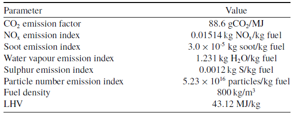
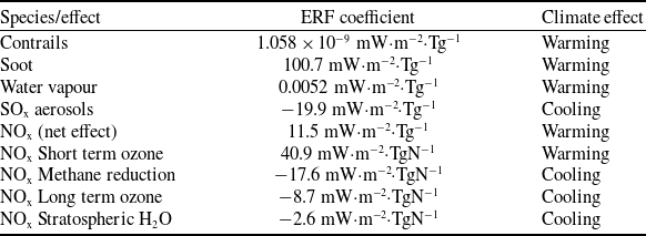

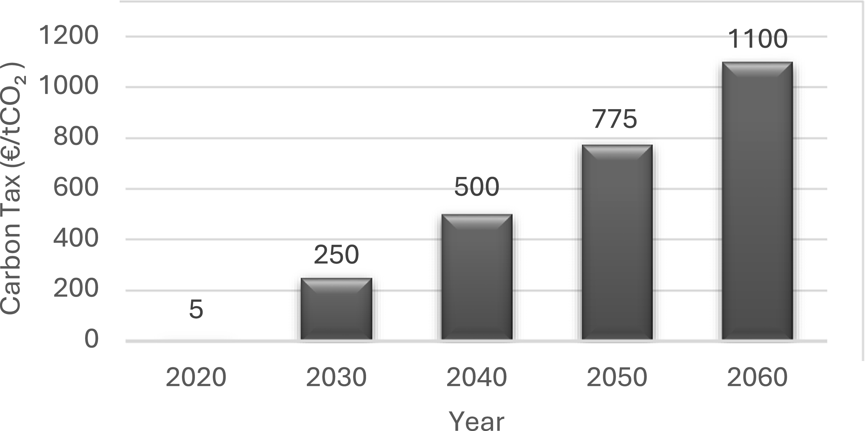
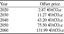
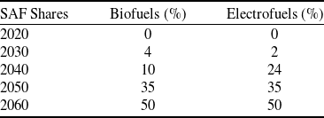
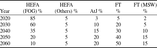
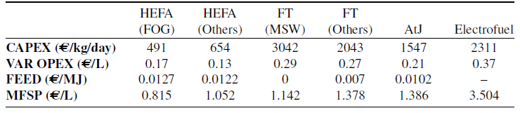
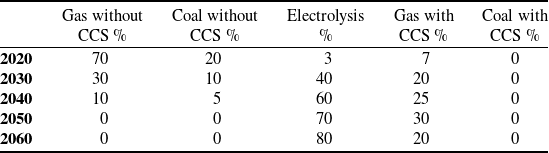
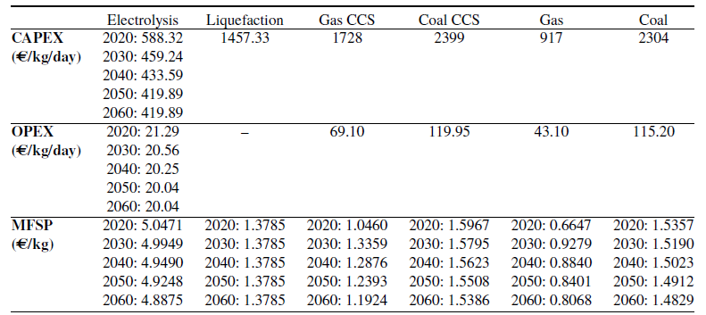


 Open access

