





1. Introduction
Glaciers and ice caps (GICs) along coastal Greenland cover an area of ∼4% of Greenland (Rastner and others, Reference Rastner2012). Despite their relatively small area, the mass loss of the GICs accounted for 14 ± 2% of the total ice loss in Greenland between October 2018 and December 2021 (Khan and others, Reference Khan2022). The contribution is expected to increase in the future because the GICs are considered more sensitive to temperature change than the Greenland ice sheet (Hanna and others, Reference Hanna, Mernild, Cappelen and Steffen2012). The mass loss from Greenland’s GICs has been projected to cause a >10 mm sea-level rise between 2015 and 2100 under the RCP8.5 climate scenario (Marzeion and others, Reference Marzeion2020). Detailed and long-term field observations are required for understanding the mechanisms of glacier change and for more accurate future projections. Nevertheless, glacier monitoring is limited to very few GICs in Greenland (Machguth and others, Reference Machguth2016). Spatially distributed measurements are also essential because satellite remote-sensing data show heterogeneous mass loss of the GICs around Greenland (Hugonnet and others, Reference Hugonnet2021; Khan and others, Reference Khan2022).
Surface mass balance (SMB) measurements have been conducted at Freya Glacier in eastern Greenland since 2007 (Hynek and others, Reference Hynek, Weyss, Binder, Schöner, Jensen, Rasch and Schmidt2013), at Qasigiannguit situated in Kobbefjord in southwestern Greenland since 2012 (Abermann and others, Reference Abermann2019) and at Mittivakkat Glacier in southeastern Greenland since 1995 (Mernild and others, Reference Mernild2013; WGMS, 2025). The annual SMB of Freya Glacier from 2013/14 to 2020/21 was reported as being −0.14 m w.e. a−1, with a decelerating trend in mass loss due to higher winter accumulation between 2014 and 2018 (Hynek and others, Reference Hynek2024). At Qasigiannguit, the annual SMB from 2013 to 2021 was −0.31 m w.e. a−1, with the most negative values recorded in 2016 and 2019 (Messerli and others, Reference Messerli, Arthur, Langley, How and Abermann2022). The longest SMB record was reported from Mittivakkat Glacier, where the ice volume decreased by 29% from 1994 to 2012 (Yde and others, Reference Yde2014). Mernild and others (Reference Mernild2011) attributed the observed mass loss to a decrease in winter precipitation and an increase in summer temperatures.
Since the 1990s, significant warming has been observed in Greenland (Hanna and others, Reference Hanna, Mernild, Cappelen and Steffen2012), which has increased surface melting on the GICs (Box and others, Reference Box, Yang, Bromwich and Bai2009). Glacier changes are also affected by ice dynamics. For example, the decrease in ice flux from upper reaches causes ice thinning in low-elevation areas (e.g. Vincent and others, Reference Vincent, Soruco, Six and Le Meur2009). Near the terminus of Mer de Glace in the French Alps, two-thirds of the acceleration in surface lowering observed between 1979–94 and 2000–08 was attributed to ice dynamics (Berthier and Vincent, Reference Berthier and Vincent2012). In Greenland, the effect of ice dynamics on glacier surface elevation change has rarely been quantified (Mernild and others, Reference Mernild2013).
Because of limited accessibility, glacier research in northwestern Greenland is sparse, even though the need for in situ observation in the region has been highlighted (Machguth and others, Reference Machguth2016). To acquire a long-term record of glacier changes, we have been performing field measurements at Qaanaaq Glacier in northwestern Greenland since 2012 (Sugiyama and others, Reference Sugiyama2014; Tsutaki and others, Reference Tsutaki, Sugiyama, Sakakibara, Aoki and Niwano2017). In this study, we present SMB, ice velocity and surface elevation of Qaanaaq Glacier measured from 2012 to 2025 to quantify the climatic character and the role of SMB and ice dynamics in shaping the observed elevation changes at Qaanaaq Glacier and to understand the mechanism of the mass loss in this region.
2. Study site
Qaanaaq Ice Cap (20–1110 m a.s.l.) is located in northwestern Greenland (77°28′ N, 69°14′ W), covering an area of 258 km2 (Fig. 1). The ice cap has been losing mass from the Little Ice Age (∼1900) to the present time (Carrivick and others, Reference Carrivick, Smith, Sutherland and Grimes2023). Saito and others (Reference Saito, Sugiyama, Tsutaki and Sawagaki2016) reported the mass loss of Qaanaaq Ice Cap from 2007 to 2009 as being −1.5 ± 0.1 m w.e. a−1, indicating an accelerated mass loss from the period 2003–08 (−0.5 ± 0.1 m w.e. a−1 for land-terminating glaciers in northwestern Greenland) (Bolch and others, Reference Bolch2013).
(a) Sentinel-2 MSI images (18–19 August 2023) of the study area in northwestern Greenland. The inset shows the location of the study area in Greenland. The red box indicates the area shown in (b). (b) Satellite image of Qaanaaq Ice Cap. The red box indicates the area shown in (c). (c) The locations of the GNSS reference stations (*), surface mass balance (SMB) and ice velocity measurements (●) and automatic weather station (+). The central flowline and the margin of Qaanaaq Glacier are indicated by solid and dotted lines, respectively. The continuous GNSS measurements used for the uncertainty evaluation were taken at Q1204.

Figure 1 Long description
A) Satellite image of northwestern Greenland with an inset showing the study area. The red box highlights the area shown in B. B) Closer view of Qaanaaq Ice Cap with a red box indicating the area shown in C. C) Detailed map of Qaanaaq Ice Cap with symbols: red dots for SMB and ice velocity measurements, asterisks for GNSS reference stations, plus signs for automatic weather stations and lines for the central flowline and glacier margin. The map includes labeled GNSS stations Q1201, Q1202, Q1203 and Q1204. Scale bars are present in each image for distance reference.
Qaanaaq Glacier is one of the outlet glaciers flowing southward from the interior of the ice cap. This glacier has been the focus of Japanese research projects conducted in the Qaanaaq region since 2011 (Aoki and others, Reference Aoki, Matoba, Uetake, Takeuchi and Motoyama2014; Sugiyama and others, Reference Sugiyama2021, Reference Sugiyama2025). Measurements of SMB, ice velocity and surface elevation have been repeated along the central flowline of the glacier since 2012 (Fig. 1c). Ice thickness and bed elevation were measured along the flowline by radar-echo soundings, which showed the mean and maximum ice thickness to be 120 and 165 m, respectively (Sugiyama and others, Reference Sugiyama2014; Lamsters and others, Reference Lamsters2024). From 2012 to 2016, the mean glacier-wide SMB of Qaanaaq Glacier was −0.22 ± 0.30 m w.e. a−1, which was negatively correlated with summer temperature and positively correlated with annual snowfall (Tsutaki and others, Reference Tsutaki, Sugiyama, Sakakibara, Aoki and Niwano2017). Enhanced surface melt was observed at elevations of 400–500 m a.s.l., suggesting the influence of albedo reduction due to glacial microbes (Sugiyama and others, Reference Sugiyama2014; Takeuchi and others, Reference Takeuchi, Nagatsuka, Uetake and Shimada2014). The annual mean air temperature at Qaanaaq is −8.0℃ at sea level, suggesting that the ice is dominantly cold (Sugiyama and others, Reference Sugiyama2014). However, glacier speedup was observed during some summer seasons, which implied the occurrence of meltwater drainage to the base, probably in the crevassed upper regions (Sugiyama and others, Reference Sugiyama2014; Tsutaki and others, Reference Tsutaki, Sugiyama, Sakakibara, Aoki and Niwano2017). An automatic weather station operates at 944 m a.s.l. (SIGMA-B; 77°31′ N, 69°04′ W) (Fig. 1c) to record meteorological data and snow surface height (Aoki and others, Reference Aoki, Matoba, Uetake, Takeuchi and Motoyama2014; Nishimura and others, Reference Nishimura2023a).
3. Methods
Field measurements were conducted in June–August from 2012 to 2025. SMB and ice flow velocity were measured at six survey sites situated approximately along the central flowline at 243–984 m a.s.l., as measured in August 2025 (Q1201–Q1206 in Fig. 1c). The measurements were performed by surveying aluminum poles installed in the ice using an electric drill (Makita HR262DRDX) and an auger (Kovacs). Surface elevation measurements were carried out along the central flowline of the glacier (Fig. 1c).
3.1. Surface mass balance
The annual mass balance was obtained by reading the height of the poles above the glacier surface in late July or early August (Table S1). Ice and water densities of 917 and 1000 kg m−3, respectively, were used to convert ice thickness to water equivalent. In the area covered by snow, snow depth and density were measured by weighing snow samples collected with a 100 cm3 snow cutter. Considering the uncertainty in the snow density (±50 kg m−3) and stake reading error (±0.02 m w.e.; Cogley and others, Reference Cogley, Adams, Ecclestone, Jung-Rothenhäusler and Ommanney1996; Tsutaki and others, Reference Tsutaki, Sugiyama, Sakakibara, Aoki and Niwano2017), the uncertainty in our annual SMB data was 0.02–0.12 m w.e.
In 2020, stake measurements were performed on 26 June due to the influence of COVID-19. Thus, we estimated SMB from 26 June to 1 August in 2020 at each site with a surface energy-balance melt model (Kondo and others, Reference Kondo, Sugiyama, Sakakibara and Fukumoto2021), using data from the weather station at SIGMA-B (Fig. 1c). In turn, the mass balance in 2019/20 and 2020/21 was determined from these values to align the mass-balance year. The root mean square error of the melt model (0.10 m w.e.) was considered an additional uncertainty for the mass balance in 2019/20 and 2020/21.
Based on the observed annual SMB, we estimated the glacier-wide/ice-cap-wide SMB of Qaanaaq Glacier (B QG) and Ice Cap (B QIC) as
 \begin{equation}{B_{{\text{QG}}/{\text{QIC}}}} = \,\frac{{{ \sum_Z}{S_Z}{b_Z}}}{S},\end{equation}
where S is the catchment area, Sz and bz are the surface area and SMB for each 50 m elevation band z. S and Sz were calculated using glacier margins delineated on the Landsat 8 satellite image acquired in August 2023 and surface elevation data from ArcticDEM Mosaic Version 4.1, with a horizontal resolution of 32 m (Porter and others, Reference Porter2023). The digital elevation model (DEM) was composed based on data acquired between 2007 and 2022, and therefore represents the topography during our study period 2012–25. The margin of Qaanaaq Glacier was determined by processing a DEM with GIS software (QGIS) (Fig. 1c, the dotted line). In this study, B QG and B QIC were calculated using fixed glacier margins because changes in glacier margins over the study period are small. SMB at each elevation band (bz) was calculated by linearly interpolating the observations at Q1201–Q1206. SMB above Q1206 and below Q1201 was estimated by (1) assuming the values observed at Q1201 and Q1206 and (2) linearly extrapolating the observations. The difference between (1) and (2) was understood as the uncertainty of the estimation.
3.2. Ice velocities
Annual and summer ice velocities at Q1201–Q1206 were measured by surveying the mass balance poles twice in summer, once at the beginning and once at the end of the field campaigns (Tables S2 and S3). An antenna of Global Navigation Satellite System (GNSS) (Leica GS10, System1200; or Enabler Ltd, GEM-1) was mounted on the top of the pole to record dual-frequency GNSS signals for ∼30 min with a sampling frequency of 1 s. Using GNSS data recorded at a reference station established in Qaanaaq Village (Fig. 1c), three-dimensional coordinates of the stakes were computed in a static mode with GNSS software RTKLIB (https://www.rtklib.com/rtklib.htm, last access 13 November 2025) or Leica Infinity (Leica Geosystems). The baseline length was 2.5–7.5 km, and the maximum elevation change from the reference station was 945 m. Annual and summer velocities in horizontal and vertical directions were obtained from the stake displacement. Velocities are unavailable for the 2020–2022 period because no survey was conducted in 2021. By analyzing GNSS data continuously recorded at Q1204 (Fig. 1c), uncertainties in GNSS positioning were estimated as 8 and 21 mm in the horizontal and vertical directions, respectively. The poles froze in cold ice after installation; thus, we assume no influence of their tilting on the survey.
To investigate the contribution of ice dynamics to surface elevation change, the emergence velocity ( ${v_{\text{e}}}$) was calculated as (Cuffey and Paterson, Reference Cuffey and Paterson2010)
 \begin{equation}\begin{array}{*{20}{c}}
{{v_{\text{e}}} = {\text{ }}{w_{\text{s}}} - {u_{\text{s}}}\frac{{\partial h}}{{\partial x}},{\text{ }}}
\end{array}\end{equation}
where  ${w_{\text{s}}}$ and
 ${u_{\text{s}}}$ are the measured vertical and horizontal surface velocities, respectively, and
 $\partial h/\partial x$ is a surface slope along the flow direction based on ArcticDEM Mosaic Version 4.1 (2 m resolution) (Porter and others, Reference Porter2023).
3.3. Surface elevation
On 26–30 July 2012, 3 August 2019, and 15–16 August 2025, we measured glacier surface elevation at 280 locations along the glacier flowline spanning the survey sites from the glacier front to Q1206 (Fig. 1c). The GNSS instruments and software described in subsection 3.2 were used for this measurement. GNSS signals were recorded at each survey site for ∼30 s with a sampling interval of 1 s and processed in a kinematic mode with data from the reference station (Fig. 1c). Based on the kinematic processing of the continuous data from Q1204, the uncertainties in the horizontal and vertical coordinates were 7 and 13 mm, respectively. The same locations were resurveyed in 2019 and 2025, by locating the 2012 survey sites using a handheld GNSS device (Garmin eTrex) with a horizontal accuracy of 5–10 m.
The rate of surface elevation change was calculated for 2012–19 and 2019–25, and its dependence on altitude was analyzed by filtering the survey data with a local linear regression routine using a 100 m bandwidth. To minimize the effect of resurveyed locations, we excluded data from the calculations if the horizontal offset exceeded 2 m.
3.4. Meteorological data
Air temperature and relative glacier surface height were recorded every hour using a temperature sensor (Vaisala, HMP115) and an ultrasonic ranger (Campbell, SR50) at a height of 3 m above the surface at SIGMA-B (Fig. 1c) (Nishimura and others, Reference Nishimura2023a). Air temperature during 2012–20 was obtained from Nishimura and others (Reference Nishimura2023c), relative glacier surface height during 2012–20 from Nishimura and others (Reference Nishimura2023b) and the data during 2020–25 from Arctic Data Archive System (ADS) (https://ads.nipr.ac.jp/real-time-monitors/sigma-b/, last access 13 November 2025). The daily mean temperature and the summer (June/July/August) mean temperature (SMT) were computed from the hourly data. Changes in the glacier surface height were used to estimate snow accumulation in each mass balance year, by assuming a fresh snow density of 120 ± 50 kg m−3 (Jones and others, Reference Jones, Pomeroy, Walker and Hoham2001).
The summer (June/July/August) and winter (December/January/February) North Atlantic Oscillation (NAO) indices (https://www.ncei.noaa.gov/access/monitoring/nao/, last access 7 April 2026) were compared with SMB to discuss the relationship between a glacier-wide SMB and atmospheric circulation.
4. Results
4.1. Surface mass balance
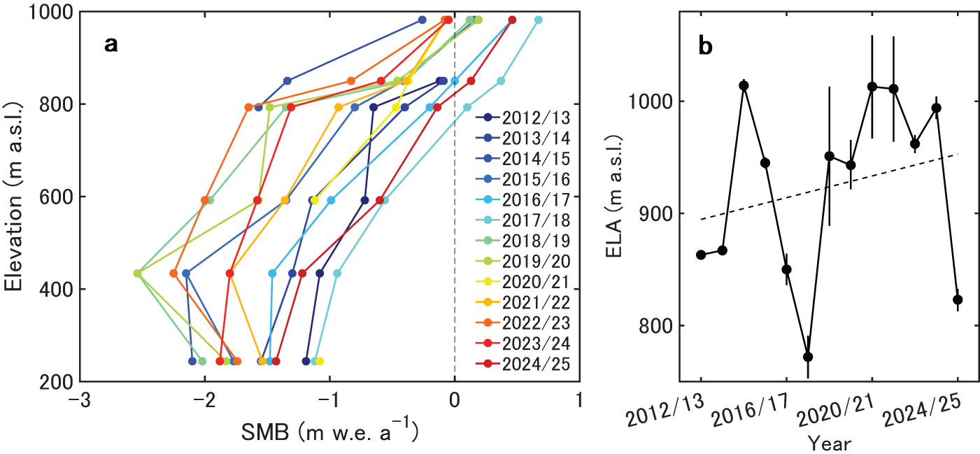
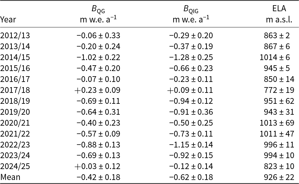
The SMB averaged over the 13 years was −1.59 ± 0.05 m w.e. a−1 at Q1201 and 0.14 ± 0.11 m w.e. a−1 at Q1206 (Table 1). The most negative mass balance was observed at the second lowest site, Q1202 (−1.77 ± 0.05 m w.e. a−1). SMB at Q1202 was more negative than at Q1201, particularly between 2018 and 2023 (Table 1 and Fig. 2a). This result consists with previous studies, which pointed out the influence of albedo reduction due to glacial microbes at Q1202 (Sugiyama and others, Reference Sugiyama2014; Takeuchi and others, Reference Takeuchi, Nagatsuka, Uetake and Shimada2014). In addition to the albedo effect, mass balance in the lower reaches of the glacier may be influenced by temperature inversion frequently observed along the Greenlandic coast (Shahi and others, Reference Shahi, Abermann, Heinrich, Prinz and Schöner2020). The mean equilibrium line altitude (ELA) from 2012 to 2025 was 926 ± 22 m a.s.l., and ELAs since 2018/19 were higher than the mean over the study period, except for 2024/25 (Fig. 2b and Table 2). The regression of the data shows an ascending trend in the ELA (48 m decade−1), although the year-to-year variations are substantially large (from 772 to 1014 m a.s.l.).
SMB at Q1201–Q1206.

Table 1 Long description
Annual surface mass balance values (meters water equivalent per year) are listed for six sites from 243 to 984 meters elevation for years 2012/13 through 2024/25, with uncertainties. A clear elevation gradient appears: lower sites are consistently more negative, while the highest site is near zero or positive in several years. Mean values by site are minus 1.59 at 243 meters, minus 1.77 at 434 meters, minus 1.25 at 592 meters, minus 0.83 at 747 meters, minus 0.35 at 850 meters, and plus 0.14 at 984 meters. The most negative single-year values occur at mid to low elevations, including minus 2.54 at 434 meters in 2018/19 and again in 2019/20, and minus 2.10 at 243 meters in 2014/15. The highest site shows positive years such as 2016/17 (plus 0.46), 2017/18 (plus 0.67), and 2024/25 (plus 0.46), but is slightly negative in some recent years (for example minus 0.08 in 2022/23). Several years have missing entries (for example Q1206 in 2012/13 and 2013/14, Q1203 in 2014/15, and Q1202 in 2020/21), so comparisons across all sites are not always possible. Overall, the table indicates persistent net loss at lower elevations and more balanced conditions at higher elevations, with strong year-to-year variability.
(a) Annual SMB at Q1201–Q1206 from 2012 to 2025. (b) Estimated ELA from 2012 to 2025. The dashed line represents the linear regression of the data.

Figure 2 Long description
The image A showing a line graph. The horizontal axis label is “SMB (m w.e. a superscript minus 1)” with tick labels negative 3, negative 2, negative 1, 0, 1. The vertical axis label is “Elevation (m a.s.l.)” with tick labels 200, 400, 600, 800, 1000. A legend lists 2012 slash 13, 2013 slash 14, 2014 slash 15, 2015 slash 16, 2016 slash 17, 2017 slash 18, 2018 slash 19, 2019 slash 20, 2020 slash 21, 2021 slash 22, 2022 slash 23, 2023 slash 24, 2024 slash 25. Each year is shown as a separate connected line with circular markers. The plotted SMB values extend from negative 3 to 1 and the plotted elevations extend from 200 to 1000. Across the year series, SMB values are more negative at lower elevations and move toward 0 and positive values at higher elevations, with several series reaching near 0 to 1 at elevations near 900 to 1000. The image B showing a line graph. The horizontal axis label is “Year” with tick labels 2012 slash 13, 2016 slash 17, 2020 slash 21, 2024 slash 25. The vertical axis label is “ELA (m a.s.l.)” with tick labels 800, 900, 1000. A connected line with circular markers shows ELA values varying between the 800 and 1000 tick marks across the years. Several points include vertical error bars. A dashed line runs upward across the plot. Both graphs use yearly series to show changes over time. The first graph shows SMB profiles by elevation for each year and the second graph shows ELA by year with a dashed line.
The glacier-wide/ice-cap-wide surface mass balance of Qaanaaq Glacier (B QG)/Ice Cap (B QIG), and ELA for the balance years 2012–25.

Table 2 Long description
Annual surface mass balance for Qaanaaq Glacier and the wider Ice Cap is listed for balance years 2012/13 through 2024/25, along with the equilibrium line altitude, all reported with uncertainty ranges. Mean mass balance is negative for both, with the Ice Cap more negative than the glacier on average. The largest losses occur in 2014/15, when both glacier and ice cap reach their most negative values and the equilibrium line altitude is among the highest. The only year with clearly positive mass balance for both is 2017/18, which also has the lowest equilibrium line altitude in the series. In 2024/25 the glacier is near zero to slightly positive while the ice cap remains slightly negative, and the equilibrium line altitude is relatively low compared with most other years. Across most years, higher equilibrium line altitude generally coincides with more negative mass balance, but the uncertainties indicate year to year differences should be interpreted cautiously.
The glacier-wide SMB (B QG) showed a mass loss of −5.43 ± 0.38 m w.e. from 2012 to 2025. Annual mass balance was characterized by significant year-to-year variations from −1.02 ± 0.22 m w.e. a−1 in 2014/15 to 0.23 ± 0.09 m w.e. a−1 in 2017/18 (Fig. 3 and Table 2). The mean annual balance was −0.42 ± 0.18 m w.e. a−1 with a standard deviation (SD) of 0.38 m w.e. a−1.
The glacier-wide annual (cyan, left axis) and cumulative (red, right axis) SMB of Qaanaaq Glacier for the balance years 2012/13–2024/25.

Figure 3 Long description
A mixed bar and line graph. Horizontal axis label: Balance year. Tick labels shown: 2012 slash 13, 2016 slash 17, 2020 slash 21, 2024 slash 25. Left vertical axis label: Glacier-wide SMB (m w.e. a superscript minus 1). Tick labels shown: 0.4, 0.2, 0, minus 0.2, minus 0.4, minus 0.6, minus 0.8, minus 1. Right vertical axis label: Cumulative mass balance (m w.e.). Tick labels shown: 0, minus 1, minus 2, minus 3, minus 4, minus 5, minus 6. Bars: One bar per balance year from 2012 slash 13 through 2024 slash 25. Most bars extend below the zero line on the left axis. One bar near the middle extends above zero to slightly above 0.2. The final bar at 2024 slash 25 extends slightly above zero. Line with circular markers: One marker per balance year from 2012 slash 13 through 2024 slash 25, plotted against the right axis. The first marker is near 0. The line descends across the years, reaching near minus 5 by 2023 slash 24 and the final marker at 2024 slash 25 is at a similar level near minus 5. A dashed horizontal line is drawn near the 0 level on the right axis.
The ice-cap-wide SMB (B QIC) exhibited similar year-to-year variations (from −1.28 ± 0.25 to 0.09 ± 0.11 m w.e. a−1) as observed for Qaanaaq Glacier (Table 2). From 2012 to 2025, the cumulative mass balance of Qaanaaq Ice Cap was −8.01 ± 0.22 m w.e. (−0.62 ± 0.18 m w.e. a−1). The mean B QIC from 2012 to 2020 (−0.57 ± 0.20 m w.e. a−1) agrees with the geodetic mass balance reported for Qaanaaq Ice Cap between 2010 and 2020 (−0.50 ± 0.17 m w.e. a−1) (Hugonnet and others, Reference Hugonnet2021) within the uncertainty range. The mean mass loss from 2020 to 2025 (−0.68 ± 0.16 m w.e. a−1) was 19% greater than that of the period 2012–20. The elevation-dependent scaling neglects several processes including the influence of the slope aspect on radiation and the spatiotemporal variabilities in surface albedo as pointed out in the study area (Traversa and others, Reference Traversa2025). Therefore, although we are confident about the long-term mass loss of the ice cap, care should be taken when interpreting year-to-year variations and spatial variabilities.
4.2. Ice velocities
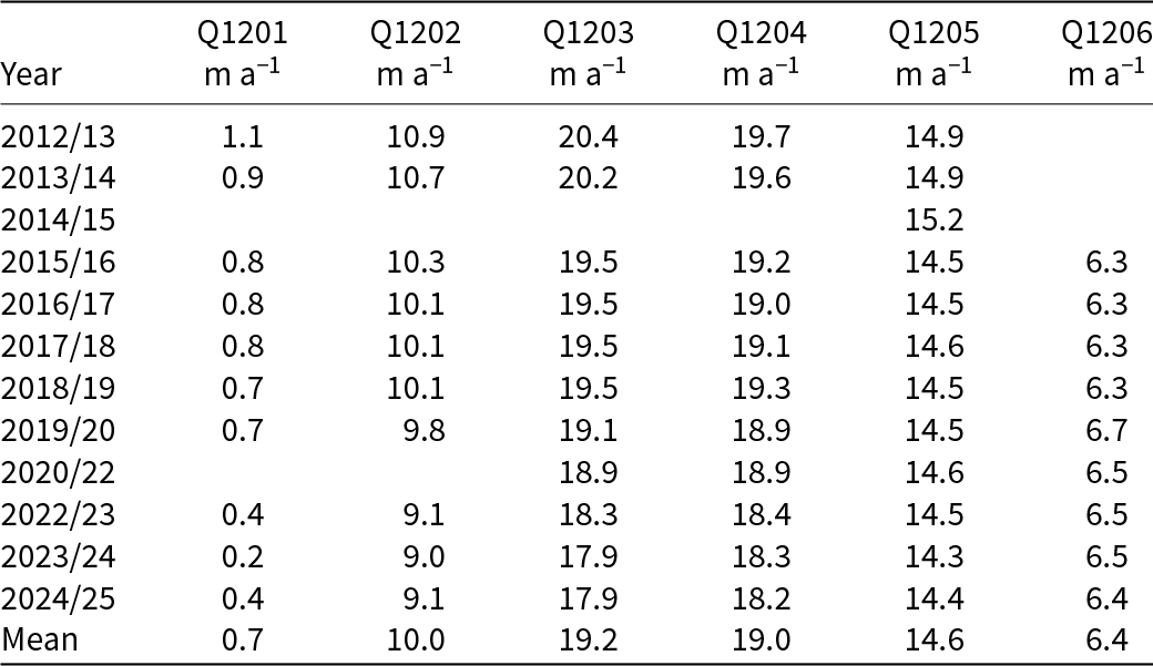
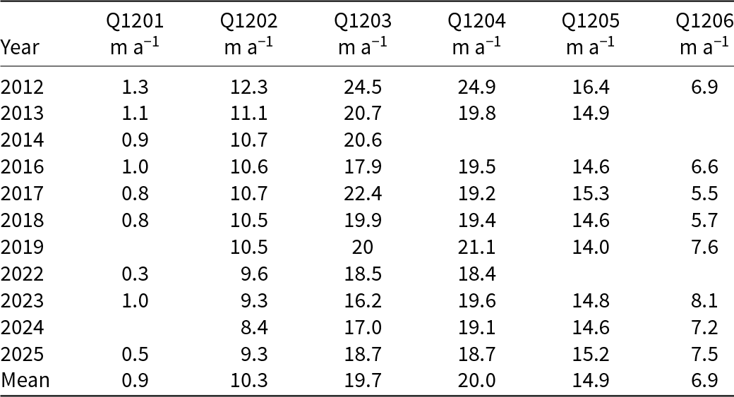
The fastest ice flow was observed at Q1203 and Q1204 (Fig. 4c). Annual velocities at Q1201–Q1204 decreased by 64%, 17%, 12% and 8% from 2012 to 2025, whereas those at the upper two sites (Q1205 and Q1206) varied within 2–3%, showing an insignificant trend over the study period (Figs 4a–e and Table 3). Summer ice velocities showed decreasing trends, except for the upper sites (Q1205 and Q1206), where the change was insignificant (Table 4). Summer velocities in 2012 were notably higher than those in other years. For example, velocities at Q1203 and Q1204 in the summer of 2012 exceeded the 13-year mean by 24% and 25%, respectively.
(a–e) Annual horizontal velocity and (f) emergence velocity at Q1201–Q1206 in 2012/13–2024/25. The dashed lines in (f) indicate linear regressions.

Figure 4 Long description
The multi-line graph consists of six panels labeled a to f. Panels a to e display annual horizontal velocity (m a superscript minus 1) for sites Q1201 to Q1206. The horizontal axis represents the year, ranging from 2012 to 2024. Panel a shows Q1201 with a gradual decline from 1.5 to 0.5. Panel b shows Q1202 decreasing from 10.5 to 9. Panel c includes Q1203 and Q1204, both starting around 20.5 and trending downward to approximately 18. Panel d shows Q1205 with a slight decrease from 15.5 to 14. Panel e shows Q1206 remaining stable around 6.5. Panel f displays emergence velocity (m a superscript minus 1) for all sites. Q1201 and Q1202 show a slight decline, while Q1203 and Q1204 fluctuate with a downward trend. Q1205 and Q1206 show negative values increasing toward zero. The lines are distinguished by solid and dashed styles, with error bars indicating variability. The dashed lines in panel f represent linear regressions, highlighting trends over time. The graph illustrates the overall decline in velocities, with Q1203 and Q1204 showing the most significant changes.
Annual horizontal velocities at Q1201–Q1206.

Table 3 Long description
The table lists annual horizontal velocities, in meters per year, for six locations labeled Q1201 through Q1206 across years from 2012/13 to 2024/25, plus a mean row. Q1203 and Q1204 are consistently the fastest sites, starting near 20 meters per year in 2012/13 and decreasing to about 18 meters per year by 2023/24 and 2024/25. Q1202 shows a gradual decline from about 10.9 meters per year in 2012/13 to about 9.0 to 9.1 meters per year in 2023/24 and 2024/25. Q1201 is the slowest and trends downward overall, from 1.1 meters per year in 2012/13 to 0.2 in 2023/24, with a small rebound to 0.4 in 2024/25. Q1205 remains relatively stable around the mid 14 meters per year range, varying from about 14.3 to 15.2 across the period. Q1206 is only reported from 2015/16 onward and stays near 6.3 to 6.7 meters per year, ending at 6.4 in 2024/25. Several entries are missing, including all sites except Q1205 in 2014/15 and some sites in 2020/22, so trends should be interpreted with those gaps in mind.
Summer horizontal velocities at Q1201–Q1206.

Table 4 Long description
The table lists summer horizontal velocities, in meters per year, for six locations labeled Q1201 through Q1206 across multiple years, plus a mean row. Average velocities rise from Q1201 at 0.9 to Q1202 at 10.3, peak at Q1203 at 19.7 and Q1204 at 20.0, then drop to Q1205 at 14.9 and Q1206 at 6.9. The largest single value is 24.9 at Q1204 in 2012, with Q1203 also high in 2012 at 24.5. Q1202 generally declines over time from 12.3 in 2012 to 8.4 in 2024, while Q1203 and Q1204 fluctuate around the high teens to low twenties, including a low of 16.2 at Q1203 in 2023 and a high of 22.4 at Q1203 in 2017. Q1206 varies from 5.5 in 2017 to 8.1 in 2023, and Q1201 stays near 1 or below when reported, reaching 0.3 in 2022. Several cells are blank for some years and sites, so year to year comparisons may reflect missing observations rather than true change.
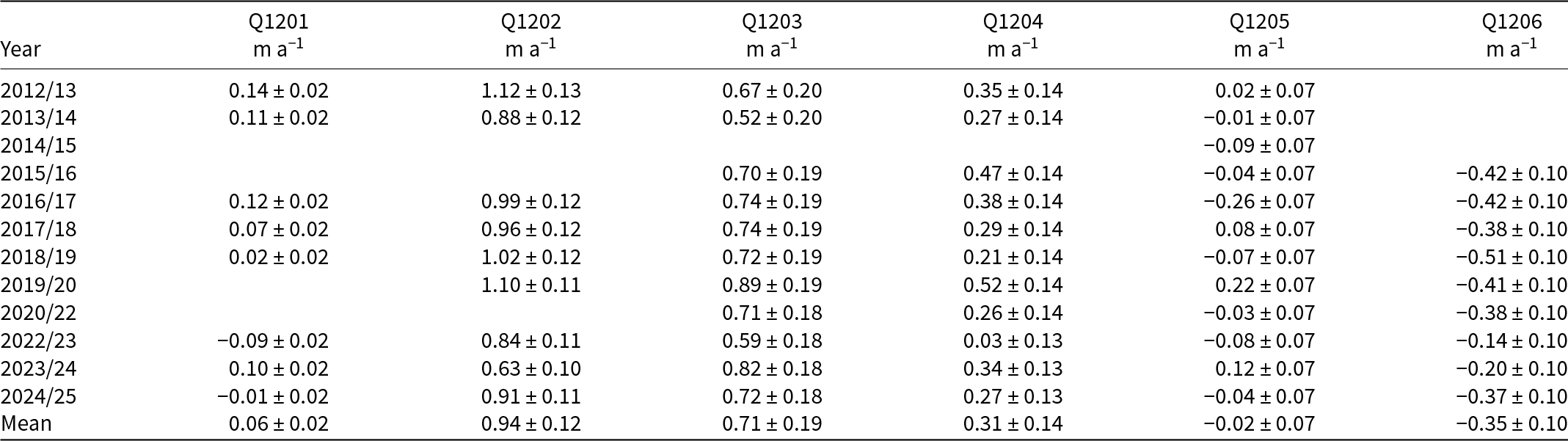
The emergence velocities averaged from 2012 to 2025 ranged from −0.35 ± 0.10 m a−1 at Q1206 to 0.94 ± 0.12 m a−1 at Q1202 (Fig. 4f and Table 5). The velocities were negative (downward) in the upper regions at Q1205 and Q1206, whereas they were positive (upward) at the other sites in the lower reaches. The upward velocity at Q1202 decreased from 1.12 ± 0.13 m a−1 in 2012/13 to 0.91 ± 0.11 m a−1 in 2024/25 with a trend of −0.02 ± 0.03 m a−2. The downward velocity at Q1206 also showed a decreasing trend of 0.02 ± 0.03 m a−2.
Emergence velocities at Q1201–Q1206.

Table 5 Long description
The table reports annual emergence velocities, in meters per year with plus or minus uncertainty, for six locations labeled Q1201 through Q1206 across multiple years from 2012 to 2024, plus a mean row. Q1202 is the largest and most consistently positive series, ranging from about 0.63 to 1.12, with a mean near 0.94. Q1203 is also consistently positive where reported, typically around 0.52 to 0.89, with a mean near 0.71. Q1204 stays positive but smaller, roughly 0.03 to 0.52, averaging about 0.31. Q1201 is small and near zero overall, including negative years such as 2022 to 2023 and 2024 to 2025, with a mean near 0.06. Q1205 fluctuates around zero, with both small positives and negatives, and a mean near minus 0.02. Q1206 is negative in every year it is reported, roughly minus 0.14 to minus 0.51, averaging about minus 0.35. Several cells are blank, so comparisons across years should be interpreted as limited to the years with measurements.
4.3. Surface elevation change
Surface elevation has decreased across the entire study region (Fig. 5a). The elevation changes from 2012 to 2025 ranged from −20.5 m at 258 m a.s.l. to −0.7 m at 988 m a.s.l., with a mean of −8.7 m (−0.67 m a−1) along the survey route. The SD of the observed data from the smoothing curve was 0.58 m (0.04 m a−1). The change was more pronounced downglacier, particularly in the lower reaches (<500 m a.s.l.) (Fig. 5a).
(a) Surface elevation change from 2012 to 2025, and (b) the elevation change rate from 2012 to 2019 (blue) and from 2019 to 2025 (red) along the central flowline of Qaanaaq Glacier (Fig. 1c). Local regressions of the data are given by the solid curves.

Figure 5 Long description
The image A showing a scatter plot with a fitted curve and a legend. The horizontal axis label is Elevation (m a.s.l.). The horizontal axis shows 200, 400, 600, 800, 1000. The vertical axis label is Elevation change (m). The vertical axis shows 0, minus 4, minus 8, minus 12, minus 16, minus 20. A dashed horizontal line is drawn at 0. The legend lists Observed and Smoothed. A bold letter a appears near the upper left of the plot area. Observed points and the smoothed curve extend from about (250, minus 20) upward to about (950, near 0). Points are clustered around elevations roughly 450 to 900 with elevation change values roughly minus 9 to minus 2. The image B showing a scatter plot with two fitted curves and a legend. The horizontal axis label is Elevation (m a.s.l.). The horizontal axis shows 200, 400, 600, 800, 1000. The vertical axis label is Elevation change rate (m a superscript minus 1). The vertical axis shows 0, minus 0.4, minus 0.8, minus 1.2, minus 1.6, minus 2. A dashed horizontal line is drawn at 0. The legend lists 2012 dash 2019 and 2019 dash 2025. A bold letter b appears near the upper left of the plot area. Both series of points and their fitted curves extend from about (250, about minus 1.8 to minus 2.0) upward to about (950, about minus 0.2 to minus 0.3). Around elevation 400, values are around minus 1.2 to minus 1.0. Around elevation 600, values are around minus 0.7 to minus 0.5. Around elevation 800, values are around minus 0.5 to minus 0.3.
In terms of the mean values across the study area, downward surface elevation change accelerated by 18% from −0.69 m a−1 in 2012–19 to −0.81 m a−1 in 2019–25 (Fig. 5b). The acceleration in the lower (<500 m a.s.l.) and middle (500–800 m a.s.l.) elevation areas was 12% (from −1.14 to −1.30 m a−1) and 20% (from −0.50 to −0.62 m a−1), respectively. In contrast to those regions, the change between the two periods was insignificant in the upper reaches (>800 m a.s.l.) (Fig. 5b).
4.4. Meteorological data
Over the study period, mean SMT and annual snowfall at SIGMA-B were 0.5℃ and 0.41 ± 0.16 m w.e. a−1, respectively (Fig. 6a). The glacier-wide SMB in each year was inversely correlated with SMT (correlation coefficient: r = −0.83, statistical significance: p < 0.01) (Fig. S1a). The correlation with annual snowfall was insignificant from 2012/13 to 2024/25 (r = 0.25, p = 0.41) (Fig. S1b), whereas it was positive from 2012/13 to 2018/19 (r = 0.81, p = 0.03).
(a) Summer mean temperature (red) and annual snowfall (blue) at SIGMA-B, (b) glacier-wide SMB of Qaanaaq Glacier and (c) summer (orange) and winter (cyan) NAO indices during the period 2012–25.

Figure 6 Long description
The image consists of three panels, each displaying a multi-line graph over the balance years 2012 to 2025. Panel a: The x-axis represents the balance year and the y-axes show summer mean temperature in degrees Celsius on the left and snowfall in meters water equivalent per year on the right. The red line represents summer mean temperature and the blue line represents snowfall. Notable points include a peak in temperature around 2016/17 and a dip in snowfall around 2018/19. Error bars are present for snowfall data. Panel b: The x-axis is the balance year and the y-axis represents glacier-wide SMB in meters water equivalent per year. The black line shows variations in SMB, with a notable low around 2014/15 and a rise towards 2024/25. Error bars are included. Panel c: The x-axis is the balance year and the y-axis shows the NAO index. The orange line represents the summer NAO index and the cyan line represents the winter NAO index. Key observations include fluctuations in both indices, with a peak in the summer index around 2018/19 and a dip in the winter index around 2014/15. The graphs illustrate trends and variations in climate-related data over the specified period.
Mean summer and winter NAO indices over the study period were −0.18 and 0.82, respectively (Fig. 6c). The glacier-wide SMB was positively correlated with the summer NAO index (r = 0.69, p < 0.01), whereas the correlation with the winter NAO index was insignificant (r = −0.25, p = 0.41).
5. Discussion
5.1. Sensitivities of SMB to air temperature and snowfall
The glacier-wide SMB of Qaanaaq Glacier showed a stronger correlation with SMT than with snowfall over the study period (Figs S1a and S1b). To better understand the sensitivities of SMB to air temperature and snowfall, we conducted a multiple linear regression analysis, assuming linear dependence of SMB B QG (m w.e. a−1) on SMT T (℃) and snowfall A (m w.e. a−1).
 \begin{equation}\begin{array}{*{20}{c}}
{{B_{{\text{QG}}}} = - 0.35T + 1.18A - 0.70}
\end{array}\end{equation}
The F-value (significance of the regression model) of Eq. (3) was 13.3 (p < 0.01), indicating that the dependence on SMT T (℃) and snowfall A (m w.e. a−1) is statistically significant. This model reproduced the observations from 2012/13 to 2024/25 with a root mean square error of 0.19 m w.e. a−1, a coefficient of determination of 0.73 and a p-value of <0.01 (Fig. 7). Considering the t-values (relative contributions to the glacier-wide SMB) of T (−4.9) and A (1.1), statistically speaking, the glacier-wide SMB of Qaanaaq Glacier is about five times more influenced by SMT (i.e. ablation) than by snowfall (i.e. accumulation).
Scatter plot of observed and modeled glacier-wide SMB of Qaanaaq Glacier in 2012/13–2024/25. The coefficient of determination (r 2) and the p-value between modeled and observed glacier-wide SMB are given.

The sensitivities of the glacier-wide SMB of Qaanaaq Glacier were −0.35 m w.e. a−1 for 1℃ warming and +0.05 m w.e. a−1 for a 10% snowfall increase. In the nearby Prudhoe Land region, the sensitivity of marine-terminating glacier ice loss to air temperature was reported as −0.56 m w.e. a−1 ℃−1 (Wang and others, Reference Wang, Sugiyama and Bjørk2021). Mass loss of marine-terminating glaciers is 1.6 times more sensitive to the changing climate of northwestern Greenland, driven not only by SMB but also by other factors, including calving and frontal ablation (Moon and others, Reference Moon, Joughin, Smith and Howat2012).
Qaanaaq Glacier’s mass balance sensitivity to air temperature (−0.38 m a−1 ℃−1) was similar to the mean value of −0.37 m a−1 ℃−1 (Dyurgerov and Meier, Reference Dyurgerov and Meier2000) of those reported for glaciers worldwide, which range from −0.1 to −1.3 m a−1 ℃−1 (Oerlemans and Fortuin, Reference Oerlemans and Fortuin1992; Braithwaite and Zhang, Reference Braithwaite and Zhang1999). A 10% increase in snowfall offsets 14% of the mass loss due to a warming of +1℃, which is, however, lower than ∼20% offset reported for other Arctic GICs (de Woul and Hock, Reference de Woul and Hock2005). Given the amplification of warming in the Arctic (e.g. Rantanen and others, Reference Rantanen2022), the mass loss of glaciers in the study region will be increasingly important in the future.
5.2. Comparison with SMB of other glaciers in coastal Greenland
The SMB obtained for Qaanaaq Glacier from 2012 to 2025 was compared with those of three other Greenlandic glaciers reported to the World Glacier Monitoring Service (WGMS, 2025; Fig. 8). From 2012 to 2023, the period overlapping SMB measurements at four glaciers, the annual mean SMBs were −0.43 m w.e. a−1 at Qaanaaq Glacier, −0.38 m w.e. a−1 at Freya Glacier, −1.15 m w.e. a−1 at Mittivakkat Glacier and −0.64 m w.e. a−1 at Qasigiannguit Glacier, respectively. Mittivakkat Glacier showed the largest mass loss, i.e. 76% greater than the mean of the four other glaciers (−0.65 m w.e. a−1).
The glacier-wide SMBs of coastal Greenland from 2012 to 2025. The colored dots on the map show the locations of the glaciers.

The SMB of the glaciers showed large year-to-year variations (Fig. 8). The SDs of the annual SMB were 0.38, 0.69, 0.59 and 0.75 m w.e. a−1 for Qaanaaq, Freya, Mittivakkat and Qasigiannguit Glaciers, respectively. Further, year-to-year variations did not correlate with each other. The correlation with the value of Qaanaaq Glacier was r = 0.39 (p = 0.22) for Freya Glacier, r = 0.13 (p = 0.70) for Mittivakkat Glacier and r = 0.32 (p = 0.34) for Qasigiannguit Glacier.
Comparisons of NAO indices with glacier-wide SMBs provided insight into the mechanisms driving the regionally different SMB (Fig. 9). In western Greenland (Qaanaaq and Qasigiannguit Glaciers), SMB showed a significant correlation with the summer NAO index (r = 0.69; p < 0.01 and r = 0.53; p = 0.10) as reported by Bevis and others (Reference Bevis2019), whereas the correlations for glaciers in eastern Greenland (Freya and Mittivakkat Glaciers) were insignificant (r = 0.19; p = 0.54 and r = 0.19; p = 0.56). In contrast, the winter NAO index correlated with SMB in eastern Greenland, but not in western Greenland (Fig. 9). The summer NAO index is associated with enhanced melting due to clear-sky and drier conditions (Box and others, Reference Box2012; Fettweis and others, Reference Fettweis2013). The winter NAO index is positively and negatively correlated with annual accumulation in eastern and western Greenland, respectively (Bjørk and others, Reference Bjørk2018). Therefore, the significant correlation between the summer NAO index and SMB of Qaanaaq Glacier, which is significantly associated with SMT, suggests that SMB in western Greenland is more influenced by ablation than accumulation. On the other hand, we assume that accumulation plays a more important role than melting for SMB in eastern Greenland (Hugonnet and others, Reference Hugonnet2021; Khan and others, Reference Khan2022). Therefore, the results indicate that spatially nonuniform glacier mass loss in Greenland is affected by regionally different atmospheric circulations and their influence on SMB. For a more accurate understanding of the processes, long-term observations distributed over Greenland are essential.
Scatter plots of annual mass balance of (a–b) Qaanaaq, (c–d) Qasigiannguit, (e–f) Freya and (g–h) Mittivakkat Glaciers vs summer and winter NAO indices. Linear regressions of the data are given by the dashed lines with the correlation coefficients (r) and p-values.

Figure 9 Long description
The image A showing a scatter plot of Qaanaaq (m w.e.) versus Summer NAO index, with a dashed regression line. Text: r equals 0.69; (p less than 0.01). Horizontal axis label: Summer NAO index, range negative 1.5 to 1.5. Vertical axis label: Qaanaaq (m w.e.), tick labels 0, minus 0.5, minus 1. Plotted points appear at approximately: (negative 1.5, minus 1.0), (negative 1.5, minus 0.9), (negative 1.5, minus 0.7), (negative 1.5, minus 0.5), (negative 1.2, minus 0.2), (negative 0.6, minus 0.6), (negative 0.1, minus 0.1), (0.2, minus 0.4), (0.3, 0.0), (0.4, minus 0.6), (0.6, minus 0.2), (0.7, minus 0.7), (1.4, 0.2). The dashed line slopes upward. The image B showing a scatter plot of Qaanaaq (m w.e.) versus Winter NAO index, with a dashed regression line. Text: r equals minus 0.25; (p equals 0.41). Horizontal axis label: Winter NAO index, range negative 0.5 to 1.5. Vertical axis label: Qaanaaq (m w.e.), tick labels 0, minus 0.5, minus 1. Plotted points appear at approximately: (negative 0.4, minus 0.4), (0.1, minus 0.1), (0.6, minus 0.1), (0.7, 0.0), (0.8, minus 0.2), (0.8, minus 0.8), (1.0, minus 0.6), (1.1, minus 0.5), (1.2, 0.2), (1.2, minus 0.6), (1.5, minus 1.0). The dashed line slopes downward. The image C showing a scatter plot of Qasigiannguit (m w.e.) versus Summer NAO index, with a dashed regression line. Text: r equals 0.53; (p equals 0.10). Horizontal axis label: Summer NAO index, range negative 1.5 to 1.5. Vertical axis label: Qasigiannguit (m w.e.), tick labels 0, minus 1, minus 2. Plotted points appear at approximately: (negative 1.4, minus 1.9), (negative 1.3, minus 1.6), (negative 1.3, 0.2), (negative 0.8, minus 0.2), (negative 0.4, minus 0.7), (0.1, 0.0), (0.3, minus 0.1), (0.5, 0.0), (0.6, minus 0.3), (1.4, minus 0.2). The dashed line slopes upward. The image D showing a scatter plot of Qasigiannguit (m w.e.) versus Winter NAO index, with a dashed regression line. Text: r equals 0.08; (p equals 0.83). Horizontal axis label: Winter NAO index, range negative 0.5 to 1.5. Vertical axis label: Qasigiannguit (m w.e.), tick labels 0, minus 1, minus 2. Plotted points appear at approximately: (negative 0.4, minus 0.2), (0.0, minus 0.3), (0.6, minus 1.8), (0.7, 0.0), (0.8, minus 1.9), (0.9, 0.0), (1.1, minus 0.2), (1.2, minus 0.6), (1.5, 0.2), (1.5, minus 1.5). The dashed line is close to horizontal with a slight upward slope. The image E showing a scatter plot of Freya (m w.e.) versus Summer NAO index, with a dashed regression line. Text: r equals 0.19; (p equals 0.54). Horizontal axis label: Summer NAO index, range negative 1.5 to 1.5. Vertical axis label: Freya (m w.e.), tick labels 1, 0, minus 1. Plotted points appear at approximately: (negative 1.4, 0.1), (negative 1.3, minus 0.5), (negative 1.3, minus 0.8), (negative 1.2, minus 0.9), (negative 0.9, 0.4), (negative 0.3, minus 0.5), (0.0, 0.0), (0.1, minus 0.9), (0.3, minus 0.7), (0.5, minus 0.5), (0.7, minus 1.4), (1.4, 1.1). The dashed line slopes upward. The image F showing a scatter plot of Freya (m w.e.) versus Winter NAO index, with a dashed regression line. Text: r equals 0.57; (p equals 0.05). Horizontal axis label: Winter NAO index, range negative 0.5 to 1.5. Vertical axis label: Freya (m w.e.), tick labels 1, 0, minus 1. Plotted points appear at approximately: (negative 0.4, minus 0.9), (0.0, minus 1.4), (0.6, minus 0.9), (0.7, 0.0), (0.8, minus 0.8), (0.9, minus 0.7), (1.0, 0.5), (1.1, minus 0.6), (1.2, minus 0.5), (1.3, minus 0.5), (1.3, 1.1), (1.5, 0.1). The dashed line slopes upward. The image G showing a scatter plot of Mittivakkat (m w.e.) versus Summer NAO index, with a dashed regression line. Text: r equals 0.19; (p equals 0.56). Horizontal axis label: Summer NAO index, range negative 1.5 to 1.5. Vertical axis label: Mittivakkat (m w.e.), tick labels 0, minus 1, minus 2. Plotted points appear at approximately: (negative 1.4, minus 1.8), (negative 1.4, minus 1.6), (negative 1.3, minus 1.4), (negative 0.8, minus 1.2), (negative 0.5, minus 1.4), (0.0, minus 1.2), (0.2, minus 1.7), (0.4, minus 1.5), (0.6, minus 1.5), (0.7, minus 0.7), (1.4, minus 0.3), (negative 1.4, 0.2). The dashed line slopes upward. The image H showing a scatter plot of Mittivakkat (m w.e.) versus Winter NAO index, with a dashed regression line. Text: r equals 0.40; (p equals 0.20). Horizontal axis label: Winter NAO index, range negative 0.5 to 1.5. Vertical axis label: Mittivakkat (m w.e.), tick labels 0, minus 1, minus 2. Plotted points appear at approximately: (negative 0.4, minus 1.7), (0.1, minus 0.7), (0.6, minus 1.6), (0.7, minus 1.2), (0.8, minus 1.5), (0.9, minus 1.2), (1.0, minus 1.4), (1.1, minus 1.4), (1.2, minus 1.8), (1.3, minus 0.3), (1.5, 0.2). The dashed line slopes upward. Across the eight scatter plots, each sub-image uses circular markers and a dashed regression line. The r and p text values differ by sub-image. The dashed regression line slopes upward in A, C, E, F, G and H; slopes downward in B; and is close to horizontal in D.
5.3. The role of ice dynamics in surface elevation change
Our GNSS survey showed acceleration in glacier thinning from the period 2012–19 to 2019–25 (Fig. 5b). Furthermore, the change was more significant in the lower reaches (<500 m a.s.l.) (Fig. 5). Ice flow transports mass from upper reaches. Therefore, surface elevation change is the result of not entirely due to SMB but also affected by ice flow, i.e. emergence velocity arising from vertical straining of ice (Cuffey and Paterson, Reference Cuffey and Paterson2010). Therefore, to understand the mechanism of the temporal and spatial variations in the elevation change, it is essential to incorporate ice dynamics into the analysis.
In the ablation area (<600 m a.s.l.), the discrepancy between the rate of elevation change and the sum of SMB and emergence velocity increased over the study period 2012–25 (Fig. 10a). This trend might be due to a constant surface slope assumed for calculating emergence velocity. However, the rate of the elevation change from 2012 to 2025 along the survey route agrees with the sum of SMB and emergence velocity within 0.00–0.24 m a−1 (Fig. 10a), confirming that our measurements are sufficiently accurate to partition the elevation change into SMB and ice dynamics. For example, surface elevation decreased at Q1206 at a rate of −0.23 ± 0.14 m a−1 despite the positive SMB (0.13 ± 0.10 m a−1). This is because of the negative emergence velocity (−0.35 ± 0.10 m a−1) due to a longitudinally stretching flow regime in the region. Conversely, the emergence velocity at Q1202 was positive (0.94 ± 0.11 m a−1), which compensated for ∼60% of the ice thinning due to negative SMB (−1.62 ± 0.04 m a−1) (Fig. 10a).
(a) Surface elevation change rate along the survey route (black solid line), SMB (red) and the emergence velocity (blue) at Q1201–Q1206 during the period 2012–25. The black dashed line shows the sum of the SMB and emergence velocity. (b–d) The elevation change rate, surveyed with GNSS (black), SMB (red) and emergence velocity (blue), averaged for the periods 2012–19 and 2019–25, and for areas <500 m a.s.l., 500–800 m a.s.l., and >800 m a.s.l.

Figure 10 Long description
The image A showing a line graph with the vertical axis labeled “Elevation change rate (m a superscript minus 1)” and tick labels 1, 0.5, 0, minus 0.5, minus 1, minus 1.5. The horizontal axis is labeled “Elevation (m a.s.l.)” with tick labels 200, 400, 600, 800, 1000. A horizontal dashed reference line is drawn at 0 on the vertical axis. A legend lists: “Elevation change”, “SMB plus Emergence velocity”, “SMB” and “Emergence velocity”. Plotted points and lines: - “Emergence velocity” has points at approximately: (250, 0.05), (450, 0.95), (600, 0.70), (750, 0.30), (850, 0.00), (1000, minus 0.35). Error bars are drawn on these points. - “SMB” has points at approximately: (250, minus 1.45), (450, minus 1.60), (600, minus 1.10), (750, minus 0.75), (850, minus 0.30), (1000, 0.10). Error bars are drawn on these points. - “SMB plus Emergence velocity” is shown as a dashed line with open-circle markers at approximately: (250, minus 1.35), (450, minus 0.70), (600, minus 0.45), (750, minus 0.50), (850, minus 0.35), (1000, minus 0.25). Error bars are drawn on these points. - “Elevation change” is shown as a solid line running from about minus 1.5 near elevation 250 to about minus 0.1 near elevation 1000. The image B showing a grouped bar chart. The vertical axis label reads “Elevation change rate (m a superscript minus 1)” with tick labels 0.5, 0, minus 0.5, minus 1.0, minus 1.5. The horizontal axis label reads “Period” with two categories: “2012–19” and “2019–25”. Text inside the plot area reads “Below 500 m a.s.l.” A legend shows three series: “Elevation change”, “SMB” and “Emergence velocity”. Bars for “Below 500 m a.s.l.”: - Period “2012–19”: Elevation change about minus 1.15; SMB about minus 1.50; Emergence velocity about 0.55. - Period “2019–25”: Elevation change about minus 1.30; SMB about minus 1.60; Emergence velocity about 0.45. The image C showing a grouped bar chart with the same axis labels and tick labels as image B. The horizontal axis label reads “Period” with categories “2012–19” and “2019–25”. Text inside the plot area reads “500–800 m a.s.l.” Bars for “500–800 m a.s.l.”: - Period “2012–19”: Elevation change about minus 0.50; SMB about minus 0.80; Emergence velocity about 0.50. - Period “2019–25”: Elevation change about minus 0.60; SMB about minus 1.10; Emergence velocity about 0.50. The image D showing a grouped bar chart with the same axis labels and tick labels as image B. The horizontal axis label reads “Period” with categories “2012–19” and “2019–25”. Text inside the plot area reads “Above 800 m a.s.l.” A legend shows three series: “Elevation change”, “SMB” and “Emergence velocity”. Bars for “Above 800 m a.s.l.”: - Period “2012–19”: Elevation change about minus 0.25; SMB about 0.00; Emergence velocity about minus 0.25. - Period “2019–25”: Elevation change about minus 0.25; SMB about minus 0.15; Emergence velocity about minus 0.10.
In the lower reaches of the glacier (<500 m a.s.l.), the mean emergence velocity decreased by 0.10 ± 0.09 m a−1 from 0.54 ± 0.07 m a−1 in 2012–19 to 0.44 ± 0.06 m a−1 in 2019–25 (Fig. 10b). The reduction can be attributed to the decrease in ice flux into this region (Figs 4a–c). Similar observations have been reported in retreating glaciers in China and in the French Alps (Sakai and others, Reference Sakai2006; Vincent and others, Reference Vincent, Soruco, Six and Le Meur2009). In addition to the decrease in emergence velocity, the SMB decreased by 0.11 ± 0.06 m a−1 during the same period (from −1.50 ± 0.04 to −1.61 ± 0.05 m a−1). Thus, ∼50% of the acceleration in ice thinning after 2019 was due to ice dynamics (Fig. 10b).
The ice thinning also accelerated by 0.12 m a−1 in the middle elevation area (500–800 m a.s.l.). In this region, the SMB decreased by 0.26 ± 0.06 m a−1 (from −0.83 ± 0.04 to −1.09 ± 0.05 m a−1), whereas the emergence velocity showed no significant change (0.51 ± 0.17 and 0.51 ± 0.16 m a−1) (Fig. 10c). Considering the relatively large uncertainty in the emergence velocity, the acceleration in the thinning is likely to be mainly caused by the decrease in SMB.
In the upper reaches (>800 m a.s.l.), the elevation change rate changed little, despite the decrease in SMB (from −0.02 ± 0.09 m a−1 in 2012–19 to −0.16 ± 0.08 m a−1 in 2019–25) (Fig. 5d). This was because the decrease in the magnitude of the negative emergence velocity (from −0.24 ± 0.08 to −0.12 ± 0.09 m a−1) counteracted the change in SMB (Fig. 10d). The change in emergence velocity can be ascribed to a weakening of the stretching flow regime after the deceleration in the middle area (Q1203 and Q1204) and insignificant speed change in the upper area (Q1205 and Q1206) (Fig. 4).
The above analysis confirms the importance of ice dynamics in glacier change. A previous study in the French Alps reported that the effort of ice dynamics on surface elevation change increases toward the terminus (Vincent and others, Reference Vincent, Soruco, Six and Le Meur2009). Approximately 20% of the surface lowering near the front of a glacier in China was attributed to ice dynamics (Sakai and others, Reference Sakai2006). Our observation in the lower reaches of Qaanaaq Glacier is consistent with those of previous studies (Sakai and others, Reference Sakai2006; Vincent and others, Reference Vincent, Soruco, Six and Le Meur2009). Further, the change in emergence velocity played a critical role in the upper reaches of Qaanaaq Glacier.
To obtain SMB from surface elevation change derived from satellite and aerial imagery (e.g. Hugonnet and others, Reference Hugonnet2021), the influence of ice dynamics was accounted for by estimating the vertical straining (e.g. Miles and others, Reference Miles2021; Pelto and Menounos, Reference Pelto and Menounos2021). However, such estimates involve large uncertainties arising from modeled ice thickness and velocity (e.g. Pelto and Menounos, Reference Pelto and Menounos2021). In northwestern Greenland, our results therefore provide more accurate insights into the mechanisms of mass loss inferred from geodetic methods.
6. Conclusions
To investigate glacier mass loss and the driving mechanism in northwestern Greenland, we measured SMB, ice velocity and surface elevation on Qaanaaq Glacier (243–984 m a.s.l.) from 2012 to 2025. During the study period, the cumulative mass loss from Qaanaaq Glacier and Ice Cap were −5.43 ± 0.38 and −8.01 ± 0.22 m w.e., respectively. The 13-year recording of the glacier-wide SMB showed a significant year-to-year variability (from −1.02 ± 0.22 to 0.23 ± 0.09 m w.e. a−1). The sensitivities of the SMB to summer mean air temperature and annual snowfall were found to be −0.35 m w.e. a−1 ℃−1 and 0.05 m w.e. a−1 (10%)−1, respectively. The variations showed no significant correlation with those reported from GICs in other regions in Greenland, suggesting that SMB is influenced by regionally different atmospheric circulations. Ice velocity in the ablation area decelerated by 8–64% during the study period, while changes were insignificant in the upper reaches. The emergence velocity in the study area ranged from −0.35 ± 0.10 to 0.94 ± 0.12 m a−1. Surface elevation change was more significant in the lower reaches, where ∼50% of the acceleration in the surface lowering was due to ice dynamics. In the upper reaches, the decrease in submergence velocity compensated for the increasingly negative SMB. This study reported a 13-year-long glaciological dataset obtained in a relatively unstudied region of Greenland and demonstrated the importance of ice dynamics for accurately understanding glacier change.
Supplementary material
The supplementary material for this article can be found at https://doi.org/10.1017/jog.2026.10178.
Data availability statement
Surface mass balance data presented in this study are available at the database of the World Glacier Monitoring Service (WGMS) https://doi.org/10.5904/wgms-fog-2026-02-10.
Acknowledgements
We thank the members of the 2012–25 field campaigns in Qaanaaq. In 2020 and 2021 during the COVID-19 pandemic, mass balance measurements were carried out by K. Langley, A.M.U. Gierisch, and local Greenlanders. The AWS data were provided by M. Niwano, T. Aoki and M. Nishimura. Special thanks go to T. Ohshima and S. Daorana for providing logistical support in Qaanaaq. This study was funded by the Japanese Ministry of Education, Culture, Sports, Science and Technology (MEXT) through the Green Network of Excellence (GRENE) Arctic Climate Change Research Project, the Arctic Challenge for Sustainability (ArCS) Project (grant number JPMXD1300000000), Arctic Challenge for Sustainability II (ArCS II) Project (grant number JPMXD1420318865) and Arctic Challenge for Sustainability 3 (ArCS-3) Project (grant number JPMXD1720251001). Financial support was also provided by JSPS KAKENHI (grant numbers 20H00186, 24K02093, 24H00260, and 25H00452). The meteorological measurements at SIGMA-B were supported by funds from the Ministry of Environment of Japan through the Experimental Research Fund for Global Environmental Research Coordination System. The quality of the paper was improved by constructive comments from Lizz Ultee and two anonymous reviewers. We thank the Scientific Editor, Carleen Reijmer and the Associated Chief Editor, Hester Jiskoot, for handling and commenting on the paper.






 Open access

