Bifurcations and convective instabilities of steady flows in a constricted channel

João A. Isler; Rafael S. Gioria; Bruno S. Carmo

doi:10.1017/jfm.2018.410

Bifurcations and convective instabilities of steady flows in a constricted channel

Published online by Cambridge University Press: 26 June 2018

João A. Isler

Rafael S. Gioria and

Bruno S. Carmo

Show author details

João A. Isler*: Affiliation:
Department of Mechanical Engineering, Escola Politécnica, University of São Paulo, Av. Prof. Mello Moraes, 2231, 05508-030, São Paulo, Brazil
Rafael S. Gioria: Affiliation:
Department of Mining and Petroleum Engineering, Escola Politécnica, University of São Paulo, Av. Prof. Mello Moraes, 2373, 05508-030, São Paulo, Brazil
Bruno S. Carmo: Affiliation:
Department of Mechanical Engineering, Escola Politécnica, University of São Paulo, Av. Prof. Mello Moraes, 2231, 05508-030, São Paulo, Brazil
*: †Email address for correspondence: joao.isler@usp.br

Article contents

Abstract
Introduction
Problem definition
Methodology
Numerical approach
Primary global instability
Secondary global instability
Conclusion
References

Rights & Permissions

Abstract

Stability and nonlinear analyses were employed to study symmetric and asymmetric steady flows through a straight channel with a smooth constriction with 50 % occlusion. Linear stability analysis was carried out to determine the unstable regions and the critical Reynolds numbers for the primary and secondary global instabilities. The primary bifurcation demonstrated an intricate aspect: the three-dimensional modes transfer their energy to the two-dimensional mode, which causes a symmetry breaking of the flow. This behaviour could be observed for Reynolds number lower than the critical, showing that this primary bifurcation is hysteretical. The secondary bifurcation also presented subcritical behaviour, exhibiting a pitchfork diagram with a large hysteretic curve. Given the subcritical character of both bifurcations, the relevance of non-normal growth in these flows were assessed, so that their convective mechanisms were exhaustively investigated. In addition, we could show that, for the secondary instability, optimal initial disturbances with large enough initial energy were able to promote a subcritical nonlinear saturation for a Reynolds number lower than the critical. The physical mechanism behind the transition process occurred by nonlinear interaction between the two- and three-dimensional modes, which established oscillatory behaviour, moreover, this energy exchange between the modes led the flow to the nonlinear saturated state. Therefore, the two-dimensional modes play a key role in the primary and secondary bifurcations of this system.

JFM classification

Nonlinear Dynamical Systems: Bifurcation Waves/Free-surface Flows: Channel flow

Information

Type: JFM Papers
Information: Journal of Fluid Mechanics , Volume 849 , 25 August 2018, pp. 777 - 804
DOI: https://doi.org/10.1017/jfm.2018.410 [Opens in a new window]
Copyright: © 2018 Cambridge University Press

1 Introduction

Transition mechanisms have been extensively investigated in non-parallel flows with the goal of understanding fundamental concepts related to separated flow, absolute and convective instabilities (Barkley, Gomes & Henderson Reference Barkley, Gomes and Henderson2002; Blackburn, Barkley & Sherwin Reference Blackburn, Barkley and Sherwin2008a ; Cantwell, Barkley & Blackburn Reference Cantwell, Barkley and Blackburn2010). Although great effort has been made to comprehend instability mechanisms of some classical confined geometries, researchers still struggle to explain the origins of their instabilities (Rani & Sheu Reference Rani and Sheu2006). Some of these confined geometries included contractions and expansions because they produce large shear layers with separated flow which are normally prone to strong instabilities (Pitt, Sherwin & Theofilis Reference Pitt, Sherwin and Theofilis2004; Sherwin & Blackburn Reference Sherwin and Blackburn2005; Griffith et al. Reference Griffith, Leweke, Hourigan and Anderson2007; Blackburn, Sherwin & Barkley Reference Blackburn, Sherwin and Barkley2008b ). In addition, these simple geometries also have practical importance in biological flows as idealized models of human arterial flows in the presence of atherosclerotic plaque (Pitt et al. Reference Pitt, Sherwin and Theofilis2004; Sherwin & Blackburn Reference Sherwin and Blackburn2005; Mao, Sherwin & Blackburn Reference Mao, Sherwin and Blackburn2009) and in flow control (Chun & Sung Reference Chun and Sung1996).

With the motivation of exploring the fundamental physical mechanisms behind transitions in a non-parallel flow, this paper focuses on the stability and nonlinear analyses of steady flows in a constricted channel. These flows present separation and reattachment regions, which make them attractive for basic investigations using stability methods.

Important stability studies in confined flows can be found in the literature. Pitt et al. (Reference Pitt, Sherwin and Theofilis2004) performed biglobal stability analysis in a channel with a smooth constriction with 60 % occlusion. Critical Reynolds numbers and spanwise wavenumbers of the unstable modes were presented for three different flow regimes, and showed that there is a symmetry breaking of the symmetric steady flow, so that a asymmetric steady flow took place after the primary instability. Barkley et al. (Reference Barkley, Gomes and Henderson2002) reported biglobal stability analysis in a backward-facing step with a $1:2$ expansion. They found that the primary bifurcation of the two-dimensional steady flow gives rise to a three-dimensional flat roll localized in the first recirculation region, adjacent to the step wall. A later publication employed nonlinear analysis to demonstrate that this transition occurs by a supercritical Hopf bifurcation (Rani & Sheu Reference Rani and Sheu2006). Three-dimensional stability analysis and direct numerical simulation (DNS) were performed by Sherwin & Blackburn (Reference Sherwin and Blackburn2005) in an axisymmetric constricted tube with 75 % occlusion. The primary instability arose from the first azimuthal Fourier mode, and hysteresis was observed as a result of the subcritical regime. Griffith et al. (Reference Griffith, Leweke, Hourigan and Anderson2007) carried out stability analysis in a two-dimensional flow through a partially blocked channel and the mechanism behind the instability was presented.

Transient energy growth is argued to play an important role in steady flows in complex confined geometries due to localized regions of convective instability, as observed by Blackburn et al. (Reference Blackburn, Barkley and Sherwin2008a ) in a backward-facing step and Cantwell et al. (Reference Cantwell, Barkley and Blackburn2010) in an axisymmetric pipe with a sudden expansion. Non-normal growth in steady and pulsatile flows were also explored by Blackburn et al. (Reference Blackburn, Sherwin and Barkley2008b ) in a stenotic tube, where it was shown that an optimal initial perturbation can produce huge energy amplification. Griffith et al. (Reference Griffith, Thompson, Leweke and Hourigan2010) compared optimal transient growth with experimental observations for steady flow through an abrupt axisymmetric stenosis. Non-normal growth has also been extensively investigated with respect to the dependence on Reynolds number in the last years in confined (Blackburn et al. Reference Blackburn, Barkley and Sherwin2008a ,Reference Blackburn, Sherwin and Barkley b ; Cantwell et al. Reference Cantwell, Barkley and Blackburn2010; Sheard & Blackburn Reference Sheard and Blackburn2010; Smith & Blackburn Reference Smith and Blackburn2010) and unconfined flows (Cantwell & Barkley Reference Cantwell and Barkley2010).

The goal of this paper is to provide some new insights for the understanding of the bifurcations and convective mechanisms of steady flows in a constricted channel. Since Pitt et al. (Reference Pitt, Sherwin and Theofilis2004), there has been no discussion about the nature of the instabilities in constricted channel geometries, although several papers have focused on constricted axisymmetric geometries (Griffith et al. Reference Griffith, Leweke, Thompson and Hourigan2008, Reference Griffith, Thompson, Leweke and Hourigan2010) and eccentric constrictions (Samuelsson, Tammisola & Juniper Reference Samuelsson, Tammisola and Juniper2015). However, one important difference between prismatic and axisymmetric is that the axisymmetric azimuthal periodicity has an upper limit length. It is noteworthy that Guevel, Boutyour & Cadou (Reference Guevel, Boutyour and Cadou2011) reported the bifurcation diagram of a fully three-dimensional sudden expansion channel flow, so some similar results are here presented for a constricted channel. However, we extended the analysis to non-normal and nonlinear approaches.

We have studied two different steady flow regimes: a symmetric flow, which is stable for low Reynolds numbers, and an asymmetric flow, which appears as a result of the primary bifurcation of the symmetric flow. Linear stability analysis and nonlinear three-dimensional simulations were employed to highlight the main features in each system and compare their behaviour through the primary and secondary global instabilities. In the primary bifurcation, the three-dimensional modes transfer their energy to the two-dimensional mode, so that it causes a symmetry breaking of the flow, even for Reynolds numbers lower than the critical, demonstrating hysteretical behaviour. The secondary bifurcation also exhibited subcritical behaviour, showing a pitchfork diagram with a large hysteretic curve. The convective mechanisms which take the optimal initial disturbances to their maximum growth are investigated in detail, including their dependence on Reynolds number and spanwise wavenumber. Finally, a nonlinear analysis was performed in order to check the possibility of a subcritical nonlinear saturation in a linearly stable region close to the secondary instability. The transition process occurred by energy exchange between the two- and three-dimensional modes, which established oscillatory behaviour in the nonlinear saturated state. Hence, the two-dimensional mode is very important for the primary and secondary bifurcations in this constricted channel.

This paper is organized as follows. First, in § 2, we present the main parameters related to the constricted channel flow. The numerical methods that are employed to calculate the base flows, their stability and the nonlinear simulations are described in § 3. In § 4, details of the parameters used in the simulations are given. After that, in § 5 and § 6, the results are presented for the symmetric and asymmetric flows, respectively. Finally, in § 7, conclusions are drawn regarding the bifurcations, transient growth behaviour and convective mechanisms of both flows.

2 Problem definition

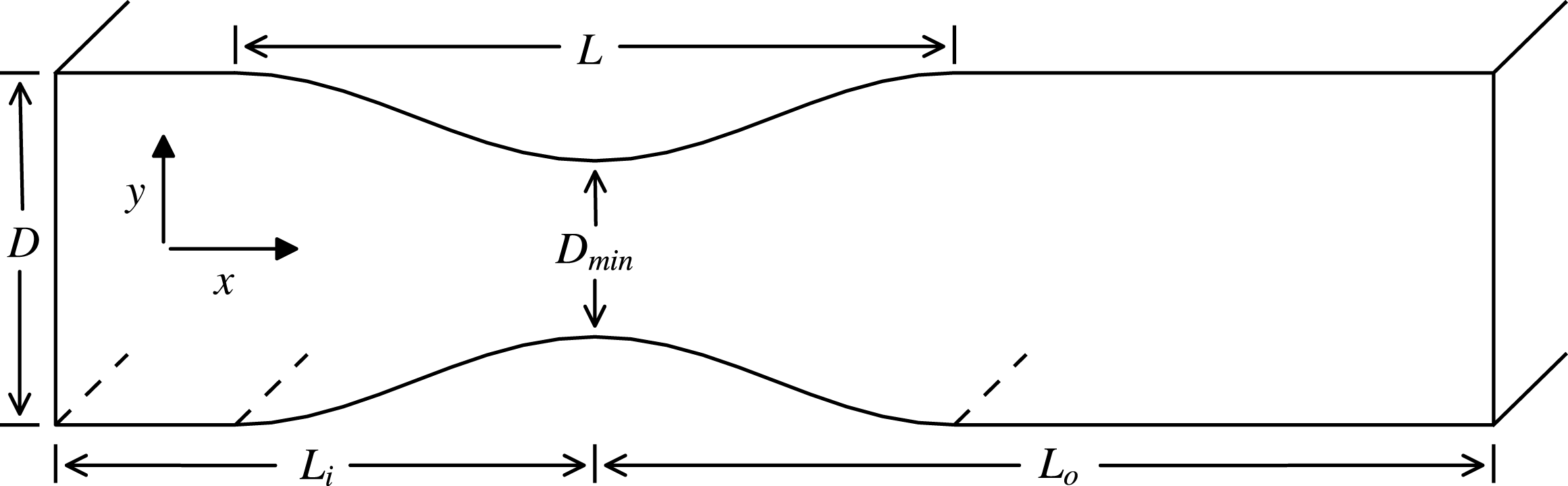
The constricted channel geometry as well as the parameters that define the geometry are shown in figure 1. We consider a rigid straight channel with a smooth constriction with 50 % occlusion. The channel has width $D$ and throat spacing $D_{min}$ . In our study, the width ratio is $D_{min}/D=0.5$ . The relative occlusion of the channel, which is defined by

(2.1)

$$\begin{eqnarray}s=1-\frac{D_{min}}{D},\end{eqnarray}$$

is therefore $s=0.5$ . Another important parameter is the stenosis length, $L$ , which is equal to $2D$ in this work. The stenosis shape is based on the work of Sherwin & Blackburn (Reference Sherwin and Blackburn2005), so that the upper and lower stenosis walls are given by

(2.2)

$$\begin{eqnarray}y(x)=\pm 0.5D_{min}\pm 0.5(D-D_{min})\sin ^{2}\left(\frac{\unicode[STIX]{x03C0}x}{L}\right)\quad (-0.5\leqslant (x/L)\leqslant 0.5),\end{eqnarray}$$

where $x$ is the streamwise coordinate measured from the narrowest point of the constriction and $y$ is the perpendicular coordinate measured from the channel centreline.

Figure 1.

Computational domain $\unicode[STIX]{x1D6FA}$ and geometric parameters which define the constricted channel geometry (not to scale).

In an ideal problem the channel domain is infinite, but in practice, the computational domain $\unicode[STIX]{x1D6FA}$ has finite inflow length $L_{i}$ and outflow length $L_{o}$ , upstream and downstream of the throat, respectively. Hence, they were made sufficiently large to allow the results to be independent of these lengths; verification tests are shown in § 4. The constricted channel is assumed homogeneous (infinite) in the spanwise direction.

The fluid is considered to be Newtonian and the Reynolds number is defined as

(2.3)

$$\begin{eqnarray}Re=\frac{\bar{u}_{m}D}{\unicode[STIX]{x1D708}},\end{eqnarray}$$

where $\bar{u}_{m}$ is the mean velocity of the fluid in an unconstricted cross-section, $D$ is the channel width and $\unicode[STIX]{x1D708}$ is the fluid’s kinematic viscosity. In this work, we investigated a range of $Re$ from 45 to 720, covering the primary and secondary global instabilities.

3 Methodology

The analysis is composed by four distinct parts. First, two-dimensional simulations of the incompressible Navier–Stokes equations are performed, in order to obtain the base flows for which the stability analyses are carried out. These simulations are time dependent, but for all the cases investigated in this paper the resulting base flows are steady. Second, linear stability analysis of the two-dimensional base flows with respect to two- and three-dimensional perturbations are carried out. The results were used to determine the critical Reynolds number, as well as the parameter space for which the flow is linearly stable. Afterwards, nonlinear numerical simulations are employed to characterize the bifurcation. The fourth part consists of computing the optimal growths in linearly stable conditions of the base flows. The maximum energy growth is obtained for different Reynolds numbers and spanwise wavenumbers, but dependence on spanwise wavenumber was only established for the asymmetric flow. Beside this, the convective mechanisms which led to the local maximum growth are investigated. This approach is applied for Reynolds numbers lower than the critical ones for the primary and secondary global instabilities in the constricted channel flow. In addition, a section about the nonlinear effects of optimal initial perturbations which have huge energy amplification for the asymmetric base flow is presented and the physical mechanism for the transition process of the secondary instability is discussed.

3.1 Two-dimensional base flow calculation

The fluid motion is governed by the incompressible Navier–Stokes equations, written in non-dimensional form using the channel width $D$ as the reference length, the fluid density $\unicode[STIX]{x1D70C}$ as the reference density and the mean velocity $\bar{u}_{m}$ as the reference speed:

(3.1)

$$\begin{eqnarray}\unicode[STIX]{x2202}_{t}\boldsymbol{u}=-(\boldsymbol{u}\boldsymbol{\cdot }\unicode[STIX]{x1D735})\boldsymbol{u}-\unicode[STIX]{x1D735}p+Re^{-1}\unicode[STIX]{x1D6FB}^{2}\boldsymbol{u},\quad \text{with }\unicode[STIX]{x1D735}\boldsymbol{\cdot }\boldsymbol{u}=0\text{ in }\unicode[STIX]{x1D6FA},\end{eqnarray}$$

where $\unicode[STIX]{x2202}_{t}$ denote a partial derivative with respect to time $t$ , $\boldsymbol{u}(\boldsymbol{x},t)=(u,v)(x,y,t)$ is the velocity vector, $p(\boldsymbol{x},t)$ is the pressure field, $Re$ is the Reynolds number and $\unicode[STIX]{x1D6FA}$ is the flow domain.

Boundary conditions were imposed on (3.1) as follows. Dirichlet boundary conditions were imposed at the inflow boundary, at the solid walls we imposed a no-slip condition, and Neumann conditions were specified at the outflow boundary. The boundary conditions are summarized as

(3.2a )

$$\begin{eqnarray}\displaystyle \boldsymbol{u}(\boldsymbol{x},t) & = & \displaystyle U_{\infty }\hat{\boldsymbol{x}}\quad \text{for }\boldsymbol{x}\in \unicode[STIX]{x2202}\unicode[STIX]{x1D6FA}_{i},\end{eqnarray}$$

(3.2b )

$$\begin{eqnarray}\displaystyle \boldsymbol{u}(\boldsymbol{x},t) & = & \displaystyle \mathbf{0}\quad \text{for }\boldsymbol{x}\in \unicode[STIX]{x2202}\unicode[STIX]{x1D6FA}_{w},\end{eqnarray}$$

(3.2c,d )

$$\begin{eqnarray}\unicode[STIX]{x2202}_{x}\boldsymbol{u}(\boldsymbol{x},t)=\mathbf{0},\quad p(\boldsymbol{x},t)=0\quad \text{for }\boldsymbol{x}\in \unicode[STIX]{x2202}\unicode[STIX]{x1D6FA}_{o},\end{eqnarray}$$

where $\unicode[STIX]{x1D6FA}_{i}$ is the inflow boundary, $\unicode[STIX]{x1D6FA}_{w}$ is the solid walls and $\unicode[STIX]{x1D6FA}_{o}$ is the outflow boundary, and $U_{\infty }=1.0$ is the inlet velocity. Furthermore, for the symmetric flow, a slip condition was imposed at the centreline of the channel, so as to ensure that the flow is symmetrically ejected from the throat. At the inflow and centreline boundaries and walls we imposed a high-order pressure boundary condition as described in Karniadakis, Israeli & Orszag (Reference Karniadakis, Israeli and Orszag1991).

The mathematical formulation and computational implementation of the normal and non-normal stability analyses are given in the Appendix.

3.2 Nonlinear analysis

Knowing the linear stability analysis we can estimate the onset of instabilities, and variables such as the critical Reynolds number, wavelength and unstable mode topology can be determined. However, the understanding of instability mechanisms that play a key role after the onset of the transitions are beyond the scope of this theory. Thus, fully three-dimensional simulations are performed, in order to take the nonlinear effects into account, which can guide us to comprehend the instability mechanisms and classify the bifurcations. Besides that, optimal initial perturbations from transient growth, which have huge energy amplification in hysteretic regions, can lead the initial disturbance to nonlinear saturation. If it happens, a subcritical nonlinear saturation could occur for Reynolds numbers lower than the critical, so that the nonlinear three-dimensional calculations allowed us to assess it. Therefore, the nonlinear analysis will highlight the main features of the bifurcations and nonlinear effects of steady flows in the constricted channel.

For the nonlinear calculations we used the same approach as outlined in § 3.1. However, a Fourier expansion was applied in the discretization in the spanwise direction (Karniadakis Reference Karniadakis1990) and the simulations were carried out with 4 or 8 Fourier modes (8 or 16 planes of data in the spanwise direction). In addition, we did not use a slip condition in the channel centreline for the three-dimensional simulations of the symmetric flow, so when the jet goes through the constriction it is allowed to deflect.

In order to evaluate the evolution of small perturbations of unstable modes or optimal initial perturbations as discussed above, the dimensionless amount of flow kinetic energy in each spanwise Fourier mode $k$ is

(3.4)

$$\begin{eqnarray}E_{k}=\frac{1}{2A\bar{u}_{m}^{2}}\int _{A}\hat{\boldsymbol{u}}_{k}\boldsymbol{\cdot }\hat{\boldsymbol{u}}_{k}^{\ast }\,\text{d}A,\end{eqnarray}$$

where $\hat{\boldsymbol{u}}_{k}^{\ast }$ is the complex conjugate of the velocity data in the $k$ th Fourier mode and $A$ is the two-dimensional cross-section of the domain being considered.

4 Numerical approach

The spectral/hp element method was used for spatial discretization of the plane geometry (Karniadakis & Sherwin Reference Karniadakis and Sherwin2005), coupled with a Fourier decomposition in the spanwise direction. Figure 2 shows a close-up of the computational mesh around the throat used for the present analysis. The refined discretization by quadrilateral elements around the throat was based on the mesh of the work of Sherwin & Blackburn (Reference Sherwin and Blackburn2005). The computational mesh was composed by 2974 spectral elements, with 2932 quadrilateral and 42 triangular. The inflow and outflow lengths were $30D$ and $75D$ from the throat of the stenosis. A domain this long is necessary to accommodate well the disturbance upstream and downstream during the transient growth and linear stability analysis.

Figure 2.

Close-up of the computational mesh around the throat; the dimension is given in terms of channel height $D$ . The mesh has 2974 spectral elements.

Table 1.

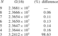
Convergence of the two-dimensional optimal growth at $\unicode[STIX]{x1D70F}=16$ for $Re=720$ with respect to the variation of the spectral element polynomial order $N$ , computed with $M_{1}$ .

To calculate the base flows, the equations (3.1) were solved in two dimensions using a stiffly stable splitting scheme (Karniadakis et al. Reference Karniadakis, Israeli and Orszag1991). Time integration was carried out using second-order velocity-correction schemes with value of the non-dimensional time step of 0.001 and 0.0005 for the higher polynomial order. For all stability calculations, a Krylov subspace of dimension of $20$ was used and in both methods the eigensolution convergence parameter was set to $10^{-5}$ .

The two-dimensional maximum energy growth for the highest Reynolds number evaluated in this paper occurs around $\unicode[STIX]{x1D70F}=16$ for $Re=720$ . Thus, we used these parameters to analyse the mesh convergence in the most challenging case simulated here. Table 1 shows the convergence of the two-dimensional optimal growth with respect to the polynomial order, using the mesh $M_{1}$ , which is the mesh adopted in this work (table 2). It can be seen that, even for fourth-order polynomials (i.e. fifth-order accuracy in space) the convergence is reached with uncertainty less than 0.2 %. Therefore, the base flows and the stability analyses for the symmetric and asymmetric flows were computed with $N=6$ . However, the fully three-dimensional simulations of the nonlinear analysis were performed with $N=5$ . 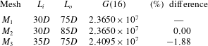Table 2 depicts the convergence of the two-dimensional optimal growth with respect to the inflow and outflow lengths, using $N=6$ . It can be seen that there is no change in the optimal growth when the outflow length is varied. However, a longer inflow length is responsible for a small variation in the optimal growth, so that it produced a numerical error which is considered acceptable for the worst case.

Figure 3.

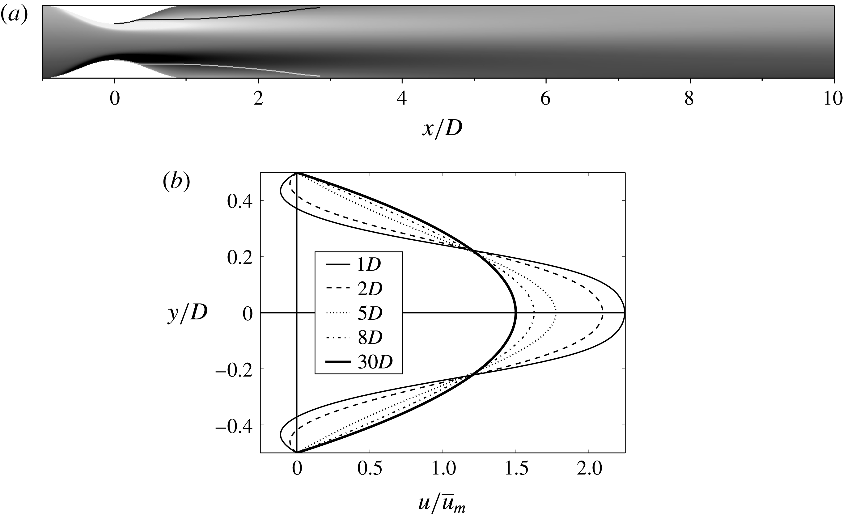
Two-dimensional base flow close to primary instability at $Re=270$ . (a) Vorticity contours and streamlines showing the recirculating regions. (b) Velocity profiles. Reattachment occurs at $x/D=2.82$ .

Table 2.

Convergence of the two-dimensional optimal growth at $\unicode[STIX]{x1D70F}=16$ for $Re=720$ with respect to the variation of the inflow and outflow lengths, computed with polynomial order $N=6$ .

5 Primary global instability

5.1 Base flow characteristics

The two-dimensional base flow features close to the primary instability are shown in figure 3, which illustrates vorticity contours, streamlines and velocity profiles for the symmetric flow at $Re=270$ . It can be seen that, in figure 3(a), the flow is symmetric when it goes through the throat with flow separation downstream of the narrowest section. After that, it expands and reattaches on the upper and lower walls of the channel. The flow ejected from the throat, which has strong vorticity, establishes two recirculating regions at each side of the channel, and shear layers that extend downstream to nearly $x/D=2.82$ . Figure 3(b) shows velocity profiles of the $x$ -velocity along the channel height position for five different locations downstream from the throat. As expected by a constricted channel with $50\,\%$ occlusion, the maximum $x$ -velocity is higher than $2\bar{u}_{m}$ close to the throat, easily observed in the profile velocity at $x/D=1$ . The thicker solid line represents the velocity profile at $x/D=30$ (inflow length) from the throat, so that at this point the flow is fully re-established, with the maximum velocity differing only $0.01\,\%$ from its asymptotic value of $3/2U_{\infty }$ . Hence, the inflow length is acceptable for the development of the flow in the channel.

Figure 4.

Linear stability analysis for the primary instability. (a) Plot of the leading eigenvalues, $\unicode[STIX]{x1D70E}$ , against spanwise wavenumber $\unicode[STIX]{x1D6FD}$ for different Reynolds numbers. Inset: the critical Reynolds number for $\unicode[STIX]{x1D6FD}=0$ is $Re=281.2$ , determined by interpolation. (b) Neutral stability curve for the symmetric steady flow in the constricted channel. In the region on the right-hand side of the curve (dark region) the two-dimensional flow is linearly unstable to infinitesimal three-dimensional perturbation. The critical Reynolds number is $Re_{c}=278.8$ .

5.2 Normal stability analysis

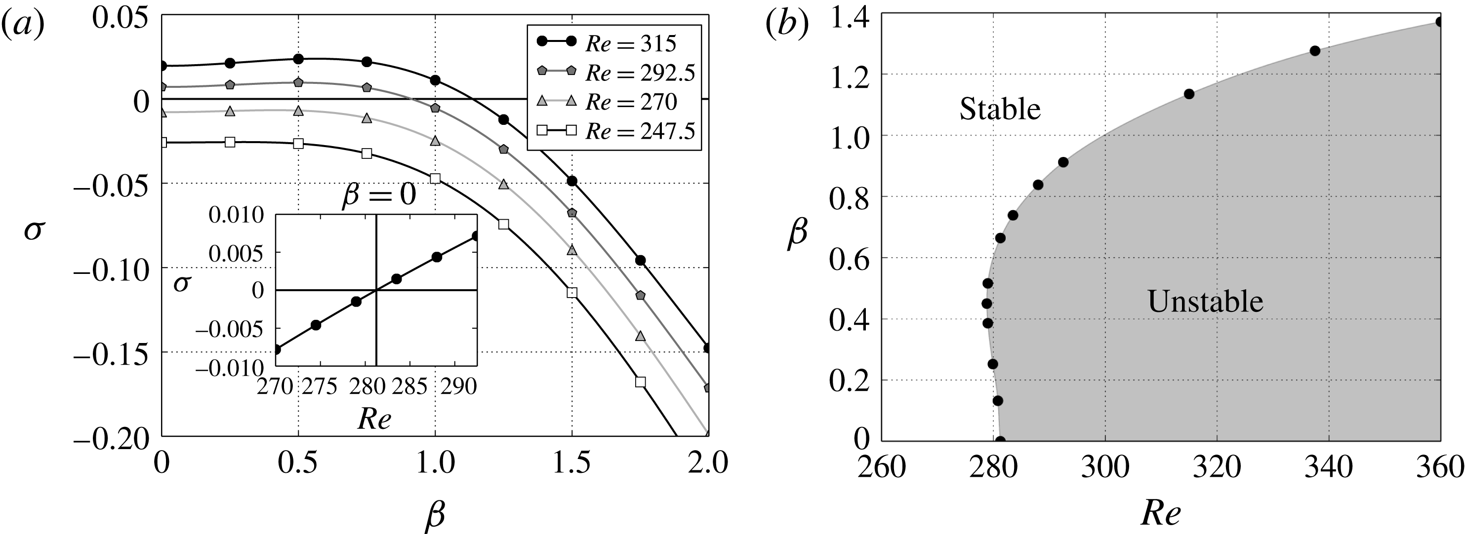
In order to investigate the primary instability and to determine the unstable regions of the symmetric flow, the first step was to carry out a normal stability analysis. Figure 4(a) shows the leading eigenvalues, $\unicode[STIX]{x1D70E}$ , as a function of spanwise wavenumber $\unicode[STIX]{x1D6FD}$ for four different Reynolds numbers. All leading eigenvalues found were real and only one unstable mode was revealed in the Reynolds number range considered. The inset in figure 4(a) shows the leading eigenvalues, $\unicode[STIX]{x1D70E}$ , as a function of Reynolds number for $\unicode[STIX]{x1D6FD}=0$ . The critical Reynolds number for two-dimensional disturbance is $281.2$ , determined by interpolation with uncertainty of less than $1\,\%$ . Figure 4(b) shows the neutral stability curve for the primary instability in the constricted channel for Reynolds numbers up to 360. Everywhere to the right-hand side of the curve (dark region) the two-dimensional flow is linearly unstable to infinitesimal perturbations, so that the curve which separates the light and dark regions represents the parameter space for which the base flow is neutrally stable. The symmetric flow first becomes unstable for a three-dimensional perturbation and the unstable region quickly extends to a wide range of spanwise wavenumbers, but the Reynolds number for which the flow is unstable with respect to a two-dimensional perturbation is only slightly higher. The critical Reynolds number and corresponding spanwise wavenumber are $Re_{c}=278.8\pm 0.1$ and $\unicode[STIX]{x1D6FD}_{c}=0.45\pm 0.01$ . The critical spanwise wavelength is $2\unicode[STIX]{x03C0}/\unicode[STIX]{x1D6FD}_{c}=13.96$ channel widths. Pitt (Reference Pitt2005) reported the onset of the primary instability at $Re=278.5$ for $\unicode[STIX]{x1D6FD}=0.45$ , which agrees with our value. Hence, the simulations parameters and mesh setup were considered to be properly chosen.

Figure 5.

(a) Energy diagram of the symmetric steady flow for $\unicode[STIX]{x1D6FD}=0.45$ . The diagram was built with the energy of the two-dimensional component of the Fourier modes ( $k=0$ ). (b) Velocity contours perpendicular to the $x$ -direction of the three-dimensional flow at $Re=270$ , when it achieves nonlinear saturation of the two-dimension Fourier mode.

Pitt (Reference Pitt2005) investigated the stability of the flow inside a $60\,\%$ constricted channel with critical Reynolds number at $Re=127.4$ and critical spanwise wavenumber of $\unicode[STIX]{x1D6FD}=0.55$ . This suggests that the narrower the constriction the lower the Reynolds number required for primary instability. On the other hand, the critical spanwise wavenumber is higher than in the case with $50\,\%$ occlusion. Sherwin & Blackburn (Reference Sherwin and Blackburn2005), in a 75 % constricted tube with the same stenotic shape as employed in this study, found a critical Reynolds number of $Re=722$ for steady flow. Griffith et al. (Reference Griffith, Leweke, Thompson and Hourigan2008) analysed a tube for different stenosis degrees and observed a critical Reynolds number not exceeding 395 for the highest stenosis degree.

5.3 Nonlinear characterization of the bifurcation

Having established the critical values of the primary instability, the next step of our analysis consisted of understanding the mechanisms by which the bifurcation occurs, thus fully nonlinear three-dimensional simulations were performed around the primary instability. The simulations were initialized with the nonlinear saturation of the unstable base flow at $Re=360$ with all Fourier modes saturated; however, when the Reynolds number was lower than $324$ the three-dimensional ( $\unicode[STIX]{x1D6FD}>0$ ) Fourier modes went to zero, regardless of whether the base flow was seeded with the most unstable mode from linear stability analysis or with nonlinear saturation of a unstable base flow, although for higher Reynolds number the three-dimensionalities held for longer times. 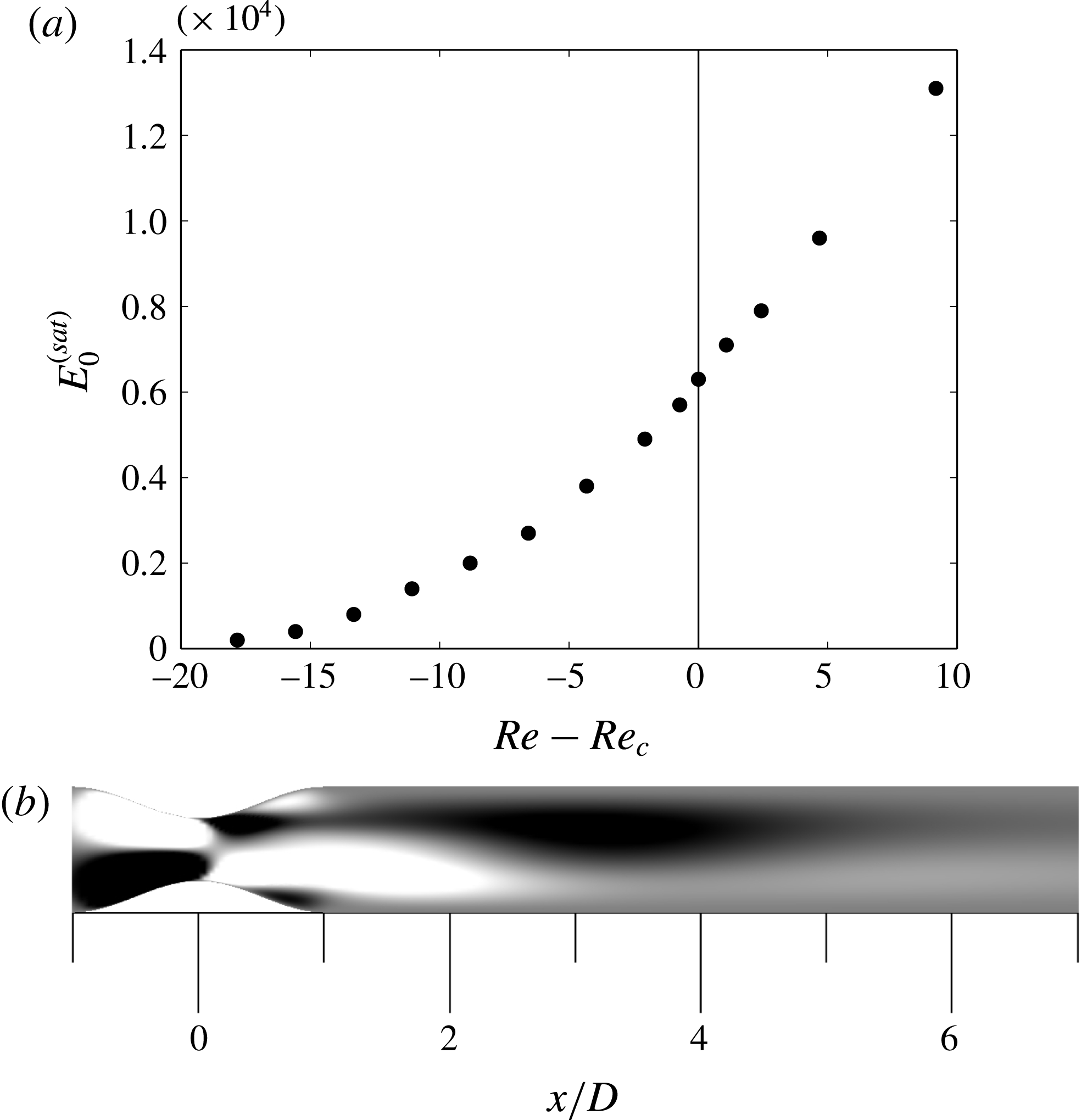The two-dimensional ( $\unicode[STIX]{x1D6FD}=0$ ) mode, however, presented growth and saturation, modifying the base flow and giving rise to an asymmetric flow field. Figure 5(a) shows a diagram that was built with the energy of the two-dimensional component of the Fourier modes ( $k=0$ ); the solid circles in the diagram denote the energy that was transferred from the base flow to the two-dimensional mode.

In order to investigate further this somewhat unexpected behaviour, additional calculations were carried out. For three-dimensional simulations any perturbation at Reynolds number in the hysteretic region, such as white noise, no matter how small, was enough to lead the flow from symmetric to asymmetric, breaking the symmetry of the system (figure 5 b). In other words, any perturbation in the symmetric base flow for Reynolds number higher than 260 raised the initial energy up to the hysteretic curve in the three-dimensional nonlinear simulations. However, it is remarkable that the two-dimensional base flows calculated without the constraint in the centreline of the channel (slip condition) were perfectly symmetric even if they were calculated very close to the critical Reynolds number (approaching from lower $Re$ ).

As a final attempt to evaluate the transition and verify if it had a fundamental three-dimensional character, although resulting in a two-dimensional flow, two-dimensional simulations at Reynolds numbers in the hysteretic region were initialized with the mode $0$ (i.e. spanwise-averaged field) from the three-dimensional unstable base flow at $Re=360$ , which is an asymmetric flow field. It was observed that the asymmetric flow became symmetric with time until it was fully re-established. Seeing that, we concluded that the bifurcation is triggered by a three-dimensional mechanism, and the three-dimensional unstable modes transfer energy to the two-dimensional (asymmetric) mode due to nonlinear interactions.

5.4 Non-normal stability analysis

From the linear stability analysis, we have established the critical Reynolds number, as well as the region where the flow is linearly unstable to infinitesimal two- and three-dimensional perturbations in the range of Reynolds numbers considered. Now we turn to the examination of the convective mechanisms and the largest transient energy growth for a given optimal initial perturbation as well as the behaviour of the maximum energy growth with Reynolds number and time.

5.4.1 Dependence on Reynolds number

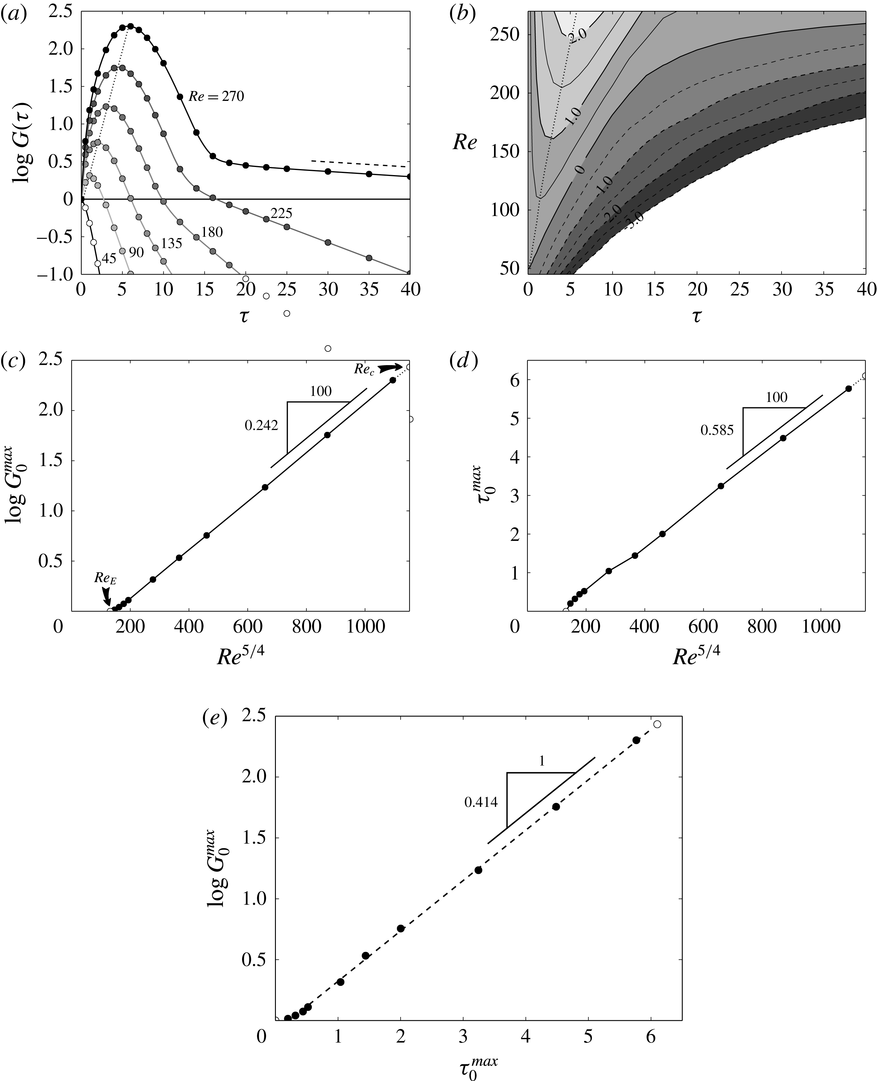
Figure 6 summarizes the optimal energy growth for two-dimensional perturbations before the primary instability. Figure 6(a) shows the optimal envelopes, $G(\unicode[STIX]{x1D70F})$ , as a function of time horizon for Reynolds numbers from $45$ up to $270$ . We recall, just to be clear, that each point in figure 6(a) corresponds to the energy growth of the optimal initial condition for a specific time $\unicode[STIX]{x1D70F}$ . So, the maximum energy growth among all optimal initial perturbations is $G_{0}^{max}(270)=2.01\times 10^{2}$ at $\unicode[STIX]{x1D70F}_{0}^{max}=5.77$ . It can be seen that all energy growth curves end up with an exponential decrease after the maximum growth; however, there is no growth at $Re=45$ for any time interval. In addition, the dashed line represents the exponential decrease associated with the leading eigenmode, $\unicode[STIX]{x1D70E}$ , of the normal analysis, which match the transient growth exponential decrease at long times.

Figure 6.

Dependence on Reynolds number of the two-dimensional transient energy growth before primary instability. (a) Energy growth envelopes, $G(\unicode[STIX]{x1D70F})$ , as a function of $\unicode[STIX]{x1D70F}$ for Reynolds number varying from 45 up to 270. The dashed line represents the exponential decrease associated with the leading eigenmode. (b) Logarithmic contours for two-dimensional optimal energy growth, $G(\unicode[STIX]{x1D70F},Re)$ , as a function of $\unicode[STIX]{x1D70F}$ and $Re$ . The critical Reynolds number for the first growth is $Re_{E}=49.5$ . The dotted-line curve shows the local of maximum energy growth as a function of $\unicode[STIX]{x1D70F}$ . Variation of maximum (c) growth and (d) time as a function of $Re^{5/4}$ . Values of $\log G_{0}^{max}$ and $\unicode[STIX]{x1D70F}_{0}^{max}$ increase linearly with $Re^{5/4}$ . (e) Maximum energy growth as a function of time of maximum growth for the Reynolds number range from $Re_{E}$ to $Re_{c}$ . The value of $\log G_{0}^{max}$ grows linearly with $\unicode[STIX]{x1D70F}_{0}^{max}$ .

Optimal growth logarithmic contours in the $(\unicode[STIX]{x1D70F},Re)$ plane are shown in figure 6(b). The solid and dashed lines represent regions with $G\geqslant 1$ and $G<1$ , respectively. So, in the lighter regions above the line where $\log G=0$ the optimal growth is larger than unity. In addition, the dotted line, in figure 6(a,b), shows the local of maximum growth as a function of $\unicode[STIX]{x1D70F}$ . From these data, an important observation can be made: the critical Reynolds number, $Re_{E}$ , for which the energy growth first exceeds unity is obtained when $\unicode[STIX]{x2202}G(\unicode[STIX]{x1D70F},Re_{E})/\unicode[STIX]{x2202}\unicode[STIX]{x1D70F}|_{\unicode[STIX]{x1D70F}=0}=0$ , in other words, this happens when the line $\log G=0$ intercept the $Re$ -axis as shown in figure 6(b). The critical value for the smallest growth is $Re_{E}=49.5$ for two-dimensional perturbations, so this value is lower than that found in a backward-facing step (Blackburn et al. Reference Blackburn, Barkley and Sherwin2008a ; Cantwell et al. Reference Cantwell, Barkley and Blackburn2010). This means that perturbations at Reynolds numbers below $Re_{E}$ will decrease monotonically. It should be also noted that, in figure 6(a), the optimal growth curve at $Re=90$ has a positive slope at $\unicode[STIX]{x1D70F}=0$ ; on the other hand, at $Re=45$ the curve decreases monotonically.

Figure 6(c,d) shows the variation of maximum growth and time of maximum growth as a function of $Re^{5/4}$ . The open circles represent the critical Reynolds numbers $Re_{E}$ and $Re_{c}$ for the two-dimensional analysis as indicated in figure 6(c). It is evident that the $\log G_{0}^{max}$ and $\unicode[STIX]{x1D70F}_{0}^{max}$ increase linearly with $Re^{5/4}$ . We found the expressions

(5.1)

$$\begin{eqnarray}\log G_{0}^{max}\simeq 2.42\times 10^{-3}Re^{5/4}\end{eqnarray}$$

and

(5.2)

$$\begin{eqnarray}\unicode[STIX]{x1D70F}_{0}^{max}\simeq 5.85\times 10^{-3}Re^{5/4}.\end{eqnarray}$$

These expressions are valid between $Re_{E}$ and $Re_{c}$ , in other words, they are acceptable from the Reynolds number for which there is the first smallest growth to the critical Reynolds number of the primary instability. Above $Re_{c}$ , $G_{0}^{max}$ diverges because the flow becomes linearly unstable. Notice that the critical values of $G_{0}^{max}$ and $\unicode[STIX]{x1D70F}_{0}^{max}$ were calculated by extrapolation of (5.1) and (5.2), respectively. Thus, the critical maximum growth is $G_{0}^{max}(Re_{c})\approx 2.71\times 10^{2}$ and the corresponding critical time of maximum growth is $\unicode[STIX]{x1D70F}_{0}^{max}(Re_{c})\approx 6.10$ . Similar exponential maximum growths were observed for other separated flows in confined and unconfined geometries; however, they do not obey the dependence with $Re^{5/4}$ . A linear dependence with Reynolds number has been found in many studies: in a backward-facing step (Blackburn et al. Reference Blackburn, Barkley and Sherwin2008a ), steady flow in a stenotic pipe (Blackburn et al. Reference Blackburn, Sherwin and Barkley2008b ) and in an axisymmetric pipe with a sudden expansion (Cantwell et al. Reference Cantwell, Barkley and Blackburn2010). However, Cantwell & Barkley (Reference Cantwell and Barkley2010) reported square dependence in a flow past a circular cylinder in the subcritical regime. Even more notably, Sheard & Blackburn (Reference Sheard and Blackburn2010) found linear maximum growth for two regions with different power-law dependencies in a steady flow through an axisymmetric aneurysm model, so that the first region had a dependence of $Re^{9/5}$ and the second of $Re^{7/5}$ . It is worth noting that the maximum energy growth for the confined flows cited above do not present the same Reynolds dependence as classical planar Couette flow (Reddy & Henningson Reference Reddy and Henningson1993) and the Hagen–Poiseuille flow (Schmid & Henningson Reference Schmid and Henningson1994); they both reveal maximum growth dependence with $Re^{2}$ .

The $\log G_{0}^{max}$ is plotted in figure 6(e) as a function of $\unicode[STIX]{x1D70F}_{0}^{max}$ . As expected from figure 6(c,d), $\log G_{0}^{max}$ grows linearly with $\unicode[STIX]{x1D70F}_{0}^{max}$ . From (5.1) and (5.2) we obtain

(5.3)

$$\begin{eqnarray}\log G_{0}^{max}\simeq 0.414\unicode[STIX]{x1D70F}_{0}^{max}.\end{eqnarray}$$

We can draw two important conclusions. First, the energy growths for the Reynolds number range from the first smallest growth slightly above $Re_{E}$ to the critical value $Re_{c}$ reach their maxima with the same growth rate. Secondly, it should be noted that, since they have the same growth rate, the optimal initial perturbations travel through the channel and reach the peak growth at different positions downstream from the throat; the farther from the throat the higher the Reynolds number, such that the perturbation velocity profile is similar at their peak growth. This behaviour was also observed in a stenotic pipe by Griffith et al. (Reference Griffith, Leweke, Thompson and Hourigan2008), however it was explained by the existence of self-similarity, which could be extended for constricted channel geometries.

Figure 7.

Plots of two-dimensional logarithmic contours of energy before primary instability, computed at $Re=270$ . (a) Optimal initial perturbation for $\unicode[STIX]{x1D70F}=6$ . (b) Optimal perturbation growth outcome at $\unicode[STIX]{x1D70F}=6$ . The vectors represent the velocity field.

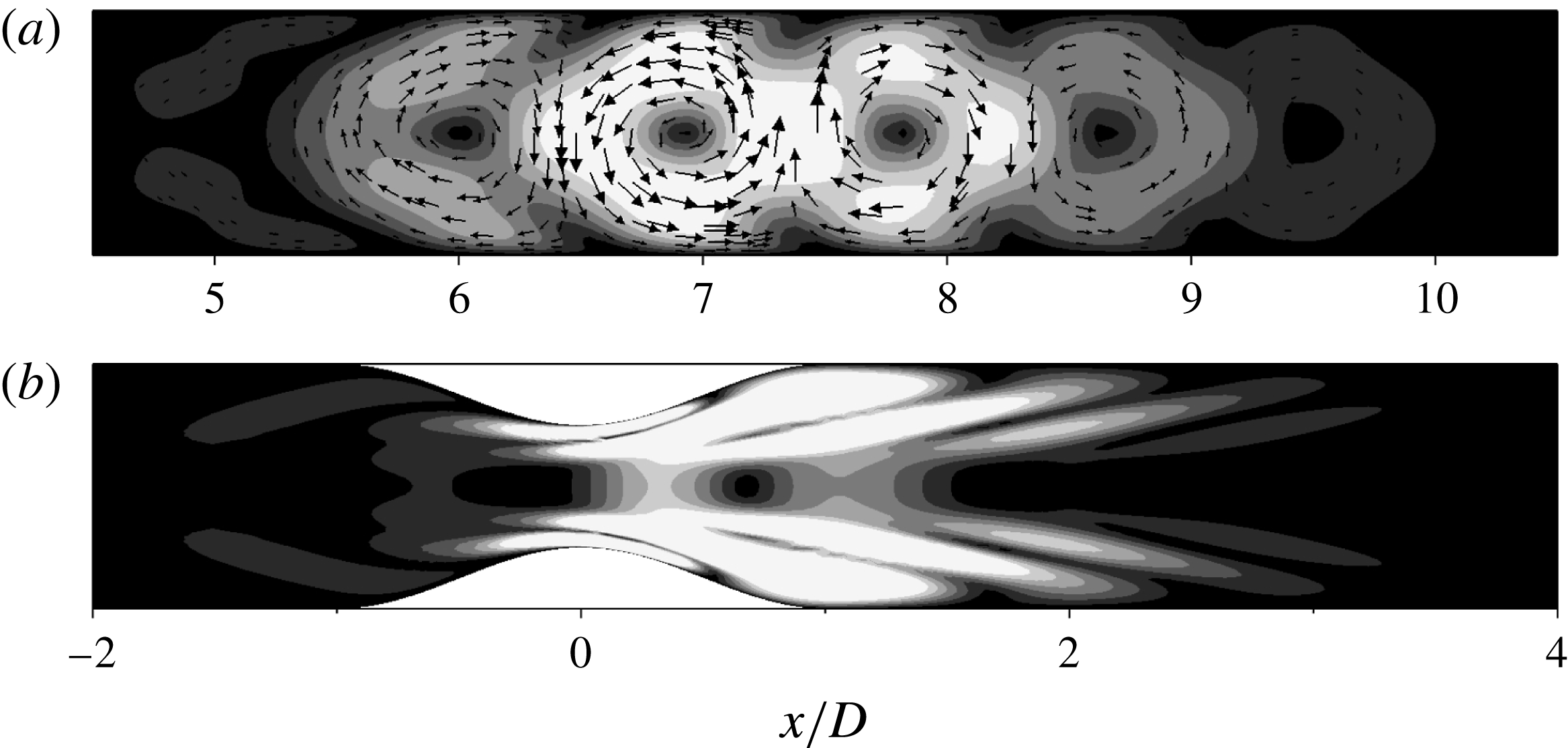
In order to comprehend the structure of the perturbation for the most amplified case at $Re=270$ , figure 7 shows the logarithmic contours of energy for $\unicode[STIX]{x1D6FD}=0$ . Optimal initial perturbation for $\unicode[STIX]{x1D70F}=6$ is shown in figure 7(a). Most of the initial disturbance is concentrated at the shear layer in the constriction and around the separated flow; however, there is also a mild energy upstream of the constriction. In addition, the perturbation exhibits chevron-shaped contours upstream of the constriction as well as in the shear layers, featuring a sinuous disturbance. This sinuous initial disturbance around the shear layer was also observed in other shear flows (Blackburn et al. Reference Blackburn, Barkley and Sherwin2008a ,Reference Blackburn, Sherwin and Barkley b ; Cantwell et al. Reference Cantwell, Barkley and Blackburn2010; Griffith et al. Reference Griffith, Thompson, Leweke and Hourigan2010). Figure 7(b) illustrates the optimal perturbation at $\unicode[STIX]{x1D70F}=6$ corresponding to the initial condition shown in figure 7(a). The evolution of the optimal perturbation is a wave packet, which becomes a series of spanwise counter-rotating rolls as emphasized by the velocity field vectors. Moreover, the minimal energy is located in the centre of the rollers, and advected downstream following the centreline of the channel. The evolution of shear layers giving rise to spanwise counter-rotating rolls was also obtained in a backward-facing step (Blackburn et al. Reference Blackburn, Barkley and Sherwin2008a ) and in two-dimensional plane Couette and Poiseuille flows (Farrell Reference Farrell1988).

6 Secondary global instability

6.1 Base flow characteristics

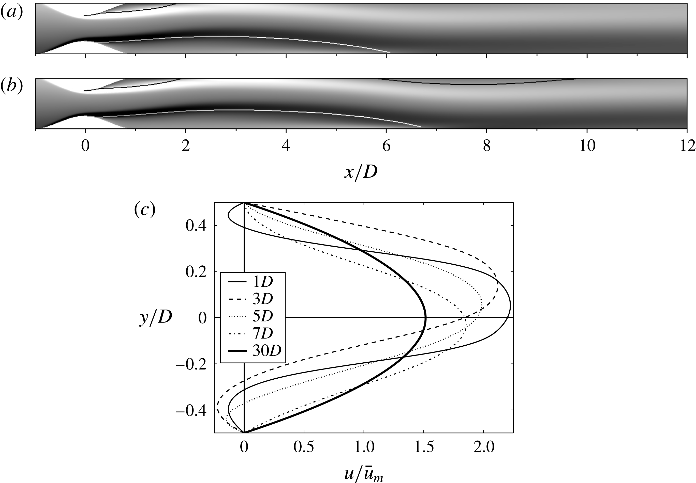
Now we turn our attention to the secondary global instability. The main characteristics of the two-dimensional base flow close to the secondary instability are shown in figure 8. In this figure we present the vorticity contours, streamlines and velocity profiles along the streamwise direction of the channel. It is remarkable that, as previously discussed, the base flow is asymmetric when the flow is ejected from the throat (figure 8 a). The two boundary layers in the constriction separate immediately after the narrowest section and turn upward. The streamlines clearly exhibit the upward deflection of the jet and the recirculating regions of different size in the flow, so that, at $Re=540$ , the reattachments on the channel walls occur at two different points. The first streamline on the top reattaches at $x/D=1.82$ and the second on the bottom at $x/D=6.04$ . If we increase the Reynolds number a third recirculating region appears at the upper wall as shown in figure 8(b). Velocity profiles of the $x$ -velocity as a function of the channel height from the central plane for $x/D=$ 1, 3, 5, 11 and 30 at $Re=540$ are shown in figure 8(c). Two aspects are noteworthy about these velocity profiles. The first is that, when the asymmetric flow is deflected upwards, we can easily see the start of the deviation on $y$ -direction at $x/D=1$ ; afterwards it reaches its maximum $y$ -position near $x/D=3$ . The second, which is not evident in the flow visualization, is that the flow deflects downwards, reaching its maximum deviation approximately at $x/D=7$ . After that the flow goes back to the central position and tends to the Poiseuille solution. At $x/D=30$ , as previously mentioned at $Re=270$ , the Poiseuille flow is re-established, but with a difference of approximately of $1\,\%$ from its asymptotic value.

Figure 8.

Two-dimensional base flow close to secondary instability. Vorticity contours and streamlines, showing the recirculating regions at (a) $Re=540$ and (b) $Re=720$ . (c) Velocity profiles at $Re=540$ . Reattachments occur at $x/D=1.82$ and $x/D=6.04$ for $Re=540$ .

6.2 Normal stability analysis

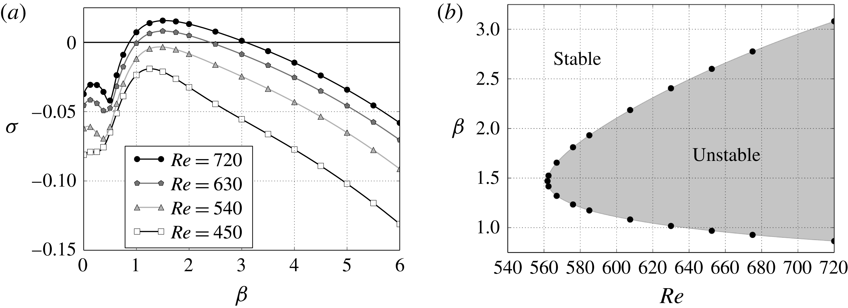
Following the same discussion from the primary instability, figure 9 shows the normal stability analysis of the two-dimensional base flow after the base flow symmetry breaking. Figure 9(a) shows leading eigenvalues against spanwise wavenumber for four different Reynolds numbers. It is possible to identify one unstable mode for this range of Reynolds number; however, a second mode is rising for smaller spanwise wavenumber, being evident at $Re=720$ . This suggests that for higher Reynolds numbers it will become a second unstable mode. From this plot, we note that the spanwise wavenumber of the most unstable eigenvalues in each Reynolds number is around $\unicode[STIX]{x1D6FD}=1.5$ . In addition, all leading eigenvalues obtained are real, as previously observed for the primary instability, except for $\unicode[STIX]{x1D6FD}=0.5$ at $Re=720$ , which appears to be a discontinuity in the curve. Figure 9(b) shows the neutral stability curve for the secondary instability in the constricted channel up to $Re=720$ . The asymmetric flow firstly becomes unstable for a three-dimensional perturbation. The critical Reynolds number and corresponding spanwise wavenumber are $Re_{c}=562.0\pm 0.1$ and $\unicode[STIX]{x1D6FD}_{c}=1.47\pm 0.01$ . The critical spanwise wavelength is $2\unicode[STIX]{x03C0}/\unicode[STIX]{x1D6FD}_{c}=4.27$ channel widths.

The critical Reynolds number and spanwise wavenumber for a $60\,\%$ constricted channel are approximately $290$ and $1.6$ for the secondary instability (Pitt et al. Reference Pitt, Sherwin and Theofilis2004), respectively. As previously seen for the primary instability, the critical Reynolds number is lower and the critical spanwise wavenumber is higher than in a 50 % constricted channel. These results were also found in a flow through a partially blocked channel (Griffith et al. Reference Griffith, Leweke, Hourigan and Anderson2007). Therefore, it suggests that the narrower constriction the lower critical Reynolds number and the higher critical spanwise wavenumber for the transition of the primary and secondary instability.

Figure 9.

Linear stability analysis for the secondary instability. (a) Plot of the leading eigenvalues, $\unicode[STIX]{x1D70E}$ , against spanwise wavenumber $\unicode[STIX]{x1D6FD}$ for different Reynolds numbers. (b) Neutral stability curve for the asymmetric steady flow in the constricted channel. In the region on the right hand side of the curve (dark region) the two-dimensional flow is unstable to infinitesimal three-dimensional perturbation. The critical Reynolds number is $Re_{c}=562.0$ .

6.3 Nonlinear characterization of the bifurcation

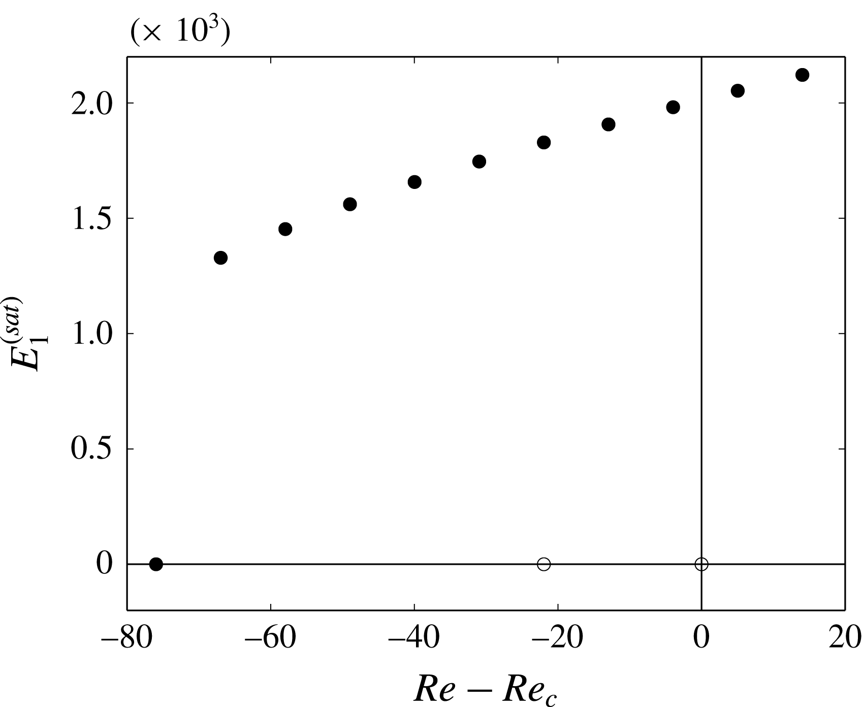
Once we found the neutral stability curve for the asymmetric flow, we proceeded with the nonlinear analysis, in order to classify the bifurcation observed. Figure 10 shows the bifurcation diagram of the asymmetric steady flow for $\unicode[STIX]{x1D6FD}=1.47$ , in which the energy was extracted from the first mode number ( $k=1$ ). The fully three-dimensional simulations were carried out with two different types of initial conditions. In the first, the initial conditions were a linear combination of the base flow and the most unstable eigenmode taken from linear stability analysis, which was multiplied by a factor small enough to make the initial growth linear, being marked by hollow circles. The second, shown by the solid circles, were the nonlinear saturation of the unstable base flow at $Re=720$ . It is evident from this diagram that the bifurcation exhibits subcritical behaviour, but with some remarkable differences from what was observed for the primary bifurcation. The hysteresis in the vicinity of the critical point can easily be seen in figure 10, and extends far away from the critical point, achieving $Re=495$ . Afterwards, the kinetic energy of the spanwise Fourier modes has a sudden fall and goes to zero.

Another important finding related to subcritical bifurcation in confined flows was reported by Sherwin & Blackburn (Reference Sherwin and Blackburn2005), who analysed an axisymmetric stenotic tube with area reduction of 75 %. Using a fully three-dimensional simulation, they concluded that the instability was subcritical. Hysteresis was confirmed and the flow also exhibited instabilities quite far from the critical point in the nonlinear simulations. However, the analysis referred to the primary instability, rather than to the secondary instability as observed here.

We consider an asymmetric flow in a channel which has a closer relationship to our system. The primary instability in a backward-facing step was determined by Barkley et al. (Reference Barkley, Gomes and Henderson2002), having a critical Reynolds number of 748, which is higher than in the constricted channel flow. The nature of the bifurcation was defined by Rani & Sheu (Reference Rani and Sheu2006), being a supercritical Hopf bifurcation. Therefore, even though the constricted channel and the backward-facing step are both flows confined by parallel walls, the way the flow bifurcates is strongly influenced by the shear layers when the flow separates.

Figure 10.

Diagram of the subcritical bifurcation of the asymmetric steady flow for $\unicode[STIX]{x1D6FD}=1.47$ . The solid circles represent the DNS seeded with the nonlinear saturation of the unstable base flow at $Re=720$ and the hollow circles with a linear combination of the base flow and the leading eigenmode.

6.4 Non-normal stability analysis

As previously done for the primary global instability, in this section transient growth analysis of the asymmetric base flow is presented; however, dependence on spanwise wavenumber is also analysed.

An important aspect in this study is that, for the most part, there is only a slight difference between the two- and three-dimensional analyses. The shape of the optimal initial conditions (in the $xy$ -plane) and their evolution in time are almost the same in both cases. In addition, there is a very small range of spanwise wavenumber for which the three-dimensional peak growth is slightly higher than in the two-dimensional case, as reported by Blackburn et al. (Reference Blackburn, Barkley and Sherwin2008a ) in a backward-facing step as well. Thereby two distinct approaches were used. First, a two-dimensional study of Reynolds number dependence is described; in other words, time horizon and Reynolds number were allowed to vary, but the spanwise wavenumber is fixed ( $\unicode[STIX]{x1D6FD}=0$ ). After that, for the three-dimensional analysis, results are presented for fixed values of Reynolds number, allowing time horizon and spanwise wavenumber to vary.

6.4.1 Dependence on Reynolds number

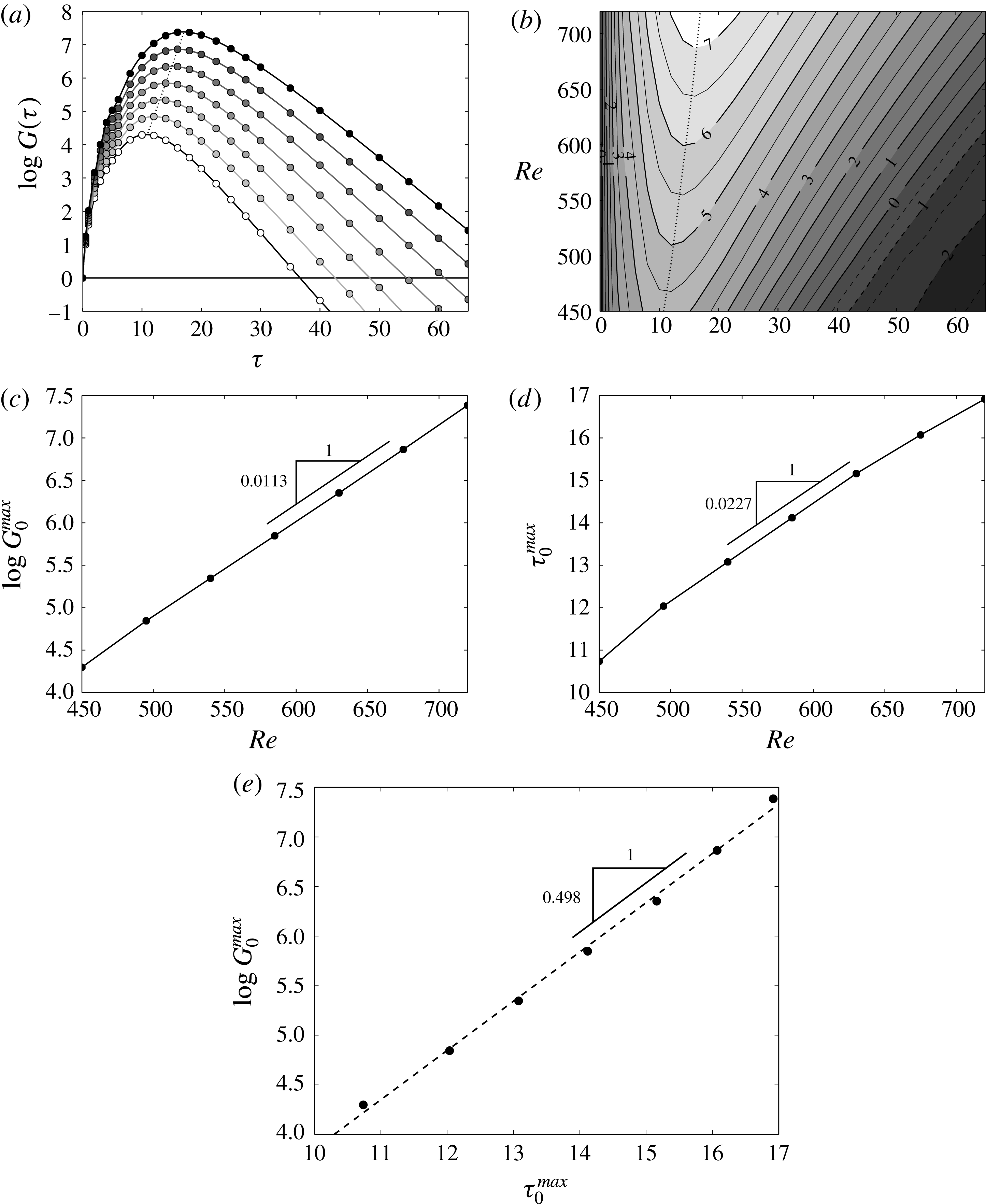
Figure 11 summarizes the optimal energy growth for two-dimensional perturbations after the primary instability. Figure 11(a) shows the optimal envelopes, $G(\unicode[STIX]{x1D70F})$ , versus time horizon for Reynolds numbers from $450$ up to $720$ . It can be seen that the optimal energy curves go directly to their maxima and decrease monotonically afterwards. The maximum energy growth among all initial perturbations is $G_{0}^{max}(720)=2.24\times 10^{7}$ at $\unicode[STIX]{x1D70F}_{0}^{max}=16.92$ . Figure 11(b) illustrates the optimal growth logarithmic contours in the $(\unicode[STIX]{x1D70F},Re)$ plane. Moreover, the dotted line in figure 11(a,b) shows the local of maximum growth as a function of $\unicode[STIX]{x1D70F}$ .

Figure 11.

Dependence on Reynolds number of the two-dimensional transient energy growth after primary instability. (a) Energy growth envelopes, $G(\unicode[STIX]{x1D70F})$ , as a function of $\unicode[STIX]{x1D70F}$ for Reynolds number varying from 450 up to 720. (b) Logarithmic contour plot for two-dimensional optimal energy growth, $G(\unicode[STIX]{x1D70F},Re)$ , as a function of $\unicode[STIX]{x1D70F}$ and $Re$ . The dotted-line curve shows the local of maximum energy growth as a function of $\unicode[STIX]{x1D70F}$ . Variation of maximum (c) growth and (d) time as a function of $Re$ . The $\log G_{0}^{max}$ and $\unicode[STIX]{x1D70F}_{0}^{max}$ increase linearly with $Re$ . (e) Maximum energy growth as a function of time of maximum growth for the Reynolds number range from $450$ to $720$ . The $\log G_{0}^{max}$ grows linearly with $\unicode[STIX]{x1D70F}_{0}^{max}$ .

Variation of maximum growth and the time of maximum growth against $Re$ are shown in figure 11(c,d). It can be clearly seen that the $\log G_{0}^{max}$ and $\unicode[STIX]{x1D70F}_{0}^{max}$ increase with $Re$ in a linear rate. Following the same analysis employed before we can write

(6.1)

$$\begin{eqnarray}\log G_{0}^{max}\simeq 1.13\times 10^{-2}Re\end{eqnarray}$$

and

(6.2)

$$\begin{eqnarray}\unicode[STIX]{x1D70F}_{0}^{max}\simeq 2.27\times 10^{-2}Re.\end{eqnarray}$$

Although the expressions defined above are analysed up to $Re=720$ , it is possible that these relations may be valid for Reynolds numbers above $Re=720$ .

Blackburn et al. (Reference Blackburn, Barkley and Sherwin2008a ) reported that the maximum growth increases exponentially with $Re$ in a backward-facing step, such that $\unicode[STIX]{x2202}\log G_{0}^{max}/\unicode[STIX]{x2202}Re=0.0118$ , which is very close to the results observed in this study for the asymmetric flow, thus the exponential maximum growths, in both cases, increase with the same linear rate. However, the time of maximum growth increases with $Re$ in a different linear rate, such that $\unicode[STIX]{x2202}\unicode[STIX]{x1D70F}_{0}^{max}/\unicode[STIX]{x2202}Re=0.14$ . Therefore, it suggests that the asymmetric channel flow, i.e. the flow regime and the channel geometry, may determine how the energy is transferred to the initial perturbation. Nevertheless, the way the initial perturbation is created, such as in the shear layers, which determine its shape and its position, will establish how long the initial perturbations will exchange energy with the flow and the distance they will be convected before they die away.

In addition, although the primary instability in a backward-facing step (Rani & Sheu Reference Rani and Sheu2006) and the secondary instability in a constricted channel occur by distinct mechanisms as discussed in the previous section, this does not influence how $\log G_{0}^{max}$ increases with $Re$ , even though the Reynolds number is one of the main parameters together with the spanwise wavenumber to evaluate the transition. Hence, it can be concluded that, when the flow regime is established, asymmetric steady flow in this case, there is no effect from the previous bifurcation in the present regime flow, which was confirmed by the same exponential growth rate with $Re$ .

Figure 11(e) plots $\log G_{0}^{max}$ as a function of $\unicode[STIX]{x1D70F}_{0}^{max}$ . An important aspect to notice is the similar behaviour observed before the primary instability: $\log G_{0}^{max}$ grows linearly with $\unicode[STIX]{x1D70F}_{0}^{max}$ . It suggests that this behaviour may be a pattern at any flow regime. So using (6.1) and (6.2) we can find a linear expression written as

(6.3)

$$\begin{eqnarray}\log G_{0}^{max}\simeq 0.498\unicode[STIX]{x1D70F}_{0}^{max}.\end{eqnarray}$$

Therefore, even after the primary instability the linear expression above is plausible, so that, as previously noted, the energy of the optimal perturbations reach their maxima with the same growth rate, even after the transition. However, the slope of the curve is higher than before the transition, being $\unicode[STIX]{x2202}\log G_{0}^{max}/\unicode[STIX]{x2202}\unicode[STIX]{x1D70F}_{0}^{max}=0.498$ and $\unicode[STIX]{x2202}\log G_{0}^{max}/\unicode[STIX]{x2202}\unicode[STIX]{x1D70F}_{0}^{max}=0.414$ , after and before the transition, respectively.

6.4.2 Dependence on spanwise wavenumber

Now we turn our attention to three-dimensional transient growth analysis. So, at this stage, the perturbations are allowed to vary in the homogeneous direction with an additional parameter $\unicode[STIX]{x1D6FD}=2\unicode[STIX]{x03C0}/L_{z}$ , the spanwise wavenumber, for a fixed Reynolds number.

Figure 12.

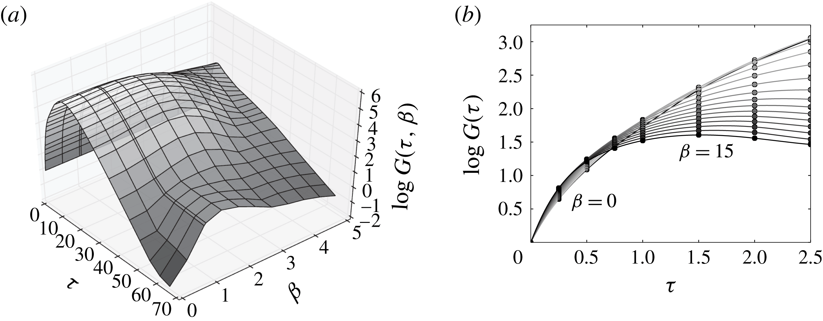
Dependence on spanwise wavenumber of the three-dimensinal transient energy growth after primary instability. (a) Surface plot of energy growth envelopes, $G(\unicode[STIX]{x1D70F},\unicode[STIX]{x1D6FD})$ , as a function of spanwise wavenumber $\unicode[STIX]{x1D6FD}$ and time $\unicode[STIX]{x1D70F}$ at $Re=540$ . (b) Enlargement of (a) for short times with $\unicode[STIX]{x1D6FD}$ from 0 to 15 in steps of 1.

Figure 12 summarizes the $\unicode[STIX]{x1D6FD}$ -dependence of the three-dimensional transient energy growth for the asymmetric flow. Optimal energy growth, $G(\unicode[STIX]{x1D70F},\unicode[STIX]{x1D6FD})$ , is plotted against spanwise wavenumber $\unicode[STIX]{x1D6FD}$ and time $\unicode[STIX]{x1D70F}$ in figure 12(a). The spanwise wavenumber of the most amplified perturbation is $\unicode[STIX]{x1D6FD}=1.052$ . Then, the global maximum energy growth is $G_{\unicode[STIX]{x1D6FD}}^{max}(540)=2.41\times 10^{5}$ at $\unicode[STIX]{x1D70F}_{\unicode[STIX]{x1D6FD}}^{max}=13.68$ . As expected, the optimal transient curves for each $\unicode[STIX]{x1D6FD}$ reach their maxima growth and after that they decrease monotonically without presenting any other local maximum; however, the asymmetric flow has a notable change in the maximum growth and time of maximum growth for $\unicode[STIX]{x1D6FD}>2.5$ . Figure 12(b) shows a close-up of figure 12(a) for short times with $\unicode[STIX]{x1D6FD}$ from 0 to 15 in steps of 1. At first glance, it is evident that the optimal growths for the higher spanwise wavenumbers are favoured at short times, nevertheless they rapidly decrease and the smaller spanwise wavenumbers become dominant. Blackburn et al. (Reference Blackburn, Sherwin and Barkley2008b ) and Cantwell et al. (Reference Cantwell, Barkley and Blackburn2010) reported analogous behaviour for steady flow in a axisymmetric pipes, and Abdessemed et al. (Reference Abdessemed, Sharma, Sherwin and Theofilis2009) also observed this behaviour for external flow.

Figure 13.

Plots of three-dimensional optimal perturbation before secondary instability, computed at $Re=540$ for $\unicode[STIX]{x1D6FD}=1.052$ . Streamwise velocity iso-surfaces of the optimal initial perturbation for $\unicode[STIX]{x1D70F}=14$ : (a) side view, (b) top view. Vorticity iso-surfaces of the optimal perturbation growth outcome at $\unicode[STIX]{x1D70F}=14$ : (c) side view, (d) top view.

In order to explore the convective mechanisms for the asymmetric flow, an optimal initial perturbation and its respective optimal growth outcome for the most amplified case with $\unicode[STIX]{x1D6FD}=1.052$ at $Re=540$ are plotted in figure 13. Streamwise velocity iso-surfaces of the optimal initial perturbation for $\unicode[STIX]{x1D70F}=14$ are shown in figure 13(a,b). It can be seen that the optimal initial condition also lies around the throat, being stronger at the shear layers and upstream from the throat with a chevron-shaped pattern, as occurred before the transition, but spreading more widely upstream and downstream from the throat. As expected, both shear layers play a major role in triggering the optimal growth. In addition, the optimal perturbation is asymmetric with respect to the channel centreline because of the upward deflection of the shear layers in the asymmetric base flow. Figure 13(c,d) illustrates vorticity iso-surfaces of the optimal perturbation growth outcome at $\unicode[STIX]{x1D70F}=14$ corresponding to the initial condition shown in figure 13(a,b). The evolution of the initial condition also becomes a wave packet and the optimal growth occurs after the recirculating regions, but this wave packet is longer in the streamwise direction compared to before the transition.

6.5 Nonlinear effects triggered by optimal perturbations

We have shown that the asymmetric flow has a subcritical bifurcation and the non-normal stability analysis demonstrated that three-dimensional optimal initial perturbations can achieve energy growth of the order of $10^{5}$ for Reynolds numbers close to the critical. In this section, we are interested in knowing the behaviour of those initial conditions in a nonlinear study, taking the relative energy level between the base flow and the optimal initial perturbation into account and, more importantly, if it is possible to raise the energy of a finite perturbation up to the top hysteretic curve by non-normal growth and nonlinear saturation.

The two-dimensional asymmetric base flow was seeded with three-dimensional optimal initial perturbations at $Re=558$ for $\unicode[STIX]{x1D6FD}_{c}=1.47$ (critical spanwise wavenumber) with four different energy levels. From the non-normal stability analysis, the time horizon was chosen to be $\unicode[STIX]{x1D70F}=15$ , so that the optimal growth in this condition is $G(15,1.47)=3.57\times 10^{5}$ . The three-dimensional DNS were performed with 8 Fourier modes. The number of modes was selected after a convergence study, documented in Isler (Reference Isler2018).

Figure 14.

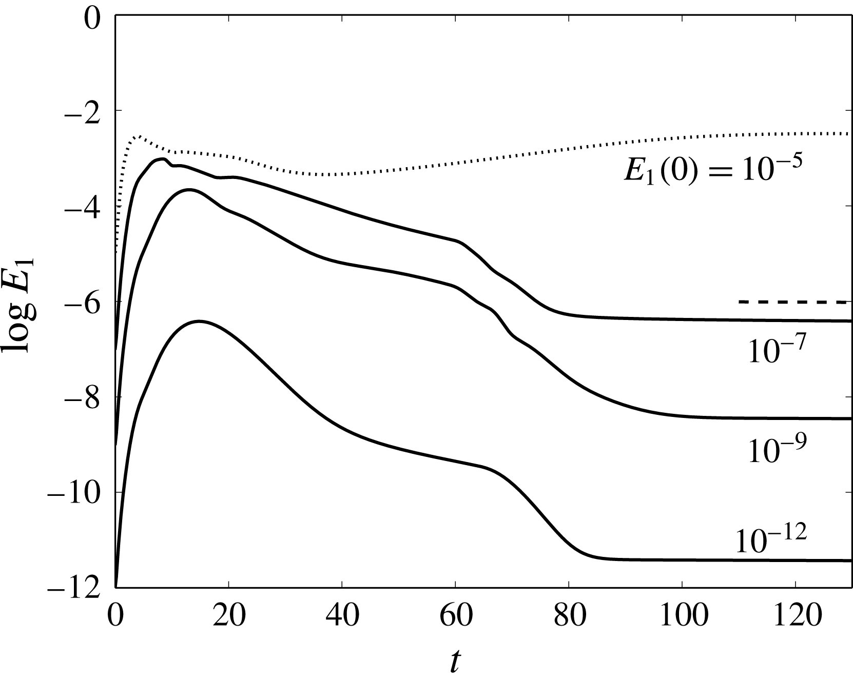
Three-dimensional DNS at $Re=558$ and $\unicode[STIX]{x1D6FD}=1.47$ seeded with optimal initial perturbations for $\unicode[STIX]{x1D70F}=15$ , using 8 Fourier modes. Nonlinear effect on energy growth for the first mode number. The dashed line represents the exponential decrease associated with the leading eigenmode.

6.5.1 Subcritical nonlinear saturation

Figure 14 shows results from three-dimensional DNS at $Re=558$ and $\unicode[STIX]{x1D6FD}=1.47$ seeded with optimal initial perturbations for $\unicode[STIX]{x1D70F}=15$ . The evolution of the energy was analysed for four different energy levels for the first Fourier mode. It can be verified that the most amplified initial condition occurred when the relative amount of energy between the base flow and the initial condition was $10^{-12}$ . Furthermore, at this relative energy level, the maximum energy growth found was $3.72\times 10^{5}$ at $t=14.84$ , which is close to the optimal growth calculated with non-normal analysis. It should also be noted that the initial conditions with the lower relative energy levels match the exponential decrease associated with the leading eigenvalue of the normal analysis after long times.

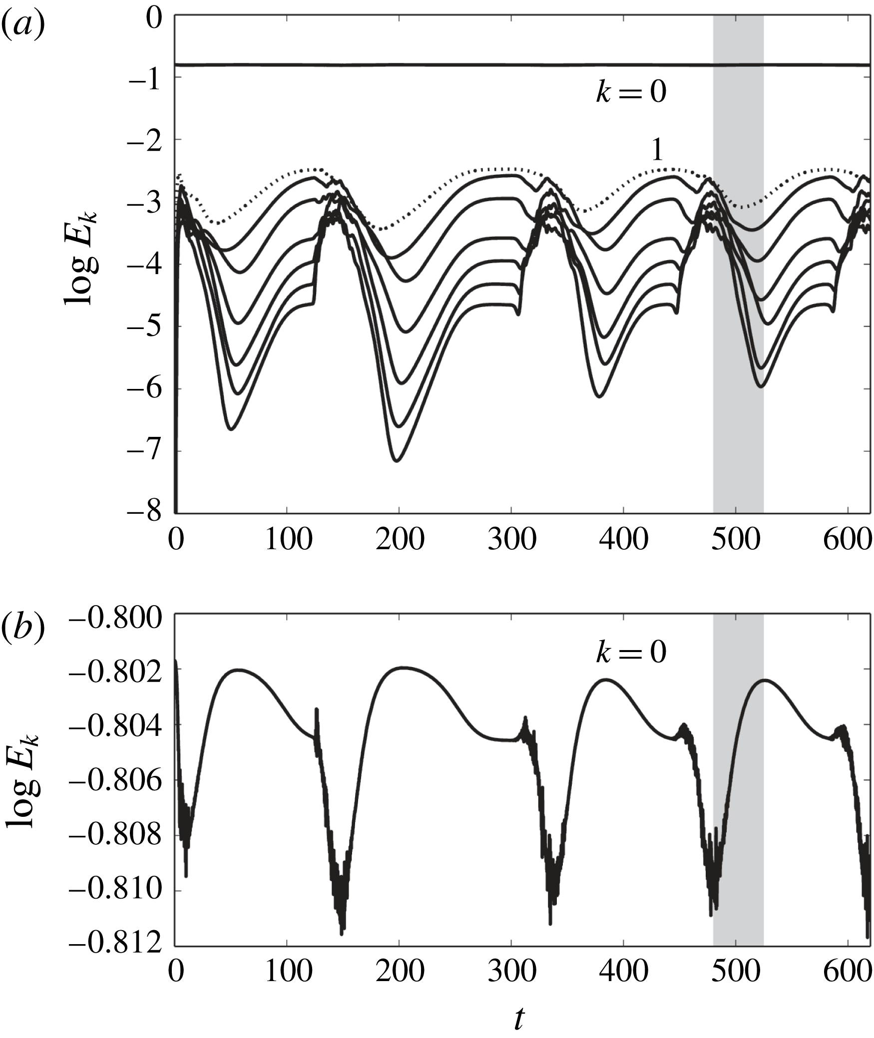
However, the initial condition with $10^{-5}$ of relative energy level did not decay monotonically after the peak growth, achieving nonlinear saturation. This is an example of a subcritical nonlinear saturation, once it was found that this flow is linearly stable at $Re=558$ . Note that the curve which saturates was marked with a different line style, and it was also highlighted in figure 15 to make it clearer. It can be seen that, in the graph at the top of figure 15, when the energies got close to the transition, the three-dimensional modes were pushed up and afterwards started to decay again. This pattern repeated with time, such that the system presented oscillatory behaviour.

Figure 15.

Time series of energies $E_{k}$ in spanwise Fourier modes of the optimal initial perturbation with relative energy level of $10^{-5}$ at $Re=558$ and $\unicode[STIX]{x1D6FD}=1.47$ .

Analysing this mechanism further, the energy of the two-dimensional base flow was subtracted from the two-dimensional Fourier mode ( $k=0$ ). Looking at the two-dimensional mode more closely, in the graph at the bottom of figure 15, it is possible to see that when the energy of the two-dimensional mode achieved a local minimum, the energies of the three-dimensional modes were going to the saturated state, so that they took energy out from the two-dimensional mode. However, the system did not stay in the saturated state and afterwards the three-dimensional modes started to give the energy back to the two-dimensional mode until it re-establishes its energy, reaching a local maximum at the end of the process. This oscillatory behaviour goes on indefinitely. Hence, we can conclude that the physical mechanism behind this remarkable behaviour occurs by energy exchange between the two- and three-dimensional modes.

This oscillatory behaviour is similar to bursts observed in channel Couette and Poiseuille flows (Waleffe Reference Waleffe1997; Zammert & Eckhardt Reference Zammert and Eckhardt2014; Brethouwer Reference Brethouwer2016). The physical mechanism of these bursts occurs by energy exchange between the mean flow ( $k=0$ ) and the smaller scales, so it agrees with our results, once the physical mechanism of energy exchange is analogous.

6.5.2 Mode interaction

Now we are going to explore the physical mechanism behind this oscillatory behaviour by flow visualization. The shaded region in figure 15 highlights the time interval in which there is an energy exchange between the two- and three-dimensional modes. The present analysis is focused on this particular region, in order to understand what is happening in the flow field.

Figure 16.

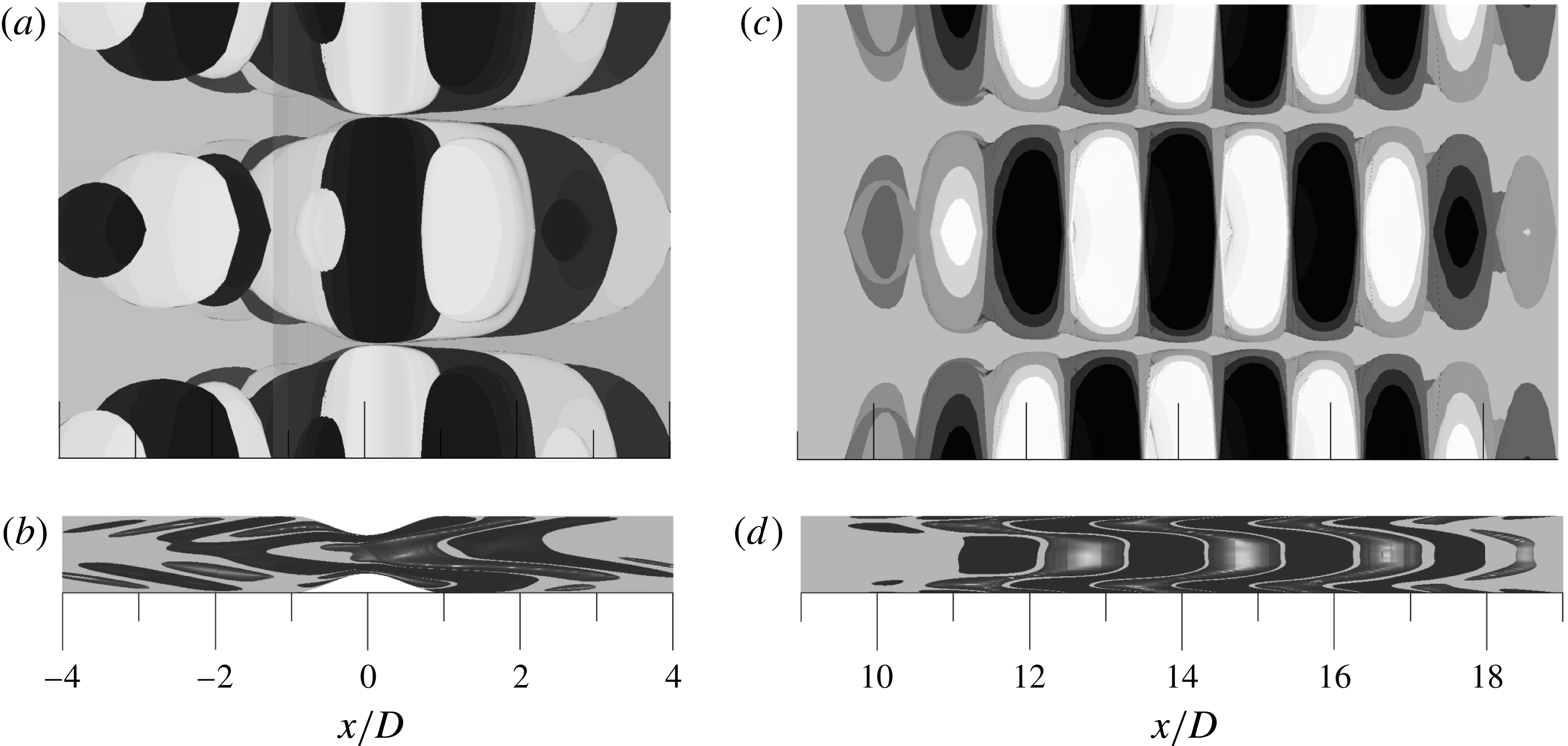
Three-dimensional DNS at $Re=558$ and $\unicode[STIX]{x1D6FD}=1.47$ . (a,c) Vorticity contours of the Fourier mode 0 (two-dimensional) subtracted from the two-dimensional base flow. (b,d) Vorticity contours of a slice from the constricted channel centreline. Contours vary from $\unicode[STIX]{x1D714}_{z}D/\bar{u}_{m}=-3.5$ (dark contours) to $\unicode[STIX]{x1D714}_{z}D/\bar{u}_{m}=3.5$ (light contours) for (a,b) and from $\unicode[STIX]{x1D714}_{z}D/\bar{u}_{m}=-0.5$ (dark contours) to $\unicode[STIX]{x1D714}_{z}D/\bar{u}_{m}=0.5$ (light contours) for (c,d).

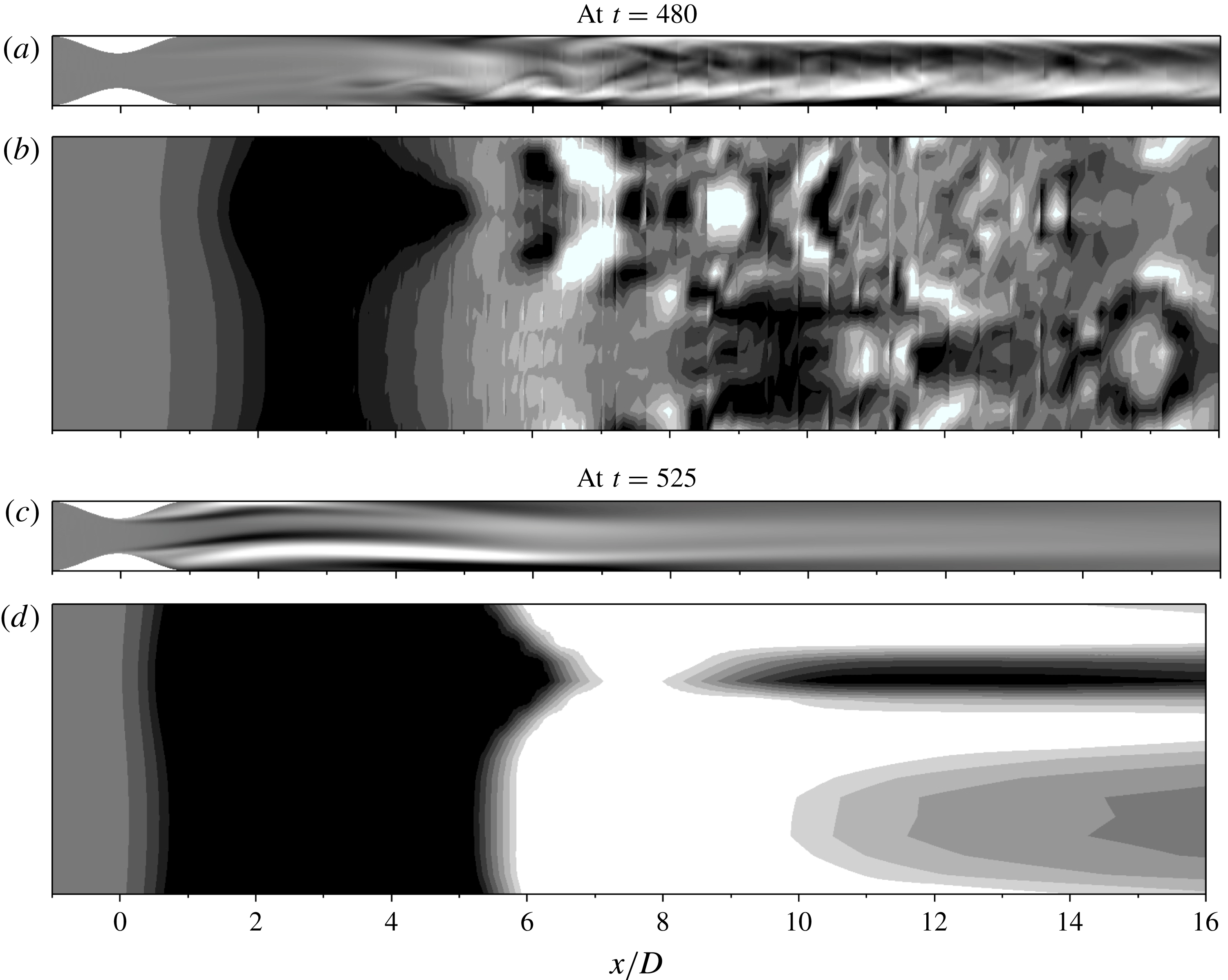
Figure 16 shows results from three-dimensional DNS at $Re=558$ and $\unicode[STIX]{x1D6FD}=1.47$ , using 8 Fourier modes. Vorticity contours of the Fourier mode 0 (two-dimensional) subtracted from the two-dimensional base flow is illustrated in figure 16(a,c). It can be seen that, at $t=480$ (local minimum energy of the two-dimensional mode), there is an intense vorticity fluctuation after the recirculating regions, demonstrating that the two-dimensional mode is strongly affected by the three-dimensional modes. On the other hand, when the two-dimensional mode achieves its local maximum at $t=525$ , all the three-dimensional disturbed flow went away downstream from the throat and afterwards the flow becomes well-behaved with a weak vorticity in the shear layers. Inspecting the three-dimensional flow in figure 16(b,d), as expected, at $t=480$ the flow is highly three-dimensional when it reaches the saturated state, so that there is a great interaction between the three-dimensional modes, not only with the two-dimensional mode as previously mentioned from figure 15. At the end of the process at $t=525$ , the three-dimensionalities almost disappear.

7 Conclusion

Results have been presented from two- and three-dimensional nonlinear simulations, and normal and non-normal stability analyses of the flow in a straight channel with a smooth constriction with 50 % occlusion. Primary and secondary global instabilities were studied in depth, so that their critical values were determined and their bifurcations were characterized by nonlinear simulations. Symmetric and asymmetric steady flows before the primary and secondary global instabilities, respectively, were also explored with respect to the transient growth behaviour, using Reynolds number as a parameter in both flows and spanwise wavenumber for the asymmetric flow. In addition, we investigated an example of subcritical nonlinear saturation with the nonlinear effects being triggered by an optimal initial perturbation in a linearly stable region, and could observe the existence of an initial energy threshold for this transition to occur. The transition process was based on the energy exchange between the two- and three-dimensional modes. All in all, the main idea behind this paper was to investigate the instability mechanisms of two consecutive bifurcations from different points of view, thus creating a complete picture of the transitions in the constricted channel.

The primary bifurcation revealed an intricate character, in which the three-dimensional Fourier modes transfer their energy to the two-dimensional mode, such that there is a symmetry breaking of the flow before the transition, creating a hysteretic region. It is noteworthy that the symmetry breaking did not happen for two-dimensional simulations, it being a three-dimensional effect. Therefore, the bifurcation is due to a three-dimensional perturbation, which transfers its energy to the two-dimensional mode, leading it to nonlinear saturation and as a consequence the symmetry breaking occurs. However, certain points still need to be clarified, and we leave them as suggestions for future work. First, the physical mechanism by which the three-dimensional modes transfer their energy to the two-dimensional mode is not completely explained. In addition, it should be verified if this transference of energy results from weakly nonlinear effects. Third, the mechanism which stabilizes the original unstable three-dimensional modes when the two-dimensional mode grows was not investigated. Finally, it can be investigated if a finite spanwise extent with end walls, as would be done in a real experiment would exhibit behaviour similar to that observed here.

The secondary instability presented subcritical behaviour of a pitchfork bifurcation and a huge hysteretic region was found, which extends far away from the critical point. Unlike what happens in the constricted channel, Rani & Sheu (Reference Rani and Sheu2006) reported that a supercritical Hopf bifurcation was obtained for the primary instability in a backward-facing step, which was firstly observed by Barkley et al. (Reference Barkley, Gomes and Henderson2002). So, although both flows are confined by parallel walls and asymmetric, they bifurcate by different paths. Hence, we can conclude that the bifurcation is notably influenced by the shear layers, since the separated flow of the backward-facing step and the constricted channel are very different.

Comparing the dependence on Reynolds number before and after the primary bifurcation, the two-dimensional maximum growth increased exponentially with $Re^{5/4}$ and $Re$ , respectively. It indicates that the flow regime changes the physical mechanism which takes the optimal initial perturbations to their maxima. In addition, after the first bifurcation, when the asymmetric flow takes place, the two-dimensional maximum growth increases with a rate given by $\unicode[STIX]{x2202}\log G_{0}^{max}/\unicode[STIX]{x2202}Re=0.0113$ , being practically the same found by Blackburn et al. (Reference Blackburn, Barkley and Sherwin2008a ) in the flow past a backward-facing step. On the other hand, the time of maximum growth increased with a different linear rate. Therefore, we believe that, although the geometries are different, the flow regime (asymmetric flow) and the channel geometry (common to both) play key roles in the sense of how the perturbation exchanges energy with the base flow. However, the location of the growing initial perturbations and their shapes will establish how far the disturbances will be convected as well as how long they will exchange energy with the base flow. As a consequence of the strong correlation between maximum growth and time of maximum growth with the Reynolds number, for the symmetric and asymmetric flows, the maximum growth increased exponentially with time of maximum growth. From this correlation we conclude that in each flow regime the initial perturbations travel to their maxima with the same constant growth rate with Reynolds number as a parameter.

A significant finding of this study was that it was possible to transition the flow to the top part of the hysteretic curve of the subcritical bifurcation (linearly stable region) by nonlinear saturation, seeding the base flow with an optimal initial perturbation with an initial energy above a certain threshold. The transition process occurred by nonlinear interaction between the two- and three-dimensional modes in oscillatory behaviour between a saturated state and a stage of redistribution of energy which brings the energy of the three-dimensional modes down again. Thus, the two-dimensional mode is crucial for the transition processes of the primary and secondary global instabilities, because in both flow regimes the two-dimensional mode led them to the nonlinear saturated state. Therefore, the energy exchange between the two- and three-dimensional modes plays a very important role in this geometry.

As a final thought throughout this context, we identified that the asymmetric flow in the constricted channel and in the backward-facing step bifurcate by different physical mechanisms, but it is intriguing that the two-dimensional maximum energy growth increases exponentially with Reynolds number by the same growth rate in both flows. Thus, it is more evidence that the asymmetric channel flow establishes how the flow exchanges energy with the perturbation, showing the importance of the geometry, even though the shear layers have different shapes. Nevertheless, the shear layers were decisive for the flow transition, with each flow exhibiting different characteristics when they bifurcate.

Acknowledgements

J.A.I. thankfully acknowledges CAPES for financial support during his PhD. J.A.I. and B.S.C. gratefully acknowledge the support from FAPESP Project (2012/50283-6).

Appendix A. Normal and non-normal stability analysis

We considered two-dimensional base flows $\boldsymbol{U}(x,y,t)$ and investigated their stability with respect to an infinitesimal three-dimensional perturbations $\boldsymbol{u}^{\prime }(x,y,z,t)$ . The evolution of the infinitesimal perturbation in a spatial domain $\unicode[STIX]{x1D6FA}$ is governed by the linearized Navier–Stokes equations:

(A 1)

$$\begin{eqnarray}\unicode[STIX]{x2202}_{t}\boldsymbol{u}^{\prime }=-(\boldsymbol{U}\boldsymbol{\cdot }\unicode[STIX]{x1D735})\boldsymbol{u}^{\prime }-(\boldsymbol{u}^{\prime }\boldsymbol{\cdot }\unicode[STIX]{x1D735})\boldsymbol{U}-\unicode[STIX]{x1D735}p^{\prime }+Re^{-1}\unicode[STIX]{x1D6FB}^{2}\boldsymbol{u}^{\prime },\quad \text{with }\unicode[STIX]{x1D735}\boldsymbol{\cdot }\boldsymbol{u}^{\prime }=0\text{ in }\unicode[STIX]{x1D6FA},\end{eqnarray}$$

where $p^{\prime }(x,y,z,t)$ is the pressure perturbation.

If we consider a system that is homogeneous in the spanwise direction $z$ , the perturbed velocity field can be decomposed into non-interacting modes, considering a Fourier modal expansion in $z$ ,

(A 2)

$$\begin{eqnarray}\boldsymbol{u}^{\prime }(x,y,z,t)=\hat{\boldsymbol{u}}(x,y,t)\text{e}^{\text{i}\unicode[STIX]{x1D6FD}z}+\text{c.c.},\end{eqnarray}$$

and similarly for $p^{\prime }$ , where the spanwise wavenumber is $\unicode[STIX]{x1D6FD}=2\unicode[STIX]{x03C0}/L_{z}$ ( $L_{z}$ is the spanwise wavelength of the instability).

In addition, the linearized equations can be defined as an operator ${\mathcal{A}}(\unicode[STIX]{x1D70F})$ to describe the action of (A 1) on an initial perturbation $\boldsymbol{u}^{\prime }(t=0)$ over a time interval $\unicode[STIX]{x1D70F}$ such that $\boldsymbol{u}^{\prime }(\unicode[STIX]{x1D70F})={\mathcal{A}}(\unicode[STIX]{x1D70F})\boldsymbol{u}^{\prime }(0)$ .

A.1 Linear stability analysis

To determine the asymptotic stability of the base flow $\boldsymbol{U}$ , we need to solve the eigensystem of this forward evolution operator ${\mathcal{A}}(\unicode[STIX]{x1D70F})$ . Since $\boldsymbol{U}$ is steady, we can use any fixed arbitrary time $T$ , as long as we obey the Nyquist criterion. The solution of the linear system (A 1) can be decomposed as a sum of eigenmodes $\boldsymbol{u}^{\prime }(\boldsymbol{x},t)=\sum _{j}\text{exp}(\unicode[STIX]{x1D70E}_{j}t)\tilde{\boldsymbol{u}}_{j}+\text{c.c.}$ , where $\unicode[STIX]{x1D70E}_{j}$ is the complex growth rate of the eigenfunction $\tilde{\boldsymbol{u}}_{j}$ . The stability is governed by the leading eigenmodes of the eigenproblem

(A 3a,b )

$$\begin{eqnarray}{\mathcal{A}}(\unicode[STIX]{x1D70F})\tilde{\boldsymbol{u}}_{j}=\unicode[STIX]{x1D707}_{j}\tilde{\boldsymbol{u}}_{j},\quad \unicode[STIX]{x1D707}_{j}\equiv \text{exp}(\unicode[STIX]{x1D70E}_{j}\unicode[STIX]{x1D70F}),\end{eqnarray}$$

where $\unicode[STIX]{x1D707}_{j}$ is called a Floquet multiplier of the forward operator ${\mathcal{A}}(\unicode[STIX]{x1D70F})$ and $\unicode[STIX]{x1D70E}_{j}$ the eigenvalues of the largest real part of the system (A 1). A mode is linearly unstable if the real part of the growth rate, $\unicode[STIX]{x1D70E}_{j}$ , is positive, which corresponds to $|\unicode[STIX]{x1D707}_{j}|>1$ . On the other hand, a mode is linearly stable when the real part of $\unicode[STIX]{x1D70E}_{j}$ is negative, which corresponds to $|\unicode[STIX]{x1D707}_{j}|<1$ . For normal stability analysis, the velocity boundary conditions that were imposed on this system are $\boldsymbol{u}^{\prime }=\mathbf{0}$ on boundaries where Dirichlet conditions are specified for the base flow, and $\unicode[STIX]{x2202}\boldsymbol{u}^{\prime }/\unicode[STIX]{x2202}\boldsymbol{n}=\mathbf{0}$ on boundaries where Neumann conditions are specified for the base flow. Further details on the algorithms for the stability calculations are given in Carmo et al. (Reference Carmo, Sherwin, Bearman and Willden2008).

A.2 Optimal transient growth

Transient growth analysis can predict the largest possible growth in energy for a specific system governed by a linear differential equation. Thus, the idea behind this method is to search for an initial condition, $\boldsymbol{u}^{\prime }(0)$ , which will give us the largest growth. The formalism is as follows. The transient growth is defined with respect to the energy norm of the perturbation. If the norm of the initial perturbation is $\Vert \boldsymbol{u}^{\prime }(0)\Vert =\langle \boldsymbol{u}^{\prime }(0),\boldsymbol{u}^{\prime }(0)\rangle =1$ , where $\langle \cdot ,\cdot \rangle$ denotes the standard $L_{2}$ inner product, then the energy of the perturbation after time $\unicode[STIX]{x1D70F}$ , normalized with the initial energy, is

(A 4)

$$\begin{eqnarray}\frac{E(\unicode[STIX]{x1D70F})}{E(0)}=\langle \boldsymbol{u}^{\prime }(\unicode[STIX]{x1D70F}),\boldsymbol{u}^{\prime }(\unicode[STIX]{x1D70F})\rangle =\langle {\mathcal{A}}(\unicode[STIX]{x1D70F})\boldsymbol{u}^{\prime }(0),{\mathcal{A}}(\unicode[STIX]{x1D70F})\boldsymbol{u}^{\prime }(0)\rangle =\langle \boldsymbol{u}^{\prime }(0),{\mathcal{A}}^{\ast }(\unicode[STIX]{x1D70F}){\mathcal{A}}(\unicode[STIX]{x1D70F})\boldsymbol{u}^{\prime }(0)\rangle ,\end{eqnarray}$$

where $E$ is the kinetic energy per unit mass of a perturbation and the operator ${\mathcal{A}}^{\ast }$ is the adjoint of the forward operator ${\mathcal{A}}$ . The action of ${\mathcal{A}}^{\ast }$ is obtained by integrating the adjoint linearized Navier–Stokes equations

(A 5)

$$\begin{eqnarray}\unicode[STIX]{x2202}_{t}\boldsymbol{u}^{\ast }=-(\boldsymbol{U}\boldsymbol{\cdot }\unicode[STIX]{x1D735})\boldsymbol{u}^{\ast }-(\unicode[STIX]{x1D735}\boldsymbol{U})^{\text{T}}\boldsymbol{\cdot }\boldsymbol{u}^{\ast }-\unicode[STIX]{x1D735}p^{\ast }+Re^{-1}\unicode[STIX]{x1D6FB}^{2}\boldsymbol{u}^{\ast },\quad \text{with }\unicode[STIX]{x1D735}\boldsymbol{\cdot }\boldsymbol{u}^{\ast }=0\text{ in }\unicode[STIX]{x1D6FA},\end{eqnarray}$$

backwards over the time interval $\unicode[STIX]{x1D70F}$ . Thus, to compute the optimal growth of the perturbation, we need to act the symmetric operator ${\mathcal{A}}^{\ast }(\unicode[STIX]{x1D70F}){\mathcal{A}}(\unicode[STIX]{x1D70F})$ on $\boldsymbol{u}^{\prime }$ . Therefore, the optimal growth is obtained from the leading eigenmodes of

(A 6)

$$\begin{eqnarray}{\mathcal{A}}^{\ast }(\unicode[STIX]{x1D70F}){\mathcal{A}}(\unicode[STIX]{x1D70F})\boldsymbol{v}_{j}=\unicode[STIX]{x1D706}_{j}\boldsymbol{v}_{j},\end{eqnarray}$$

where $\unicode[STIX]{x1D706}_{j}$ and $\boldsymbol{v}_{j}$ are the eigenvalues and eigenmodes of ${\mathcal{A}}^{\ast }(\unicode[STIX]{x1D70F}){\mathcal{A}}(\unicode[STIX]{x1D70F})$ , respectively, with $\Vert \boldsymbol{v}\Vert =1$ . The eigenvalues are non-negative and we assume ordering $\unicode[STIX]{x1D706}_{1}\geqslant \unicode[STIX]{x1D706}_{2}\geqslant \cdots \,$ . Thus, the optimal energy growth, $G(\unicode[STIX]{x1D70F})$ , obtained at time $\unicode[STIX]{x1D70F}$ is

(A 7)

$$\begin{eqnarray}G(\unicode[STIX]{x1D70F})=\max _{\Vert \boldsymbol{u}^{\prime }(0)\Vert =1}\frac{E(\unicode[STIX]{x1D70F})}{E(0)}=\max _{j}\unicode[STIX]{x1D706}_{j}=\unicode[STIX]{x1D706}_{1}.\end{eqnarray}$$

The boundary conditions for computing the eigenvalues of ${\mathcal{A}}^{\ast }(\unicode[STIX]{x1D70F}){\mathcal{A}}(\unicode[STIX]{x1D70F})$ were homogeneous Dirichlet, i.e. $\boldsymbol{u}^{\prime }=\mathbf{0}$ , on boundaries where Dirichlet and Neumann conditions are specified for the base flow, for both the operator ${\mathcal{A}}(\unicode[STIX]{x1D70F})$ and ${\mathcal{A}}^{\ast }(\unicode[STIX]{x1D70F})$ . Although, this kind of boundary condition is not rigorously correct for the outflow boundary, we have extended the channel long enough to ensure that the influence of that was negligible. Further details on the transient growth analysis can be seen in Blackburn et al. (Reference Blackburn, Barkley and Sherwin2008a ) and Cantwell et al. (Reference Cantwell, Barkley and Blackburn2010).

In order to investigate the $Re$ - and $\unicode[STIX]{x1D6FD}$ -dependence on the maximum energy growth for two- and three-dimensional flows, two important quantities are defined as follows:

(A 8)

$$\begin{eqnarray}G_{\unicode[STIX]{x1D6FD}}^{max}(Re)=\max _{\unicode[STIX]{x1D70F}}G(\unicode[STIX]{x1D70F},Re,\unicode[STIX]{x1D6FD})\end{eqnarray}$$

and

(A 9)

$$\begin{eqnarray}\unicode[STIX]{x1D70F}_{\unicode[STIX]{x1D6FD}}^{max}(Re)=\arg \max _{\unicode[STIX]{x1D70F}}G(\unicode[STIX]{x1D70F},Re,\unicode[STIX]{x1D6FD}).\end{eqnarray}$$

$G_{\unicode[STIX]{x1D6FD}}^{max}$ is the maximum possible energy growth at a given Reynolds number and spanwise wavenumber over all time horizons and $\unicode[STIX]{x1D70F}_{\unicode[STIX]{x1D6FD}}^{max}$ is the time in which it occurs.

A more detailed description of the time-stepper approach used here may be found in Tuckerman & Barkley (Reference Tuckerman, Barkley, Doedel and Tuckerman2000) and Barkley, Blackburn & Sherwin (Reference Barkley, Blackburn and Sherwin2008).

References

Abdessemed, N., Sharma, A. S., Sherwin, S. J. & Theofilis, V. 2009 Transient growth analysis of the flow past a circular cylinder. Phys. Fluids 21, 044103.Google Scholar

Barkley, D., Blackburn, H. M. & Sherwin, S. J. 2008 Direct optimal growth analysis for timesteppers. Intl J. Numer. Meth. Fluids 57, 1435–1458.Google Scholar

Barkley, D., Gomes, G. M. & Henderson, R. D. 2002 Three-dimensional instability in flow over a backward-facing step. J. Fluid Mech. 473, 167–190.Google Scholar

Blackburn, H. M., Barkley, D. & Sherwin, S. J. 2008a Convective instability and transient growth in flow over a backward-facing step. J. Fluid Mech. 603, 271–304.Google Scholar

Blackburn, H. M., Sherwin, S. J. & Barkley, D. 2008b Convective instability and transient growth in steady and pulsatile stenotic flows. J. Fluid Mech. 607, 267–277.Google Scholar

Brethouwer, G. 2016 Linear instabilities and recurring bursts of turbulence in rotating channel flow simulations. Phys. Rev. Fluids 1, 054404.Google Scholar

Cantwell, C. D. & Barkley, D. 2010 Computational study of subcritical response in flow past a circular cylinder. Phys. Rev. E 82, 026315.Google Scholar

Cantwell, C. D., Barkley, D. & Blackburn, H. M. 2010 Transient growth analysis of flow through a sudden expansion in a circular pipe. Phys. Fluids 22, 034101.Google Scholar

Carmo, B. S., Sherwin, S. J., Bearman, P. W. & Willden, R. H. J. 2008 Wake transition in the flow around two circular cylinders in staggered arrangements. J. Fluid Mech. 597, 1–29.Google Scholar

Chun, K. B. & Sung, H. J. 1996 Control of turbulent separated flow over a backward-facing step by local forcing. Exp. Fluids 21, 417–426.Google Scholar

Farrell, B. F. 1988 Optimal excitation of perturbations in viscous shear flow. J. Fluid Mech. 31 (8), 2093–2102.Google Scholar

Griffith, M. D., Leweke, T., Hourigan, K. & Anderson, W. P. 2007 Wake behaviour and instability of flow through a partially blocked channel. J. Fluid Mech. 582, 319–340.Google Scholar

Griffith, M. D., Leweke, T., Thompson, M. C. & Hourigan, K. 2008 Steady inlet flow in stenotic geometries: convective and absolute instabilities. J. Fluid Mech. 616, 111–133.Google Scholar

Griffith, M. D., Thompson, M. C., Leweke, T. & Hourigan, K. 2010 Convective instability in steady stenotic flow: optimal transient growth and experimental observation. J. Fluid Mech. 655, 504–514.Google Scholar

Guevel, Y., Boutyour, H. & Cadou, J. M. 2011 Automatic detection and branch switching methods for steady bifurcation in fluid mechanics. J. Comput. Phys. 230 (9), 3614–3629.Google Scholar

Isler, J. A.2018 Computational study in fluid mechanics of bio-inspired geometries: constricted channel and paediatric ventricular assist device. PhD thesis, University of São Paulo.Google Scholar

Karniadakis, G. E. 1990 Spectral element–Fourier methods for incompressible turbulent flows. Comput. Meth. Appl. Mech. Engng 80, 367–380.Google Scholar

Karniadakis, G. E., Israeli, M. & Orszag, S. A. 1991 High-order splitting methods for the incompressible Navier–Stokes equations. J. Comput. Phys. 97, 414–443.Google Scholar

Karniadakis, G. E. & Sherwin, S. J. 2005 Spectral/hp Element Methods for Computational Fluid Dynamics, 2nd edn. Oxford University Press.Google Scholar

Mao, X., Sherwin, S. J. & Blackburn, H. M. 2009 Transient growth and bypass transition in stenotic flow with a physiological waveform. Theor. Comput. Fluid Dyn. 25, 31–42.Google Scholar

Pitt, R.2005 Numerical simulation of fluid mechanical phenomena in idealised physiological geometries: stenosis and double bend. PhD thesis, Imperial College London.Google Scholar

Pitt, R. E., Sherwin, S. J. & Theofilis, V. 2004 Biglobal stability analysis of steady flow in constricted channel geometries. Intl J. Numer. Meth. Fluids 47, 1229–1235.Google Scholar

Rani, H. P. & Sheu, W. H. 2006 Nonlinear dynamics in a backward-facing step flow. Phys. Fluids 18, 084101.Google Scholar

Reddy, S. C. & Henningson, D. S. 1993 Energy growth in viscous channel flows. J. Fluid Mech. 252, 209–238.Google Scholar

Samuelsson, J., Tammisola, O. & Juniper, M. P. 2015 Breaking axi-symmetry in stenotic flow lowers the critical transition Reynolds number. Phys. Fluids 27, 104103.Google Scholar

Schmid, P. J. & Henningson, D. S. 1994 Optimal energy density growth in Hagen–Poiseuille flow. J. Fluid Mech. 277, 197–225.Google Scholar

Sheard, G. J. & Blackburn, H. M. 2010 Steady inflow through a model aneurysm: global and transient stability. In 17th Australasian Fluid Mechanics Conference, Auckland, New Zealand. Australasian Fluid Mechanics Society.Google Scholar

Sherwin, S. J. & Blackburn, H. M. 2005 Three-dimensional instabilities and transition of steady and pulsatile axisymmetric stenotic flows. J. Fluid Mech. 533, 297–327.Google Scholar

Smith, D. M. & Blackburn, H. M. 2010 Transient growth analysis for axisymmetric pulsatile pipe flows in a rigid straight circular pipe. In 17th Australasian Fluid Mechanics Conference, Auckland, New Zealand. Australasian Fluid Mechanics Society.Google Scholar

Tuckerman, L. S. & Barkley, D. 2000 Bifurcation analysis for timesteppers. In Numerical Methods for Bifurcation Problems and Large-Scale Dynamical Systems (ed. Doedel, E. & Tuckerman, L. S.), pp. 453–466. Springer.Google Scholar

Waleffe, F. 1997 On a self-sustaining process in shear flows. Phys. Fluids 9 (4), 883–900.Google Scholar

Zammert, S. & Eckhardt, B. 2014 Periodically bursting edge states in plane Poiseuille flow. Fluid Dyn. Res. 46, 041419.Google Scholar

Figure 1.Computational domain $\unicode[STIX]{x1D6FA}$ and geometric parameters which define the constricted channel geometry (not to scale).

Figure 2.Close-up of the computational mesh around the throat; the dimension is given in terms of channel height $D$. The mesh has 2974 spectral elements.

Table 1.Convergence of the two-dimensional optimal growth at $\unicode[STIX]{x1D70F}=16$ for $Re=720$ with respect to the variation of the spectral element polynomial order $N$, computed with $M_{1}$.

Figure 3.Two-dimensional base flow close to primary instability at $Re=270$. (a) Vorticity contours and streamlines showing the recirculating regions. (b) Velocity profiles. Reattachment occurs at $x/D=2.82$.

Table 2.Convergence of the two-dimensional optimal growth at $\unicode[STIX]{x1D70F}=16$ for $Re=720$ with respect to the variation of the inflow and outflow lengths, computed with polynomial order $N=6$.

Figure 4.Linear stability analysis for the primary instability. (a) Plot of the leading eigenvalues, $\unicode[STIX]{x1D70E}$, against spanwise wavenumber $\unicode[STIX]{x1D6FD}$ for different Reynolds numbers. Inset: the critical Reynolds number for $\unicode[STIX]{x1D6FD}=0$ is $Re=281.2$, determined by interpolation. (b) Neutral stability curve for the symmetric steady flow in the constricted channel. In the region on the right-hand side of the curve (dark region) the two-dimensional flow is linearly unstable to infinitesimal three-dimensional perturbation. The critical Reynolds number is $Re_{c}=278.8$.

Figure 5.(a) Energy diagram of the symmetric steady flow for $\unicode[STIX]{x1D6FD}=0.45$. The diagram was built with the energy of the two-dimensional component of the Fourier modes ($k=0$). (b) Velocity contours perpendicular to the $x$-direction of the three-dimensional flow at $Re=270$, when it achieves nonlinear saturation of the two-dimension Fourier mode.

Figure 6.Dependence on Reynolds number of the two-dimensional transient energy growth before primary instability. (a) Energy growth envelopes, $G(\unicode[STIX]{x1D70F})$, as a function of $\unicode[STIX]{x1D70F}$ for Reynolds number varying from 45 up to 270. The dashed line represents the exponential decrease associated with the leading eigenmode. (b) Logarithmic contours for two-dimensional optimal energy growth, $G(\unicode[STIX]{x1D70F},Re)$, as a function of $\unicode[STIX]{x1D70F}$ and $Re$. The critical Reynolds number for the first growth is $Re_{E}=49.5$. The dotted-line curve shows the local of maximum energy growth as a function of $\unicode[STIX]{x1D70F}$. Variation of maximum (c) growth and (d) time as a function of $Re^{5/4}$. Values of $\log G_{0}^{max}$ and $\unicode[STIX]{x1D70F}_{0}^{max}$ increase linearly with $Re^{5/4}$. (e) Maximum energy growth as a function of time of maximum growth for the Reynolds number range from $Re_{E}$ to $Re_{c}$. The value of $\log G_{0}^{max}$ grows linearly with $\unicode[STIX]{x1D70F}_{0}^{max}$.

Figure 7.Plots of two-dimensional logarithmic contours of energy before primary instability, computed at $Re=270$. (a) Optimal initial perturbation for $\unicode[STIX]{x1D70F}=6$. (b) Optimal perturbation growth outcome at $\unicode[STIX]{x1D70F}=6$. The vectors represent the velocity field.

Figure 8.Two-dimensional base flow close to secondary instability. Vorticity contours and streamlines, showing the recirculating regions at (a) $Re=540$ and (b) $Re=720$. (c) Velocity profiles at $Re=540$. Reattachments occur at $x/D=1.82$ and $x/D=6.04$ for$Re=540$.

Figure 9.Linear stability analysis for the secondary instability. (a) Plot of the leading eigenvalues, $\unicode[STIX]{x1D70E}$, against spanwise wavenumber $\unicode[STIX]{x1D6FD}$ for different Reynolds numbers. (b) Neutral stability curve for the asymmetric steady flow in the constricted channel. In the region on the right hand side of the curve (dark region) the two-dimensional flow is unstable to infinitesimal three-dimensional perturbation. The critical Reynolds number is $Re_{c}=562.0$.

Figure 10.Diagram of the subcritical bifurcation of the asymmetric steady flow for $\unicode[STIX]{x1D6FD}=1.47$. The solid circles represent the DNS seeded with the nonlinear saturation of the unstable base flow at $Re=720$ and the hollow circles with a linear combination of the base flow and the leading eigenmode.

Figure 11.Dependence on Reynolds number of the two-dimensional transient energy growth after primary instability. (a) Energy growth envelopes, $G(\unicode[STIX]{x1D70F})$, as a function of $\unicode[STIX]{x1D70F}$ for Reynolds number varying from 450 up to 720. (b) Logarithmic contour plot for two-dimensional optimal energy growth, $G(\unicode[STIX]{x1D70F},Re)$, as a function of $\unicode[STIX]{x1D70F}$ and $Re$. The dotted-line curve shows the local of maximum energy growth as a function of $\unicode[STIX]{x1D70F}$. Variation of maximum (c) growth and (d) time as a function of $Re$. The $\log G_{0}^{max}$ and $\unicode[STIX]{x1D70F}_{0}^{max}$ increase linearly with $Re$. (e) Maximum energy growth as a function of time of maximum growth for the Reynolds number range from $450$ to $720$. The $\log G_{0}^{max}$ grows linearly with $\unicode[STIX]{x1D70F}_{0}^{max}$.

Figure 12.Dependence on spanwise wavenumber of the three-dimensinal transient energy growth after primary instability. (a) Surface plot of energy growth envelopes, $G(\unicode[STIX]{x1D70F},\unicode[STIX]{x1D6FD})$, as a function of spanwise wavenumber $\unicode[STIX]{x1D6FD}$ and time $\unicode[STIX]{x1D70F}$ at $Re=540$. (b) Enlargement of (a) for short times with $\unicode[STIX]{x1D6FD}$ from 0 to 15 in steps of 1.

Figure 13.Plots of three-dimensional optimal perturbation before secondary instability, computed at $Re=540$ for $\unicode[STIX]{x1D6FD}=1.052$. Streamwise velocity iso-surfaces of the optimal initial perturbation for $\unicode[STIX]{x1D70F}=14$: (a) side view, (b) top view. Vorticity iso-surfaces of the optimal perturbation growth outcome at $\unicode[STIX]{x1D70F}=14$: (c) side view, (d) top view.

Figure 14.Three-dimensional DNS at $Re=558$ and $\unicode[STIX]{x1D6FD}=1.47$ seeded with optimal initial perturbations for $\unicode[STIX]{x1D70F}=15$, using 8 Fourier modes. Nonlinear effect on energy growth for the first mode number. The dashed line represents the exponential decrease associated with the leading eigenmode.

Figure 15.Time series of energies $E_{k}$ in spanwise Fourier modes of the optimal initial perturbation with relative energy level of $10^{-5}$ at $Re=558$ and $\unicode[STIX]{x1D6FD}=1.47$.

Figure 16.Three-dimensional DNS at $Re=558$ and $\unicode[STIX]{x1D6FD}=1.47$. (a,c) Vorticity contours of the Fourier mode 0 (two-dimensional) subtracted from the two-dimensional base flow. (b,d) Vorticity contours of a slice from the constricted channel centreline. Contours vary from $\unicode[STIX]{x1D714}_{z}D/\bar{u}_{m}=-3.5$ (dark contours) to $\unicode[STIX]{x1D714}_{z}D/\bar{u}_{m}=3.5$ (light contours) for (a,b) and from $\unicode[STIX]{x1D714}_{z}D/\bar{u}_{m}=-0.5$ (dark contours) to $\unicode[STIX]{x1D714}_{z}D/\bar{u}_{m}=0.5$ (light contours) for (c,d).

Article contents

Bifurcations and convective instabilities of steady flows in a constricted channel

Abstract

JFM classification

Information

1 Introduction

2 Problem definition

3 Methodology

3.1 Two-dimensional base flow calculation

3.2 Nonlinear analysis

4 Numerical approach

5 Primary global instability

5.1 Base flow characteristics

5.2 Normal stability analysis

5.3 Nonlinear characterization of the bifurcation

5.4 Non-normal stability analysis

5.4.1 Dependence on Reynolds number

6 Secondary global instability

6.1 Base flow characteristics

6.2 Normal stability analysis

6.3 Nonlinear characterization of the bifurcation

6.4 Non-normal stability analysis

6.4.1 Dependence on Reynolds number

6.4.2 Dependence on spanwise wavenumber

6.5 Nonlinear effects triggered by optimal perturbations

6.5.1 Subcritical nonlinear saturation

6.5.2 Mode interaction

7 Conclusion

Acknowledgements

Appendix A. Normal and non-normal stability analysis

A.1 Linear stability analysis

A.2 Optimal transient growth

References

Save article to Kindle

Save article to Dropbox

Save article to Google Drive

Reply to: Submit a response

Your details

You have entered the maximum number of contributors

Conflicting interests