2. Wheeled Mobile Robot Modeling

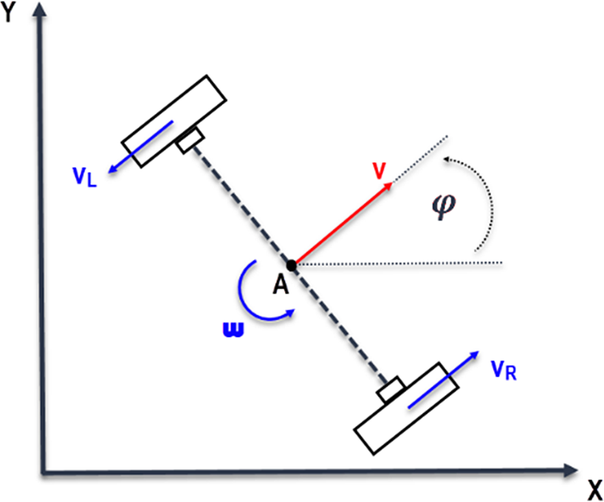
In this section kinematic and dynamic equations of a single differential drive mobile robot will be presented. Assume that the WMR has two active wheels mounted on one axis and a front passive wheel. The vehicle configuration is described by three generalized coordinates: the Cartesian coordinates $\left( {{x_c},{y_c}} \right)$ of the center of mass measured in the fixed reference frame and the angle $\;\theta $ characterizing the orientation of the platform with respect to the axis X, see Fig. 1. The configuration vector is, therefore, $\boldsymbol{q}\; = \;{\left[ {{x_c},{y_c},\theta } \right]^T}$ .

Fig. 1.

The kinematic model of a single differential drive mobile robot.

2.1 Kinematics model

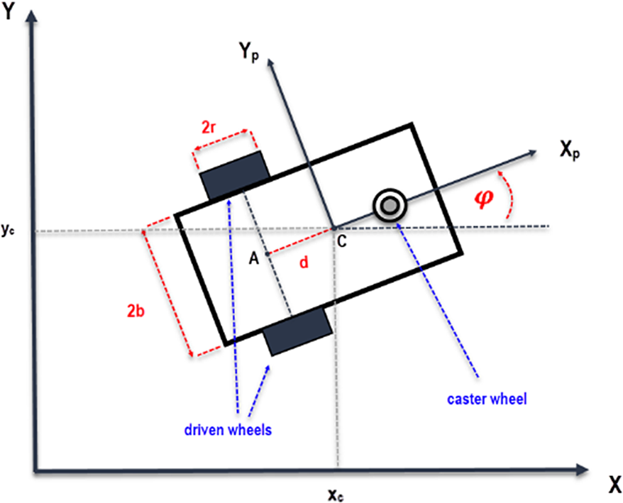
Assume that the robot can only move along the vehicle longitudinal axis and the wheels roll without slipping in the horizontal plane. By considering these assumptions, the robot will have a kinematic constraint called a nonholonomic constraint. Assume that the center of mass of the mobile robot is at some position $\left( {{x_c},{y_c}} \right)$ and orientation $\varphi $ which can be expressed as a state vector $\boldsymbol{q}(t) = {\left[ {\begin{array}{*{20}{c}}{{x_C}(t)}\quad {}{{y_C}(t)}\quad {}{\varphi (t)}\end{array}} \right]^T}$ . The pure rolling and non-slipping constraint can be expressed in the Pfaffian form as [Reference Siciliano and Khatib34]:

(1) \begin{align}{\dot x_c}\,{\textrm{sin}}\,\varphi - {\dot y_c}\,{\textrm{cos}}\,\varphi + \dot \varphi d = 0\end{align}

where ${\dot x_c}\;and\;{\dot y_c}$ are the robot velocity components in the Cartesian plane, $\dot \varphi $ is the angular velocity, and d is the distance between A (the midpoint of the segment joining the centers of the two wheels) and c (the center of mass of the robot), see Fig. 2.

Fig. 2.

Single robot specification.

The above equation can be written in the matrix form

(2) \begin{align}{\textbf{A}}({{\textbf{q}}}).\,{\dot{\textbf{q}}} = 0\end{align}

where ${{\textbf{A}}}({{\textbf{q}}}) = \left[ {sin}\varphi, {-cos}\varphi, {d} \right]$ , and ${\dot{\textbf{q}}} = {\left[ {{{\dot x}_c},{{\dot y}_c},\dot \varphi } \right]^T}$ denotes the velocities vector. Therefore, the kinematic model of the system can be written as the following

(3) \begin{align}{\dot{\textbf{q}}}(t) = {{\textbf{S}}}({{\textbf{q}}}){{\textbf{v}}}\end{align}

where ${{\textbf{v}}} = {\left[ {{{{{\dot{\unicode[Times]{x03B8}} }}}_{\textrm{r}}},{{{{\dot{\unicode[Times]{x03B8}} }}}_{\textrm{l}}}} \right]^{\textrm{T}}}{\textrm{and}}{{{\dot{\unicode[Times]{x03B8}} }}_{\textrm{r}}},{{{\dot{\unicode[Times]{x03B8}} }}_{\textrm{l}}}$ are the velocities of the right and the left wheels, respectively.

To derive the matrix ${{\textbf{S}}}({{\textbf{q}}})$ , the position of the center of mass can be written with respect to point A as follows

\begin{align*}{x_c}(t) = {x_a} + d{\textrm{cos}}\;\varphi \end{align*}

(4) \begin{align}{y_c}(t) &= {y_a} + d{\textrm{sin}\varphi} \nonumber\\[6pt] \varphi (t) &= \varphi (t)\end{align}

Differentiating Eq. 4 with respect to time yields

(5) \begin{align}\begin{array}{*{20}{c}}{{{\dot x}_c}(t) = v\textrm{cos}\varphi - d\omega \textrm{sin}\varphi }\\{{{\dot y}_c}(t) = v\textrm{sin}\varphi + d\omega \textrm{cos}\varphi }\\\, \, {\dot \varphi (t) = \omega \, \, \, \, \, \, \, \, \, \, \, \, \, \, \, \, \, \, \, \, \;\;\;\;\;}\end{array}\end{align}

where $v$ and $\omega $ are the linear and the angular velocities of the vehicle, respectively. Since the linear velocity of each wheel of the robot in the robot frame $\left( {{{\textrm{X}}_p},\;{{\textrm{Y}}_p}} \right)$ is ${v_{r,l}} = r{\dot \theta _{r,l}}$ , then the linear and the angular velocities of the vehicle in the robot frame can be obtained as

(6) \begin{align}v = {{{v_r} + {v_l}} \over 2} = r{{{{\dot \theta }_r} + {{\dot \theta }_l}} \over 2}\end{align}

(7) \begin{align}\omega = r{{{{\dot \theta }_r} - {{\dot \theta }_l}} \over {2b}}\end{align}

where r is the radius of the driving wheel, ${\dot \theta _r},\;{\dot \theta _l}$ are the angular velocities of the right and left wheels, respectively, and b is half the distance between the two wheels centers.

By substituting Eq. 6 and Eq. 7 in Eq. 5, the kinematic model of the WMR in Eq. 3 can be derived by the following

(8) \begin{align}{\dot{\textbf{q}}}(t) = \left[ \begin{array}{c@{\quad}c} \dfrac{r}{2b}\left( {b{\textrm{cos}}\varphi\,-\,d{\textrm{sin}}\varphi } \right) & {}\dfrac{r}{2b}\left( {b{\textrm{cos}}\varphi\,+\,d{\textrm{sin}}\varphi } \right) \\[9pt] \dfrac{r}{2b}\left( {b{\textrm{sin}}\varphi\,+\,d{\textrm{cos}}\varphi } \right) & {}\dfrac{r}{2b}(b{\textrm{sin}}\varphi\,-\,d{\textrm{cos}}\varphi) \\ \dfrac{r}{2b} & {}{ - \dfrac{r}{2b}}\end{array} \right]\left[ \begin{array}{c} {{{\dot \theta }_r}} \\[4pt] {{{\dot \theta }_l}} \end{array} \right]\end{align}

2.2 Dynamics model

In the following, the Lagrange formulation is used to obtain the dynamic model of the WMR system subject to the kinematic constraint in Eq. 2. The Lagrangian $\mathcal{L}$ of a mechanical system is defined as the difference between its kinetic and potential energy

(9) \begin{align}\mathcal{L}({{{\textbf{q}}},{\dot{\textbf{q}}}}) = T({{{\textbf{q}}},{\dot{\textbf{q}}}}) - U({{\textbf{q}}})\end{align}

where $T$ and $U$ are the kinetic energy and the potential energy of the system, respectively. The Lagrange equations, in this case, are

(10) \begin{align}\frac{d}{{dt}}\left( {\frac{{\partial \mathcal{L}}}{{\partial {\dot{\textbf{q}}}}}} \right) - \frac{{\partial \mathcal{L}}}{{\partial {{\textbf{q}}}}} = {{\textbf{B}}}({{\textbf{q}}}){{\boldsymbol\tau }} + {{\textbf{A}}}{({{\textbf{q}}})^T}{{\boldsymbol\lambda }}\end{align}

where ${{\textbf{B}}}({{\textbf{q}}})$ is the input transformation matrix, ${{\boldsymbol\tau }} = \left[ {{\tau _r}{\tau _l}} \right]$ represents the actuating torques of the right and left wheels, and ${{\boldsymbol\lambda }}$ is a vector of Lagrangian multipliers. The term ${{\textbf{A}}}{({{\textbf{q}}})^T}{{\boldsymbol\lambda }}$ represents the vector of reaction forces at the generalized coordinate level.

The kinetic energy of the system can be written as

(11) \begin{align}T = {1 \over 2}m\left( {\dot x_c^2 + \dot y_c^2} \right) + {1 \over 2}I{\dot \varphi ^2}\end{align}

where

\begin{align*}m = \left( {{m_p} + 2{m_w}} \right)\end{align*}

\begin{align*}\;\;I = {I_{zp}} + 2{I_{zw}} + 2{m_w}\left( {{d^2} + {b^2}} \right)\end{align*}

where m is the total mass of the robot, ${m_p}$ is the mass of the platform without the driven wheels and actuators, ${m_w}$ is the mass of the wheels and their actuators, and ${I_{zp}}\;and\;{I_{zw}}$ are the moments of inertia of the wheels and the platform, respectively.

Since the potential energy of the system is equal to zero, hence the Lagrangian function is equal to the kinetic energy that is, $\mathcal{L}\left( {q,\dot q} \right) = T\left( {q,\dot q} \right)$ .

By substituting the kinetic energy in Eq. 11 into Eq. 10, we obtain the equation of motion of the WMR

\begin{align*}m{\ddot x_c} = \left( {\frac{{{\tau _R}}}{r} + \frac{{{\tau _L}}}{r}} \right){\textrm{cos}}\varphi + {C_1}\end{align*}

\begin{align*}m{\ddot y_c} = \left( {\frac{{{\tau _R}}}{r} + \frac{{{\tau _L}}}{r}} \right){\textrm{sin}}\varphi + {C_2}\end{align*}

(12) \begin{align}I\ddot \varphi = L\left( {{{{\tau _R}} \over r} - {{{\tau _L}} \over r}} \right) + {C_3}\end{align}

where ${C_1},\;\;{C_{2,}}\;and\;{C_3}$ are coefficients related to the kinetic constraints. Eq. 12 can be written in the matrix form

(13) \begin{align}{{\textbf{M}}}({{\textbf{q}}}){\ddot{\textbf{q}}} + {{\textbf{C}}}({{{\textbf{q}}},{\dot{\textbf{q}}}}) + {{\textbf{G}}}({{\textbf{q}}}) = {{\textbf{B}}}({{\textbf{q}}}){{\boldsymbol\tau }} + {{{\textbf{A}}}^T}({{\textbf{q}}}){{\boldsymbol\lambda }}\end{align}

where

\begin{align*}{{\textbf{M}}}({{\textbf{q}}}) = \left[ {\begin{array}{*{20}{c@{\quad}c@{\quad}c}}m & 0 & 0 \\ 0 & m & 0 \\ 0 & 0 & I\end{array}} \right]\end{align*}

\begin{align*}{{\textbf{C}}}({{{\textbf{q}}},{\dot{\textbf{q}}}}) = \left[ {\begin{array}{*{20}{c}}0\\0\\0\end{array}} \right]\end{align*}

\begin{align*}{{\textbf{B}}}({{\textbf{q}}}) = \left[ \begin{array}{c@{\quad}c} \!\!{{\textrm{cos}}\varphi } & {{\textrm{cos}}\varphi }\!\\ \!{sin}\varphi & {sin}\varphi \!\\ \!L & { -L}\end{array}\!\! \right]\end{align*}

\begin{align*}{{{\textbf{A}}}^T}({{\textbf{q}}}){{\boldsymbol\lambda }} = \left[ {\begin{array}{*{20}{c}}{{C_1}}\\{{C_2}}\\{{C_3}}\end{array}} \right]\end{align*}

It can be proven that the columns of ${{\textbf{S}}}({{\textbf{q}}})$ are the basis for the null space of ${{\textbf{A}}}({{\textbf{q}}})$ , so that ${{{\textbf{S}}}^T}({{\textbf{q}}}){{{\textbf{A}}}^T}({{\textbf{q}}}) = 0$ . Moreover, the Lagrange multiplier can be eliminated by pre-multiplying both sides of Eq. 13 by ${{{\textbf{S}}}^T}({{\textbf{q}}})$ . The reduced dynamic model is expressed as

(14) \begin{align}{\bar{\textbf{M}}}({{\textbf{q}}}){\dot{\textbf{v}}} + {\bar{\textbf{C}}}({{{\textbf{q}}},{\dot{\textbf{q}}}}) = {\bar{\textbf{B}}}({{\textbf{q}}}){{\boldsymbol\tau }}\end{align}

where

\begin{align*}{\bar{\textbf{M}}}({{\textbf{q}}}) = {{{\textbf{S}}}^T}({{\textbf{q}}}){{\textbf{MS}}}({{\textbf{q}}})\end{align*}

\begin{align*}{\bar{\textbf{C}}}({{{\textbf{q}}},{\dot{\textbf{q}}}}) = {{{\textbf{S}}}^T}({{\textbf{q}}})\textbf{M}\dot{\textbf{S}}({{\textbf{q}}}){{\textbf{v}}} + {{{\textbf{S}}}^T}({{\textbf{q}}}){{\textbf{C}}}\end{align*}

\begin{align*}{\bar{\textbf{B}}}({{\textbf{q}}}) = {{{\textbf{S}}}^T}({{\textbf{q}}}){{\textbf{B}}}\end{align*}

By considering a new state variable

(15) \begin{align}{{\textbf{x}}} = \left[ {\begin{array}{*{20}{c}}x\\[3pt]y\\[3pt] \varphi \\[3pt] {\begin{array}{*{20}{c}}{{{\dot \theta }_R}}\\[4pt] {{{\dot \theta }_L}}\end{array}}\end{array}} \right] = \left[ {\begin{array}{*{20}{c}}\textbf{q}\\ \textbf{v}\end{array}} \right]\end{align}

the equation of motion in the state-space form can be represented as follows

(16) \begin{align}{\dot{\textbf{x}}} = {{\textbf{f}}}({{\textbf{x}}}) + {{\textbf{g}}}({{\textbf{x}}}){{\textbf{u}}} = {{\textbf{F}}}\left( {{{\textbf{x}}},{{\textbf{u}}}} \right)\end{align}

where

\begin{align*}{{\textbf{f}}}({{\textbf{x}}}) = \left[ \begin{matrix} \textbf{Sv} \\ { - {\bar{\textbf{M}}}{{({{\textbf{q}}})}^{ - 1}}{\bar{\textbf{C}}}({{{\textbf{q}}},{\dot{\textbf{q}}}})} \end{matrix} \right]\end{align*}

\begin{align*}\;\;{{\textbf{g}}}({{\textbf{x}}}) = \left[ \begin{matrix} 0 \\ {{\bar{\textbf{M}}}{{({{\textbf{q}}})}^{ - 1}}{\bar{\textbf{B}}}({{\textbf{q}}})} \end{matrix} \right]\end{align*}

\begin{align*}{{\textbf{u}}} = \;{{\boldsymbol\tau }}\end{align*}

3. Path Planning

3.1. Formation problem

Assume that the formation contains $n$ identical nonholonomic WMRs, and the configuration vector of the desired VC of the group is ${{{\textbf{q}}}_{vc}} = {\left[ {{x_{vc}},{y_{vc}},{\varphi _{vc}}} \right]^T}$ . By the assumption that the VC acts like a real robot, its kinematic model is presented as follows

\begin{align*}{\dot x_{vc}}(t) = {v_{vc}}{\textrm{cos}}{\varphi _{vc}}\end{align*}

(17) \begin{align}{\dot y_{vc}}(t) &= {v_{vc}}{\textrm{sin}}{\varphi _{vc}} \nonumber \\[6pt] {\dot{\varphi}_{vc}}(t) &= {\omega _{vc}}\end{align}

where ${v_{vc}}$ and ${\omega _{vc}}$ are linear and angular velocities of the VC, respectively.

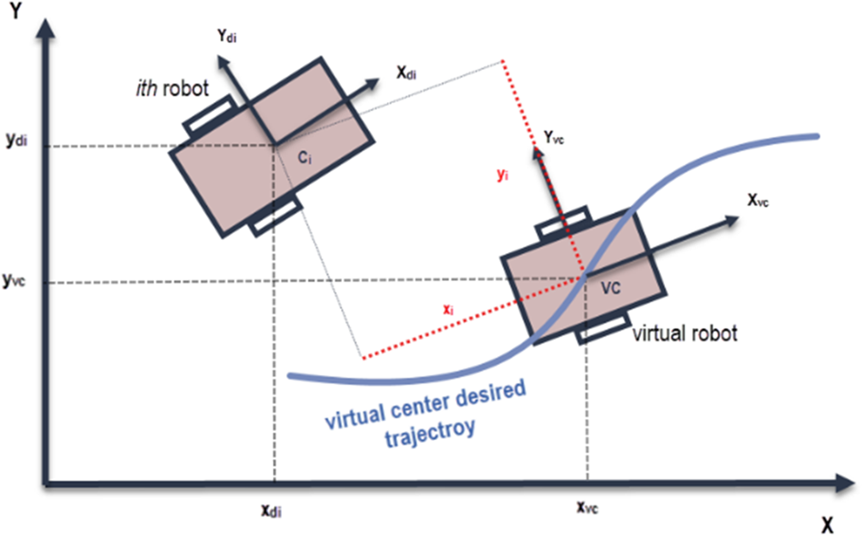
By defining the desired position, orientation, and velocities of the VC in the fixed coordinate frame ${x_{vc}},{y_{vc}}$ [Reference Abbaspour, Moosavian and Alipour20], the desired position for each robot can be easily derived by the following equation

(18) \begin{align}\left[ {\begin{array}{*{20}{c}}{{x_{di}}}\\{{y_{di}}}\end{array}} \right] = \left[ {\begin{array}{*{20}{c}}{{x_{vc}}}\\{{y_{vc}}}\end{array}} \right] + \left[ {\begin{array}{*{20}{c@{\quad}c}}{{\textrm{cos}}{\varphi _{vc}}} & {}{ - {\textrm{sin}}{\varphi _{vc}}}\\{{\textrm{sin}}{\varphi _{vc}}} {}& {{\textrm{cos}}{\varphi _{vc}}}\end{array}} \right]\left[ {\begin{array}{*{20}{c}}{{x_i}}\\{{y_i}}\end{array}} \right]\end{align}

where ${x_i},\;{y_i}$ are two parameters that give the formation its desired shape, and ${x_{di}},\;{y_{di}}$ are the desired position of the i-th robot, see Fig. 3. The formation parameters can be time-varying for flexible formation shapes. Moreover, the desired orientation of each robot ${\varphi _{di}}$ is obtained using the kinematic constraint equation, Eq. 1.

Fig. 3.

The VC concept.

3.2. Path planning and obstacle avoidance

In the presence of obstacles, it is necessary to plan motions that enable the robot to reach the goal without colliding with them. An effective method for achieving that is the use of APFs. The total field is obtained by an attractive potential to the goal and repulsive potentials from the obstacles [Reference Spong, Hutchinson and Vidyasagar35]. As a result, the robot moves in configuration space under the influence of the total potential ${U_{total}}$ . To this end, at each robot configuration, the potential creates an artificial force equal to the negative of the gradient of the total potential which is obtained as a velocity input to the dynamic system of the VC. Therefore, the artificial force specifies the direction and the velocity of the VC planned motion.

As mentioned earlier, the total potential field ${U_{total}}\left( {{{{\textbf{q}}}_{vc}}} \right)$ is a combination of the attractive and the repulsive fields as follows

(19) \begin{align}{U_{total}}\left( {{{{\textbf{q}}}_{vc}}} \right) = {U_{att}}\left( {{{{\textbf{q}}}_{vc}}} \right) + {U_{rep}}\left( {{{{\textbf{q}}}_{vc}}} \right)\end{align}

where ${U_{att}}\left( {{{{\textbf{q}}}_{vc}}} \right)$ is the attractive field and ${U_{rep}}\left( {{{{\textbf{q}}}_{vc}}} \right)$ is the repulsive field. The attractive and repulsive functions used in this paper are defined based on the new potential function proposed in [Reference Ge and Cui36]. The new repulsive functions are introduced by considering the relative distance between the robot and the goal in the calculation of the repulsive field. This approach was inspired by the fact that if the repulsive potentials converge to zero as the robot approaches the goal, then the goal will be at the global minimum.

The attractive and repulsive fields are given in the following equations:

(20) \begin{align}{U_{att}} = \frac{1}{2}\xi {\rho _g}^2\end{align}

(21) \begin{align}{U_{rep}} = \left\{ {\begin{array}{*{20}{c@{\quad}l}}{\frac{1}{2}\eta {{\left( {\dfrac{1}{{{\rho _{ob}}}} - \dfrac{1}{{{\rho _0}}}} \right)}^2}{\rho _g}^n} {}& {{\rho _{ob}} \le {\rho _0}}\\0 {}& {{\rho _{ob}} \gt {\rho _0}}\end{array}} \right.\end{align}

where $\xi $ is a positive scaling parameter, $\eta $ is a positive scaling parameter, ${\rho _g}$ is the distance between the VC and the goal point, ${\rho _{ob}}$ is the distance between the VC and the obstacle, and. ${\rho _0}$ is chosen to be the minimum acceptable distance between the VC and the obstacle. To ensure that none of the robots of the formation collide with the obstacles, ${\rho _0}$ is determined as:

(22) \begin{align}{\rho _0} = R + {r_{obs}}\end{align}

where ${r_{obs}}$ is the obstacle radius including the radius of the largest robot in the system and $R$ is the radius of the formation which indicates the longest distance between the robots to the VC, which can be calculated using the following equation:

(23) \begin{align}R = max{\left\{ {\sqrt {{x_i}^2 + {y_i}^2} } \right\}_{i = 1:n}}\end{align}

where $n$ is the total number of robots. The path planning problem here can be solved as an optimization problem by finding the global minimum in the total field ${U_{total}}$ starting from the initial configuration ${{{\textbf{q}}}_{vc}}\left( {{t_0}} \right).$ The solution to this problem can be given by gradient descent. Thus, the desired velocity of the VC can be considered to be proportional to the negative of the gradient of ${U_{total}}\left( {{{{\textbf{q}}}_{vc}}} \right)$ as

(24) \begin{align}{{{\textbf{v}}}_{vc}} = - K\nabla {{{{\textbf{U}}}}_{total}}\left( {{{{\textbf{q}}}_{vc}}} \right)\end{align}

where K is a positive constant.

4. Controller Design

4.1. Control strategy

The virtual structure approach has been implemented; therefore, the problem of formation control has been replaced with a problem of trajectory tracking. This means that if every robot of the group succeeds in tracking its trajectory, then the formation will be kept as desired. To this end, the MPC-based controllers are designed to solve the problem of trajectory tracking of a group of robots and formation maintenance. The cost function of each robot has a traditional formula that guarantees trajectory tracking. To guarantee formation maintenance in case that one or more of the robots is suffering from disturbance, an extra term is added to the cost function of the proposed controller for each robot. This term contains formation feedback from all other robots. In this way, the formation will be maintained even though some robots are disturbed by external disturbance.

First, the desired trajectory of the VC is generated according to its initial position, its goal, and the locations of the obstacles using APFs. In fact, the velocity of the VC is obtained using Eq. 24; then by the integration of it, the reference trajectory can be found. Next, each individual robot derives its own trajectory using Eq. 18. The next level is the control design where the dynamic equation of the robot is utilized to calculate the torques required to track the trajectory. That will be the first part of the cost function. The second part could use the information from other robots to maintain the formation shape which can be guaranteed by using a new cost function as follows

(25) \begin{align}{J_{total}}^i = {J_t}^{} + {J_f}^i\end{align}

where the sub-index i indicates the i-th robot, with $i\; = 1,2,\; \ldots \;n$ , ${J_{total}}^i$ is the total cost function, ${J_t}^i$ is the part of the cost function that guarantees the trajectory tracking, and ${J_f}^i$ is the part of the cost function that guarantees the formation maintenance. In the following, the control required to solve the problem of trajectory tracking and formation maintenance for a single robot is presented. Two different controllers are designed using the proposed control method as follows.

4.2. Linear model predictive control

Model predictive control systems are designed based on the mathematical model of the plant [Reference Wang37, Reference Camacho and Bordons38]. A state-space model is usually used to represent the control law. In [Reference Loehning, Reble, Hasenauer, Yu and Allgoewer39], a reduced-order model is proposed to control a high-dimensional linear system. Many papers, for example, [Reference Mayne40, Reference Magni, De Nicolao, Scattolini and Allgöwer41], provide different approaches to solve the problem of feedback MPC. The survey paper [Reference Mayne42] states some developments and achievements in MPC.

The main objective of the LMPC here is to track a reference trajectory ${{{\textbf{x}}}_r}(t)$ . In this case, the control algorithm is designed based on the linearization of the system around the desired trajectory ${{{\textbf{x}}}_r}(t)$ . To this end, the Taylor series expansion [Reference Farrell and Polycarpou43] of the system given by Eq. 16 is obtained around the desired trajectory $({{{\textbf{x}}}_r}(t),{{{\textbf{u}}}_r}(t))$ such that

(26) \begin{align}{\dot{\textbf{x}}} = {{\textbf{F}}}({{{\textbf{x}}}_r},{{{\textbf{u}}}_r}) + {\left. {\frac{{\partial {{\textbf{F}}}({{{\textbf{x}}},{{\textbf{u}}}})}}{{\partial {{\textbf{x}}}}}} \right|_{\begin{array}{*{20}{c}}{\textbf{x} = {{{\textbf{x}}}_r}}\\{\textbf{u} = {{{\textbf{u}}}_r}}\end{array}}}({{{\textbf{x}}} - {{{\textbf{x}}}_r}}) + {\left. {\frac{{\partial {{\textbf{F}}}({{{\textbf{x}}},{{\textbf{u}}}})}}{{\partial {{\textbf{u}}}}}} \right|_{\begin{array}{*{20}{c}}{x = {x_r}}\\{u = {u_r}}\end{array}}}\left( {{{\textbf{u}}} - {{{\textbf{u}}}_r}} \right) + \mathcal{F}\end{align}

where ${\mathcal{F}}$ contains the high order terms of the expansion which can be ignored in linear approximations. Therefore, system Eq. 16 after the linearization around the nominal trajectory ${{{\textbf{x}}}_r}(t)$ is expressed in the following form

(27) \begin{align}{{\dot{\textbf{X}}}_e} = {{{\textbf{A}}}_c}(t){{{\textbf{X}}}_{{\textbf{e}}}} + {{{\textbf{B}}}_c}(t){{{{\textbf{U}}}}_{{\textbf{e}}}}\end{align}

where ${{{\textbf{X}}}_{{\textbf{e}}}}$ is the error vector of state variables, ${{{{\textbf{U}}}}_{{\textbf{e}}}}$ is the error vector of control variables with respect to the reference trajectory $({{{\textbf{x}}}_r}(t),{{{\textbf{u}}}_r}(t))$ , and the matrices ${{{\textbf{A}}}_c}(t)$ and ${{{\textbf{B}}}_c}(t)$ are defined as follows

(28) \begin{align}{{{\textbf{A}}}_c}(t) = {\left. {\frac{{\partial {{\textbf{F}}}({{{\textbf{x}}},{{\textbf{u}}}})}}{{\partial {{\textbf{x}}}}}} \right|_{\begin{array}{*{20}{c}}{\textbf{x} = {{{\textbf{x}}}_r}}\\{\textbf{u} = {{{\textbf{u}}}_r}}\end{array}}},{{{\textbf{B}}}_c}(t) = {\left. {\frac{{\partial {{\textbf{F}}}({{{\textbf{x}}},{{\textbf{u}}}})}}{{\partial {{\textbf{u}}}}}} \right|_{\begin{array}{*{20}{c}}{\textbf{x} = {{{\textbf{x}}}_r}}\\{\textbf{u} = {{{\textbf{u}}}_r}}\end{array}}}\end{align}

For simplicity of the framework and the advantage of using the classical linear quadratic regulator, the state-space model in discrete time is used. The state-space form of the system equation in discrete time can be described as follows [Reference Wang37]

(29) \begin{align}{{{\textbf{x}}}_m}({k + 1}) = {{{\textbf{A}}}_m}{{{\textbf{x}}}_m}(k) + {{{\textbf{B}}}_m}{{\textbf{u}}}(k)\end{align}

(30) \begin{align}{{\textbf{y}}}(k) = {{{\textbf{C}}}_m}{{{\textbf{x}}}_m}(k)\end{align}

where u is the manipulated variable or input variable, the matrices ${{{\textbf{A}}}_m},\;{{{\textbf{B}}}_{m,}}$ and ${{{\textbf{C}}}_m}$ are the space state matrices in discrete time, y is the process output, and ${{{\textbf{x}}}_m}$ is the state variable vector with assumed dimension m. Taking a difference operation on both sides of Eq. 29 yields

(31) \begin{align}{{{\textbf{x}}}_m}({k + 1}) - {{{\textbf{x}}}_m}(k) = {{{\textbf{A}}}_m}({{{{\textbf{x}}}_m}(k) - {{{\textbf{x}}}_m}({k - 1})}) + {{{\textbf{B}}}_m}({{{\textbf{u}}}(k) - {{\textbf{u}}}({k - 1})})\end{align}

By defining the incremental of a variable ${{\textbf{v}}}(k)$ by:

\begin{align*}\Delta {{\textbf{v}}}(k) = {{\textbf{v}}}(k) - {{\textbf{v}}}({k - 1})\end{align*}

Eq. 31 can be rewritten as:

(32) \begin{align}\Delta {{{\textbf{x}}}_m}({k + 1}) = {{{\textbf{A}}}_m}\Delta {{{\textbf{x}}}_m}(k) + {{{\textbf{B}}}_m}\Delta {{\textbf{u}}}(k)\end{align}

(33) \begin{align}\Delta {{\textbf{y}}}({k + 1}) = {{{\textbf{C}}}_m}{{{\textbf{A}}}_m}\Delta {{{\textbf{x}}}_m}(k) + {{{\textbf{C}}}_m}{{{\textbf{B}}}_m}\Delta {{\textbf{u}}}(k)\end{align}

where $\Delta {{\textbf{u}}}(k)$ is the input to the incremental state-space model.

By choosing the following new state vector:

(34) \begin{align}{{\textbf{x}}}(k) = {\left[ {\begin{array}{*{20}{c}}{\Delta {{{\textbf{x}}}_m}{{(k)}^T}}\quad {}{{{\textbf{y}}}{{(k)}^T}}\end{array}} \right]^T}\end{align}

and noticing that: $\Delta {{\textbf{y}}}({k + 1}) = {{\textbf{y}}}({k + 1}) - {{\textbf{y}}}(k)$ , the system in Eq. 32, 33 can be represented as:

(35) \begin{align}\begin{array}{*{20}{c}}{\left[ {\begin{array}{*{20}{c}}{\Delta {{{\textbf{x}}}_m}({k + 1})}\\{{{\textbf{y}}}({k + 1})}\end{array}} \right] = \left[ {\begin{array}{*{20}{l@{\quad}l}}{{{{\textbf{A}}}_m}} & {}{\textbf{0}_m^T}\\{{{{\textbf{C}}}_m}_m} & {}{{{{\textbf{I}}}_{q \times q}}}\end{array}} \right]\left[ {\begin{array}{*{20}{c}}{\Delta {{{\textbf{x}}}_m}(k)}\\ {{{\textbf{y}}}(k)}\end{array}} \right] + \left[ {\begin{array}{*{20}{c}}{{{{\textbf{B}}}_m}}\\{{{{\textbf{C}}}_m}{{{\textbf{B}}}_m}}\end{array}} \right]\Delta {{\textbf{u}}}(k)}\\[10pt] {{{\textbf{y}}}(k) = \left[ {\begin{array}{*{20}{c}}{{\textbf{0}_{q \times m}}}\;\;\;\;\; {}{{{{\textbf{I}}}_{q \times q}}}\end{array}} \right]\left[ {\begin{array}{*{20}{c}}{\Delta {{{\textbf{x}}}_m}(k)}\\{{{\textbf{y}}}(k)}\end{array}} \right]}\end{array}\end{align}

where q is the number of outputs. For simplicity, Eq. 35 can be rewritten as follows:

(36) \begin{align}\begin{array}{*{20}{c}}{{{{\textbf{x}}}_a}({k + 1}) = {{{\textbf{A}}}_a}{{{\textbf{x}}}_a}(k) + {{{\textbf{B}}}_a}\Delta {{\textbf{u}}}(k)}\\[4pt] {{{\textbf{y}}}(k) = {{{\textbf{C}}}_a}{{\textbf{x}}}(k)}\end{array}\end{align}

Consider the following vectors at the sampling instant ${k_i},\;{k_i} \gt 0$ :

(37) \begin{align}\Delta {{{\textbf{U}}}} = {\left[\! {\begin{array}{*{20}{c}}{\Delta {{\textbf{u}}}{{\left( {{k_i}} \right)}^T}}\quad {}{\Delta {{\textbf{u}}}{{\left( {{k_i} + 1} \right)}^T}}\quad {}{\begin{array}{*{20}{c}} \ldots\quad {}{\Delta {{\textbf{u}}}{{\left( {{k_i} + {N_c} - 1} \right)}^T}}\end{array}}\end{array}}\! \right]^T}\end{align}

(38) \begin{align}{{\textbf{Y}}} = {\left[\! {\begin{array}{*{20}{c}}{{{\textbf{y}}}{{\left( {{k_i} + 1|{k_i}} \right)}^T}}\quad {}{{{\textbf{y}}}{{\left( {{k_i} + 2|{k_i}} \right)}^T}}\quad {}{\begin{array}{*{20}{c}} \ldots\quad {}{{{\textbf{y}}}{{\left( {{k_i} + {N_p}|{k_i}} \right)}^T}}\end{array}}\end{array}}\!\! \right]^T}\end{align}

where ${{\textbf{y}}}\left( {{k_i} + l|{k_i}} \right)$ is the predicted value of the output ${{\textbf{y}}}$ at ${k_i} + l$ with the given current information ${{{\textbf{x}}}_a}\left( {{k_i}} \right)$ . N _c is the control horizon standing for the number of parameters used to calculate the future control trajectory. This means that the future control variables are predicted for the N _c number of samples. N _p is the predictive horizon which indicates the optimization window. N _p is also the number of future state variables predictions at each sampling instant ${k_i}$ given the current information ${{{\textbf{x}}}_a}({{k_i}})$ . The control horizon is always less than or equal to the prediction horizon; ${N_c} \le {N_p}$ .

After certain calculations, the vector Y is obtained as:

(39) \begin{align}{{\textbf{Y}}} = {{\textbf{F}}}{{{\textbf{x}}}_a}\left( {{k_i}} \right) + {\boldsymbol{\Phi }}{{\Delta }}{{{\textbf{U}}}}\end{align}

where

(40) \begin{align}{{\textbf{F}}} = \left[ {\begin{array}{*{20}{c}}{{{{\textbf{C}}}_a}{{{\textbf{A}}}_a}}\\[4pt]{{{{\textbf{C}}}_a}{{{\textbf{A}}}_a}^2}\\[4pt]{{{{\textbf{C}}}_a}{{{\textbf{A}}}_a}^3}\\ \vdots \\{{{{\textbf{C}}}_a}{{{\textbf{A}}}_a}^{{N_p}}}\end{array}} \right]\end{align}

(41) \begin{align}{\boldsymbol{\Phi }} = \left[ {\begin{array}{*{20}{c@{\quad}c@{\quad}c@{\quad}c@{\quad}c}}{{{{\textbf{C}}}_a}{{{\textbf{B}}}_a}} & {}\textbf{0} {}& \textbf{0} & {} \cdots & {}\textbf{0}\\{{{{\textbf{C}}}_a}{{{\textbf{A}}}_a}{{{\textbf{B}}}_a}} & {}{{{{\textbf{C}}}_a}{{{\textbf{B}}}_a}} & {}\textbf{0} {}& \cdots & {}\textbf{0}\\{{{{\textbf{C}}}_a}{{{\textbf{A}}}_a}^2{{{\textbf{B}}}_a}} & {}{{{{\textbf{C}}}_a}{{\textbf{A}}}{{{\textbf{B}}}_a}} {}& {{{{\textbf{C}}}_a}{{{\textbf{B}}}_a}} {}& \cdots & {}\textbf{0}\\ \vdots {}& \vdots & {} \vdots {}& \ddots & {} \vdots \\{{{{\textbf{C}}}_a}{{{\textbf{A}}}_a}^{{N_p} - 1}{{{\textbf{B}}}_a}} & {}{{{{\textbf{C}}}_a}{{{\textbf{A}}}_a}^{{N_p} - 2}{{{\textbf{B}}}_a}} {}& {{{{\textbf{C}}}_a}{{{\textbf{A}}}_a}^{{N_p} - 3}{{{\textbf{B}}}_a}} {}& \cdots & {}{{{{\textbf{C}}}_a}{{{\textbf{A}}}_a}^{{N_p} - {N_c}}{{{\textbf{B}}}_a}}\end{array}} \right]\end{align}

The main objective of using the LMPC is to make the predictive output close enough or approximately equal to the setpoint signal which can be time-varying in the meaning of a reference trajectory. Therefore, the problem is translated to find the optimal solution for the control vector ${{\Delta }}{{{\textbf{U}}}}$ such that the error between the predictive output and its desired trajectory converges towards zero.

The problem here is a combination of trajectory tracking and formation keeping. To this end, the proposed cost function in Eq. 25 is used to achieve both trajectory tracking and formation keeping objective subject to inequality constraints:

(42) \begin{align}\begin{array}{*{20}{c}}{\begin{array}{*{20}{c}}{\left| {\tau _r^i} \right| \le {\tau _{max}}}\\[5pt] {\left| {\tau _l^i} \right| \le {\tau _{max}}}\end{array}}\\[14pt] {\begin{array}{*{20}{c}}{\left| {\dot \theta _r^i} \right| \le {{\dot \theta }_{max}}}\\[5pt] {\left| {\dot \theta _l^i} \right| \le {{\dot \theta }_{max}}}\end{array}}\end{array}\end{align}

where ${\tau _{max}}$ is the maximum torque of the right and left wheels and ${\dot \theta _{max}}$ is the maximum angular velocity of the right and left wheels. The trajectory tracking cost function for the i-th robot is defined by

(43) \begin{align}{J_t}^i = {{{\textbf{E}}}_t}{}^{i^{T}}{{\textbf{q}}}{{{\textbf{E}}}_t}^i + \Delta {{{{\textbf{U}}}}^{i}}^T{{\textbf{R}}}\Delta {{{{\textbf{U}}}}^i}\end{align}

where $i = 1,2, \ldots ,n$ , Q is a positive-definite weighting matrix, R is a positive semi-definite weighting matrix and $\Delta {{{{\textbf{U}}}}^i}$ is the control increment for the i-th robot, ${{{\textbf{E}}}_t}^i$ is the tracking error for the i-th robot which is represented as

(44) \begin{align}{{{\textbf{E}}}_t}^i = {{{\textbf{R}}}_s}^i - {{{\textbf{F}}}^i}{{{\textbf{x}}}_a}^{i}({{k_m}})\end{align}

where ${{{\textbf{R}}}_s}^i$ is an $\left( {N \times m} \right) \times 1\;$ vector that contains the setpoint information for an N step for the i-th robot, and ${{{\textbf{F}}}^i}$ is defined by Eq. 40 for the i-th robot.

In addition, the formation keeping cost function is described as

(45) \begin{align}{J_f}^i = \sum{}_{\substack{j = 1 \\ j \ne i}}^n {{{\textbf{E}}}_{f,j}}{{}^{i^{T}}}{{\textbf{P}}}{{{\textbf{E}}}_{f,j}}^i\end{align}

where P is a positive-definite diagonal weighting matrix and ${{{\textbf{E}}}_{f,j}}^i$ is the quasi-formation error between the i-th and the j-th robots and is obtained as

(46) \begin{align}{{{\textbf{E}}}_{f,}}^i = \sum{}_{\substack{j = 1 \\ j \ne i}}^n \left( {\left( {{{{\textbf{F}}}^j}{{{\textbf{x}}}_a}^{j}({{k_m}}) - {{{\textbf{F}}}^i}{{{\textbf{x}}}_a}^{i}({{k_m}})} \right) - \left( {{{{\textbf{R}}}_s}^j - {{{\textbf{R}}}_s}^i} \right)} \right)\end{align}

The total cost function can be rewritten in the following form

(47) \begin{align}J & = \Delta {{{{\textbf{U}}}}^{i^T}}\!({{{\boldsymbol{\Phi }}^{i^T}}{{\textbf{q}}}{{\boldsymbol{\Phi }}^i} + {{\textbf{R}}} + (n - 1){{\boldsymbol{\Phi }}^{i^T}}{{\textbf{P}}}{{\boldsymbol{\Phi }}^i}}){{\Delta }}{{{{\textbf{U}}}}^i} - 2{\left( {{{{\textbf{R}}}_s}^i - {{{\textbf{F}}}^i}{{{\textbf{x}}}^i}({{k_m}})} \right)^T}{{\textbf{q}}}{{\boldsymbol{\Phi }}^i}\Delta {{{{\textbf{U}}}}^i} \nonumber\\ & \quad + {\left( {{{{\textbf{R}}}_s}^i - {{{\textbf{F}}}^i}{{{\textbf{x}}}^i}\left( {{k_m}} \right)} \right)^T}{{\textbf{q}}}\left( {{{{\textbf{R}}}_s}^i - {{{\textbf{F}}}^i}{{{\textbf{x}}}^i}\left( {{k_m}} \right)} \right) + \sum{}_{\substack{j = 1 \\ j \ne i}}^n \!\!\left(\!{-2{{\textbf{E}}}{{_{f,j}^{i}}}^T{{\textbf{P}}}{{\boldsymbol{\Phi }}^i}\Delta {{{{\textbf{U}}}}^i} + {{\textbf{E}}}{{_{f,j}^{i}}}^T{{\textbf{PE}}}_{f,j}^i} \right)\end{align}

where ${{\boldsymbol{\Phi }}^i}$ is defined by Eq. 41 for the i-th robot. Finding the optimal control signal $\Delta {{{\textbf{U}}}}$ that minimizes the cost function in Eq. 47 subject to the constraints in Eq. 42 is a quadratic programming problem [Reference Wang37]. Hence, the cost function to minimize is written as follows

(48) \begin{align}\begin{array}{*{20}{c}}{{J^i} = \dfrac{1}{2}\Delta {{{{\textbf{U}}}}^{i^T}}{{{\textbf{H}}}^{{\textbf{i}}}}\Delta {{{{\textbf{U}}}}^i} + {{{\textbf{f}}}^{i^T}}\Delta {{{{\textbf{U}}}}^i} + {r^i}}\\[5pt] {S.t\, \, \, \, \, \;{{{\textbf{M}}}^i}\Delta {{{{\textbf{U}}}}^i} \le {{\boldsymbol{\gamma }}^i}}\end{array}\end{align}

where

\begin{align*}{{{\textbf{H}}}^i} = 2\left( {{{\boldsymbol{\Phi }}^{i^T}}{{\textbf{q}}}{{\boldsymbol{\Phi }}^i} + {{\textbf{R}}} + (n - 1){{\boldsymbol{\Phi }}^{i^T}}{{\textbf{P}}}{{\boldsymbol{\Phi }}^i}} \right)\;,\, \, \, \, \, \, \, \, \, \, \, \, \, \, \, \, \, \, \, \, \, \, \, \, \, \;\;\;\;\end{align*}

\begin{align*}{{{\textbf{f}}}^{i^T}} = - 2{\left( {{{{\textbf{R}}}_s}^i - {{{\textbf{F}}}^i}{{{\textbf{x}}}^i}\left( {{k_m}} \right)} \right)^T}{{\textbf{q}}}{{\boldsymbol{\Phi }}^i} - \mathop \sum \limits_{\substack{j = 1 \\ j \ne i}}^n 2{{\textbf{E}}}{_{f,j}^{i}}^T{{\textbf{P}}}{{\boldsymbol{\Phi }}^i},\, \, \, \, \, \, \, \, \, \, \, \, \, \, \, \end{align*}

\begin{align*}{r^i} = {\left( {{{{\textbf{R}}}_s}^i - {{{\textbf{F}}}^i}{{{\textbf{x}}}^i}\left( {{k_m}} \right)} \right)^T}{{\textbf{q}}}\left( {{{{\textbf{R}}}_s}^i - {{{\textbf{F}}}^i}{{{\textbf{x}}}^i}\left( {{k_m}} \right)} \right) + \mathop \sum \limits_{\substack{j = 1 \\ j \ne i}}^n {{\textbf{E}}}{_{f,j}^{i}}^T{{\textbf{PE}}}_{f,j}^i\end{align*}

${{{\textbf{M}}}^i}$ is a matrix reflecting the constraints in Eq. 38 which are written in terms of $\Delta {{{{\textbf{U}}}}^i}$ , ${{\boldsymbol{\gamma }}^i}$ is a vector representing the limits of the constrained variables, and ${r^i}$ is a constant. It is worth noting that terms that do not contain $\Delta {{{{\textbf{U}}}}^i}$ can be treated as constant. In this work, the “quadprog” solver in MATLAB software was used to solve this linear quadratic programming problem.

4.3. Nonlinear model predictive control

NMPC is a strategy for constrained feedback control of nonlinear systems. The basic idea of the linear and nonlinear model predictive control is to predict and optimize the future behavior using the model of the system [Reference Camacho and Bordons38, Reference Lars and Jürgen44, Reference Maciejowski45].

For the simplicity and the advantage of using the classical linear quadratic regulator purposes, the system model in discrete time is used. The nonlinear state-space model described in Eq. 16 can be written in discrete time as follows

(49) \begin{align}{{\textbf{x}}}({k + 1}) = {{{\textbf{f}}}_d}({t,{{\textbf{x}}}(k),{{\textbf{u}}}(k)})\end{align}

and the reference trajectory in discrete time is

(50) \begin{align}{{{\textbf{x}}}_r}({k + 1}) = {{{\textbf{f}}}_r}\left( {{{{\textbf{x}}}_r},{{{\textbf{u}}}_r}} \right)\end{align}

Hence, the predictive state of the robot is obtained as

(51) \begin{align}{{\textbf{x}}}({k + j + 1{\textrm{|}}k}) = {{{\textbf{f}}}_d}({{{\textbf{x}}}({k + j{\textrm{|}}k}),{{\textbf{u}}}({k + j{\textrm{|}}k})})\end{align}

where for an arbitrary variable ${{\textbf{z}}}$ , ${{\textbf{z}}}({k + j{\textrm{|}}k})$ indicates the value of variable ${{\textbf{z}}}$ predicted at the $k + j$ instant given the current information ${{\textbf{z}}}(k)$ .

The optimization problem is solved at every sampling time where the control sequence u each time is derived to bring the states close to the reference trajectory. The same total cost function in Eq. 25 is rewritten as

(52) \begin{align}{J_{N,total}}^i = \mathop \sum \limits_{j = 1}^{Np} {l^i}({t,{{{\textbf{e}}}^i}(j),{{{\bar{\textbf{u}}}}^i}(j)}) + {G^i}({{{{\textbf{e}}}^i}({{N_p}})})\end{align}

where ${J_{N,total}}^i$ is the total cost function for the NMPC, ${l^i}({t,{{{\textbf{e}}}^i}(j),{{{\bar{\textbf{u}}}}^i}(j)}) = {J_{N,t}}^i + {J_{N,f}}^i$ , the first term ${J_{N,t}}^i$ is the part of the control that leads the i-th robot to follow its desired trajectory, ${J_{N,f}}^i$ is the other part of the control that guarantees formation keeping, and ${G^i}$ is the terminal cost function which is added to guarantee the stability of the closed-loop system. Also, ${{\bar{\textbf{u}}}^i}$ is the error vector of control input with respect to its reference value. The trajectory tracking cost function for the i-th robot is defined as

(53) \begin{align}{J_{N,t}}^i({{{{\textbf{e}}}^i}(j),{{{\bar{\textbf{u}}}}^i}(j)}) = {{{\textbf{e}}}^{i^T}}({k + j{\textrm{|}}k}){{{\textbf{Q}}}_N}{{{\textbf{e}}}^i}({k + j{\textrm{|}}k}) + {{\bar{\textbf{u}}}^{i^T}}\!({k + j{\textrm{|}}k}){{{\textbf{R}}}_N}{{\bar{\textbf{u}}}^i}({k + j{\textrm{|}}k})\end{align}

where ${{{\textbf{Q}}}_N}$ is a positive-definite weighting matrix, ${{{\textbf{R}}}_N}$ is a positive semi-definite weighting matrix, N is the prediction horizon which indicates the number of future variables predictions at each sampling instant ${k_i}$ given the current information $x({{k_i}})$ , and ${{{\textbf{e}}}^i}({k + j{\textrm{|}}k})$ is the tracking error for the i-th robot represented as

(54) \begin{align}{{{\textbf{e}}}^i}({k + j{\textrm{|}}k}) = {{\textbf{x}}}({k + j{\textrm{|}}k}) - {{{\textbf{x}}}_r}({k + 1})\end{align}

Moreover, the formation maintaining part of the cost function is obtained as follows

(55) \begin{align}{J_{N,f}}^i({t,{{{\textbf{e}}}^i}(j)}) = \mathop \sum{}_{\substack{l = 1 \\ l \ne i}}^n {{{\textbf{e}}}_{f,l}}{^{i^T}}({k + j{\textrm{|}}k}){{{\textbf{P}}}_N}{{{\textbf{e}}}_{f,l}}^i({k + j{\textrm{|}}k})\end{align}

where ${{{\textbf{P}}}_N}$ is a positive-definite diagonal weighting matrix and ${{{\textbf{e}}}_{f,l}}^i({k + j{\textrm{|}}k})$ is the quasi-formation error between the i-th robot and l-th robot which can be defined as

(56) \begin{align}{{{\textbf{e}}}_{f,l}}^i({k + j{\textrm{|}}k}) = \left( {{{{\textbf{x}}}^i}({k + j{\textrm{|}}k}) - {{{\textbf{x}}}^l}({k + j{\textrm{|}}k})} \right) - \left( {{{\textbf{x}}}_d^i({k + j{\textrm{|}}k}) - {{\textbf{x}}}_d^l({k + j{\textrm{|}}k})} \right)\end{align}

The terminal cost function is chosen as a positive-definite function as follows:

\begin{align*}{G^i}({{{{\textbf{e}}}^i}({{N_p}})}) = {{{\textbf{e}}}^{i^T}}({k + {N_p}{\textrm{|}}k}){{{\textbf{L}}}_N}{{{\textbf{e}}}^i}({k + {N_p}{\textrm{|}}k})\end{align*}

where ${{{\textbf{L}}}_N}$ is a positive-definite diagonal weighting matrix. The optimal control problem is chosen as

(57) \begin{align}{V^{{i^*}}} = {J_{NMPC,oal}}^i\end{align}

subject to

(58) \begin{align} {{{\textbf{x}}}^i}({k + j + 1{\textrm{|}}k}) = {{\textbf{f}}}_d^i( {{{{\textbf{x}}}^i}({k + j{\textrm{|}}k})} &+ {{{{\textbf{u}}}^i}({k + j{\textrm{|}}k})}),for\;j = 0, \ldots ,{N_p} \nonumber \\ \left| {\tau _r^i} \right| & \le {\tau _{max}} \nonumber \\\left| {\tau _l^i} \right| & \le {\tau _{max}} \nonumber \\ \left| {\dot \theta _r^i} \right| & \le {{\dot \theta }_{max}} \\\left| {\dot \theta _l^i} \right| & \le {{\dot \theta }_{max}} \nonumber\\{{\textbf{x}}}(0) & = {{{\textbf{x}}}_0}\nonumber \\ {{{\textbf{x}}}^i}({k}\; +&\; {{N_p}}) \in {{{\mathbb {X}}_f}} \nonumber \end{align}

where ${V^{{i^*}}}$ is the optimal value of the cost function, ${\mathbb {X}_f}$ is the allowable terminal state constraints. The nonlinear optimal problem in Eq. 57 is solved for state ${{{\textbf{x}}}^i}$ at time instant $k$ using the “fmincon” MATLAB solver, and the optimal control sequence is

(59) \begin{align}{{\textbf{u}}}_{\textrm{*}}^i = \left\{ {{{\textbf{u}}}_{\textrm{*}}^i(0),{{\textbf{u}}}_{\textrm{*}}^i\left( 1 \right), \ldots ,{{\textbf{u}}}_{\textrm{*}}^i\left( {{N_p} - 1} \right)} \right\}\end{align}

The associated optimal state is

(60) \begin{align}{{\textbf{x}}}_{\textrm{*}}^i = \left\{ {{{\textbf{x}}}_{\textrm{*}}^i(0),{{\textbf{x}}}_{\textrm{*}}^i\left( 1 \right), \ldots ,{{\textbf{x}}}_{\textrm{*}}^i\left( {{N_p} - 1} \right)} \right\}\end{align}

The model predictive control can be represented as follows

(61) \begin{align}{{\unicode[Times]{x1D6CD} }}_N^i({{\textbf{x}}}) = {{\textbf{u}}}_{\textrm{*}}^i(0)\end{align}

One way of ensuring (or enforcing) stability in MPC-based controllers is to add a terminal constraint that forces the state to assume a particular value at the end of the prediction horizon. [Reference Lars and Jürgen44, Reference Maciejowski45]. The stability analysis of the developed NMPC system is investigated in the Appendix.

5. Formation Evaluation Criteria

To calculate the total formation error, we consider the two following criteria.

1. 1- Distance error between each pair: $\forall \;i,\;j = 1,2, \ldots n\;and\;i \ne j$ , the pair of robots $\left( {{R_i},\;{R_j}} \right)$ inner-robot distance $dist\left( {{R_i},{R_j}} \right) = \sqrt {{{\left( {{x_{{R_i}}} - {x_{{R_j}}}} \right)}^2} + {{\left( {{y_{{R_i}}} - {y_{{R_j}}}} \right)}^2}} $ , and the desired inner-robot distance ${d_{{d_{ij}}}}$ , where $\left( {{x_{{R_i}}},{y_{{R_i}}}} \right)$ is the i-th robot position and $\left( {{x_{{R_j}}},{y_{{R_j}}}} \right)$ is the j-th robot position, we define the distance error between ${R_i}$ and ${R_j}$ as follows: ${e_{{d_{ij}}}} = dist\left( {{R_i},{R_j}} \right) - {d_{{d_{ij}}}}$ . The total distance error between robots can be expressed as follows

(62) \begin{align}{E_{{d_t}}} = \frac{1}{2}\sum\nolimits_{\substack{i,j = 1 \\ i \ne j}}^n {e_{{d_{ij}}}}\end{align}

1. 2- Order error: We can describe the topology of the formation using a directed graph, where the robots represent the vertices of the graph and the relations between the robots represent the directed edges that connect these vertices or nodes. We define the order error ${E_{{o_j}}} = {o_j} - {o_{{j_{des}}}}$ , where ${o_j}$ is a measure of the order of the j-th vertex in the real formation and ${o_{{j_{des}}}}$ is a measure of the order of the j-th vertex in the desired formation. It is possible to determine the order of the robots in the formation by using the outer product of the directed edges of the formation. The sign of the outer product determines the right direction or order of the target vertices. Therefore, ${o_j}$ and ${o_{{j_{des}}}}$ can be defined as $\frac{{{V_{ij}} \times {V_{jk}}}}{{\left| {{V_{ij}} \times {V_{jk}}} \right|}}$ and $\frac{{{V_{i{j_{des}}}} \times {V_{j{k_{des}}}}}}{{\left| {{V_{i{j_{des}}}} \times {V_{j{k_{des}}}}} \right|}}$ , respectively, where ${V_{ij}}$ and ${V_{i{j_{des}}}}$ are the real and desired vectors originating from the i-th robot toward the j-th robot, respectively. Also, ${V_{jk}}$ and ${V_{j{k_{des}}}}$ are the real and desired vectors originating from the j-th robot toward the k-th robot, respectively. The total order error may be written as

(63) \begin{align}{E_{{o_t}}} = \mathop \sum \nolimits_k^n {E_{{o_k}}}\end{align}

One may consider the weighted summation of these two errors to derive the total formation error. The proposed formation error is given as follows

(64) \begin{align}{E_{Total}} = \frac{1}{{{n_{pairs}}}}{E_{{d_t}}} + \alpha {E_{{o_t}}}\end{align}

where ${n_{pairs}}$ is the number of robots’ pairs which is equal to $\frac{n}{2}\left( {n - 1} \right)$ , and $\alpha $ is a user-defined weighting factor.

In order to achieve the desired geometric shape of the formation, the total formation error should approach zero. This can be achieved when the distance between each pair of the robots satisfies the following inner-robot distance condition ${e_{{d_{ij}}}} \cong 0,\;\;\forall i,j = 1,2, \ldots ,n$ and when the robots are in the right order ${E_{{o_j}}} \cong 0,\;\;\forall j = 1,2,\ldots,n$ .

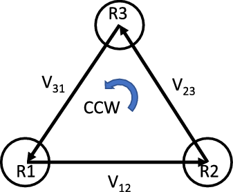
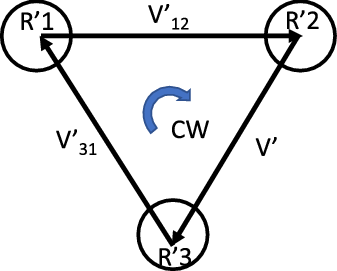
Suppose that we have a system of 3 WMRs. It is obvious that there are two different formations that satisfy the inner-robot distance condition in a two-dimensional space. Figures 4 and 5 show the two possible formations counterclockwise and clockwise, respectively.

Fig. 4.

Counterclockwise formation.

Fig. 5.

Clockwise formation.

For a system with a larger number of robots, the possible formations are more than two. Therefore, these different formations should be taken into account to achieve the desired formation. To this end, the order error defined in criterion 2 for all vertices of the graph is utilized to measure the direction of formation. For instance, take the two formations in Figs. 4 and 5. Assume that the desired formation is shown in Figure 4 and the real one is shown in Fig. 5. With the assumption that the real inner-robot distances are approximately equal to the desired ones, we calculate ${o_{{j_{des}}}},\;{o_j}$ and ${E_{{o_j}}}$ for $j = 1,\;2,\;3$ as follows

\begin{align*} {o_{{1_{des}}}} = \frac{{{V_{{{31}_{des}}}} \times {V_{{{12}_{des}}}}}}{{\left| {{V_{{{31}_{des}}}} \times {V_{{{12}_{des}}}}} \right|}} = 1,\quad {o_1} = \frac{{V'_{\!\!31} \times V'_{\!\!12}}}{{\left| {V'_{\!\!31} \times V'_{\!\!12}} \right|}} = - 1,\quad {E_{{o_1}}} = 2 \end{align*}

Similarly, ${o_{{2_{des}}}} = 1,\;\;{o_2} = - 1,\;\;{E_{{o_2}}} = 2$ and ${o_{{3_{des}}}} = 1,\;\;{o_3} = - 1,\;\;{E_{{o_3}}} = 2$ .

The previous example shows that the robots should satisfy the inner-distance condition; however, this is a necessary but not sufficient condition for formation keeping. The robots should be in the right order as well. Therefore, in addition to the inner-distance measure, the order criterion should be addressed.

6. Simulation

The simulation is accomplished using MATLAB software, where a group of WMRs is navigating from a start point to a goal point. The two controllers have been applied to enable the robots to track their desired trajectories, avoid obstacles, and maintain the desired formation. In order to evaluate the performance of the controllers, two kinds of disturbances are applied to the system, namely constant and harmonic. Four case studies are discussed in the following. Moreover, the results are compared with the feedback linearization and Laguerre MPC methods that are mentioned in the introduction.

Case study 1: illustration of the proposed method with the application of constant disturbance

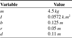
The control approaches discussed in the previous section were successfully simulated using MATLAB software. The system consists of three nonholonomic differential drive WMRs. The three robots are identically the same, and each has the parameters shown in Table I.

Table I.

Single robot properties.

The reference trajectory of the VC is generated using the proposed APF functions. The initial position and orientation of the VC are ${{{\textbf{x}}}_{vc}}({t_0}) = {\left[ {\begin{array}{*{20}{c}}{ - 0.2}\quad {}{ - 1.5}\quad {}0\end{array}} \right]^T}$ , and the goal pose for the VC to reach is ${{{\textbf{x}}}_{vc}}({t=60}) = {\left[ {\begin{array}{*{20}{c}}{2.2}\quad {}{4.8}\quad {}{2.18}\end{array}} \right]^T}$ . The APF parameters are $K = 0.015,\eta = 5.4,\zeta = 8.28$ .

Suppose that the initial velocities of the robots are zeros. The initial position and orientation of each robot are

\begin{align*}{{{\textbf{x}}}_1}({t_0}) = {\left[ {\begin{array}{*{20}{c}}{ - 0.75}\quad {}{ - 1.3975}\quad {}{0.327}\end{array}} \right]^T},\;\;\end{align*}

\begin{align*}{{{\textbf{x}}}_2}({t_0}) = {\left[ {\begin{array}{*{20}{c}}{ - 0.498}\quad {}{ - 2.802}\quad {}{0.799}\end{array}} \right]^T},\;\;\end{align*}

\begin{align*}{{{\textbf{x}}}_3}({t_0}) = {\left[ {\begin{array}{*{20}{c}}{ - 1.685}\quad {}{ - 1.397}\quad {}{0.718}\end{array}} \right]^T}\end{align*}

The desired trajectory of each robot is derived using Eq. 18; the formation parameters ${x_i},{y_i}$ are given as follows

\begin{align*}{x_1} = 0.104,\, \, \, \, \, \;\;\;\;{y_1} = 0.136\end{align*}

\begin{align*}{x_2} = -0.712,\, \, \, \, \, {y_2} = - 0.656\end{align*}

\begin{align*}{x_3} = - 0.88,\, \, \, \, \, \;\;\;{y_3} = 0.88\end{align*}

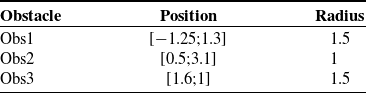
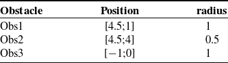
The robots navigate from the initial positions to the goals through 3 obstacles. The position and radius for each obstacle are represented in Table II.

Table II.

Obstacle specifications.

In addition, the APF parameters are $K = 0.015,\eta = 0.69,\zeta = 0.9$ .

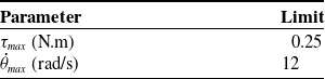
It is worth noting that constraints are designed for both input and state variables. Assume that the maximum linear velocity of each WMR is 0.6 m/s and the maximum output torque of the motor is 0.25 N.m, then the constraints on the wheels’ torques and the wheels’ velocities can be listed in Table III. This was obtained in both cases; however, the results will be shown only for the formation control case and for the first robot only.

Table III.

Constraints on inputs and states.

The three robots are simulated using the previous parameters to perform a triangle formation. Each robot tracks a trajectory given in Eq. 19 without collision with obstacles. In addition, the team of robots should maintain the desired formation even when the system suffers from disturbance. In practice, robots may be exposed to different types of disturbance, such as unwanted external input or actuator fault. To illustrate that, we have supposed that the first robot is experiencing an unwanted input during some parts of its motion. To demonstrate the effectiveness of the proposed control method, two cases are discussed here:

• Case 1.1: the robots use the control method in Eq. 25 without formation control cost function; that is, ${J_f}^i = 0,\;\;for\;i = 1,2,3$

• Case 1.2: the formation control cost function is considered.

The aforementioned disturbance is applied to the first robot in both cases in the time interval [Reference Lee and Chwa25, Reference Spong, Hutchinson and Vidyasagar35] s where the total simulation time is 60 s and the sampling time is ${T_s} = 0.1 \,{\rm{s}}$ . To this end, the torque of the right wheel is multiplied by 0.7, and the torque of the left wheel is multiplied by 0.01.

The prediction horizon and control horizon are tuning parameters. According to [Reference Wang37], the prediction horizon, $Np$ in LMPC and N in NMPC, should be chosen so that it is not too short or too long. Short horizons yield a system that is not necessarily stable. On the other hand, for a large prediction horizon, the system will encounter a numerical stability problem. Therefore, the prediction horizon is selected so that the system has a convenient performance. As for the control horizon, in the case of MPC, we have mentioned before that the control horizon should be less than or equal to the prediction horizon. To this end, a control horizon of 5 is chosen.

The Q and R matrices are tuning parameters that are chosen as a tradeoff between control effort and performance. The weighting matrix R is usually chosen as R = I, where I is the ( $2 \times 2$ ) identity matrix. It is evident that increasing the weights of R will lead to a high control effort and reduce the closed-loop response speed [Reference Wang37]. There are many methods to choose the matrix Q in the literature such as the Riccati equation, Ziegler-Nichols, self-tuning, and manual tuning [Reference Camacho and Bordons38]. Several values for the Q matrix were tested manually before the weights are chosen such that the performance of the control system is acceptable. In order to have a fair comparison between the two controllers, the control parameters for both cases are given as follows

• Case 1.1: without formation control

  MPC

  \begin{align*}{{\textbf{Q}}} = {\textrm{diag}}\left( {\left[\! {\begin{array}{*{20}{c}}{110}\;\;\;\;\; {}{\begin{array}{*{20}{c}}{140}\;\;\;\;\; {}{50}\;\;\;\;\; {}{\begin{array}{*{20}{c}}{0.05}\;\;\;\;\; {}{0.05}\end{array}}\end{array}}\end{array}}\!\! \right]} \right),\;\;{{\textbf{R}}} = {\textrm{diag}}\left( {\left[\! {\begin{array}{*{20}{c}}1\;\;\;\;\; {}1\end{array}}\! \right]} \right),\;\;{{\textbf{P}}} = 0\end{align*}
  \begin{align*}{N_p} = 10,\;\;{N_c} = 5\end{align*}

• NMPC

  \begin{align*}{{{\textbf{Q}}}_N} = {\textrm{diag}}\left( {\left[\! {\begin{array}{*{20}{c}}{110}\;\;\;\;\; {}{\begin{array}{*{20}{c}}{140}\;\;\;\;\; {}{50}\;\;\;\;\; {}{\begin{array}{*{20}{c}}{0.05}\;\;\;\;\; {}{0.05}\end{array}}\end{array}}\end{array}}\!\! \right]} \right),\;\;{{{\textbf{R}}}_N} = {\textrm{diag}}\left( {\left[ \!{\begin{array}{*{20}{c}}1\;\;\;\;\; {}1\end{array}}\! \right]} \right),\;\;{{{\textbf{P}}}_N} = 0,\end{align*}
  \begin{align*}{{{\textbf{L}}}_N} = {\textrm{diag}}\left( {\left[\! {\begin{array}{*{20}{c}}{250}\;\;\;\;\; {}{\begin{array}{*{20}{c}}{250}\;\;\;\;\; {}{0.5}\;\;\;\;\; {}{\begin{array}{*{20}{c}}{0.05}\;\;\;\;\; {}{0.05}\end{array}}\end{array}}\end{array}}\!\! \right]} \right),\;\;{N_p}\; = 10\end{align*}

• Case 1.2: with formation control

  MPC

  \begin{align*}{{\textbf{Q}}} = {\textrm{diag}}\left( {\left[\! {\begin{array}{*{20}{c}}{110}\;\;\;\;\; {}{\begin{array}{*{20}{c}}{140}\;\;\;\;\; {}{50}\;\;\;\;\; {}{\begin{array}{*{20}{c}}{0.05}\;\;\;\;\; {}{0.05}\end{array}}\end{array}}\end{array}}\!\! \right]} \right),\;\;{{\textbf{R}}} = {\textrm{diag}}\left( {\left[ \!{\begin{array}{*{20}{c}}1\;\;\;\;\; {}1\end{array}}\! \right]} \right)\end{align*}
  \begin{align*}{{\textbf{P}}} = {\textrm{diag}}\left( {\left[\! {\begin{array}{*{20}{c}}{20}\;\;\;\;\; {}{\begin{array}{*{20}{c}}{30}\;\;\;\;\; {}8\;\;\;\;\; {}{\begin{array}{*{20}{c}}{0.012}\;\;\;\;\; {}{0.012}\end{array}}\end{array}}\end{array}}\!\! \right]} \right),\;\;\end{align*}
  \begin{align*}{N_p} = 10,\;\;{N_c} = 5.\end{align*}

• NMPC

  \begin{align*}{{{\textbf{Q}}}_N} = {\textrm{diag}}\left( {\left[\! {\begin{array}{*{20}{c}}{110}\;\;\;\;\; {}{\begin{array}{*{20}{c}}{140}\;\;\;\;\; {}{50}\;\;\;\;\; {}{\begin{array}{*{20}{c}}{0.05}\;\;\;\;\; {}{0.05}\end{array}}\end{array}}\end{array}}\!\! \right]} \right),\;\;{{{\textbf{R}}}_N} = {\textrm{diag}}\left( {\left[\! {\begin{array}{*{20}{c}}1\;\;\;\;\; {}1\end{array}}\! \right]} \right)\end{align*}
  \begin{align*}{{{\textbf{P}}}_N} = {\textrm{diag}}\left( {\left[\! {\begin{array}{*{20}{c}}{20}\;\;\;\;\; {}{\begin{array}{*{20}{c}}{30}\;\;\;\;\; {}8\;\;\;\;\; {}{\begin{array}{*{20}{c}}{0.012}\;\;\;\;\; {}{0.012}\end{array}}\end{array}}\end{array}}\!\! \right]} \right),\;\;\end{align*}
  \begin{align*}{{{\textbf{L}}}_N} = {\textrm{diag}}\left( {\left[\! {\begin{array}{*{20}{c}}{250}\;\;\;\;\; {}{\begin{array}{*{20}{c}}{250}\;\;\;\;\; {}{0.5}\;\;\;\;\; {}{\begin{array}{*{20}{c}}{0.05}\;\;\;\;\; {}{0.05}\end{array}}\end{array}}\end{array}}\!\! \right]} \right),\;\;{N_p} = 10\end{align*}

Case 1.1: Without formation control

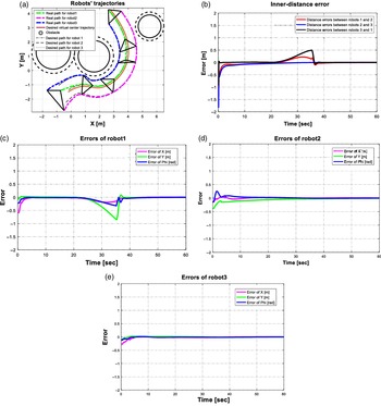
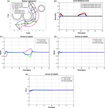
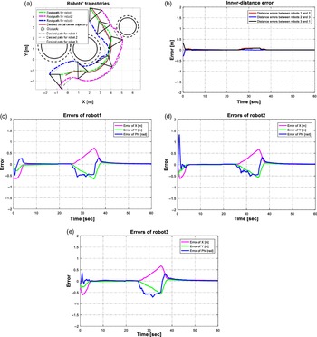
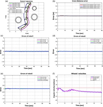
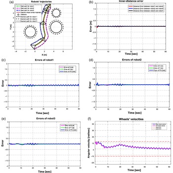
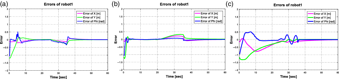
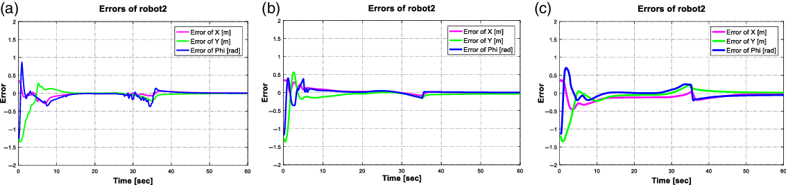
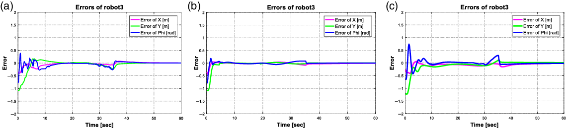
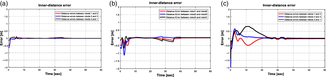
In the first case, when the formation maintaining concept is not taken into consideration in the cost function, the robots do not receive formation feedback from each other. Figures 6 and 7 illustrate the results of simulation LMPC and NMPC, respectively, for the first case. In the absence of disturbance, the three controllers are able to track the trajectories and maintain the formation successfully. It is seen that the robots are in the right order the whole simulation time. However, the simulation results indicate that the distance error between the three robots, for the two controllers, is relatively large in the interval when an external disturbance is exerted on one of the robots. In this interval, as mentioned earlier since there is no feedback information between the robots, the distance error between robots increases and the formation cannot keep the desired shape in the existence of disturbance. Nevertheless, the two controllers have yielded errors that converge to zero.

Fig. 6.

LMPC without formation control. (a) VC and robots’ trajectories. (b) The inner-distance error between the robots. (c) Error signals of robot 1. (d) Errors of robot 2. (e) Errors of robot 3.

Fig. 7.

NMPC without formation control. (a) VC and robots’ trajectories. (b) The inner-distance error between the robots. (c) Error signals of robot 1. (d) Errors of robot 2. (e) Errors of robot 3.

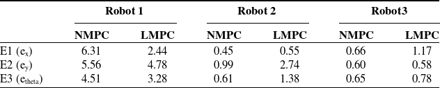
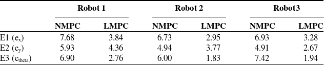
Using the virtual structure formation method can guarantee formation maintenance if all the robots succeed in tracking their desired trajectories. However, if one of the robots experiences disturbance, it will react to the error and try to get back to its desired path. Other robots will continue tracking their own trajectories without having any reaction to the errors of the first robot, and as a result, the formation will fail. The integrated time absolute errors for both controllers are compared and reported in Tables IV and V.

Table IV.

Integrated time absolute error of x, y, and angle, case study 1–1.

Table V.

Integrated time absolute inner-distance error, case study 1–1.

Case 1.2: With formation control

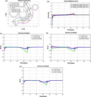
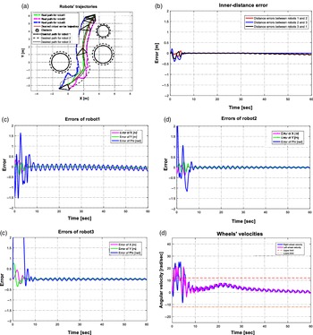
In the second case, when the formation maintaining concept is implemented in the cost function, each robot receives feedback on the location of other robots. This helps the robots compensate for the inner-distance error. In some applications, such as moving an object, the formation task is more important than the trajectory tracking and this is where the importance of such a controller arises even if it causes larger errors in trajectory tracking. Figures 8 and 9 illustrate the results of simulation LMPC and NMPC, respectively, in the presence of formation control. This simulation illustrates that the robots try to maintain the formation rather than tracking the individual trajectories. Figures show that when the first robot has disturbance, the other two robots try to compensate for the inner-distance error which leads to a tracking error, that is, the robots change their paths related to the occurred disturbance to maintain the formation. The integrated time absolute errors for both controllers are compared and reported inTables VI and VII.

Fig. 8.

LMPC in the presence of formation control. (a) VC and robots’ trajectories. (b) The inner-distance error between the robots. (c) Error signals of robot 1. (d) Errors of robot 2. (e) Errors of robot 3.

Fig. 9.

NMPC in the presence of formation control. (a) VC and robots’ trajectories. (b) The inner-distance error between the robots. (c) Error signals of robot 1. (d) Errors of robot 2. (e) Errors of robot 3.

Table VI.

Integrated time absolute error of x, y, and angle, case study 1–2.

Table VII.

Integrated time absolute inner-distance error, case study 1–2.

It can be noticed that the tracking errors of the NMPC are large compared to those of LMPC when the system experiences disturbance. This is because the controller is trying to effectively compensate for the error resulting from the first robot. However, the inner-distance error of the NMPC is extremely small during the period when the system is disturbed. The maximum distance error between the robots of the NMPC is approximately less than 0.1 m, whereas the maximum distance error between the robots for the NMPC case is almost over 0.2 m. Furthermore, the initial inner-distance errors that occurred at the beginning of the simulation for the LMPC are large, while for the NMPC, there are no overshoots or undershoots. Simulation results show that the order error of all robots is zero during the whole simulation time for both controllers. It can be noticed that the tracking errors of NMPC without disturbance converge to zero faster compared with LMPC Therefore, NMPC shows better performance than the other control method.

Constraints on state and control variables

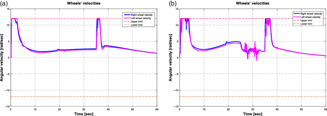
Since in practice the velocity of motors is limited, velocity constraints are considered. Figures 10-a and 10-b indicate the angular velocities of the right and left wheels for the first robot using LMPC and NMPC, respectively. It is worth mentioning that the constraints are applied for all three robots and both controllers. It is seen that the constraints are satisfied, and the velocities cannot exceed the limits defined as desirable when using the two control methods.

Fig. 10.

Angular velocities for robot 1 (a) LMPC. (b) NMPC.

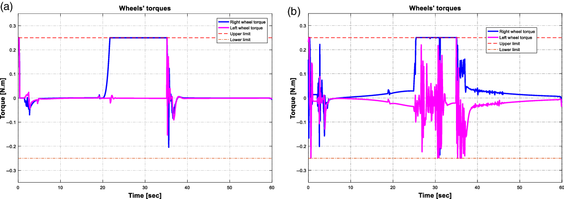
Moreover, the torques of motors are limited in practice as well. Figures 11-a and 11-b show the constrained torques for the first robot using the two control methods LMPC and NMPC, respectively. The constraints are applied to all three robots and for both cases without and with formation control. It is seen that constraints on the control variables are satisfied. In addition, the control goals can be achieved when the input signals are constrained.

Fig. 11.

Wheels’ torques for robot1 (a) LMPC. (b) NMPC.

Case study 2: different types of formation

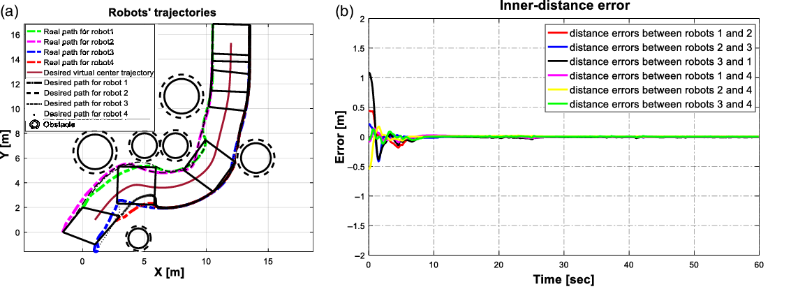
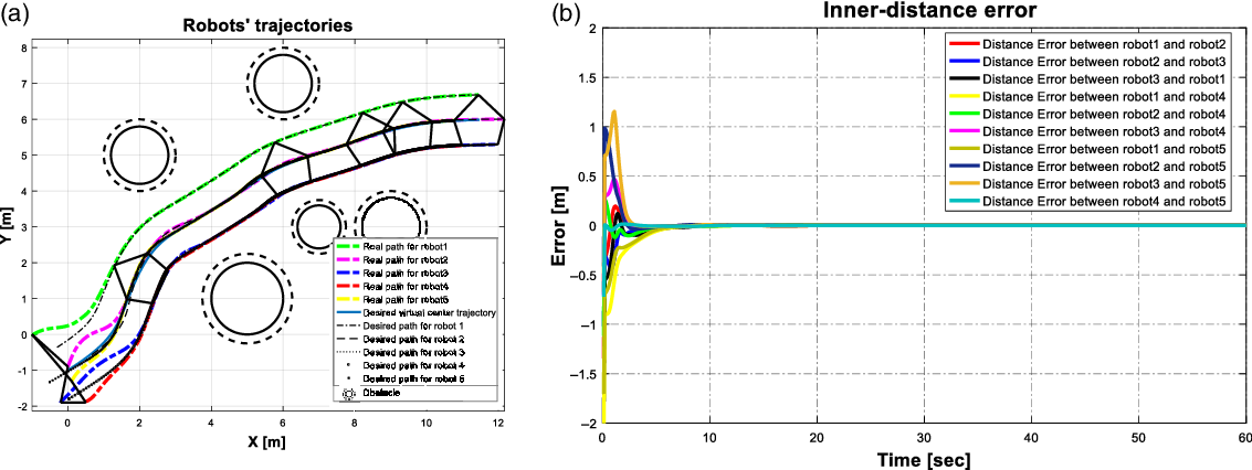
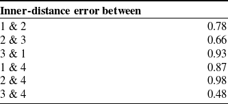
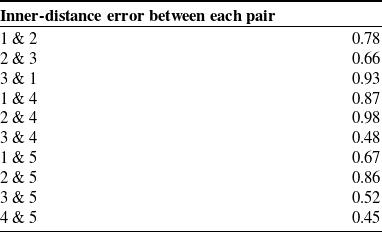
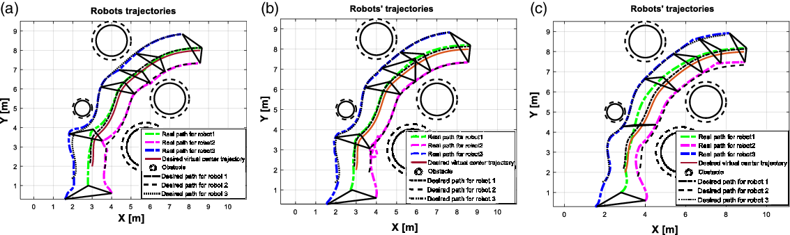
The simulation is run for many different trajectories and different formation geometries in the presence of obstacles. Figures 12-a, 12-b, and 12-c show the simulation results for a system consisting of four agents which navigate in an environment containing six obstacles in different radii where the proposed NMPC method is applied to the system. Another example can be seen in Figs. 13-a, 13-b, and 13-c where LMPC is applied to a five-agent system moving to its goal through five obstacles. The results show that the proposed control algorithm can be applied to a larger number of WMRs with different formation shapes in the presence of more obstacles. The two criteria mentioned in section 5 are shown in Figs. 12-b, 12-c, 13-b, and 13-c. Furthermore, the integrated time absolute error for both cases is reported in Tables VIII, IX, X, and XI. It is worth mentioning that the order error becomes zero for all robots after a short time for both cases.

Fig. 12.

NMPC case study 2. (a) VC and robots’ trajectories. (b) The inner-distance error between the robot.

Fig. 13.

LMPC case study 2. (a) VC and robots’ trajectories. (b) The inner-distance error between the robots.

Table VIII.

Integrated time absolute error of x, y, and angle, case study 2–1.

Table IX.

Integrated time absolute inner-distance error, case study 2–1.

Table X.

Integrated time absolute error of x, y, and angle, case study 2–2.

Table XI.

Integrated time absolute inner-distance error, case study 2–2.

Case study 3: the performance of the controllers in the case of applying time-varying disturbance during the whole simulation period

In this section, the performance of the proposed methods in the presence of harmonic disturbance is discussed. In addition, a comparison between Feed-Back Linearization (FBL) used in [Reference Abbaspour, Moosavian and Alipour20] and our new control methods is presented. There are many advantages of using the NMPC method over feedback linearization. NMPC uses the feedback of nonlinear systems to find the optimal control signals by predicting and optimizing the future behavior of the system. This leads to a system that is robust to the disturbance caused by the imperfect motors and sensors. In addition, the NMPC control system can operate with limits on control variables, state variables, and output variables. One of the drawbacks of feedback linearization is the lack of robustness to disturbances and uncertainties. Moreover, the control variables, state variables, and output variables cannot be constrained using FBL.

In this case study, NMPC and LMPC methods are simulated and compared to the control method presented in [Reference Abbaspour, Moosavian and Alipour20]. The system consists of three nonholonomic differential drive WMRs. The three robots are the same as in the first case study, see Table I.

However, a new reference trajectory of the VC is generated using the proposed APF functions. The initial position and orientation of the VC are ${\textbf{x}_{vc}}({t_0}) = {\left[ {\begin{array}{*{20}{c}}0\quad {}{ -3}\quad {}0\end{array}} \right]^T}$ , and the goal pose for the VC to reach is ${\textbf{x}_{vc}}({t=60}) = {\left[ {\begin{array}{*{20}{c}}{3.3}\quad {}{5.8}\quad {}{0.83}\end{array}} \right]^T}$ . The APF parameters are $K = \;0.015,\;\eta = 5.4,\;\zeta = 5.52$ .

Suppose that the initial conditions of the robots are the desired ones. The desired trajectory of each robot is calculated using Eq. 18, where the formation parameters ${x_i},{y_i}$ are given as follows

\begin{align*}{x_1} = 0.104,\quad \, \, \, \, \, {y_1} = 0.136\end{align*}

\begin{align*}{x_2} = - 0.445,\, \, \, \, \, {y_2} = - 0.41\end{align*}

\begin{align*}{x_3} = - 0.88,\, \, \, \, \, {y_3} = 0.88\end{align*}

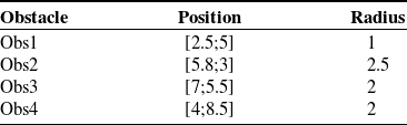
The robots navigate from the initial positions to the goals through 3 obstacles. The position and radius for each obstacle can be found in Table XII.

It is worth noting that constraints were designed for both input and state variables, in the case of LMPC and NMPC. The same constraints on torques and velocities in Table III are used here. As for the FBL, we saturated the control signal so that it does not exceed the torques limits. However, the velocities cannot be constrained using the latter method.

To illustrate the robustness of the proposed control system against continuous harmonic disturbance and compare its performance with that of the control system in [Reference Abbaspour, Moosavian and Alipour20], a time-variant disturbance is added to the first robot for the whole simulation time. This is done by adding a disturbance sinusoidal term to the first robot wheels torques as $\left[ {{\tau _{{1_{d,right}}}};\;{\tau _{{1_{d,left}}}}} \right] = \left[ {0.05\,{\textrm{sin}}(3t);\,0.05\,{\textrm{cos}}\left( {3t} \right)} \right]$ , where ${\tau _{{1_{d,right}}}}$ is the disturbing right wheel torque and ${\tau _{{1_{d,left}}}}$ is the disturbing left wheel torque of the first robot.

The simulation time is 60 s, and the sampling time is ${T_s} = 0.1 \,{\rm{s}}$ . The gains are chosen in the same range so that the comparison between the controllers is fair. The controllers’ parameters are as follows

• NMPC

  \begin{align*}{{{\textbf{Q}}}_N} = {\textrm{diag}}\left( {\left[\! {\begin{array}{*{20}{c}}{20}\quad {}{\begin{array}{*{20}{c}}{24}\quad {}8\quad {}{\begin{array}{*{20}{c}}{0.1}\quad {}{0.1}\end{array}}\end{array}}\end{array}}\!\! \right]} \right),{{{\textbf{R}}}_N} = {\textrm{diag}}\left( {\left[\! {\begin{array}{*{20}{c}}1\quad {}1\end{array}}\! \right]} \right),{N_p} = 10\end{align*}
  \begin{align*}{{{\textbf{P}}}_N} = {\textrm{diag}}\left( {\left[\! {\begin{array}{*{20}{c}}{14}\quad {}{\begin{array}{*{20}{c}}{21}\quad {}{5.6}\quad {}{\begin{array}{*{20}{c}}{0.008}\quad {}{0.008}\end{array}}\end{array}}\end{array}}\!\! \right]} \right),{{{\textbf{L}}}_N} = {\textrm{diag}}\left( {\left[\! {\begin{array}{*{20}{c}}{25}\quad {}{\begin{array}{*{20}{c}}{25}\quad {}{0.5}\quad {}{\begin{array}{*{20}{c}}{0.05}\quad {}{0.05}\end{array}}\end{array}}\end{array}}\!\! \right]} \right)\end{align*}

• MPC

  \begin{align*}{{\textbf{Q}}} = {\textrm{diag}}\left( {\left[\! {\begin{array}{*{20}{c}}{32}\quad {}{\begin{array}{*{20}{c}}{36}\quad {}{10}\quad {}{\begin{array}{*{20}{c}}{0.025}\quad {}{0.025}\end{array}}\end{array}}\end{array}}\!\! \right]} \right),\;\;{{\textbf{R}}} = {\textrm{diag}}\left( {\left[ \!{\begin{array}{*{20}{c}}1\quad {}1\end{array}} \!\right]} \right),{N_p} = 10\end{align*}
  \begin{align*}{{\textbf{P}}} = {\textrm{diag}}\left( {\left[\! {\begin{array}{*{20}{c}}{12}\quad {}{\begin{array}{*{20}{c}}{16}\quad {}4\quad {}{\begin{array}{*{20}{c}}{0.005}\quad {}{0.005}\end{array}}\end{array}}\end{array}}\!\! \right]} \right)\end{align*}

• FBL

  \begin{align*}{{{\textbf{K}}}_p} = {\textrm{diag}}\left( {\left[\! {\begin{array}{*{20}{c}}{24}\quad {}{\begin{array}{*{20}{c}}{28}\quad {}{12}\end{array}}\end{array}}\!\! \right]} \right),{{{\textbf{K}}}_v} = {\textrm{diag}}\left( {\left[\! {\begin{array}{*{20}{c}}{6.5}\quad {}{\begin{array}{*{20}{c}}{6.5}\quad {}7\end{array}}\end{array}}\!\! \right]} \right)\end{align*}
  \begin{align*}{K_K} = 0.015,{K_D} = 16.2,{K_S} = 21.6\end{align*}

Figures 14, 15, and 16 show the simulation result of NMPC, LMPC, and FBL, respectively. Figures 14-b, 15-b, and 16-b illustrate the distance errors between the robots using the three controllers. The order error is zero for all robots during the whole simulation time. The wheels’ velocities of the first robot are shown in Figs. 14-g, 15-g, and 16-g.

Fig. 14.

NMPC case study 3. (a) VC and robots’ trajectories. (b) The inner-distance error between the robots. (c) Errors of robot 1. (d) Errors of robot 2. (e) Errors of robot 3. (f) Wheels’ velocities for the first robot.

Fig. 15.

LMPC case study 3. (a) VC and robots’ trajectories. (b) The inner-distance error between the robots. (c) Errors of robot 1. (d) Errors of robot 2. (e) Errors of robot 3. (f) Wheels’ velocities for the first robot.

Fig. 16.

FBL case study 3. (a) VC and robots’ trajectories. (b) The inner-distance error between the robots. (c) Errors of robot 1. (d) Errors of robot 2. (e) Errors of robot 3. (f) Wheels’ velocities for the first robot.

It is seen that the NMPC can maintain the formation shape in the presence of harmonic and continuous disturbance. The maximum distance error between the robots, in this case, is less than 0.004 m. The errors of the robots are relatively small and oscillate around zero. As for the MPC, the errors are small and oscillate around zero as well.

On the other hand, the inner-distance error of the FBL method is larger and it is seen that there are large initial errors in the first 10 s of the simulation even though the robots start from initial conditions equal to the desired conditions at $t = 0$ . In addition, Fig. 15-c shows the errors of the first robot that have incrementally increased during the simulation time and start to drift from zero after 30 s of the simulation. As a result, the distance errors between robots will be increasing as well. Therefore, the system may not be stable and the formation cannot be kept which can be seen clearly in Fig. 18-c.

As for the velocities, MPC methods can constrain the velocities so that they do not exceed the upper and lower limits. Nevertheless, the FBL method proposed in [Reference Abbaspour, Moosavian and Alipour20] cannot do that which leads to high velocities values that cannot be achieved practically because the wheels’ velocities are limited in practice.

The performance of the three controllers is also compared using the criteria in Tables XIII and XIV. From Table XIII, the errors of our proposed controllers are less by far than the controller proposed in [Reference Abbaspour, Moosavian and Alipour20]. As for the integrated time absolute inner-distance error which is reported in Table XIV, the distance errors of the NMPC and LMPC are significantly less than the FBL approach.

Given the above arguments, it can be concluded that both LMPC methods show a higher degree of robustness against time-variant and long-time disturbance than the FBL. Large initial errors are observed in the case of FBL when the system starts from initial conditions that are identical to the reference path. Therefore, it is better to start from initial conditions that are near enough, but not identical, to the reference trajectory, in the case of FBL.

Case study 4: comparison between our proposed controllers and Laguerre MPC

In this section, a comparison between Laguerre MPC [Reference Ettefagh, Naraghi, Towhidkhah and Izi27] and our new control methods is presented. Laguerre MPC method is applied to the linearized dynamic system unlike paper [Reference Ettefagh, Naraghi, Towhidkhah and Izi27] where the controller is applied to the linearized kinematic system. The main advantage of using Laguerre-based MPC over the traditional MPC is the reduction of computation times [Reference Wang46]. The control signal in the case of traditional MPC may use a very large number of parameters, leading to a heavy computational load. Alternatively, a more relevant approach is by using the Laguerre network in the design of MPC [Reference Wang37]. This will reduce the number of calculations. In fact, the traditional MPC uses a total number of decision variables equals $m \times {N_p}$ where m is the number of inputs and ${N_p}$ is the prediction horizon, while the Laguerre-based MPC captures the control sequence using a smaller number of variables equals to $m \times {N_c}$ where ${N_c}$ is the control horizon which is usually smaller than the predictive horizon ${N_p}$ .

In this case study, NMPC and LMPC methods are simulated and compared with the control method presented in [Reference Ettefagh, Naraghi, Towhidkhah and Izi27]. The system consists of three nonholonomic differential drive WMRs. The parameters of the three robots are the same as in the first case study, see Table I.

However, a new reference trajectory for the VC is generated using the proposed APF functions. The initial position and orientation of the VC are ${{{\textbf{x}}}_{vc}}({t_0}) = {\left[ {\begin{array}{*{20}{c}}3\;\;\;\; {}2\;\;\;\; {}0\end{array}} \right]^T}$ , and the goal point for the VC to reach is ${{{\textbf{x}}}_{vc}}({t=60}) = {\left[ {\begin{array}{*{20}{c}}9\;\;\;\; {}8\;\;\;\; {}0.03\end{array}} \right]^T}$ . The APF parameters are $K = \;0.015,\;\;\eta = 7.2,\;\;\zeta = 3.8$ .

The initial position and orientation of each robot are ${{{\textbf{x}}}_1}({t_0}) = {\left[ {\begin{array}{*{20}{c}}{2.8}\;\;\;\; {}1\;\;\;\; {}{0.368}\end{array}} \right]^T},\;\;{{{\textbf{x}}}_2}({t_0}) = {\left[ {\begin{array}{*{20}{c}}4\;\;\;\; {}{0.6}\;\;\;\; {}{0.098}\end{array}} \right]^T},\;\;{{{\textbf{x}}}_3}({t_0}) = {\left[ {\begin{array}{*{20}{c}}{1.6}\;\;\;\; {}{0.3}\;\;\;\; {}{ -0.195}\end{array}} \right]^T}$ . The desired trajectory of each robot is calculated using Eq. 18, where the formation parameters ${x_i},{y_i}$ are given as follows

\begin{align*}\!\!\!{x_1} = 0.104, \, \, \, \, \, \;\; {y_1} = 0.136\end{align*}

\begin{align*}{x_2} = - 0.012, \, \, \, \, \, {y_2} = - 0.656\end{align*}

\begin{align*}{x_3} = - 0.880, \, \, \, \, \, {y_3} = 0.880\end{align*}

The robots navigate from the initial positions to the goals through 4 obstacles. The position and radius for each obstacle can be found in Table XV.

It is worth noting that constraints were designed for both input and state variables, in the case of LMPC, NMPC, and Laguerre-based MPC. The same constraints on torques and velocities in Table III are used here.

To illustrate the robustness of the proposed control system against disturbance and compare its performance with that of the control system in [Reference Ettefagh, Naraghi, Towhidkhah and Izi27], a disturbance is applied to the first robot in the time interval [Reference Lee and Chwa25, Reference Spong, Hutchinson and Vidyasagar35] s where the total simulation time is 60 s and the sampling time is ${T_s}\; = \;0.1\, {\rm{s}}$ . To this end, the torque of the right wheel is multiplied by 0.7, and the torque of the left wheel is multiplied by 0.01. The performance of the three aforementioned controllers can be seen in Figs. 17–21.

Fig. 17.

Trajectories for the virtual center of the formation and the real path of three robots using(a) NMPC. (b) LMPC. (c) Laguerre MPC.

Fig. 18.

Errors of the first robot using (a) NMPC. (b) LMPC. (c) Laguerre MPC.

Fig. 19.

Errors of the second robot using (a) NMPC. (b) LMPC. (c) Laguerre MPC.

Fig. 20.

Errors of the third robot using (a) NMPC. (b) LMPC. (c) Laguerre MPC.

Fig. 21.

The inner-distance errors between robots using (a) NMPC. (b) LMPC. (c) Laguerre MPC.

The gains are chosen in the same range so that the comparison between the controller performances be fair. The controllers’ parameters are as follow

• NMPC

  \begin{align*}{{{\textbf{Q}}}_N} = {\textrm{diag}}\left( {\left[\! {\begin{array}{*{20}{c}}{20}\quad {}{\begin{array}{*{20}{c}}{24}\quad {}8\quad {}{\begin{array}{*{20}{c}}{0.1}\quad {}{0.1}\end{array}}\end{array}}\end{array}}\!\!\! \right]} \right),\;{\;}{\textbf{R}_N} = {\textrm{diag}}\left( {\left[\! {\begin{array}{*{20}{c}}1\quad {}1\end{array}}\! \right]} \right),\;\;{N_p} = 10\end{align*}
  \begin{align*}{{{\textbf{P}}}_N} = {\textrm{diag}}\left( {\left[\! {\begin{array}{*{20}{c}}{14}\quad {}{\begin{array}{*{20}{c}}{21}\quad {}{5.6}\quad {}{\begin{array}{*{20}{c}}{0.008}\quad {}{0.008}\end{array}}\end{array}}\end{array}}\!\! \right]} \right),\;\;{{{\textbf{L}}}_N} = {\textrm{diag}}\left( {\left[\! {\begin{array}{*{20}{c}}{25}\quad {}{\begin{array}{*{20}{c}}{25}\quad {}{0.5}\quad {}{\begin{array}{*{20}{c}}{0.05}\quad {}{0.05}\end{array}}\end{array}}\end{array}}\!\! \right]} \right)\end{align*}

• LMPC

  \begin{align*}{{\textbf{Q}}} = {\textrm{diag}}\left( {\left[\! {\begin{array}{*{20}{c}}{32}\quad {}{\begin{array}{*{20}{c}}{36}\quad {}{10}\quad {}{\begin{array}{*{20}{c}}{0.025}\quad {}{0.025}\end{array}}\end{array}}\end{array}}\!\! \right]} \right),\;\;{{\textbf{R}}} = {\textrm{diag}}\left( {\left[ \!{\begin{array}{*{20}{c}}1\quad {}1\end{array}}\! \right]} \right),\;\;{N_p} = 10\end{align*}
  \begin{align*}{{\textbf{P}}} = {\textrm{diag}}\left( {\left[\! {\begin{array}{*{20}{c}}{12}\quad {}{\begin{array}{*{20}{c}}{16}\quad {}4\quad {}{\begin{array}{*{20}{c}}{0.005}\quad {}{0.005}\end{array}}\end{array}}\end{array}}\!\!\! \right]} \right)\end{align*}

• Laguerre MPC

  \begin{align*}{{\textbf{Q}}} = {\textrm{diag}}\left( {\left[\! {\begin{array}{*{20}{c}}{52}\quad {}{\begin{array}{*{20}{c}}{67}\quad {}{30}\quad {}{\begin{array}{*{20}{c}}{0.063}\quad {}{0.063}\end{array}}\end{array}}\end{array}}\!\! \right]} \right),\;\;{{\textbf{R}}} = {\textrm{diag}}\left( {\left[\! {\begin{array}{*{20}{c}}1\quad {}1\end{array}}\! \right]} \right),\;\;{N_p} = 10\end{align*}
  \begin{align*}{{\textbf{P}}} = {\textrm{diag}}\left( {\left[\! {\begin{array}{*{20}{c}}{14}\quad {}{\begin{array}{*{20}{c}}{10.8}\quad {}4\quad {}{\begin{array}{*{20}{c}}{0.001}\quad {}{0.001}\end{array}}\end{array}}\end{array}}\!\! \right]} \right),\;\;a = \left[ {0.8;\,0.8} \right],\;\;N = \left[ {3;\,3} \right]\end{align*}

Table XII.

Obstacle specifications.

Table XIII.

Integrated time absolute error of x, y, and angle, case study 3.

Table XIV.

Integrated time absolute inner-distance error, case study 3.

Table XV.

Obstacle specifications.

Table XVI.

Integrated time absolute error of x, y, and angle, case study 4.

Table XVII.

Integrated time absolute inner-distance error, case study 4.

The proposed control strategy is successfully simulated in terms of Laguerre-based MPC. It is seen that the errors of the Laguerre-based MPC are greater than the errors of the other two controllers. Furthermore, the NMPC has the best performance. This is reasonable since the system to be controlled is nonlinear and the initial errors are relatively large. The conventional LMPC and Laguerre-based MPC both are based on the linearized dynamic system; therefore, large initial errors may yield an inaccurate approximation of the system which in turn can lead to a steady-state error which can be seen clearly in the results of both controllers, especially Laguerre-based MPC. However, the LMPC steady-state error is significantly small.

The performance of the three controllers is also compared using the criteria in Tables XVI and XVII. From Table XVI, the errors of our proposed controllers are less by far than the controller proposed in [Reference Ettefagh, Naraghi, Towhidkhah and Izi27]. As for the integrated time absolute inner-distance error which is reported in Table XVII, the inner-distance error of the NMPC is significantly less than the other two approaches.