1 Introduction
Self-sustained oscillations occur due to hydrodynamic instabilities observed in the wakes behind bluff bodies (Provansal, Mathis & Boyer Reference Provansal, Mathis and Boyer1987; Monkewitz Reference Monkewitz1988; Emerson et al. Reference Emerson, O’Connor, Juniper and Lieuwen2012), and in the flow field of low density jets (Huerre & Monkewitz Reference Huerre and Monkewitz1985; Li & Juniper Reference Li and Juniper2013a ) and are also due to thermoacoustic interactions in confined reacting flows (Crocco & Cheng Reference Crocco and Cheng1956; Oyediran, Darling & Radhakrishnan Reference Oyediran, Darling and Radhakrishnan1995; Lieuwen & Yang Reference Lieuwen and Yang2005). Systems having temporally unstable global modes behave as oscillators (Huerre & Monkewitz Reference Huerre and Monkewitz1990). Harmonic excitation of such unstable mean flows essentially modulates the generation of large-scale coherent structures, thereby enhancing the transport of momentum across the flow (Greenblatt & Wygnanski Reference Greenblatt and Wygnanski2000). Therefore, efficient mixing through high momentum transfer and control of intrinsic global modes can be achieved through a rigorous understanding of the interaction between the external excitation and the intrinsic oscillatory modes observed in fluid mechanical systems. In the present study, we investigate this interaction in a thermoacoustically unstable system where an external harmonic forcing is used to suppress unwanted self-sustained periodic oscillations.
Thermoacoustic instability has hampered the development of practical combustion systems such as gas turbine engines, rocket motors and industrial burners (Juniper & Sujith Reference Juniper and Sujith2018). Such an instability refers to the occurrence of large amplitude pressure oscillations in a combustion chamber. These instabilities occur primarily due to a closed loop interaction between the acoustic waves (
 $p^{\prime }$
) inside the combustor and the unsteady heat release rate (
 $\dot{q}^{\prime }$
) from the flame. Large levels of vibration caused due to thermoacoustic instability can lead to catastrophic consequences such as structural damage or reduction in the lifetime of combustors (Sujith, Juniper & Schmid Reference Sujith, Juniper and Schmid2016). Therefore, there is a need to either control such instabilities or to suppress them completely.
Various methods have been devised over the years to control these instabilities and thereby increase the operational range of the engines (Dowling & Morgans Reference Dowling and Morgans2005). The control strategies used in the past to suppress thermoacoustic instabilities are of different kinds. Open-loop control strategies, which were able to reduce the thermoacoustic coupling between the acoustic field and the unsteady heat release rate, include perturbing either the shear layers in the flow field (McManus, Vandsburger & Bowman Reference McManus, Vandsburger and Bowman1990) or the acoustic field of the combustor (Najm & Ghoniem Reference Najm and Ghoniem1991). Closed-loop control has also been implemented in a Rijke tube (Dines Reference Dines1984; Heckl Reference Heckl1988), ducted premixed flame (Lang, Poinsot & Candel Reference Lang, Poinsot and Candel1987b ) and in a turbulent diffusion flame (Lang et al. Reference Lang, Poinsot, Bourienne, Candel and Esposito1987a ) to suppress the amplitude of acoustic pressure oscillations through the mechanism of negative feedback between the self-excited sound waves, and the imposed sound waves (external acoustic perturbations). Note that in open-loop control, forcing is applied at different frequencies other than the natural frequency, whereas, in closed-loop control, the feedback signal is applied at the natural frequency, but is phase shifted (Lubarsky et al. Reference Lubarsky, Shcherbik, Zinn, McManus, Fric and Srinivasan2003).
1.1 Forcing on self-sustained oscillatory systems including reacting flow systems
Harmonic forcing has also found its application in self-sustained oscillatory systems. Lubarsky et al. (Reference Lubarsky, Shcherbik, Zinn, McManus, Fric and Srinivasan2003) experimentally studied the effect of fuel flow modulation at a non-resonant frequency on the self-excited thermoacoustic oscillations in a swirl-stabilized combustor. Bellows, Neumeier & Lieuwen (Reference Bellows, Neumeier and Lieuwen2006) studied the nonlinear response of the heat release rate fluctuations to flow perturbations in the context of a swirling premixed flame. The response in the heat release rate oscillation was shown to saturate at a sufficiently high amplitude of forcing. In a different study, Bellows, Hreiz & Lieuwen (Reference Bellows, Hreiz and Lieuwen2008) reported the effectiveness of forcing for controlling the self-excited thermoacoustic oscillations. However, they observed a reduction in amplitude only for a few selected forcing frequencies. Therefore, a systematic investigation of forced response for a wide range of forcing frequency and amplitude is desirable in a thermoacoustic system to qualitatively identify the regime of amplitude reduction in terms of the forcing parameters. Further, characterizing the dynamical states and mechanisms of amplitude reduction in the context of dynamical systems theory is essential for a better understanding of the phenomenon. In a recent study by Kashinath, Li & Juniper (Reference Kashinath, Li and Juniper2018), forced synchronization leading to periodic, quasi-periodic and chaotic states is investigated quite elaborately using a simple model of a ducted laminar flame; however, experimental realization of this study is still limited.
Further, upon the application of harmonic excitation on hydrodynamically self-excited flames, different kinds of dynamics and bifurcations have been observed (Li & Juniper Reference Li and Juniper2013b ) before an eventual phase locking between the forcing signal and the natural oscillations of the system. In the recent past, the effect of external acoustic forcing has been investigated elaborately in self-excited jets (Li & Juniper Reference Li and Juniper2013a ,Reference Li and Juniper c ) and self-excited flames (Li & Juniper Reference Li and Juniper2013b ). They have reported different dynamical states including quasiperiodicity (Li & Juniper Reference Li and Juniper2013a ,Reference Li and Juniper b ) as well as different synchronization states including phase slipping and phase trapping (Li & Juniper Reference Li and Juniper2013c ). Further, Hochgreb and her co-workers (Kim & Hochgreb Reference Kim and Hochgreb2011, Reference Kim and Hochgreb2012; Balusamy et al. Reference Balusamy, Li, Han, Juniper and Hochgreb2015; Han, Balusamy & Hochgreb Reference Han, Balusamy and Hochgreb2015; Han & Hochgreb Reference Han and Hochgreb2015; Balusamy et al. Reference Balusamy, Li, Han and Hochgreb2017) have extensively studied the dynamics and the response of stratified lean-premixed flames subjected to external acoustic velocity perturbations. Most of their studies (Kim & Hochgreb Reference Kim and Hochgreb2011, Reference Kim and Hochgreb2012; Han et al. Reference Han, Balusamy and Hochgreb2015; Han & Hochgreb Reference Han and Hochgreb2015; Balusamy et al. Reference Balusamy, Li, Han and Hochgreb2017) were focussed on investigating the forced flame response by estimating the flame transfer/describing functions (FTF/FDF). Balusamy et al. (Reference Balusamy, Li, Han, Juniper and Hochgreb2015), however, characterized the forced dynamics of a self-excited thermoacoustic system using the framework of forced synchronization. They reported the observations of pulling or pushing of the response frequency associated with the self-excited mode towards or away from the forcing frequency for different conditions of harmonic forcing.
Yoshida et al. (Reference Yoshida, Yazaki, Ueda and Biwa2013) investigated forced synchronization phenomena in a thermoacoustic engine, wherein the pressure oscillations are amplified and sustained due to the temperature gradient between heat exchangers and not due to the unsteady heat release rate from the flame. They have evidenced the reduction in amplitude associated with the natural dynamics for a selected value of frequency detuning. Although some progress has been made in understanding the response dynamics of forced limit cycle oscillations of thermoacoustic systems, the reduction in the overall response amplitude (amplitude of the forced system) due to forcing needs more rigorous investigation.
In the present study, we experimentally and theoretically investigate the effect of forcing on the self-excited periodic oscillations developed in a thermoacoustic system, the horizontal Rijke tube. We further show a qualitative similarity of the forced dynamics observed in the experiments with a reduced-order model developed for the system. One of the objectives is to obtain a complete picture in terms of response dynamics as well as synchronization behaviour of the forced thermoacoustic system.
1.2 Forced synchronization and amplitude quenching
The phenomenon of forced synchronization (synchronization of unidirectionally coupled periodic oscillators) has been gaining increased attention and has been extensively studied both theoretically (Pikovsky, Rosenblum & Kurths Reference Pikovsky, Rosenblum and Kurths2003; Balanov et al. Reference Balanov, Janson, Postnov and Sosnovtseva2009) and experimentally (Kiss & Hudson Reference Kiss and Hudson2001; Boccaletti et al. Reference Boccaletti, Allaria, Meucci and Arecchi2002; Battogtokh, Aihara & Tyson Reference Battogtokh, Aihara and Tyson2006). The forced response of a system depends on the values of the frequency and the amplitude of forcing. Such response dynamics of a forced system can be effectively represented by a synchronization region in the parametric space of forcing amplitude and frequency, known as the Arnold tongue (Balanov et al. Reference Balanov, Janson, Postnov and Sosnovtseva2009). Most of the theoretical studies on forced synchronization are based on van der Pol oscillators, which mimic a variety of oscillatory phenomena in electric circuits (van der Pol Reference van der Pol1920), electrocardiograms (Van Der Pol & Van Der Mark Reference Van Der Pol and Van Der Mark1928), semiconductor lasers (Blažek Reference Blažek1968), neuronal activity (Nomura et al. Reference Nomura, Sato, Doi, Segundo and Stiber1993), etc. Further, the phenomenon of forced synchronization has been experimentally implemented to control or suppress chaos (Anishchenko et al. Reference Anishchenko, Vadivasova, Postnov and Safonova1992; Kiss & Hudson Reference Kiss and Hudson2001), and also to suppress oscillatory instability (Keen & Fletcher Reference Keen and Fletcher1969). Using a simple experimental set-up consisting of an organ pipe and a loudspeaker, Abel, Ahnert & Bergweiler (Reference Abel, Ahnert and Bergweiler2009) gave an experimental evidence of forced synchronization in acoustics.
Forced synchronization of periodic oscillations is usually achieved through the routes of phase locking and suppression (Balanov et al.
Reference Balanov, Janson, Postnov and Sosnovtseva2009). Upon increasing the forcing amplitude, when the frequency difference between the forcing and the natural oscillation of a given system is very small, the frequency of forced oscillations, also called the main frequency in other literature (Balanov et al.
Reference Balanov, Janson, Postnov and Sosnovtseva2009), shifts gradually towards the forcing frequency (
 $f_{f}$
) and, finally, coincides with
 $f_{f}$
; the mechanism is known as phase locking. Hereafter, we call the frequency of forced oscillation the response frequency (
 $f_{r}$
). On the other hand, suppression of the self-sustained oscillations occurs for a relatively larger value of the frequency difference, wherein the amplitude of natural oscillations is suppressed without exhibiting any shift in frequency, as the forcing amplitude is increased. The route of phase locking is attained through a saddle-node bifurcation, whereas, the suppression route is reached through a torus-death bifurcation (Balanov et al.
Reference Balanov, Janson, Postnov and Sosnovtseva2009; Hyodo & Biwa Reference Hyodo and Biwa2018).
Suppression is further classified as synchronous quenching (Odajima, Nishida & Hatta Reference Odajima, Nishida and Hatta1974; Ohsawa Reference Ohsawa1980) and asynchronous quenching (Minorsky Reference Minorsky1967) depending upon the value of frequency detuning between the forcing and the natural oscillation. When the frequency detuning is relatively small, the suppression of self-sustained oscillation is known as synchronous quenching. However, synchronous quenching of natural oscillation is associated with resonance amplification of the forcing signal, in which the overall response amplitude of the forced system increases to a higher value in the synchronization region. On the other hand, when frequency detuning is relatively large, the suppression of self-sustained oscillation is known as asynchronous quenching (Minorsky Reference Minorsky1967) where the resonant amplification of the forcing signal does not occur. Such a type of suppression is caused by an asymptotic loss of stability of self-excited oscillations due to the disturbance induced by the imposed forcing and leads to a reduction in the overall amplitude of the forced system (Keen & Fletcher Reference Keen and Fletcher1969).
Therefore, studying the applicability of asynchronous quenching is important to mitigate the amplitude of undesired acoustic oscillations observed in practical combustors. Such a type of suppression phenomenon was experimentally evidenced in the control of ion-sound instability (Keen & Fletcher Reference Keen and Fletcher1969), in self-excited ionization waves (Ohe & Takeda Reference Ohe and Takeda1974) and even in the control of thermoacoustic instability (Guan et al. Reference Guan, Gupta, Kashinath and Li2018). Further, the reduction in response amplitude of thermoacoustic oscillation forced at non-resonant frequencies has been reported in previous studies (Lubarsky et al. Reference Lubarsky, Shcherbik, Zinn, McManus, Fric and Srinivasan2003; Bellows et al. Reference Bellows, Hreiz and Lieuwen2008; Guan et al. Reference Guan, Gupta, Kashinath and Li2018; Kashinath et al. Reference Kashinath, Li and Juniper2018). However, they did not focus on explaining the mechanism behind such a quenching of natural oscillations due to forcing. In the present study, we apply the knowledge of forced synchronization and the associated quenching phenomena in studying systematically the forced response of limit cycle oscillations of a horizontal Rijke tube.
We employ external harmonic forcing through a system of acoustic drivers when the system dynamics exhibits self-sustained limit cycle oscillations at the fundamental longitudinal mode of the duct. By varying the amplitude and frequency (across the natural frequency) of forcing, we report an experimental observation of synchronous quenching of self-sustained oscillation and resonant amplification of the forcing in the synchronization region of the Arnold tongue along with the exhibition of different states during the process of forced synchronization. We, further, report an experimental observation of a significant reduction in root-mean-square (r.m.s.) amplitude of natural oscillations (by 80 % of the unforced value) when the system is forced with a frequency far lower than the natural frequency (in the present case, it happens to be close to a subharmonic frequency). We also observe qualitatively similar dynamics in a theoretical model developed for the horizontal Rijke tube (Balasubramanian & Sujith Reference Balasubramanian and Sujith2008). By varying the forcing amplitude and the forcing frequency, we explore the phenomena of synchronous and asynchronous quenching in the model. We further try to explore the effect of harmonic forcing on the thermoacoustic coupling between the acoustic pressure (
 $p^{\prime }$
) and the heat release rate (
 $\dot{q}^{\prime }$
) oscillations obtained from the model. The phenomenon of asynchronous quenching is found to be associated with a shift in phase difference between
 $p^{\prime }$
and
 $\dot{q}^{\prime }$
from zero (during phase synchronization) to
 $\unicode[STIX]{x03C0}/2$
.
2 Experimental set-up
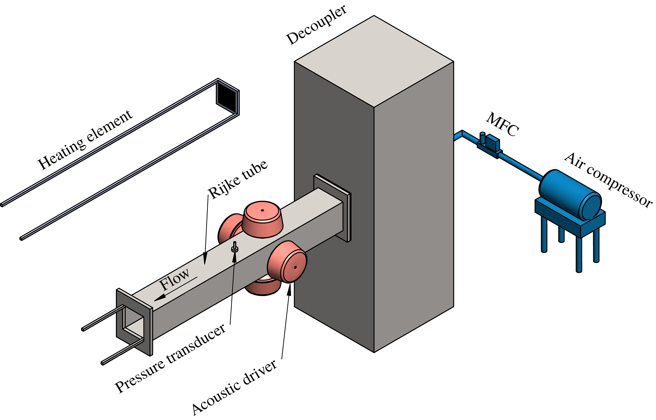
We perform experiments on a horizontal Rijke tube (schematic shown in figure 1), which is 1 m long with a square cross-section (9.2 cm × 9.2 cm). An electrically heated wire mesh acts as a compact heat source which is powered by an external DC power supply. The mean flow of air is provided by means of a compressor and is maintained constant at 100 slpm using a mass flow controller (Alicat Scientific, MCR series, with an uncertainty of
 $\pm$
(0.8 % of the reading + 0.2 % of full scale) and the range of 0–500 slpm). The air is passed through a rectangular chamber (120 cm × 45 cm × 45 cm), referred to as a decoupler, to eliminate the upstream fluctuations (hydrodynamic and acoustic) and to make the inlet flow steady. Therefore, pressure fluctuations at both ends of the Rijke tube become negligible. A detailed description of the set-up can be found in Gopalakrishnan & Sujith (Reference Gopalakrishnan and Sujith2015).
Schematic of a horizontal Rijke tube set-up used in the present study.

The location of the heater inside the duct is held constant throughout the study at 27 cm from the end connected to the decoupler. Four wall mounted acoustic drivers (loud speaker, Ahuja AU60, at a distance of 62.5 cm from the inlet) along with an amplifier are used to provide harmonic forcing signal in the system. Note that the forcing amplitude of the loudspeaker is expressed in its input unit, i.e. mV, throughout the paper and not converted into physical units such as that of acoustic velocity (
 $\text{m}~\text{s}^{-1}$
) or pressure amplitude (Pa). Such conversions can be done through several means (Li & Juniper Reference Li and Juniper2013a
; Balusamy et al.
Reference Balusamy, Li, Han, Juniper and Hochgreb2015). We retain the mV readings, considering the fact that such peak-to-peak voltage is directly proportional to the amplitude of acoustic pressure (Li & Juniper Reference Li and Juniper2013a
).
A piezoelectric transducer (PCB 103B02, sensitivity
 $217.5~\text{mV}~\text{kPa}^{-1}$
and uncertainty
 $\pm 0.15$
Pa) mounted at the wall, close to the midpoint along the length of the duct, is used to measure the acoustic pressure fluctuations in the system. The system is preheated for 10 min by supplying a constant voltage of 3.5 V to the heater to ensure that the temperature is steady in the vicinity of the heater. The subcritical Hopf bifurcation takes place at a heater power value of 1.21 kW (uncertainty
 $\pm 0.4$
W). For the forcing study, the power supplied to the heater is maintained constant at 1.24 kW throughout the experiments. Data are acquired at a sampling frequency of 10 kHz. The bin size (frequency resolution) of the fast Fourier transform of the measured signal is 0.3 Hz. To ensure consistent ambient conditions, we maintain an initial temperature at
 $23\pm 3\,^{\circ }\text{C}$
and a relative humidity at 55 % for each experiment. We also determine the exponential decay rate of the system by giving an acoustic pulse in the absence of the flow (Mariappan Reference Mariappan2012). To ensure repeatability, the experiments are conducted only when the decay rate lies within
 $\pm 10\,\%$
of the mean value, found to be
 $19.0~\text{s}^{-1}$
.
3 Model
We use a reduced-order model for the horizontal Rijke tube developed by Balasubramanian & Sujith (Reference Balasubramanian and Sujith2008). The model for a one-dimensional acoustic field is derived from the linearized momentum (3.1) and energy (3.2) equations for a medium with a perfect, inviscid and non-heat-conducting gas, neglecting the effects of mean flow (zero Mach number approximation, Nicoud & Wieczorek Reference Nicoud and Wieczorek2009) and mean temperature gradient:
 $$\begin{eqnarray}\displaystyle & \displaystyle \bar{\unicode[STIX]{x1D70C}}\frac{\unicode[STIX]{x2202}\tilde{u} ^{\prime }}{\unicode[STIX]{x2202}\tilde{t}}+\frac{\unicode[STIX]{x2202}\tilde{p}^{\prime }}{\unicode[STIX]{x2202}\tilde{x}}=0, & \displaystyle\end{eqnarray}$$
 $$\begin{eqnarray}\displaystyle & \displaystyle \frac{\unicode[STIX]{x2202}\tilde{p}^{\prime }}{\unicode[STIX]{x2202}\tilde{t}}+\unicode[STIX]{x1D6FE}\bar{p}\frac{\unicode[STIX]{x2202}\tilde{u} ^{\prime }}{\unicode[STIX]{x2202}\tilde{x}}=(\unicode[STIX]{x1D6FE}-1)\dot{\tilde{Q}}^{\prime }\unicode[STIX]{x1D6FF}(\tilde{x}-\tilde{x}_{f}), & \displaystyle\end{eqnarray}$$
where
 $\unicode[STIX]{x1D70C}$
and
 $\unicode[STIX]{x1D6FE}$
are the density and the ratio of specific heats of the medium. The heat release rate (
 $\dot{\tilde{Q}}^{\prime }$
) in the duct is modelled using a modified form of King’s law (King Reference King1914) given by Heckl (Reference Heckl1990). The variables are non-dimensionalized and the resulting set of partial differential equations is then reduced to a set of ordinary differential equations (ODE) using the Galerkin technique (Lores & Zinn Reference Lores and Zinn1973). To that end, the non-dimensional velocity (
 $u^{\prime }$
) and the non-dimensional pressure (
 $p^{\prime }$
) fluctuations in the duct are written in terms of basis functions or the Galerkin modes (Balasubramanian & Sujith Reference Balasubramanian and Sujith2008). These basis functions are essentially the natural acoustic modes of the duct in the absence of heat release. These functions further satisfy the boundary conditions [
 $p^{\prime }(0,t)=0$
;
 $p^{\prime }(1,t)=0$
] and can be written as follows:
 $$\begin{eqnarray}\displaystyle & \displaystyle u^{\prime }(x,t)=\mathop{\sum }_{j=1}^{N}\unicode[STIX]{x1D702}_{j}(t)\cos (j\unicode[STIX]{x03C0}x), & \displaystyle\end{eqnarray}$$
 $$\begin{eqnarray}\displaystyle & \displaystyle p^{\prime }(x,t)=-\mathop{\sum }_{j=1}^{N}\dot{\unicode[STIX]{x1D702}_{j}}(t)\frac{\unicode[STIX]{x1D6FE}M}{j\unicode[STIX]{x03C0}}\sin (j\unicode[STIX]{x03C0}x), & \displaystyle\end{eqnarray}$$
where
 $\unicode[STIX]{x1D702}_{j}$
and
 $\dot{\unicode[STIX]{x1D702}}_{j}$
represent the time varying coefficients of the
 $j$
th mode of the acoustic velocity (
 $u^{\prime }$
) and the acoustic pressure (
 $p^{\prime }$
), respectively, and
 $N$
represents the number of Galerkin modes considered. Here,
 $M$
is the Mach number of the mean flow and
 $\unicode[STIX]{x1D6FE}$
is the ratio of specific heats of air at ambient condition.
The temporal evolution of the system is thus described by the following set of ordinary differential equations:
 $$\begin{eqnarray}\displaystyle & \displaystyle \frac{\text{d}\unicode[STIX]{x1D702}_{j}}{\text{d}t}=\dot{\unicode[STIX]{x1D702}}_{j}, & \displaystyle\end{eqnarray}$$
 $$\begin{eqnarray}\displaystyle & \displaystyle \frac{\text{d}\dot{\unicode[STIX]{x1D702}}_{j}}{\text{d}t}+2\unicode[STIX]{x1D701}_{j}\unicode[STIX]{x1D714}_{j}\dot{\unicode[STIX]{x1D702}}_{j}+{\unicode[STIX]{x1D714}_{j}}^{2}\unicode[STIX]{x1D702}_{j}=-j\unicode[STIX]{x03C0}K\left[\sqrt{\left|\frac{1}{3}+u_{f}^{\prime }(t-\unicode[STIX]{x1D70F})\right|}-\sqrt{\frac{1}{3}}\right]\sin (j\unicode[STIX]{x03C0}x_{f}), & \displaystyle\end{eqnarray}$$
where
 $$\begin{eqnarray}u_{f}^{\prime }(t-\unicode[STIX]{x1D70F})=\mathop{\sum }_{j=1}^{N}\unicode[STIX]{x1D702}_{j}(t-\unicode[STIX]{x1D70F})\cos (j\unicode[STIX]{x03C0}x_{f}).\end{eqnarray}$$
Other parameters are the damping coefficient of the
 $j$
th mode,
 $\unicode[STIX]{x1D701}_{j}$
, non-dimensional angular frequency,
 $\unicode[STIX]{x1D714}$
, non-dimensional heater power,
 $K$
, and non-dimensional velocity,
 $u_{f}^{\prime }$
at the non-dimensional heater location,
 $x_{f}$
. Variables with a tilde are dimensional and those without a tilde are non-dimensional. Here,
 $K$
is analogous to the heater power in experiments and
 $\unicode[STIX]{x1D701}_{j}$
is frequency-dependent damping (Sterling & Zukoski Reference Sterling and Zukoski1991) given by
 $$\begin{eqnarray}\unicode[STIX]{x1D701}_{j}=\frac{1}{2\unicode[STIX]{x03C0}}\left(c_{1}\frac{\unicode[STIX]{x1D714}_{j}}{\unicode[STIX]{x1D714}_{1}}+c_{2}\sqrt{\frac{\unicode[STIX]{x1D714}_{1}}{\unicode[STIX]{x1D714}_{j}}}\right).\end{eqnarray}$$
This model essentially captures the feedback between the heat release rate fluctuations and the acoustic pressure fluctuations. More details of the model can be obtained in Balasubramanian & Sujith (Reference Balasubramanian and Sujith2008). The mathematical model governed by (3.5) and (3.6) represents a nonlinear oscillator which exhibits a transition to the self-sustained oscillatory state through subcritical Hopf bifurcation. This model has been used extensively to study various thermoacoustic phenomena in previous studies (Juniper Reference Juniper2011; Magri & Juniper Reference Magri and Juniper2013; Zhao & Reyhanoglu Reference Zhao and Reyhanoglu2014; Thomas et al. Reference Thomas, Mondal, Pawar and Sujith2018). All the parameters are chosen in such a way that the model exhibits limit cycle oscillations away from the bistable regime.
To study the effect of external perturbations, a harmonic forcing with amplitude,
 $A_{f}$
, and frequency,
 $f_{f}$
, is implemented. Once we include the forcing term, equation (3.6) becomes:
 $$\begin{eqnarray}\frac{\text{d}\dot{\unicode[STIX]{x1D702}}_{j}}{\text{d}t}+2\unicode[STIX]{x1D701}_{j}\unicode[STIX]{x1D714}_{j}\dot{\unicode[STIX]{x1D702}}_{j}+{\unicode[STIX]{x1D714}_{j}}^{2}\unicode[STIX]{x1D702}_{j}=-j\unicode[STIX]{x03C0}K\left[\sqrt{\left|\frac{1}{3}+u_{f}^{\prime }(t-\unicode[STIX]{x1D70F})\right|}-\sqrt{\frac{1}{3}}\right]\sin (j\unicode[STIX]{x03C0}x_{f})+A_{f}\sin (2\unicode[STIX]{x03C0}f_{f}t).\end{eqnarray}$$
For the present study, we vary both
 $A_{f}$
and
 $f_{f}$
independently over a wide range when the system is in the state of limit cycle oscillation and analyse the forced response dynamics of the acoustic pressure (
 $p^{\prime }$
, following (3.4)) in the system. Further, we evaluate heat release rate oscillations (
 $\dot{q}^{\prime }$
, following (3.10)) for different forcing conditions to analyse the normalized and cycle-averaged acoustic power production (
 $\langle p^{\prime }\dot{q}^{\prime }\rangle _{t}$
). The parametric values used for computation are given in table 1.
 $$\begin{eqnarray}\dot{q}^{\prime }=\mathop{\sum }_{j=1}^{N}j\unicode[STIX]{x03C0}K\left[\sqrt{\left|\frac{1}{3}+u_{f}^{\prime }(t-\unicode[STIX]{x1D70F})\right|}-\sqrt{\frac{1}{3}}\right]\sin (j\unicode[STIX]{x03C0}x_{f}).\end{eqnarray}$$
The parametric values used for the computation of Rijke tube model.

4 Results and discussions
During the experiments, we set the heater location (27 cm from the inlet), heater power (1.24 kW corresponding to 4.1 V and 303 A) and the air flow rate (100 slpm) in such a way that the Rijke tube exhibits limit cycle oscillations in acoustic pressure with a natural frequency (
 $f_{n0}$
) of 168.8 Hz (fundamental mode of the system). The dynamics of such a system with the variation of the parameters mentioned above has been well studied by various researchers; see for example, Matveev (Reference Matveev2003), Gopalakrishnan & Sujith (Reference Gopalakrishnan and Sujith2014) and Etikyala & Sujith (Reference Etikyala and Sujith2017). Here, we consider the system in its self-sustained oscillatory state to explore the forced synchronization behaviour when the frequency and the amplitude of forcing are varied independently.
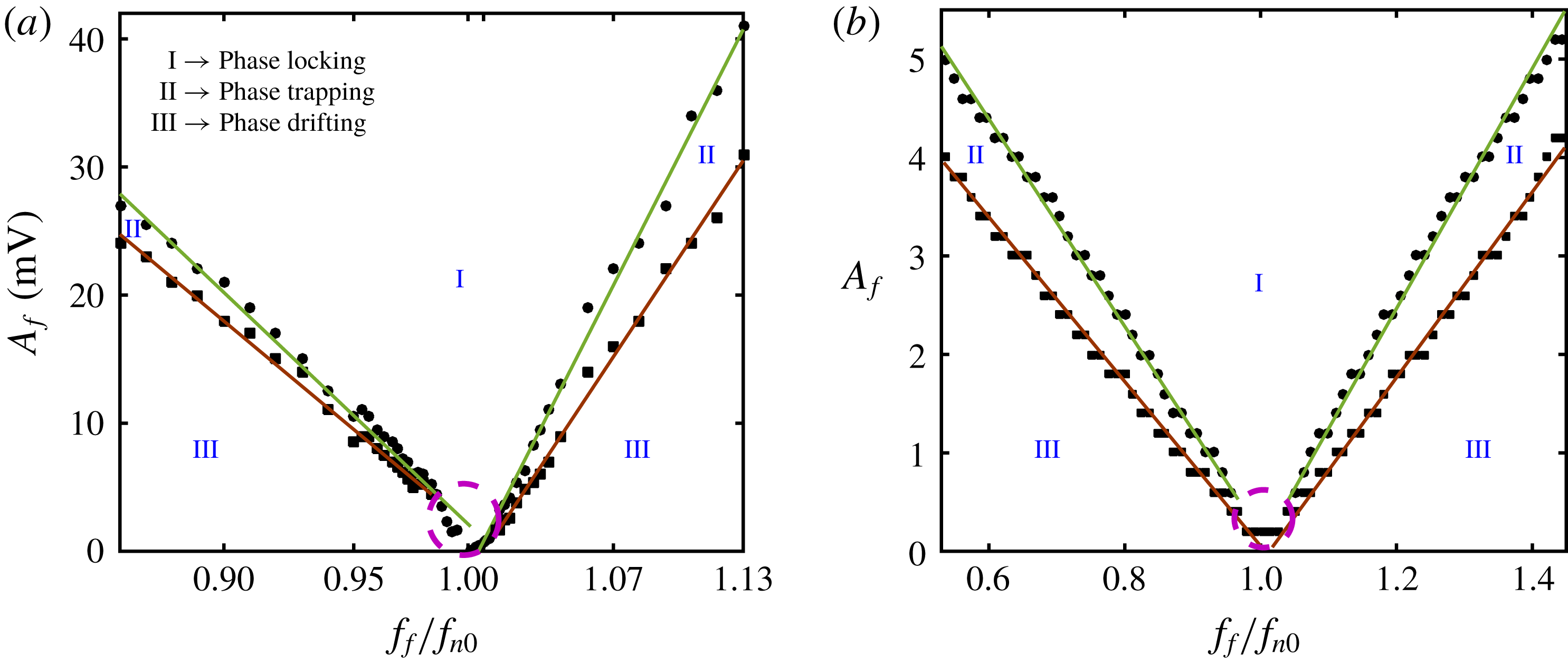
A 1:1 forced synchronization map in the plane of
 $A_{f}$
and
 $f_{f}/f_{n0}$
obtained from (a) the experiment and (b) the model when a harmonic forcing is applied to a self-sustained thermoacoustic oscillator exhibiting limit cycle oscillations. Regions of phase locking, phase trapping and phase drifting are indicated as regions I, II and III, respectively. The synchronization region indicated by phase locking is observed to form an Arnold tongue. Boundaries between regions I and II (●) and between regions II and III (▪) are shown by linearly fitted lines (least squares,
 $R^{2}=0.99\pm 0.0044$
). The regime where phase trapping is not observed is indicated with a dashed circle. Note that the ranges of abscissa and ordinate in (a) and (b) are different, where both plots show a qualitative but not a quantitative comparison between the Arnold tongues obtained from experiment and model.

4.1 Synchronization map
The response dynamics of the acoustic pressure oscillation is presented in the form of 1 : 1 (the ratio between the forcing frequency and the natural frequency at the synchronized state) forced synchronization map (figure 2
a) by varying the forcing amplitude (
 $A_{f}$
) and the normalized forcing frequency (
 $f_{f}/f_{n0}$
) one at a time. Further, the response dynamics obtained from the model is shown in figure 2(b). The different regimes of forced synchronization such as regimes of phase locking, phase trapping and phase drifting (Li & Juniper Reference Li and Juniper2013c
) are identified and illustrated in figures 2(a) and 2(b).
The characterization of the different states of synchronization is based on the dynamics of the instantaneous phase difference (
 $\unicode[STIX]{x0394}\unicode[STIX]{x1D719}$
) between the forcing signal (
 $\unicode[STIX]{x1D719}_{F}$
) with the signal of the forced system (
 $\unicode[STIX]{x1D719}_{p^{\prime }}$
), i.e.
 $\unicode[STIX]{x0394}\unicode[STIX]{x1D719}=|\unicode[STIX]{x1D719}_{F}-\unicode[STIX]{x1D719}_{p^{\prime }}|$
. The instantaneous phases are calculated through Hilbert transform of the respective signals. During the phase-locking state, the instantaneous phases (
 $\unicode[STIX]{x1D719}$
) as well as the frequencies (
 $\unicode[STIX]{x1D714}$
) of the forcing and the response signals show a perfect locking, i.e.
 $|\unicode[STIX]{x0394}\unicode[STIX]{x1D719}|=\text{const.}$
and
 $\unicode[STIX]{x0394}\unicode[STIX]{x1D714}=|\unicode[STIX]{x1D714}_{F}-\unicode[STIX]{x1D714}_{p^{\prime }}|=0$
(Pikovsky et al.
Reference Pikovsky, Rosenblum and Kurths2003). In contrast, during the phase trapping state, the relative phase (
 $\unicode[STIX]{x0394}\unicode[STIX]{x1D719}$
) between the response signal and the forcing signal shows a bounded oscillatory behaviour, which results in the locking of mean frequencies (
 $\unicode[STIX]{x1D714}=\langle \text{d}\unicode[STIX]{x1D719}/\text{d}t\rangle$
) of the signals without exhibiting their instantaneous phase locking (Thévenin et al.
Reference Thévenin, Romanelli, Vallet, Brunel and Erneux2011; Li & Juniper Reference Li and Juniper2013c
). Phase drifting, on the other hand, corresponds to the unbounded growth or decay of the unwrapped relative phase between the forcing and the response signals with time.
With an increase in the forcing amplitude, the region of 1 : 1 synchronization increases, resulting in a V-shaped synchronization region (I, figure 2
a,b), called the Arnold tongue (Pikovsky et al.
Reference Pikovsky, Rosenblum and Kurths2003; Balanov et al.
Reference Balanov, Janson, Postnov and Sosnovtseva2009). The model qualitatively captures the phenomenon of 1 : 1 synchronization (figure 2
b) observed in the experiments (figure 2
a). We notice a region of phase trapping (II, figure 2
a,b) between the regions of phase drifting (III, figure 2
a,b) and phase locking (I, figure 2
a,b) for both
 $f_{f}/f_{n0}<1$
and
 $f_{f}/f_{n0}>1$
.
In the Arnold tongue obtained from experiments (figure 2
a), we observe an asymmetry about
 $f_{n0}$
. The curves are less steep for
 $f_{f}<f_{n0}$
as compared to that observed for
 $f_{f}>f_{n0}$
. Such an asymmetry in the Arnold tongue is due to the nonlinearity involved in the periodic oscillator (Balanov et al.
Reference Balanov, Janson, Postnov and Sosnovtseva2009). A similar asymmetry in the Arnold tongue has been observed in forced low density jets (Hallberg & Strykowski Reference Hallberg and Strykowski2008) and hydrodynamically self-excited jets (Li & Juniper Reference Li and Juniper2013a
,Reference Li and Juniper
c
). However, in another study on a jet diffusion flame, the asymmetry showed the opposite trend, having steeper curves for
 $f_{f}<f_{n0}$
(Li & Juniper Reference Li and Juniper2013b
). We further observe a small region in the parameter space where phase drifting directly transitions to phase locking without phase trapping when the forcing frequency is very close to the
 $f_{n0}$
(shown as a dashed circle in figure 2
a,b), corresponding to the mechanism of phase locking (here we refer to the route and not the state) towards forced synchronization (Balanov et al.
Reference Balanov, Janson, Postnov and Sosnovtseva2009). Whereas, the state of phase trapping is exhibited between phase drifting and phase locking in the regime corresponding to the mechanism of suppression.
Having described the overall synchronization behaviour of a forced Rijke tube oscillator, let us look at the transition in the forced dynamics and synchronization state as we vary the forcing parameters individually.
4.2 Synchronization states achieved as the frequency and amplitude of forcing are varied independently in experiments
4.2.1 Effect of the variation of forcing frequency
First, we vary the forcing frequency (
 $f_{f}=90$
Hz–220 Hz) across the natural frequency of the system (
 $f_{n0}=168.8$
Hz) keeping the forcing amplitude (
 $A_{f}$
) fixed at 5 mV. The value of
 $A_{f}$
is chosen such that we are able to look into different states of forced synchronization occurring through the mechanism of suppression when
 $f_{f}$
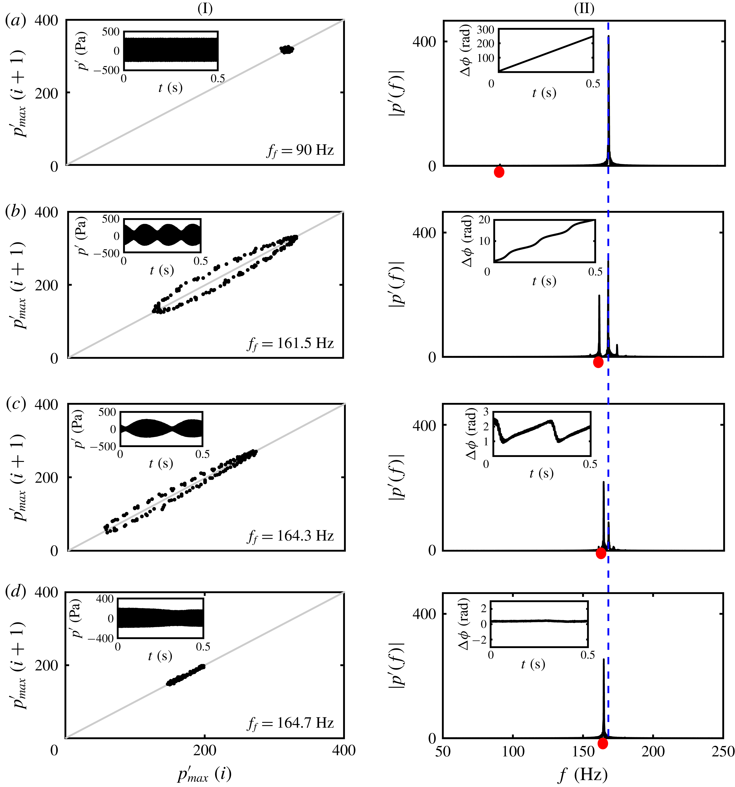
is varied. We observe different features of the forced synchronization and the response dynamics of the acoustic pressure. Representative states of synchronization and corresponding forced dynamics are shown for four different values of
 $f_{f}$
(figure 3).
As
 $f_{f}$
is varied towards
 $f_{n0}$
(168.8 Hz), we observe different dynamical states in the response signal (I) and different states of synchronization (II, inset) such as phase drifting (a,
 $f_{f}=90$
Hz), intermittent phase locking (b,
 $f_{f}=161.5$
Hz), phase trapping (c,
 $f_{f}=164.3$
Hz) and phase locking (d,
 $f_{f}=164.7$
Hz). Dynamics is presented by plotting the return map (I) and the corresponding time series (inset of I). Amplitude spectrum (forcing frequency is indicated by red dots) of the response signals (II) along with the relative phase dynamics (inset of II) are shown to identify the state of synchronization. The response frequency (
 $f_{r}$
) corresponding to natural oscillations is marked with a dashed line in the amplitude spectra.

The response dynamics of the acoustic pressure signals subjected to harmonic forcing can be inferred from the first return map (figure 3I) and the time series shown in figure 3I (inset). Further, the spectral properties such as frequency of the response signal (figure 3II) and instantaneous relative phase (calculated through Hilbert transform) between forcing and response signals are shown in figure 3II (inset). The forcing frequencies are indicated by red dots in the amplitude spectra (figure 3II).
When
 $f_{f}$
is 90 Hz (far from
 $f_{n0}$
, figure 3
aII), the dynamics of the response signal is insensitive to forcing (inset of figure 3
aI). The relative phase shows a continuous drift with time (inset of figure 3
aII), indicating that the forcing and the response oscillations are desynchronized.
When the value of
 $f_{f}$
(
 $=$
161.5 Hz) is close to
 $f_{n0}$
(figure 3
bII), the amplitude of the response signal shows modulation, known as beats (inset of figure 3
bI) with a beating frequency of
 $|\,f_{r}-f_{f}|$
, where
 $f_{r}$
is the response frequency. First return map of such modulated oscillations shows an oval shaped loop around the diagonal line, indicating two frequency oscillation. On the other hand, a staircase-like structure in the dynamics of the relative phase (inset of figure 3
bII) indicates a state of intermittent phase locking, where the spans of the phase locked states are separated by jumps (also referred to as phase slips) of integer multiples of
 $2\unicode[STIX]{x03C0}$
radians.
When
 $f_{f}$
(
 $=$
164.3 Hz) is very near to
 $f_{n0}$
, however, outside the phase-locking boundary (figure 3
cII), the relative phase indicates the presence of a phase trapping state, as inferred from the bounded and oscillatory behaviour of the relative phase. Such an oscillatory relative phase has a frequency equal to the beating frequency of the response signal (inset of figure 3
cII). Although the mean frequencies (
 $\unicode[STIX]{x1D714}=\langle \text{d}\unicode[STIX]{x1D719}/\text{d}t\rangle$
) of the forcing and the response signals are perfectly locked, the amplitude spectrum of the response signal still shows two distinct frequency peaks corresponding to
 $f_{f}$
and
 $f_{r}$
. This reflects in the beating structure of the response signal (inset of figure 3
cI), and a closed-loop structure along the diagonal line in the first return map (figure 3
cI).
During the onset of phase-locking state (
 $f_{f}=164.7$
Hz), the frequency peak corresponding to
 $f_{r}$
gets completely suppressed, thus showing a single peak at the forcing frequency (figure 3
dII). During this state, the relative phase fluctuates around a constant phase shift (inset of figure 3
dII) indicating a perfect locking of the instantaneous phases. The first return map corresponding to this state, hence, shows a cluster of points congregated along the diagonal line (figure 3
dI).
When
 $f_{f}$
is varied in such a way that it crosses the right boundary of the synchronization region (see Arnold tongue in figure 2), the observations of forced synchronization states such as phase trapping, intermittent phase locking and phase drifting are repeated in the response dynamics (not shown here for brevity).
4.2.2 Effect of the variation of forcing amplitude
We further investigate the effect of forcing amplitude on the response dynamics. Towards that purpose, we vary the forcing amplitude, maintaining the forcing frequency constant at
 $f_{f}=155$
Hz (significantly away from
 $f_{n0}$
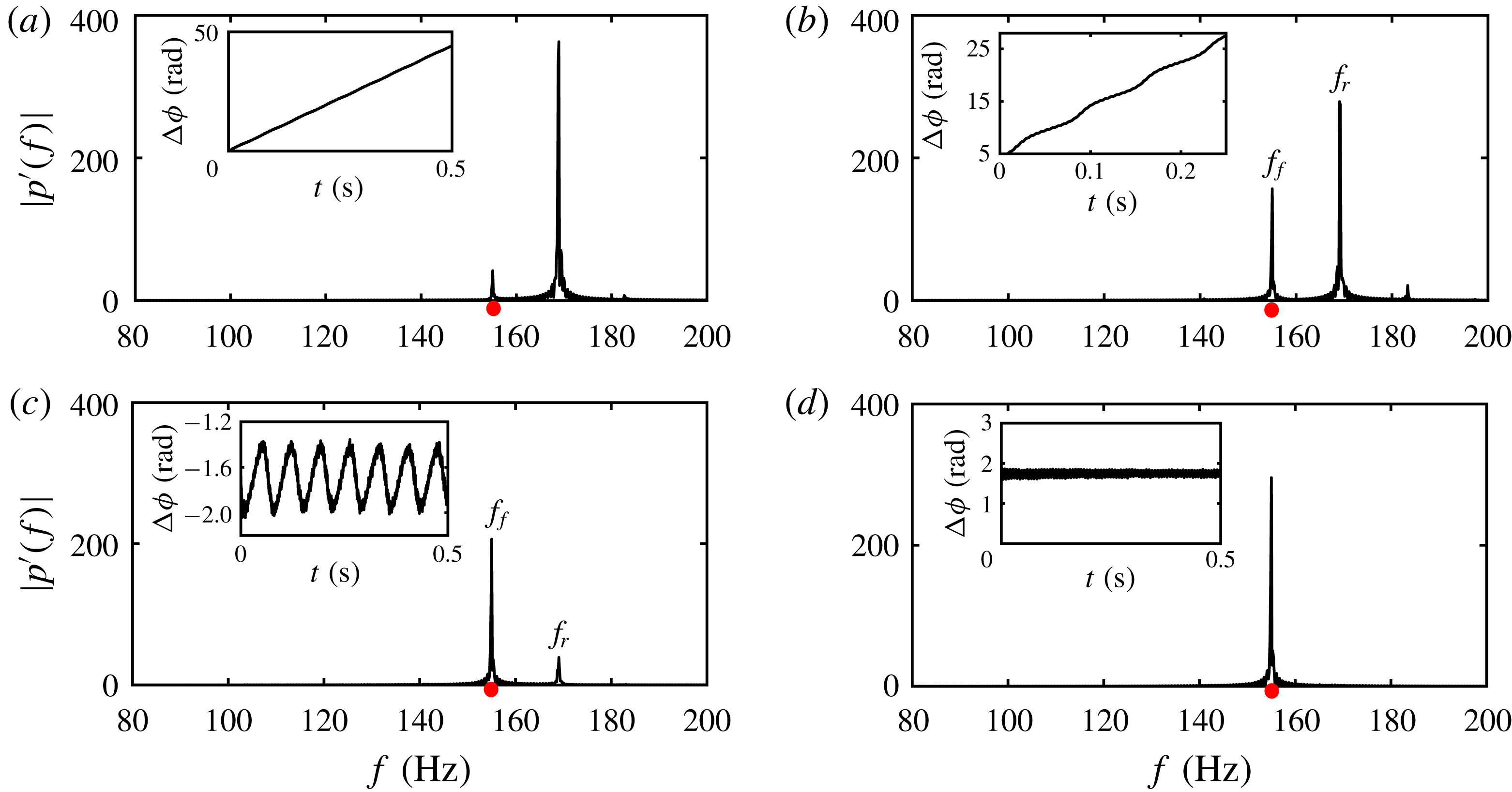
, chosen to look into different states of forced synchronization occurring through the mechanism of suppression, as shown in figure 4) and at
 $f_{f}=167.5$
Hz (very close to
 $f_{n0}$
, chosen to look into different states of forced synchronization occurring through the mechanism of phase locking, as shown in figure 5).
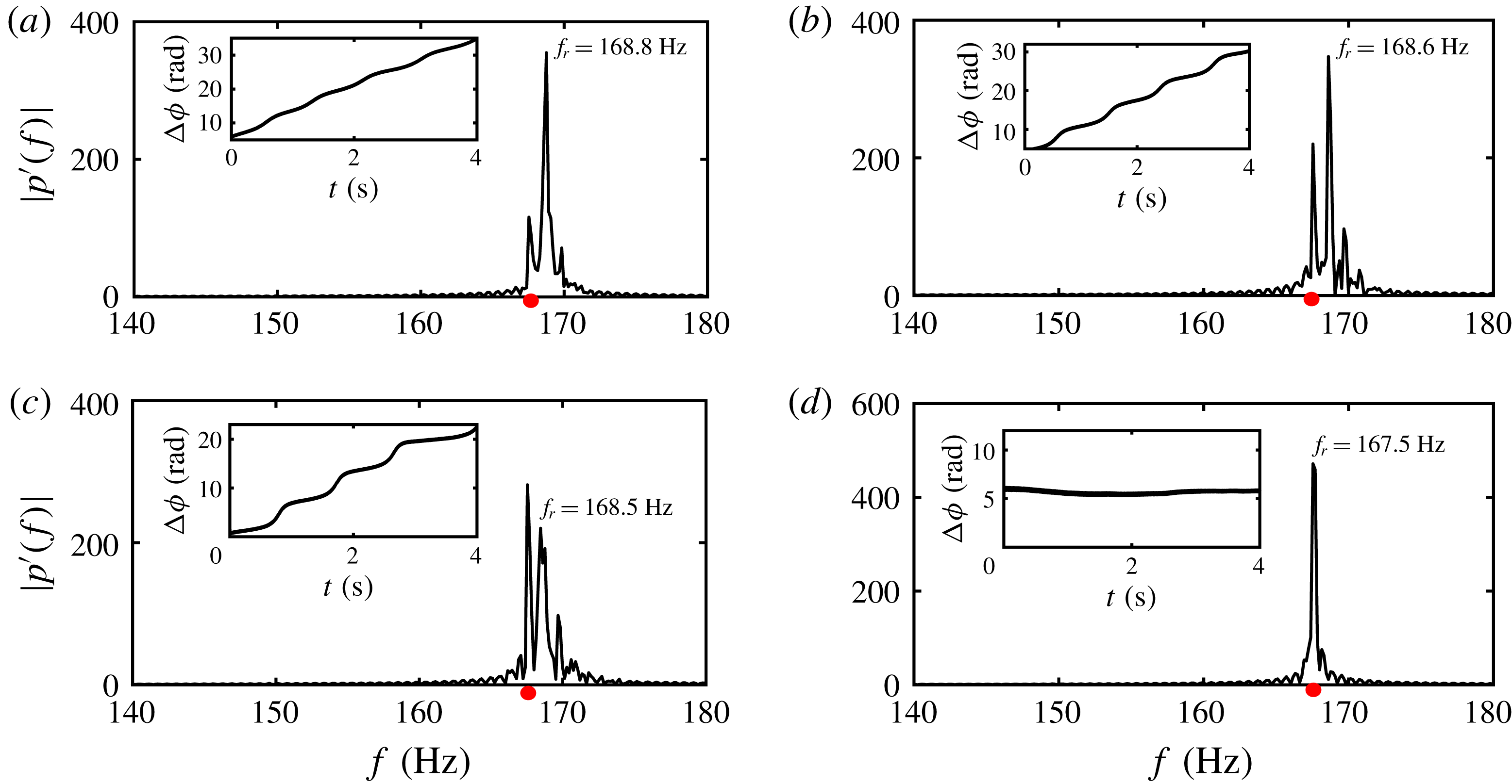
The plots show frequency spectra of the response signal, and temporal variation of the relative phase between the response dynamics and the forcing signal (insets) at different values of (a)
 $A_{f}=3$
mV, (b)
 $A_{f}=12$
mV, (c)
 $A_{f}=18$
mV and (d)
 $A_{f}=24$
mV, when
 $f_{f}$
is maintained constant at 155 Hz, which is sufficiently away from
 $f_{n0}$
(168.8 Hz). The red dot in the frequency spectra corresponds to the location of the forcing frequency (
 $f_{f}$
).

For
 $f_{f}=155$
Hz, when the amplitude of forcing is very small (
 $A_{f}=3$
mV), the external forcing does not affect the natural oscillations, resulting in a behaviour of phase drifting between the forcing and the response signals (inset of figure 4
a). With the increase of forcing amplitude to 12 mV, we observe a beating phenomenon (not shown here) in the amplitude of the response signal. This corresponds to a state of intermittent phase locking, confirmed from the observation of a wavy staircase-like structure in the relative phase dynamics (inset of figure 4
b). As we further increase
 $A_{f}$
(
 $A_{f}=18$
mV), we notice a shift in dominance of the peak frequencies from
 $f_{r}$
to
 $f_{f}$
in the amplitude spectrum (see figure 4
c). This results in the bounded nature of the relative phase, where the phase difference between the forcing and the response signals is trapped between finite values and oscillates in a periodic manner (inset of figure 4
c). When the forcing amplitude is sufficiently high (
 $A_{f}=24$
mV), we observe a perfect locking of instantaneous phases of the signals (inset of figure 4
d), wherein the natural oscillations get completely suppressed and the system oscillates with the forcing frequency (figure 4
d). Therefore, at
 $f_{f}=155$
Hz, forced synchronization occurs through the mechanism of suppression of natural oscillation (Balanov et al.
Reference Balanov, Janson, Postnov and Sosnovtseva2009).
For
 $f_{f}=167.5$
Hz, when
 $A_{f}$
is very small (0.4 mV, figure 5
a), the plot of relative phase shows a phase drifting behaviour, which subsequently transitions to a staircase-like structure at a higher value of the forcing amplitude (
 $A_{f}=0.8$
mV in figure 5
b). When
 $A_{f}=1.2$
mV, we notice a shift in the response frequency (
 $f_{r}$
) towards the forcing frequency (
 $f_{f}$
) as shown in figure 5(c). We, further, observe an intermittent phase-locking behaviour in the dynamics of the relative phase (inset of figure 5
c). When the amplitude of forcing is high (
 $A_{f}=1.7$
mV), the natural frequency eventually gets locked with the forcing frequency (inset of figure 5
d). Here, we notice that the transition from phase drifting to phase locking does not happen through phase trapping. The region of the Arnold tongue for which the state of phase trapping does not appear at the synchronization boundary (shown with a dashed circle in figure 2) is referred to as a phase locking region as forced synchronization occurs through the mechanism of phase locking in this region. The mechanisms of phase locking and suppression correspond to saddle-node and torus-death bifurcation, respectively (Balanov et al.
Reference Balanov, Janson, Postnov and Sosnovtseva2009). In the present study, we report the experimental observation of both the routes in a Rijke tube. Having characterized the different forced dynamics and synchronization behaviour, we now shift our attention to understand the effect of harmonic forcing on the amplitude of the response signal.
Plots showing amplitude spectra of the response signal, and instantaneous relative phase variation between the response and the forcing signal (insets), obtained for different values of
 $A_{f}=0.4$
mV (a), 0.8 mV (b), 1.2 mV (c) and 1.7 mV (d), when
 $f_{f}$
(167.5 Hz) is very close to
 $f_{n0}$
(168.8 Hz).

4.3 Effect of harmonic forcing on response amplitude
The overall amplitude of the forced system is referred to as the response amplitude from here on for brevity. Depending upon the choice of forcing parameters (i.e.
 $f_{f}$
and
 $A_{f}$
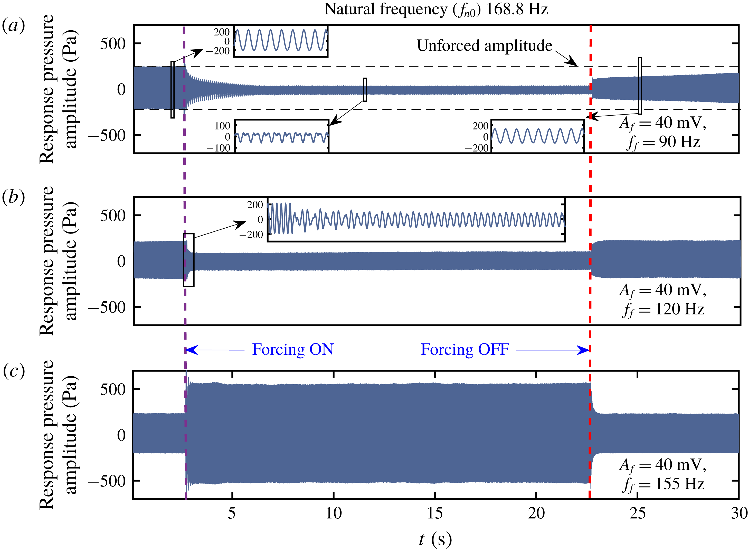
), the amplitude response of the system could be different. Typical time series of the acoustic pressure oscillations obtained in experiments for different values of forcing frequency are shown in figure 6. The time instances when the forcing is switched on and off are marked with violet and red dashed lines, respectively. The unforced pressure oscillation in the Rijke tube is periodic (see inset of figure 6
a) with an amplitude of nearly 215 Pa and a natural frequency of 168.8 Hz.
The time series of the acoustic pressure oscillations obtained from experiments showing the effect of forcing on the amplitude of the response signal for (a)
 $f_{f}=90$
Hz, (b)
 $f_{f}=120$
Hz and (c)
 $f_{f}=155$
Hz, keeping the forcing amplitude fixed at 40 mV. Depending upon the forcing frequency, the response oscillations can be quenched or amplified.

We vary
 $f_{f}$
starting from 90 Hz towards the natural frequency (168.6 Hz) keeping the forcing amplitude constant (40 mV). We find both reduction and increase in the response amplitude of forced oscillation depending upon the frequency of forcing. The acoustic pressure oscillations at forcing frequencies of 90, 120 and 155 Hz are shown in figure 6. When we force the system with a forcing frequency around 90 Hz, we find a maximum reduction in the response amplitude where the dynamics of the forced system does not exhibit sinusoidal oscillations (see inset of figure 6
a), indicating the existence of nonlinear interaction between the forced and the natural oscillations. We further note that the epoch of the initial transient in the signal after the forcing is switched on is long, i.e. around 5 s at
 $f_{f}=90$
Hz. Once the forcing is switched off, the system takes an even longer time to get back to the original unforced state of oscillation. At this forcing frequency, the thermoacoustic oscillations get destabilized due to the disturbance induced by the external forcing (the analysis is given in § 4.7). Therefore, once the forcing is switched off, the re-establishment of thermoacoustic oscillations takes a long time.
We find a reduction in the response amplitude even when
 $f_{f}=120$
Hz (figure 6
b). However, the reduction in amplitude is less compared to the previous case. Therefore, we believe that a low frequency forcing seems to be beneficial for mitigating thermoacoustic instability in practical systems to the extent that the system behaves like a periodic oscillator with a single dominant frequency. However, an experimental validation on more complicated thermoacoustic systems with many degrees of freedom needs to be performed. We further observe that the transient is short compared to the previous case and is aperiodic in nature (inset of figure 6
b). On the other hand, the forcing with a frequency (
 $f_{f}=155$
Hz) close to the natural frequency (
 $f_{n0}=168.8$
Hz) of the system leads to an amplification of the response signal (figure 6
c). This suggests that choosing a forcing frequency close to the natural frequency for controlling the thermoacoustic instabilities can be even more dangerous for the life of the systems.
Therefore, from a practical point of view, it is important to explore the effect of harmonic forcing on the response signal. The phenomena of reduction and amplification of the response signal can be understood with a careful analysis of the forcing and the self-excited oscillation separately.
4.4 Effect of harmonic excitation on the amplitudes of self-excited and forcing oscillations
We further analyse the effect of harmonic excitation on the amplitudes of the self-excited and the forcing oscillations separately. To that end, we obtain amplitudes of the self-excited oscillation (
 $A_{n}$
corresponding to the response frequency,
 $f_{r}$
) and that of the forcing (
 $A_{f}$
corresponding to the forcing frequency,
 $f_{f}$
) from the amplitude spectrum (by fast Fourier transform) of the response pressure signal. The normalized amplitudes (
 $A_{n}/A_{0}$
and
 $A_{f}/A_{0}$
) are plotted with the normalized forcing frequency (
 $f_{f}/f_{n0}$
), where
 $A_{0}$
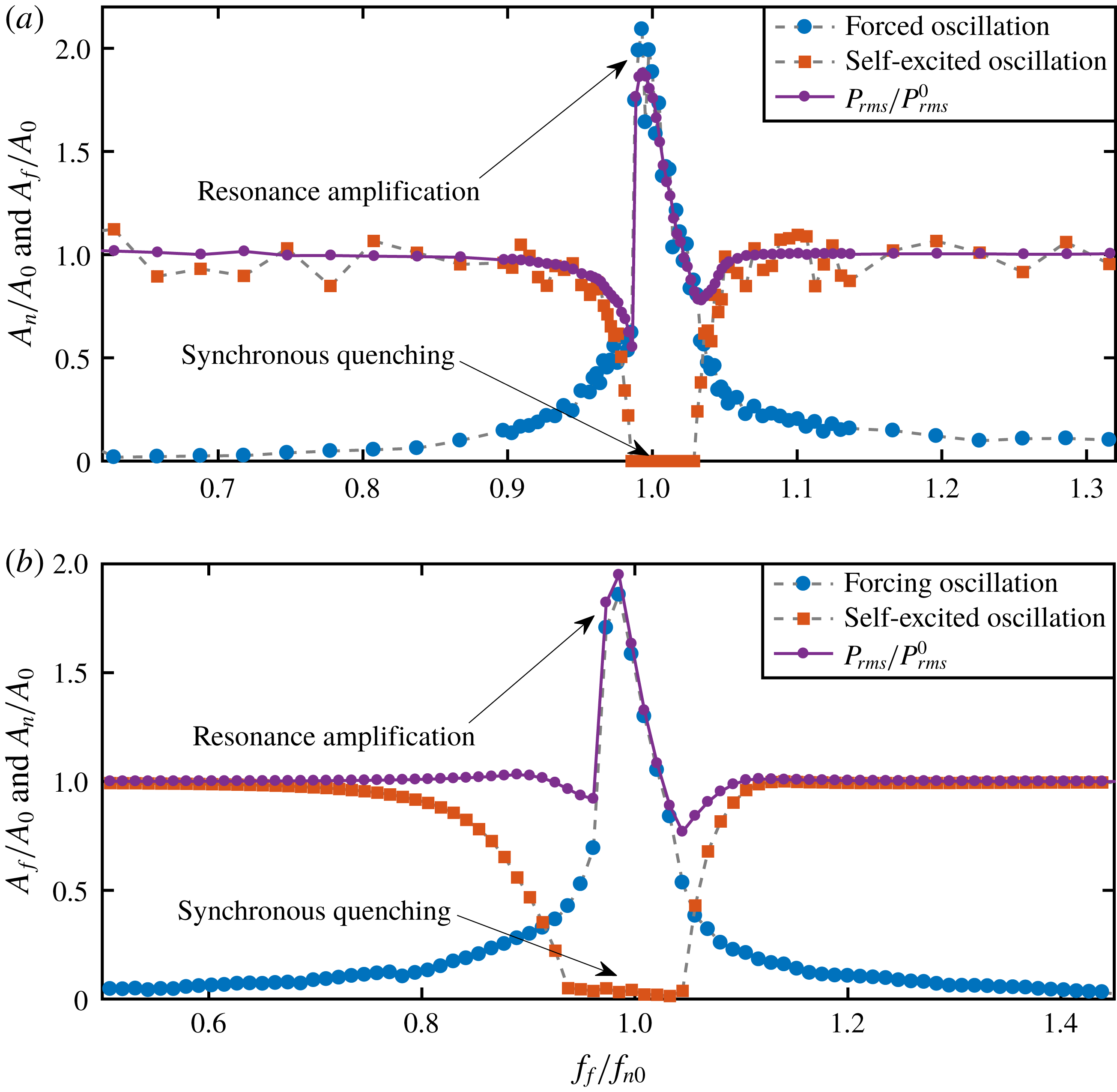
is the unforced spectral amplitude of the self-excited oscillations from both experimental data and model (figure 7). For this plot, the forcing frequency is varied, keeping the forcing amplitude constant (5 mV in experiment and 0.35 in model). We further plot the r.m.s. value of pressure oscillations obtained from experiments (figure 7
a) and from the model (figure 7
a) as we vary
 $f_{f}$
. We observe an asymmetry across the natural frequency in the amplitude response plots of the forced limit cycle oscillations. We further notice two distinct phenomena occurring simultaneously while
 $f_{f}/f_{n0}$
is close to 1.
Variation of spectral amplitude of self-excited oscillation (
 $A_{n}/A_{0}$
, in red squares) and of forcing (
 $A_{f}/A_{0}$
, in blue circles) when the forcing frequency is varied across the natural frequency of the Rijke tube at a constant value of forcing amplitude (
 $A_{f}=5$
mV in experiment and,
 $A_{f}=0.35$
in model), obtained from experiment (a) and model (b). Synchronous quenching of self-excited oscillations occurs when the forcing frequency (
 $f_{f}$
) is close to the natural frequency. This is associated with resonance amplification of the forcing signal. Due to the combined effects of synchronous quenching of the natural oscillation and resonant amplification of the forcing, there is an overall amplification in the
 $P_{rms}/P_{rms}^{0}$
value of the response signal (a,b) where
 $P_{rms}^{0}$
is the r.m.s. value of unforced pressure oscillation.

The amplitude corresponding to the self-excited oscillations (
 $A_{n}/A_{0}$
) shows a gradual decrease as
 $f_{f}/f_{n0}$
approaches 1. Such reduction in the amplitude of self-excited oscillations occurs due to the phenomenon of synchronous quenching until the onset of phase locking is observed (figures 7
a and 7
b, represented in red squares). In the regime of frequency or phase locking of the Arnold tongue (shown in figure 2), the spectral amplitude of self-excited oscillations is completely suppressed. In the same regime of frequency ratio, the amplitude of forced oscillation (
 $A_{f}/A_{0}$
) initially shows a gradual increase as
 $f_{f}/f_{n0}$
approaches 1 (figures 7
a and 7
b, represented in blue circles) and then exhibits a sudden jump to a very large amplitude at the onset of phase locking due to the effect of resonance amplification (Odajima et al.
Reference Odajima, Nishida and Hatta1974; Ohe & Takeda Reference Ohe and Takeda1974; Abel et al.
Reference Abel, Ahnert and Bergweiler2009). Thus, the simultaneous occurrence of synchronous quenching of natural oscillations and resonance amplification of the forcing signal makes the response signal dominated by the forcing signal. This, in turn, results in the phase locking between the forcing and the response signals. Further, due to the combined effects of synchronous quenching of natural oscillations and resonant amplification of forcing, the r.m.s. value of the response pressure oscillation shoots up to a very high value, compared to the unforced amplitude of the signal, in the synchronization region and then exhibits a gradual decrease with the further increase in
 $f_{f}/f_{n0}$
(violet curve in figure 7
a). We call this shooting up of the response amplitude (around
 $f_{f}=f_{n0}$
) synchronance (synchronization–resonance). Such simultaneous occurrence of synchronization and resonance in the frequency locking region has also been reported by Abel et al. (Reference Abel, Ahnert and Bergweiler2009) who conducted experiments with a self-excited organ tube forced externally using a loudspeaker. Further, we notice that when the value of forcing frequency is far away from
 $f_{n0}$
, the amplitude of natural oscillations is not affected by the forcing, and thereby, the r.m.s. value of the response signal is also unaltered.
4.5 Effect of forcing on the response amplitude
We further examine the r.m.s. value of response pressure oscillation when
 $A_{f}$
is varied keeping
 $f_{f}$
fixed at different values. Four values of
 $f_{f}$
are chosen in such a manner that two of them are close to
 $f_{n0}$
and the other two are relatively further away from
 $f_{n0}$
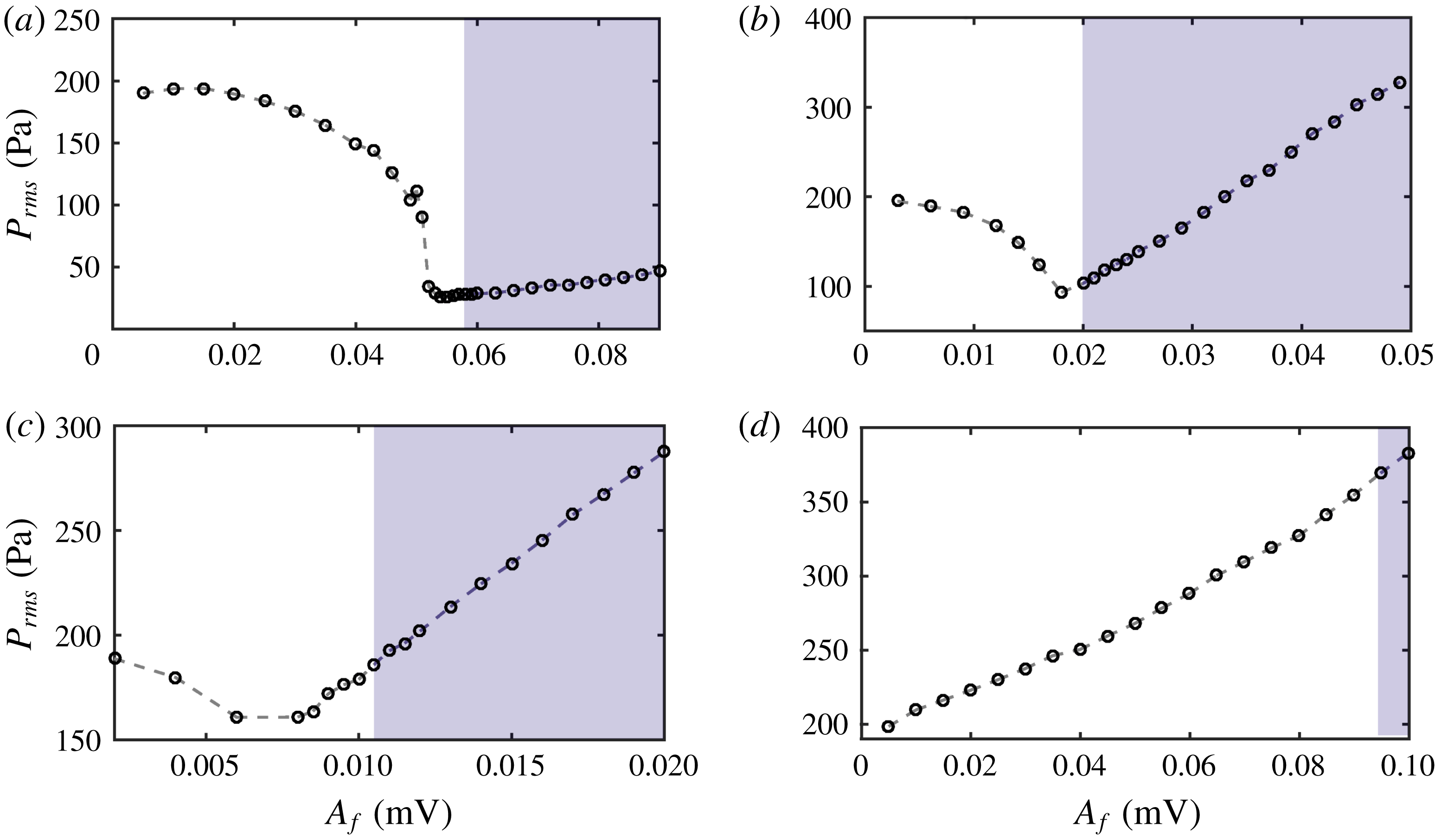
. We observe that the response amplitude of the acoustic pressure first decreases to a minimum value prior to exhibiting a linear increase, which is primarily due to the gradual increase in the forcing amplitude. This behaviour is observed for
 $f_{f}<f_{n0}$
(figure 8
a,b) and also for
 $f_{f}>f_{n0}$
only when the frequency detuning is small (figure 8
c). This reduction in the amplitude of the acoustic pressure signal is not observed when
 $f_{f}$
is significantly larger than
 $f_{n0}$
(figure 8
d), wherein the response amplitude shows a continuously increasing trend without any minima. From the analysis of relative phase between the forcing and the forced oscillations, as shown in figures 4 and 5, we notice that the minimum in the plot of response amplitude (see figure 8) is close to the boundary of the phase-locking regime (shown as the shaded portion in figure 8
a–c). In the region of perfect phase locking, the response amplitude of the acoustic pressure oscillations demonstrates almost a linear growth with an increase in
 $A_{f}$
. Such a growth of the response amplitude of pressure signal in the synchronization region is significantly steep when
 $f_{f}$
is close to
 $f_{n0}$
(figure 8
b,c). This rapid amplification of the r.m.s. values of response pressure oscillations when
 $f_{f}/f_{n0}$
approaches 1 happens due to the phenomenon of synchronance as explained earlier in figure 7. However, the growth in the response amplitude of the pressure signal in the synchronization region is moderate when
 $f_{f}$
is much lower than
 $f_{n0}$
(figure 8
a). We further notice that the minimum value of the response amplitude, observed prior to the onset of perfect phase-locking state, increases as
 $f_{f}$
is increased.
The variation of response amplitude (
 $P_{rms}$
) of the acoustic pressure signals obtained from experiments as
 $A_{f}$
is varied for different
 $f_{f}=100$
Hz (a), 155 Hz (b), 175 Hz (c) and 200 Hz (d). Reduction in response amplitude is observed for all forcing frequencies except when
 $f_{f}$
is sufficiently higher than
 $f_{n0}$
(d). The shaded region indicates the zone of phase locking.

4.6 Characterization of maximum reduction in the response amplitude due to harmonic forcing
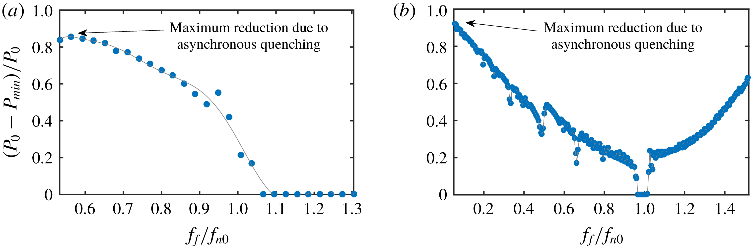
The reduction in the r.m.s. value of the response pressure signal due to harmonic forcing is shown in figure 9 when we vary
 $f_{f}$
across
 $f_{n0}$
, and for each value of
 $f_{f}$
we further vary
 $A_{f}$
to obtain the minimum amplitude for that particular
 $f_{f}$
. Suppression (
 $P_{0}-P_{min}$
) in the amplitude of the response signal is normalized with the r.m.s. value of the unforced natural oscillation (
 $P_{0}$
), where
 $P_{min}$
represents the minimum r.m.s. value of the response signal achieved while
 $A_{f}$
is varied for each value of
 $f_{f}$
. We observe the maximum reduction in the amplitude of the response signal when
 $f_{f}$
is significantly lower than the natural frequency (
 $f_{n0}$
). As we move towards
 $f_{n0}$
, the amount of amplitude reduction gradually decreases (figure 9
a). This also suggests that the effectiveness of forcing in suppressing the amplitude of the unforced oscillation decreases as
 $f_{f}$
approaches
 $f_{n0}$
.
Amplitude reduction as a function of normalized forcing frequency (
 $f_{f}/f_{n0}$
) obtained from experiments (a) and model (b) representing the maximum decrease in overall response amplitude of the acoustic pressure signal when
 $f_{f}$
is varied across
 $f_{n0}$
. The amplitude reduction (
 $P_{0}-P_{min}$
) is normalized with the r.m.s. value of the unforced amplitude (
 $P_{0}$
), where
 $P_{min}$
represents the minimum r.m.s. value achieved while
 $A_{f}$
is varied for a particular value of
 $f_{f}$
.

We do not observe any reduction in the response amplitude when
 $f_{f}>f_{n0}$
in experiments (figure 9
a). In other words, when
 $f_{f}>f_{n0}$
, the r.m.s. value of the response signal does not reduce at all as
 $A_{f}$
is varied (see figure 8
d). Similar observation has been mentioned in Lubarsky et al. (Reference Lubarsky, Shcherbik, Zinn, McManus, Fric and Srinivasan2003), Bellows et al. (Reference Bellows, Hreiz and Lieuwen2008) and Abel et al. (Reference Abel, Ahnert and Bergweiler2009). Amplification of the forcing signal has been found in a system of self-excited organ pipe for
 $f_{f}>f_{n0}$
(Abel et al.
Reference Abel, Ahnert and Bergweiler2009) and in a laminar flame combustor for
 $f_{f}<f_{n0}$
as well as
 $f_{f}>f_{n0}$
(Guan et al.
Reference Guan, Gupta, Kashinath and Li2018). Thus, forcing the limit cycle oscillation at a frequency greater than the natural frequency of the oscillations might not lead to a significant suppression of the overall amplitude of the limit cycle, depending on the thermoacoustic system involved.
When
 $f_{f}/f_{n0}$
is around 0.6, i.e. the forcing frequency is near the subharmonic frequency of natural oscillations (
 $f_{n0}/2$
), the reduction in response amplitude of the limit cycle oscillations in the system reaches almost 80 % of their unforced amplitude (figure 9
a). Such a suppression in natural oscillation that occurs when
 $f_{f}$
is significantly away from
 $f_{n0}$
is due to the phenomenon of asynchronous quenching (Minorsky Reference Minorsky1967; Staubli Reference Staubli1987). During asynchronous quenching, we notice that the minimum amplitude achieved through forcing is close to that of the imposed forcing amplitude. Therefore, we suggest that the occurrence of asynchronous quenching through the proper choice of forcing parameters can be effective in mitigating the amplitude of thermoacoustic instability while forced at a frequency much lower than the natural frequency.
On performing a similar analysis in the model, we observe a reduction in the response amplitude of as high as 95 % of the unforced amplitude when
 $f_{f}/f_{n0}$
is
 ${\sim}0.03$
(figure 9
a). Therefore, the model chosen in this study is able to capture the phenomenon of amplitude reduction due to asynchronous quenching qualitatively, but not quantitatively. Further, the amplitude reduction of the response signal is found even when the system is forced with
 $f_{f}>f_{n0}$
(figure 9
b). The phenomenon of asynchronous quenching occurring at both
 $f_{f}/f_{n0}<1$
and
 $f_{f}/f_{n0}>1$
is not observed in the present experimental set-up. However, using a laminar flame combustor, Guan et al. (Reference Guan, Gupta, Kashinath and Li2018) showed the existence of asynchronous quenching for
 $f_{f}<f_{n0}$
as well as
 $f_{f}>f_{n0}$
, which qualitatively corroborates the forced Duffing–van der Pol oscillator with weak nonlinearity.
4.7 Physical explanation for the amplitude suppression due to asynchronous quenching
As the phenomenon of thermoacoustic instability is a consequence of positive coupling between the acoustic pressure (
 $p^{\prime }$
) and the heat release rate (
 $\dot{q}^{\prime }$
) oscillations, it is critical to explore the effect for harmonic forcing on such thermoacoustic coupling. As we do not have a means to measure
 $\dot{q}^{\prime }$
(3.10) in the present experimental facility of the Rijke tube, we try to find a plausible explanation from the model that governs the essential features of this system.
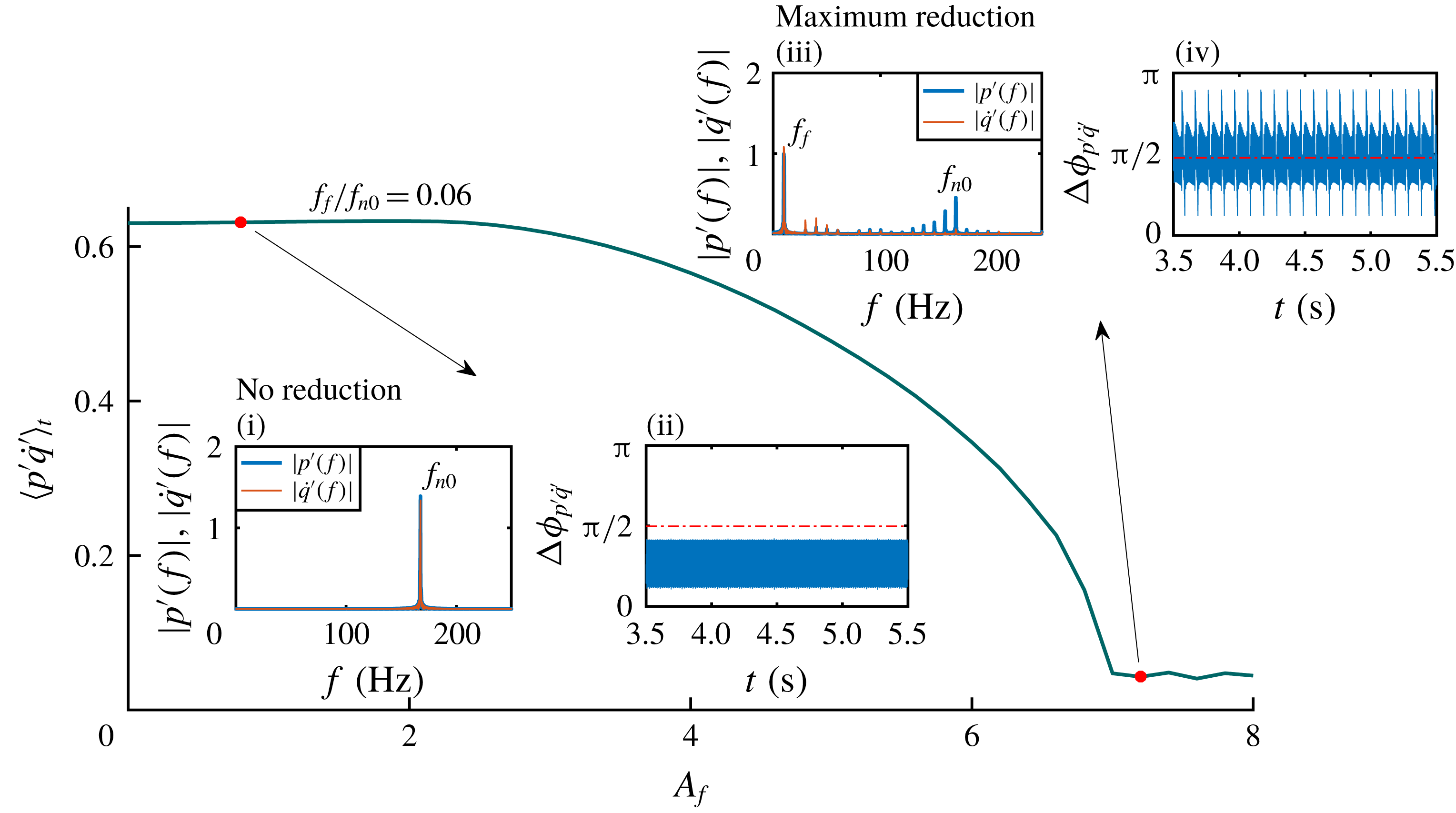
Cycle-averaged value of the acoustic power production (
 $\langle p^{\prime }\dot{q}^{\prime }\rangle _{t}$
;
 $t=512$
× time period) is plotted for a low forcing frequency (
 $f_{f}/f_{n0}=0.06$
) and by varying the amplitude of forcing (
 $A_{f}$
) in the model. Both
 $p^{\prime }$
and
 $\dot{q}^{\prime }$
are normalized to zero mean and unit variance, and their product is averaged over 512 cycles. Amplitude spectra of
 $p^{\prime }$
and
 $\dot{q}^{\prime }$
and the relative phase between them are shown for two different
 $A_{f}$
(indicated as red dots) corresponding to the instants of ‘no reduction’ and ‘maximum reduction’.

The phenomena of synchronous quenching and asynchronous quenching are well captured in the present model of the Rijke tube (refer to figures 7
b and 9
b, respectively). Further, the association of resonance amplification of the forcing signal with the synchronous quenching of self-excited oscillations is also well predicted in the model (figure 7
b). Therefore, in the model, we look into the normalized and cycle-averaged acoustic power production,
 $\langle p^{\prime }\dot{q}^{\prime }\rangle _{t}$
(where
 $t=512$
× time period), which is responsible for the sustenance of thermoacoustic instability (Lieuwen & Yang Reference Lieuwen and Yang2005).
The variation of
 $\langle p^{\prime }\dot{q}^{\prime }\rangle _{t}$
with
 $A_{f}$
is shown in figure 10. Here, we choose a forcing frequency (
 $f_{f}/f_{n0}=0.06$
) at which the model shows significant reduction in the r.m.s. value of the pressure oscillations (figure 9
b). With an increase in
 $A_{f}$
,
 $\langle p^{\prime }\dot{q}^{\prime }\rangle _{t}$
decreases (figure 10) and becomes minimum when we achieve maximum reduction in the amplitude of pressure oscillation. The low value of acoustic driving (
 $\langle p^{\prime }\dot{q}^{\prime }\rangle _{t}$
) explains the reduction in the amplitude of self-excited oscillation observed during thermoacoustic instability. Further, we observe that, at the instant of no amplitude reduction, the acoustic pressure and the heat release rate oscillate at the natural frequency (figure 10i) and their relative phase oscillates within 0 and
 $\unicode[STIX]{x03C0}/2$
rad (figure 10ii), satisfying the Rayleigh criterion (Rayleigh 1878). On the other hand, at the instant of maximum amplitude reduction, both the acoustic pressure and the heat release rate oscillations have a dominant peak at the forcing frequency (figure 10iii), and therefore, they are phase locked, which can be inferred from the bounded relative phase shown in figure 10(iv). Interestingly, at this condition of forcing, the relative phase between
 $p^{\prime }$
and
 $\dot{q}^{\prime }$
oscillates around
 $\unicode[STIX]{x03C0}/2$
rad, which according to the Rayleigh criterion will lead to an alternative acoustic driving and damping (figure 10iv). This, in turn, is manifested as a very low value (
 $=$
0.045) of
 $\langle p^{\prime }\dot{q}^{\prime }\rangle _{t}$
(corresponding to an average phase difference,
 $\langle \unicode[STIX]{x0394}\unicode[STIX]{x1D719}_{p^{\prime }\dot{q}^{\prime }}\rangle _{t}$
, of
 $0.49\unicode[STIX]{x03C0}$
) compared to the value (0.63) of
 $\langle p^{\prime }\dot{q}^{\prime }\rangle _{t}$
during thermoacoustic instability (figure 10). This observation suggests a plausible physical mechanism behind the quenching of thermoacoustic instabilities due to forcing, which mainly happens due the destruction of the positive interaction between
 $p^{\prime }$
and
 $\dot{q}^{\prime }$
when a high amplitude forcing is applied at the low value of frequency. In summary, asynchronous quenching, which is a characteristic phenomenon of a harmonically forced limit cycle oscillator, appears promising in practical and more complex thermoacoustic systems to suppress the unwanted high amplitude pressure oscillations.
5 Conclusions
We perform both theoretical and experimental investigation of forced synchronization in a simple thermoacoustic system, the horizontal Rijke tube. By varying the forcing frequency and the forcing amplitude, we observe the phenomenon of 1 : 1 synchronization both in the experiments and the model. We further identify different states of synchronization between the response signal and the forcing signal when the forcing amplitude and the forcing frequency are individually varied. When the system is forced with a frequency which is close to its natural frequency, the concurrence of both synchronous quenching of natural oscillations and resonance amplification of the forcing signal is observed along with different states of forced synchronization. On the other hand, as the forcing frequency (
 $f_{f}$
) is fairly lower than the natural frequency (
 $f_{n0}$
) of the system, a substantial amount of amplitude reduction (almost 80 % of the unforced amplitude in experiments) occurs due to the phenomenon of asynchronous quenching. Such phenomena are usually disregarded by ascribing the dynamics to the ‘nonlinear interaction’ between the forcing and the self-sustained oscillations without going into details. This is the first study to recognize the maximum reduction in the amplitude is due to the occurrence of asynchronous quenching. We found that asynchronous quenching is associated with the breaking of positive coupling between the acoustic pressure and the heat release rate oscillations in the thermoacoustic system when forced at frequencies considerably lower than their natural frequency of oscillation. The phenomenon of asynchronous quenching found its applications in ion-sound instability (Keen & Fletcher Reference Keen and Fletcher1969) and self-excited ionization waves (Ohe & Takeda Reference Ohe and Takeda1974). Quenching of oscillation amplitude in practical thermoacoustic systems such as gas turbine engines is desirable and the occurrence of asynchronous quenching can be helpful for such systems. However, the experimental validity of asynchronous quenching for more complicated thermoacoustic systems (for example, turbulent combustors) with many degrees of freedom needs further investigation. Furthermore, similar characteristics of quenching may be expected in other hydrodynamically self-sustained oscillations as well.
Acknowledgements
The lead author gratefully acknowledges the Institute Post-doctoral Fellowship of the Indian Institute of Technology Madras, India. This work was supported by the Office of Naval Research Global (contract monitor: Dr R. Kolar; grant no. N62909-18-1-2061). The authors also acknowledge the help of Thilagraj for drawing the schematic of the experimental set-up.