



1. Introduction
Viscous fingering (VF) is a hydrodynamic interfacial instability, which is ubiquitous in various porous media flows during the displacement of a more viscous fluid by a less viscous one (Homsy Reference Homsy1987). The two fluids may be miscible or immiscible in nature. The less viscous fluid may displace the more viscous one linearly or radially, and accordingly the fingering instability is termed as rectilinear VF (Tan & Homsy Reference Tan and Homsy1988; Mishra, Martin & De Wit Reference Mishra, Martin and De Wit2008) or radial VF (Tan & Homsy Reference Tan and Homsy1987; Chen et al. Reference Chen, Huang, Gadêlha and Miranda2008; Sharma et al. Reference Sharma, Pramanik, Chen and Mishra2019). Viscous fingering is observed in various applications such as chromatographic separations (De Wit, Bertho & Martin Reference De Wit, Bertho and Martin2005; Guiochon et al. Reference Guiochon, Felinger, Shirazi and Katti2008), spreading of pollution zones in aquifers (Kretz et al. Reference Kretz, Berest, Hulin and Salin2003; De Wit et al. Reference De Wit, Bertho and Martin2005) or in mixing during brine transport in aquifers. In all these displacement processes, it is possible that a finite amount of more or less viscous fluid gets displaced in the porous medium by another bulk fluid resulting in a limited amount of one of the fluids.
Understanding how VF effects or is affected by the finite amount of an intermediate fluid sandwiched between two semi-infinite regions of another fluid has been of keen interest to many researchers. For instance, De Wit et al. (Reference De Wit, Bertho and Martin2005) considered VF of a high viscous slice displaced linearly by a less viscous fluid and observed that in comparison to the fingering between semi-infinite regions, VF of finite slice is a transient phenomenon which is a consequence of the decrease in viscosity with time. They observed an increase in the variance due to the broadening of the peak as a result of VF. This indicates that one fluid present in limited amounts does effect the fingering dynamics and VF with two interfaces always has properties different from VF with a single interface. Further, Mishra et al. (Reference Mishra, Martin and De Wit2008) compared the rectilinear fingering dynamics by considering the slice to be more as well as less viscous than the ambient displacing fluid, and reported that the variance of the less viscous sample is larger than that of the more viscous sample. Such displacement of the finite solute plug of greater or lesser viscous fluid by a less viscous fluid in chromatography column develops fingering instability, respectively, at the rear or frontal interface, and is captured in classical experiments by Shalliker et al. (Reference Shalliker, Catchpoole, Dennis and Guiochon2007) and Mayfield et al. (Reference Mayfield, Shalliker, Catchpoole, Sweeney, Wong and Guiochon2005).
Further, a physiochemical aspect of finite width of a solute plug, i.e. the effects of linear and nonlinear adsorption phenomena in the miscible VF, has been thoroughly explored in the literature theoretically (Edstrom, Samuelsson & Fornstedt Reference Edstrom, Samuelsson and Fornstedt2011; Rana et al. Reference Rana, Pramanik, Martin, De Wit and Mishra2019), and the interaction of unstable and stable interfaces to control the dynamical fingering patterns due to adsorption is observed. Hota, Pramanik & Mishra (Reference Hota, Pramanik and Mishra2015) performed a numerical linear stability analysis to understand how linear adsorption isotherm affects onset of instability in a finite slice, and succeeded in capturing the diffusion dominated region during early stages of the flow process. So far, we have mentioned VF by considering the displacement of the slice of a fluid sandwiched between another fluid having different viscosity in the presence or absence of adsorption. However, the finite extent of fluids can be of arbitrary shape (Pramanik, De Wit & Mishra Reference Pramanik, De Wit and Mishra2015), may be present in the entire domain (Jha, Cueto-Felgueroso & Juanes Reference Jha, Cueto-Felgueroso and Juanes2011) or there may be three different fluids with one fluid confined between the other two (Daripa & Gin Reference Daripa and Gin2016). One thing common in these studies is rectilinear displacement of a miscible fluid by another of different viscosity. However, Cardoso & Woods (Reference Cardoso and Woods1995) considered a three layer system containing an immiscible layer of fluid bounded by two other fluids both for linear and radial displacement. They reported a stabilisation of the system due to continuous thinning of the intermediate layer in the radial displacement while the layer breaks into drops for rectilinear displacement. In context with radial displacement of the miscible fluids, Chen et al. (Reference Chen, Huang, Huang and Miranda2015) considered alternate injection of the more and the less viscous fluids and found that multiple interfaces helped enhance the mixing of the fluids.
The two-interface problems (stable–unstable or unstable–unstable ones) have applications in polymer flooding in the enhanced heavy oil recovery processes (Vishnudas & Chaudhuri Reference Vishnudas and Chaudhuri2017). Zhou, Dong & Maini (Reference Zhou, Dong and Maini2013) performed experiments to understand the enhanced heavy oil recovery by chemical flooding through a rectilinear displacement process by conducting various chemical slug injections in a two-dimensional sand-packed cell. They used one chemical slug and two chemical slug tests, and showed that the second polymer slug injection can recover more oil if a water slug injection is applied between the two chemical slugs. Further Chaudhuri & Vishnudas (Reference Chaudhuri and Vishnudas2018), analysed the polymer flooding processes through a radial displacement in one-quarter of a five-spot system by considering a miscible polymer intermediate layer between water and oil as innermost and outermost fluids, respectively. Such a model gives rise to a system with miscible viscous fingers piercing out to the polymer bank, and further entering the immiscible outward interface at the polymer and oil bank. They reported that, with the non-uniform flow phenomenon in a five-spot set-up, the fingering patterns are very much different than they are in a rectilinear displacement. This describes that, not only the pattern formation but also the complete interfacial VF dynamics of the two-interface problem can be changed depending on the nature of the displacement, i.e. whether radial or rectilinear.
Recently, in context with the treatment of fluids in an oil well, Beeson-Jones & Woods (Reference Beeson-Jones and Woods2015) considered the overall stability of the radially spreading annulus considering three fluids each having different viscosity. They reported that the results for an annulus are similar to the single interface radial flow, but depend on the viscosity difference between the inner and outer fluid. To the best of our knowledge, no study exists with miscible fluids, and hence no conclusion can be drawn if miscibility also plays a role in addition to the interaction of fronts existing due to one fluid being limited between the other two. This motivates us to understand the miscible VF with an annular ring with the following two purposes: (i) to understand the analogy and differences between the VF with a slice and VF with an annulus; (ii) if the results known for classical radial VF are affected due to the confinement of one of the fluids. For the sake of simplicity, we consider only two fluids, with the more viscous annulus bounded between two layers of the less viscous fluid, so that only one interface is unstable, while the other spreads diffusively.
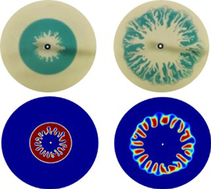
Throughout the study, we ask and answer the following questions. How miscible VF is affected if we consider radial displacement with one of the fluids confined between layers of another fluid? Is the instability thus obtained a transient phenomenon or the non-uniform radial velocity results in different dynamics? How does the competition between the convection and diffusion (Sharma et al. Reference Sharma, Nand, Pramanik, Chen and Mishra2020) affect VF of a miscible annulus? In an attempt to answer these questions, we consider the VF of an annulus of a more viscous fluid bounded by inner and outer regions of less viscous fluids. Such an annulus is formed by the radial displacement of a finite amount of high viscous intermediate fluid by a less viscous inner fluid. Various facets of miscible VF with the finiteness of the intermediate fluid are analysed by performing experiments, and further explained with the help of nonlinear simulations. It is observed that in contrast to rectilinear VF with a slice, fingers always remain in the present case. However, after some time, fingers evolve as frozen fingers without generation of new fingers. Also, first of its type, variance is found to be a non-monotonic function of time, which is a consequence of the limited more viscous fluid and the competition between the two opposing forces of convection and diffusion. The minimum in the variance curve is explained in terms of the distorted pressure contours indicating the interaction of the two fronts, even before the fingers touch the stable interface.
The paper is organised so as to simultaneously understand the experimental and the numerical results. The mathematical model followed by the numerical method is discussed in § 2. The experimental set-up, as well as the fingering dynamics of miscible annulus of the intermediate fluid between the inner and outer fluids, is presented in § 3. A thorough quantitative understanding of the computational results with different parameters of VF of a miscible annular ring, along with the corresponding experimental validations, is made in § 4, followed by the conclusions in § 5.
2. Mathematical formulation
2.1. Mathematical model
We consider a two-dimensional flow of Newtonian, incompressible, miscible and non-reactive fluids in a homogeneous porous medium. With an aim to understand VF of a miscible annular ring, we generate an annulus of one fluid which we call a sample fluid (De Wit et al. Reference De Wit, Bertho and Martin2005), with viscosity  $\mu _s$, surrounded by the other fluid which is referred to as the carrier fluid, having viscosity
 $\mu _c$ and radially displacing the sample. In order to model the radial (point source) flow to replicate the experimental conditions and to validate the experiments discussed in § 3, we use the two-phase Darcy law (TPDL) module of COMSOL (COMSOL Multiphysics
 $^{\circledR}$). The computational domain constitutes the region between two concentric circles of radii
 $r_{in}, r_{out}$ (see figure 1 for a schematic of the flow problem). The computations are performed in Cartesian coordinates with the origin being the centre of the two circles. The inner smaller circle acts as an injection hole to inject the fluid. The presence of this hole helps replicate the experimental conditions and avoids any singularity in the velocity (Chen et al. Reference Chen, Huang, Gadêlha and Miranda2008; Sharma et al. Reference Sharma, Pramanik, Chen and Mishra2019) at the origin, which is out of the domain.
Schematic of the computational domain. The white circle in the centre represents the injection hole with radius  $r_{in} = 2\ \textrm {mm}$.

Below, we briefly explain how the equations in the TPDL module can be utilised to model the single-phase porous media flow of miscible fluids. A detailed description of the same is available in one of our previous works (Sharma, Pramanik & Mishra Reference Sharma, Pramanik and Mishra2017). Under the assumption of constant density of the fluids and disregarding the gravity and capillary pressure, the equations in the TPDL module are
 \begin{gather} \boldsymbol{\nabla}\boldsymbol{\cdot} \boldsymbol{u} = 0, \end{gather}
 \begin{gather}\boldsymbol{u} ={-}\frac{\kappa}{\mu} \boldsymbol{\nabla} p, \end{gather}
 \begin{gather}\frac{1}{\mu} = s_1 \frac{\kappa_{r_1}}{\mu_1} + s_2 \frac{\kappa_{r_2}}{\mu_2}, \end{gather}
 \begin{gather}\frac{\partial \epsilon_p s_1}{\partial t} + \boldsymbol{u} \boldsymbol{\cdot} \boldsymbol{\nabla} s_1 = D \nabla^2{s_1}, \end{gather}
where  $\boldsymbol {u} = (u,v)$ is the Darcy velocity,
 $p$ is the hydrodynamic pressure,
 $\kappa$ and
 $\epsilon _p$ are, respectively, the permeability and porosity of the porous medium. Here
 $\kappa _{ri}, s_i, i = 1, 2,$ are the relative permeabilities and the saturation of the two fluids and
 $D$ is the capillary diffusion. Also,
 $s_1+s_2=1$ so that the medium is completely saturated. The experiments in this paper are performed using a water–glycerol system. Thus, in our numerical simulations, we consider the second fluid to be water and define the concentration of the species (glycerol) to be
 $c= \rho _1(1-s_2)=\rho _1 s_1$. However,
 $\rho _1$ can be assigned arbitrary values as density is assumed to play no role in our study. Without loss of generality, we assume
 $\rho _1$ to be unity so that the species concentration is given as
 $c=s_1$ which can be obtained by solving equation (2.4). Thus,
 $D$ can be regarded as the molecular diffusion coefficient of glycerol in water, and we use
 $s_1$ to represent the species concentration. Equation (2.4) is associated with the following initial condition:
 \begin{equation} s_1(x, y, t = 0) = \left\{\begin{array}{@{}ll} 1, & r_{in}^2 < x^2 + y^2 \leqslant r_1^2 \\ 0, & \mbox{otherwise,} \end{array} \right . \end{equation}
where  $r_1$ is the radius of the circle occupied by the sample fluid initially, and
 $r_{in}$ is the radius of the injection hole. The carrier fluid is continuously injected through the injection hole at a constant velocity
 $U_0$, specified as
 \begin{equation} - \hat{n} \boldsymbol{\cdot} \boldsymbol{u} = U_0\quad \textrm{and}\quad s_1(x,y,t)=0,\quad \text{at}\ x^2 + y^2 = r_{in}^2, \end{equation}
where  $\hat {n}$ is the unit outward normal. An annulus or miscible ring of sample fluid is created on the injection of the carrier fluid. We choose to create the annular ring in this way in order to utilise a smaller domain and to initially avoid the effect of the non-uniform radial velocity on the dynamics. At the boundary of the other circle
 $x^2 + y^2 = r_{out}^2$, the outlet condition
 \begin{equation} p(x,y,t)=0\quad \textrm{and}\quad -\hat{n} \cdot D \boldsymbol{\nabla} s_1 = 0, \end{equation}
representing the free flow of the fluid is specified. Further, we specify
 \begin{equation} \kappa_{r_1}=\kappa_{r_2} = 1, \end{equation}
so that (2.3) implies
 \begin{equation} \mu=f(\mu_1,\mu_2,s_1). \end{equation}
The function  $f(\mu _1,\mu _2,s_1)$ is assumed in order to recover the Arrhenius viscosity concentration relation used in miscible VF (Homsy Reference Homsy1987; Tan & Homsy Reference Tan and Homsy1987; Mishra et al. Reference Mishra, Martin and De Wit2008) as
 \begin{equation} \mu(s_1)=\mu_2 \exp{(Rs_1)}, \end{equation}
where  $R$ is a non-dimensional parameter. The viscosity of the sample and the carrier can be obtained from the above relation as follows. From the condition (2.5), it is clear that
 $s_1=0$ for the carrier fluid, therefore
 \begin{equation} \mu_c=\mu_2, \end{equation}
and the viscosity of the sample is obtained by substituting  $s_1=1$ in (2.10) as
 \begin{equation} \mu_s=\mu_2 \exp{R}. \end{equation}
From now on, we shall use  $\mu _c$ and
 $\mu _s$ for the viscosity of the carrier and the sample, respectively. From the above two equations, we obtain
 \begin{equation} R=\ln \left(\frac{\mu_s}{\mu_c}\right), \end{equation}
which is the log-mobility ratio describing the viscosity contrast between the fluids. The sign of  $R$ decides the viscosity of the sample, which is more viscous than the carrier for
 $R>0$.
2.2. Numerical method
For the numerical simulations, we choose  $r_{in} = 2\ \textrm {mm}$ similar to the injection hole in the experiments, and
 $r_{out} = 150\ \textrm {mm}$ so that the computational domain is large enough to capture the dynamics without the boundary effect on the results. However, the density plots in the
 $x$–
 $y$ coordinate system have been cropped to a radius mentioned in each respective caption for a better visualisation. We utilise a user-controlled free triangular mesh of fluid dynamics for the computations, customised by fixing the maximum as well as the minimum element size. With an automatic tessellation, the triangulation method is selected to best suit the geometry (COMSOL Multiphysics
 $^{\circledR}$) and hence the size of the elements increases with an increase in the distance from the source. This results in tilted fingers at a later time due to the interpolation over the mesh. In order to have patterns independent of the mesh, a Delaunay tessellation (George & Borouchaki Reference George and Borouchaki1988) is used so that the triangles are regular (Preparata & Shamos Reference Preparata and Shamos1988) throughout the domain and does not affect the fingering patterns. Time discretisation is set default by the solver in COMSOL using backward differentiation formulae of first and second orders. The time stepping is adaptive, however, to have results independent of the final time, we fix
 $10^{-2}$ s to be the maximum and the initial time step taken by the solver (Sharma et al. Reference Sharma, Pramanik and Mishra2017). In the table 1, we give the details about various parameters used throughout the study.
Various parameters chosen in the study.

2.3. Mesh independence
We consider a free triangular mesh of fluid dynamics to perform the simulations. A mesh refinement study is done by performing a parametric sweep over the spatial step size of the mesh. The size of the mesh is customised by choosing  ${\textrm {d} x}={\textrm {d} y}$ and varying
 ${\textrm {d} x} \in \{4, 2, 1,0.8,0.5\}$ mm in order to chose the appropriate mesh size. This helps to explore the effect of mesh size on the VF dynamics along with testing the mesh convergence as well as the mesh independence of the results. In table 2, we show the degrees of freedom for each
 ${\textrm {d} x}$ considered.
Degrees of freedom (DOF) for various  ${\textrm {d} x}$ used for mesh independence study.

Since the sample occupies a fixed area at initial time, the mass conservation demands the area occupied by the sample at all time must remain same. Let  $a_s(t)$ denote the area occupied by the sample at time
 $t$, then
 \begin{equation} a_s(t)=a_s(t=0) = {\rm \pi}(r_1^2-r_{in}^2), \end{equation}
which for  $r_1=50\ \textrm {mm}$ can be calculated analytically as
 $a_s \approx 7841\ \textrm {mm}^2$. We denote the area occupied by the sample for the mesh with spatial step size
 ${\textrm {d} x}$ as
 $a_{s,{\textrm {d} x}}$ and compute the same as
 \begin{equation} a_{s,{\textrm{d} x}}=\int\limits_\varOmega s_1 \,\textrm{d}\varOmega. \end{equation}
Further, we compute the relative error,
 \begin{equation} E_{\textrm{d} x}(t)=\frac{\vert a_{s,{\textrm{d} x}}-a_{s} \vert}{a_s}, \end{equation}
and plot the same in figure 2. Evidently,  $E_{\textrm {d} x}(t) <0.1\,\%\ \forall t$, for
 ${\textrm {d} x} \leq 1$ mm, indicating mesh convergence. However, since the error is the least for the simulations with
 ${\textrm {d} x}=0.5$ mm, we perform all the simulations for this spatial step size.
Relative error at all times for various dx. Here  $R = 2.4, \ r_{1} = 50 \ {\rm mm}, U_{0} = 1.5 \ {\rm mm} \ {\rm s}^{-1}$.

2.4. Fingering evolution in miscible ring: computational results
We create the annulus by considering a finite amount of the sample in a circle of radius  $r_1$, surrounded by the carrier fluid inside the computational domain as shown in figure 3 at
 $t=0$ s. Further, the carrier fluid injected from the inlet radially displaces the sample creating an annulus (see figure 3a). There exist two interfaces, one where carrier displaces the sample which we refer to as the inner front, while the other where the carrier is displaced by the sample is called the outer front. The two fronts are visible
 $\forall t>0$ in figure 3 and experience two contrasting hydrodynamic displacements depending upon the viscosity contrast between the carrier and the sample fluid. For
 $R>0$, the inner front is unstable due to the displacement of the more viscous fluid by a less viscous one, while the outer front undergoes a stable displacement of the less viscous carrier by the more viscous sample. A stable displacement of the two fronts is visible for
 $R=0$ in figure 3(a), while the fingering instability at the inner front is evident in figure 3(b) for a viscosity contrast between the two fluids. It is mentioned that the parameters
 $(R,U_0)$ are chosen close to those discussed in experiments in the next section. However, we have chosen
 $r_1$ to be large in order to visualise the dynamics efficiently. It is evident in figure 3(b) that up to
 $t\approx 100$ s, the VF at the inner front develops independent of the other front, but with passage of time the fingers touch the other interface and an interaction takes place which will be discussed in the sections to follow.
Numerically computed temporal evolution of the density plots of concentration  $s_1$ for
 $r_1=50$ mm,
 $U_0=1.5\ \textrm {mm}\ \textrm {s}^{-1}$ for (a)
 $R=0$, (b)
 $R=2.4$. Formation of the annulus and VF is evident. The plots have been cropped to show only up to a radius of 100 mm.

3. Experimental set-up
We conducted the experiments using a radial Hele-Shaw cell, the schematic of the experimental apparatus is sketched in figure 4(a). The Hele-Shaw cell used in the experiments consisted of two parallel transparent glass plates of dimensions  $140\ \textrm {mm} \times 140\ \textrm {mm} \times 10\ \textrm {mm}$, separated by four metal (stainless steel) right-triangular plates at the corners of the glass plates. The size of the isosceles edges and the thickness of the triangular spacers were 30 mm and 0.05 mm, respectively. The top plate has a small hole of 4 mm diameter at the centre, drilled for injecting the fluids (see figure 4b for the schematic of the Hele-Shaw cell used). Two syringe pumps (Furue Science, JP-V), one for each fluid, were used for the injection. Only one of the pumps was connected at any given time, and had to be connected and disconnected manually while changing the fluid to be injected in the cell. Thus, in the schematic in figure 4(a), only one pump is shown connected to the cell. The dynamics in the cell were recorded by a video camera mounted below the cell. The cell was placed between two circular flanges in order to avoid an increase in the gap width due to fluid injection, which also resulted in a circular region for visualising the VF dynamics. The diameter of the circular region for the measurement was 116 mm. The actual Hele-Shaw cell (with/without upper flange) used in the experiments is shown in figure 4(c,d). An acrylic board was placed on top of the upper flange to ensure a white background in the experimental images.
(a) Schematic of experimental apparatus. (b) Schematic of radial Hele-Shaw cell. (c) Direct photograph of radial Hele-Shaw cell without upper flange. (d) Direct photograph of radial Hele-Shaw cell with upper flange. The inner diameter of the flange is 116 mm; this is a measurement region.

We used a water–glycerol solution system for our experiment. Viscosity of the solution was controlled by the weight concentration of glycerol,  $c_g$. The higher the
 $c_g$, the more viscous is the fluid. Note that
 $c_g = 0$ means that the fluid is water. We call the fluid which is inside the annulus the sample fluid and the other fluid is referred to as the carrier fluid, following the same terminology as in the numerics. We denote the weight concentration for the carrier and sample fluids as
 $c_{gc}$ and
 $c_{gs}$, respectively. The viscosity of the carrier and sample fluids at room temperature are denoted as
 $\mu _c$ and
 $\mu _s$, respectively. The annular ring is represented in terms of finite volume
 $V_s$, initially occupied by the more viscous fluid inside the Hele-Shaw cell. The sample fluid was dyed blue for visual contrast. The chemicals (pure glycerol and indigo carmine (blue dye)) were purchased from FUJIFILM Wako Pure Chemical Corporation. The experiments were performed at
 $25\,^{\circ }\textrm {C}$. A tabulated value of the measured viscosity and density (Glycerine, Producers' Association 1963) of the water–glycerol system at different glycerol concentration have been added in table 3. We note that in glycerol and water system, the exponential model for viscosity and concentration does not fit the experimental result for all ranges of glycerol concentration (0–100 wt%). However, we confirm that the exponential model almost fits the relationship if the concentration of glycerol is less than 60 wt%, which is the condition employed in the experiments in the present study. Thus, the use of the viscosity-concentration relation utilised in the numerical simulations (see (2.10)) is justified. For the experiments, the log-mobility ratio
 $R$ is defined as
 $R = \ln (\mu _s / \mu _c)$, similar to the numerical study.
Viscosity and density of glycerol solution used at  $25\,^{\circ }\textrm {C}$.

The relation between the numerical and the experimental parameters is explained below. The volume  $V_s$ of the sample is related to the radius
 $r_1$ occupied by the sample as
 \begin{equation} V_s={\rm \pi} (r_1^2 -r_{in}^2) b = a_s b, \end{equation}
and thus helps to obtain the sample in the same quantity in both the experiments and the numerical simulations. Here,  $a_s$ is the area occupied by the sample. Further, the flow rate
 $Q$ is the product of the area of the injection hole and velocity
 $U_0$ with which the carrier is injected.
3.1. Fingering evolution in miscible ring: experimental result
In a novel attempt to experimentally understand miscible VF of an annulus, the important and challenging part is to prepare the initial annular ring. Keeping in mind the limited dimensions of the cell, we prepare the annulus by injecting the two fluids interchangeably to first obtain the initial condition as used in the numerical simulations. Initially, the carrier fluid is filled inside the cell followed by the injection of the sample fluid. A fixed volume  $V_s$ of the sample fluid is carefully injected in order to occupy a finite region inside the cell and form a circle. Further, the carrier fluid is injected at a constant flow rate
 $Q$. At time
 $t>0$, the freshly injected carrier fluid radially displaces the sample, thereby creating an annulus containing the sample fluid in finiteness (see figure 5a). For
 $R>0$, the sample is more viscous and the inner front undergoes VF while dispersion results in a stable outer front as evident in figure 5(a). Similar to the numerical results, the outer front has no effect on the VF dynamics before
 $t=80$ s, but due to the finite extent of the annular sample or intermediate fluid, the fingers touch the outer front with the evolution of time. Also, the fundamental features of VF instability such as splitting, merging, coarsening, etc. are evident. In figure 5(b), we show the VF dynamics of an annular ring obtained numerically for the same parameters considered in the experiments in figure 5(a). A good agreement exists between the experimental and numerical results. In the sections which follow, we explore various features of fingering instability due to a more viscous annulus both numerically and experimentally.
Temporal evolution of displacement pattern of miscible ring obtained (a) experimentally under the condition of  $c_{gc}=0$ wt% (
 $\mu _c=0.89\ \textrm {mPa}\ \textrm {s}$),
 $c_{gs}=60$ wt%
 $(\mu _s=9.5\ \textrm {mPa}\ \textrm {s}$),
 $R=2.4$,
 $b=0.05$ mm,
 $V_s=0.09$ ml and
 $Q=1.74 \times 10^{-3}\ \textrm {ml}\ \textrm {s}^{-1}$. (b) The numerical results for
 $r_1=23.94$ mm,
 $U_0=1.38\ \textrm {mm}\ \textrm {s}^{-1}$,
 $R=2.4$ which correspond to same parameters
 $(V_s, Q,R)$ chosen for experiments in panel (a). The numerical plots have been cropped to show only up to radius 60 mm.

4. Results and discussions
We have seen the annular ring of the sample affecting the VF dynamics due to the presence of the outer front both in the experiments and the numerical study in the previous sections. In this section, we quantitatively discuss the effect of the confinement of the more viscous sample on the VF dynamics followed by the effect of the viscosity contrast and the injection speed on the fingering dynamics due to the annular ring.
4.1. Averaged concentration profile
In existing miscible VF studies with rectilinear displacement (DeWit et al. Reference De Wit, Bertho and Martin2005; Mishra et al. Reference Mishra, Martin and De Wit2008), the concentration averaged along the transverse direction helps to quantitatively explicate the instability dynamics. Hence, in order to have a profound statistical analysis of the instability through a probability density function, we construct the averaged concentration profile of annular fingering patterns (figure 3) in the following process. Firstly, we transfer the concentration  $s_1$ data computed from COMSOL using a rectangular grid of step size
 $10^{-4}$ m both in the
 $x$ and
 $y$ directions. The data is then post-processed using MATLAB (2018) by transforming into a polar coordinate system so that the annulus for
 $R=0$ seen in
 $x$–
 $y$ coordinates appears as a strip of the same width in the new coordinate system (see figure 6a top). We refer to the new coordinate system as the
 $r$–
 $\theta$ coordinate system too, with domain of computation
 $[r_{in},r_{out}] \times [0,2{\rm \pi} ]$. In figure 6(a,b), the density plots of concentration
 $s_1$ for
 $R=0$, 2.4,
 $U_0=1.5\ \textrm {mm}\ \textrm {s}^{-1}$ in the
 $r$–
 $\theta$ plane at a representative time
 $t=50$ s are shown. It is to be noted that
 $\theta =0$ corresponds to the line
 $x=0$ in the first quadrant (
 $y> 0$) in the Cartesian coordinate system. In the subsections to follow, all the quantitative analysis is performed in
 $r$–
 $\theta$ coordinates.
(a, b) Upper panels: computational density plots of concentration  $s_1$ in the transformed
 $r$–
 $\theta$ coordinate system at
 $t=50$ s for (a)
 $R=0$, (b)
 $R=2.4$; lower panels: angular averaged concentration
 $\langle s_1\rangle$ at different times for (a)
 $R=0$ and (b)
 $R=2.4$. (c) First moment
 $m(t)$, for
 $R=0$, 2.4. In all these plots,
 $r_1=50$ mm,
 $U_0=1.5\ \textrm {mm}\ \textrm {s}^{-1}$.

We calculate the angular averaged concentration  $\langle s_1\rangle \equiv \langle s_1 \rangle (r,t)$ by taking the average of
 $s_1(\theta ,r,t)$ along the
 $\theta$ direction as
 \begin{equation} \langle s_1\rangle = \frac{1}{2 {\rm \pi}} \int_0^{2{\rm \pi}} s_1(\theta,r,t) \,\textrm{d}\theta, \end{equation}
and plot the same for  $R=0$, 2.4 in figure 6(a,b) at various times. The distorted left side of
 $\langle s_1\rangle$ for
 $R=2.4$ supports the fact that the fingering appears at the inner front while the outer front spreads diffusively both for the viscosity matched (
 $R=0$) and the viscosity mismatch cases (
 $R\neq 0$). The right sides of the curves in figure 6(a,b) are at the same position for
 $t<300$ s that indicate the outer front for both
 $R ({=}0,2.4)$ have the same location up to
 $t \lesssim 300$ s, but as time increases further, the finiteness affects the VF dynamics with the outer front acting as a barrier to the fingers. The fingers in turn exert a force on the barrier providing extra convection which makes the right side of
 $\langle s_1\rangle$ for
 $R=2.4$ appear ahead of that for
 $R=0$. The averaged profile approaching the Gaussian curve provides an insight into the fact that towards the end of the numerical computation, the diffusion is the dominating force. However, the distortions (or minor bumps) observed in the outer front in
 $\langle s_1\rangle$ at
 $t=500$ s hint that a finite number of fingers always remain in miscible fingering in annular ring in contrast to miscible VF in a slice (DeWit et al. Reference De Wit, Bertho and Martin2005) where fingers ultimately disappear. A comparison of the angular averaged profile from
 $t=50$ s to
 $t= 150$ s in figure 6(b) indicates that the zone containing only the sample, that is, the region for which
 $\langle s_1 \rangle =1$ decreases significantly within this time frame. Below we gain insight into this in detail.
4.1.1. Moments of averaged profile
In order to have a detailed understanding of the effect of the finiteness on VF dynamics, we compute the first two central moments of the angular averaged concentration  $\langle s_1\rangle$. The first moment
 \begin{equation} m(t)= \int_{r_{in}}^{r_{out}} f(r,t) r \,\textrm{d}r, \end{equation}
provides information about the centre of the mass, where
 \begin{equation} f(r,t)= \frac{ \langle s_1\rangle }{ \displaystyle\int_{r_{in}}^{r_{out}} \langle s_1\rangle \,\textrm{d}r} \end{equation}
is the probability density function of the continuous distribution  $\langle s_1\rangle$. The evolution of the first moment
 $m(t)$ is shown in figure 6(c). For
 $R=2.4$,
 $m(t)$ is always less than that for
 $R=0$ at all time, signifying the occurrence of fingers at the inner front and the outer front preventing the fingers penetrating.
The second moment is the variance computed as
 \begin{equation} \sigma^2(t)= \frac{\displaystyle\int_{r_{in}}^{r_{out}} \langle s_1\rangle (r-m(t))^2 \,\textrm{d}r }{ \displaystyle\int_{r_{in}}^{r_{out}} \langle s_1\rangle \,\textrm{d}r}, \end{equation}
and is a measure of the spreading of the mass. To begin with we first discuss the variance for the classical radial VF with a single interface for which we consider the less viscous fluid initially occupying a circle of finite radius 50 mm and surrounded by the more viscous fluid. The less viscous fluid injected from the inlet results in VF as shown in figure 7(a). We assume  $\mu (s_1) = \textrm {e}^{R (1-s_1)}$ for a single interface so that
 $s_1=0$ corresponds to more viscous fluid for
 $R>0$. The averaged concentration profile
 $\langle s_1\rangle$ is plotted in figure 7(b). It is evident that the fingers appear at the interface between the two fluids. Also, VF results in an increase in spreading and hence the variance should be an increasing function of time, and indeed we observe the same (i.e. increasing of variance) in figure 7(c). However, for the case of annular VF spreading with two interfaces, we have found a fascinating result that the variance
 $\sigma ^2(t)$ is a non-monotonic function of time in the presence of VF, while for a stable displacement,
 $\sigma ^2(t)$ only decreases with time (see figure 8a for stable displacement in the case of
 $R=0$ and in the presence of VF for
 $R=2.4$), contrary to the result of the classical radial fingering of one interface (figure 7c). This kind of variance analysis has been reported for the first time in the context of miscible annular VF, to the best of our knowledge, and can be attributed to both the finiteness of the sample and the spatially varying velocity in radial geometry.
(a–c) The fingering instability and analysis for single interface. (a) Representative density plot of  $s_1$ in
 $x$–
 $y$ and
 $r$–
 $\theta$ coordinate systems shown at
 $t=500$ s, (b) angular averaged concentration
 $\langle s_1\rangle$ at different times for
 $R=2.4$, (c) second moment
 $\sigma ^2(t)$ of angular averaged concentration, for
 $R=2.4$,
 $r_1=50\ \textrm {mm}$,
 $U_0=1.5\ \textrm {mm}\ \textrm {s}^{-1}$.

(a) Variance  $\sigma ^2(t)$ of angular averaged concentration, for
 $R=0$,
 $2.4$ with
 $r_1=50$ mm,
 $U_0=1.5\ \textrm {mm}\ \textrm {s}^{-1}$. Inset: density plot in
 $r$–
 $\theta$ plane for
 $R=2.4$ at
 $t=100$ s. The pressure contours (solid curves) and concentration contour
 $s_1=0.99$ (dotted curves) for
 $R=2.4$ at (b)
 $t=50$ s, (c)
 $t=100$ s, (d)
 $t=150$ s. The dotted concentration contour overlapping the least valued pressure contour (blue coloured) represents the outer interface. The deformed non-circular pressure contour at the azimuthal positions of the most deformed concentration dotted contours are shown at
 $t = 100$ s (inside the dashed pink box).

With the sample confined in the annular ring, there are two interfaces each at the inner and the outer front experiencing different convection due to non-uniform radial velocity; as such, the inner front moves faster than the outer front irrespective of  $R$. The movement of both the inner and the outer front on account of the injection of the carrier results in a decrease in the width of the annulus as can be visualised from the density plots of the concentration for
 $R=0$ in figure 3(a). Consequently the variance for
 $R=0$ decreases. This cannot be observed in the rectilinear displacement with a uniform velocity. On the other hand, for
 $R\neq 0$, both diffusion and convection compete (Chui, de Anna & Juanes Reference Chui, de Anna and Juanes2015; Sharma et al. Reference Sharma, Nand, Pramanik, Chen and Mishra2020) in a radial flow. We attribute the non-monotonicity in
 $\sigma ^2(t)$ for non-zero log-mobility ratio to this competition between the two forces and the limited amount of sample. After initial diffusion dominance, convection overtakes triggering instability and hence an increased convection at the inner front results faster thinning of the zone containing the sample. Thus, an initial decrease in the width of the sample and hence in the variance for
 $R=2.4$ is observed. The minimum on the
 $\sigma ^2(t)$ curve is observed (near
 $t\approx 100$ s) when VF starts affecting the stable diffusive front. This is clear from the appearance of a bump at the outer front in the density plot of concentration
 $s_1(\theta ,r,t)$ at
 $t=100$ s shown in the inset of figure 8(a), however, the fingers have not reached the outer interface. In order to get more insight for such dynamical observation of non-monotonic variance, we plot the computed pressure contours in figure 8(b–d) along with a concentration contour of
 $s_1=0.99$. The dotted concentration contour shown with fingers represents the inner unstable interface, and the more circular dotted one signifies the outer stable front location. Interestingly, near the outer front the distorted pressure field (a non-circular one) is clearly visible for
 $t = 100$, 150 s (see figure 8c,d) whereas they are more circular at time
 $t = 50$ s (figure 8b). This shows the evidence of the unstable inner front interacting with the stable outer front at time
 $(t \approx 100$ s) when variance attains a minimum, through the pressure fingers, although the concentration fingers have not visibly reached the outer front. This proves that the pressure growth is larger than the concentration growth and interestingly this is captured through the quantification of variance
 $\sigma ^2(t)$ due to coupling of the partial differential equations used in mathematical modelling. It can be inferred that the statistical spreading measurement (
 $\sigma ^2(t)$) provides information about all the underlying dynamics present in our model system which is a novel finding of the present work.
Further, from this minimum time onwards,  $\sigma ^2(t)$ starts increasing again, and with the passage of time the fingers ultimately interact with the outer front acting as the barrier, and diffusive mixing starts at the barrier. The convection decreases and diffusion starts dominating after this point. This is when fingers only spread radially with the injection of the carrier and variance starts increasing again. Thus, the limited sample causes a decrease in effective viscosity and ultimate seizing of instability. However, the already existing fingers remain as the area available for VF increases with the injection of carrier, thereby increasing
 $\sigma ^2(t)$ as time progresses.
4.2. Varying the viscosity contrast between the sample and the carrier
For a larger viscosity contrast between the two fluids, the less viscous fluid is more mobile and can rapidly penetrate through the sample. It is reported that larger the  $R$, more intense are the VF patterns for rectilinear displacement (De Wit et al. Reference De Wit, Bertho and Martin2005). To explore the effect of
 $R$ on the miscible VF of the annular ring, we perform experiments for a fixed
 $V_s, Q$ and various
 $R$ and the snapshots of the experiments are shown in figure 9. The viscosity contrast in the experiments is modified by varying the
 $c_{gs}$ and fixing
 $c_{gc}=0$ wt%. For the smallest
 $R=0.52$ which corresponds to the least value of
 $c_{gs}$ considered (figure 9a), the carrier radially displaces the sample while slight distortions at the inner interface are observed on increasing
 $c_{gs}$ further (i.e.
 $R=0.59$). Rigorous fingering patterns are observed for a large
 $R=2.4$, considered in the experiment (see figure 9c). Thus, there exists an agreement between the experiments and the existing nonlinear simulations in rectilinear geometry (De Wit et al. Reference De Wit, Bertho and Martin2005). However, a transition from no instability to slight bumping at the inner front is observed in the experiments with an increase in
 $R$. It is evident that a critical log-mobility ratio
 $R_{crit}$ exists for a fixed volume
 $V_s$ and flow rate
 $Q$ for the fingering to occur, and in our experiment it is obtained as
 $R_{crit,exp} \approx 0.59$.
Experimental displacement pattern of miscible ring at  $t=100$ s under the condition of
 $c_{gc}=0$ wt% (
 $\mu _c=0.89\ \textrm {mPa}\ \textrm {s}$),
 $b=0.05$ mm,
 $V_s=0.12$ ml and
 $Q=1.74 \times 10^{-3}\ \textrm {ml}\ \textrm {s}^{-1}$ with the log-mobility ratio (a)
 $R=0.52$ (
 $c_{gs}=15$ wt%,
 $\mu _s=1.5\ \textrm {mPa}\ \textrm {s}$), (b)
 $R=0.59$ (
 $c_{gs}=19$ wt%,
 $\mu _s=1.6\ \textrm {mPa}\ \textrm {s}$) and (c)
 $R=2.4$ (
 $c_{gs}=60$ wt%,
 $\mu _s=9.5\ \textrm {mPa}\ \textrm {s}$).

To check the  $R$ effect on VF of an annular ring and the existence of
 $R_{crit}$, numerical simulations are performed for various
 $R$. Intense fingering as well as VF mechanisms of tip splitting, shielding and merging appear with an increase in the viscosity contrast in the nonlinear simulations similar to experiments as evident in figure 10. An early onset of instability as well as longer fingers are observed for a larger
 $R$, which in turn result in quick interaction of the two fronts. Also, from the numerical results, for
 $R=0.5$ (see figure 10a), the two fronts are only convected radially similar to
 $R=0$ (figure 3a), while the inner front is slightly distorted for
 $R=0.75$. This indicates the existence of the log-mobility ratio for which VF may not occur despite an unstable viscosity contrast at the inner front. Sharma et al. (Reference Sharma, Nand, Pramanik, Chen and Mishra2020) divided the
 $R, Pe$ parameter space into stable and unstable zones and reported the existence of critical
 $R, Pe$ for the occurrence of instability in a radial geometry. From our observations, it can be inferred that this result is independent of the amount of the more viscous fluid, whether it exists in finiteness, as is the case here, or infinitely (Sharma et al. Reference Sharma, Nand, Pramanik, Chen and Mishra2020).
Computational results: temporal evolution of the density plots of concentration  $s_1$ for
 $r_1=50$ mm,
 $U_0=1.5\ \textrm {mm}\ \textrm {s}$ for different
 $R=0.5$, 0.75, 1.5 and 2. Formation of the annulus and VF is evident. The plots have been cropped to show only up to a radius of 80 mm.

In order to quantify the critical log-mobility ratio  $R_{crit}$, we define the normalised variance as
 \begin{equation} \sigma^2_N(t)= \sigma^2_{VF}(t)/\sigma^2_{0}(t). \end{equation}
Here  $\sigma ^2_{VF}(t)=|\sigma ^2(t) -\sigma ^2_{0}(t)|$, with
 $\sigma ^2_{0}(t)$ being the variance for the stable case
 $(R=0)$. Here
 $\sigma ^2_{VF}(t)$ represents the variance due to the unfavourable viscosity gradient that results in VF instability. We consider the displacement corresponding to a given
 $R$ as stable if
 $\forall t, \sigma ^2_N(t)< 0.1\,\%$. It is evident in the inset of figure 11(a) that
 $R_{crit} \approx 0.7$ for
 $U_0=1.5\ \textrm {mm}\ \textrm {s}^{-1}$. The variance
 $\sigma ^2(t)$ for various
 $R$ is plotted in figure 11(a). Owing to the competition between convection and diffusion, and the finiteness of the sample as explained in § 4.1.1,
 $\sigma ^2(t)$ is a non-monotonic function of time for each
 $R>R_{crit}$. The minimum appears earlier for a larger
 $R$, which is reasonable as the fingers are longer, grow faster and approach the outer front quickly for a larger difference in the viscosity contrast of the two fluids. Thus, for the VF with finiteness, the temporal evolution of the width of the annulus and the thinning of the zone containing the sample is dependent on the log-mobility ratio
 $R$. However, after the minimum,
 $\sigma ^2(t)$ increases in a way independent of
 $R$ hinting at similar dynamics for each
 $R$. This is because once the two fronts interact, the effective viscosity ratio decreases and diffusion dominates. Fingers thereby spread radially outward diffusing in the ambient fluid. In order to support the fact that diffusion dominates after a minimum is observed, we plot the rate of change of
 $\sigma ^2(t)$ with respect to time in figure 11(b). It is clearly evident that
 $\textrm {d}\sigma ^2/\textrm {d}t$ increases for
 $R \geqslant 0$ and changes sign from negative to positive at the time which corresponds exactly to the time when a minimum is attained for variance
 $\sigma ^2(t)$ (see figure 11a). Further, the rate of change of variance asymptotically approaching the slope corresponding to the
 $R=0$ case indicating that at a later time diffusion is the dominating force. Thus, the diffusion prevents growth of new fingers but the existing fingers spread radially, making VF in an annular ring a persistent phenomenon despite a transient effective viscosity gradient.
(a) Variance for various log-mobility ratios  $R$ calculated from the computational results for
 $r_1=50$ mm,
 $U_0=1.5\ \textrm {mm}\ \textrm {s}^{-1}$. Inset:
 $\sigma ^2_N(t)$ versus time for the classification of critical
 $R_{crit}$; here
 $R_{crit} \approx 0.7$. (b)
 $\textrm {d} \sigma ^2/\textrm {d}t$ showing diffusion dominates for all
 $R$ at later times.

4.3. Effect of different area/volume occupied by the sample
Changing the area occupied by the sample ( $a_s$) helps us to understand the effect of finiteness on VF. Since the area occupied by the sample is
 \begin{equation} a_s= {\rm \pi}(r_1^2-r_{in}^2), \end{equation}
then changing the area is equivalent to changing  $r_1$ numerically as
 $r_{in}$ is a constant for all the simulations. Varying
 $r_1$ results in a different distance and hence interaction between the two fronts, which makes it important to consider the effect of
 $r_1$ on the VF dynamics. The width of the ring, which is the distance between the two fronts, depends on
 $r_1$. The larger the
 $r_1$, the wider is the annular ring and the farther are the two fronts. Furthermore, continuous injection of the carrier results in a time dependent width, which decreases with time until the two fronts mix with each other.
4.3.1. Existence of critical area/volume for VF
It is observed that the mixing is earlier for the smaller  $r_1$, as shown in figure 12, and with an increase in
 $r_1$ fingering instability at the inner front is visible depending upon
 $R, U_0$. For a given
 $U_0$,
 $R$, the VF dynamics depend predominantly on
 $r_1$ or equivalently the area (
 $a_s$) occupied by the sample fluid, as can be seen in figure 12. A stable displacement is observed for
 $R=0.75$ (figure 12) for a fixed
 $U_0=1.5\ \textrm {mm}\ \textrm {s}^{-1}$ with
 $r_1=5$ mm, but small bumps in the form of an instability appear on increasing
 $r_1$ further. The reason for the same is evident in the form of quick diffusion of the fluids due to a smaller width (see plots for
 $r_1=5$ mm in figure 12). Thus convection in terms of viscosity gradient may be large but the smaller width of the annulus results in a smearing out of concentration and hence the viscosity gradient, resulting in stable displacement. In fact, it is observed that for a given
 $U_0, R$, the fingering instability is observed only when the area occupied by the more viscous fluid is more than a critical area,
 $a_{s,crit}={\rm \pi} (r_{1,crit}^2-r_{in}^2)$, as seen in figure 12. Thus, the width of the annulus results in a transient viscosity gradient and, up to
 $a_{s,crit}$, the viscosity contrast is not enough to trigger the instability and only stable displacement is observed. It can be inferred from figure 12 that
 $r_{1,crit} \approx 5$ mm for
 $R=0.75, U_0=1.5\ \textrm {mm}\ \textrm {s}^{-1}$; the critical area can be computed using (4.6). Existence of a critical sample width for the occurrence of VF has already been reported numerically for the rectilinear geometry (Hota et al. Reference Hota, Pramanik and Mishra2015). Thus, from our numerical observations, we can conclude that the finiteness always affects the VF dynamics by modifying the viscosity, independent of the geometry being considered.
Computational results of temporal evolution of concentration  $s_1$ for
 $U_0=1.5\ \textrm {mm}\ \textrm {s}^{-1}$ and (a)
 $R=0.75, r_1 = 5$ mm, (b)
 $R=0.75, r_1 = 10\ \textrm {mm}$. The plots have been cropped to show only up to a radius of 60 mm. The parameters in next two rows are (c)
 $R=0.75, r_1 = 30\ \textrm {mm}$, (d)
 $R=0.75, r_1=50\ \textrm {mm}$. The plots have been cropped to show only up to a radius of 80 mm.

Our result is qualitatively supported by the experiments as evident in figure 13. Owing to the three-dimensional (quasi-two-dimensional due to the small gap-width of the cell) nature of the experiments, we use the volume of the sample,  $V_s$, instead of the area of the sample. Figure 13 shows displacement patterns at a given time for three different
 $V_s$ under the experimental condition of
 $c_{gc} = 0$ wt% (
 $\mu _c = 0.89\ \textrm {mPa}\ \textrm {s}$),
 $c_{gs} = 19$ wt% (
 $\mu _s = 1.6\ \textrm {mPa}\ \textrm {s}$),
 $R = 0.59$,
 $b = 0.05$ mm and
 $Q =1.74 \times 10^{-3}\ \textrm {ml}\ \textrm {s}^{-1}$. No fingering is observed when
 $V_s = 0.03$ ml and
 $0.09$ ml (see figure 13a,b), respectively. However, small fingers appear at the inner front on increasing
 $V_s$ further to
 $0.12$ ml (see figure 13c). These observations show the experimental evidence of the existence of a critical sample volume without VF patterns, and have a good qualitative agreement with the corresponding numerical simulation results. Here we emphasise that critical sample volume in viscous fingering with finiteness has been reported experimentally for the first time. On the other hand, there is, so far, no experimental verification of the existence of a critical sample volume in rectilinear VF with one fluid sandwiched between the layers of other fluid. Thus, we can conclude that the smaller the area occupied by the more viscous fluid, the weaker is the instability; which is the effect of the finiteness on the VF dynamics, as for classical radial VF it is reported that the instability is abated with an increase in the initial area occupied by a less viscous fluid (Sharma et al. Reference Sharma, Nand, Pramanik, Chen and Mishra2020).
Experimental displacement pattern of miscible ring at  $t=180$ s under the condition of
 $c_{gc}=0$ wt% (
 $\mu _c=0.89\ \textrm {mPa}\ \textrm {s}$),
 $c_{gs}=19$ wt%
 $(\mu _s=1.6\ \textrm {mPa}\ \textrm {s}$),
 $R=0.59$,
 $b=0.05$ mm and
 $Q=1.74 \times 10^{-3}\ \textrm {ml}\ \textrm {s}^{-1}$ with the sample volume (a)
 $V_s=0.03$ ml, (b)
 $V_s=0.09$ ml and (c)
 $V_s=0.12$ ml.

So far, we have noticed the existence of critical parameters  $R_{crit}, a_{s,crit}$ for the occurrence of instability for a fixed
 $U_0$. However, it must be noted that all the critical parameters for the instability are closely related to each other; changing any one of the governing parameters changes the parameters at the boundary of the stable and unstable zones. Thus, finding a relation between all the parameters is beyond the scope of the present work. However, it is mentioned that we performed the VF experiments at least twice for each experimental condition. And we have ensured reproducibility regarding the threshold of onset of instability by the sample volume and the mobility ratio.
Pramanik & Mishra (Reference Pramanik and Mishra2013) considered rectilinear displacements and reported identical instability features for a sample of width larger than the corresponding critical width for fixed values of log-mobility ratio and Péclet number. On similar lines, we ask the following question in context with the annulus: How does finiteness above a critical area/volume of the sample affect the onset and patterns of VF?
With an increase in the area occupied by the more viscous fluid, the two fronts get a distant apart. Consequently, there exists a critical area  $a_{s,crit}$ after which VF is observed for a given
 $U_0$ and
 $R$ as discussed in § 4.3.1. In figure 14, we present the temporal evolution of fingering patterns for
 $r_1=15$ mm (figure 14a), 30 mm (figure 14b) and 50 mm (figure 14c) that correspond to the area of the miscible ring more than
 $a_{s,crit}= {\rm \pi}(r_{1,crit}^2-r_{in}^2)$. It is clearly observed that the fingering patterns appear at the same time (at
 $t\approx 50$ s in figure 14) for all the cases. Hence, it is evident that the onset of VF and the early unstable patterns are independent of the area of the miscible ring, or equivalently
 $r_1$ for a fixed value of
 $R$ and
 $U_0$. This shows that if finiteness is large enough not to diffuse away the viscosity gradient in the system, the two fronts evolve independent of each other, i.e. the outer stable front has no effect on the fingering dynamics at the inner front. This is valid before the interaction of the two fronts, which depends upon
 $r_1$. Thus, for area
 $a_s > a_{s,crit}$, the finiteness has no effect on the initial dynamics similar to those observed in the rectilinear geometry (De Wit et al. Reference De Wit, Bertho and Martin2005; Hota et al. Reference Hota, Pramanik and Mishra2015). In fact, we summarise that the onset time of instability, defined as the time when the fingers appear for the first time, is the same
 $\forall r_1 \geqslant r_{1,crit}$. We quantify the onset time
 $t_{on}$ with the help of
 $\sigma ^2_{VF}$, defined in § 4.2 as the minimum time when
 $\sigma ^2_{VF} >0$. We prove through this quantification, and show in figure 15, that the onset time for
 $r_1=30$, 50 mm is the same at
 $t \approx 10$ s. Also,
 $\sigma ^2_{VF}$ curves for the two
 $r_1$ shown are very close to each other up to
 $t=200$ s, indicating similar VF dynamics up to this time. For
 $t \geqslant 200$ s, the difference between the two curves increases with time indicating that the outer front affects the VF after this time. Thereby, we can conclude that above a critical area, the finiteness does not have any effect on the initial VF dynamics.
Computational result of temporal evolution of concentration  $s_1$ for
 $U_0=1.5\ \textrm {mm}\ \textrm {s}^{-1}$ and (a)
 $R=1, r_1=15$ mm, (b)
 $R=1, r_1 = 30$ mm, (c)
 $R=1, r_1 = 50$ mm. The plots have been cropped to show only up to a radius of 80 mm.

Variance due to fingering:  $\sigma ^2_{VF}$, for
 $R=1$ with different
 $r_1$. The difference between the two curves is negligible up to
 $t=200$ s, indicating a similar dynamics at least up to this time. The inset shows the zoomed plot up to
 $t=100$ s.

In order to experimentally explore the influence of the volume of the sample above the critical value on the onset of VF, we consider three different volumes of the high viscous fluid ( $c_{gs}=60$ wt%,
 $\mu _s=9.5\ \textrm {mPa}\ \textrm {s}$) as
 $V_s = 0.01$, 0.03 and
 $0.09$ ml which correspond to
 $r_1 \sim 7.97,13.82,23.94$ mm, respectively. The numerical simulations performed in figure 14(a,b) are close to these parameters. However, through numerical simulations, the effect of finiteness on initial VF dynamics have been captured for a larger
 $r_1$ in figure 14(c), which is not possible experimentally due to the limited dimensions of the Hele-Shaw cell. The less viscous fluid is obtained by taking the glycerol concentration in the sample fluid to be
 $c_{gc} = 0$ wt% (
 $\mu _c = 0.89\ \textrm {mPa}\ \textrm {s}$, so that
 $R = 2.4$). The temporal evolution of the snapshots from the experiments shown in figure 16 appear indistinguishable with a stable displacement observed up to
 $t=30$ s, and the onset time of VF is almost the same,
 $\approx t = 40$ s for all
 $V_s$ shown. Thus, it is verified numerically as well as experimentally that the finiteness initially affects the VF dynamics only if the two fronts can interact with each other, in which case the instability is suppressed.
Temporal evolution of experimental displacement pattern of miscible ring at  $t=0$, 20, 30 and 40 s from left to right obtained under the condition of
 $c_{gc}=0$ wt% (
 $\mu _c=0.89\ \textrm {mPa}\ \textrm {s}$),
 $c_{gs}=60$ wt%
 $(\mu _s=9.5\ \textrm {mPa}\ \textrm {s}$),
 $R=2.4$,
 $b=0.05$ mm and
 $Q=1.74 \times 10^{-3}\ \textrm {ml}\ \textrm {s}^{-1}$ with the sample volume (a)
 $V_s=0.01$ ml, (b)
 $V_s=0.03$ ml and (c)
 $V_s=0.09$ ml.

4.4. Persistent radial fingering instability
It is reported for the rectilinear geometry that the frontal or rear stable interface acts as a barrier to the fingers which ultimately diffuse into a single finger (De Wit et al. Reference De Wit, Bertho and Martin2005; Mishra et al. Reference Mishra, Martin and De Wit2008). However, we observe that for a radial displacement, a finite number of fingers always remain even after the two fronts interact. It is interesting to see that as the fingers diffuse into the outer front, after some time they only evolve as frozen fingers independent of each other, without generation of new fingers, as evident by comparison at  $t=260$, 500 s in figure 17(a). This is due to the finite width of the annulus, the availability of the sample is limited and the area available for the fingers to evolve increases with time for the radial displacement, contrary to a constant area in case of the rectilinear displacement. Hence, a finite number of fingers always remain, making VF with finiteness in radial displacement a never ending process. The persistent nature of the fingers is also evident experimentally in figure 18(a). Even after running the experiments up to
 $t=595$ s, distinct fingers are visible. However, to see if fingers evolve independently, the experiments need to be run for a longer time, which is beyond the scope of the present work due to the limited dimensions of the Hele-Shaw cell.
Computational result: temporal evolution of concentration for  $R=2, r_1=50$ mm and various injection velocities (a)
 $U_0=3\ \textrm {mm}\ \textrm {s}^{-1}$, (b)
 $U_0=6\ \textrm {mm}\ \textrm {s}^{-1}$. The time in a column is so chosen that the same amount of carrier is injected up to that time for each
 $U_0$.

Experimental displacement pattern of miscible ring under the condition of  $c_{gc}=0$ wt% (
 $\mu _c=0.89\ \textrm {mPa}\ \textrm {s}$),
 $c_{gs}=60$ wt% (
 $\mu _c=9.5\ \textrm {mPa}\ \textrm {s}$),
 $R=2.4$,
 $b=0.05$ mm for different flow rates: (a)
 $Q=0.526 \times 10^{-3}\ \textrm {ml}\ \textrm {s}^{-1}$, (b)
 $Q=1.33 \times 10^{-3}\ \textrm {ml}\ \textrm {s}^{-1}$, (c)
 $Q=3.76 \times 10^{-3}\ \textrm {ml}\ \textrm {s}^{-1}$; (d)
 $Q=0.526 \times 10^{-3}\ \textrm {ml}\ \textrm {s}^{-1}$, (e)
 $Q=1.33 \times 10^{-3}\ \textrm {ml}\ \textrm {s}^{-1}$, (f)
 $Q=3.76 \times 10^{-3}\ \textrm {ml}\ \textrm {s}^{-1}$. Here,
 $V_s=0.03$ ml in panels (a–c), and
 $V_s=0.12$ ml in panels (d–f). A finger is highlighted using dashed lines in panel (a) and the position of the finger's inner and outer edge at a given time used to calculate finger length in the experiments is shown.

4.5. Effect of flow rate
The flow rate with which the carrier is injected is another factor affecting VF, in addition to the viscosity contrast and the amount of sample. A higher flow rate results in a stronger convection, triggering a rigorous instability. It is important to analyse how VF with a finite sample is affected by flow rate. In order to experimentally explore the same, we vary the flow rate for two different  $V_s$. The experiments are performed under the condition
 $c_{gs} = 60$ wt% (
 $\mu _s = 9.5\ \textrm {mPa}\ \textrm {s}$),
 $R = 2.4, b = 0.05$ mm. The snapshots of experiments at various time for different
 $Q$ are plotted in figure 18. Each snapshot is taken at a time at which for each flow rate the total displaced fluid volume is the same, being 0.31 ml for
 $V_s=0.03$ ml (see figure 18a–c) and 0.31 ml for
 $V_s=0.12$ ml (figure 18d–f). It is evident that the number of fingers always increases with
 $Q$, similar to the VF with a miscible slice in rectilinear geometry (Pramanik & Mishra Reference Pramanik and Mishra2015). However, we have observed that the variation of the finger length with
 $Q$ actually depends on
 $V_s$. To gain more insight into the same, we calculate the number of fingers and measure the averaged finger length as follows. We consider the blue finger surrounded by the dashed line in figure 18(a) to show how to measure the finger length. We compute the finger length of the highlighted blue finger by measuring the distances from the injection point to the positions of finger's inner and outer edge, denoted as
 $r_i$ and
 $r_o$, respectively. The finger length,
 $L_f$, is then defined as
 $L_f = r_o - r_i$. We consider this definition is reasonable as some fingers are curved similar to the one considered within the dashed lines. We count the number of fingers manually and measure
 $L_f$ for each finger. We define the averaged finger length as the average value of
 $L_f$. The number of fingers and the averaged finger length in the fingering pattern shown in figure 18 are plotted in figure 19.
The number of fingers (filled square) and average finger length (filled circles) versus Q for the fingering patterns shown in figure 18 for (a)  $V_s=0.03$ ml, (b)
 $V_s=0.12$ ml.

For a higher  $V_s$, the area of the annulus is larger, providing more space for the fingers to grow. Consequently, it is found that for a larger
 $V_s$, the finger length increases with
 $Q$ (see figure 19b), but for a smaller
 $V_s$ the finger length is found to be independent of
 $Q$, as evident in figure 19(a). This is reasonable because due to the limited sample for a small
 $V_s$, the fingers stop growing at a certain length when the fingertips reach the outer interface.
Further, we numerically explore the dependence of finger length on sample area for different flow rates. Numerically, we vary the flow rate  $Q$ by changing the injection velocity
 $U_0$. In figure 17, we show the temporal evolution of the concentration for various
 $U_0$, keeping
 $R, r_1$ fixed. We compare the dynamics for different
 $U_0$ at a time when the same amount of carrier is injected for each
 $U_0$. It is observed that the number of fingers for a given volume of the carrier fluid injected has a direct dependence on the flow rate. More fingers appear for a higher flow rate, which is clearly evident in figure 17. Also, similar to the experiments, the variation of the length of the fingers with
 $U_0$ depends on the amount of sample. During the initial stages of VF when the sample is in abundance, the VF dynamics are comparable to experiments with large
 $V_s$ (figure 18d–f), and when the fingers start approaching the other front, the numerical results are comparable with the small
 $V_s$ experimental data (figure 18a–c). Hence, we fix
 $r_1 =50$ mm and vary only
 $U_0$. During the early stages of instability, on an average, the fingers are longer for a larger injection velocity (compare for different
 $U_0$ in first two columns of figure 17). This is expected as the fingers travel faster for a higher
 $U_0$ and the sample, or equivalently the viscosity gradient, is enough to support the instability. However, the average finger length in the third column of figure 17 appears the same for both the
 $U_0$ in agreement with the experiments (figure 19a). This is a consequence of the limited availability of the sample and the barrier at the outer front preventing the fingers from growing further. Interestingly, the average finger length decreases with time for the higher
 $U_0$ as evident in the last two columns of figure 17. This can be attributed to the diffusive mixing at the barrier which is more for a larger injection velocity as the fingers travel faster and reach the barrier early.
To quantify the variation of finger length with flow rate, we compute the variance  $\sigma ^2(t)$, as defined in equation (4.4), for two
 $U_0$ and plot in figure 20. For each
 $U_0$,
 $\sigma ^2(t)$ is a non-monotonic function of time with a minimum occurring at different times. But the dynamics for different injection velocity should be compared when the same amount of carrier has been injected. Consequently, we plot
 $\sigma ^2(t)$ versus
 $t \times U_0$ in the inset of figure 20. It is observed that the minimum occurs independent of
 $U_0$, which is also evident from the deformed pressure contours near the outer front shown in figure 20(a,b): the second column, at
 $t \times U_0=180$ mm. The non-deformed pressure contours near the outer front (dotted uniform concentration contours) at
 $t \times U_0=60$ mm signify that the unstable inner interface has not reached the stable outer interface and slightly deformed pressure contours (inside dashed box in figure 20a,b) at
 $t \times U_0=180$ mm indicate the interaction of both the fronts. Further, at
 $t \times U_0=420$ mm, it shows the outer interface is completely affected due to the mixing phenomenon of the intermediate fluid layer.
Computational result: concentration contour  $s_1=0.99$ in black dotted curves along with pressure contours of solid curves for two injection velocity (a)
 $U_0=3\ \textrm {mm}\ \textrm {s}^{-1}$, (b)
 $U_0=6\ \textrm {mm}\ \textrm {s}^{-1}$ at different times. The pressure contour shows slightly deformed patterns near the outerfront (dashed pink box) for both
 $U_0$ when
 $t\times U_0 \approx 180$ mm as compared with the circular ones at
 $t\times U_0 \approx 60$ mm. (c) Variance as a function of time for various
 $U_0$. Inset:
 $\sigma ^2(t)$ versus
 $t \times U_0$ showing the variation of variance hence finger length with
 $U_0$. Here,
 $r_1=50$ mm,
 $R=2$.

Since, the variance represents spreading in the  $r$ direction, so
 $\sigma ^2(t)$ can be used to explain the dependence of the length of fingers on amount of sample with the variation of flow rate. As discussed in § 4.1.1 and also evident in figure 20, the minimum on
 $\sigma ^2(t)$ signifies the inner front approaching the stable front with fingers away from the barrier. Consequently, near the minimum, the
 $\sigma ^2(t)$ and hence the length of fingers is more for larger injection velocity. With the passage of time, the fingers interact with the outer front which restricts the fingers from penetrating farther and hence finger length becomes independent of
 $U_0$ when
 $\sigma ^2(t)$ coincides for the two injection velocities. After the interaction, the fingers diffuse at the outer front resulting in a decrease in finger length and variance with increasing flow rate.
5. Conclusion
The VF instability with one fluid in finiteness is explored in a radial geometry by considering a miscible annular ring of more viscous fluid. It is observed both numerically and experimentally that radial displacement in fact affects the VF dynamics and various similarities and differences in VF with an annulus and VF with a slice are reported. The ever increasing area available for VF and the spatially varying velocity in radial displacement affects the instability in many ways. However, the limited amount of the sample in the annulus results in features different from classical radial VF, as also observed for immiscible fluids by Beeson-Jones & Woods (Reference Beeson-Jones and Woods2015).
In contrast to transient VF dynamics in rectilinear VF (DeWit et al. Reference De Wit, Bertho and Martin2005), the fingering in an annular ring is found to be a persistent phenomenon with a finite number of fingers always remaining whenever the log-mobility ratio is above a critical value. It is observed that the existence of critical  $R$ is, however, a feature of radial VF with or without finiteness (Sharma et al. Reference Sharma, Nand, Pramanik, Chen and Mishra2020) and is attributed to the competition between convection and diffusion. Further, the variance for classical radial VF is found to be increasing with time, however, with one fluid confined in the annulus, the variance exhibits salient features depending upon the log-mobility ratio capturing the effect of finiteness of the sample on VF. For no viscosity gradient between the sample and the carrier,
 $(R=0), \sigma ^2(t)$ decreases as time progresses. On the other hand, the occurrence of fingers makes
 $\sigma ^2(t)$ a non-monotonic function of time with a minimum indicating the interaction of the two fronts. The minimum occurs quicker for a larger
 $R$ indicating early interaction with increase in log-mobility ratio. Although, the concentration fingers are found to be distant from the outer front at the time corresponding to the minimum, the pressure is distorted near the outer front signifying the interaction. This also indicates that the pressure grows/evolves faster than the concentration. After the interaction of the two fronts, diffusion is again found to dominate when the outer front prevents the fingers from penetrating farther, which ultimately evolve as frozen fingers. The existence of fingers for all time for VF with an annular ring is evident from the variance as well, since
 $\sigma ^2(t)$ only increases after the minimum. Interestingly, the variation of the length of the fingers with flow rate depends on the amount of sample. For a higher flow rate, the fingers are longer when the sample is in abundance or during initial stages of instability. The interaction of the two fronts makes the finger length independent of the flow rate, which further decreases for higher flow rate due to diffusive mixing at the barrier.
The existence of critical width of the sample for the occurrence of instability, and the same onset of instability for any amount of sample above critical value for a fixed  $R, U_0 (Q)$, is found to be independent of displacement as it exists both for rectilinear (Hota et al. Reference Hota, Pramanik and Mishra2015) and radial displacement (present study). Also, the initial VF dynamics before the two fronts interact is independent of the area of the sample above a critical area. However, the experimental evidence of critical sample volume has been reported for the first time in our work. Further, for all the facets of miscible VF of annular ring explored, an agreement is found between the numerical and the experimental study. Thus, the present study not only helps us to understand the difference between VF of a miscible slice and the VF of an annular ring, but also provides an insight into the fluid dynamical aspect of radial displacement of miscible fluid occurring in finiteness, and finds applications in analysing the dynamics in small-scale contamination zones.
Acknowledgements
M.M. gratefully acknowledge the JSPS Invitation Fellowships for Research in Japan (no. L19548). M.M. and V.S. thank Global innovation research, Tokyo University of Agriculture and Technology (TUAT) and Y. Nagatsu for providing the local support during the research stays at TUAT. M.M. acknowledges the financial support from SERB, Government of India through project grant number MTR/2017/000283.
Declaration of interests
The authors report no conflict of interest.



