1 Introduction
An exchange flow is the bidirectional transfer of fluids of different densities through an opening. The mechanism for this transfer under gravity is the buoyancy force associated with fluid above the opening having a density greater than the fluid below. In some situations the exchange may be ‘balanced’, with an equal volume flux in each direction. In others, the exchange may be ‘unbalanced’, where the volume flux in one direction exceeds that in the other. Throughout this work we choose to focus on quantifying the volume flux of light fluid transferred through the opening and denote this flux as  $Q_{ex}$; for the special case of balanced exchange we write
 $Q_{ex}=Q_{ex_{B}}$.
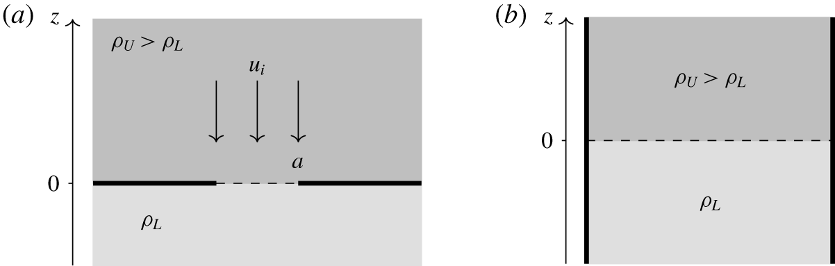
In this work we consider the vertical transfer of fluid through a horizontal opening, of area  $a$, between two miscible, incompressible fluids of different density (figure 1a). The opening provides the only connection between the fluids, which are otherwise separated by the horizontal plane at
 $z=0$. The fluid above the plane of the opening
 $(z>0)$, of density
 $\unicode[STIX]{x1D70C}_{U}$, is denser than the fluid below
 $(z<0)$, of density
 $\unicode[STIX]{x1D70C}_{L}$. Our focus is restricted to fluids with relatively small density differences so that the Boussinesq approximation (Boussinesq Reference Boussinesq1903) holds. Accordingly, with
 $g$ denoting the acceleration due to gravity, we define the reduced gravity of the system as
 $g^{\prime }=g(\unicode[STIX]{x1D70C}_{U}-\unicode[STIX]{x1D70C}_{L})/\unicode[STIX]{x1D70C}_{L}$ and acknowledge that
 $\unicode[STIX]{x1D70C}_{U}$ could instead be used as the reference density. The position of the interface between the two fluids,
 $z=\unicode[STIX]{x1D702}$, relative to the horizontal plane of the opening at
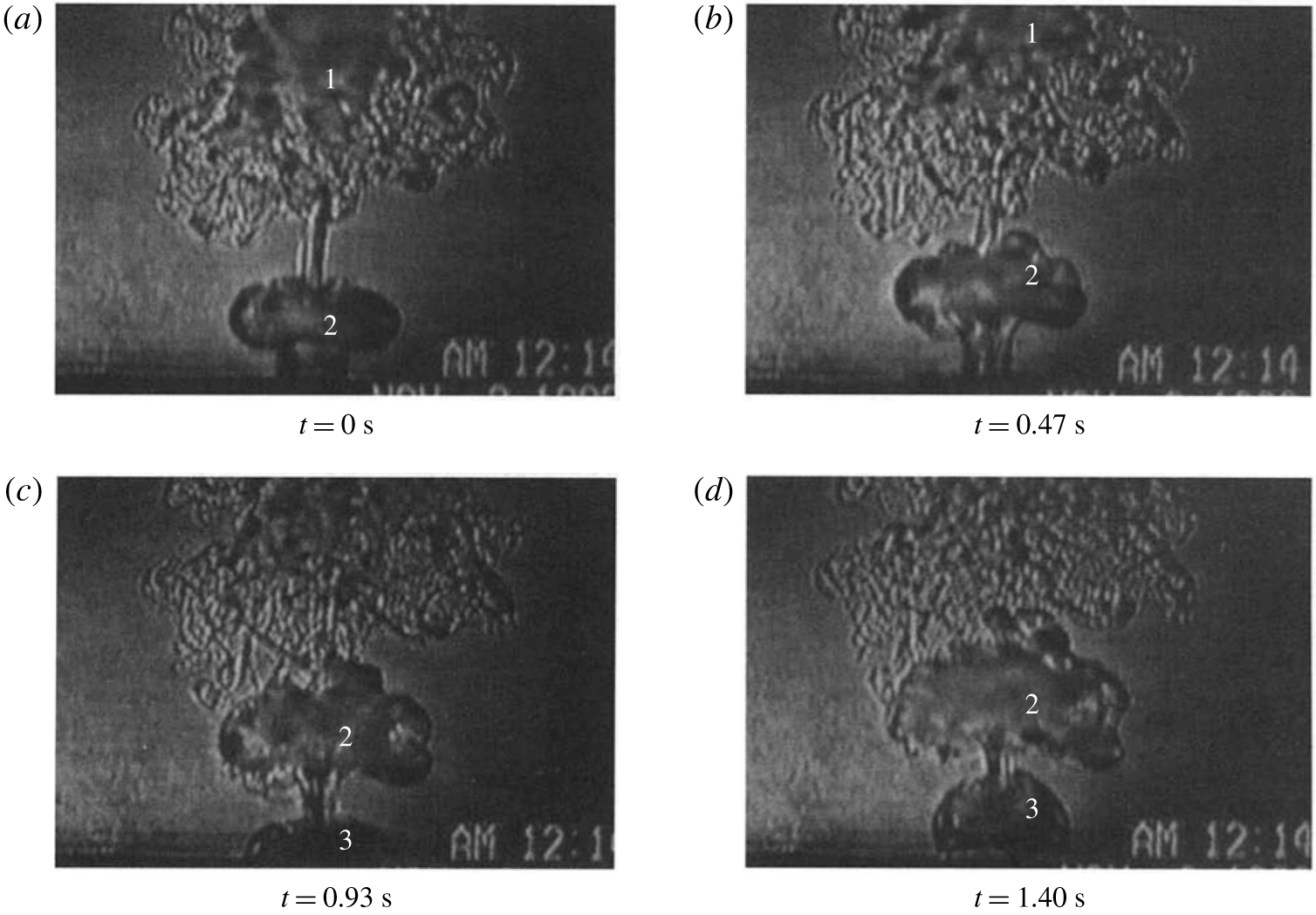
 $z=0$, is a function of the shape of the opening and time, and the initial perturbation. The amplitude of the perturbations will increase with time until the interface is so distorted that volumes of fluid are ‘pinched off’ and are thereby exchanged across the opening. The process of pinch off has been described in detail and illustrated by a time series of shadowgraph images by Conover, Kumar & Kapat (Reference Conover, Kumar and Kapat1995). These images have been reproduced in figure 2 to clarify what is observed in practice.
Schematics of the problems considered in this work (a) and by Sweeney, Kerswell & Mullin (Reference Sweeney, Kerswell and Mullin2013) (b). Fluid of density  $\unicode[STIX]{x1D70C}_{U}$ rests above fluid of density
 $\unicode[STIX]{x1D70C}_{L}<\unicode[STIX]{x1D70C}_{U}$. The undisturbed position of the interface between the lighter and heavier fluids is shown as a dashed line. In (a), an imposed flow of uniform speed
 $u_{i}$ advects the heavier fluid through the opening in the negative
 $z$ direction. (a) An opening of area
 $a$ in the horizontal plane
 $z=0$ separates the fluids. (b) An infinite vertical cylinder.

Time series of shadowgraph images of a pinch-off event during balanced exchange flow from Conover et al. (Reference Conover, Kumar and Kapat1995). The base of each image corresponds approximately to the plane of the opening. In (a) one can see the remnants of the previous pinch-off event (1) and the coherent structure associated with the current pinch-off event below (2). As the time series progresses, (1) and (2) rise and the next pinch-off structure (3) forms and starts to rise. Reproduced with permission from the Journal of Heat Transfer.

Exchange flows are triggered by the instability of an interface between a light fluid situated below a heavier fluid. This, the Rayleigh–Taylor instability, has been studied extensively (Taylor Reference Taylor1950; Bellman & Pennington Reference Bellman and Pennington1954; Dalziel, Linden & Youngs Reference Dalziel, Linden and Youngs1999; Wilkinson & Jacobs Reference Wilkinson and Jacobs2007). A linear stability analysis shows that perturbations on the interface grow exponentially at first (Chandrasekhar Reference Chandrasekhar1961), with the fastest growing mode corresponding to the wavenumber  $k\sim (g^{\prime }/\unicode[STIX]{x1D708}^{2})^{1/3}$, where
 $\unicode[STIX]{x1D708}$ is the average kinematic viscosity of the upper and lower fluids. After the initial exponential growth period, the linear modes saturate and nonlinear modes dominate with a quadratic growth rate (Youngs Reference Youngs1984), forming fingers of fluid that extend from the lower layer to the upper and vice versa. The fastest growing nonlinear mode is ultimately the largest that will fit in the opening. At this stage for the applications of interest, the scales are sufficiently large that the effects of viscosity are no longer important. Once the fingers reach a certain amplitude, they pinch off (figure 2). In this manner, fluid is transferred across the opening and an exchange flow established. In the approach we develop herein, the Rayleigh–Taylor mechanism enables us to identify the volume of light fluid that has crossed the plane of the opening in a given time. The physical details of how this volume pinches off to ultimately form a thermal-like coherent structure are not considered and are evidently complex (figure 2). We assume that after a characteristic time (calculated in § 4) a new event commences, entirely independent of the former, and there is no cross contamination (i.e. fluid that passes through the opening is not subsequently carried back through).
For the case of an infinite vertical cylinder, with light fluid below  $z=0$ and heavy fluid above, figure 1(b), there is an analytical solution for the linear instability of the interface in the inviscid limit (Maxwell Reference Maxwell2011). In the general viscous case, the equations for the growth rates and mode shapes require numerical solution (Sweeney et al. Reference Sweeney, Kerswell and Mullin2013). Similarly, we have been unable to find an analytical solution to the inviscid problem of interest here, namely to an interface initially in the plane of an opening made in an infinite horizontal plane. This solution remains elusive (appendix A).
As a consequence of the lack of an analytical solution for the time-varying position of an unstable interface in an opening in an infinite plane, previous theoretical work on balanced exchange flow (e.g. by Epstein (Reference Epstein1988)) is approximate and does not match some of the boundary conditions that define the physical problem. In extending the work of Epstein (Reference Epstein1988) to unbalanced exchange, we acknowledge that the solution we develop is approximate, however we note the excellent agreement (§ 8) with all the available experimental data.
Exchange flows occur in many different situations, including nuclear engineering (Kuhn et al. Reference Kuhn, Bernardis, Lee and Peterson2001), geophysics (Hughes et al. Reference Hughes, Bingham, Roussenov, Williams and Woodworth2015), building ventilation (Hunt & Coffey Reference Hunt and Coffey2010) and hydraulic engineering (Wilkinson Reference Wilkinson1988). There are theoretical models for predicting the volume flow rates associated with balanced exchange flow (Epstein Reference Epstein1988). Prior to the developments made herein, however, there was no theoretical model for an unbalanced exchange flow. This, and the numerous applications in which these unbalanced flows may occur, provided the primary motivation for this study. With these relatively large-scale environmental applications in mind, we shall not concern ourselves with problems in which interfacial tensions play a role and for the high Reynolds number flows of interest, focus on inviscid flows. Herein, we derive a mathematical model for predicting the volume flux of unbalanced exchange flows across thin-walled horizontal openings and compare the results to existing experimental data.
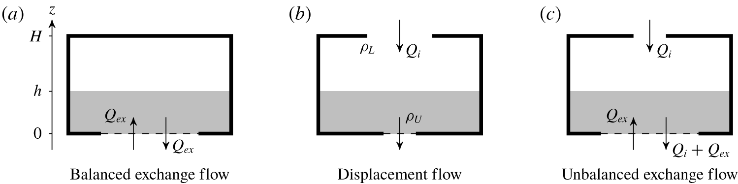
Schematics of different buoyancy-driven flows in emptying boxes with base and top openings. The box is surrounded by fluid of density  $\unicode[STIX]{x1D70C}_{L}$ and partially filled with negatively buoyant fluid of density
 $\unicode[STIX]{x1D70C}_{U}$.
 $Q_{i}$ and
 $Q_{ex}$ are the exchange and imposed volume fluxes, respectively.

Additional motivation for our work stems from a contradiction of the predictions of balanced exchange and displacement (or unidirectional) flow theory. This contradiction is best understood in the context of a naturally ventilated box, cf. the emptying box (Hunt & Coffey Reference Hunt and Coffey2010) and emptying–filling box (Linden, Lane-Serff & Smeed Reference Linden, Lane-Serff and Smeed1990). Balanced exchange flow theory predicts that for a box of negatively buoyant fluid relative to its surroundings, with a single horizontal opening in the base, there will be flow due to the Rayleigh–Taylor instability (figure 3a). By contrast, displacement flow theory (Linden et al. Reference Linden, Lane-Serff and Smeed1990) which, in general, considers a box with both top and base openings (figure 3b), predicts there will be no flow out of the box with the aforementioned geometry (i.e. zero flow rate in the limit as the area of the base opening tends to zero). In experimental work, Hunt & Coffey (Reference Hunt and Coffey2010) observed a flow pattern not accounted for by either balanced exchange flow or displacement flow theories. When the base opening was more than about four times larger than the top opening, Hunt & Coffey (Reference Hunt and Coffey2010) observed inflow through the top opening, as predicted by displacement flow theory, but both inflow and outflow simultaneously through the base opening (figure 3c). The flow out through the base opening must necessarily be greater in magnitude than the flow in through the base opening in order to conserve volume for the whole box. This phenomenon, the buoyancy-driven exchange of fluid across an opening against an imposed bulk flow, we refer to as unbalanced exchange flow. Shadowgraph images (§ 6) taken by Hunt & Coffey (Reference Hunt and Coffey2010) show that the pinch-off process identified for balanced exchange (Conover et al. Reference Conover, Kumar and Kapat1995, figure 2) also underlies unbalanced exchange. Our model of unbalanced exchange flow developed herein (§ 6) successfully overcomes this contradiction and, as such, bridges the gap between the unidirectional (idealised displacement) flow theory of Linden et al. (Reference Linden, Lane-Serff and Smeed1990) and the balanced exchange flow theory of Epstein (Reference Epstein1988). We place no restrictions herein on the mechanism responsible for creating the imposed bulk flow, e.g. it could be buoyancy driven or instead be mechanically driven, and so we are able to explore applications (§ 9) of our model beyond the context of a naturally ventilated box.
Regarding notation, we refer throughout to the volume flow rates, vertical velocity and dimensionless flow rates as  $Q$,
 $u$ and
 $Fr$ respectively, with the subscripts
 $(\cdot )_{ex}$,
 $(\cdot )_{i}$ and
 $(\cdot )_{i_{C}}$ referring respectively to exchange flow, imposed flow and critical values thereof. Initial conditions are designated by the subscript
 $(\cdot )_{0}$ and conditions at pinch off by the subscript
 $(\cdot )_{{\mathcal{P}}}$.
The remainder of this paper is structured as follows. Section 2 develops a physical reasoning for the scaling of the volume flux exchanged. Section 3 introduces a general condition for exchange flow that is valid for both balanced and unbalanced cases. To begin with, we focus on a circular opening. Section 4 considers the special limiting case of balanced exchange flow. Section 5 uses the condition introduced in § 3 to predict the transition from unidirectional to unbalanced exchange flow and comparisons are then made with the empirical value found by Hunt & Coffey (Reference Hunt and Coffey2010). In § 6 the method is extended to predict the volume flux for unbalanced exchange flows. Section 7 extends the analysis to a square opening. The theories developed for circular and square openings are compared to experimental data in § 8. Section 9 considers a few potential applications of the theory, with conclusions drawn in § 10.
2 Governing parameter and scaling for exchange volume flux
Although on dimensional grounds  $Q\sim a^{5/4}g^{\prime 1/2}$ is the only scaling possible for the volume flux exchanged, we first seek a physical reasoning that underlies this. Physically, the ‘unbalanced-ness’ of an unbalanced exchange flow is set by the growth rate of instabilities on the density interface in the plane of the opening relative to the rate at which fluid is advected through this opening by the imposed flow. This suggests that we may consider the relative time scales associated with these two components.
For exponentially growing modes with a time dependence of the form  $\text{e}^{nt}$ (see (4.3) and (7.1)), the time scale associated with the growth rate of instabilities is
 $$\begin{eqnarray}\unicode[STIX]{x1D70F}_{ins}=\frac{1}{n}.\end{eqnarray}$$
The time scale associated with advection by the steady imposed flow  $Q_{i}\propto au_{i}$ (figure 1a) is
 $$\begin{eqnarray}\unicode[STIX]{x1D70F}_{adv}=\frac{{\mathcal{L}}}{u_{i}}\propto \frac{{\mathcal{L}}a}{Q_{i}},\end{eqnarray}$$
where  ${\mathcal{L}}$ is a characteristic vertical length scale. Therefore, for a general (circular, square, etc.) opening, we may write
 $$\begin{eqnarray}\frac{\unicode[STIX]{x1D70F}_{ins}}{\unicode[STIX]{x1D70F}_{adv}}=\frac{Q_{i}}{{\mathcal{L}}an}.\end{eqnarray}$$
As we shall see in § 4, for a circular opening of diameter  $D$,
 $n=(kg^{\prime }/2)^{1/2}$ with
 $k$ the radial wavenumber and volume conservation requires
 $kD=\text{const.}$ (§ 4). Therefore,
 $$\begin{eqnarray}\unicode[STIX]{x1D70F}_{ins}=\left(\frac{2}{kg^{\prime }}\right)^{1/2}=\left(\frac{2D}{kDg^{\prime }}\right)^{1/2}\propto \left(\frac{D}{g^{\prime }}\right)^{1/2},\end{eqnarray}$$
and the time scale for the growth of instabilities scales only on opening diameter and reduced gravity. Thus, with  ${\mathcal{L}}=D$ and writing
 $a=\unicode[STIX]{x03C0}D^{2}/4$ gives
 $$\begin{eqnarray}\frac{\unicode[STIX]{x1D70F}_{ins}}{\unicode[STIX]{x1D70F}_{adv}}\propto \frac{Q_{i}}{D^{3}}\left(\frac{D}{g^{\prime }}\right)^{1/2}=\frac{Q_{i}}{D^{5/2}g^{\prime 1/2}},\end{eqnarray}$$
or
 $$\begin{eqnarray}\frac{\unicode[STIX]{x1D70F}_{ins}}{\unicode[STIX]{x1D70F}_{adv}}\propto \frac{Q_{i}}{a^{5/4}g^{\prime 1/2}}=Fr_{i}.\end{eqnarray}$$
In other words, this ratio naturally gives rise to the exchange volume flow rate scaling  $a^{5/4}g^{\prime 1/2}$ and means that the dimensionless flow rate
 $Fr_{i}$ is proportional to the ratio of time scales for instability growth and imposed flow advection. If we treat
 $Fr_{i}$ as a parameter, then (2.6) shows that varying this parameter alters the ratio of time scales and thereby alters the exchange through the opening.
3 A general condition for exchange flow
Consider an imposed unidirectional downflow of uniform speed  $u_{i}=Q_{i}/ac_{d}$ through the opening. Here,
 $c_{d}\,({<}1)$ denotes the loss coefficient associated with the opening (e.g. Ward-Smith Reference Ward-Smith1980). As a first approximation, it may be assumed that the imposed flow advects the interface such that, moving in a frame of reference with the interface, perturbations grow as if there were no imposed flow. This is a reasonable approximation for high Reynolds number flow through an opening as the velocity profile is then well approximated as uniform (Lamb Reference Lamb1932; Etheridge & Sandberg Reference Etheridge and Sandberg1996). If we denote
 $\unicode[STIX]{x1D702}_{{\mathcal{P}}}$ as the displacement of the interface at pinch off,
 $t_{{\mathcal{P}}}$ as the time taken for the perturbation to grow to pinch off and
 $s_{{\mathcal{P}}}=u_{i}t_{{\mathcal{P}}}$ as the vertical distance that the perturbation is advected downwards by the imposed flow in a time
 $t_{{\mathcal{P}}}$, then the condition for exchange flow to occur, whether balanced (§ 4) or unbalanced (§ 5), can then be stated as
 $$\begin{eqnarray}\unicode[STIX]{x1D702}_{{\mathcal{P}},max}-\unicode[STIX]{x1D702}_{0,max}>s_{{\mathcal{P}}},\end{eqnarray}$$
where  $\unicode[STIX]{x1D702}_{{\mathcal{P}},max}=\text{max}\{|\unicode[STIX]{x1D702}(t=t_{{\mathcal{P}}})|\}$ and
 $\unicode[STIX]{x1D702}_{0,max}=\text{max}\{|\unicode[STIX]{x1D702}(t=0)|\}$. We restrict our attention to steady imposed flows so that
 $u_{i}$ does not vary in the interval from
 $t=0$ to
 $t=t_{{\mathcal{P}}}$. The inequality (3.1) is a general condition which makes no assumptions about the form of the perturbation or the mechanism driving the imposed flow. With reference to § 2, equation (3.1) can be rewritten as
 $$\begin{eqnarray}\frac{\unicode[STIX]{x1D702}_{{\mathcal{P}},max}-\unicode[STIX]{x1D702}_{0,max}}{a^{1/2}}\propto Fr_{i},\end{eqnarray}$$
with the governing parameter  $Fr_{i}$ thereby expressed as a ratio of the vertical and horizontal length scales of the exchange flow.
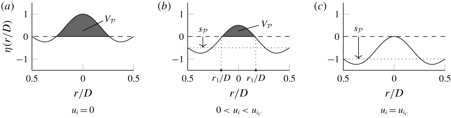
The possible flow regimes resulting from (3.1) are shown schematically in figures 4(a) and 4(b), where the instability for circular openings is considered simply for convenience. The figure shows the interface position  $\unicode[STIX]{x1D702}$ with radial coordinate
 $r$ for a mode of interest (§ 4), the coordinate origin located at the centre of the opening. Balanced exchange flow occurs when the imposed flow velocity is zero (figure 4a), i.e.
 $Q_{i}\equiv 0$ and thereby
 $Fr_{i}\equiv 0$, so that
 $s_{{\mathcal{P}}}\equiv 0$. With a sufficiently large imposed flow velocity, corresponding to
 $u_{i}>u_{i_{C}}$, any perturbation on the density interface would be advected downwards so that there is unidirectional downflow, i.e. no exchange can occur. Figure 4(c) shows the critical case where
 $u_{i}=u_{i_{C}}$ so that the entire perturbation is just advected across the plane of the opening and flow is again unidirectional downflow albeit with at least one location with zero velocity in the plane of the opening. For
 $0<u_{i}<u_{i_{C}}$ the perturbation will grow fast enough such that it is not completely advected across the plane of the opening at pinch off (figure 4b). This is an unbalanced exchange flow and is characterised by a greater volume of the perturbation below the plane of the opening than the volume
 $V_{{\mathcal{P}}}$ above (shown shaded) when the perturbation has been advected downwards by a distance
 $s_{{\mathcal{P}}}$. For the critical imposed flow in figure 4(c),
 $V_{{\mathcal{P}}}=0$.
Vertical sections through the perturbation at  $t=t_{{\mathcal{P}}}$ for different downwards imposed flow velocities. (a) Zero velocity, corresponding to balanced exchange flow; the areas shown in the section are not equal, however upon rotation about
 $r=0$ the swept out volumes above,
 $V_{{\mathcal{P}}}$, (shaded grey) and below the plane of the opening (dashed line) are equal. (b) Unbalanced exchange flow – the imposed velocity is too weak to advect the perturbation completely across the plane of the opening. (c) The critical case where there is no exchange (
 $V_{{\mathcal{P}}}=0$) and flow is unidirectional in the plane of the opening.

4 Balanced exchange flow
We consider now the general condition (3.1) with  $u_{i}\equiv 0$. In this case, the condition is met for any growing perturbation unless
 $\unicode[STIX]{x1D702}_{{\mathcal{P}},max}=\unicode[STIX]{x1D702}_{0,max}$, i.e. unless the system is stable so there is no change in the magnitude of the perturbations with time.
For openings with thin walls  $(L/D\ll 1)$, there is almost no pressure difference across the opening and, therefore, one would expect no flow in the limit as the wall thickness
 $L\rightarrow 0$. However, as shown by Taylor (Reference Taylor1950), the interface is unstable to any disturbance.
As mentioned in § 1 and discussed in appendix A, there is not currently an analytical solution for the position and growth of an interface at an opening in an infinite plane separating two fluids of different density. Therefore, any description of the interface position is necessarily approximate. In the inviscid limit, the expected form of the perturbation for the vertical velocity,  $u(r,\unicode[STIX]{x1D703},z=0)$, in cylindrical polar coordinates (i.e. taking the inviscid limit of (A 2) at
 $z=0$) is
 $$\begin{eqnarray}u(r,\unicode[STIX]{x1D703},z=0)=A\text{J}_{m}(kr)\text{e}^{\text{i}m\unicode[STIX]{x1D703}+nt},\end{eqnarray}$$
where  $A$ is a constant,
 $\text{J}_{m}$ is the Bessel function of the first kind of order
 $m$ and
 $m$ is the azimuthal wavenumber. Whilst one might anticipate that the flow toward the opening is irrotational and the flow away is not, as a first approximation we treat the entire flow local to the opening as irrotational. Based on the observations and measurements of Conover et al. (Reference Conover, Kumar and Kapat1995) and Varrall et al. (Reference Varrall, Pretrel, Vaux and Vauquelin2016) we assume that the flow is axisymmetric, i.e.
 $m=0$. The interface position is, therefore,
 $$\begin{eqnarray}\unicode[STIX]{x1D702}=\hat{\unicode[STIX]{x1D702}}\text{J}_{0}(kr)\text{e}^{nt},\end{eqnarray}$$
where the constant  $\hat{\unicode[STIX]{x1D702}}$ is the amplitude of the perturbation at
 $t=0$. Although we consider an infinitesimally thin-walled opening, any real opening will have a finite thickness and, therefore, a no-slip condition on the perimeter at
 $r=D/2$. This assertion is supported by the experimental measurement of velocity profiles in balanced exchange flow (with characteristic Reynolds number
 $Re\sim 500$) by Varrall et al. (Reference Varrall, Pretrel, Vaux and Vauquelin2016) who observed zero velocity at the perimeters of their circular openings. The only way of ensuring zero velocity at the perimeter for (4.2) is by selecting a value of
 $k$ such that
 $\text{J}_{0}(kD/2)=0$. However, volume is not conserved for all values of
 $k$ satisfying
 $\text{J}_{0}(kD/2)=0$ as we impose
 $\unicode[STIX]{x1D702}=0$ for
 $r>D/2$ (no fluid can pass through the horizontal plane). Therefore, following Epstein (Reference Epstein1988), we modify (4.2) to be
 $$\begin{eqnarray}\unicode[STIX]{x1D702}=\hat{\unicode[STIX]{x1D702}}[\text{J}_{0}(kr)-\text{J}_{0}(kD/2)]\text{e}^{nt}.\end{eqnarray}$$
Whilst not an exact solution for the interface position, equation (4.3) has the convenient property that  $\unicode[STIX]{x1D702}(D/2,t)\equiv 0\,\forall \,k$. This means we can select a value of
 $k$ that allows for conservation of volume. When dealing with the unbalanced exchange case (§ 6) we relax the requirement of no slip and allow the profile (figure 4a) to be advected by a uniform velocity (figure 4b,c). The assumption of a uniform velocity profile is routinely made for high
 $Re$ flow and the good agreement of the resulting predictions with experimental data (§ 8) provides justification for this simplified approach.
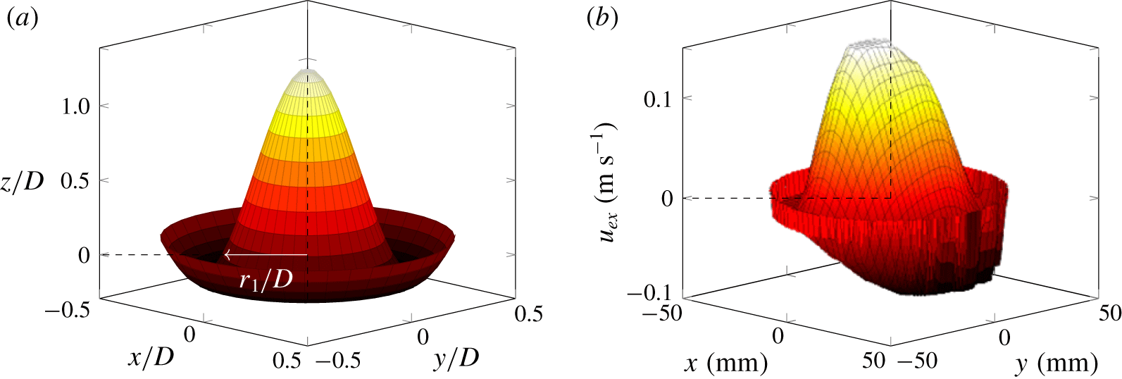
The perturbation (4.3) consists of a central rising fluid core surrounded by a descending outer annulus, as shown in figure 5(a). This form is consistent with the experimental results of Varrall et al. (Reference Varrall, Pretrel, Vaux and Vauquelin2016), adapted in figure 5(b), who observed and measured balanced exchange flow through a circular opening using stereoscopic particle image velocimetry (PIV). The theoretical and experimental profiles show similar features, such as a rising central region and a descending outer annulus. For Boussinesq flow there is no physical reason why the profile should have a preferred orientation, however both the works of Varrall et al. (Reference Varrall, Pretrel, Vaux and Vauquelin2016) and Conover et al. (Reference Conover, Kumar and Kapat1995) show the less dense finger of fluid rising through the centre of the opening and the denser fluid falling through the outer annular region. We offer no explanation for why this is the case although, with reference to figure 4, acknowledge that the critical velocity of the imposed flow will vary with orientation. Indeed our approach would suggest that if there were to be a ‘finger out’ of dense fluid, with reference to figure 4, the amplitude of the annular perimeter of light fluid at time  $t_{{\mathcal{P}}}$ relative to the distance advected by the imposed flow would be relevant. Given the annulus protrudes less far than the tip of the finger, the volume flux exchanged would be lower for the ‘finger out’ orientation for a given imposed flow – i.e. the exchange would be weaker – and the critical value at which the unbalanced exchange flow were reduced to zero (cf. § 5) would, similarly, be reduced. The measured profile (figure 5b) is not fully axisymmetric, with a varying velocity around the annulus. It may be that if a greater time-averaging period were used, the flow would converge to axisymmetry.
The Boussinesq approximation implies that conservation of mass for the exchange flow is equivalent to conservation of volume for the small density differences considered herein. Conservation of volume for the (rising) central finger and the (descending) outer annulus requires  $kD$ to satisfy
 $$\begin{eqnarray}\text{J}_{1}(kD/2)=\frac{kD\text{J}_{0}(kD/2)}{4},\end{eqnarray}$$
for which  $kD=\hat{k}=\text{const.}=10.27$ (to 2 decimal places (d.p.)) is the smallest positive, non-trivial root (appendix B). This level of precision is necessary to give a difference of 1 % in the volumes of the finger and annulus. Here we have taken the dominant nonlinear wavenumber, i.e. the mode with the largest wavelength that will fit into the opening, in combination with the linear exponential growth rate for simplicity. Although simplified, it will be seen that the analysis that stems from this form leads to compelling results.
Comparison of the theoretical form of the perturbation considered at  $t=t_{{\mathcal{P}}}$ with a time-averaged velocity profile from Varrall et al. (Reference Varrall, Pretrel, Vaux and Vauquelin2016), where
 $u_{ex}$ is the vertical perturbation velocity. The plane of the opening is at
 $z/D=0$. (a) Circular opening perturbation (4.3). (b) Time-averaged velocity profile from Varrall et al. (Reference Varrall, Pretrel, Vaux and Vauquelin2016).

Epstein (Reference Epstein1988) assumed that the fingers of fluid pinched off when they had reached a height of  $O(D)$. This assumption was supported by his visual observations. Setting
 $\unicode[STIX]{x1D702}=D$ on
 $r=0$ in (4.3) and noting that
 $\text{J}_{0}(0)=1$ gives the time to pinch off as
 $$\begin{eqnarray}t_{{\mathcal{P}}}=\frac{1}{n}\ln \left(\frac{D}{(1-\text{J}_{0}(\hat{k}/2))\hat{\unicode[STIX]{x1D702}}}\right)=\left(\frac{2}{\hat{k}}\right)^{1/2}\left(\frac{D}{g^{\prime }}\right)^{1/2}\ln \left(\frac{D}{c\hat{\unicode[STIX]{x1D702}}}\right),\end{eqnarray}$$
with  $c=1-\text{J}_{0}(\hat{k}/2)\approx 1.13$. Evidently, this time scale increases as the opening diameter increases and decreases as the density step across the opening increases.
Given  $\text{d}(\text{J}_{0}(kr))/\text{d}r=-k\text{J}_{1}(kr)$, where
 $\text{J}_{1}$ is the Bessel function of the first kind of order one, the volume of the finger at pinch off,
 $V_{{\mathcal{P}}}$, (figure 4a) is given by
 $$\begin{eqnarray}V_{{\mathcal{P}}}=\int _{0}^{\unicode[STIX]{x1D702}_{{\mathcal{P}}}}\unicode[STIX]{x03C0}r^{2}\,\text{d}\unicode[STIX]{x1D702}=\frac{\unicode[STIX]{x03C0}\hat{k}}{c}\int _{0}^{r_{1}}r^{2}\,\text{J}_{1}\left(\frac{\hat{k}r}{D}\right)\text{d}r\approx 0.088D^{3},\end{eqnarray}$$
where  $r_{1}\approx 0.26D$ is the radius of the finger in the plane of the opening (figure 5a). Note that the pinch-off volume is independent of the initial form of the disturbance (i.e. that given in (4.3) at
 $t=0$), but that the initial form affects the time taken to pinch off and thereby the volume flux exchanged.
Using (4.5) and (4.6) the volume flux associated with each pinch-off event,  $Q_{{\mathcal{P}}}$, can now be estimated as
 $$\begin{eqnarray}Q_{{\mathcal{P}}}=\frac{V_{{\mathcal{P}}}}{t_{{\mathcal{P}}}}\approx \frac{0.20}{\ln \left({\displaystyle \frac{D}{c\hat{\unicode[STIX]{x1D702}}}}\right)}(D^{5}g^{\prime })^{1/2}.\end{eqnarray}$$
In practice, the volume flux exchanged at a given instant will not be as (4.7) due to random fluctuations. However, the average over long times,  $Q_{ex_{B}}$, is expected to converge to
 $Q_{{\mathcal{P}}}$. The experimental work of Varrall et al. (Reference Varrall, Pretrel, Vaux and Vauquelin2017) suggests that an averaging period of
 $T>3000\;t_{{\mathcal{P}}}$ is required for
 $Q_{ex_{B}}$ to converge. Accordingly, we take
 $$\begin{eqnarray}Q_{ex_{B}}=Q_{{\mathcal{P}}}.\end{eqnarray}$$
In order to evaluate (4.7) we must assign a value to  $\ln (D/\hat{\unicode[STIX]{x1D702}})$. Conover et al. (Reference Conover, Kumar and Kapat1995) investigated the behaviour of balanced exchange flow through a thin-walled horizontal opening using laser Doppler velocimetry. They found that the flow pulsated across the opening at a frequency dependent on the opening aspect ratio
 $L/D$. Assuming that the frequency measured is the inverse of the time to pinch off, their experimental values can be used to estimate
 $\ln (D/\hat{\unicode[STIX]{x1D702}})$. Epstein (Reference Epstein1988) cited Lewis (Reference Lewis1950) in taking
 $\ln (D/\hat{\unicode[STIX]{x1D702}})=5$ but was not explicit regarding where this value came from. The experiments of Lewis (Reference Lewis1950) showed that the fingers of fluid separated for
 $\text{cosh}(4)\lesssim \unicode[STIX]{x1D702}/\hat{\unicode[STIX]{x1D702}}\lesssim \text{cosh}(5)$, giving
 $3.3\lesssim \ln (D/\hat{\unicode[STIX]{x1D702}})\lesssim 4.3$. The hyperbolic cosine results from the formulation of the linear instability problem by Taylor (Reference Taylor1950) which Lewis (Reference Lewis1950) was testing. Lewis’s set-up is also different to that considered by Epstein (Reference Epstein1988), in that Lewis (Reference Lewis1950) considered fluid confined in a thin gap between two parallel plates so that the flow is quasi-two-dimensional as opposed to three-dimensional. It may be expected, therefore, that
 $\ln (D/\hat{\unicode[STIX]{x1D702}})$ could take a different value.
The opening with the smallest aspect ratio used by Conover et al. (Reference Conover, Kumar and Kapat1995) is  $L/D=0.008$ with a frequency of pinch-off events of 0.7 Hz, giving
 $t_{{\mathcal{P}}}=1.4~\text{s}$. Taking
 $D=0.0508~\text{m}$ and
 $g^{\prime }=0.118~\text{m}~\text{s}^{-2}$ directly from their experimental set-up, equation (4.5) gives
 $\ln (D/\hat{\unicode[STIX]{x1D702}})=5.1$ (to 2 significant figures (s.f.)), approximately the value used by Epstein (Reference Epstein1988). Rearranging gives
 $\hat{\unicode[STIX]{x1D702}}=\text{e}^{-5.1}D$, suggesting the initial amplitude of perturbation
 $\hat{\unicode[STIX]{x1D702}}\sim O(0.01D)$. This gives
 $$\begin{eqnarray}Fr_{ex_{B}}=\frac{Q_{ex_{B}}}{a^{5/4}g^{\prime 1/2}}=\frac{0.20\times 2^{5/2}}{\unicode[STIX]{x03C0}^{5/4}\ln \left({\displaystyle \frac{D}{c\hat{\unicode[STIX]{x1D702}}}}\right)}\approx 0.055.\end{eqnarray}$$
This is the balanced exchange flow limit of (3.1) achieved when  $u_{i}=0$ so that
 $s_{{\mathcal{P}}}\equiv 0$.
Epstein (Reference Epstein1988) expressed the dimensionless volume flux exchanged as a Froude number,  $Fr_{Eps}=Q_{ex_{B}}/(D^{5}g^{\prime })^{1/2}$, the subscript
 $(\cdot )_{Eps}$ used here to distinguish Epstein’s (Reference Epstein1988) definition, based on the opening diameter, from that used herein based on the opening area across which fluid exchanges. The two definitions are related by
 $$\begin{eqnarray}Fr_{Eps}=\frac{\unicode[STIX]{x03C0}^{5/4}}{2^{5/2}}Fr_{ex_{B}},\end{eqnarray}$$
which, with (4.9), gives  $Fr_{Eps}=0.041$. The use of opening area in the definition of Froude number instead of diameter permits comparison with the measurements of Hunt & Coffey (Reference Hunt and Coffey2010), see § 5, and allows the analysis of opening geometries other than circular (§ 7).
5 The onset of exchange flow
A second special case of (3.1) is equality, i.e.  $\unicode[STIX]{x1D702}_{{\mathcal{P}},max}-\unicode[STIX]{x1D702}_{0,max}=s_{{\mathcal{P}}}=u_{i}t_{{\mathcal{P}}}$. This is the condition for the initiation of unbalanced exchange flow, where the maximum displacement of the perturbation at pinch off is at the plane of the opening as depicted in figure 4(c).
The characteristic imposed velocity magnitude  $u_{i_{C}}$ corresponding to a critical imposed flow rate
 $Q_{i_{C}}$ down through the opening is
 $u_{i_{C}}=Q_{i_{C}}/ac_{d}$, so that (3.1) gives
 $$\begin{eqnarray}\unicode[STIX]{x1D702}_{{\mathcal{P}},max}-\unicode[STIX]{x1D702}_{0,max}=\frac{Q_{i_{C}}}{ac_{d}}t_{{\mathcal{P}}}.\end{eqnarray}$$
Substituting for  $t_{{\mathcal{P}}}$ from (4.5) with
 $\ln (D/c\hat{\unicode[STIX]{x1D702}})=4.9$ and
 $D^{2}=4a/\unicode[STIX]{x03C0}$ gives
 $$\begin{eqnarray}\frac{\unicode[STIX]{x1D702}_{{\mathcal{P}},max}-\unicode[STIX]{x1D702}_{0,max}}{D}=\frac{b}{c_{d}}Fr_{i_{C}},\end{eqnarray}$$
where  $Fr_{i_{C}}=Q_{i_{C}}/a^{5/4}g^{\prime 1/2}$ is the critical imposed dimensionless volume flux and
 $b=\unicode[STIX]{x03C0}^{1/4}\ln (D/c\hat{\unicode[STIX]{x1D702}})/\hat{k}^{1/2}$. We may neglect
 $\unicode[STIX]{x1D702}_{0,max}/D=O(10^{-2})$ and so rearranging for
 $Fr_{i_{C}}$, using (5.2) and
 $\unicode[STIX]{x1D702}_{{\mathcal{P}},max}=D$ gives the dimensionless imposed volume flux at the onset of exchange as
 $$\begin{eqnarray}Fr_{i_{C}}=\frac{c_{d}}{b}\approx 0.29.\end{eqnarray}$$
In (5.3) we have taken  $c_{d}=0.60$ as in Hunt & Coffey (Reference Hunt and Coffey2010) and as suggested by Ward-Smith (Reference Ward-Smith1980) and Etheridge & Sandberg (Reference Etheridge and Sandberg1996). This is valid within our assumption that unbalanced exchange flow through a horizontal opening can be modelled as the superposition of unidirectional flow through the opening and balanced exchange flow through the opening; for unidirectional flow through a sharp-edged orifice the loss coefficient is widely taken to be
 $c_{d}=0.6$.
If the assumption of superposition were not made, it is not known what value  $c_{d}$ would take, or indeed how it would be defined. For unidirectional flow through an orifice the greatest contribution to
 $c_{d}$ is from the vena contracta, however this phenomenon is not necessarily relevant to bidirectional flows. Another way of viewing
 $c_{d}$ is as the ratio of measured to theoretical volume flux, but taking the work on balanced exchange flow of Epstein (Reference Epstein1988) as an example, the theoretical volume flux is less than the measured, so that
 $c_{d}>1$. This is considered no further.
Our analysis leads to an estimate for  $Fr_{i_{C}}$ that agrees closely with the value that Hunt & Coffey (Reference Hunt and Coffey2010) deduced from their measurements, namely 0.33. They arrived at this value by a fit to their experimental data, not by prediction from theory. It is also worthy of note that, whilst Hunt & Coffey (Reference Hunt and Coffey2010) were considering an imposed volume flux due to a buoyancy-driven displacement flow, no assumptions about the mechanism driving the imposed flow have been made herein for the analysis leading to (5.3). With the measurements of Hunt & Coffey (Reference Hunt and Coffey2010) and our current analysis arriving independently at
 $Fr_{i_{C}}\approx 0.3$, we have confidence in the assertion that an imposed dimensionless volume flux falling much below this value will result in the onset of (unbalanced) exchange flow through a horizontal circular opening.
6 Unbalanced exchange flows
The method used to predict the balanced exchange flow in § 4 is readily extended to general non-zero background velocities  $0<u_{i}<u_{i_{C}}$ associated with an imposed flow by calculating the time to pinch off
 $t_{{\mathcal{P}}}$ and the volume
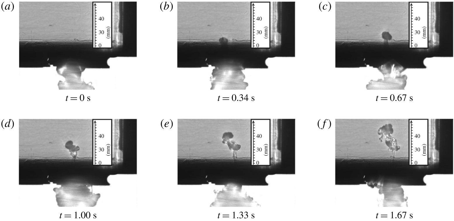
 $V_{{\mathcal{P}}}$ of the perturbation above the plane of the opening at pinch off (figure 4b). The validity of this approach is supported by the experiments of Hunt & Coffey (Reference Hunt and Coffey2010) who observed pinch-off events during unbalanced exchange flow (figure 6).
Time series of shadowgraph images of a pinch-off event during unbalanced exchange flow from the experiments of Hunt & Coffey (Reference Hunt and Coffey2010).

The position of the perturbed interface at pinch off is given by
 $$\begin{eqnarray}\unicode[STIX]{x1D702}_{{\mathcal{P}}}=\unicode[STIX]{x1D702}(r,t_{{\mathcal{P}}})=[\text{J}_{0}(\hat{k}r/D)-\text{J}_{0}(\hat{k}/2)]\frac{D}{c}-s_{{\mathcal{P}}}.\end{eqnarray}$$
Defining  $\unicode[STIX]{x1D702}_{{\mathcal{P}}}(r_{1})=0$ (figure 4b), equation (6.1) gives the equation for
 $r_{1}$ as
 $$\begin{eqnarray}\frac{s_{{\mathcal{P}}}}{D}=\frac{\text{J}_{0}(\hat{k}r_{1}/D)-\text{J}_{0}(\hat{k}/2)}{c}.\end{eqnarray}$$
Non-dimensionalising the imposed volume flux as indicated by the balanced exchange flow scaling, so that  $Fr_{i}=Q_{i}/(a^{5/4}g^{\prime 1/2})$, recalling that
 $s_{{\mathcal{P}}}=u_{i}t_{{\mathcal{P}}}$ and using (4.5), the distance the perturbation is advected can be expressed as
 $$\begin{eqnarray}\frac{s_{{\mathcal{P}}}}{D}=\frac{b}{c_{d}}Fr_{i}.\end{eqnarray}$$
Equating (6.2) and (6.3) gives the following implicit equation for  $r_{1}$ as a function of
 $Fr_{i}$
 $$\begin{eqnarray}\text{J}_{0}(\hat{k}r_{1}/D)=\text{J}_{0}(\hat{k}/2)+\frac{cb}{c_{d}}Fr_{i},\end{eqnarray}$$
which can be solved numerically. The solution is single valued for  $0<Fr_{i}<Fr_{i_{C}}$. The volume of fluid above the plane of the opening at
 $t=t_{{\mathcal{P}}}$ is given by
 $$\begin{eqnarray}V_{{\mathcal{P}}}=\int _{0}^{\unicode[STIX]{x1D702}_{{\mathcal{P}}}-s_{{\mathcal{P}}}}\unicode[STIX]{x03C0}r^{2}\,\text{d}\unicode[STIX]{x1D702}=\frac{\unicode[STIX]{x03C0}\hat{k}}{c}\int _{0}^{r_{1}}r^{2}\text{J}_{1}(\hat{k}r/D)\,\text{d}r=\frac{\unicode[STIX]{x03C0}Dr_{1}^{2}}{c}\text{J}_{2}(\hat{k}r_{1}/D),\end{eqnarray}$$
where  $\text{J}_{2}$ is the Bessel function of the first kind of order two. Therefore,
 $$\begin{eqnarray}Q_{ex}=Q_{{\mathcal{P}}}=\frac{V_{{\mathcal{P}}}}{t_{{\mathcal{P}}}}=\frac{\unicode[STIX]{x03C0}(\hat{k}/2)^{1/2}}{c\ln \left({\displaystyle \frac{D}{c\hat{\unicode[STIX]{x1D702}}}}\right)}r_{1}^{2}\text{J}_{2}(kr_{1})(Dg^{\prime })^{1/2},\end{eqnarray}$$
and
 $$\begin{eqnarray}Fr_{ex}=\frac{Q_{ex}}{a^{5/4}g^{\prime 1/2}}=\frac{4r_{1}^{2}}{D^{2}cb}\text{J}_{2}(\hat{k}r_{1}/D).\end{eqnarray}$$
Thus, for a given or imposed dimensionless flow rate through the opening  $Fr_{i}$, the strength
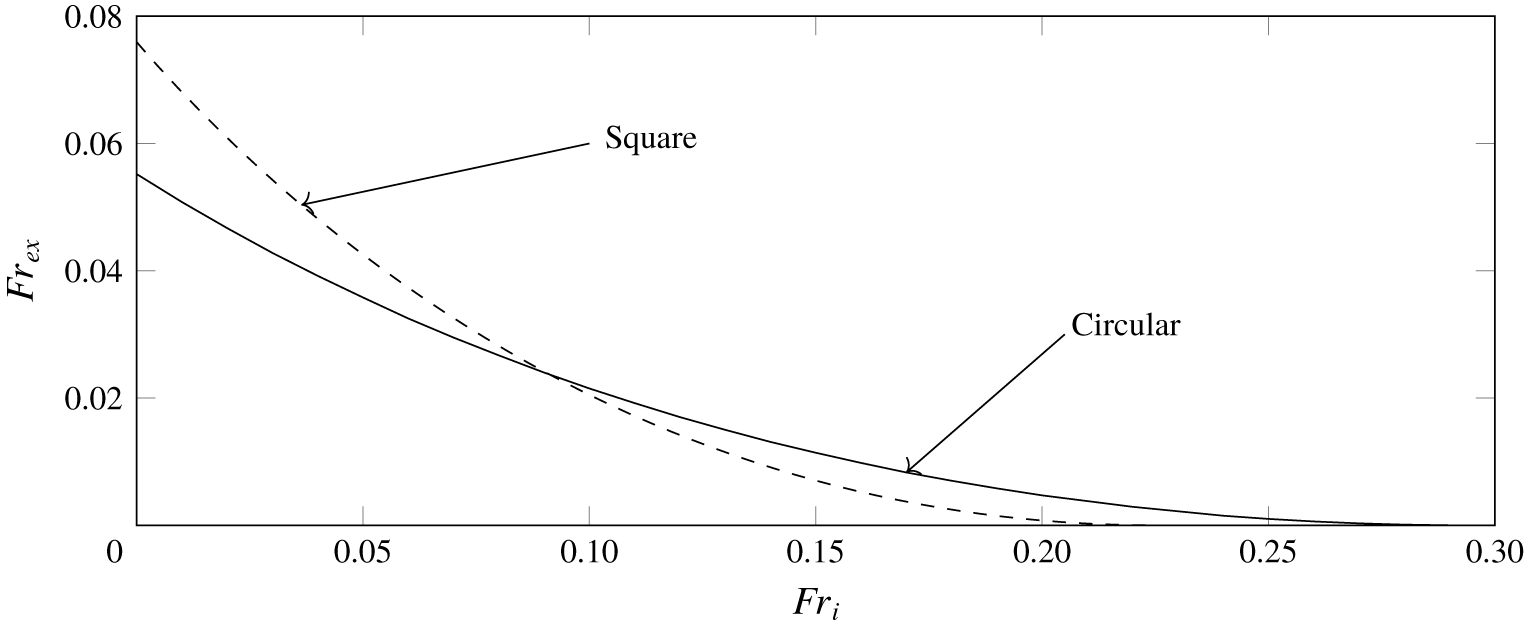
 $Fr_{ex}$ of the dimensionless volume flux exchanged can be calculated. Our predictions from (6.7) are plotted in figure 7 (solid line). The variation of
 $Fr_{ex}$ with
 $Fr_{i}$ is smooth and monotonically decreasing, as would be expected. In other words, the stronger the imposed flow, the weaker the exchange, until with
 $Fr_{i}=0.29$ (to 2 s.f.) the exchange flow rate is reduced to zero. The contribution to the total flow from exchange is insignificant relative to the imposed flow even at
 $Fr_{i}\sim 0.1$. Only at
 $Fr_{i}=0.039$ (to 2 s.f.) are the contributions equal.


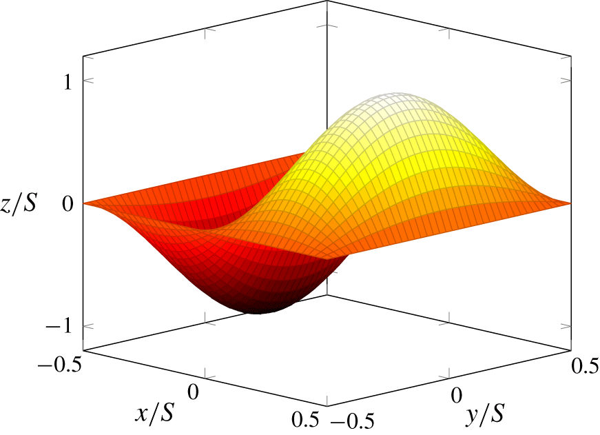
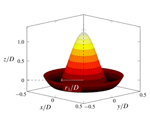
Square opening perturbation  $z=\unicode[STIX]{x1D702}$ from (7.1) plotted at
 $t=t_{{\mathcal{P}}}$.

7 Other geometries
Epstein (Reference Epstein1988) and Hunt & Coffey (Reference Hunt and Coffey2010) considered circular openings, however the analysis in §§ 4–6 can be readily applied to other opening shapes provided there are analytical solutions to waves on an interface bounded by that shape. There is no analytical solution for waves on an interface with an arbitrary boundary but there is for waves with a rectangular boundary.
We now consider the case of a square opening with sides of length  $S$. The mode with the lowest wavenumbers in
 $x$ and
 $y$ such that volume is conserved is
 $$\begin{eqnarray}\unicode[STIX]{x1D702}=\hat{\unicode[STIX]{x1D702}}\text{e}^{nt}\sin (2\unicode[STIX]{x03C0}x/S)\sin (\unicode[STIX]{x03C0}y/S),\end{eqnarray}$$
which is plotted in figure 8. The composite wavenumber  $k=(k_{x}^{2}+k_{y}^{2})^{1/2}$, for horizontal components
 $k_{x}$ and
 $k_{y}$, and so
 $n=(kg^{\prime }/2)^{1/2}$ and (7.1) give
 $$\begin{eqnarray}k=\frac{5^{1/2}\unicode[STIX]{x03C0}}{S},\quad n=\left(\frac{5^{1/2}\unicode[STIX]{x03C0}g^{\prime }}{2S}\right)^{1/2},\quad t_{{\mathcal{P}}}=\left(\frac{2S}{5^{1/2}\unicode[STIX]{x03C0}g^{\prime }}\right)^{1/2}\ln \left(\frac{S}{\hat{\unicode[STIX]{x1D702}}}\right).\end{eqnarray}$$
As before, § 4, we take  $\ln (S/\hat{\unicode[STIX]{x1D702}})=5$, where the logarithm again results from the assumed exponential growth of the interface. At
 $t=t_{{\mathcal{P}}}$,
 $\unicode[STIX]{x1D702}_{{\mathcal{P}},max}=S$ and with reference to figure 8,
 $$\begin{eqnarray}V_{{\mathcal{P}}}=\int _{0}^{S}\int _{0}^{S/2}\unicode[STIX]{x1D702}\,\text{d}x\,\text{d}y=\frac{2}{\unicode[STIX]{x03C0}^{2}}S^{3}.\end{eqnarray}$$
Therefore,
 $$\begin{eqnarray}Q_{ex_{B}}=Q_{{\mathcal{P}}}=\frac{V_{{\mathcal{P}}}}{t_{{\mathcal{P}}}}=\frac{2^{1/2}}{5^{3/4}\unicode[STIX]{x03C0}^{3/2}}S^{5/2}g^{\prime 1/2},\end{eqnarray}$$
and
 $$\begin{eqnarray}Fr_{ex_{B}}=\frac{Q_{ex_{B}}}{S^{5/2}g^{\prime 1/2}}=\frac{2^{1/2}}{5^{3/4}\unicode[STIX]{x03C0}^{3/2}}\approx 0.076.\end{eqnarray}$$
Comparison with (4.9) indicates that, for the same area, approximately a third greater balanced exchange volume flux would be achieved with a square opening relative to a circular opening. Moreover, following the procedure developed in § 5 to estimate the critical Froude number for transition gives
 $$\begin{eqnarray}Fr_{i_{C}}=\frac{\unicode[STIX]{x03C0}^{1/2}c_{d}}{2^{1/2}5^{3/4}}\approx 0.22,\end{eqnarray}$$
taking  $c_{d}=0.60$ as before. With reference to (5.3), we may conclude that exchange flows cease at smaller imposed flows with square openings than with circular openings.
For the general unbalanced exchange flow, the interface position is given by
 $$\begin{eqnarray}\frac{\unicode[STIX]{x1D702}_{{\mathcal{P}}}}{S}=\text{sin}\left(\frac{2\unicode[STIX]{x03C0}x}{S}\right)\text{sin}\left(\frac{\unicode[STIX]{x03C0}y}{S}\right)-\frac{s_{{\mathcal{P}}}}{S}\quad \text{with }\frac{s_{{\mathcal{P}}}}{S}=\frac{2^{1/2}5^{3/4}}{\unicode[STIX]{x03C0}^{1/2}c_{d}}Fr_{i}.\end{eqnarray}$$
To simplify the calculation of the volume integral, symmetry allows us to consider a single quadrant then multiply the result by four. The limits of integration are given by
 $$\begin{eqnarray}x_{min}=\frac{S}{4},\quad x_{max}=\frac{S}{2\unicode[STIX]{x03C0}}\text{sin}^{-1}\left(\frac{s_{{\mathcal{P}}}}{S}\right),\end{eqnarray}$$
 $$\begin{eqnarray}y_{min}=\frac{S}{2},\quad y_{max}=\frac{S}{\unicode[STIX]{x03C0}}\text{sin}^{-1}\left(\frac{s_{{\mathcal{P}}}}{S}\text{cosec}\left(\frac{2\unicode[STIX]{x03C0}x}{S}\right)\right),\end{eqnarray}$$
therefore,
 $$\begin{eqnarray}V_{{\mathcal{P}}}=4\int _{y_{min}}^{y_{max}}\int _{x_{min}}^{x_{max}}\unicode[STIX]{x1D702}_{{\mathcal{P}}}\,\text{d}x\,\text{d}y.\end{eqnarray}$$
There is no simple analytical solution to (7.10), therefore it was integrated numerically and the unbalanced exchange evaluated as  $Q_{ex}=Q_{{\mathcal{P}}}=V_{{\mathcal{P}}}/t_{{\mathcal{P}}}$. Therefore, for a given value of
 $0<Fr_{i}<Fr_{i_{C}}$,
 $Fr_{ex}$ can be calculated as
 $$\begin{eqnarray}Fr_{ex}=\frac{Q_{ex}}{S^{5/2}g^{\prime 1/2}}.\end{eqnarray}$$
Equation (7.11) is plotted in figure 7 (dashed line) together with the result for a circular opening for comparison. A discussion of the comparison shown is intentionally postponed until the applications (§ 9) in order to add context.
8 Comparison with experimental data
Epstein & Kenton (Reference Epstein and Kenton1989) measured the flooding rate for flow through a single opening in a horizontal partition separating a body of saline (above) and fresh water (below). In the terminology used herein, flooding rate is equivalent to the critical Froude number  $Fr_{i_{C}}$, once non-dimensionalised by the opening area and reduced gravity. They determined the flooding rate as the minimum volume flux of fresh water that was necessary to supply to the lower compartment to prevent brine from entering.
For volume fluxes below the flooding rate, they measured for both square and circular openings, the resulting volume flux of the exchange flow, providing data against which to compare the predictions of §§ 6 and 7. From their results they were able to construct a single empirical equation of best fit for  $Q_{ex}/Q_{ex_{B}}$, rewritten here in terms of Froude number as
 $$\begin{eqnarray}\frac{Fr_{ex}}{Fr_{ex_{B}}}=\frac{Q_{ex}}{Q_{ex_{B}}}=\left(1-\frac{Fr_{i}}{Fr_{i_{C}}}\right)^{2.3},\quad \text{for }0.01<L/D<10.\end{eqnarray}$$
Epstein & Kenton (Reference Epstein and Kenton1989) recommend (8.1) as a fit for both square and circular openings and for values of  $0.01<L/D<10$, even though Epstein (Reference Epstein1988) shows there are four different mechanisms involved in the exchange across the range of
 $L/D$.
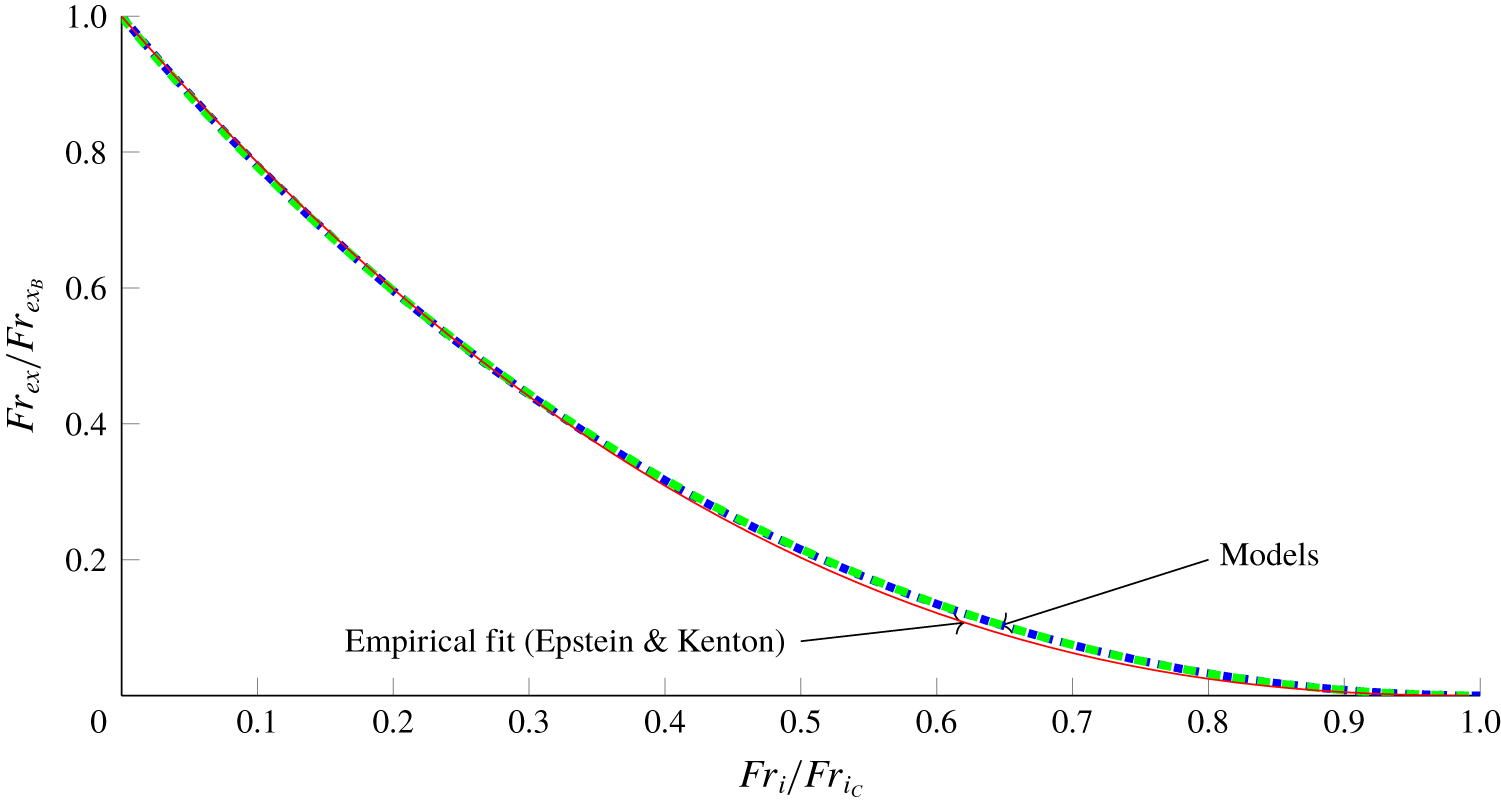
The theoretical predictions of § 6 (6.7) and § 7 ((7.4) and (7.10)) are plotted in figure 9 together with the empirical correlation (8.1) from Epstein & Kenton (Reference Epstein and Kenton1989). Figure 9 shows our theoretical predictions for unbalanced exchange collapsing such that they are almost graphically indistinguishable. They are also within  $\pm 0.01$ of the empirical correlation to the data of Epstein & Kenton (Reference Epstein and Kenton1989), equation (8.1). From the definition of the Froude number ratios it is necessary that (6.7), (7.11) and (8.1) all start at (0, 1), the balanced exchange limit, and finish at (1, 0), the unidirectional flow limit. The path of the line joining the two limits is dictated by the mode shape: for
 $Fr_{i}/Fr_{i_{C}}\ll 1$, small increases in imposed volume flux cause large decreases in the volume exchanged due to the steep gradients of the portion of the mode shape being advected across the opening (figures 5a and 8). Close to the critical imposed volume flux, the gradient of the perturbation near the plane of the opening is shallower, and so increases in the imposed volume flux result in smaller reductions of the exchange volume flux.
Volume flux for unbalanced exchange normalised against the balanced exchange volume flux as a function of the forcing (i.e. the imposed volume flow rate). Circular openings (6.7), dotted line; square openings (7.11), dashed line; and the empirical best fit from Epstein & Kenton (Reference Epstein and Kenton1989) (8.1), solid line. The lines for (6.7) and (7.11) (labelled ‘Models’) overlie each other so as to be graphically indistinguishable.

Our estimates of unbalanced exchange volume flux from §§ 6 and 7 were derived by extending a linear stability analysis of perturbations on an interface in the plane of a thin-walled opening beyond the linear region of behaviour. The empirical fit (8.1), by contrast, is valid for a range of opening aspect ratios from sharp-edged orifices to tubes.
Varrall et al. (Reference Varrall, Pretrel, Vaux and Vauquelin2017) extended their work on balanced exchange flows (Varrall et al. Reference Varrall, Pretrel, Vaux and Vauquelin2016) to unbalanced exchange flows, again using stereoscopic PIV and with  $Re\sim 10^{3}$. They imposed a flow rate below the critical flow rate such that there was unbalanced exchange, and measured the total volume flux
 $$\begin{eqnarray}Q_{tot}=Q_{i}+Q_{ex}.\end{eqnarray}$$
Their experiments used a relatively large density difference ( $(\unicode[STIX]{x1D70C}_{L}-\unicode[STIX]{x1D70C}_{U})/\unicode[STIX]{x1D70C}_{L}\approx 0.16$) so the Boussinesq approximation is no longer valid. However, a first-order correction to the Boussinesq theory developed in §§ 4–6 can be made by considering conservation of mass for the experimental compartment,
 $$\begin{eqnarray}\unicode[STIX]{x1D70C}_{U}Q_{tot}=\unicode[STIX]{x1D70C}_{L}Q_{i}+\unicode[STIX]{x1D70C}_{L}Q_{ex}.\end{eqnarray}$$
Rearranging and non-dimensionalising gives
 $$\begin{eqnarray}Fr_{tot}=\frac{\unicode[STIX]{x1D70C}_{L}}{\unicode[STIX]{x1D70C}_{U}}(Fr_{i}+Fr_{ex}).\end{eqnarray}$$
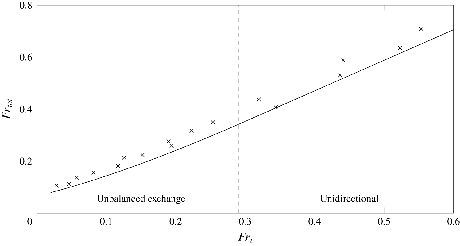
Figure 10 shows (8.4) plotted alongside the measurements of Varrall et al. (Reference Varrall, Pretrel, Vaux and Vauquelin2017), with  $Fr_{ex}$ taken from § 6 for
 $Fr_{i}<Fr_{i_{C}}=0.29$ and
 $Fr_{ex}=0$ for
 $Fr_{i}\geqslant Fr_{i_{C}}$. Equation (8.4) follows the trend of the data very well, however it marginally underestimates the experimental values of
 $Fr_{tot}$ (by 0.032, averaging across all experimental data); this is likely due to the crude nature of the correction employed to describe a non-Boussinesq system using a Boussinesq theory.
Plot of (8.4) (solid line) and experimental data of Varrall et al. (Reference Varrall, Pretrel, Vaux and Vauquelin2017) ( $\times$) with
 $0.2<L/D<0.3$. Equation (8.4) shows good agreement with the experimental data. The critical value of
 $Fr_{i_{C}}=0.29$ (to 2 s.f.), below which exchange would be expected, is indicated with a dashed line.

9 Applications
There are immediate applications of our unbalanced exchange flow model to the fluid mechanics of building ventilation, both for naturally and mechanically ventilated buildings. We consider such an application first (§ 9.1). Hunt & Coffey (Reference Hunt and Coffey2010) determine the geometrical conditions for which a buoyancy-driven flow gives rise to unbalanced exchange at an opening. For a warm room that ventilates via an opening in the top and in the base, they express this as a constraint on a Froude number associated with flow through the top opening. However, prior to the model developed herein there was no means for the prediction of the rates of air flow exchanged between the room and exterior under these conditions. We show how our model may be applied to the prediction of unbalanced exchange flow in buildings and discuss how our results have implications for the shape of opening chosen by a designer or architect.
Then (§ 9.2) we consider some of the implications of our findings to the source conditions of a nozzle intended to discharge buoyant fluid, for example, a nozzle used in laboratory studies of aqueous turbulent plumes (Baines & Turner Reference Baines and Turner1969; Cardoso & Woods Reference Cardoso and Woods1993; Kaye & Linden Reference Kaye and Linden2006) or a nozzle at the exit port of an ocean outfall. For these applications, it is desirable to prevent exchange flow from occurring.
9.1 Unbalanced exchange flow rates in naturally ventilated rooms
To retain the direction of the imposed flow adopted in §§ 1–8, i.e. vertically downward (figure 1a), the local density of air in the room  $\unicode[STIX]{x1D70C}_{U}=\unicode[STIX]{x1D70C}_{rm}$ must exceed the density of the external environment
 $\unicode[STIX]{x1D70C}_{L}=\unicode[STIX]{x1D70C}_{\infty }<\unicode[STIX]{x1D70C}_{rm}$ – i.e. the room is cool, and an exchange flow may develop at the base opening. For the inverted scenario, in which the imposed flow is upward, the room is warm and an exchange flow may develop at the top opening. In order to have a single and consistent identifier, that applies equally to warm- and cool-room scenarios, we instead label openings as primary (subscript
 $(\cdot )_{p}$) and secondary (subscript
 $(\cdot )_{s}$). Thus, in the cool-room scenario, the base opening has area
 $a=a_{p}$, and we introduce an opening at the top of the room of area
 $a_{s}$. The base opening is labelled ‘primary’ as only with
 $a_{p}>0$ is there an air flow under gravity. The top opening is ‘secondary’ as if the area
 $a_{s}>0$ there may (for
 $a_{p}>0$) or may not (for
 $a_{p}=0$) be flow, although as
 $a_{s}$ is varied it conditions the flow through the primary opening. With the ‘primary’ and ‘secondary’ terminology so introduced, if exchange flow is to occur, it will do so at the primary opening for both cool-room and warm-room scenarios.
The imposed flow in the natural ventilation application is that resulting from the differences in hydrostatic pressure between the interior and exterior environments (in a mechanical ventilation application, the imposed flow would be that set by a fan or pump). The Froude number, representing the dimensionless imposed flow rate, is  $Fr_{p,i}$ (
 $\equiv Fr_{i}$ in §§ 5–8). Within a displacement flow regime (Linden et al. Reference Linden, Lane-Serff and Smeed1990), flow is unidirectional through both primary and secondary openings, however Hunt & Coffey (Reference Hunt and Coffey2010) observed that for
 $Fr_{p,i}<0.33$ the flow at the primary opening was not unidirectional. Instead, a bidirectional flow was established in which fingers of buoyant fluid (occupying a fraction of this opening) would grow against the bulk outflow then pinch off, causing an exchange, i.e. there was unbalanced exchange flow.
Following Hunt & Coffey (Reference Hunt and Coffey2010), the buoyancy-driven imposed flow rate (upward or downward)  $Fr_{p,i}$ can be evaluated as
 $$\begin{eqnarray}Fr_{p,i}=\frac{Q_{p,i}}{a_{p}^{5/4}g{\displaystyle \frac{|\unicode[STIX]{x1D70C}_{rm}-\unicode[STIX]{x1D70C}_{\infty }|}{\unicode[STIX]{x1D70C}_{\infty }}}}=2^{1/2}\unicode[STIX]{x1D706}_{p}^{-1/2}\left(\frac{1}{c_{p}^{2}}+\frac{1}{c_{s}^{2}R^{2}}\right)^{-1/2},\end{eqnarray}$$
where
 $$\begin{eqnarray}R=\frac{a_{s}}{a_{p}},\quad \unicode[STIX]{x1D706}_{p}=\frac{\sqrt[]{a_{p}}}{h}.\end{eqnarray}$$
The constants  $c_{p}$ and
 $c_{s}$ are the loss coefficients associated with the primary and secondary openings respectively and
 $h$ is the depth of the layer of density
 $\unicode[STIX]{x1D70C}_{rm}$. The displacement flow limit is when the secondary opening has no discernible effect on the volume flow rate through the primary opening. Theoretically, this is achieved as
 $R\gg 1$ for
 $a_{p}>0$.
Having evaluated  $Fr_{p,i}$ using (9.1), the unbalanced exchange flow rate for this buoyancy-driven imposed flow may be evaluated on substituting for
 $Fr_{i}=Fr_{p,i}$ into the analysis presented in §§ 3–7. However, to facilitate the use of the theoretical developments by practitioners, including the non-specialist, polynomial best fit equations have been calculated to allow rapid, straightforward prediction of unbalanced exchange volume flux, while avoiding numerical integration. The relationships in figure 7 can be well approximated (maximum difference
 $=$ 0.0004) by the cubic
 $$\begin{eqnarray}Fr_{p,ex}=a_{1}Fr_{p,i}^{3}+a_{2}Fr_{p,i}^{2}+a_{3}Fr_{p,i}+a_{4},\end{eqnarray}$$
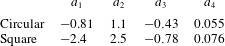
where the coefficients  $\{a_{1},a_{2},a_{3},a_{4}\}$ for each geometry are given in table 1. In balanced exchange,
 $Fr_{p,i}\equiv 0$, equation (9.3) reduces to
 $Fr_{p,ex}=a_{4}$. Table 1 gives
 $Fr_{p,ex}=0.055$ and
 $Fr_{p,ex}=0.076$ for a circular and square opening respectively, cf. (4.9) and (7.5). In a natural ventilation context one could achieve
 $Fr_{p,i}\equiv 0$ by closing the intake vent (
 $a_{s}\equiv 0$) and thus achieve a flow rate of 0.055 or
 $0.076\,a_{p}^{5/4}g^{\prime 1/2}~\text{m}^{3}~\text{s}^{-1}$ for a circular or square opening, respectively.
Coefficients of (9.3) for the calculation of the dimensionless unbalanced exchange volume flux (to 2 s.f.) through circular and square openings.

Beyond the predictive capability outlined above, a second implication of our work to room air flows is as follows. For a natural ventilation situation, where the aim is often to maximise the volume flux into the building, figure 7 shows that for a given area, a circular opening will result in a greater total flow rate than a square opening for  $Fr_{p,i}>0.088$. Therefore, if the majority of the operating range will be with
 $Fr_{p,i}>0.088$, a circular opening will result in greater flow rates, a result that may be useful for design. Conversely, for
 $Fr_{p,i}<0.088$ a square vent provides the higher flow rate. For some ventilation strategies, whether natural or mechanical, inflow at the exhaust opening (herein the primary opening) is undesirable, for example if it contravenes smoke ventilation regulations. With this in mind, beginning with
 $Fr_{p,i}\gg Fr_{p,i_{C}}$ and reducing the imposed flow rate, the analysis in § 7 suggests that unbalanced exchange will initiate at a circular opening before a square one, and, therefore, a square opening is more suitable in this context.
9.2 Source conditions that prevent bidirectional flow in nozzles
Another application of the theory developed is to the design and operation of plume nozzles, such as may be used in the laboratory modelling of ocean outfalls (e.g. Wilkinson Reference Wilkinson1988). Focus here is on nozzles that discharge fluid vertically. As discussed in § 1, a decrease in the dimensionless flow rate supplied to the nozzle,  $Fr_{i}$, i.e. the imposed flow rate, corresponds to the plume, that forms from the fluid discharged, becoming lazier (cf. Hunt & Kaye Reference Hunt and Kaye2005). Our analysis predicts, for a uniform velocity profile across the exit plane, that the operation of the nozzle is successful providing a critical outflow Froude number of
 $Fr_{i}\approx 0.3$ is met, or exceeded. If the flow rate imposed by the supply is lower, such that the outflow Froude number is below this value, an unbalanced exchange flow at the exit is to be anticipated. This is particularly undesirable in practice as the transport of sediment-laden salt water into the outfall can lead to a blockage (Wilkinson Reference Wilkinson1988).
10 Conclusions
We have developed and validated a mathematical model for predicting the flow rate associated with the vertical transport of fluid across an opening in a horizontal plane that connects two homogeneous bodies of miscible, incompressible, inviscid fluid of different density that are statically unstable and subject to an imposed flow rate through the opening. Triggered by buoyancy forces, finger-like instabilities that grow on the unstable interface in the plane of the opening pinch off and, thereby, exchange fluid (upward and downward) between the two fluid bodies. Our primary aim has been to predict the flow rates of this exchange for the general case in which the upward and downward flow rates are not equal in magnitude, so-called unbalanced exchange flow. The scales of the practical problems of interest are such that the exchanges are turbulent and the density differences are small compared with a characteristic reference density.
Reasoning that the transport of fluid across the opening is governed by the extent to which instabilities on the interface are able to grow against the opposing imposed flow, we model the volume of fluid pinched off as a function of the imposed flow rate and establish closed form solutions for the relative magnitudes of the upflow and downflow. We first focus on circular openings and then consider square openings. The relative time scales for the growth of the instabilities and the imposed flow rate give the scaling for unbalanced exchange flow and our governing parameter,  $Fr_{i}$.
When the imposed flow is zero, our model reduces to the limiting case of ‘balanced exchange flow’, in which the upflow and downflow are of equal magnitude. This was the single case considered by Epstein (Reference Epstein1988). As the imposed flow increases from zero, we predict that the volume flux exchanged across the opening decreases monotonically until a minimum, or critical, imposed flow rate is reached for which the instabilities are just swept out of the opening and the exchange flow ceases. At this minimum imposed flow velocity, our predictions agree with those of Linden et al. (Reference Linden, Lane-Serff and Smeed1990) for unidirectional flow through openings in a box.
In the context of building ventilation flows, our work is representative of the case in which a high-level vent in a flat roof links a warm interior environment to a cooler exterior. As such, our model for unbalanced exchange flows resolves the contradiction between the unidirectional (idealised displacement) flow theory of Linden et al. (Reference Linden, Lane-Serff and Smeed1990) and the balanced exchange flow theory of Epstein (Reference Epstein1988).
Our predictions show close agreement with the independent measurements of Epstein & Kenton (Reference Epstein and Kenton1989) and Varrall et al. (Reference Varrall, Pretrel, Vaux and Vauquelin2017) across the whole range of possible unbalanced flows. Moreover, our prediction of an imposed flow rate at the threshold between unbalanced exchange and unidirectional flow, a dimensionless critical imposed flow rate of 0.29 for circular vents, shows reasonable agreement with the value of 0.33 deduced from the measurements of Hunt & Coffey (Reference Hunt and Coffey2010). These findings indicate that the shape of the perturbation and our a priori treatment of the imposed velocity as uniform were not unreasonable.
That the limiting cases and threshold tally with existing theory and that good agreement with the data is achieved across the whole range of unbalanced exchange flows gives confidence in the practical use of the model as a predictive tool, for example, for use by architects and ventilation engineers in the control of air flows in modern buildings. To aid this practical application we provide polynomial fits to our theoretical results that allow the non-specialist to rapidly deploy the theoretical model developed herein.
Acknowledgements
The authors gratefully acknowledge the EPSRC for their financial support through the grant (EP/N010221/1) entitled Managing air for green cities (MAGIC). We would also like to thank three anonymous referees for their helpful suggestions.
Declaration of interests
The authors report no conflict of interest.
Appendix A. Why a separable variable solution is not possible
Sweeney et al. (Reference Sweeney, Kerswell and Mullin2013) investigated the Rayleigh–Taylor instability in an infinite vertical cylinder of radius  $R$, which requires solving
 $$\begin{eqnarray}\unicode[STIX]{x1D706}\boldsymbol{u}+\unicode[STIX]{x1D735}p=\frac{1}{Re}\unicode[STIX]{x1D6FB}^{2}\boldsymbol{u}\quad \text{and}\quad \unicode[STIX]{x1D735}\boldsymbol{\cdot }\boldsymbol{u}=0,\end{eqnarray}$$
subject to appropriate boundary conditions. Here  $\unicode[STIX]{x1D706}$ is the growth rate,
 $\boldsymbol{u}(u_{r},u_{\unicode[STIX]{x1D703}},u_{z})$ is the velocity,
 $p$ is the static pressure and
 $Re$ is the Reynolds number. They showed that for
 $z>0$ there are the separable solutions in cylindrical polar coordinates
 $(r,\unicode[STIX]{x1D703},z)$
 $$\begin{eqnarray}\displaystyle & u_{z}=(A_{1}\text{e}^{-kz}+A_{2}\text{e}^{-qz})\text{J}_{m}(kr)\text{e}^{\text{i}m\unicode[STIX]{x1D703}+\unicode[STIX]{x1D706}t}, & \displaystyle\end{eqnarray}$$
 $$\begin{eqnarray}\displaystyle & \displaystyle u_{r}=\frac{1}{2}\left(A_{1}\text{e}^{-kz}+A_{2}\frac{q}{k}\text{e}^{-qz}\right)(\text{J}_{m+1}(kr)-\text{J}_{m-1}(kr))\text{e}^{\text{i}m\unicode[STIX]{x1D703}+\unicode[STIX]{x1D706}t}, & \displaystyle\end{eqnarray}$$
 $$\begin{eqnarray}\displaystyle & \displaystyle \text{i}u_{\unicode[STIX]{x1D703}}=\frac{1}{2}\left(A_{1}\text{e}^{-kz}+A_{2}\frac{q}{k}\text{e}^{-qz}\right)(\text{J}_{m+1}(kr)+\text{J}_{m-1}(kr))\text{e}^{\text{i}m\unicode[STIX]{x1D703}+\unicode[STIX]{x1D706}t}, & \displaystyle\end{eqnarray}$$
 $$\begin{eqnarray}\displaystyle & \displaystyle p=\frac{\unicode[STIX]{x1D706}}{k}(A_{1}\text{e}^{-kz})\text{J}_{m}(kr)\text{e}^{\text{i}m\unicode[STIX]{x1D703}+\unicode[STIX]{x1D706}t}, & \displaystyle\end{eqnarray}$$
where  $q=\sqrt{k^{2}+\unicode[STIX]{x1D706}Re}$, with corresponding solutions of similar form in
 $z<0$. In the above,
 $\text{i}=\sqrt{-1}$ is the imaginary unit,
 $\text{J}_{m}$ is the Bessel function of the first kind of order
 $m$, and
 $k$ is the radial wavenumber, of which there will be a different value for each
 $m$. The constants
 $A_{1}$ and
 $A_{2}$ are arbitrary.
An important feature of these solutions is that the boundary condition of no fluid penetration through the cylinder walls can be set using only one coordinate, that is we require  $u_{r}=0$ on
 $r=R\;\forall z$. There is no dependence on
 $\unicode[STIX]{x1D703}$ or
 $z$ and we are not interested in the solution for
 $r>R$, i.e. outside the cylinder.
By contrast, if we consider a circular opening of radius  $R$ in an infinite horizontal plane at
 $z=0$ (figure 1a), we can no longer express the no-penetration boundary condition, which is now
 $u_{z}=0$ on
 $z=0$ for
 $r>R$, using only one coordinate. This means we cannot have a straightforward variable separable solution that meets the boundary condition. The only way to ensure that
 $u_{z}=0$ on
 $z=0$ for
 $r>R$ is with
 $A_{1}=A_{2}=0$, however this means
 $u_{z}$ and also
 $u_{r},u_{\unicode[STIX]{x1D703}}$ and
 $p$ are identically zero throughout the whole domain. Whilst this is a solution, it is trivial and offers no insight.
More generally, assume we could find a different separable solution for the vertical velocity  $u_{z}=f(r)\unicode[STIX]{x1D6E9}(\unicode[STIX]{x1D703})h(z)$ such that
 $f(r)$ was zero for
 $r>R$ but not for
 $r<R$ – i.e. precisely the form needed in the plane of the opening. This would ensure no penetration through the plane but also that
 $u_{z}=0$ throughout the fluid for
 $r>R$ (i.e. at all
 $z$) when there is no physical reason for this to be the case. Alternatively, we could assume we could find
 $h(z)$ such that
 $h(0)=0$, meeting the no-penetration boundary condition but also preventing exchange across the opening. Therefore, a separable solution that satisfies the boundary conditions is not possible.
Appendix B. Calculation of the radial wavenumber  $k$

For balanced exchange flow the volumes enclosed by the perturbation (4.3) above and below the plane of the opening must be equal (figure 5a). Therefore,
 $$\begin{eqnarray}2\unicode[STIX]{x03C0}\hat{\unicode[STIX]{x1D702}}\int _{0}^{r_{1}}r(\text{J}_{0}(kr)-\text{J}_{0}(kD/2))\,\text{d}r=-2\unicode[STIX]{x03C0}\hat{\unicode[STIX]{x1D702}}\int _{r_{1}}^{D/2}r(\text{J}_{0}(kr)-\text{J}_{0}(kD/2))\,\text{d}r\end{eqnarray}$$
 $$\begin{eqnarray}\displaystyle \Rightarrow \frac{r_{1}\text{J}_{1}(kr_{1})}{k}-\frac{r_{1}^{2}\text{J}_{0}(kD/2)}{2} & = & \displaystyle \frac{r_{1}\text{J}_{1}(kr_{1})}{k}-\frac{r_{1}^{2}\text{J}_{0}(kD/2)}{2}-\frac{D\text{J}_{1}(kD/2)}{2k}+\frac{D^{2}\text{J}_{0}(kD/2)}{8}\nonumber\\ \displaystyle & & \displaystyle\end{eqnarray}$$
 $$\begin{eqnarray}\displaystyle & \Rightarrow & \displaystyle \text{J}_{1}(kD/2)=\frac{kD\text{J}_{0}(kD/2)}{4}.\end{eqnarray}$$
This has roots  $kD=10.27$, 16.83, 23.24, (to 4 s.f.) etc. However, only with
 $kD=10.27$ does the perturbation have the observed form (Varrall et al. Reference Varrall, Pretrel, Vaux and Vauquelin2016), with a single central region of rising fluid and a single outer annulus of descending fluid. The condition
 $\unicode[STIX]{x1D702}(r_{1})=0$ implies
 $\text{J}_{0}(kr_{1})=\text{J}_{0}(kD/2)$, for which the only solution for
 $kr_{1}<kD/2$ is
 $kr_{1}=2.7$ (to 2 s.f.), so that
 $2r_{1}/D=0.52$ (to 2 s.f.).