
1. Introduction
Point-vortex decomposition of the vorticity field in two-dimensional flows of ideal incompressible fluid was introduced firstly by Helmholtz in 1858, and later this problem was formulated in Hamiltonian form by Kirchhoff in 1877. Although the notion of a point vortex is an idealization, it is directly related to real vortex flows. As Kizner (Reference Kizner2014) writes ‘A point vortex can be thought of as a limit, in which, say, a Gaussian vortex shrinks into a point while retaining the net vorticity (or potential vorticity). The point-vortex concept becomes particularly suitable when it comes to exploring the interactions between remote vortices. By employing this concept we replace a continuous dynamical system, which describes a vortical flow, by a discrete one’. In other words, this approach is supposed to work well when the separation between the vorticity patches is large enough compared with the sizes of the patches. This is exactly the case in vortex scattering, which is the focus of this paper. An example of a successful oceanographic application of a configuration with a small number of point vortices is the explanation for the complex behaviour of the anticyclone eddy observed in the Bay of Biscay in 1990, given in terms of the movement of a strongly perturbed vortical tripole with a significant separation between the core and satellite eddies (Kizner et al. Reference Kizner, Shteinbuch-Fridman, Makarov and Rabinovich2017). In this work, the results obtained with point-vortex tripoles barely differed from those obtained with grid simulations.
Within the point-vortex approach, numerous studies, including generalizations to spherical geometry, domains with boundaries and fluid with layered stratification, were carried out ever since (see e.g. reviews in Aref et al. Reference Aref, Kadtke, Zawadzki, Campbell and Eckhardt1988; Aref, Rott & Thomann Reference Aref, Rott and Thomann1992; Newton Reference Newton2001, Reference Newton2014; Borisov & Mamaev Reference Borisov and Mamaev2005; Sokolovskiy & Verron Reference Sokolovskiy and Verron2014). A more sophisticated extension of the point-vortex concept to singular vortices embedded in a regular flow in the presence of the β-effect was discussed in a few publications dealing with both single-layer (barotropic) and multi-layer models (Reznik Reference Reznik1992; Reznik & Kizner Reference Reznik and Kizner2007a,Reference Reznik and Kiznerb, Reference Reznik and Kizner2010; Kravtsov & Reznik Reference Kravtsov and Reznik2019). But even with conventional single-layer vortices that are considered in this present paper, in general, the problem is non-integrable for more than three vortices. The non-trivial case of three vortices was first investigated by Gröbli (Reference Gröbli1877). Synge (Reference Synge1949) used trilinear coordinates for the description of the dynamics of three vortices, having analysed, in particular, singular and stationary points of the phase space. Works of Novikov (Reference Novikov1975) and Aref (Reference Aref1979) gave rise to intensive studies of various aspects of the point-vortex dynamics. Linear stability analysis for relative equilibria of three vortices was performed by Tavantzis & Ting (Reference Tavantzis and Ting1988) and Aref (Reference Aref2009). The dynamics of four vortices with zero total intensity and impulse (when the problem is integrable) was studied by Eckhardt (Reference Eckhardt1988) and Aref & Stremler (Reference Aref and Stremler1999). Many papers deal with finding equilibria (not only symmetrical) of more than three vortices and analysis of their stability (e.g. Aref & Vainchtein Reference Aref and Vainchtein1998; Aref et al. Reference Aref, Newton, Stremler, Tokieda and Vainchtein2003; Aref Reference Aref2007; Chen, Kolokolnikov & Zhirov Reference Chen, Kolokolnikov and Zhirov2013; Kurakin, Ostrovskaya & Sokolovskiy Reference Kurakin, Ostrovskaya and Sokolovskiy2016). In particular, Roberts (Reference Roberts2013) and Hampton, Roberts & Santoprete (Reference Hampton, Roberts and Santoprete2014) presented stationary configurations of four vortices comprising of two pairs with equal strengths, including collinear configurations, rhombuses, isosceles trapezoids, kite-like structures and a set of asymmetric stationary states. Considering two-layer quasi-geostrophic flows, Kizner (Reference Kizner2006) introduced the concept of a hetonic quartet, a collinear ensemble of two point-vortex hetons, and studied their nonlinear stability. Nonlinear stability of point-vortex multipoles in the barotropic and two-layer fluid was investigated by Kizner (Reference Kizner2011, Reference Kizner2014), who based his analysis on two invariants of motion which depend on intervortical distances only.
The phenomenon of self-similar collapse or expansion (when the initial geometrical form is preserved and only the size of the configuration decreases or increases) was discovered by Gröbli (Reference Gröbli1877) for three vortices and then it was studied in detail (see e.g. Synge Reference Synge1949; Novikov & Sedov Reference Novikov and Sedov1979; Kimura Reference Kimura1990; Borisov & Lebedev Reference Borisov and Lebedev1998; Newton Reference Newton2001), including cases with a large number of vortices (Demina & Kudryashov Reference Demina and Kudryashov2014; Kudela Reference Kudela2014). It is known (Synge Reference Synge1949) that intervortical distances are bounded if the strengths of all the vortices have the same sign. Otherwise, vortex scattering can occur, characterized by the fact that some intervortical separations increase to infinity. Two evident examples (and probably mechanisms) of scattering are: emission of a dipole and a self-similar complete extension, which take place even in the simplest case of three vortices. For more vortices, clustering into relatively separated groups is possible.
The main objective of this paper is the investigation of possible mechanisms of group scattering of vortices (as a certain analogue of molecular diffusion) on the unbounded plane. In these processes, only the relative motion of the vortices matters, therefore in § 2 we introduce an invariant function of relative motion which depends on the intervortex separations only and is a combination of the first integrals of the system. A general necessary condition of scattering as an asymptotic process is also formulated. Considering only the geometrical form of an ensemble of N vortices, one can express the invariant function through 2N−4 independent variables in a polar coordinate system. This function can be used to construct stationary configurations, i.e. relative equilibria, and to investigate their nonlinear stability. In § 3 we apply this approach to three vortices, where the invariant function depends on two variables only, namely, the ratio of the lengths of any of two sides of the vortex triangle and the angle between them. The periodic absolute motion of three vortices, which consists of two alternating stages of expansion and convergence of the vortex ensemble, is considered in § 4. Scattering of three vortices (including emission of a dipole) is examined in detail in § 5; in particular, an asymptotically self-similar scattering is described, and sufficient conditions for such a regime are formulated. Application of the invariant function to analyse the evolution of centrally symmetric configurations of five (or four) vortices is considered in § 6, where the relevance of this restriction to real vortex flows is briefly discussed. Possible mechanisms of group scattering are demonstrated in § 7 with the example of five vortices. In § 8 an example of group scattering of 1009 vortices with strengths randomly distributed in the interval (−1, 1) is discussed. The absolute motion of N point vortices was calculated using the fourth-order Runge–Kutta method with adaptive time step control (Press et al. Reference Press, Teukolsky, Vetterling and Flannery1996).
2. Relative motion of point vortices
2.1. The invariant function
For unbounded ideal fluid, planar motion of an ensemble of N point vortices with strengths  $\gamma _n$ and coordinates
 $(x_n,y_n)$ occurs with conservation of the Hamiltonian H (i.e. interaction energy), combined invariant M and the total vortex momentum L
 \begin{gather}H = -\displaystyle{1 \over {4{{\rm \pi} }}}\sum\limits_{n = 1}^{N-1} {\sum\limits_{k = n + 1}^N {\gamma _n\gamma _k\log (r_{nk}^2 )} ,} \end{gather}
 \begin{gather}M = \Gamma J-I_x^2 -I_y^2 = \sum\limits_{n = 1}^{N-1} {\sum\limits_{k = n + 1}^N {\gamma _n\gamma _kr_{nk}^2 } } ,\end{gather}
 \begin{gather}L = 2{{\rm \pi} }\sum\limits_{n = 1}^N {\gamma _n(x_n\,\hbox{d}y_n/\hbox{d}t-y_n\,\hbox{d}\kern0.06em x_n/\hbox{d}t)} = \sum\limits_{n = 1}^{N-1} {\sum\limits_{k = n + 1}^N {\gamma _n\gamma _k} } ,\end{gather}
where  $r_{nk}$ are intervortex separations. Here,
 $\Gamma = \sum\nolimits_{n = 1}^N {\gamma _n} $ is the total circulation,
 $J = \sum\nolimits_{n = 1}^N {\gamma _n(x_n^2 + y_n^2 )} $ is the angular momentum,
 $I_x = \sum\nolimits_{n = 1}^N {\gamma _nx_n} $,
 $I_y = \sum\nolimits_{n = 1}^N {\gamma _ny_n} $ are the components of the linear momentum; all are conserved quantities. Note that
 $M = \Gamma J$ when the origin of the coordinates system lies in the centre of vorticity
 $(I_x/\Gamma ,I_y/\Gamma )$. The system of 2N equations
 $\gamma _n\,\hbox{d}\kern0.06em x_n/\hbox{d}t = \partial H/\partial y_n$,
 $\gamma _n\,\hbox{d}y_n/\hbox{d}t = -\partial H/\partial x_n$ describes the absolute motion of N vortices.
Considering relative motion as the evolution of the geometrical form of an ensemble of vortices, we can use polar coordinates with origin at the position of any vortex (the first for definiteness) and a reference polar axis that contains the segment  $r_{12}$ (again for definiteness). Choosing then the magnitude of
 $r_{12}$ as a variable space scale, one can introduce 2(N−2) independent variables: polar angles
 $\varphi _n$ and scaled radii
 $\rho _n = r_{1n}/r_{12},\;n \ge 3$, which uniquely define geometrical form (but not its size, position and orientation in space) of the vortex configuration at any time.
For  $r_{nk} = r_{12}\tilde{r}_{nk}$,
 $n = 1, \ldots ,N,\;k \gt n$, where
 $\tilde{r}_{nk}$ are the normalized intervortex separations, the expressions (2.1) and (2.2) become
 $H = \tilde{H}-L\log (r_{12}^2 )/(4{{\rm \pi} })$ and
 $M = r_{12}^2 \tilde{M}$, where
 $\tilde{H} = H(\tilde{r}_{nk})$,
 $\tilde{M} = M(\tilde{r}_{nk})$. Thus, the invariants of motion (2.1)–(2.3) can be combining into one invariant function of relative motion which depends on the above-defined normalized phase variables only
 \begin{align} F& = -4{{\rm \pi} }H-L\log |M| = -4{{\rm \pi} }\tilde{H}-L\log |\tilde{M}|\nonumber\\ & = \gamma _1\sum\limits_{n = 3}^N {\gamma _n\log (\rho _n^2 )} + \sum\limits_{n = 2}^{N-1} {\gamma _n} \sum\limits_{k = n + 1}^N {\gamma _k\log [\rho _n^2 + \rho _k^2 -2\rho _n\rho _k\cos (\varphi _n-\varphi _k)]} -L\log |R|,\end{align}
where a scaled function
 \begin{equation}R = \tilde{M} = M/r_{12}^2 = \sum\limits_{n = 2}^N {\gamma _n(\Gamma -\gamma _n)\rho _n^2 -2} \sum\limits_{n = 2}^{N-1} {\gamma _n\rho _n} \sum\limits_{k = n + 1}^N {\gamma _k\rho _k\cos (\varphi _n-\varphi _k)} ,\end{equation}
is introduced and  $\varphi _2 = 0,\;\rho _2 = 1$. The cosine rule is used here to express the intervortex separations
 $r_{nk}$ at
 $n \gt 1,\;k \gt n$.
The invariant function F, in fact, represents the Hamiltonian H restricted to a level surface of the invariant M. An isoline of this function represents the evolution of geometrical shapes of a vortex ensemble, but not of its sizes (because of the normalization on r 12). More rigorously, from this point on, we are discussing the behaviour of a new dynamical system with the phase space  $(\varphi _3,\rho _3, \ldots ,\varphi _N,\rho _N)$, in which the absolute motion and orientation of a vortex ensemble are ignored and geometrically similar configurations of vortices are indistinguishable. Only in this sense shall we talk below of phase trajectories, stationary points (or equilibria) and their stability. For example, now not only conventional relative equilibria, but also a self-similarly expanding or collapsing vortex ensemble becomes represented in this phase space by a stationary point, whose stability/instability may be interpreted as stability/instability of the non-stationary self-similar motion. A solution of a set of equations
 $\partial F/\partial \varphi _n = 0,\;\partial F/\partial \rho _n = 0$ gives stationary points in the phase space, i.e. equilibrium configurations. The type of these points (maximum/minimum or saddle) defines the nonlinear stability of the corresponding stationary state. To do this, it is enough to calculate the eigenvalues of the Hessian, a square matrix of second-order partial derivatives of the invariant function.
2.2. Necessary condition for group scattering
In addition to stationary points in the phase space  $(\varphi _3,\rho _3, \ldots ,\varphi _N,\rho _N)$, there are also singular points induced by the logarithmic terms in the invariant function. The set of these points determines the topology of the phase space and (qualitatively) the evolution of a given vortex configuration depending on its initial location in this space. If the phase trajectory touches some singular point (or curve), the initially N-vortex system asymptotically splits into certain independent groups of vortices. When not all of the circulations of the individual vortices have the same sign, some intervortical distances may increase to infinity. For example, an N-vortex system during the well-known self-similar motion can either break up to N infinitely distant vortices (within infinite time), or collapse in one point within finite time (with the velocity growing to infinity). In the case of three vortices (see e.g. Newton Reference Newton2001) the necessary and sufficient condition for self-similar complete scattering/collapse is simultaneous vanishing of the invariants L and M (or R). Nevertheless, at any N, the invariant function remains finite, as directly follows from its definition (2.4).
A necessary condition for complete group scattering can be derived as follows. Let N vortices cluster during the evolution into K groups ( $1 \lt K \le N$) with the circulations
 $\Gamma _k$ (the sum of strengths of all vortices belonging to kth group). Clustering and the hypothetical scattering of the groups mean that the intervortex separations remain finite within each group only. Therefore, the invariants of motion H and M will remain finite only if the summarized contribution of the terms in (2.1) and (2.2) tending to infinity is zero. After regrouping the terms, the sought-for necessary condition for group scattering takes the form
 \begin{equation}L_G = \sum\limits_{k = 1}^{K-1} {\sum\limits_{m = k + 1}^K {\Gamma _k\Gamma _m} } = 0.\end{equation}
Here,  $L_G$ is the group analogue of the total vortex momentum L. Condition (2.6) is also valid in the case of emission of inseparable groups with zero group circulation.
3. Relative motion of three vortices revisited
3.1. Invariant function and singular points
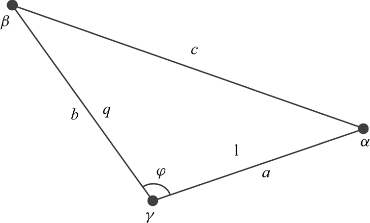
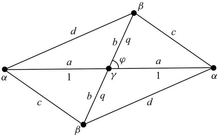
Consider now three vortices with strengths  $\gamma _1 = \gamma ,\;\gamma _2 = \alpha ,\;\gamma _3 = \beta $ (see figure 1). Setting
 $\varphi _3 = \varphi ,\;\rho _3 = b/a = q$ in formulae (2.4) and (2.5), we will obtain the following expression for the invariant function
 \begin{equation}F(\varphi ,q) = -L\log |R(\varphi ,q)| + \beta \gamma \log q^2 + \alpha \beta \log P(\varphi ,q),\end{equation}
where
 \begin{gather}P(\varphi ,q)\equiv c^2/a^2 = q^2-2q\cos \varphi + 1,\end{gather}
 \begin{gather}R(\varphi ,q) = \beta (\alpha + \gamma )q^2-2\alpha \beta q\cos \varphi + \alpha (\beta + \gamma ),\end{gather}
 \begin{gather}L = \alpha \gamma + \beta \gamma + \alpha \beta .\end{gather}
Parameters of three vortices in the plane; a, b and c are dimensional, 1 and q, normalized sizes.

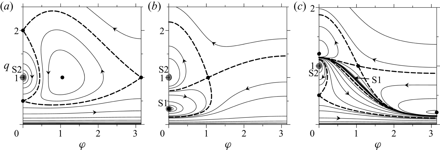
The invariant function is 2 ${\rm \pi}$-periodic and symmetric relative to the vertical axis
 $\varphi = {{\rm \pi} }$. Except for the cases where emission or complete scattering can occur, all phase trajectories are either 2
 ${\rm \pi}$-periodic or closed (see examples in figure 2). Periodicity of phase trajectories, however, does not mean strict periodicity of the absolute motion on the
 $(x,y)$ plane.
Phase diagrams of the relative motion of three vortices at (a)  $\alpha = \beta = \gamma = 1$
 $(\Gamma = 3,\;L = 3)$; (b)
 $\alpha = 0.5,\;\beta = -1.5,\;\gamma = 1$
 $(\Gamma = 0,\;L = -1.75)$; (c)
 $\alpha = 1,\;\beta = -0.75,\;\gamma = 1$
 $(\Gamma = 1.25,\;L = -0.5)$. Black solid circles mark the stationary points representing collinear equilibria at
 $\varphi = 0,{{\rm \pi} }$ and the equilateral triangle at
 $\varphi = {\rm \pi}/3,\;q = 1$; dashed bold lines, the separatrices passing through the saddle points. Grey circles mark the singular points S2; bold solid line in (c), singular curve S1. Arrows indicate the direction of motion in the phase trajectories.

For any set of strengths, the phase diagram necessarily includes a singular point with coordinates (0, 1) for which  $P(\varphi ,q) = 0$. In this point two of the three vortices ‘merge’ into one ‘vortex’ and the initial problem reduces to N = 2. So, hereinafter we will refer to this type of singularity as S2. The same reduction occurs also at
 $q = 0$ and
 $q = \infty $. In the phase diagrams presented in figure 2 points S2 appear as centres.
Singular points of another type, S1 (when the initial problem may reduce to N = 1, see below), fill the curve described by the equation  $R(\varphi ,q) = 0$. The condition for the existence of the singular curve S1 is easily derived using (3.3):
 \begin{equation}s = \gamma \Gamma /(\alpha \beta ) \lt 0.\end{equation}
If the strengths of all vortices have the same sign (figure 2a), curve S1 does not exist. If  $\Gamma = 0$ (figure 2b), S1 consists of one point which is the stationary point
 $(0,-\alpha /\beta )$ at
 $\alpha /\beta \lt 0$ or
 $({{\rm \pi} },\alpha /\beta )$ at
 $\alpha /\beta \gt 0$. In the phase diagram, this point is represented by the centre. Generally (see figure 2c), the curve S1 consists of a set of points, in each of which the local infinite extremum of the invariant function is reached, while the Hamiltonian of the system is finite.
At  $L = 0$ the curve S1 (where
 $R = 0$) presents a set of initial vortex configurations, for which the motion becomes self-similar, i.e. either total scattering or collapse occurs. At
 $L\ne 0$ curve S1 in the phase diagram represents a special line in which the absolute motion is periodic. We will discuss some features of such a motion in § 4.
3.2. Nonlinear stability of equilibria
Stationary states, or equilibria, of three vortices and their linear stability were investigated earlier by Tavantzis & Ting (Reference Tavantzis and Ting1988) and Aref (Reference Aref2009). Here we search for equilibria and analyse their nonlinear stability using the invariant function F. Its partial derivatives are
 \begin{gather}F_\varphi = Aq\sin \varphi ,\quad F_q = A(q-\cos \varphi ) + Cq,\end{gather}
 \begin{gather}F_{\varphi \varphi } = Aq\cos \varphi -Bq^2\sin ^2\varphi ,\end{gather}
 \begin{gather}F_{qq} = A + C-B(q-\cos \varphi )^2-Dq^2 + 2Eq(q-\cos \varphi ),\end{gather}
 \begin{gather}F_{\varphi q} = F_{q\varphi } = [A-Bq(q-\cos \varphi ) + Eq^2]\sin \varphi ,\end{gather}
where
 \begin{equation}\left. \begin{gathered}A = 2\alpha \beta \left( {\displaystyle{1 \over P}-\displaystyle{L \over R}} \right),\quad B = 4\alpha \beta \left( {\displaystyle{1 \over {P^2}}-\displaystyle{{\alpha \beta L} \over {R^2}}} \right),\quad C = 2\beta \gamma \left( {\displaystyle{1 \over {q^2}}-\displaystyle{L \over R}} \right),\\ D = 4\beta \gamma \left( {\displaystyle{1 \over {q^4}}-\displaystyle{{\beta \gamma L} \over {R^2}}} \right),\quad E = \displaystyle{{4\alpha \beta^2\gamma L} \over {R^2}}.\end{gathered}\right\}\end{equation}
As seen from (3.6) and (3.8), the condition of vanishing  $F_\varphi $ and
 $F_q$ determining the stationary points is
 \begin{equation}\left. \begin{gathered} q(R-LP)\sin \varphi = 0,\\ \alpha q(q-\cos \varphi )(R-LP) + \gamma P(R-Lq^2) = 0. \end{gathered}\right\}\end{equation}
When a stationary point is found, its type and hence the nonlinear stability of the corresponding equilibrium is defined by the sign of the Hessian determinant
 \begin{equation}G = F_{\varphi \varphi }F_{qq}-F_{\varphi q}F_{q\varphi }.\end{equation}
At positive (negative) G, a stationary point in the phase plane is a centre (saddle), and the corresponding equilibrium is stable (unstable).
Two cases follow from the first equation in (3.9): either  $R-LP = 0$ or
 $\sin \varphi = 0$. In the first case, (3.9) take a simple form
 \begin{equation}\left. \begin{gathered} R-LP = 0,\\ R-Lq^2 = 0. \end{gathered} \right\}\end{equation}
At  $L\ne 0$ the system has a single solution
 $\varphi = {{\rm \pi} }/3,\;q = 1$; that is an equilateral triangle which is the relative equilibrium existing at any set of strengths (see figure 2). For this solution P = 1 and R = L, coefficients A and C in (3.8) are equal to zero, and the Hessian determinant (3.10) is easily calculated,
 $G = 0.75(BD-E^2) = 12(\alpha \beta \gamma )^2/L$. Thus, equilateral triangles are unstable at L < 0 and are nonlinearly stable at L > 0 (in particular, equilateral triangles with zero total circulation are all unstable). The same result was obtained using trilinear coordinates by Synge (Reference Synge1949). Also, the nonlinear stability of the equilateral triangle with equal strengths of vortices was shown by Kizner (Reference Kizner2014). At
 $L = 0$ the equilateral triangle is stable according to Aref (Reference Aref2009). Some details of this case will be considered in § 5.
In the second case, when  $\sin \varphi = 0$, two sets of the stationary points (at
 $\varphi = 0$ and
 $\varphi = {{\rm \pi} }$) satisfy (3.9), both corresponding to collinear vortex equilibria. Let
 \begin{equation}\sigma = \cos \varphi = \begin{cases} + 1, & {\varphi = 0},\\ {-1,}& {\varphi = {{\rm \pi} }}.\end{cases}\end{equation}
Then, with the exception of singular solutions, the cubic equation
 \begin{equation}(\alpha + \gamma )q^3-\sigma (2\alpha + \gamma )q^2-(2\beta + \gamma )q + \sigma (\beta + \gamma ) = 0,\end{equation}
can be derived for determination of the collinear stationary states. Positive real roots of (3.13) define equilibria at given strengths. A similar equation (obtained in a different way) already appeared in Tavantzis & Ting (Reference Tavantzis and Ting1988) for the case  $\sigma = 1$ and in Aref (Reference Aref2009) for the case
 $\sigma = -1$ (see also Borisov & Lebedev Reference Borisov and Lebedev1998). Note that for collinear configurations the second term in the Hessian determinant (3.10) vanishes due to (3.7c).
In some special cases, relationship (3.13) can be simplified. For example, at  $\alpha = \beta = \gamma $ one obtains three stationary saddle points (0, 0.5), (0, 2) and
 $({{\rm \pi} },1)$ in the phase diagram (see figure 2a). Direct calculation shows that the Hessian determinant is negative in these points. In fact, these three stationary points represent the same symmetric collinear configuration. Topologically, however, all three points are important since the separatrices divide the phase space into areas with different behaviours of phase trajectories.
When two vortices have equal (e.g. unit) strengths, there are two symmetric collinear equilibria in the points (0, 0.5) and  $({{\rm \pi} },1)$, for which the central vortex can be of arbitrary strength
 $\lambda $. The Hessian determinant (3.10) for both stationary points is proportional to
 $-(4\lambda + 5)[\lambda /(\lambda + 2)]^2$. From here the necessary and sufficient condition
 $\lambda \lt -1.25$ for nonlinear stability is obtained. The same result was obtained earlier by Kizner (Reference Kizner2014), who used another nonlinear approach, and by Aref (Reference Aref2009) and Kurakin et al. (Reference Kurakin, Ostrovskaya and Sokolovskiy2016) within the linear stability analysis. Note that in the interval
 $-1.25 \lt \lambda \lt -0.5$ the equilateral triangle and one of the collinear configurations can both be unstable (see figure 2c).
Equation (3.13) can be written in an alternative form
 \begin{equation}R^{(\sigma )}(q)\left( {q-\sigma \displaystyle{\gamma \over {\Gamma -\beta }}} \right)-L\displaystyle{{\Gamma + \beta } \over {\Gamma -\beta }}\left( {q-\sigma \displaystyle{{\Gamma -\alpha } \over {\Gamma + \beta }}} \right) = 0,\end{equation}
where  $R^{(\sigma )}(q) = \beta (\Gamma -\beta )q^2-2\alpha \beta \sigma q + \alpha (\Gamma -\alpha )$ is derived from (3.3) using (3.12). At
 $L = 0$ and
 $R^{(\sigma )}\ne 0$ from (3.14) follows the solution
 $q = -\sigma \beta /\alpha $ representing the known fixed (i.e. motionless) collinear equilibrium (see e.g. Newton Reference Newton2001). Direct substitution of this solution in (3.7) gives
 $F_{\varphi \varphi } = -2\gamma ^2 \lt 0$,
 $F_{qq} = 2(\alpha \gamma /\beta )^2 \gt 0$, therefore, all fixed collinear equilibria are unstable. This statement was earlier proved in the linear approximation by Aref (Reference Aref2009).
At zero total circulation,  $\Gamma = 0$, the single solution following from (3.14) is the singular solution S1 (see figure 2b). For this solution,
 $R = 0$, therefore, it is necessary to use asymptotic analysis for estimation of the sign of the Hessian determinant. Since the coefficient at the term
 $L/R^2$ in the expression for
 $F_{qq}$ vanishes, the leading terms in
 $F_{\varphi \varphi }$ and
 $F_{qq}$ which define the sign of G are
 $2\alpha ^2L/R$ and
 $2\beta ^2L/R$, respectively. The product of these two infinite quantities is always positive, therefore, any collinear equilibrium with zero total circulation is nonlinearly stable. Earlier, Aref (Reference Aref2009) proved the linear stability of such configurations, and Kizner (Reference Kizner2011, Reference Kizner2014) proved their nonlinear stability at
 $\alpha = \beta $.
4. Periodic absolute motion of three vortices
Periodicity of absolute motion with  $\Gamma \ne 0$ means the synchronous return of all vortices to the initial position on the
 $(x,y)$ plane within some time
 $T_a$. The absolute (physical) vortex trajectories are closed in this case, however, can be intricate. The simplest example of such a motion is solid-state rotation of a stable relative equilibrium when vortices move along circular orbits. More complicated periodic absolute motion is executed in the case when the combined invariant M (or, R) of the ensemble of vortices is zero. In addition, due to definition (2.2), at
 $\Gamma \ne 0$ the linear and angular momenta calculated with respect to the vorticity centre are also zero. Some examples of periodic absolute motion (but without a direct declaration about it) in a case where two vortices have equal strengths, were considered by Leoncini et al. (Reference Leoncini, Kuznetsov and Zaslavsky2001).
The manifold of points  $(\varphi ,q)$, in which
 $R = 0$, is the singular curve S1. Thus, a necessary condition for periodic absolute motion is condition (3.5), i.e. the value of
 $s = \gamma \Gamma /(\alpha \beta )$ should be negative. At
 $s \le -1$ the curve S1 is a
 $2{{\rm \pi} }$-periodic function (see examples in figures 2c and 3a). At
 $-1 \lt s \lt 0$ the closed in this case curve S1 is defined on the interval
 $-\varphi _{\lim } \lt \varphi \lt \varphi _{\lim }$ if
 $\gamma /\alpha \gt -1$, and on the interval
 ${{\rm \pi} }-\varphi _{\lim } \lt \varphi \lt {{\rm \pi} } + \varphi _{\lim }$ at
 $\gamma /\alpha \lt -1$, where
 $\varphi _{\lim } = \arccos \sqrt {s + 1} $. The period of the absolute motion
 $T_\alpha $ is always multiple to the period of the relative motion
 $T_r$, the time during which the vortex configuration takes again the initial geometrical form.
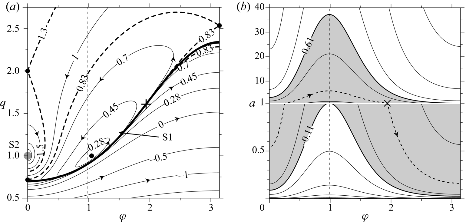
Isolines of (a) the invariant function  $F(\varphi ,q)$, and (b) the Hamiltonian
 $E_R(\varphi ,a)$ at
 $\alpha = -0.45,\;\beta = \gamma = 1\;(L = 0.1)$. The bold cross labels the initial configuration
 $(\varphi _0 = 0.6175{{\rm \pi} },\;q_0\approx 1.608,\;a_0 = 1)$ used in the simulation presented in figure 4. Arrows and numbers indicate the direction of motion and the values of the function on the isolines. The vertical dashed lines (
 $\varphi \approx 0.985$) mark the point where parameter a takes its maxima on the isolines of
 $E_R$. In (a) black solid circles mark stationary points; dashed bold lines are the separatrices passing through saddle points; grey solid circle marks the singular point S2; bold solid line, singular curve S1. In (b) dashed bold line is the isoline of
 $E_R$ passing through the initial state; grey domain marks the range of
 $E_R$ values.

Although the invariant function at  $L\ne 0$ keeps an infinite value on S1, this curve (bold line in figure 3a) is not a phase trajectory because the finite value taken by the Hamiltonian H is not constant, being dependent on the position of the initial point on S1. Topologically, curve S1 is a barrier that divides the phase plane into domains with opposite directions of traveling along trajectories. The Hamiltonian on S1 can be regarded as proportional to a function of two variables only,
 $\varphi $ and one of the intervortical distances, say, a (see figure 1)
 \begin{equation}E_R(\varphi ,a) = -4{{\rm \pi} }H(\varphi ,a) = L\log a^2 + \beta \gamma \log q_R^2 (\varphi ) + \alpha \beta \log P_R(\varphi ),\end{equation}
where  $q_R(\varphi )$ is the positive solution of the equation
 $R = 0$,
 $P_R = -\gamma [\beta q_R^2 (\varphi ) + \alpha ]/\alpha \beta \ne 0$. The behaviour of
 $E_R$ is shown in figure 3(b), where parameter a is scaled with its initial value
 $a_0$. The straight line
 $a = 1$ in figure 3(b) represents the set of vortex configurations lying on S1 in figure 3(a). In other words, for any initial point with
 $\varphi = \varphi _0$, the intervortical distance a is defined by the isoline crossing the straight line
 $a = 1$ at
 $\varphi = \varphi _0$ in figure 3(b).
From the equation of this isoline,  $E_R(\varphi ,a) = E_R(\varphi _0,1)$, an explicit expression for the distance a is obtained
 \begin{equation}a(\varphi;\varphi _0) = \{ [q_R(\varphi _0)/q_R(\varphi )]^\gamma [P_R(\varphi _0)/P_R(\varphi )]^{\alpha /2}\} ^{\beta /L}.\end{equation}
Since  $\partial a/\partial \varphi = -a\beta (2\gamma P_R\partial q_R/\partial \varphi + \alpha q_R\partial P_R/\partial \varphi )/(2Lq_RP_R)$, the extremum condition for the function
 $a(\varphi;\varphi _0)$ takes the form
 $(\partial q_R/\partial \varphi )(P_R-q_R^2 ) = 0$. At
 $\partial q_R/\partial \varphi = 0$ we obtain
 $\varphi _{ex} = 0$ or
 $\varphi _{ex} = {{\rm \pi} }$ and, respectively,
 $q_R = \alpha \beta (\sigma \pm \sqrt {-s} )/(L-\alpha \gamma )$, where
 $\sigma $ is defined by formula (3.11) and the sign is chosen so that
 $q_R \gt 0$. At
 $P_R = q_R^2 $ we find
 $\varphi _{ex} = arccos(0.5/q_R)$, where
 $q_R^2 = \alpha \gamma /(\alpha \gamma -L)$. That is, the extremum is reached either on collinear configurations or on isosceles triangles. Note that the ratio of the maximal value of a to its minimal value,
 $A_s = a(\varphi _{max};\varphi _0)/a(\varphi _{min};\varphi _0) = a(\varphi _{max};\varphi _{min})$, depends on the vortex strengths only. The values
 $\varphi = \varphi _{ex}$ divide the straight line
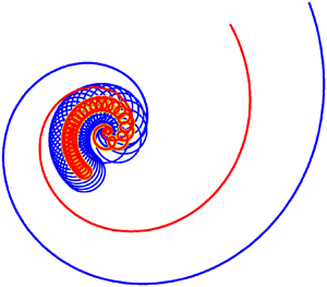
 $a = 1$ and, respectively, the curve S1 (see figure 3) into areas where a monotonically increases or decreases. That is, periodic absolute motion (see figure 4) consists of the alternate stages of expansion and convergence of vortices. Absolute trajectories of vortices in both stages have spiral form. The space and time scales within the stages of the motion can significantly differ depending on the value of
 $A_s$. For the case presented in figures 3 and 4 where
 $L = 0.1$, we have
 $A_s\approx 37.2$; when
 $L = 0.01$ the magnitude of this parameter exceeds 1015. Some phase trajectories with non-zero M can be partly attracted by the curve S1; thus, the absolute motion corresponding to these trajectories can include stages of sizeable expansion and compact convergence of vortices. Expansion prevails in time.
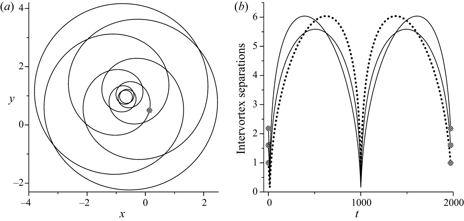
Periodic absolute motion of three vortices at  $R = 0$ in simulation starting from the point
 $\varphi _0 = 0.6175{{\rm \pi} },\;q_0\approx 1.608$ at
 $\alpha = -0.45,\;\beta = \gamma = 1\;(L = 0.1)$. (a) Trajectory of the geometrical centre of three vortices. (b) Time dependences of intervortex separations (dotted line for a) during one period
 $T_a\approx 1971.13$. Black solid circles show initial and final positions on the plots.

A result of numerical simulation of the absolute motion is shown in figure 4(a) only for the physical trajectory of the geometrical centre of three vortices; individual vortex trajectories have similar forms. The behaviour of intervortex separations is shown in figure 4(b).
5. Scattering of three vortices
5.1. Complete scattering
Consider now a case where functions R and L both vanish. In this case, (3.9) turn into identities, thus all points of the singular curve S1 become stationary points where the geometrical form of three vortices remains unchanged with time. On the other hand, the solutions at  $R = 0$ considered in § 4 cease being periodic in the limit
 $L\to 0$ and only expansion or convergence of vortices are possible for each point on S1 except for points corresponding to the relative equilibria. Such kind of motion is known as self-similar motion (Gröbli Reference Gröbli1877; Synge Reference Synge1949; Newton Reference Newton2001; Aref Reference Aref2010).
At  $L = 0$, condition (3.5) for the existence of the singular curve S1 is automatically satisfied, and equation for determining the configurations that expand or collapse self-similarly takes the form
 \begin{equation}R = q^2-2(\mu + 1)q\cos \varphi + \mu = 0,\quad \mu = \beta /\alpha .\end{equation}
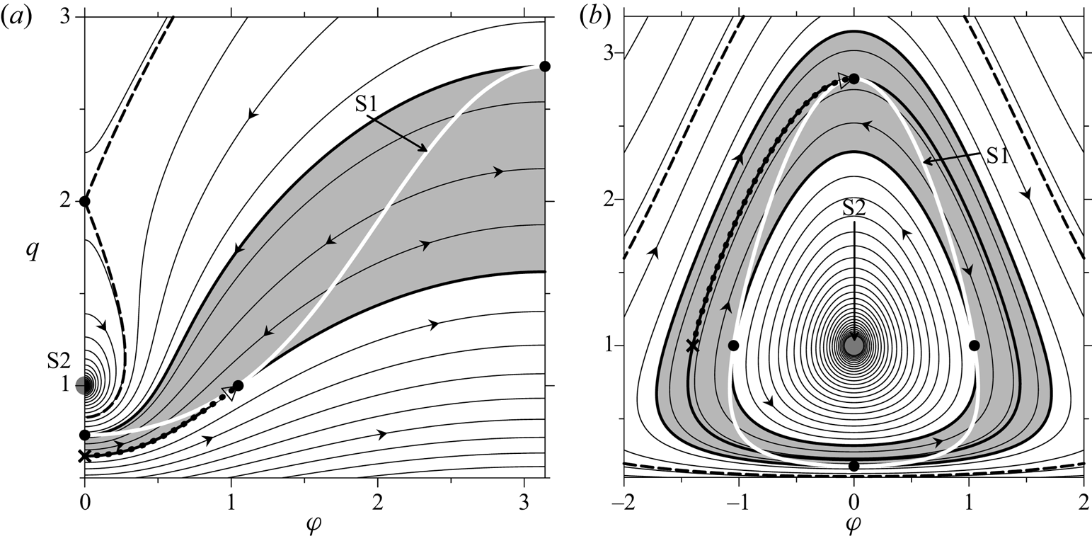
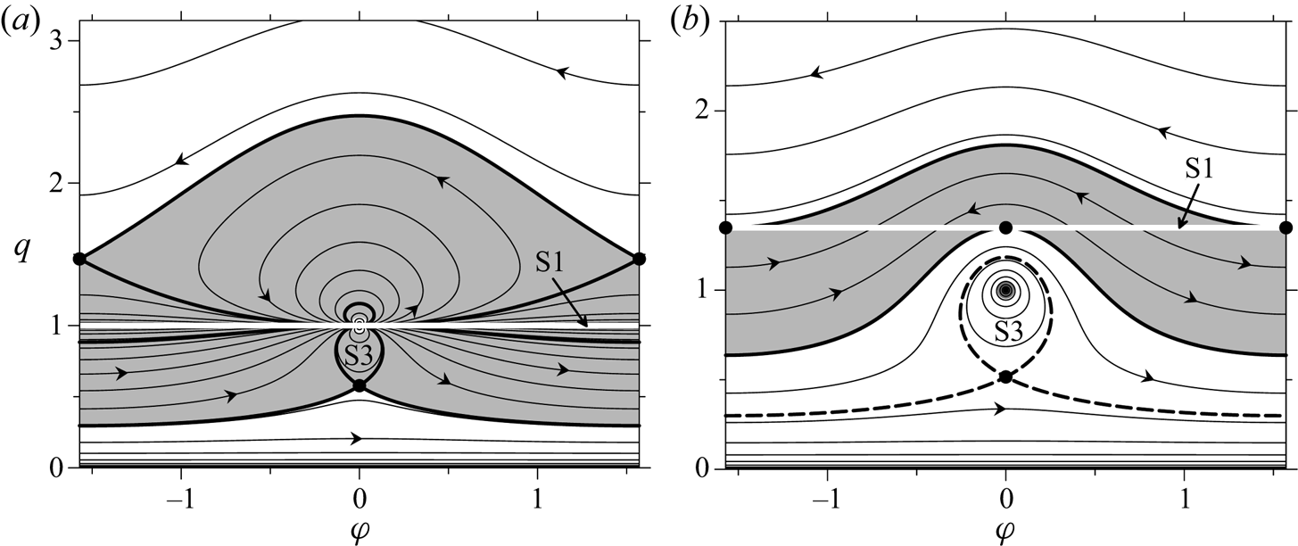
At different points of the line S1, function F now takes different finite values, and each isoline that crosses S1 is divided in the crossing point into parts with opposite directions of passing through (compare figures 3a and 5). The crossing points in which the two parts of an isoline converge (diverge) represent a vortex configuration that expands (collapses) self-similarly. The points on S1 which correspond to relative equilibria (dark solid circles in figure 5) divide S1 into segments within which only collapse or expansion occurs. The relative equilibria on S1 are the equilateral triangle in points  $( \pm {{\rm \pi} }/3,1)$, and two collinear states at
 $\varphi = 0$ and/or
 $\varphi = {{\rm \pi} }$ with positive
 $q = \sigma (\mu + 1) \pm \sqrt {\mu ^2 + \mu + 1} $.
Phase diagrams of relative motion of three vortices at  $L = 0$ and (a)
 $\alpha = -0.5,\;\beta = \gamma = 1$; (b)
 $\alpha = -3,\;\beta = -1.5,\;\gamma = 1$. Bold white line, singular curve S1; grey solid circle, singular point S2. Dark solid circles, stationary points. The scattering domain is shaded by grey. Bold dark lines pass through stable relative equilibria; bold dashed lines are saddle point separatrices. Dotted lines show phase trajectories obtained in numerical simulations presented in figure 6; cross and hollow triangle mark the starting and the ending points.

At  $L\to 0$ and
 $R\to 0$ one can derive from (3.7), (3.8) that
 $F_{\varphi \varphi }\to k_{\varphi \varphi }^2 L/R^2$,
 $F_{qq}\to k_{qq}^2 L/R^2$,
 $F_{\varphi q}\to k_{\varphi \varphi }k_{qq}L/R^2$, where
 $k_{\varphi \varphi } = 2\alpha \beta q\sin \varphi $ and
 $k_{qq} = -2\alpha (\gamma q + \beta \cos \varphi )$. Hence, within these limits, the Hessian determinant (3.10) vanishes. But, since in points on S1 that corresponds to self-similar expanding (or collapsing) states the phase trajectories converge (or diverge), these states are stable (or unstable). Relative equilibria are stable. The same results were earlier obtained using linear approximation by Tavantzis & Ting (Reference Tavantzis and Ting1988), Kimura (Reference Kimura1990) and Aref (Reference Aref2010). At
 $L = 0$, in the phase diagrams (figure 5) there are also a singular point S2 (presented by centre) and a saddle point
 $(0,-\beta /\alpha )$ or
 $({{\rm \pi} },\beta /\alpha )$; the latter corresponds to an unstable fixed collinear equilibrium (Aref Reference Aref2009; see also § 3.2).
Curve S1 and all phase trajectories that cross it lie completely in the domain (shaded by grey in figure 5) which is bounded by the isolines of F passing through the points representing the equilateral triangle and one of the collinear states. Starting the motion from any interior point (with  $R\ne 0$) of this domain we will asymptotically approach some point Z on S1 (note that the phase diagram is symmetric about the straight line
 $\varphi = {{\rm \pi} }$). In the absolute motion, this appears as asymptotic scattering: all intervortex separations increase to infinity, but the changing geometrical form of the configuration tends to the triangle at the point Z. It is clear also that
 $R\to 0$ at
 $t\to \infty $. Thus, the necessary condition for asymptotic scattering is
 $L = 0$, and the sufficient condition is belonging of the initial state to the above-mentioned domain which can be called the scattering domain. The collapse is more delicate; it can occur for self-similar motion only when both R and L vanish.
It is known (e.g. Newton Reference Newton2001; Aref Reference Aref2010) that the trajectories of the vortices in a self-similar motion are similar logarithmic spirals, and the intervortex separations increase or decrease in proportion to  $(1 + \tau t)^\kappa $ with
 $\kappa = 1/2$, where parameter
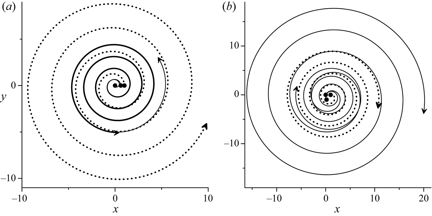
 $\tau $ depends on the initial vortex configuration. Our numerical simulations show that, in general, this is correct with good accuracy for the asymptotically self-similar scattering too.
Two examples of asymptotic scattering are presented in figure 6(a,b) for the combinations of strengths as in figure 5(a,b) respectively. In the first case, the initially collinear (but not stationary) state asymptotically transforms into an equilateral triangle (dotted curve in figure 5a). The initial point  $(0,q_0)$ in the phase plane (the cross in figure 5a) is located at the lower boundary of the scattering domain, where
 $q_0\approx 0.618$ is the solution of the equation
 $F(0,q_0) = F({{\rm \pi} }/3,1) = 0$. In the second example, the initial point
 $(\varphi _0,1)$, where
 $\varphi _0\approx -1.402$ is the solution of the equation
 $F(\varphi _0,1) = F(0,q_s)$, is placed at the phase trajectory passing through the point
 $(0,q_s)$ which corresponds to the collinear equilibrium with
 $q_s = 0.5(3 + \sqrt 7 )$. In this case, where the initial state is an isosceles triangle, the configuration asymptotically transforms into a collinear state (dotted curve in figure 5b).
Asymptotic scattering at  $L = 0$ (but
 $R\ne 0$) for combinations of strengths and initial vortex configurations as in figures 5(a) and 5(b) respectively. Trajectories of the absolute motion of three vortices (dotted line, the vortex with the strength
 $\alpha $) are shown. Black solid circles and arrows show the initial and the final (at
 $t = 3000$) positions.

Some features of motion when both L and R are small but not equal to zero are discussed in Leoncini et al. (Reference Leoncini, Kuznetsov and Zaslavsky2000) for the case of two equal strengths.
5.2. Emission of a translating dipole
The necessary condition for emission of a dipole translating to infinity is vanishing of its total circulation. Under this condition L becomes negative, hence the stationary point  $({{\rm \pi} }/3,1)$, which corresponds to equilateral triangle on the phase plane, is a saddle point. The stationary points corresponding to collinear equilibria are defined at
 $\alpha + \beta = 0$ by the equation
 $(q-\sigma )[(\eta + 1)q^2-\sigma \eta q + (\eta -1)] = 0$, where
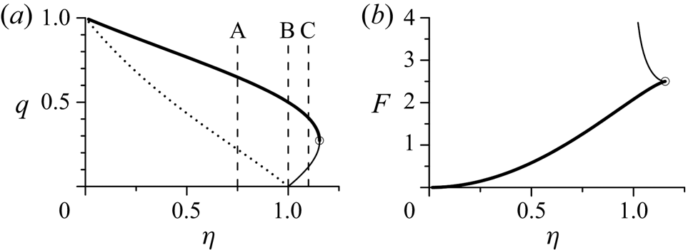
 $\eta = \alpha /\gamma $. In addition to the singular solution S2, this equation describes two branches of collinear equilibria (at
 $\sigma = \pm 1$) which exist at
 $|\eta |\le 2/\sqrt 3 $ (see figure 7a). At
 $\sigma = -1$ (when
 $\varphi = {{\rm \pi} }$), the Hessian determinant G is always positive, hence, the corresponding equilibria are stable. At
 $\sigma = 1$ (when
 $\varphi = 0$) G takes negative values in the interval
 $2-\sqrt 3 \lt q \lt 2 + \sqrt 3 $. In the points where
 $\eta = \pm 2/\sqrt 3 $,
 $F_{qq} = 0$, and the plot of the invariant function F calculated over stationary points changes its behaviour here (figure 7b). Since
 $q(-\eta ) = 1/q(\eta )$ and
 $F(-\eta ) = F(\eta )$ the plots in figure 7 are presented for positive
 $\eta $ only.
(a) Collinear relative equilibria at  $\alpha + \beta = 0$ on the
 $(\eta = \alpha /\gamma ,q)$ plane; solid (dotted) lines represent solutions at
 $\varphi = 0$ (
 $\varphi = {{\rm \pi} }$). Vertical dashed lines A, B and C pass through
 $\eta = 0.75$, 1 and 1.1, respectively. (b) Invariant function F calculated over collinear equilibria with
 $\varphi = 0$. Solutions on bold solid lines are unstable; blank circle is the point in which stability changes to instability.

In the case of emission of a dipole the singular curve S1 always exists, and at  $\alpha + \beta = 0$ its form is described by the equation
 $R = (\eta + 1)q^2-2\eta q\cos \varphi + (\eta -1) = 0$, which also has the singular solution of S2 type in the point (0, 1). In the special case,
 $\eta = 1$ or
 $\eta = -1$, when there exist two pairs of vortices with zero group circulation, the equation
 $R = 0$ reduces to equalities
 $q = \cos \varphi $ or
 $q\cos \varphi = 1$, which describe a set of rectangular triangles. In these cases curve S1 either goes to infinity, asymptotically approaching the straight line
 $\varphi = \pm {{\rm \pi} }/2$, or it tends to approach the point
 $( \pm {{\rm \pi} }/2,0)$. The points at
 $q = \infty $ or
 $q = 0$ are the singular points of S2 type by its definition in § 3.1 Thus, in all cases, S1 asymptotically approaches the singular point S2, in which the dynamics of three vortices actually turns into the dynamics of two vortices. In terms of absolute motion, this directly implies the emission of a dipole. In the phase plane not only singular curve S1 is attracted by the point S2; there also exists a manifold of trajectories that are attracted by S2 and are entirely located inside some domain, which will be termed the emission domain. Outside this domain, the phase trajectories are closed or periodic.
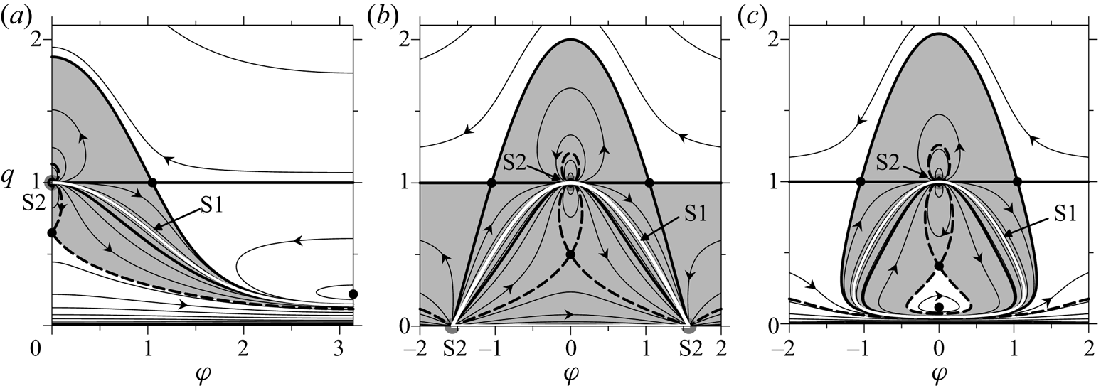
Examples of phase diagrams are presented in figure 8. At  $|\eta |\lt 1$ (figure 8a) the boundaries of the emission domain are
 $2{{\rm \pi} }$-periodic. At
 $1 \lt |\eta |\lt 2/\sqrt 3 $, the finite emission domain is multiply connected (figure 8c) because of the existence of two branches in the family of collinear equilibria at
 $\varphi = 0$ (see figure 7a). At
 $|\eta |\gt 2/\sqrt 3 $ there is only one equilibrium, the unstable equilateral triangle, and the emission domain is bounded by a closed branch of the separatrix described by the equation
 $F(\varphi ,q) = \alpha ^2\ln \alpha ^2$. The aforementioned special case
 $\eta = 1$ (i.e.
 $\alpha = -\beta = \gamma $) is presented in figure 8b. Note that if the starting point is set on S1, the absolute motion of the individual vortices is executed along parallel straight lines while the vortex triangle remains rectangular. An example of such an evolution (but only its initial stage without mentioning of emission) was considered by Gröbli (Reference Gröbli1877); see also Aref et al. (Reference Aref, Rott and Thomann1992).
Phase diagrams of relative motion of three vortices at  $\alpha + \beta = 0$,
 $\gamma = 1$. (a)
 $\alpha = 0.75$ (line A in figure 7a); (b)
 $\alpha = 1$ (line B); and (c)
 $\alpha = 1.1$ (line C). Shaded is the emission domain. Bold dark (dashed) lines pass through the saddle points corresponding to the equilateral triangle (collinear equilibrium). Other notations as in figures 2 and 5.

In a dipole, which translates to infinity, the intervortical distance tends to  $d = a_0q_0^{1/\eta } \sqrt {q_0^2 -2q_0\cos \varphi _0 + 1} $. This can be derived by equating the Hamiltonians of the limiting dipole and the initial configuration of three vortices.
6. Vortex configurations with central symmetry
6.1. Relative motion and stability of five vortices
Consider now a centrally symmetric configuration in which four vortices are located in the vertices of a parallelogram, and the fifth is located in the geometrical centre. Vortices at the opposite ends of diagonals are assumed to have the same strengths (see figure 9). In general, the invariant function F depends on six phase variables (see § 2.1). However, often, in numerical simulations and laboratory experiments, unstable vortex ensembles, initially possessing central symmetry, practically retain it in the course of their evolution, even when no special restrictions are imposed (e.g. Trieling, van Heijst & Kizner Reference Trieling, van Heijst and Kizner2010). The assumption of keeping the central symmetry makes it possible to reduce the dimension of the phase space to two. Kizner (Reference Kizner2011, Reference Kizner2014) proposed such a consideration for the case where four or three peripheral vortices have equal strength. In our case, one can derive the expression for the invariant function F which depends on two variables only. Using the designations  $q = b/a,\;p = c/a,\;h = d/a$ (by analogy with the case N = 3) we obtain
 \begin{equation}F(\varphi ,q) = -L\log |R(q)| + \beta (\beta + 2\gamma )\log q^2 + 2\alpha \beta \log P(\varphi ,q),\end{equation}
where now
 \begin{gather}P(\varphi ,q)\equiv p^2h^2 = q^4-2q^2\cos 2\varphi + 1,\end{gather}
 \begin{gather}R(q) = \alpha + \beta q^2,\end{gather}
 \begin{gather}L = 2(\alpha \gamma + \beta \gamma + \alpha \beta ) + (\alpha + \beta )^2.\end{gather}
In expression (6.1) the term  $C_F = -L\log |\Gamma | + [2(\alpha ^2 + \beta ^2)-L]\log 2$ with
 $\Gamma = \gamma + 2(\alpha + \beta )$, is omitted as a constant. Due to the symmetry, M is presented by the angular momentum only, and the function R is independent of
 $\varphi $. The invariant function F is
 ${{\rm \pi} }$-periodic and symmetric with respect to
 $\varphi = {{\rm \pi} }/2$.
Scheme of the relative arrangement of five vortices with central symmetry; a, b, c and d are dimensional, 1 and q, normalized sizes.

On the phase plane  $(\varphi ,q)$ there are singular points with coordinates
 $(0,1)$,
 $(\varphi ,0)$ or
 $(\varphi ,\infty )$. These points (of S3 type) represent the limiting symmetric tripole resulting either from pairwise ‘merger’ (collapse) of the peripheral vortices (of the original configuration), which creates the two satellites of the tripole, or from the ‘merger’ of two peripheral vortices and the central vortex (of the original configuration), which creates the central vortex of the tripole. The singular curve S1 (where
 $R = 0$) has the same sense, as in the case of three vortices, representing either limiting transition to five independent vortices, or collapse to one vortex, both at
 $L = 0$. According to (6.3), S1 is a straight line
 $q = \sqrt {-\alpha /\beta } $ and exists when
 $\alpha $ and
 $\beta $ have opposite signs. At
 $L\ne 0$ line S1, as for three vortices, represents a locus of initial vortex configurations which are periodic in absolute motion (when the central symmetry is kept).
Since  $F_\varphi = 8\alpha \beta q^2\sin 2\varphi /P$, equilibria with central symmetry can be only collinear configurations, at
 $\varphi = 0$, or rhombuses with a central vortex, at
 $\varphi = {{\rm \pi} }/2$. Designating
 \begin{equation}\sigma = \cos 2\varphi = \begin{cases} { + 1,} & {\varphi = 0}, \\ {-1,} & {\varphi = {{\rm \pi} }/2},\end{cases}\end{equation}
from the equation  $F_q = 0$ we derive the relation for both families of stationary points
 \begin{equation}R[(\alpha + 2\gamma )q^2-\sigma (2\Gamma -3\alpha )]-L(q^2-\sigma ) = 0.\end{equation}
Since  $F_{\varphi q} = F_{q\varphi } = 0$ at the stationary points, a function
 \begin{equation}g = -4R^2-\sigma L(q^2-\sigma )^2, \end{equation}
which completely defines the sign of the Hessian determinant, can be derived. From consideration of (6.7) it is seen that rhombuses at  $L \le 0$ and collinear states at
 $L \ge 0$ are unstable. In particular, at
 $\alpha = \beta $ for a square (when
 $\varphi = {{\rm \pi} }/2,\;q = 1$) direct substitution to (6.7) gives the instability condition
 $\alpha (\alpha + 2\gamma ) \lt 0$ obtained earlier (in a different way) by Kizner (Reference Kizner2011, Reference Kizner2014). In case of zero total circulation (when L is always negative) all rhombuses are unstable, but collinear equilibria can be stable relative to perturbations which obey the central symmetry; from here, however, stability to unrestricted perturbations does not follow.
6.2. Symmetrical scattering of five vortices
Consider first the situation when two dipoles formed by peripheral vortices move away from the motionless central vortex in opposite directions. A necessary condition for such a development is  $\alpha + \beta = 0$. Because this condition entails
 $L = -2\alpha ^2$ and
 $R = \alpha (1-q^2)$, all equilibria (rhombuses at
 $q^2 = (3\eta \pm 2\sqrt {2\eta ^2 + 1} )/(2 + \eta )$ and collinear states at
 $q^2 = (2-\eta )/(2 + \eta )$ where
 $\eta = \alpha /\gamma $) are unstable due to (6.7), i.e. all stationary points are saddles. The singular point S3 at
 $\beta = -\alpha $ formally represents an unstable collinear equilibrium and lies on the singular line S1. Topologically (see figure 10a) this point attracts all phase trajectories entirely located in the emission domain (shaded in the plot), bounded by separatrices passing through stationary saddle points. Thus, the dipole emission is only possible for the vortex configurations represented by the points lying inside this domain.


For the complete scattering (where  $L = 0$), from (6.7) it follows that all equilibria described by relation (6.6) are unstable, except for the case
 $R = 0$. When both L and R are zero, the singular line S1 is a set of isolated points for which self-similar motion with keeping the position of the central vortex takes place. As for the case of three vortices, on the phase plane (figure 10b) there exists the scattering domain where, for any interior point, asymptotic scattering (without keeping form) occurs.
6.3. Relative motion of four vortices
This case follows from the previous one under the assumption that  $\gamma = 0$ in formulae (6.1)–(6.7). Two families of equilibria (collinear states at
 $\sigma = 1$ and rhombuses at
 $\sigma = -1$) are defined by the relation
 $q^4-[(4 + \sigma ) + (1 + 4\sigma )\mu ]q^2 + \sigma \mu = 0$ where
 $\mu = \beta /\alpha $. From (6.7) it follows that the equilibria of both types are unstable at
 $q^2 \lt q_1^2 = 2-\sqrt 3 $ and
 $q^2 \gt q_2^2 = 2 + \sqrt 3 $, and are stable (with respect to symmetrical perturbations) in the interval
 $(q_1^2 ,q_2^2 )$. Similar results were reported by Roberts (Reference Roberts2013) who constructed and investigated for stability stationary solutions for rhombuses, thought in a different way. Collinear equilibria of four vortices were considered by Hampton et al. (Reference Hampton, Roberts and Santoprete2014). As follows from our general approach with the use of four phase variables in this case (not presented here), rhombuses in the interval
 $(q_1^2 ,q_2^2 )$ remains stable also with respect to general perturbations, but collinear equilibria do not.
The change from stability to instability (or vice versa) occurs at  $\mu = \mu _{1,2} = -2\mp \sqrt 3 $ (when
 $L = 0$) in the stationary points
 $(0,q_{1,2})$ and
 $({{\rm \pi} }/2,q_{1,2})$. In these points
 $\mu q^2 + 1 = 0$ (i.e.
 $R = 0$), thus they lie on the line S1. All other points from S1 represent the configurations that undergo self-similar scattering/collapse of four vortices. The same criterion of self-similarity (
 $q^2 = -1/\mu = 2 \pm \sqrt 3 $) was derived earlier by Novikov & Sedov (Reference Novikov and Sedov1979). The domain on the phase plane, in which all four-vortex configurations undergo asymptotic scattering can be found by analogy with the case of N = 5.
For four centrally symmetric vortices, the necessary condition of dipole emission is zero total circulation. Since the linear momentum is also equal to zero, the system becomes integrable and can be reduced to the relative motion of three vortices (Eckhardt Reference Eckhardt1988; Rott Reference Rott1990; Aref & Stremler Reference Aref and Stremler1999). The initial symmetry is kept in this case. At  $\Gamma = 0$ there are only unstable rhombus equilibria with
 $q^2 = 3 \pm 2\sqrt 2 $; separatrices passing through corresponding saddle points bound the emission domain on the phase plane where any initial vortex configuration eventually breaks up into a pair of dipoles moving in opposite directions.
The invariant function depending only on two variables can be constructed also under the condition that, for all times, the configuration can be obtained by mirror symmetry reflection of a pair of vortices relative to a straight line, the physical interpretation of this case being the motion of two vortices near an impenetrable solid wall. Clearly, the four vortices form an isosceles trapezoid in this case. Relative equilibria of two pairs of vortices with equal strengths considered by Roberts (Reference Roberts2013) and Hampton et al. (Reference Hampton, Roberts and Santoprete2014) also have this shape.
7. Group scattering of five vortices
We consider now examples of group scattering for the case of five vortices with three different strengths  $(\alpha ,\beta ,\gamma )$ which initially form a centrally symmetric configuration. In this case, the number of various scenarios of splitting into groups is 26, but not all of them satisfy the necessary condition (2.6). In the case considered below with the strengths
 $(-1,2,1)$, there are only three different variants of group scattering: (A) emission of a dipole
 $(\alpha ,\gamma )$ and possible scattering of the remaining three vortices
 $(\beta ,\beta ,\alpha )$ for which
 $L = 0$; (B) emission of three vortices
 $(\alpha ,\beta ,\alpha )$ with zero total circulation; and (C) complete scattering of three groups in a combination
 $\beta ,(\alpha ,\beta ,\gamma ),\alpha $ or
 $\beta ,\beta ,(\alpha ,\alpha ,\gamma )$. In case (C), both combinations give the same distribution of group strengths
 $(2,2,-1)$ for which
 $L = 0$, while, for a group of three vortices, emission of a dipole
 $(\alpha ,\gamma )$ can occur, which may end up as case (A). The specific type of evolution (including the scenario at which scattering is not realized) depends on the initial geometrical configuration of vortices.
All the three above-described scenarios of group scattering are shown in figures 11(a), 11(b) and 11(c), respectively. As initial states, collinear configurations with  $\varphi _0 = 0$ at different values of
 $q_0$ were chosen for these simulations. In all simulations, the initial symmetry is lost and grouping is observed. Since in every scenario a vortex triad forms, it is possible to use the three-vortex phase diagram as a tool for diagnostics of the motion. To do so, we represent the group by its rotation centre. Projections of calculated phase trajectories onto the phase plane of three vortices with group strengths
 $(\bar{\alpha },\bar{\beta },\bar{\gamma })$ are shown in figure 12. For variants (A) and (C) these projections after some time arrive at the scattering domain (see figure 12a). For the case of emission of three vortices (variant B), the phase trajectory for this triad approaches asymptotically one of the periodical isolines (figure 12b). In the variant (C) for vortex triad participating in scattering as a group, the phase trajectory stabilizes near a closed isoline around the singular point S2, outside the emission domain (see figure 12c). Therefore this triad robustly moves along a spiral trajectory (figure 11c).
Trajectories of absolute motion for different scenarios of group scattering of five vortices at  $\alpha = -1,\;\beta = 2,\;\gamma = 1$, which initially form a collinear configuration with
 $\varphi = \varphi _0 = 0$ and
 $q = q_0$. (a) Variant (A): emission of a dipoile
 $(\alpha ,\gamma )$ and subsequent complete scattering of three vortices
 $(\beta ,\beta ,\alpha )$ at
 $q_0 = 0.685$;
 $t = 150$. (b) Variant (B): emission of a vortex triad
 $(\alpha ,\beta ,\alpha )$ at
 $q_0 = 0.69$;
 $t = 50$. (c) Variant (C): scattering of three groups of vortices
 $\beta ,(\alpha ,\beta ,\gamma ),\alpha $ at
 $q_0 = 0.4$;
 $t = 3000$. Solid grey circles and arrows indicate the initial and final positions of vortices, except for the dipole in plot (a) that covers the distance of about 140 space units within
 $t = 150$.

Projections of phase trajectories (dotted lines marked by capitals) calculated from numerical simulations with five vortices onto the phase plane of three vortices with strengths  $(\bar{\alpha },\bar{\beta },\bar{\gamma })$ at (a)
 ${\rm \; }\bar{\alpha } = 2,\;\bar{\beta } = 2,\;\bar{\gamma } = -1$; (b)
 $\bar{\alpha } = 1,\;\bar{\beta } = -2,\;\bar{\gamma } = 1$; (c)
 $\bar{\alpha } = -1,\;\bar{\beta } = -2,\;\bar{\gamma } = 1$. Capitals A and B correspond to triads from variants (A) and (B); C and D correspond to the group scattering and a compact group of three vortices from variant (C). Other notations as in figures 5 and 8.

Scattering of four groups (one pair and three single vortices) is also possible when the initial configuration of five vortices possesses central symmetry. Let  $\alpha = \beta = \delta $ and
 $\gamma = 1$, then at
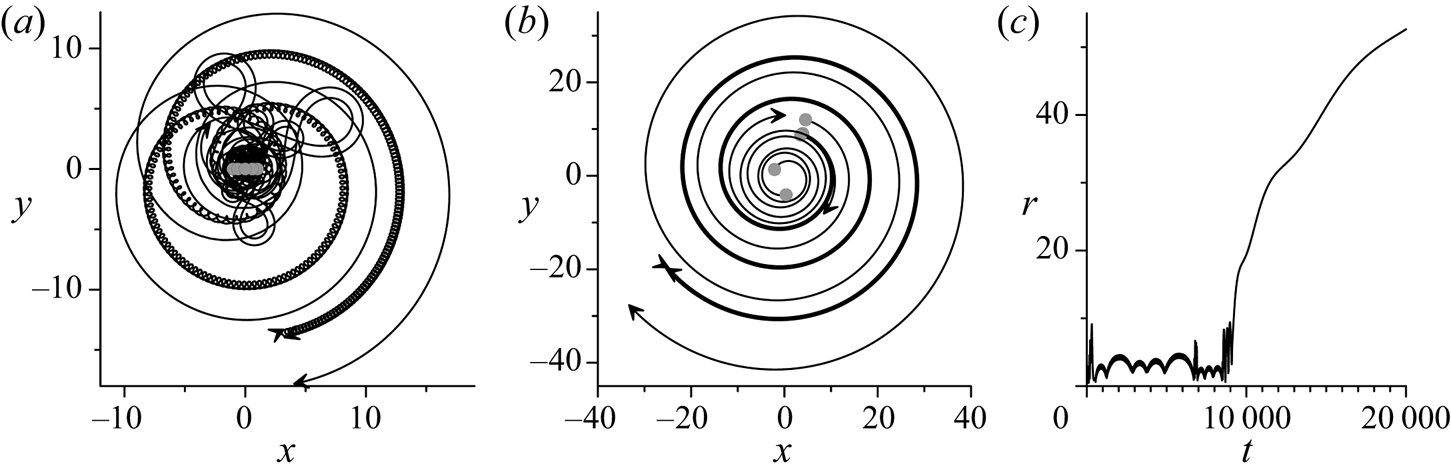
 $\delta = -0.8$ the necessary condition for scattering (2.6) is satisfied if a pair is formed by any two vortices with identical strengths. After loss of symmetry, the vortex ensemble first undergoes the stage of chaotic motion. Then two closely located vortices pair and, together with the three remaining vortices, participate in the expansion/convergence process (figure 13a,c). The final stage of the scattering starts at
 $t\approx 9500$ (figure 13b,c). Performing the best fit procedure, we found that in the interval
 $9500 \le t \le 20\;000$ the distances between the groups grow practically as the square root of time.
Complete scattering of four groups  $(\alpha ,\alpha ),\beta ,\beta ,\gamma $ emerged from a centrally symmetric collinear configuration of five vortices with
 $\alpha = \beta = -0.8,\;\gamma = 1$ and
 $\; \varphi _0 = 0,\;q_0 = 0.6$. Trajectories of absolute motion at (a)
 $0 \le t \le 2100$ and (b)
 $9500 \le t \le 20\,000$. (c) Maximal intervortex separation vs time. In (a,b), notations as in figure 11.

8. Group scattering of a large number of vortices with a random distribution of strengths
The total number of variants for splitting of N vortices into K groups  $(1 \le K \le N)$ exceed 10N already at
 $N \ge 61$; this can be calculated using the Bell numbers (Bell Reference Bell1938). If not all strengths have the same sign, one may anticipate that the necessary condition for group scattering (2.6) will be satisfied with good accuracy in a number of various scenarios where splitting can lead to expansion of an initially compact vortex configuration. To examine this hypothesis, a numerical experiment was carried out (figure 14). 1009 vortices were placed in the nodes of a square grid, which fall inside a circle of radius 8. The strengths of the vortices were chosen to be randomly distributed in the range (−1, 1).
Space distribution of 1009 vortices with random strengths uniformly distributed in the interval  $(-1,1)$, initially placed inside a circle (solid line in the first frame) centred at
 $(0,0)$ of radius 8 at (a)
 $t = 10^2$, (b)
 $t = 6 \times 10^4$, (c)
 $t = 3 \times 10^5$ and (d)
 $t = 2.4 \times 10^6$. Vortices with positive (negative) strength are marked with a plus sign (empty circle), whose size symbolizes the relative absolute value of the strength. The dashed circle whose centre (bold cross) is the centre of vorticity
 $(4.35,-0.29)$ encloses half of the vortices participating in the simulation.

Initially, the almost circular cloud of vortices loses its shape and begins to spread in space. This process akin to molecular diffusion is accompanied by emission of small groups, mainly vortex pairs, which have near-zero circulation. The area of the vortex cloud and the distances between separated groups grow with time, but the cloud shape does not undergo any qualitatively significant changes. This behaviour is characteristic of self-similarity (see simplest examples in §§ 5 and 7). Figure 14 shows the main part (approximately 95 %) of the vortex cloud at different times. Trajectories of the absolute motion of some vortices are shown in figure 15.
Absolute trajectories of four individual vortices; the size of the square is  $6000 \times 6000$ (in non-dimensional units), as in panel (d) in figure 14.

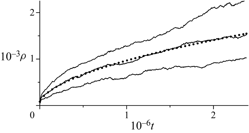
In figure 16, the rate of scattering is illustrated by the behaviour of quartiles (25 %, 50 % and 75 %) in the ordered distribution of distances from individual vortices to the centre of vorticity. A quartile, by definition, gives the radius of a circle enclosing 25 %, 50 % or 75 % of vortices. These graphs, therefore, characterize the mean intergroup separations, or in other words, the size of the cloud. Both the median and the interquartile range (the difference between the third and first quartiles) in general increase according to a power law  $(1 + \tau t)^\kappa $. The best fit of the median by a power function gives
 $\kappa \approx 0.545$ (dotted line in figure 16). This is quite close to
 $\kappa = 0.5$ characterizing self-similar expansion, i.e. the area of the vortex cloud grows almost linearly with time. Note that this result is in good agreement with that by Kizner, Khvoles & Kessler (Reference Kizner, Khvoles and Kessler2010), who showed analytically that the size of a vorticity patch during viscous self-similar expansion increases according to the square-root law. In our experiment, after
 $2.4 \times 10^6$ units of time, the area of the cloud increased approximately by 105 times. During the scattering, stirring and regrouping take place, so the asymptotically self-similar process is maintained due to the existence of a large number of various variants of splitting into groups.
Radius  $\rho (t)$ of circles enclosing 25 %, 50 % and 75 % of vortices (from bottom to top). Dotted line, the best-fit power function
 $\rho (t)\approx 82(1 + 0.00009t)^{0.545}$ for the 50 % circle.

9. Conclusion
We introduced the invariant function of the relative motion of N point vortices, which is a combination of four conserved quantities (interaction energy, the angular and two components of the linear momenta) and can be expressed through 2(N−2) independent phase variables. The isolines of the invariant function are phase trajectories of the relative motion, which is determined by the changes in the geometry of the vortex configuration during the evolution. Stationary points of the invariant function represent vortex equilibria, while the type of these points (a centre or a saddle point) determines the nonlinear stability of the corresponding relative equilibrium.
Singular points of the invariant function are related to scattering of the point vortices. Some of them are related to emission of some groups of the vortices with zero total circulation, and others, to complete scattering. We formulated a general necessary condition for group scattering of N vortices, that is for clustering of the ensemble into K groups that move apart and asymptotically (at large times) become independent.
Possible mechanisms of group scattering are elucidated via consideration of the evolution of a small number of vortices. At N = 3 and N = 4, 5 (provided that the central symmetry is kept) the invariant function depends on two variables only, which significantly simplifies understanding of the motion and analysis of the nonlinear stability of relative equilibria. Topologically (in the phase space), some of the singular points are centres, but when the necessary condition for scattering is fulfilled, they become nodes that attract phase trajectories located entirely within some finite domain. The boundaries of this domain of scattering (or emission of a dipole) are fragments of separatrices that pass through saddle points of the invariant function. When the point corresponding to the initial configuration lies on the singular curve R = 0, the well-known self-similar extension or collapse takes place. In the rest of the domain, the asymptotic-scattering (but not collapse) trajectories originate. Emission of dipole takes place only from phase trajectories which asymptotically approach the singular point where the relative distance between vortices formed a dipole tends to zero. When neither scattering nor emission is possible, at R = 0, periodic absolute motion is carried out, which consists of stages of expansion and convergence of vortices. Evolution at small values of L and/or R has a similar feature (but without strict periodicity) and occurs with sufficiently large expansion/convergence amplitudes. The expansion phase prevails in time during such a motion.
The mechanisms discussed above can also lead to a permanent expansion of a vortex configuration at N > 3, when the necessary condition for group scattering is satisfied. The simplest examples of the emission of two and three vortices and of complete scattering of three and four groups of vortices have been discussed in § 7 for N = 5.
In the case of a large number of vortices with strengths of different signs and values, numerous variants of splitting into groups of vortices exist. In many of them either  $L_G$ is almost zero (which makes possible of asymptotic group scattering), or the group analogue of the invariant M nearly vanishes (which facilitates abrupt expansion/convergence cycles). This leads to the increase in size of an initially compact vortex cloud; its area grows almost linearly with time. This is in good agreement with the analytical results obtained for self-similar motion of the point vortices in ideal fluid (Newton Reference Newton2001; Aref Reference Aref2010) and for viscous self-similar expansion of the vorticity patches (Kizner et al. Reference Kizner, Khvoles and Kessler2010).
Acknowledgements
The author is grateful to Z. Kizner for helpful discussions and comments on the manuscript. Thanks go to the anonymous reviewer for numerous suggestions that helped improve the article. This research was partially supported by the Mexican National Researchers System (SNI).
Declaration of interests
The author reports no conflict of interest.