2.1. Philosophy of the inlet condition

The key idea for the coupling between Temp-DNS and Spat-DNS is to use the former to generate planes of three-dimensional velocity fluctuations of HIT, $u_i^{(\textit{HIT})}$ , which are to be advected into the inlet of Spat-DNS at a constant convection velocity, $U_{\infty }$ . The relevance of considering these velocity fluctuations instead of numerical noise is threefold: (i) it allows for accurately controlling several properties of the inlet condition, such as the magnitude of turbulent kinetic energy, $k=\overline {u_i^{\prime}u_i^{\prime}}/2$ , the integral length scale, $L$ , or the r.m.s. of vorticity, $\omega '=({\overline {\omega _i^{\prime}\omega _i^{\prime}}})^{1/2}$ ; (ii) the fluctuations imposed are a solution of the NSEs, and (iii) there is a temporal-correlation between different time instants of the inlet condition. Moreover, the inlet flow fluctuations are isotropic. The prime, $(\boldsymbol{\cdot })'$ , represents the fluctuating part of the variable, according to the Reynolds decomposition, e.g. $u_i = \overline {u_i} + u_i^{\prime}$ . To maximise the potential of this approach, the time per iteration, $\varDelta t$ , as well as the grid cell size are kept equal on both Temp-DNS and Spat-DNS, such that no interpolation between fields of different codes is required.

In general, for the sake of creating spatially evolving TTIs, two simulations with different turbulent properties are run using Temp-DNS, HIT $i$ and HIT $j$ . At every time instant, the central velocity fields are imposed at the inlet of the Spat-DNS, alongside a convection velocity, $U_{\infty }$ , as depicted schematically in figure 1. Specifically, the inlet plane of Spat-DNS consists of an outer part of HIT $i$ and an inner region of HIT $j$ . Therefore, this plane has the same dimension as any of the central planes provided by the Temp-DNS code. Notice that the naming inner/outer, which shall be used throughout this work, is only a convention to differentiate between the two layers, and has no implicit physical mechanism of one layer confining the other, since the boundary condition in the normalwise direction is periodic. Finally, a passive scalar profile, $\phi$ , is added, which is used for identifying the TTI (as discussed in § 3).

2.2. Parametric study

In essence, the idea behind the parametric study is to modify independently both small- and large-scale parameters that we can accurately control/impose. Ultimately, we will be able to assess their influence on the overall flow development. In practice, we consider, initially, the integral length scale, $L$ , and vorticity fluctuations, $\omega '$ , for representing the large and small scales, respectively. With these two parameters, the minimum number of different homogeneous isotropic turbulence combinations we can create is 4 (large and low $L$ , each with large and low $\omega '$ , respectively). Concerning the details of these temporal simulations, all used a total number of $N^3 = 1024^3$ collocation points, with a kinematic viscosity value of $\nu = 0.0013$ . As aforementioned, the goal of these HIT simulations is to provide a range of different parameters, such as the velocity r.m.s., $u' = (\overline {u'^2})^{1/2}$ , the longitudinal integral length scale $L_{11}$ , vorticity r.m.s., $\omega '$ , and the Taylor-based Reynolds number, ${Re}_{\lambda } = u' \lambda / \nu$ , where $\lambda = ( 15 \nu \overline {u'^2} /\varepsilon )^{1/2}$ is the Taylor microscale. Table 1 describes the main physical parameters of the four HIT simulations, where the following notation was employed: $H$ represents a DNS of HIT, and the subscripts $L$ or $l$ , $\unicode{x1D6FA}$ or $\omega$ and $U$ or $u$ denote a (relatively) large or small magnitude of the integral length scale, vorticity fluctuations and velocity fluctuations, respectively. For example, ${H}_{L\omega u}$ refers to a HIT simulation with large integral length scale, and small vorticity and velocity fluctuations.

Table 1.

Parameters of each HIT simulation: wavenumber of maximum forcing, ${k}_p$ , longitudinal integral length scale, $L_{11}$ , resolution ${k}_{\textit{max}}\eta$ , Taylor-based Reynolds number, ${Re}_{\lambda }$ , root-mean-square vorticity $\omega '\equiv ({\varepsilon /\nu })^{1/2}$ and root-mean-square velocity $u'\equiv ({\overline {u'^2}})^{1/2}$ .

Essentially, we can pair the HIT simulations by magnitude of integral length scale, or r.m.s. of vorticity. Here, ${H}_{L\omega u}$ and ${H}_{L\unicode{x1D6FA} U}$ have similar (large) integral length scale, but varying vorticity fluctuations, while ${H}_{L\unicode{x1D6FA} U}$ and ${H}_{l\unicode{x1D6FA} U}$ have similar $\omega '$ , but different values of $L_{11}$ . The resolution is always ${k}_{\textit{max}}\eta \gtrsim 1$ and the Taylor-based Reynolds number is $146\lesssim {Re}_{\lambda }\lesssim 296$ , which is sufficiently high to assess the possible existence of universality results. Noticeably, there is some dependence of $u'$ and ${Re}_{\lambda }$ on the aforementioned parameters. Indeed, since the number of collocation points and the value of the kinematic viscosity need to be the same in all simulations, we have manipulated the magnitude of the input forcing power $P$ , the peak location of this forcing ${k}_p$ , as well as the resolution ${k}_{\textit{max}} \eta$ (however, making sure it is at least ${k}_{\textit{max}} \eta = 1$ ) to change physically relevant parameters. The selection of these is based on a few simple equations. By using the fact that in statistically stationary conditions, the power input of the forcing is equal to the viscous dissipation rate, $P = \varepsilon$ , and using the definition of the non-dimensional dissipation, $C_{\varepsilon }$ ,

(2.1) \begin{align} \varepsilon = C_{\varepsilon } \frac {u^{\prime 3}}{L_{11}}, \end{align}

together with the definition of the Taylor-based Reynolds number, and the Kolmogorov microscale $\eta = ( \nu ^3 /\varepsilon )^{1/4}$ , one arrives at expressions for the maximum attainable Reynolds number (for given integral length scale $L_{11}$ and resolution ${k}_{\textit{max}} \eta$ )

(2.2) \begin{equation} {Re}_{\lambda } = \sqrt {15} \left ( \frac {L_{11}}{C_{\varepsilon }} \right )^{2/3} \left ( \frac {N}{2} \right )^{2/3} \left ( \frac {A}{{k}_{\textit{max}} \eta } \right )^{2/3}, \end{equation}

where $A = 2/3$ (fully de-aliased simulations). In the estimation, we have used $C_{\varepsilon } = 0.44$ for forced HIT (Pope Reference Pope2000). The kinematic viscosity $\nu$ and forcing power $P$ that correspond to this condition are related by

(2.3) \begin{equation} P = \nu ^3 \left ( \frac {A}{{k}_{\textit{max}}\eta } \frac {N}{2} \right )^{4}, \end{equation}

and the corresponding resolution is

(2.4) \begin{equation} {k}_{\textit{max}} \eta = A \left ( \frac {N}{2} \right ) \left ( \frac {\nu ^3}{P} \right )^{1/4}. \end{equation}

Noticeably, (2.2) can also be written as a function of $\nu$ and $P$ ,

(2.5) \begin{equation} {Re}_{\lambda } = \sqrt {15} \left ( \frac {L_{11}}{C_{\varepsilon }} \right )^{2/3} \left ( \frac {P^{1/3}}{\nu } \right )^{1/2}. \end{equation}

These relations are remarkably accurate in predicting the flow properties, given a certain input list of parameters, and allow for an unprecedented level of control over the turbulent properties of spatially evolving TTIs without mean shear.

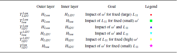
The resultant six different spatially evolving TTI simulations use the possible combinations of the aforementioned types of HIT. The domain size is $(L_x,L_y,L_z)=(4\pi ,2\pi ,2\pi )$ and the corresponding grid is $N_x\times N_y\times N_z=2048\times 1024\times 1024$ . This novel approach allows for varying $N_x$ , but it restricts $N_y$ and $N_z$ (as these shall be consistent with the grid of Temp-DNS simulations). A convection velocity of $U_{\infty }=5$ was selected, which ensured that the turbulence intensity, $T_u=u'/U_{\infty }$ , would not exceed unity. Therefore, it also ensures that there is, on average, no backflow at the inlet, since one has $\min (u)=U_{\infty }-u'\gt 0$ . Moreover, before imposing inlet velocity fluctuations, we ensure a constant $U_{\infty }$ velocity in the streamwise direction at all grid points. Also, the statistics are not accumulated until the flow has crossed one full box length.

A summary is presented in table 2. In this case, ${T}$ represents a DNS of TTIs and the subscripts (superscripts) refer to the inner (outer) layer. Specifically, as before, $L$ or $l$ , $\unicode{x1D6FA}$ or $\omega$ and $U$ or $u$ denote a (relatively) large or small magnitude of the integral length scale, vorticity fluctuations and velocity fluctuations, respectively. For instance, ${T}_{L\unicode{x1D6FA} U}^{L\omega u}$ indicates a TTI simulation with fixed large integral length scale, and small (large) vorticity and velocity fluctuations in the outer (inner) layer. Notice, however, that whereas for the integral length scale and vorticity fluctuations one has only two possible quantitative values, i.e. ${\sim} 0.9$ and ${\sim} 0.5$ for $L_{11}$ , and ${\sim} 150$ and ${\sim} 65$ for $\omega '$ (cf. table 1), the velocity fluctuations can have slightly different values within the same low/high magnitude states, e.g. ${\sim} 1.8$ and $ {\sim} 2.3$ shall be considered as low magnitude, but they differ by approximately $25\,\%$ . Whenever pertinent to explain the dynamics, the small difference that exists shall be pointed out.

Table 2.

Combinations of HIT simulations to produce spatially-evolving TTIs. The legend refers to the colour of the curves.

Simulations ${T}_{L\unicode{x1D6FA} U}^{L\omega u}$ and ${T}_{l\unicode{x1D6FA} U}^{l\omega u}$ keep the integral length scale across layers constant (being large and small, respectively), and change $\omega '$ , while ${T}_{l\omega u}^{L\omega u}$ and ${T}_{l\unicode{x1D6FA} U}^{L\unicode{x1D6FA} U}$ assess the contrary scenario. In contrast, ${T}_{l\unicode{x1D6FA} U}^{L\omega u}$ and ${T}_{l\omega u}^{L\unicode{x1D6FA} U}$ do not have fixed parameters, but shall be relevant for comparison with the previous cases. We can summarise the main parameters of the simulations in the three-dimensional $L_{11}-T_u-\omega '$ parametric space, where it is insightful to consider the ratios of these quantities from outer to inner layers, e.g. $T_u^{({\textit{Outer}})}/T_u^{({\textit{Inner}})}$ as the variables. Naturally, we can project it into the two-dimensional $L_{11}{-}T_u$ and $\omega '{-}T_u$ maps, which allows for simplifying the analysis. All three spaces are depicted in figure 2.

Figure 2.

Parametric space (a) $L_{11}{-}T_u{-}\omega '$ and respective two-dimensional projections (b) $L_{11}{-}T_u$ , and (c) $\omega '{-}T_u$ . The grey regions correspond to regions with the ratios $L_{11}^{({\textit{Outer}})}/L_{11}^{({\textit{Inner}})}$ , $T_u^{({\textit{Outer}})}/T_u^{({\textit{Inner}})}$ or $\omega '^{({\textit{Outer}})}/\omega '^{({\textit{Inner}})}$ equal to $1\pm 0.1$ , and hence are considered as roughly constant. Notice that the Taylor-based Reynolds number also varies, as shown in table 1, but it encompasses effects of both large and small scales, being completely dependent of the other parameters.

First, the $L_{11}{-}T_u{-}\omega '$ space (figure 2 a) shows that we cover a large portion of the available parametric space. More precisely, in the $L_{11}{-}T_u$ map (figure 2 b), the existence of simulations representing almost three of the four possible quadrants, for an origin located at $(1,1)$ , is highlighted. Namely, ${T}_{l\omega u}^{L\omega u}$ , ${T}_{l\omega u}^{L\unicode{x1D6FA} U}$ and ${T}_{l\unicode{x1D6FA} U}^{L\unicode{x1D6FA} U}$ present ${L_{11}^{({\textit{Outer}})}}/{L_{11}^{({\textit{Inner}})}}\!\gt \!1$ and $T_u^{({\textit{Outer}})}/T_u^{({\textit{Inner}})}\!\gt \!1$ (first quadrant), ${T}_{l\unicode{x1D6FA} U}^{L\omega u}$ has $L_{11}^{({\textit{Outer}})}/L_{11}^{({\textit{Inner}})}\!\gt \!1$ and $T_u^{({\textit{Outer}})}/T_u^{({\textit{Inner}})}\!\lt \!1$ (second quadrant), while ${T}_{L\unicode{x1D6FA} U}^{L\omega u}$ and ${T}_{l\unicode{x1D6FA} U}^{l\omega u}$ showcase $L_{11}^{({\textit{Outer}})}/L_{11}^{({\textit{Inner}})}\!\sim \! 1$ and $T_u^{({\textit{Outer}})}/ T_u^{({\textit{Inner}})}\!\lt \!1$ (at the border between second and third quadrants). It is worth remarking that ${T}_{L\unicode{x1D6FA} U}^{L\omega u}$ and ${T}_{l\unicode{x1D6FA} U}^{l\omega u}$ , as well as ${T}_{l\omega u}^{L\omega u}$ and ${T}_{l\unicode{x1D6FA} U}^{L\unicode{x1D6FA} U}$ are almost superimposed, despite the different magnitude of integral length scales or $T_u$ . Notice that the portion of the $L_{11}{-}T_u$ map with $L_{11}^{({\textit{Outer}})}/L_{11}^{({\textit{Inner}})}\!\lt \!1$ was omitted for the sake of simplification. Regarding the $\omega '{-}T_u$ parametric space (figure 2 c), we can distinguish between ${T}_{l\omega u}^{L\unicode{x1D6FA} U}$ , with $\omega '^{({\textit{Outer}})}/\omega '^{({\textit{Inner}})}\!\gt \!1$ and $T_u^{({\textit{Outer}})}/T_u^{({\textit{Inner}})}\!\gt \!1$ (first quadrant), the group ${T}_{L\unicode{x1D6FA} U}^{L\omega u}$ , ${T}_{l\unicode{x1D6FA} U}^{L\omega u}$ and ${T}_{l\unicode{x1D6FA} U}^{l\omega u}$ showcasing $\omega '^{({\textit{Outer}})}/\omega '^{({\textit{Inner}})}\!\lt \!1$ and $T_u^{({\textit{Outer}})}/T_u^{({\textit{Inner}})}\!\lt \!1$ (third quadrant), and finally ${T}_{l\omega u}^{L\omega u}$ and ${T}_{l\unicode{x1D6FA} U}^{L\unicode{x1D6FA} U}$ with $\omega '^{({\textit{Outer}})}/\omega '^{({\textit{Inner}})}\!\sim \! 1$ and $T_u^{({\textit{Outer}})}/T_u^{({\textit{Inner}})}\!\gt \!1$ (at the border between fourth and first quadrants). These positions shall be important when characterising the dynamics of the flow evolution in § 4.1.

4.1. Passive scalar-related quantities

Finally, looking at the passive scalar field is also pertinent. Indeed, as aforementioned, this quantity will be used for identifying the TTIs. Additionally, it allows for understanding some trends as to which is the dominant layer. Figure 9 depicts both the average passive scalar, $\overline {\phi }^f$ , and its variance, $\overline {\phi '^2}^f$ .

Figure 9.

Contours of $\overline {\phi }$ (upper) and $\overline {\phi '^2}$ (lower) for simulations (a) ${T}_{L\unicode{x1D6FA} U}^{L\omega u}$ , (b) ${T}_{l\omega u}^{L\omega u}$ , (c) ${T}_{l\unicode{x1D6FA} U}^{L\omega u}$ , (d) ${T}_{l\omega u}^{L\unicode{x1D6FA} U}$ , (e) ${T}_{l\unicode{x1D6FA} U}^{L\unicode{x1D6FA} U}$ and ( f) ${T}_{l\unicode{x1D6FA} U}^{l\omega u}$ . The dashed lines highlight the initial separation between outer and inner turbulent regions. The passive scalar field scale was restricted to the interval $[0.4;0.6]$ for the sake of highlighting the region with $\phi =0.5$ .

The passive scalar spreads with streamwise distance. If we look at the distance between white and black regions of the upper semiplanes, i.e. $0.4\leqslant \phi \leqslant 0.6$ , we observe that, closer to the outlet, this distance is much greater for ${T}_{l\omega u}^{L\unicode{x1D6FA} U}$ or ${T}_{l\unicode{x1D6FA} U}^{L\unicode{x1D6FA} U}$ than for ${T}_{l\omega u}^{L\omega u}$ or ${T}^{l\omega u}_{l\unicode{x1D6FA} U}$ . Such results suggest that the combination, for example, of ${H}_{L\unicode{x1D6FA} U}$ with ${H}_{l\omega u}$ enhances the turbulent diffusivity of passive scalar when compared with that of ${H}_{L\omega u}$ and ${H}_{l\omega u}$ . This is linked to the value of $\phi$ at the centreline, $\phi _c$ , since the higher the diffusion, the lower the passive scalar mean value at the middle of the domain. In other words, given that the total domain quantity of $\phi$ is approximately constant, when the outer region has an increased value of scalar concentration, then its presence on the inner part should decrease accordingly. The evolution of $\phi _c$ with $x/H$ is shown in figure 10(a). Clearly, the preceding observation is more directly proved here: ${T}_{l\omega u}^{L\unicode{x1D6FA} U}$ and ${T}_{l\unicode{x1D6FA} U}^{L\unicode{x1D6FA} U}$ have a faster decrease of the centreline value, possibly due to the presence of an outer layer with a higher energy and ${Re}_{\lambda }$ , i.e. ${H}_{L\unicode{x1D6FA} U}$ . In contrast, ${T}_{l\omega u}^{L\omega u}$ and ${T}^{l\omega u}_{l\unicode{x1D6FA} U}$ have a slower decay. Nevertheless, interestingly, all profiles, apart from ${T}_{L\unicode{x1D6FA} U}^{L\omega u}$ , seem to follow a power law of the type $(x/H)^{-\beta }$ , with $\beta \sim 0.3$ , at the end of the domain. For the sake of comparison, and even though a quantitative assessment of $\beta$ is not under analysis, the theoretical exponents for axisymmetric jets would be $\beta =1$ , while for planar jets or wakes, one derives $\beta =0.5$ (Schlichting & Gersten Reference Schlichting and Gersten2016). The lack of mean shear in this flow might explain the slower decay rate, when compared with the aforementioned canonical cases. The two most important takeaways are that, on the one hand, different layers will induce dissimilar passive scalar centreline evolutions, confirming the utmost importance of turbulent properties in dictating the dynamics of $\phi$ , and, consequently, of TTIs. On the other hand, in the long term, i.e. for high enough $x/H$ , almost all curves tend to an asymptotic similar decay rate. There, homogenisation has largely taken place and perhaps the differences between layers are not so dramatic as to affect the passive scalar differently.

So far, the concentration of $\phi$ and its value at the centreline confirmed that the passive scalar is greatly influenced by the characteristics of each layer. However, it would be beneficial to find a metric that could provide something related to a direction, or trend, that could help in understanding the spreading of each turbulent region, ultimately connected to the exchanges occurring at the TTI, quantitatively. Focussing on the passive scalar variance yields great insight on this topic. Recalling, its contours are shown in the lower semiplanes of figure 9, for all six simulations. The maps of this quantity are similar for all simulations, with a peak of $\overline {\phi '^2}$ at $x/H\approx 0.5$ . Additionally, we can look at the direction of the maximum passive scalar variance for each $x/H$ . In some cases, it is tilted inwards, outwards or stays approximately horizontal (neutral), which clearly introduces a degree of freedom associated with the $y$ direction. We can more systematically compare these trends by defining a thickness based on the maximum passive scalar variance,

(4.4) \begin{equation} \delta _{{var}(\phi )}:\overline {\phi '^2}\left(x/H,y/H=\delta _{{var}(\phi )}/H\right)=\max \big(\overline {{\phi '}^2}\big). \end{equation}

At the inlet, the simulations should present $\delta _{{var}(\phi )}/H\approx 0.5$ and if this value decreases (increases), the physical interpretation is that the outer (inner) layer is prevailing. That occurs since $\overline {\phi '^2}$ is, analogously to $\overline {u'^2}$ , a measure of an energy. Therefore, if some external property is modifying the direction of maximum passive scalar energy, it surely is prescribing its properties. The evolution of $\delta _{{var}(\phi )}/H$ is summarised in figure 10(b).

Figure 10.

Streamwise evolution of (a) the passive scalar concentration at the centreline ( $y=0$ ), $\phi _c$ , and (b) the half-width thickness based on the maximum passive scalar variance, for all simulations.

Despite the slight oscillatory behaviour ( $\delta _{{var}(\phi )}$ is highly sensitive to small variations, but we are mostly interested in obtaining qualitative trends), it is clear that there are three different possibilities. In some cases, $\delta _{{var}(\phi )}/H$ grows, e.g. ${T}^{L\omega u}_{L\unicode{x1D6FA} U}$ and ${T}^{l\omega u}_{l\unicode{x1D6FA} U}$ , in others, it diminishes, e.g. ${T}_{l\omega u}^{L\omega u}$ , ${T}_{l\omega u}^{L\unicode{x1D6FA} U}$ , ${T}_{l\unicode{x1D6FA} U}^{L\unicode{x1D6FA} U}$ , or even stays approximately neutral, e.g. ${T}_{l\unicode{x1D6FA} U}^{L\omega u}$ . We can associate each of the layers’ properties (recalling table 1) with these trends, in an attempt to finally provide a general framework for the impact of $\omega '$ , $u'$ and $L_{11}$ on the spreading of passive scalar and TTIs. First, for the simpler cases, i.e. when we have fewer parameters varying, we can highlight some empirical observations. Namely, for ${T}_{l\omega u}^{L\omega u}$ and ${T}_{l\unicode{x1D6FA} U}^{L\unicode{x1D6FA} U}$ , even though the levels of $\omega '$ across the layers do not change, we see a trend on $\delta _{{var}(\phi )}$ . This means that this quantity alone is not capable of dictating the dynamics of $\delta _{{var}(\phi )}$ (otherwise a neutral behaviour would have been observed). From it, one can suggest that the r.m.s. of vorticity does not influence considerably the half-width thickness based on the maximum passive scalar variance. It may even be possible to go one step further and suggest that the spreading of turbulence across TTIs is not directly related to small-scale quantities. In these cases, since the outer layer is prevailing, we can say that either $L_{11}$ or $u'$ are relevant in imposing the orientation, since both of them are greater for the outer region. Thereupon, if we take this rationale further, assuming that $\omega '$ does not directly influence the trends, the evolution of $\delta _{{var}(\phi )}$ for ${T}_{L\unicode{x1D6FA} U}^{L\omega u}$ and ${T}_{l \unicode{x1D6FA} U}^{l\omega u}$ , which have a constant $L_{11}$ (cf. figures 8 a and 8 f), leads to the conclusion that, for these cases, the growth of $\delta _{{var}(\phi )}/H$ is totally dependent on $u'$ . Finally, the two simulations with all parameters varying suggest the following: for ${T}_{l\omega u}^{L\unicode{x1D6FA} U}$ , both $L_{11}$ and $u'$ are larger in the same layer; therefore, both properties shall work for the end result, i.e. to make the outer layer dominate, which induces a strongly inwards motion. However, ${T}_{l\unicode{x1D6FA} U}^{L\omega u}$ has a slightly higher $u'$ on the inner region, which would make this layer dominate, and a slightly lower $L_{11}$ , which would induce the outer layer to prevail. The end result is a neutral, not well-defined trend, as shown. Recalling the work of Tordella & Iovieno (Reference Tordella and Iovieno2006) on shearless turbulence mixing layers is pertinent. There, it is observed that, when the gradient in turbulent kinetic energy and integral length scale from one region to another have the same sign (i.e. either both are increasing or decreasing in the same direction), then there is a greater transport (in terms of kinetic energy) than when these gradients have different signs, i.e. are acting against each other. Here, an analogous situation occurs, however, for the passive scalar variance, ultimately connected to the spreading of each turbulent region in communication through the TTIs: for cases when $T_u^{({\textit{Outer}})}/T_u^{({\textit{Inner}})}\!\gt \!1$ and $L_{11}^{({\textit{Outer}})}/L_{11}^{({\textit{Inner}})}\!\gt \!1$ , there is a prevalence of the outer layer, whereas when $T_u^{({\textit{Outer}})}/T_u^{({\textit{Inner}})}\!\lt \!1$ and $L_{11}^{({\textit{Outer}})}/L_{11}^{({\textit{Inner}})}\!\lt \!1$ , the inner region dominates, both of which correspond to the situations where the transport is maximised. The case where $T_u^{({\textit{Outer}})}/T_u^{({\textit{Inner}})}\!\gt \!1$ and $L_{11}^{({\textit{Outer}})}/L_{11}^{({\textit{Inner}})}\!\lt \!1$ leads to an ill-defined behaviour, which is translated through the existence of contrary gradients. All this can be linked to the maps presented in figure 2. Indeed, one can suggest that, on the one hand, if we are located in the first quadrant of the $L_{11}{-}T_u$ map (figure 2 b), then the outer layer shall prevail. In opposition, if we are located in the third quadrant, the inner layer will prevail. The even quadrants reflect a not well-defined trend, ultimately concomitant to the fact that $T_u$ and $L_{11}$ are acting against each other. On the other hand, since $\omega '$ does not play a significant role on the spreading, the $\omega '{-}T_u$ map (figure 2 c) does not convey a clear trend. Eventually, we suggest that, more important than the values of $T_u$ or $L_{11}$ themselves, is the ratio from outer to inner, since some values for the various TTIs cases studied are located in the same coordinates on these maps, and they present similar trends.

5.1. Quasi-universality of small-scale dynamics

We now move into the detailed analysis of quantities associated with the velocity/vorticity fields. As such, figure 14 shows the conditional statistics of enstrophy and rate-of-strain magnitude, $\omega _i\omega _i$ and $s_{ij}s_{ij}$ , the most relevant small-scales quantities, for ${T}_{l\omega u}^{L\omega u}$ , ${T}_{l\omega u}^{L\unicode{x1D6FA} U}$ and ${T}_{l\unicode{x1D6FA} U}^{l\omega u}$ . Here, all curves were rescaled by a constant value corresponding to the turbulent core value of enstrophy or rate-of-strain magnitude of the slab closest to the inlet. From the two turbulent core regions, outer and inner, we choose the one with the highest magnitude of $\omega _i\omega _i$ or $s_{ij}s_{ij}$ . In terms of notation, we denote these values by $\langle \boldsymbol{\cdot }\rangle _T^{{(inlet)}}$ .

Figure 14.

Conditional statistics of (a,c,e) enstrophy, $\langle \omega _i\omega _i\rangle _I$ , and (b,d,f) rate-of-strain magnitude, $\langle s_{ij}s_{ij}\rangle _I$ , for ${T}_{l\omega u}^{L\omega u}$ , ${T}_{l\omega u}^{L\unicode{x1D6FA} U}$ and ${T}_{l\unicode{x1D6FA} U}^{l\omega u}$ , respectively. Light/dark curves represent locations closer to the inlet/outlet of the domain, respectively.

Each of the three simulations were meticulously chosen to represent one of three distinct groups which showcase different qualitative evolutions of enstrophy or rate-of-strain magnitude: (i) when the levels of $\omega _i\omega _i$ and $s_{ij}s_{ij}$ are similar in both layers (as in ${T}_{l\omega u}^{L\omega u}$ and ${T}_{l\unicode{x1D6FA} U}^{L\unicode{x1D6FA} U}$ , cf. figures 6 b and 6 e for $\omega '$ ); (ii) when the outer layer presents a higher magnitude of $\omega _i\omega _i$ and $s_{ij}s_{ij}$ (as observable in ${T}_{l\omega u}^{L\unicode{x1D6FA} U}$ , cf. figure 6 d), or (iii) when the inner layer has a greater magnitude of the small-scale terms (as in ${T}_{L\unicode{x1D6FA} U}^{L\omega u}$ , ${T}_{l\unicode{x1D6FA} U}^{L\omega u}$ or ${T}_{l\unicode{x1D6FA} U}^{l\omega u}$ , cf. figures 6 a, 6 c and 6 f). There are several key aspects regarding the spatial evolution of these quantities. First of all, both enstrophy and strain present a decay with $x$ , as expected, since the forcing is only located at the inlet, and the turbulence decays freely afterwards. For ${T}_{l\omega u}^{L\omega u}$ , the enstrophy profiles depict two small bumps, i.e. peaks, on each side of the TTI, whose presence can be associated to an increased vorticity near the TTI. However, when the magnitudes of enstrophy are quite dissimilar (for instance, the curves closer to the inlet in figures 14 c and 14 e), we observe only one (clear) peak in the layer with the highest level of vorticity magnitude, which starts recalling what is qualitatively observed in TNTIs (Zecchetto & da Silva Reference Zecchetto and da Silva2021). Indeed, it is almost as if, in the limit of very dissimilar levels of enstrophy (vorticity r.m.s.) between two layers, $\omega '^{(i)}\ll \omega '^{(j)}$ , we would tend to a TNTI.

In terms of the rate-of-strain magnitude, we observe a peak at the interface ( $\langle y \rangle _I= 0$ ), regardless of the location, meaning that this interfacial region is dominated by a straining motion. Nevertheless, TNTIs do not exhibit a peak of $s_{ij}s_{ij}$ and it is certainly relevant to understand the cause for its appearance in this context. If we compare the conditional strain, $\langle s_{ij}s_{ij}\rangle _I$ , closer to the inlet for simulations ${T}_{l\omega u}^{L\omega u}$ and ${T}_{l\unicode{x1D6FA} U}^{l\omega u}$ , we observe that the peak of the former reaches a magnitude almost twice that of the value at the turbulent cores, and hence is important. Yet, for the latter simulation, the strain peak has a relatively small magnitude when compared with the turbulent core value of the inner region ( $\langle y\rangle _I\to \infty$ ). As the flow decays, the peak, even though decreasing its magnitude, becomes more dominant with respect to the turbulent core values, since the strain levels get closer, eventually tending to the state of ${T}_{l\omega u}^{L\omega u}$ . However, if we extend this argument in reverse, then as the difference in the two bulk rate-of-strain magnitudes increases, the local peak at the interface diminishes in importance until it becomes negligible, thereby recovering the phenomenology of a TNTI. All in all, we present this schematic that consists of: (i) a TNTI being a special case of the more general TTIs when the difference in the levels of $\omega '$ is taken ad extremum; and (ii) a TTI with similar levels of $\omega '$ in both turbulent regions being the asymptotic case to which the interfaces tend after a sufficiently long spatial decay.

The observation of peaks and valleys in the enstrophy and strain-rate magnitude motivates the use of a normalisation of the former by the local Kolmogorov microscales (Zecchetto & da Silva Reference Zecchetto and da Silva2021), $u_{\eta }\equiv (\nu \varepsilon )^{1/4}$ and $\eta$ . Dimensionally, it can be analytically expressed as $\langle \omega _i\omega _i\rangle _I/(\langle u_{\eta }\rangle _I/\langle \eta \rangle _I)^2$ . Notice that one can also interpret this normalisation as being the relation between enstrophy and the Kolmogorov time scale, $\tau _{\eta }\equiv \eta /u_{\eta }$ , yielding $\langle \omega _i\omega _i \rangle _I\langle \tau _{\eta }\rangle _I^2$ . Additionally, it is particularly useful (and equivalent) to understand it as a balance between the average enstrophy and (twice) the average rate of rate-of-strain magnitude, $\langle \omega _i\omega _i\rangle _I/\langle 2s_{ij}s_{ij} \rangle _I$ . These profiles are shown in figure 15 for all six simulations and at $x/H\in [0.5;0.6]$ .

Figure 15.

Conditional profiles of enstrophy normalised by local Kolmogorov microscales at $x/H\in [0.5;0.6]$ for ${T}_{L\unicode{x1D6FA} U}^{L\omega u}\!$ , ${T}_{l\omega u}^{L\omega u}\!$ , ${T}_{l\unicode{x1D6FA} u}^{L\omega u}\!$ , ${T}_{l\omega u}^{L\unicode{x1D6FA} U}\!$ , ${T}_{l\unicode{x1D6FA} U}^{L\unicode{x1D6FA} U}$ and ${T}_{l\unicode{x1D6FA} U}^{l \omega u}$ .

Qualitatively, all simulations present a similar double-peak curve, regardless of their different parameters. These shapes are in line with the results of Nakamura et al. (Reference Nakamura, Watanabe and Nagata2023) and Chen & Buxton (Reference Chen and Buxton2024). Since the strain has a peak close to the interface location (cf. figure 14 b, d, f; however, relatively less prominent the greater the vorticity magnitude difference), it will provoke a minimum on the Kolmogorov-normalised enstrophy profile near $\langle y\rangle _I=0$ . The visible valleys siding the strain peak will result from the bumps that were observed on the conditional enstrophy profiles (cf. figure 14 a, c, e). As we move towards the turbulent cores, $\langle y \rangle _I/\langle \eta \rangle _I\to \pm \infty$ , the normalisation tends to $1$ , which is a kinematic constraint for homogeneous flows (Tsinober Reference Tsinober2000; Zecchetto & da Silva Reference Zecchetto and da Silva2021). Nonetheless, the slightly different value can be attributed to the location of the slab, which is still close to the inlet and some adjustment to the initial condition could be taking place. In terms of the distance between these consecutive maxima, values in line with the results of Nakamura et al. (Reference Nakamura, Watanabe and Nagata2023) are obtained, i.e. $\langle y\rangle _I/\langle \eta \rangle _I\approx 6{-}7$ . This represents roughly half the value reported for this distance by Chen & Buxton (Reference Chen and Buxton2024). When comparing all curves, we notice two points of relevance. On the one hand, there exist curves which are almost superimposed, such as ${T}_{l\unicode{x1D6FA} U}^{L\omega u}$ and ${T}_{l\unicode{x1D6FA} U}^{l\omega u}$ , in spite of having completely different evolutions of the large-scale parameters (e.g. ${T}_{l\unicode{x1D6FA} U}^{L\omega u}$ has a gradient on $L_{11}$ , while ${T}_{l\unicode{x1D6FA} U}^{l\omega u}$ does not). This means that the large-scale parameters play no significant role on the local dynamics of TTIs. Yet, one cannot say the same about the small-scale quantities, such as $\omega '$ . Indeed, the magnitude of the peaks is precisely associated with how different are the levels of vorticity fluctuations. To show this, we evaluate the streamwise evolution of $\langle \omega _i\omega _i\rangle _I/(\langle u_{\eta } \rangle _I/\langle \eta \rangle _I)^2$ , as presented in figure 16, recalling that as the flow develops, the levels of enstrophy generically homogenise.

Figure 16.

Conditional profiles of enstrophy normalised by local Kolmogorov microscales at several streamwise locations for (a) ${T}_{l\omega u}^{L\omega u}$ , (b) ${T}_{l\omega u}^{L\unicode{x1D6FA} U}$ and (c) ${T}_{l\unicode{x1D6FA} U}^{l\omega u}$ . Light/dark curves represent locations closer to the inlet/outlet of the domain, respectively. The arrows point in the downstream direction.

Fundamentally, for ${T}_{l\omega u}^{L\omega u}$ , with similar (low) $\omega '$ levels on both sides, especially closer to the inlet, the curves are approximately invariant to the slab $x/H$ , and the peaks have similar magnitudes, i.e. $\langle \omega _i\omega _i \rangle _I/ \langle 2s_{ij}s_{ij}\rangle _I\approx {1.25}$ , which is well in agreement with the value obtained for TNTIs, $\langle \omega _i\omega _i \rangle _I/ \langle 2s_{ij}s_{ij}\rangle _I=1.248$ (Zecchetto & da Silva Reference Zecchetto and da Silva2021). For ${T}_{l\omega u}^{L\unicode{x1D6FA} U}$ , the inner region has an initial smaller $\omega '$ , inducing a diminished peak magnitude. Here, the impact of $x/H$ is non-negligible: as $x/H$ increases, the correspondent peak is slowly shifted upwards. This can be interpreted in light of the observations previously remarked: turbulence decays and tends to an homogeneous configuration, and we would eventually reach an asymptotic state similar to that of ${T}_{l\omega u}^{L\omega u}$ , where the magnitude of the peaks is similar, since both regions have comparable enstrophies. A mirrored case occurs for ${T}_{l \unicode{x1D6FA} U}^{l\omega u}$ , where it is the outer region with the lowest r.m.s. of vorticity. Here, the evolution of the peak magnitude corresponding to the outer layer is even clearer, since the levels of enstrophy on the slabs closer to the outlet are much more comparable (cf. figure 14 e). It has become clear how the only parameter differentiating all curves is how contrasting the levels of vorticity magnitude are on each layer, i.e. $\omega '^{{(\textit{Outer})}}/\omega '^{{(\textit{Inner})}}$ . This sustains the previous remark that neither the integral length scale, $L_{11}$ , nor the turbulence intensity, $T_u$ , both of which are large-scale properties, impact the dynamics of small-scale quantities near the TTIs.

Due to this quasi-universality, one may wonder about the flow structures near the TTIs. Figure 4(b) had already shown that the passive scalar correctly distinguishes zones with two different non-null vorticity magnitudes, but the inherent two-dimensionality and the use of $\sqrt {\omega _i\omega _i}$ , does not allow for a proper assessment of the eddies in close proximity to the TTI. In figure 17, we show a three-dimensional visualisation of rotational structures identified with a value of the second invariant of the velocity gradient tensor (VGT), $Q=4000$ (arbitrary units) for ${T}_{l\unicode{x1D6FA} U}^{l\omega u}$ and $x/H\in [0.4;0.8]$ . These are coloured by the passive scalar field, and are separated between those identified in the inner region (figure 17 a) and in the outer region (figure 17 b).

Figure 17.

Three-dimensional visualisation of the flow structures. The rotational eddies identified by the $Q=4000$ (arbitrary units) inside the (a) inner and (b) outer layers are coloured by the passive scalar concentration. The translucent surface corresponds to the TTI. The snapshot of an arbitrary time instant refers to simulation ${T}_{l\omega u}^{l\omega U}$ .

The vortices closer to the interface are (visually) tangent to the TTI. Despite not being as clear as in the case of TNTIs (da Silva, Dos Reis & Pereira Reference da Silva, Dos Reis and Pereira2011), the turbulent/turbulent interface does not cut a vortex in the normal direction. Moreover, the inner layer has a much higher density of eddies than the outer layer, which is in total agreement with the conditional enstrophy statistics of figure 14 and the inlet imposition (cf. table 2). Both these arguments ultimately support the quasi-universality previously sketched: on average, the eddies are tangent on both sides of the TTI, which induces a straining motion in between both, and a higher rotationality on either side of the interface. This is in line with the results of Kankanwadi & Buxton (Reference Kankanwadi and Buxton2022) pertaining the enhanced interface-normal rate-of-strain near TTIs, which is associated with a local anisotropy. In addition, the lesser density of eddies on one side yields a smaller magnitude of the normalised peak. Eventually, if there were no eddies in one of the regions (TNTI type of situation), we would recover a profile with a single maximum.

This whole discussion, strictly related to the connection between enstrophy and the strain-rate magnitude in the vicinity of TTIs, cannot be underestimated. Recalling the works of Buaria et al. (Reference Buaria, Pumir, Bodenschatz and Yeung2019, Reference Buaria, Pumir and Bodenschatz2020) on extreme velocity gradients is pertinent, as they have provided some insight on the relation between those variables, i.e. $\omega _i\omega _i$ and $s_{ij}s_{ij}$ . In particular, they found that whenever these quantities are much smaller than the average, they appear to be decorrelated, whereas if they are much larger, they present a power-law dependence, e.g. enstrophy conditioned on rate-of-strain magnitude grows linearly with it. It would be interesting to see if these observations hold in the inhomogeneous cases of turbulent/turbulent interfaces, where the premise $\langle \omega _i\omega _i\rangle _I=\langle 2s_{ij}s_{ij}\rangle _I$ does not hold everywhere.

5.2. Budgets of $\omega _i\omega _i$ and $s_{ij}s_{ij}$

Understanding the dynamics behind the evolution of $\omega _i\omega _i$ and $s_{ij}s_{ij}$ requires a detailed look over the terms that govern each of these quantities. Indeed, we have (Zecchetto & da Silva Reference Zecchetto and da Silva2021)

(5.2) \begin{equation} \underbrace {\vphantom {\dfrac {\partial ^2}{\partial x_j}}\dfrac {D}{Dt}\Big (\dfrac {\omega _i\omega _i}{2}\Big )}_{\textstyle {T_{\omega }}}=\underbrace {\vphantom {\dfrac {\partial ^2}{\partial x_j}}\omega _i\omega _js_{ij}}_{\textstyle {P_{\omega }}}+\underbrace {\nu \dfrac {\partial ^2}{\partial x_j\partial x_j}\Big (\dfrac {\omega _i\omega _i}{2}\Big )}_{\textstyle {D_{\omega }}}-\underbrace {\nu \dfrac {\partial \omega _i}{\partial x_j}\dfrac {\partial \omega _i}{\partial x_j}}_{\textstyle {E_{\omega }}}, \end{equation}

where $T_{\omega }$ refers to the total variation of enstrophy, $P_{\omega }$ accounts for inertial production of enstrophy via vorticity stretching, $D_{\omega }$ is the (viscous) diffusion and $E_{\omega }$ the (viscous) dissipation. Moreover, for the rate-of-strain magnitude, the governing equation is given by (Tsinober Reference Tsinober2000)

(5.3) \begin{align} \underbrace {\vphantom {\dfrac {\partial ^2}{\partial x_k}}\dfrac {D}{Dt}\Big (s_{ij}s_{ij}\Big )}_{\vphantom {{D_{s}^{(\nu )}}}\textstyle {T_s}}=\underbrace {\vphantom {\dfrac {\partial ^2}{\partial x_k}}-2s_{ij}s_{jk}s_{ki}}_{\vphantom {{D_{s}^{(\nu )}}}\textstyle {P_s}}\underbrace {\vphantom {\dfrac {\partial ^2}{\partial x_k}}-\dfrac {1}{2}\omega _i\omega _js_{ij}}_{\textstyle {\vphantom {{D_{s}^{(\nu )}}} -P_{\omega }/2}}\underbrace {\vphantom {\dfrac {\partial ^2}{\partial x_k}}-2s_{ij}\nabla^2_{ij}p}_{\textstyle {D_s^{(p)}}}+\underbrace {\nu \dfrac {\partial ^2}{\partial x_k\partial x_k}\Big ({s_{ij}s_{ij}}\Big )}_{\textstyle {D_{s}^{(\nu )}}}\underbrace {-2\nu \dfrac {\partial s_{ij}}{\partial x_k}\dfrac {\partial s_{ij}}{\partial x_k}}_{\vphantom {{D_{s}^{(\nu )}}}\textstyle {E_{s}}}, \end{align}

where ${\nabla} ^2_{ij}(\boldsymbol{\cdot })\equiv \partial ^2(\boldsymbol{\cdot })/\partial x_i\partial x_j$ , $p$ is the pressure, $T_s$ is the total variation of rate-of-strain magnitude, $P_{s}$ is the production of rate-of-strain via its own self-amplification, $D_s^{(p)}$ is a pressure Hessian term accounting for diffusion of strain, $D_{s}^{(\nu )}$ is the (viscous) diffusion of strain and $E_s$ is the (viscous) dissipation.

Figure 18 shows the enstrophy budget terms of simulations ${T}_{l\omega u}^{L\omega u}$ and ${T}_{l\unicode{x1D6FA} U}^{l \omega u}$ at three different $x/H$ locations, i.e. $x/H\in [0.5;0.6]$ , $x/H\in [1.0;1.1]$ and $x/H\in [1.5;1.6]$ .

Figure 18.

Spatial evolution of $\omega _i\omega _i$ budget terms for (a) ${T}_{l\omega u}^{L\omega u}$ and (b) ${T}_{l\unicode{x1D6FA} U}^{l\omega u}$ . The dashed, dotted and dash-dotted lines represent respectively the enstrophy (vorticity stretching) inertial production, enstrophy (viscous) diffusion and its (viscous) dissipation. Light/dark curves represent locations closer to the inlet/outlet of the domain, respectively. The arrows point in the downstream direction.

For ${T}_{l\omega u}^{L\omega u}$ (figure 18 a), the situation is clear: $D_{\omega }$ is negligible when compared with $P_{\omega }$ or $E_{\omega }$ . This is in line with the findings of Kankanwadi & Buxton (Reference Kankanwadi and Buxton2022). The key cause for this behaviour can be attributed to two reasons: (i) both layers have similar levels of enstrophy and, therefore, barely any inhomogeneity (in terms of enstrophy) exists which would engender a diffusive mechanism; (ii) the local ${Re}_{\lambda }\gtrsim 100$ , which ensures that the role of inertial forces exceeds those of viscous agents. Moreover, since similar properties (in terms of the small-scales) exist in both layers, the terms $P_{\omega }$ and $E_{\omega }$ have a comparable magnitude in the cores of the inner and outer regions. At the interface, we observe extrema in these quantities: the production is greater since the rate-of-strain magnitude peaks at $\langle y\rangle _I=0$ , while the dissipation is increased due to the higher gradient of enstrophy close to the TTI. Finally, there seems to qualitatively exist an equilibrium far enough from the interface, since $|P_{\omega }|\approx |E_{\omega }|$ ; particularly so for the inner region, whilst a slight imbalance exists in the outer region. This confirms that, in spite of the similar levels of $\omega '$ , these two layers have different properties. Nevertheless, the values towards which the quantities $\langle P_{\omega }\rangle _I/(\langle u_{\eta }\rangle _T/\langle {\eta }\rangle _T)^3$ and $\langle E_{\omega }\rangle _I/(\langle u_{\eta }\rangle _T/\langle {\eta }\rangle _T)^3$ tend are well in agreement with those reported in the turbulent cores of TNTIs (Zecchetto & da Silva Reference Zecchetto and da Silva2021). Indeed, despite some scatter, since the normalisation by the Kolmogorov turbulent core quantities does not collapse all curves, those authors obtained $\langle P_{\omega }\rangle _T/(\langle u_{\eta }\rangle _T/\langle {\eta }\rangle _T)^3\sim 0.15{-}0.17$ while $\langle E_{\omega }\rangle _T/(\langle u_{\eta }\rangle _T/\langle {\eta }\rangle _T)^3\sim 0.13{-}0.18$ , both of which are also observed in this particular TTI. For ${T}_{l\unicode{x1D6FA} U}^{l\omega u}$ (figure 18 b), the picture is not so clear. Indeed, there is a spatial effect occurring, similarly to what had been explored for the normalised enstrophy (cf. figure 16 c). We notice two aspects: (i) the diffusive term, $D_{\omega }$ , continues to be smaller than both the vorticity stretching or the dissipation. However, its magnitude does not change noticeably with the streamwise direction, $x/H$ , (not shown); (ii) closer to the inlet, the layer with the smallest $\omega '$ level (i.e. outer) also exhibits a diminished $P_{\omega }$ and $E_{\omega }$ , when compared with the inner region (in opposition to the behaviour of  ${T}_{l\omega u}^{L\omega u}$ ). The evolution of the maximum of $P_{\omega }$ at the interface is worth analysing. For TNTIs, the production has no peak at the irrotational boundary (in fact, $P_{\omega }\approx 0$ , due to the lack of vorticity at this boundary in TNTIs). Here, even though a peak exists, it becomes increasingly small as we move towards the inlet, and the same can be argued about the dissipation. Once again, extending this observation to a limiting case (in a ‘thought experiment’), the peak would not be relevant, and we would tend to a TNTI-like behaviour. In addition, the terms on the low-magnitude region would tend to $0$ and, assuming that the magnitude of $D_{\omega }$ would not change, this would accordingly dominate.

Figure 19.

Spatial evolution of $s_{ij}s_{ij}$ budget terms for (a) ${T}_{l\omega u}^{L\omega u}$ and (b) ${T}_{l\unicode{x1D6FA} U}^{l\omega u}$ . The solid, solid with markers, dashed, dotted and dash-dotted lines represent respectively the rate-of-strain self-amplification, the rate-of-strain dissipation, the production of enstrophy, the pressure Hessian term and the viscous diffusion of strain. Light/dark curves represent locations closer to the inlet/outlet of the domain, respectively. The arrows point in the downstream direction. The inset in panel (b) shows the pressure Hessian term near the TTI.

Analogously, figure 19 shows the rate-of-strain magnitude budget terms. Clearly, the strain self-amplification, $P_s$ , is the highest contributor to the production of rate-of-strain for any of the simulations. It is globally balanced by the dissipation of strain, $E_s$ , and the vorticity stretching, $-P_{\omega }/2$ . The vorticity stretching is responsible for transforming straining to rotational motion since it diminishes the rate-of-strain while it increases enstrophy. Looking particularly at ${T}_{l\omega u}^{L\omega u}$ (figure 19 a), one observes that both layers present similar magnitudes of any term when $\langle y \rangle _I\to \pm \infty$ , whereas this is not the case for ${T}_{l\unicode{x1D6FA} U}^{l\omega u}$ (figure 19 b). Such behaviour is expected, based on the previous analysis concerning the terms governing $\omega _i\omega _i$ . Indeed, ${T}_{l\unicode{x1D6FA} U}^{l\omega u}$ showcases an increased magnitude of $P_s$ and $E_{s}$ , in the inner region, which is more energetic from the small-scale point of view. Regarding the extremes at the interface (for both $P_s$ and $E_s$ ), we can refresh the remarks previously made on its diminished magnitude for when the rate-of-strain magnitude levels in each layer differ significantly. Moreover, the viscous diffusion term, $D_s^{(\nu )}$ , is negligible for any of the cases. However, one cannot say the same thing about the pressure Hessian term, $D_{s}^{(p)}$ . Indeed, for ${T}_{l\unicode{x1D6FA} U}^{l\omega u}$ , it has a value of the same order of magnitude as that of $-P_{\omega }/2$ close to the TTI. When zooming in at $\langle y\rangle _I\approx 0$ , as shown in the inset of figure 19(b), one notices that $D_{s}^{(p)}$ has a minimum value at the TTI, whose magnitude is ${\sim} 75\,\%$ of $-P_{\omega }/2$ ; hence, almost equally important. Recall figure 14(b,d,f), where it is shown that the rate-of-strain magnitude peaks at the interface, $\langle y\rangle _I=0$ (however, with a relatively smaller magnitude when the layers have very dissimilar levels of enstrophy). At the TTI, the (non-local) pressure term, by acting as a sink, will try to balance the rapid rise of strain. Similarly, in the inner region, there is a peak of $D_s^{(p)}$ coincident with the rapid decrease of $\langle s_{ij}s_{ij}\rangle _I$ . It is also intriguing that the magnitude of $D_s^{(p)}/(\langle u_{\eta }\rangle _T/\langle {\eta }\rangle _T))^3$ is somewhat constant, regardless of the $x/H$ locations. Presumably, had the levels of enstrophy been more different (closer to a TNTI type of situation), this term could have overcome either of the other two main terms, i.e. $P_s$ or $E_s$ . As a matter of fact, Holzner et al. (Reference Holzner, Lüthi, Tsinober and Kinzelbach2009) showed that $D_{s}^{(p)}$ is also minimum (and negative) at the TNTI. In addition to the aforementioned relation between enstrophy and rate-of-strain magnitude for homogeneous flows, $\langle \omega _i\omega _i\rangle _I/(2\langle s_{ij}s_{ij}\rangle _I)=1$ , there is also a parallel connection (under the same homogeneity condition) between rate-of-strain self-amplification and production of enstrophy (Tsinober Reference Tsinober2000),

(5.4) \begin{equation} -\dfrac {4}{3}\dfrac {\langle s_{ij}{s_{jk}}{s_{ki}}\rangle _I}{\langle \omega _i\omega _js_{ij} \rangle _I}=1 \iff \dfrac {\langle P_s \rangle _I}{\langle P_{\omega } \rangle _I}=3/2. \end{equation}

Recalling figures 18(a) and 18(b), we observe, at the inner and outer turbulent core regions, $\langle P_{\omega } \rangle _T/(\langle u_{\eta }\rangle _T /\langle {\eta }\rangle _T)^3 \sim 0.16$ , where the flow has a HIT behaviour. The relation (5.4) yields $\langle P_{s} \rangle _T/(\langle u_{\eta }\rangle _T /\langle {\eta }\rangle _T)^3 \sim 0.24$ . This is remarkably consistent with the results of figures 19(a) and 19(b); hence, further supporting these findings.

5.3. Conditional profiles of large-scale dynamics in TTIs

To conclude the conditional analysis, it is pertinent to assess profiles of large-scale quantities. We have observed that using a passive scalar threshold is physically relevant as it is capable of distinguishing between states with high and low vorticity magnitude (cf. figures 14 c and 14 e). However, we need to understand if $\phi _{\rm{th}}$ can also differentiate two states of turbulent kinetic energy. Figure 20 conveys conditional profiles of turbulence intensity for simulations ${T}_{l\omega u}^{L\omega u}$ and ${T}_{l\unicode{x1D6FA} U}^{l\omega u}$ at several streamwise locations.

Figure 20.

Conditional statistics of turbulence intensity, $\langle T_u\rangle _I$ for (a) ${T}_{l\omega u}^{L\omega u}$ and (b) ${T}_{l\unicode{x1D6FA} U}^{l\omega u}$ . Light/dark curves represent locations closer to the inlet/outlet of the domain, respectively.

The first thing that can be noticed about the dynamics of $\langle T_u\rangle _I$ close to the TTI is that it is smoother than either of the small-scale quantities (i.e. enstrophy or rate-of-strain magnitude), something that had been previously observed both in the context of TTIs (Kankanwadi & Buxton Reference Kankanwadi and Buxton2020) or TNTIs (Westerweel et al. Reference Westerweel, Fukushima, Pedersen and Hunt2009; Taveira & da Silva Reference Taveira and da Silva2013). The small peak at the interface might be caused by the way the statistics are computed (cf. Taveira & da Silva Reference Taveira and da Silva2013) or can be reminiscent of a statistical artefact. Nevertheless, the quantitative agreement between the $\langle T_u\rangle _I$ magnitudes within the turbulent core regions is remarkable. For instance, notice how the inner region of ${T}_{l\omega u}^{L\omega u}$ ( $\langle y\rangle _I\gg 0$ ) and the outer region of ${T}_{l\unicode{x1D6FA} U}^{l\omega u}$ ( $\langle y\rangle _I\ll 0$ ) have almost the exact same evolution: it starts at $\langle T_u\rangle _I \approx 0.31$ for $x/H\in [0.5;0.6]$ and it reaches $\langle T_u\rangle _I \approx 0.17$ in the last slab. After all, these correspond to the same layer, ${H}_{l\omega u}$ , in terms of turbulence properties. In contrast, the outer and inner regions of ${T}_{l\omega u}^{L\omega u}$ and ${T}_{l\unicode{x1D6FA} U}^{l \omega u}$ are dissimilar, but the flow adjusts itself to preserve as smooth a transition as possible.

The analysis of the rate-of-strain magnitude budget terms (figure 19) highlighted the importance of pressure as a mediator of the rate-of-strain dynamics, in close proximity to the TTI. Therefore, figure 21 shows the mean conditional pressure, $\langle p\rangle _I$ , for both ${T}_{l\omega u}^{L\omega u}$ and ${T}_{l\unicode{x1D6FA} U}^{l \omega u}$ , normalised by the convection velocity $U_{\infty }$ .

Figure 21.

Conditional statistics of mean pressure normalised by the convection velocity, $\langle p\rangle _I/U_{\infty }^2$ , for (a) ${T}_{l\omega u}^{L\omega u}$ and (b) ${T}_{l\unicode{x1D6FA} U}^{l\omega u}$ . Light/dark curves represent locations closer to the inlet/outlet of the domain, respectively.

Two very distinct behaviours are observed for $\langle p \rangle _I$ . On the one hand, ${T}_{l\omega u}^{L\omega u}$ has a quasi-constant mean pressure across both layers. The small difference is, however, concomitant with the profiles of $\langle T_u\rangle _I$ of figure 20(a), in the sense that a higher magnitude of the turbulence intensity corresponds to a more negative value of $\langle p \rangle _I/U_{\infty }^2$ . Indeed, the estimate of Teixeira & da Silva (Reference Teixeira and da Silva2012) for TNTIs yields great qualitative insight. There, it is suggested that, based on rapid distortion theory, in the turbulent core, the relation $\langle p \rangle _I/\rho _0=-2/3\langle k\rangle _I$ holds, where $\rho _0$ is the fluid’s constant density. Therefore, the higher the $\langle T_u\rangle _I$ , the more negative is $\langle p\rangle _I$ . On the other hand, for ${T}_{l\unicode{x1D6FA} U}^{l \omega u}$ , we observe a non-constant average pressure. For the first slabs, located closer to the inlet, there seems to still exist an adjustment to the initial condition. Afterwards, the outer region constantly presents a less negative magnitude than the inner layer. Once again, this is in agreement with the results of figure 20(b), where it is observed that the outer region presents a smaller turbulence intensity. Specifically, the slab closest to the outlet shows a quasi-constant $\langle p \rangle _I/U_{\infty }^2$ , inline with the almost unchanged conditional $\langle T_u \rangle _I$ . The Reynolds-averaged NSEs applied to each slab, assuming homogeneity in the $x$ and $z$ directions, also allow for verifying that there exists a relation between the gradient of the mean pressure in the normalwise direction, $\partial \overline {p}/\partial y$ , and the corresponding variation of the variance of the velocity fluctuations, $\partial (\overline {v'^2})/\partial y$ . The proportionality between both quantities is confirmed, as $\langle p \rangle _I$ changes more rapidly near the inlet, where the inhomogeneity in the turbulence intensity is the greatest.

It is well known that the pressure is responsible for redistributing the turbulent kinetic energy between each velocity component (Tennekes & Lumley Reference Tennekes and Lumley1972). This occurs via the correlation between its fluctuation, $p'$ , and the gradients of the velocity r.m.s., $\partial u_i^{\prime}/\partial x_j$ . Hence, one is interested in analysing the pressure variance, $\langle p'^2\rangle _I$ , as shown in figure 22, for the same simulations ${T}_{l\omega u}^{L\omega u}$ and ${T}^{l\omega u}_{l\unicode{x1D6FA} U}$ , once again normalised by $U_{\infty }$ .

Figure 22.

Conditional statistics of pressure variance normalised by the convection velocity, $\langle p'^2\rangle _I/U_{\infty }^4$ , for (a) ${T}_{l\omega u}^{L\omega u}$ and (b) ${T}^{l\omega u}_{l\unicode{x1D6FA} U}$ . Light/dark curves represent locations closer to the inlet/outlet of the domain, respectively.

For ${T}_{l\omega u}^{L\omega u}$ , the gradient of $T_u$ is small and, therefore, there are no particularly interesting dynamics pertaining to the pressure fluctuations. However, for ${T}^{l\omega u}_{l\unicode{x1D6FA} U}$ , since the gradient of $T_u$ is steeper, there is a maximum of $\langle p'^2\rangle _I$ close to the interface. This is in line with the results reported for TNTIs (Taveira & da Silva Reference Taveira and da Silva2013), especially for the slabs closer to the inlet. There, a peak is also observed; however, slightly shifted towards the rotational region.

Ultimately, the following sketch can be drawn: pressure, a large-scale quantity, shows relevant dynamics at the TTIs, influencing in a non-negligible way the rate-of-strain magnitude via the pressure Hessian term (cf. figure 19 b). In turn, $s_{ij}$ , a quantity exhibiting large- and small-scales characteristics (Elsinga et al. Reference Elsinga, Ishihara, Goudar, Da Silva and Hunt2017), will act on the dynamics of enstrophy, via the vorticity stretching mechanism, an essential contribution for $\omega _i\omega _i$ (cf. figures 18 a and 18 b). The latter is a small-scale quantity that showcases very distinct characteristics near the TTI. This path connects the large-scale phenomena to the small-scale universal quantities.