1 Introduction
The surfaces of real materials are usually not hydraulically smooth but have roughness. In many such cases, flows are turbulent and sometimes the fluids permeate through the wall materials. Accordingly, many studies have tried to reveal turbulent flow characteristics over permeable porous surfaces (e.g. Lovera & Kennedy Reference Lovera and Kennedy1969; Ruff & Gelhar Reference Ruff and Gelhar1972; Ho & Gelhar Reference Ho and Gelhar1973; Zagni & Smith Reference Zagni and Smith1976; Kong & Schetz Reference Kong and Schetz1982; Zippe & Graf Reference Zippe and Graf1983; Shimizu, Tsujimoto & Nakagawa Reference Shimizu, Tsujimoto and Nakagawa1990; Manes et al. Reference Manes, Pokrajac, McEwan and Nikora2009; Pokrajac & Manes Reference Pokrajac and Manes2009; Detert, Nikora & Jirka Reference Detert, Nikora and Jirka2010; Suga et al. Reference Suga, Matsumura, Ashitaka, Tominaga and Kaneda2010; Manes, Poggi & Ridol Reference Manes, Poggi and Ridol2011; Suga, Mori & Kaneda Reference Suga, Mori and Kaneda2011; Suga et al. Reference Suga, Tominaga, Mori and Kaneda2013). The permeability was defined in the convection theory through porous media by Darcy (Reference Darcy1856), who found proportionality between flow rates and pressure differences applied to uniform porous media. Whitaker (Reference Whitaker1986) theoretically derived this Darcy’s law as
 $$\begin{eqnarray}\displaystyle \langle u_{i}\rangle =-\frac{\unicode[STIX]{x1D612}_{ij}}{\unicode[STIX]{x1D707}}\left(\frac{\unicode[STIX]{x2202}\langle p\rangle ^{f}}{\unicode[STIX]{x2202}x_{j}}-\unicode[STIX]{x1D70C}g_{j}\right), & & \displaystyle\end{eqnarray}$$
where
 $\unicode[STIX]{x1D612}_{ij}$
,
 $\langle u_{i}\rangle$
,
 $\langle p\rangle ^{f}$
,
 $g_{j}$
,
 $\unicode[STIX]{x1D707}$
and
 $\unicode[STIX]{x1D70C}$
are the permeability tensor, the superficially volume-averaged velocity
 $u_{i}$
, the volume-averaged fluid-phase pressure, the gravitational acceleration, the dynamic viscosity and the density of the fluid, respectively. Although the permeability is a second-order symmetric tensor (Szabo Reference Szabo1968; Whitaker Reference Whitaker1969, Reference Whitaker1996; Guin, Kessler & Greenkorn Reference Guin, Kessler and Greenkorn1971; Case & Cochran Reference Case and Cochran1972), most studies on flows over porous media applied isotropic porous media and thus did not consider anisotropic permeability effects. Even though Kong & Schetz (Reference Kong and Schetz1982) measured flows over anisotropic porous media such as perforated titanium sheets and bonded screen sheets, they did not discuss the anisotropic effects. Of course, in cases such that the structures of the porous media are isotropic, it does not cause any problem to define one of the diagonal components of the permeability tensor as the ‘permeability’ of the material. In fact, it has usually been applied in the literature as in Zagni & Smith (Reference Zagni and Smith1976), Zippe & Graf (Reference Zippe and Graf1983), Pokrajac & Manes (Reference Pokrajac and Manes2009), Suga et al. (Reference Suga, Matsumura, Ashitaka, Tominaga and Kaneda2010) and Manes et al. (Reference Manes, Poggi and Ridol2011).
From those studies, what was confirmed was that the wall permeability affects the turbulent flow structure near wall surfaces, enhancing momentum exchange. Since a permeable wall allows turbulent eddy vortex motions to penetrate into the wall, turbulence is not totally damped unlike near a solid wall, resulting in strong wall shear. This has also been proved by the direct numerical simulation (DNS) studies (Breugem, Boersma & Uittenbogaard Reference Breugem, Boersma and Uittenbogaard2006; Chandesris et al.
Reference Chandesris, D’Hueppe, Mathieu, Jamet and Goyeau2013; Rosti, Cortelezzi & Quadrio Reference Rosti, Cortelezzi and Quadrio2015; Kuwata & Suga Reference Kuwata and Suga2016a
) of turbulent porous walled channel flows. The DNS by Breugem et al. (Reference Breugem, Boersma and Uittenbogaard2006) and Kuwata & Suga (Reference Kuwata and Suga2016a
) and the particle image velocimetry (PIV) experiments by Suga et al. (Reference Suga, Matsumura, Ashitaka, Tominaga and Kaneda2010, Reference Suga, Mori and Kaneda2011), Suga (Reference Suga2016) and Suga, Nakagawa & Kaneda (Reference Suga, Nakagawa and Kaneda2017) for turbulent channel flows over isotropic porous media indicated correlations between the inner phenomena and the permeability Reynolds number defined as
 $Re_{K}=u_{\unicode[STIX]{x1D70F}}^{p}\sqrt{K}/\unicode[STIX]{x1D708}$
based on the friction velocity
 $u_{\unicode[STIX]{x1D70F}}^{p}$
on the porous wall, the wall permeability
 $K$
and the fluid kinematic viscosity
 $\unicode[STIX]{x1D708}$
. Suga et al. (Reference Suga, Matsumura, Ashitaka, Tominaga and Kaneda2010, Reference Suga, Nakagawa and Kaneda2017) suggested that the von Kármán coefficient
 $\unicode[STIX]{x1D705}$
, the zero-plane displacement
 $d$
and the roughness scale
 $h$
of the mean velocity profiles were well correlated to the permeability Reynolds number. Manes et al. (Reference Manes, Poggi and Ridol2011) performed laser Doppler anemometry (LDA) measurements for turbulent boundary layers over polyurethane foam and suggested that the shear penetration depth and the boundary-layer thickness could be used respectively for the inner and outer length scales of boundary layers.
As for the near-wall turbulence structure, the DNS and PIV studies (Breugem et al.
Reference Breugem, Boersma and Uittenbogaard2006; Suga et al.
Reference Suga, Mori and Kaneda2011, Reference Suga, Nakagawa and Kaneda2017; Kuwata & Suga Reference Kuwata and Suga2016a
,Reference Kuwata and Suga
b
) reported that the streaky structure was destroyed in the turbulent porous walled channel flows by the wall permeability effects. Above a highly permeable wall, Breugem et al. (Reference Breugem, Boersma and Uittenbogaard2006) concluded that turbulent transport across the permeable wall prevented the development of elongated streaks. From the comparison between the results of permeable and impermeable rough wall cases, Kuwata & Suga (Reference Kuwata and Suga2016a
) concluded that over the permeable wall, the vortex structure became shredded and the streamwise coherent structure became shorter due to the wall roughness, whereas the streaks over the permeable wall tended to be vaguer and their spanwise pitch became approximately twice as wide as those over the impermeable walls. By analysing the PIV data in streamwise–wall-normal (
 $x$
–
 $y$
) planes, Suga et al. (Reference Suga, Mori and Kaneda2011) showed that the structure tended to be disordered with the increase of the wall permeability while it looked similar to that in an impermeable wall boundary layer at a lower wall permeability. The quadrant analysis confirmed that sweeps became most dominant very near the permeable wall whilst ejections overtook them in the buffer region. As the wall permeability increased, stronger sweeps tended to move toward the wall although the ejections tended to lose their strength since the fluid pushed out from the porous wall by the strong inward-penetrating motions had already lost its energy inside the porous wall. Accordingly, these phenomena led to shortened longitudinal vortices since vortex motions could not be maintained with the weakened ejections over highly permeable walls. From the PIV data in the streamwise–spanwise (
 $x$
–
 $z$
) planes, Suga et al. (Reference Suga, Nakagawa and Kaneda2017) found that the spanwise spacing of the streaks and the spanwise integral length could be reasonably correlated with the wall-normal distance, including the zero-plane displacement of the log-law mean velocity profile. Since the zero-plane displacement
 $d$
is considered to be a length scale associated with the penetration, the distribution profiles of those scales indicated that the structures maintained their characteristics of streaks even if their bottom parts penetrated into the porous walls by the downward motions of the Kelvin–Helmholtz (K–H) waves. Accordingly, surviving elements of the streaks existed and their scales maintained correlations with the wall-normal distance under the transitional range starting from
 $(y+d)^{p+}\simeq 100$
, while those elements tended to be disturbed by the K–H instability as the wall-normal distance increases. Here,
 $(\cdot )^{p+}$
is a normalized value using the friction velocity at the porous wall. Above the transitional region, flow motions with much larger spanwise length scales started to be dominant. Such flow motions were considered to be transverse roll cells which were generated by the K–H instability and destroyed the longitudinal vortex trails.
Although the above-mentioned findings are pieces which may be used to construct the fluid dynamics over porous media, we need further knowledge of the anisotropic permeability effects to make it complete. Correspondingly, for turbulent flows over anisotropic porous media, Kuwata & Suga (Reference Kuwata and Suga2017) recently performed a direct numerical simulation. They applied four kinds of porous media whose structures were designed ideally to have anisotropic components of the permeability tensor. The considered porous media were walls with square pore arrays aligned with the Cartesian axes, namely walls with only the wall-normal diagonal component, with the wall-normal and streamwise diagonal components, with the vertical and spanwise diagonal components and with the isotopic wall-normal, spanwise and streamwise diagonal components of the permeability tensor. It was found that turbulence was not altered by the wall-normal diagonal component of the permeability tensor (called the wall-normal permeability hereafter for simplicity) itself whilst the streamwise and spanwise components (streamwise and spanwise permeabilities hereafter) considerably enhanced turbulence over the porous walls. It was revealed that enhancement of turbulence was more remarkable over porous media with streamwise permeability.
Except for the above knowledge, we do not know the anisotropic permeability effects on turbulence over porous media at all. Therefore, in this study, planar PIV measurements of turbulence over anisotropic porous media are carried out. Using polymer nets, three kinds of anisotropic porous layers are constructed to form the bottom wall of fully developed turbulent channel flows. Their wall-normal components of the permeability tensor are designed to be larger than the other components by factors of 1.2, 1.5 and 173. These porous media are constructed to have three mutually orthogonal principal axes. Hence, their permeability tensors are diagonal and they are called orthotropic porous media (Dullien Reference Dullien1979). Measurements of the streamwise-wall-normal (
 $x$
–
 $y$
) planes are carried out to reveal the turbulence characteristics. The range of the measured Reynolds number is
 $Re_{b}=900{-}13\,600$
to cover laminar to turbulent flows. To understand the spanwise turbulence structure, measurements of the streamwise–spanwise (
 $x$
–
 $z$
) planes are also carried out.
2 Experimental method
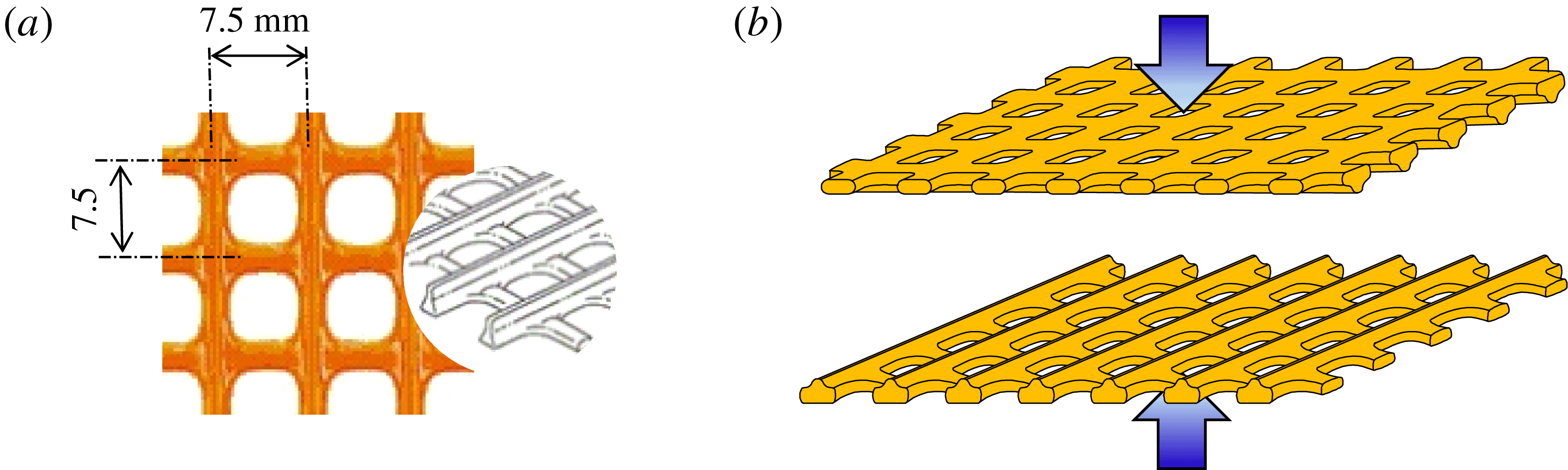
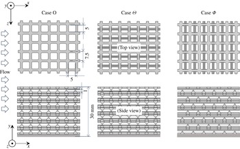
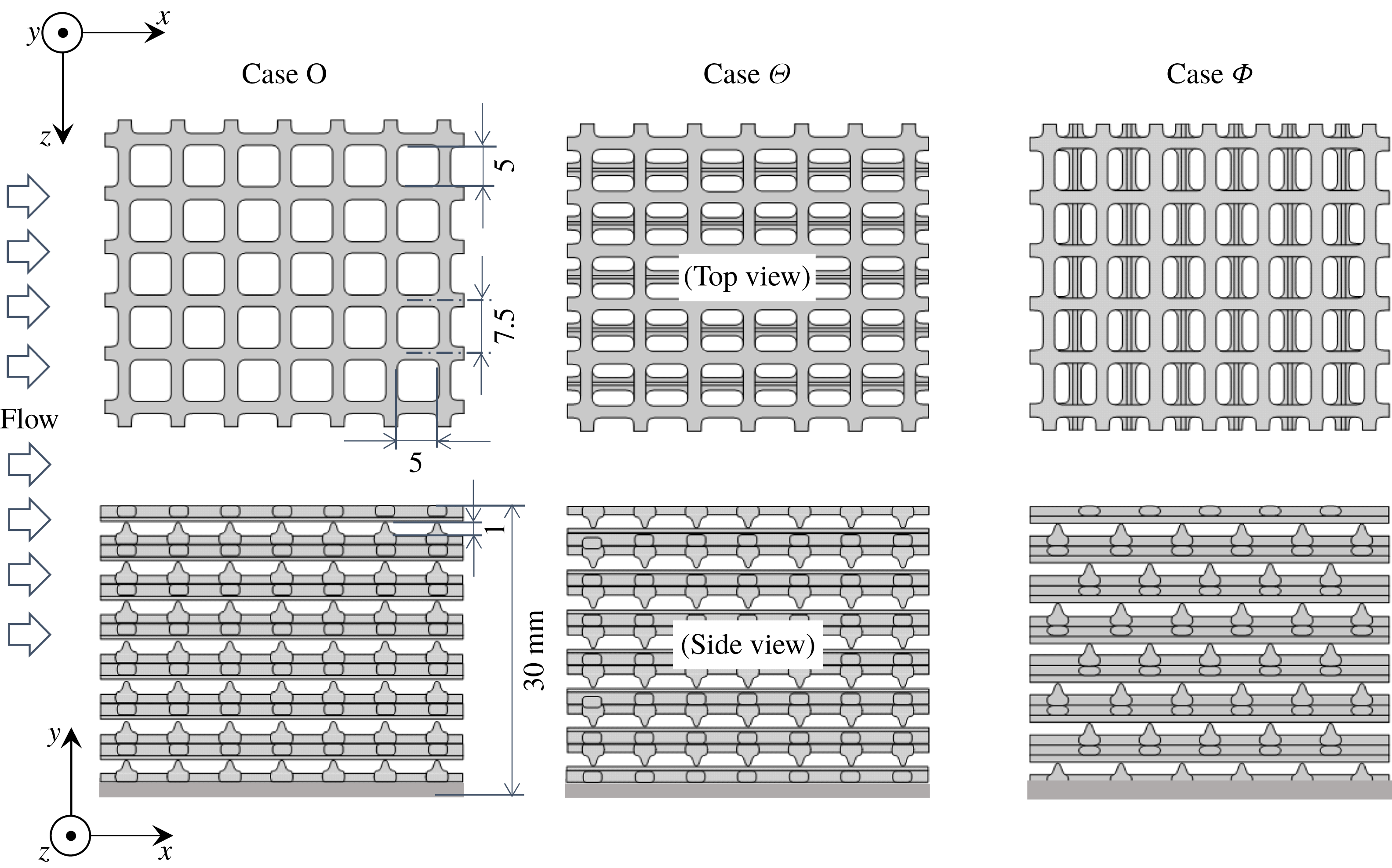
To construct the porous media, ethylene vinyl acetate (EVA) copolymer nets (N-523, Takiron) with rounded-square shaped pores, as shown in figure 1(a), are applied. Although one side of the net has a ribbed structure, the reverse side has a smooth surface. The porous media have layered structures of unit layers which are formed by bonding two nets, as shown in figure 1(b). Figure 2 shows three kinds of porous media made by different piling patterns of the layers in which the pore arrays are aligned with the Cartesian axes of the flow geometry. Since the specific gravity of EVA is 0.92–0.95, to increase the weight of the porous media lead plates are bonded to the very bottom layers. Porous medium case O is constructed by piling up the unit layers in a straight manner while case
 $\unicode[STIX]{x1D6E9}$
is made by an offset staggered piling up of the layers. Case
 $\unicode[STIX]{x1D6F7}$
is the same porous medium as case
 $\unicode[STIX]{x1D6E9}$
but its setting angle to the flow direction is turned
 $90^{\circ }$
. Note that cases O,
 $\unicode[STIX]{x1D6E9}$
and
 $\unicode[STIX]{x1D6F7}$
are named from the top views of the meshes. As seen in figure 2, all the structures have three mutually orthogonal principal axes and those principal axes are aligned with the Cartesian coordinate axes. In such cases, the porous media are called orthotropic porous media and their permeability tensors become diagonal (Dullien Reference Dullien1979). (This can be easily proved by manipulating Darcy’s law with macroscopic symmetry conditions.)
The characteristics of the porous media are measured as follows. For the porosity
 $\unicode[STIX]{x1D711}$
that is the ratio of the fluid phase volume
 $V_{f}$
and the total volume
 $V_{m}$
:
 $\unicode[STIX]{x1D711}=V_{f}/V_{m}$
, by measuring the perimeters of sample rectangular parallelepiped blocks,
 $V_{m}$
is obtained and its solid-phase volume
 $V_{s}$
is obtained by sinking the sample blocks into water contained in a measuring cylinder. Diagonal components of the permeability tensor
 $\unicode[STIX]{x1D612}_{\unicode[STIX]{x1D6FC}\unicode[STIX]{x1D6FC}}$
and the Forchheimer tensor
 $\unicode[STIX]{x1D60D}_{\unicode[STIX]{x1D6FC}\unicode[STIX]{x1D6FC}}$
are measured using a duct flow facility. In between the pressure holes, a porous block is placed to block the duct. Pressure drops
 $\unicode[STIX]{x2202}\langle p\rangle ^{f}/\unicode[STIX]{x2202}x_{\unicode[STIX]{x1D6FC}}$
along the
 $\unicode[STIX]{x1D6FC}$
-axis of the media and the flow rates are measured by a differential pressure gauge and a flow meter, respectively. With those variables at several different flow rates, the diagonal components of the permeability and Forchheimer tensors are obtained using the Darcy–Forchheimer equation of Whitaker (Reference Whitaker1986):
 $$\begin{eqnarray}\displaystyle \langle u_{i}\rangle =-\frac{\unicode[STIX]{x1D612}_{ij}}{\unicode[STIX]{x1D707}}\frac{\unicode[STIX]{x2202}\langle p\rangle ^{f}}{\unicode[STIX]{x2202}x_{j}}-\unicode[STIX]{x1D60D}_{ij}\langle u_{j}\rangle , & & \displaystyle\end{eqnarray}$$
Polymer net for constructing the porous media: (a) shape of the EVA copolymer net (N-523, Takiron), (b) forming a unit layer.

Three types of anisotropic porous media: cases O,
 $\unicode[STIX]{x1D6E9}$
and
 $\unicode[STIX]{x1D6F7}$
are named from the views of the meshes from the channel centre; lead plates are bonded to the very bottom layers to increase the weight.
where
 $\unicode[STIX]{x1D60D}_{ij}$
is the Forchheimer tensor currently modelled as
 $\unicode[STIX]{x1D60D}_{ij}=\unicode[STIX]{x1D70C}\unicode[STIX]{x1D60A}_{ij}^{F}|\langle \boldsymbol{u}\rangle |/\unicode[STIX]{x1D707}$
following the model by Nakayama et al. (Reference Nakayama, Kuwahara, Umemoto and Hayashi2002) while in their model, the Forchheimer coefficient tensor
 $\unicode[STIX]{x1D609}_{ij}^{F}$
was defined by
 $\unicode[STIX]{x1D60D}_{ij}=\unicode[STIX]{x1D70C}\unicode[STIX]{x1D612}_{ik}\unicode[STIX]{x1D609}_{kj}^{F}|\langle \boldsymbol{u}\rangle |/\unicode[STIX]{x1D707}$
. (In this case, the Forchheimer tensor explicitly depends on the permeability tensor.) The Darcy velocity
 $\langle u_{i}\rangle$
is obtained from the measured flow rate. Note that for a material whose structure is symmetric in the
 $x$
-,
 $y$
- and
 $z$
-directions, the Forchheimer tensor becomes diagonal. (This can be proved by manipulating equation (2.1) with the symmetry conditions.) As seen in figure 2, the structures of the present porous media are symmetric in the
 $x$
- and
 $z$
-directions while they are not strictly symmetric in the
 $y$
-direction. The side views of the pore shapes are asymmetric in the
 $y$
-direction, though they are not very far from symmetric. Hence, we assume that the effects of the off-diagonal components of the Forchheimer tensor on the measurement of the characteristics of the porous media are insignificant. The measured variables of the present porous media are listed in table 1. Although the porosity is constant for all three cases as
 $\unicode[STIX]{x1D711}=0.7$
, to study the effects of the anisotropic permeability on turbulence, the wall-normal diagonal component of the permeability tensor
 $\unicode[STIX]{x1D612}_{yy}$
is designed to be larger than the other components by factors of 1.2, 1.5 and 173. As for the Forchheimer tensor, the coefficient
 $\unicode[STIX]{x1D60A}_{ij}^{F}$
is nearly isotropic in cases
 $\unicode[STIX]{x1D6E9}$
and
 $\unicode[STIX]{x1D6F7}$
while it is anisotropic in case O with larger
 $\unicode[STIX]{x1D60A}_{yy}^{F}$
than the other components by a factor of 76.
Characteristics of the anisotropic porous media:
 $\unicode[STIX]{x1D711}$
is the porosity;
 $\unicode[STIX]{x1D612}_{xx}$
,
 $\unicode[STIX]{x1D612}_{yy}$
and
 $\unicode[STIX]{x1D612}_{zz}$
are the diagonal components of the permeability tensor;
 $\unicode[STIX]{x1D60A}_{xx}^{F}$
,
 $\unicode[STIX]{x1D60A}_{yy}^{F}$
and
 $\unicode[STIX]{x1D60A}_{zz}^{F}$
are the diagonal components of the coefficient of the Forchheimer tensor.

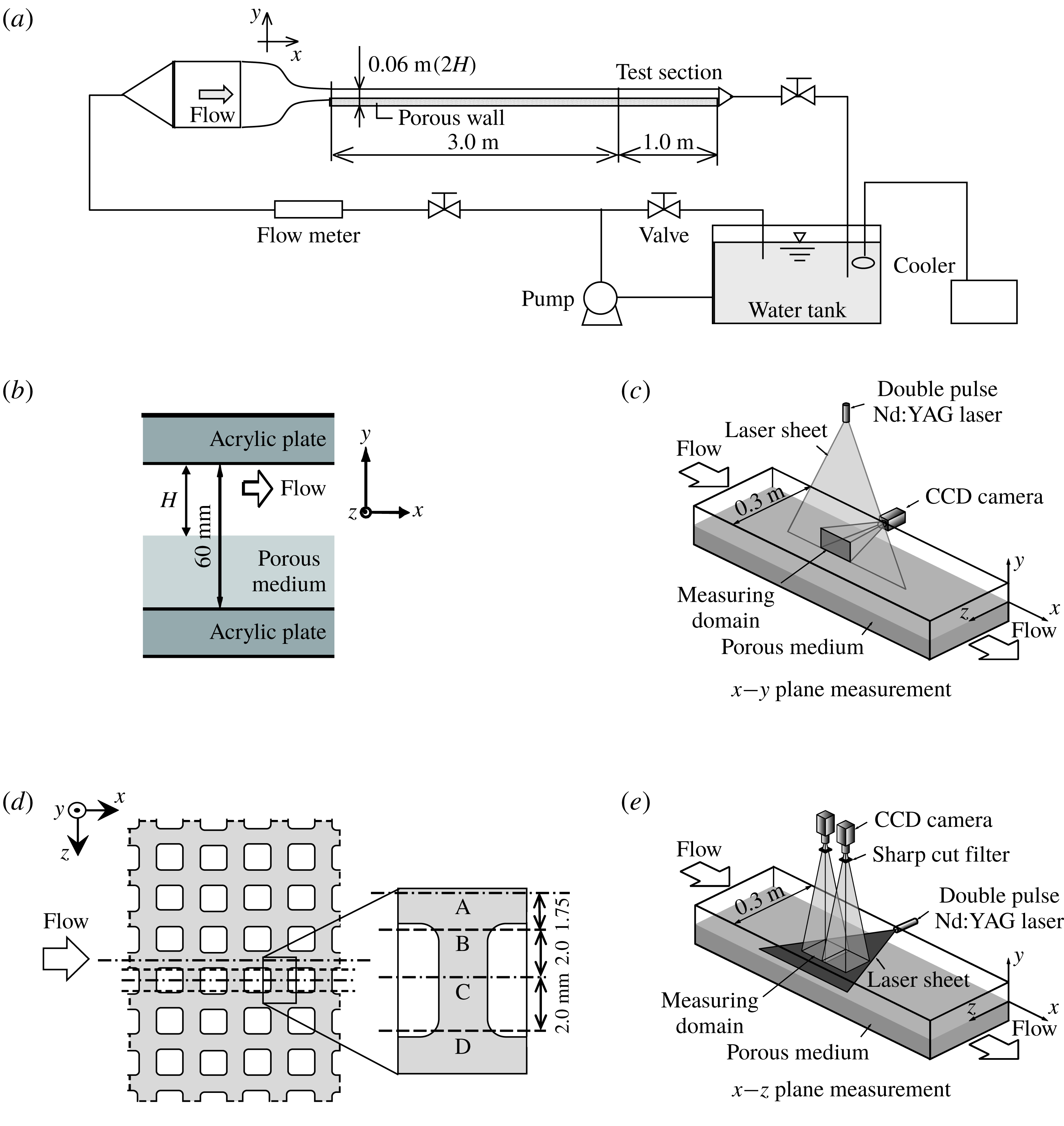
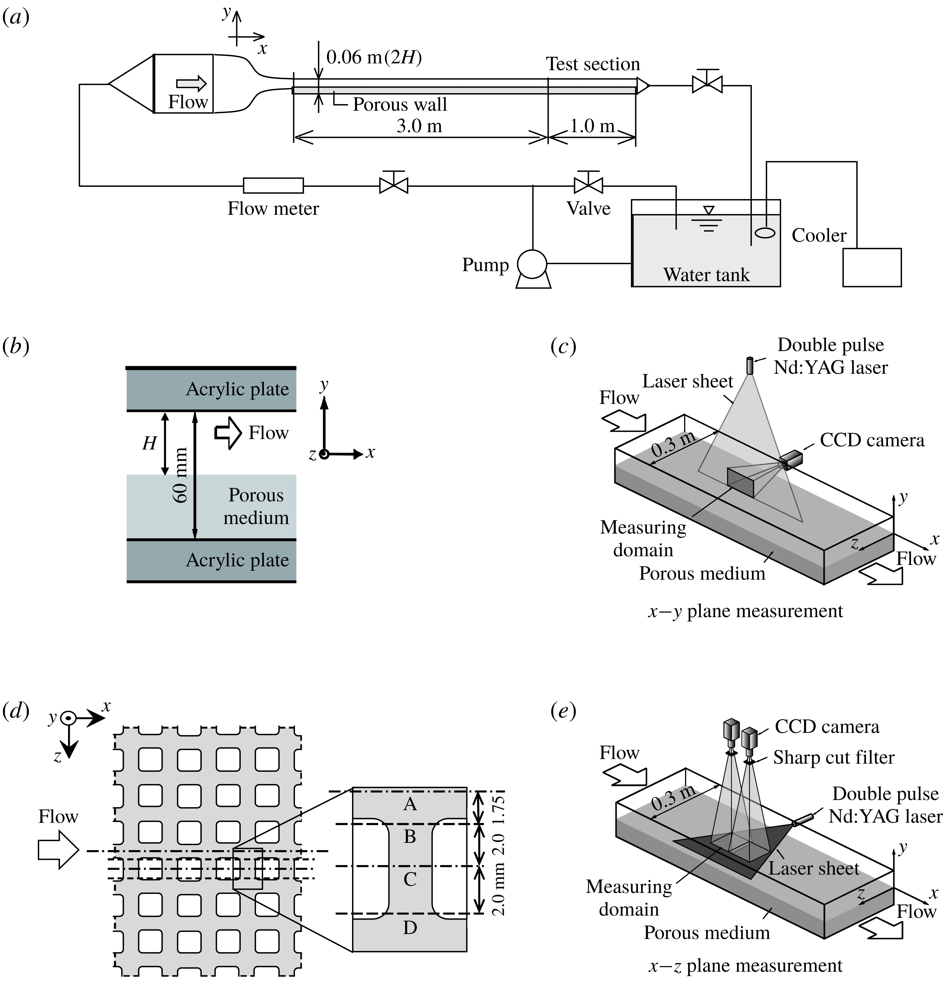
Figure 3(a) illustrates the experimental flow facility. Tap water, whose temperature is maintained by a cooler at
 $285\pm 1~\text{K}$
, is pumped to a digital flow meter (FD-MH200A/500A, KEYENCE) where its total flow rate is measured. The water temperature is recorded by a digital thermometer (FD-T1, KEYENCE) in a honeycomb-bundled nozzle. After the flow is conditioned by the honeycomb-bundled nozzle and fully developed in a driver section whose length is 3.0 m, it enters the test section whose length is 1.0 m. As illustrated in figure 3(b), both sections consist of solid smooth acrylic walls with a porous bottom layer. The sectional width
 $W$
and the total height are, respectively, 0.3 m and 0.06 m which is filled by a 0.03 m thick porous layer. Since the height of the clear fluid region is set to
 $H=0.03~\text{m}$
, the aspect ratio of the cross-section of the clear fluid region is approximately 10. Accordingly, two-dimensionality can be reasonably attained in
 $z/W=0.1{-}0.9$
which was confirmed and reported by the previous study (Suga et al.
Reference Suga, Nakagawa and Kaneda2017). The measured range of the bulk Reynolds number
 $Re_{b}$
(
 $\unicode[STIX]{x1D70C}U_{b}H/\unicode[STIX]{x1D707}$
) is 900–13 600 where the fluid viscosity
 $\unicode[STIX]{x1D707}$
and density
 $\unicode[STIX]{x1D70C}$
are determined by the measured water temperature. Here, the bulk mean velocity
 $U_{b}$
is obtained by integrating the measured cross-sectional streamwise mean velocity distribution while the wall shear stress is estimated by extrapolating the Reynolds shear stress distribution obtained by the
 $x$
–
 $y$
plane measurement.
Experimental set-up: (a) flow facility, (b) cross-sectional view of the test section, (c) schematic view of the streamwise–wall-normal (
 $x$
–
 $y$
) plane measurements, (d) locations of the measured planes A, B, C and D for volume averaging the
 $x$
–
 $y$
plane measurements, (e) schematic view of the streamwise–spanwise (
 $x$
–
 $z$
) plane measurements.
The applied planar PIV system consists of a double-pulse Nd:YAG laser (Dual Power 200-15, Litron) with
 $200~\text{mJ}~\text{pulse}^{-1}$
at a wavelength of 532 nm. For the measurements of the streamwise–wall-normal (
 $x$
–
 $y$
) planes, the laser beam is formed into a sheet of approximately 1.0 mm thickness through several cylindrical lenses and illuminates the measuring planes as shown in figure 3(c). The recorded frame of a CCD camera (FlowSense 4M Mk2, Dantec Dynamics) operating at 30 frames per second with 85 mm
 $f/1:8$
lenses (AF Nikkor, Nikon) covers a section of
 $30(x)\times 30(y)~\text{mm}^{2}$
located in the middle part of the test section with
 $2048\times 2048$
pixels. This frame covers four pore cells of the porous media in the
 $x$
-direction. To obtain the
 $x$
–
 $z$
plane-averaged time mean quantities in the
 $y$
-direction, the flow fields are measured at four
 $x$
–
 $y$
sections, A, B, C and D, from the symmetry plane of the channel, as shown in figure 3(d). Using time mean field data, streamwise averaging is carried out for each section. Then, with the streamwise-averaged data of the four sections, integration by the trapezoidal rule is applied to the spanwise averaging. It has been confirmed that the four plane measurements are good enough for the spanwise averaging by comparing the results with those obtained by the measurement of six planes which divide the unit pore cell equally (1.25 mm pitch). Note that the integration by six plane measurement data is nearly ideal for the volume averaging since the pore pitch and the approximate laser sheet thickness are 7.5 mm and 1 mm, respectively. Accordingly, the present plane-averaged values are from the plane of
 $4(x)\times 1(z)$
pore cells of the porous media. For the measurements of the streamwise–spanwise (
 $x$
–
 $z$
) planes, the laser sheet of approximately 1.0 mm thickness illuminates the
 $x$
–
 $z$
planes as shown in figure 3(e). Two CCD cameras are arranged in tandem. The recorded frame of each CCD camera covers a zone of
 $81\times 81~\text{mm}^{2}$
located in the middle of the test section with 2048
 $\times$
2048 pixels, for which 10 % of the area overlaps with another camera’s frame. The measured planes are located at
 $y=1.0$
, 2.0, 3.0, 4.0, 5.0 mm while additional planes are occasionally measured. Note that the origin of the
 $y$
-axis is set at the porous surface.
For the tracer particles of the
 $x$
–
 $y$
plane measurements, acrylic colloid particles are used. The mean diameter, specific gravity and refractive index of the particles are respectively
 $3.1~\unicode[STIX]{x03BC}\text{m}$
, 1.19 and 1.50. For the
 $x$
–
 $z$
plane measurements, to avoid the noisy Mie scattering from the wall surface, polymer fluorescent particles containing Rhodamine B, whose mean diameter and specific gravity are respectively
 $10~\unicode[STIX]{x03BC}\text{m}$
and 1.50, are used. Correspondingly, a long-pass filter with cutoff wavelength 560 nm is located in front of each camera lens. In both cases, the seeding density is adjusted to obtain 10–15 particle image pairs in each interrogation window whose size is set to 32
 $\times$
32 pixels. Thus the measurement sampling volumes are
 $0.4(x)\times 0.4(y)\times 1.0(z)~\text{mm}^{3}$
and
 $0.4(x)\times 1.0(y)\times 0.4(z)~\text{mm}^{3}$
, respectively for the
 $x$
–
 $y$
and
 $x$
–
 $z$
measurements. The image sampling rate was 4 Hz. The average particle displacement was set to be approximately 25 % of the length (6–8 pixels) of the interrogation window. To obtain the statistical data, more than 4000 image pairs are processed. The recorded data are processed by the Dynamics Studio 3.1 software (Dantec Dynamics) with the fast Fourier transform cross-correlation technique (Willert & Gharib Reference Willert and Gharib1991). Each image is processed to produce 127
 $\times$
127 vectors from the interrogation windows with 50 % overlap in each direction. When the ratio of the first and the second correlation peaks in an interrogation window is smaller than 1.3, the corresponding vector is removed from the process as an error vector. Furthermore, the moving-average validation (Host-Madsen & McCluskey Reference Host-Madsen and McCluskey1994) is applied with an acceptance factor of 0.1. In the present study, the removed error vectors are less than 3 % of the total data processed.
Following Prasad et al. (Reference Prasad, Adrian, Landreth and Offutt1992), it is confirmed that the particle images are well resolved in the present experiments, and the uncertainty in the measured displacement can be expected to be approximately less than
 $1/10$
th of the diameter of the particle image. Normalizing this uncertainty by the mean displacement length of the particles indicates that the estimated error in the magnitude of the instantaneous velocity is less than 4 % of the maximum velocity near the channel centreline.
3 Results and discussions
3.1 Streamwise–wall-normal plane measurements
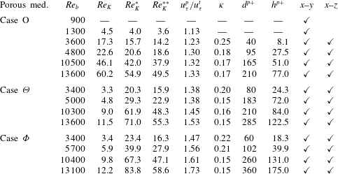
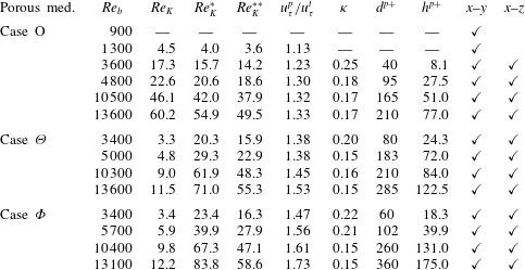
Table 2 lists the experimental conditions and measured parameters which are discussed below. For case O, the measured flows are at
 $Re_{b}=900$
, 1300, 3600, 4800, 10 500 and 13 600, while for cases
 $\unicode[STIX]{x1D6E9}$
and
 $\unicode[STIX]{x1D6F7}$
they are at
 $Re_{b}=3400$
, 5000, 10 300, 13 600 and
 $Re_{b}=3400$
, 5700, 10 400, 13 600, respectively. In the following discussion, the
 $x$
–
 $z$
plane-averaged value of
 $\unicode[STIX]{x1D719}$
is denoted as
 $[\unicode[STIX]{x1D719}]$
and the Reynolds-averaged
 $\unicode[STIX]{x1D719}$
is denoted as
 $\bar{\unicode[STIX]{x1D719}}$
with the Reynolds decomposition
 $\unicode[STIX]{x1D719}=\bar{\unicode[STIX]{x1D719}}+\unicode[STIX]{x1D719}^{\prime }$
. For simplicity, the plane- and Reynolds-averaged velocity is called the ‘mean velocity’ hereafter.
Experimental conditions and measured parameters of the mean velocity fields:
 $Re_{b}$
,
 $Re_{K}$
,
 $Re_{K}^{\ast }$
and
 $Re_{K}^{\ast \ast }$
are the bulk Reynolds number, the permeability Reynolds number defined by (3.3), the generalized permeability Reynolds number defined by (3.10) and the surrogate permeability Reynolds number defined by (3.11);
 $u_{\unicode[STIX]{x1D70F}}^{t}$
and
 $u_{\unicode[STIX]{x1D70F}}^{p}$
are the friction velocities on the top solid and bottom porous walls;
 $\unicode[STIX]{x1D705},d$
and
 $h$
are the von Kármán coefficient, the zero-plane displacement and the roughness scale, respectively;
 $(\cdot )^{p+}$
corresponds to a value normalized by using
 $u_{\unicode[STIX]{x1D70F}}^{p}$
.
3.1.1 Mean velocity
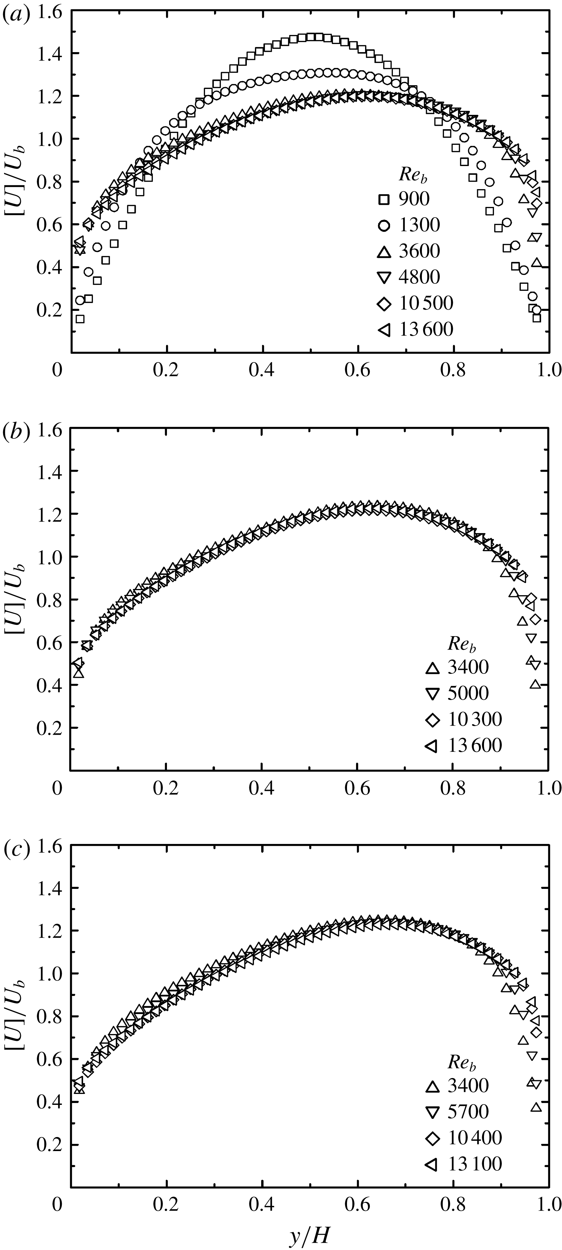
Figure 4 shows the streamwise mean velocity
 $[U]\,(=[\bar{u}_{x}])$
profiles. In case O, as seen in figure 4(a) at
 $Re_{b}=900$
, the velocity profile is parabolic, implying that the flow is laminar, but from
 $Re_{b}=1300$
the profile becomes asymmetric, indicating that the laminar to turbulent transition occurs in this range of the Reynolds number. Once the flow becomes fully turbulent at
 $Re_{b}\geqslant 3600$
, there is no significant change in the profiles. This tendency and the general slanted profiles to the porous walls are maintained in cases
 $\unicode[STIX]{x1D6E9}$
and
 $\unicode[STIX]{x1D6F7}$
as seen in figure 4(b,c). The slippage velocities on the porous surfaces are approximately
 $[U_{w}]/U_{b}=0.4$
at
 $Re_{b}\geqslant 3600$
which are similar to those over the isotropic porous media reported in the previous study (Suga et al.
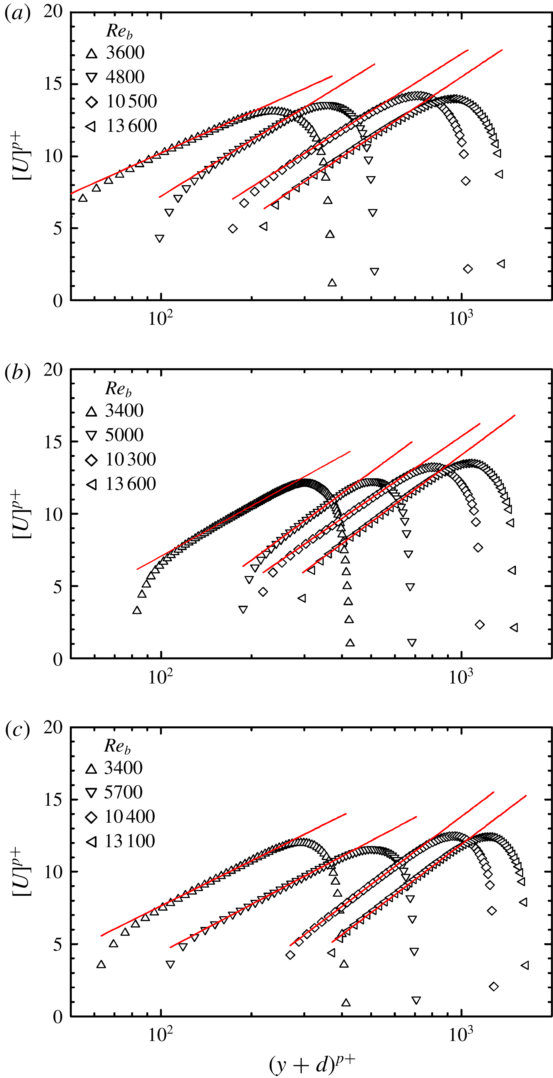
Reference Suga, Matsumura, Ashitaka, Tominaga and Kaneda2010). These velocity profiles are replotted in semi-logarithmic charts as shown in figure 5. The fitted lines are of the log-law form that is usually applied to the flows over porous media and canopies (Best Reference Best1935; Nikora et al.
Reference Nikora, Koll, McLean, Dittrich and Aberle2002; Nepf & Ghisalberti Reference Nepf and Ghisalberti2008). That is,
 $$\begin{eqnarray}\displaystyle [U]^{p+}=\frac{1}{\unicode[STIX]{x1D705}}\ln \left(\frac{y+d}{h}\right), & & \displaystyle\end{eqnarray}$$
with the von Kármán constant
 $\unicode[STIX]{x1D705}$
, the zero-plane displacement
 $d$
and the roughness scale
 $h$
. Here,
 $[U]^{p+}=[U]/u_{\unicode[STIX]{x1D70F}}^{p}$
and the friction velocity
 $u_{\unicode[STIX]{x1D70F}}^{p}$
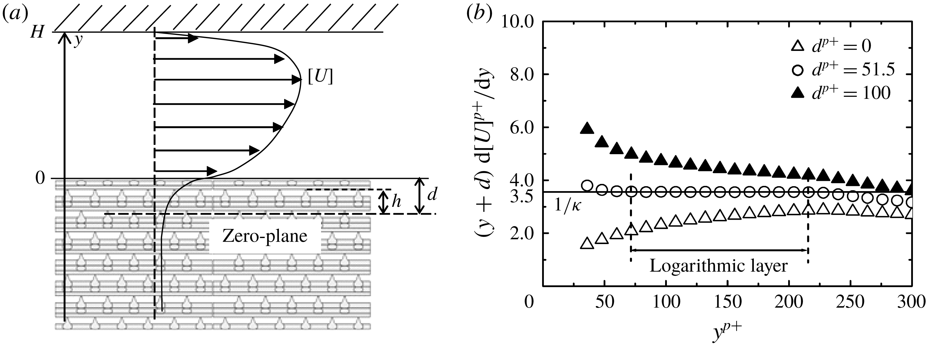
on the porous wall is estimated by extrapolating the plane-averaged Reynolds shear stress distribution measured by this study. Figure 6(a) shows illustrative definitions of
 $d$
and
 $h$
. They are the displacement of the origin of the
 $y$
-axis and the equivalent roughness height from the zero plane, respectively. Table 2 lists the values of
 $\unicode[STIX]{x1D705}$
,
 $d^{p+}(=u_{\unicode[STIX]{x1D70F}}^{p}d/\unicode[STIX]{x1D708})$
and
 $h^{p+}(=u_{\unicode[STIX]{x1D70F}}^{p}h/\unicode[STIX]{x1D708})$
which are obtained as follows. The extent of the logarithmic layer can be determined from plots of
 $(y+d)\,\text{d}[U]^{p+}/\text{d}y$
as a function of
 $y^{p+}(=yu_{\unicode[STIX]{x1D70F}}^{p}/\unicode[STIX]{x1D708})$
changing the values of
 $d$
(Breugem et al.
Reference Breugem, Boersma and Uittenbogaard2006). Since
 $(y+d)\,\text{d}[U]^{p+}/\text{d}y$
must be a constant equal to
 $1/\unicode[STIX]{x1D705}$
inside the logarithmic layer, a value of
 $d$
giving a flat plateau in the profile must be the best fitted value. For example, in figure 6(b), a flat plateau can be obtained with
 $d^{p+}=51.5$
and the value of the plateau becomes
 $(y+d)\,\text{d}[U]^{p+}/\text{d}y=3.5$
which corresponds to
 $1/\unicode[STIX]{x1D705}$
to be obtained. Then, with these
 $d$
and
 $\unicode[STIX]{x1D705}$
, equation (3.1) is best fitted to the velocity profile to obtain the roughness length scale
 $h$
.
Mean velocity distributions: (a) case O, (b) case
 $\unicode[STIX]{x1D6E9}$
, (c) case
 $\unicode[STIX]{x1D6F7}$
.

Mean velocity distributions in semi-log scale: (a) case O, (b) case
 $\unicode[STIX]{x1D6E9}$
, (c) case
 $\unicode[STIX]{x1D6F7}$
; lines are fitting lines.

Parameters of mean velocity: (a) zero-plane displacement
 $d$
and roughness length scale
 $h$
, (b) logarithmic layer indicated by
 $(y+d)\,\text{d}[U]^{p+}/\text{d}y$
.

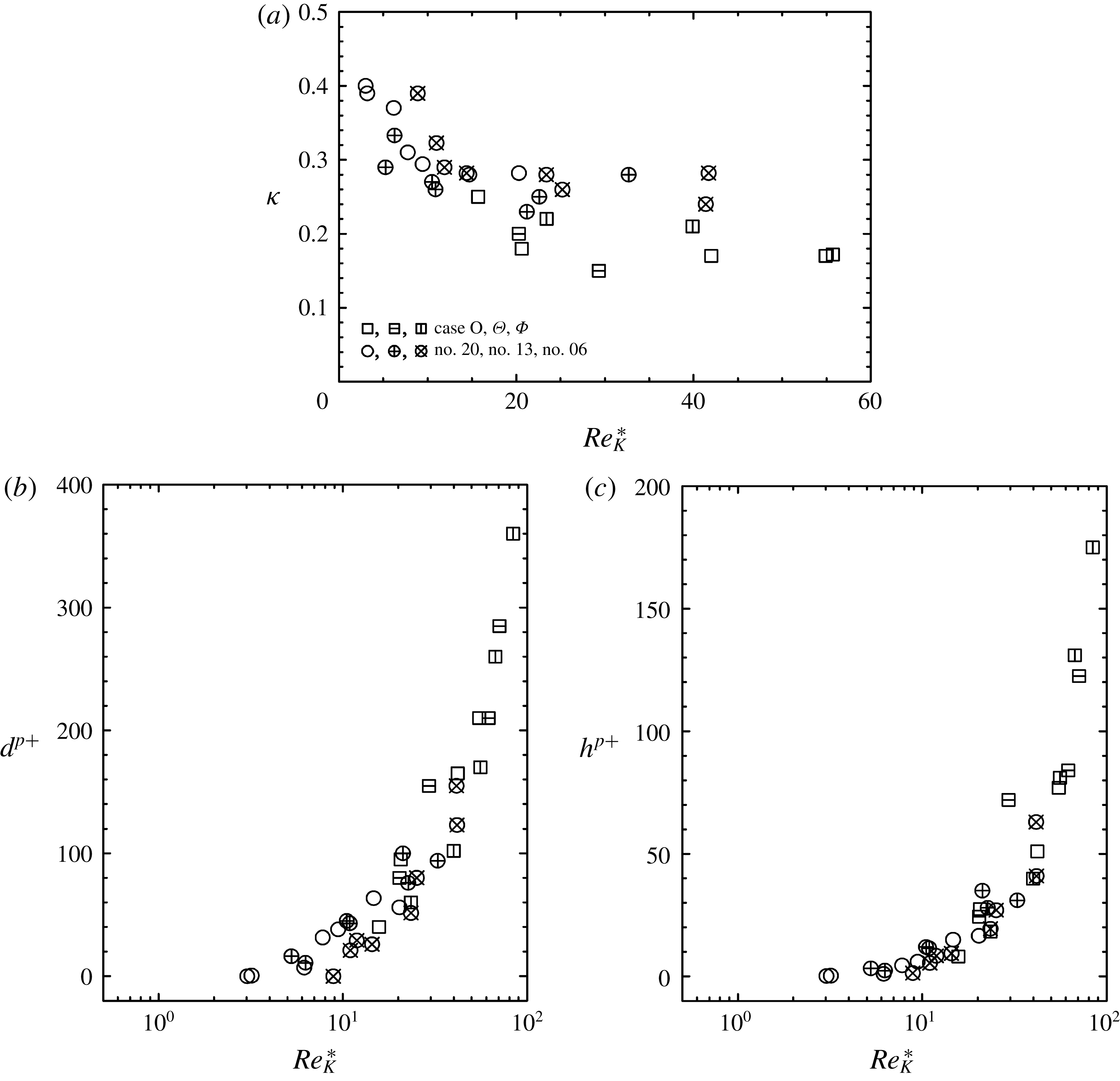
Distributions of log-law parameters against the permeability Reynolds number
 $Re_{K}$
: (a) zero-plane displacement, and (b) roughness scale; no. 20, no. 13 and no. 06 are the isotropic cases at
 $\unicode[STIX]{x1D711}=0.8$
of Suga et al. (Reference Suga, Matsumura, Ashitaka, Tominaga and Kaneda2010, Reference Suga, Nakagawa and Kaneda2017).

It is obvious that the slope of the fitted line, and hence
 $\unicode[STIX]{x1D705}$
, varies with
 $Re_{b}$
. This trend is the same as that reported in the previous studies (Suga et al.
Reference Suga, Matsumura, Ashitaka, Tominaga and Kaneda2010, Reference Suga, Nakagawa and Kaneda2017) in which obvious correlations between the permeability Reynolds number
 $Re_{K}$
and the parameters
 $\unicode[STIX]{x1D705}$
,
 $d$
and
 $h$
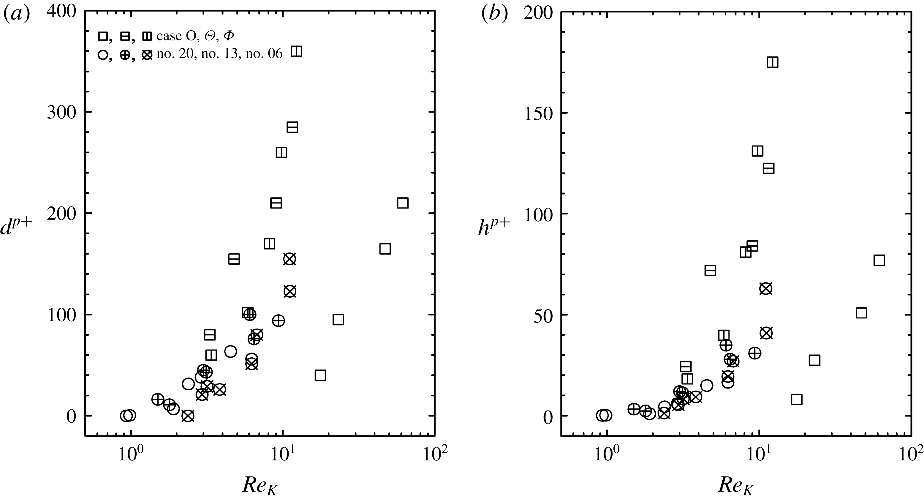
were reported. However, as shown in figure 7, it is seen that such correlations with
 $Re_{K}$
cannot be seen in the present data, particularly for
 $d$
and
 $h$
. For the anisotropic porous media,
 $K$
is currently defined as
 $$\begin{eqnarray}\displaystyle K=\unicode[STIX]{x1D612}_{kk}/3=(\unicode[STIX]{x1D612}_{xx}+\unicode[STIX]{x1D612}_{yy}+\unicode[STIX]{x1D612}_{zz})/3, & & \displaystyle\end{eqnarray}$$
which corresponds to
 $1/3$
of the trace of the permeability tensor and this maintains consistency with the isotropic permeability. Hence, in this study the permeability Reynolds number is defined as
 $$\begin{eqnarray}\displaystyle Re_{K}=\frac{u_{\unicode[STIX]{x1D70F}}^{p}\sqrt{\unicode[STIX]{x1D646}_{kk}/3}}{\unicode[STIX]{x1D708}}. & & \displaystyle\end{eqnarray}$$
Table 2 lists
 $Re_{K}$
for each case. Since the values of
 $Re_{K}$
in case O are significantly larger than those in cases
 $\unicode[STIX]{x1D6E9}$
and
 $\unicode[STIX]{x1D6F7}$
, the plots of case O in figure 7 significantly deviate from the other plots. Also, another form,
 $K=(\unicode[STIX]{x1D612}_{xx}\unicode[STIX]{x1D612}_{yy}\unicode[STIX]{x1D612}_{zz})^{1/3}$
, whose concept is from Chan, Larive & Morgan (Reference Chan, Larive and Morgan1993), leads to much larger values of
 $Re_{K}$
in case O and produces more unsuccessful results than those shown in figure 7. These results suggest that anisotropic effects of the permeability and/or the Forchheimer tensor play important roles in determining the flow characteristics.
3.1.2 Generalization of the characteristic Reynolds number
Since the zero-plane displacement
 $d$
and the roughness scale
 $h$
are defined as the values inside porous surfaces, we discuss the transport equations inside the porous media. In the double (Reynolds and volume) averaging process, Pedras & de Lemos (Reference Pedras and de Lemos2000) proved that the order of the averaging operations is interchangeable. When the following decomposition for the volume averaging,
 $\unicode[STIX]{x1D719}=\langle \unicode[STIX]{x1D719}\rangle +\tilde{\unicode[STIX]{x1D719}}$
, is applied, the interchangeable operations lead to
 $\overline{\langle \unicode[STIX]{x1D719}\rangle }=\langle \bar{\unicode[STIX]{x1D719}}\rangle$
,
 $\langle \unicode[STIX]{x1D719}\rangle ^{\prime }=\langle \unicode[STIX]{x1D719}^{\prime }\rangle$
,
 $\tilde{\unicode[STIX]{x1D719}^{\prime }}=(\tilde{\unicode[STIX]{x1D719}})^{\prime }$
and
 $\tilde{\bar{\unicode[STIX]{x1D719}}}=\bar{\tilde{\unicode[STIX]{x1D719}}}$
. Then, the double-averaged continuity and momentum equations in porous media may be written as
 $$\begin{eqnarray}\displaystyle & \displaystyle \frac{\unicode[STIX]{x2202}\unicode[STIX]{x1D711}\langle \bar{u}_{i}\rangle ^{f}}{\unicode[STIX]{x2202}x_{i}}=0, & \displaystyle\end{eqnarray}$$
 $$\begin{eqnarray}\displaystyle & \displaystyle \frac{\unicode[STIX]{x2202}\langle \bar{u}_{i}\rangle ^{f}}{\unicode[STIX]{x2202}t}+\langle \bar{u}_{j}\rangle ^{f}\frac{\unicode[STIX]{x2202}\langle \bar{u}_{i}\rangle ^{f}}{\unicode[STIX]{x2202}x_{j}}=-\frac{1}{\unicode[STIX]{x1D70C}}\frac{\unicode[STIX]{x2202}\langle \bar{p}\rangle ^{f}}{\unicode[STIX]{x2202}x_{i}}+\unicode[STIX]{x1D708}\frac{\unicode[STIX]{x2202}^{2}\langle \bar{u}_{i}\rangle ^{f}}{\unicode[STIX]{x2202}x_{j}^{2}}-\frac{1}{\unicode[STIX]{x1D711}}\frac{\unicode[STIX]{x2202}}{\unicode[STIX]{x2202}x_{j}}(\unicode[STIX]{x1D711}\langle \unicode[STIX]{x1D619}_{ij}\rangle ^{f})-\frac{1}{\unicode[STIX]{x1D711}}\frac{\unicode[STIX]{x2202}}{\unicode[STIX]{x2202}x_{j}}(\unicode[STIX]{x1D711}\langle \unicode[STIX]{x1D61B}_{ij}\rangle ^{f})-\bar{f}_{i}, & \displaystyle \nonumber\\ \displaystyle & & \displaystyle\end{eqnarray}$$
where the symbolic notations of the volume-averaged Reynolds stress and the dispersion stress (or dispersive covariance: see Raupach & Shaw (Reference Raupach and Shaw1982)) are
 $\langle \unicode[STIX]{x1D619}_{ij}\rangle ^{f}=\langle \overline{u_{i}^{\prime }u_{j}^{\prime }}\rangle ^{f}$
and
 $\langle \unicode[STIX]{x1D61B}_{ij}\rangle ^{f}=\langle \bar{\tilde{u} }_{i}\bar{\tilde{u} }_{j}\rangle ^{f}$
, respectively. Note that for the volume averaging, there is a relation
 $\unicode[STIX]{x1D711}\langle \unicode[STIX]{x1D719}\rangle ^{f}=\langle \unicode[STIX]{x1D719}\rangle$
. With the link to equation (2.1), the drag force term
 $f_{i}$
derived by Whitaker (Reference Whitaker1996) is
 $$\begin{eqnarray}\displaystyle f_{i}=\underbrace{\unicode[STIX]{x1D711}\unicode[STIX]{x1D708}\unicode[STIX]{x1D612}_{ij}^{-1}\langle u_{j}\rangle ^{f}}_{\text{viscous}\;\text{drag}}+\underbrace{\unicode[STIX]{x1D711}\unicode[STIX]{x1D708}\unicode[STIX]{x1D612}_{ik}^{-1}\unicode[STIX]{x1D60D}_{kj}\langle u_{j}\rangle ^{f}}_{\text{form}\;\text{drag}}. & & \displaystyle\end{eqnarray}$$
Accordingly, when
 $\unicode[STIX]{x1D612}_{ij}$
is diagonal and the Forchheimer tensor is modelled as
 $\unicode[STIX]{x1D60D}_{ij}=\unicode[STIX]{x1D70C}\unicode[STIX]{x1D60A}_{ij}^{F}|\langle \boldsymbol{u}\rangle |/\unicode[STIX]{x1D707}$
, the force terms for the double-averaged fields of fully developed flows (the streamwise and wall-normal directions are aligned with the
 $x$
- and
 $y$
-axes, respectively) are
 $$\begin{eqnarray}\displaystyle & \displaystyle \bar{f}_{x}=\unicode[STIX]{x1D708}\unicode[STIX]{x1D612}_{xx}^{-1}\langle \bar{u}_{x}\rangle +\unicode[STIX]{x1D612}_{xx}^{-1}\{\unicode[STIX]{x1D60A}_{xx}^{F}(\overline{|\langle \boldsymbol{u}\rangle |}\langle \bar{u}_{x}\rangle +\overline{|\langle \boldsymbol{u}\rangle |^{\prime }\langle u_{x}^{\prime }\rangle })+\unicode[STIX]{x1D60A}_{xy}^{F}(\overline{|\langle \boldsymbol{u}\rangle |^{\prime }\langle u_{y}^{\prime }\rangle })\}, & \displaystyle\end{eqnarray}$$
 $$\begin{eqnarray}\displaystyle & \displaystyle \bar{f}_{y}=\unicode[STIX]{x1D612}_{yy}^{-1}\{C_{yx}^{F}(\overline{|\langle \boldsymbol{u}\rangle |^{\prime }\langle u_{x}^{\prime }\rangle })+\unicode[STIX]{x1D60A}_{yy}^{F}(\overline{|\langle \boldsymbol{u}\rangle |^{\prime }\langle u_{y}^{\prime }\rangle })\}, & \displaystyle\end{eqnarray}$$
since
 $\langle \bar{u}_{y}\rangle =\langle \bar{u}_{z}\rangle =0$
. The above equation (3.7) indicates that the streamwise permeability
 $\unicode[STIX]{x1D612}_{xx}$
directly affects the streamwise mean velocity inside porous media with the
 $x$
–
 $x$
and
 $x$
–
 $y$
components of
 $\unicode[STIX]{x1D60A}_{ij}^{F}$
. Furthermore, as shown in (3.5), since the double-averaged momentum equation includes the contribution from the volume-averaged Reynolds stress
 $\langle \unicode[STIX]{x1D619}_{ij}\rangle ^{f}$
and the dispersion stress
 $\langle \unicode[STIX]{x1D61B}_{ij}\rangle ^{f}$
, the budget terms of the shear stresses
 $\langle \unicode[STIX]{x1D619}_{xy}\rangle ^{f}$
and
 $\langle \unicode[STIX]{x1D61B}_{xy}\rangle ^{f}$
should be considered for the streamwise velocity. (See appendix A for the stress transport equations.) Among them there is no drag force related term in the
 $\langle \unicode[STIX]{x1D619}_{ij}\rangle ^{f}$
transport equation (A 1) as derived by Pinson, Grégoire & Simonin (Reference Pinson, Grégoire and Simonin2006), Nezu & Sanjou (Reference Nezu and Sanjou2008) and Kuwata & Suga (Reference Kuwata and Suga2015), but the drag work term
 $\bar{f_{i}}\langle \bar{u}_{j}\rangle +\bar{f_{j}}\langle \bar{u}_{i}\rangle$
appears in the
 $\langle \unicode[STIX]{x1D61B}_{ij}\rangle ^{f}$
transport equation (A 2) as shown in Pinson et al. (Reference Pinson, Grégoire and Simonin2006) and Kuwata, Suga & Sakurai (Reference Kuwata, Suga and Sakurai2014). Hence,
 $\bar{f_{y}}\langle \bar{u}_{x}\rangle$
affects the mean velocity profile indirectly via
 $\langle \unicode[STIX]{x1D61B}_{xy}\rangle ^{f}$
. Accordingly, coupling with the Forchheimer terms,
 $\unicode[STIX]{x1D612}_{yy}$
influences the streamwise velocity as the Reynolds number increases. However, it is expected that the primary effect on the mean flow profile comes from the streamwise permeability
 $\unicode[STIX]{x1D612}_{xx}$
via
 $\bar{f}_{x}$
when the Reynolds number is not significantly high. (Note that this is for the diagonal
 $\unicode[STIX]{x1D612}_{ij}$
cases and not for the general anisotropic cases.) Furthermore, considering the fact that meaningful classification of turbulent flows by the permeability Reynolds number was reported by Breugem et al. (Reference Breugem, Boersma and Uittenbogaard2006) at
 $Re_{b}=5500$
and by Manes et al. (Reference Manes, Poggi and Ridol2011) at
 $Re_{b}<10^{5}$
, the following discussion focuses on modifying the permeability Reynolds number using the streamwise permeability.
Although simply replacing
 $K$
with
 $\unicode[STIX]{x1D612}_{xx}$
for
 $Re_{K}$
may improve the correlation, to include the effects of the porosity in the characterization, we consider the Kozeny–Carman equation (Kozeny Reference Kozeny1927; Carman Reference Carman1937, Reference Carman1956):
 $$\begin{eqnarray}\displaystyle \frac{\text{d}\langle p\rangle ^{f}}{\text{d}x}=-\frac{150\unicode[STIX]{x1D707}}{d_{g}^{2}\unicode[STIX]{x1D6F7}_{s}^{2}}\frac{(1-\unicode[STIX]{x1D711})^{2}}{\unicode[STIX]{x1D711}^{3}}\langle u_{x}\rangle , & & \displaystyle\end{eqnarray}$$
where
 $\unicode[STIX]{x1D6F7}_{s}$
is the sphericity of the particles in the packed bed and
 $d_{g}$
is the diameter of the related spherical particle. Combining equation (3.9) with the Darcy equation (1.1) yields the relationship between
 $d_{g}$
and permeability as
 $\sqrt{(180(1-\unicode[STIX]{x1D711})^{2}/\unicode[STIX]{x1D711}^{3})\unicode[STIX]{x1D612}_{xx}}=d_{g}$
, where
 $150/\unicode[STIX]{x1D6F7}_{s}^{2}$
is replaced by 180 following Macdonald et al. (Reference Macdonald, El-Sayed, Mow and Dullen1979). When
 $\unicode[STIX]{x1D612}_{xx}$
is measurable, the newly defined length scale
 $d_{K_{x}}=\sqrt{(180(1-\unicode[STIX]{x1D711})^{2}/\unicode[STIX]{x1D711}^{3})\unicode[STIX]{x1D612}_{xx}}$
may be regarded as a characteristic streamwise length scale for the porous medium rather than the particle diameter. Using
 $d_{K_{x}}$
, a characteristic Reynolds number
 $$\begin{eqnarray}\displaystyle Re_{K}^{\ast }=\frac{u_{\unicode[STIX]{x1D70F}}^{p}d_{K_{x}}}{\unicode[STIX]{x1D708}}=\frac{u_{\unicode[STIX]{x1D70F}}^{p}\sqrt{\unicode[STIX]{x1D612}_{xx}}}{\unicode[STIX]{x1D708}}\sqrt{\frac{180(1-\unicode[STIX]{x1D711})^{2}}{\unicode[STIX]{x1D711}^{3}}}, & & \displaystyle\end{eqnarray}$$
which is a function of the porosity and the streamwise permeability, and is called the ‘generalized’ permeability Reynolds number in this study. The point that should be emphasized is that the length scale of
 $Re_{K}^{\ast }$
is neither the pore nor grain diameter of a porous medium but a characteristic streamwise length scale defined by the porosity and the streamwise permeability. Figure 8 confirms that this generalized permeability Reynolds number
 $Re_{K}^{\ast }$
is successful in characterizing the turbulence over the present anisotropic porous media as well as the isotropic cases of Suga et al. (Reference Suga, Matsumura, Ashitaka, Tominaga and Kaneda2010, Reference Suga, Nakagawa and Kaneda2017) although the plotted data of the von Kármán constant
 $\unicode[STIX]{x1D705}$
are somewhat more scattered. By performing the linear stability analysis, Tilton & Cortelezzi (Reference Tilton and Cortelezzi2008) suggested that inertial effects can be considered negligible if the ratio between the square root of permeability and the channel half-width does not exceed 0.02. Indeed, in the present porous media
 $\sqrt{\unicode[STIX]{x1D612}_{xx}}/(H/2)$
does not exceed 0.02.
Distributions of log-law parameters against the generalized permeability Reynolds number
 $Re_{K}^{\ast }$
: (a) von Kármán constant, (b) zero-plane displacement, (c) roughness scale.

When the streamwise permeability does not exist, it is obvious that one encounters difficulty with
 $Re_{K}^{\ast }$
. Moreover, it is not very convenient for engineers to directly measure permeabilities of the materials they want to apply to products. In fact, to obtain the permeability, Detert et al. (Reference Detert, Nikora and Jirka2010) applied the experimental correlation of Hazen (Reference Hazen1892) for their laboratory measurements. Accordingly, a further discussion for an alternative candidate of the characteristic Reynolds number is carried out. Since the length scale in (3.10) is a streamwise characteristic length scale, it may be considered that there is a correlation between
 $d_{K_{x}}$
and pore dimensions. After a non-exhaustive search among possible candidates, our empirical attempt resulted in the selection of the streamwise length
 $D_{p_{x}}$
of the surface pore to surrogate
 $d_{K_{x}}$
. Hence, the ‘surrogate’ permeability Reynolds number may be
 $$\begin{eqnarray}\displaystyle Re_{K}^{\ast \ast }=c\frac{u_{\unicode[STIX]{x1D70F}}^{p}D_{p_{x}}}{\unicode[STIX]{x1D708}}, & & \displaystyle\end{eqnarray}$$
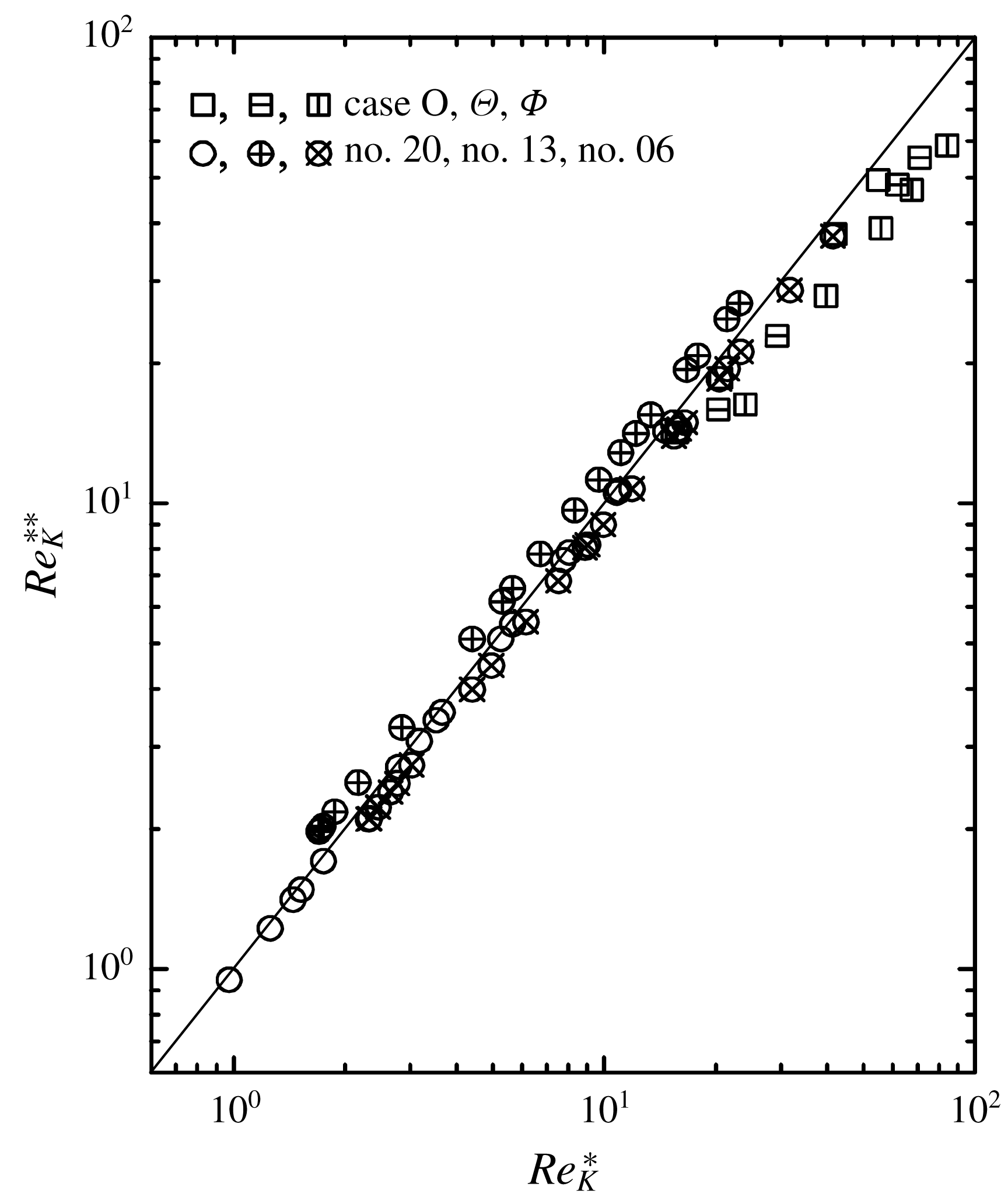
where
 $c$
is a constant to adjust the length scale. Interestingly, when
 $c=1/3.8$
is applied, an almost linear correlation between
 $Re_{K}^{\ast }$
and
 $Re_{K}^{\ast \ast }$
can be seen, as shown in figure 9. Note that when the surface pore is circular,
 $D_{p_{x}}$
is its diameter while for a non-circular pore case
 $D_{p_{x}}$
is simply defined as its streamwise length. Hence, for cases no. 20, no. 13 and no. 06,
 $D_{p_{x}}$
corresponds to their pore diameters 1.7, 2.8, 3.8 mm, respectively, while for cases O,
 $\unicode[STIX]{x1D6E9}$
and
 $\unicode[STIX]{x1D6F7}$
,
 $D_{p_{x}}=5~\text{mm}$
. Consequently, this surrogate permeability Reynolds number, which is essentially a kind of modified pore Reynolds number, may be used to characterize general porous medium cases. Table 2 also lists
 $Re_{K}^{\ast }$
and
 $Re_{K}^{\ast \ast }$
for the present cases.
Correlation between the generalized and surrogate permeability Reynolds numbers.

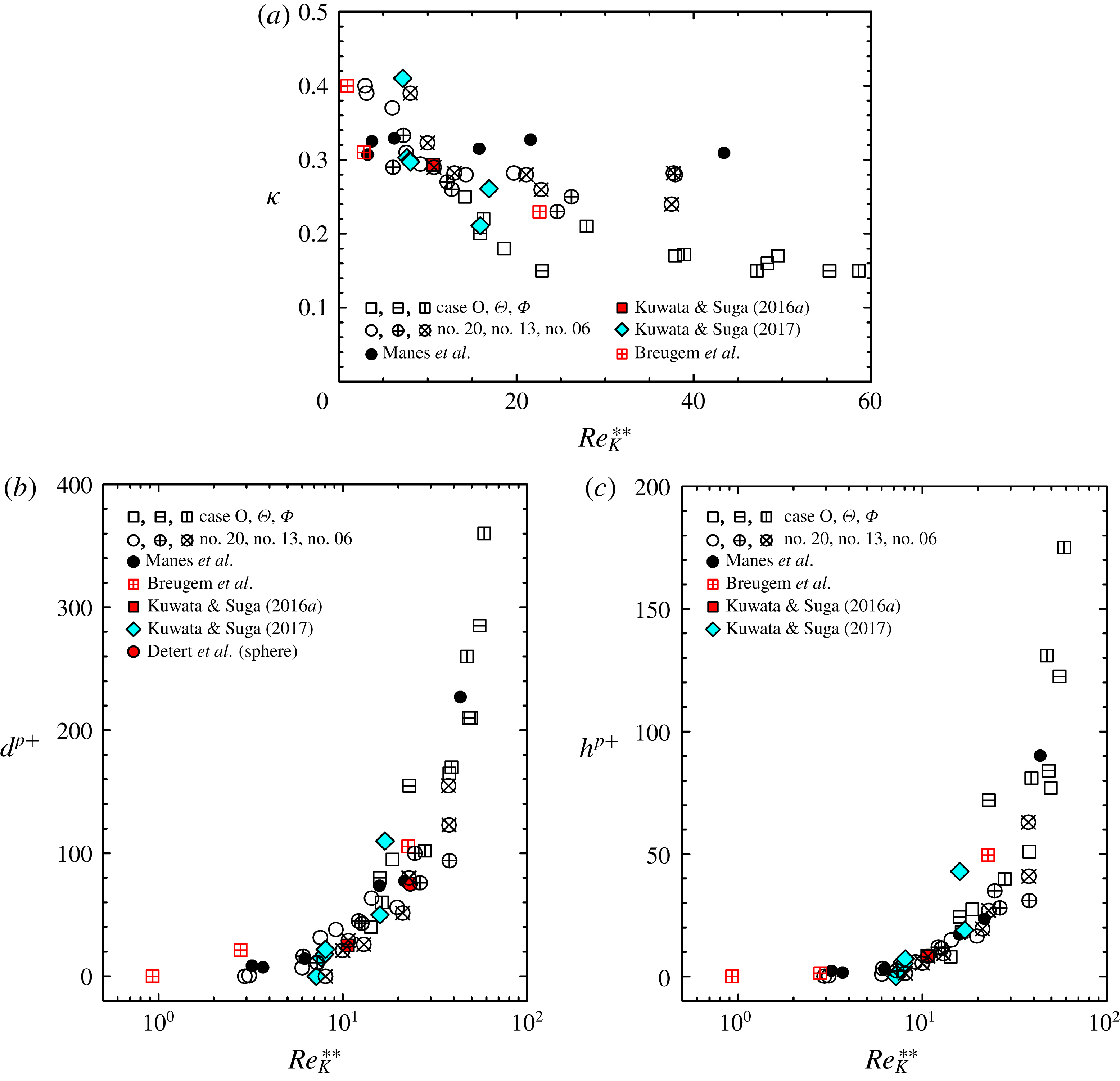
To confirm the applicability of this surrogate permeability Reynolds number
 $Re_{K}^{\ast \ast }$
to characterize the porous wall turbulence, figure 10 indicates all the data, including the isotropic porous medium cases of no. 20, no. 13 and no. 06 as well as the experimental data of Detert et al. (Reference Detert, Nikora and Jirka2010) and Manes et al. (Reference Manes, Poggi and Ridol2011) and numerical simulations of Breugem et al. (Reference Breugem, Boersma and Uittenbogaard2006) and Kuwata & Suga (Reference Kuwata and Suga2016a
, Reference Kuwata and Suga2017). For the cases of Breugem et al. (Reference Breugem, Boersma and Uittenbogaard2006) and Detert et al. (Reference Detert, Nikora and Jirka2010), porous media consisting of sphere grains were considered. Hence, the hydraulic diameter using the specific surface
 $a_{v}$
is applied as
 $D_{p_{x}}=4(\unicode[STIX]{x1D711}/a_{v}(1-\unicode[STIX]{x1D711}))$
. When the grain shape is spherical with diameter
 $D_{g}$
, the specific surface becomes
 $a_{v}=6/D_{g}$
. The plots in figure 10 show reasonable correlations between the parameters and
 $Re_{K}^{\ast \ast }$
for all the porous wall cases. Indeed, the data correlate well for the zero-plane displacement
 $d$
and the roughness scale
 $h$
although the plotted data for the von Kármán constant
 $\unicode[STIX]{x1D705}$
are again somewhat more scattered. Note that even though a couple of cases of Kuwata & Suga (Reference Kuwata and Suga2017) do not have the streamwise permeability,
 $Re_{K}^{\ast \ast }$
can be applied to those cases. It is thus suggested that the proposed surrogate permeability Reynolds number, equation (3.11), is promising for the general correlation parameter of turbulence over porous media.
Distributions of log-law parameters against the surrogate permeability Reynolds number
 $Re_{K}^{\ast \ast }$
: (a) von Kármán constant, (b) zero-plane displacement and (c) roughness scale. Data of Breugem et al. (Reference Breugem, Boersma and Uittenbogaard2006), Detert et al. (Reference Detert, Nikora and Jirka2010), Manes et al. (Reference Manes, Poggi and Ridol2011) and Kuwata & Suga (Reference Kuwata and Suga2016a
) are for isotropic porous media, data of Kuwata & Suga (Reference Kuwata and Suga2017) are for anisotropic porous media.

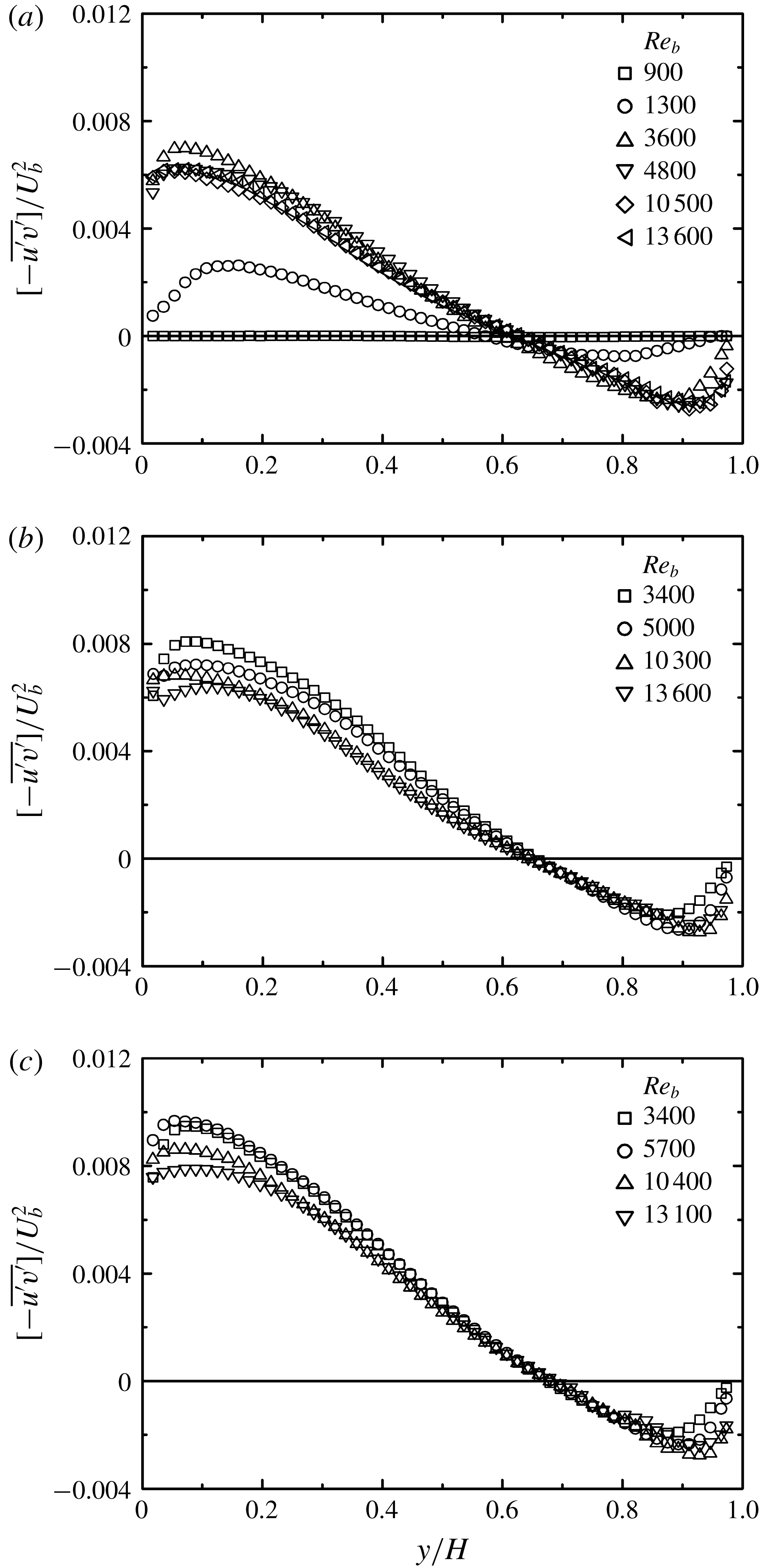
Comparison of Reynolds shear stress: (a) case O, (b) case
 $\unicode[STIX]{x1D6E9}$
, (c) case
 $\unicode[STIX]{x1D6F7}$
.

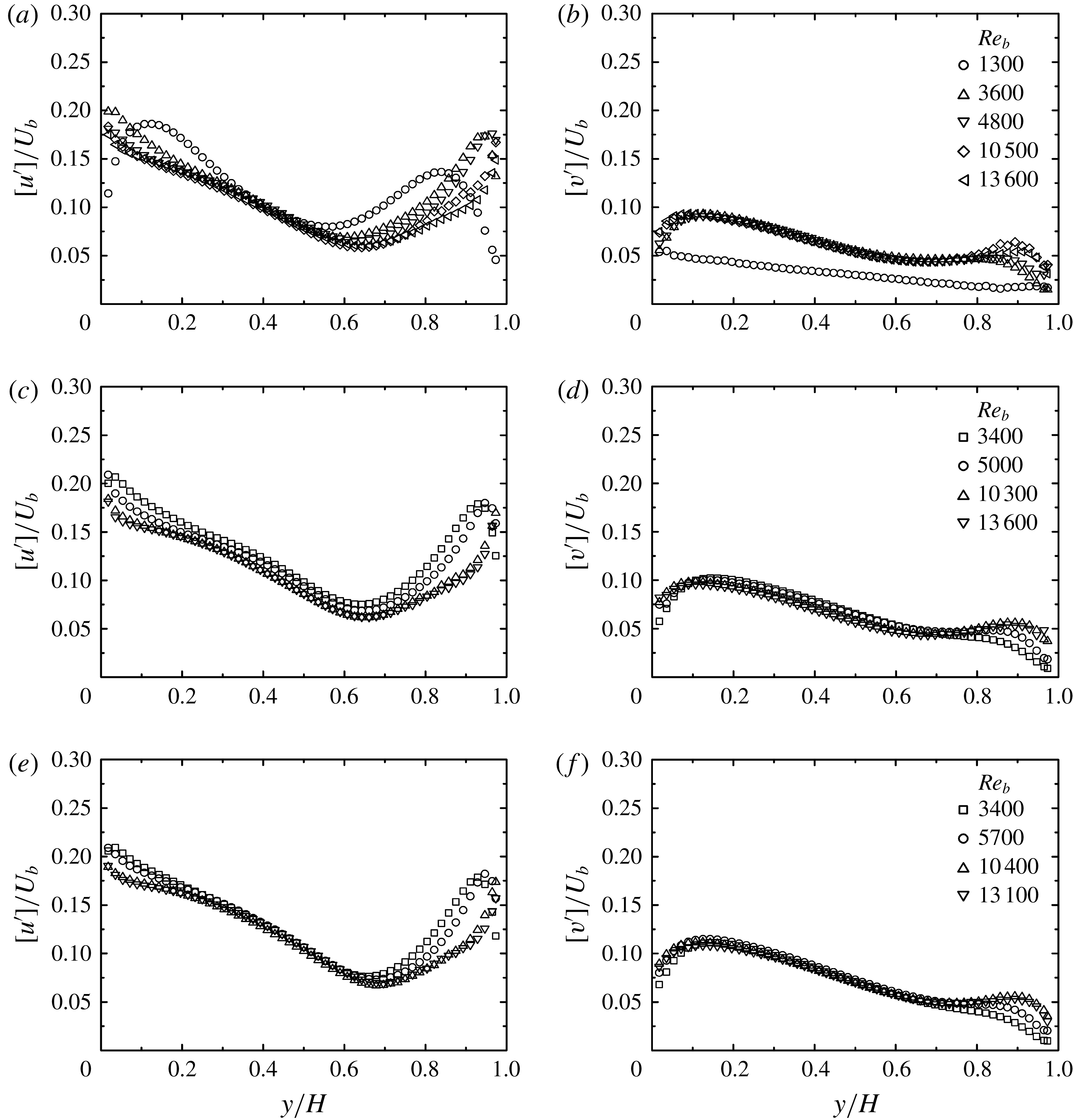
3.1.3 Turbulence quantities
Figure 11 compares the plane-averaged Reynolds shear stress
 $[-\overline{u^{\prime }v^{\prime }}]$
distribution profiles normalized by the bulk mean velocity
 $U_{b}$
to see the difference depending on the bulk Reynolds number. As confirmed in figure 11(a), in case O, the flow is laminar at
 $Re_{b}=900$
since
 $[-\overline{u^{\prime }v^{\prime }}]$
is almost zero across the channel. Then, at
 $Re_{b}=1300$
, the level of
 $[-\overline{u^{\prime }v^{\prime }}]$
increases, indicating that the laminar to turbulent transition is taking place, and the other profiles suggest that the transition is complete by
 $Re_{b}=3600$
. When the flow becomes turbulent, it is observed that the level of
 $[-\overline{u^{\prime }v^{\prime }}]$
near the porous wall (
 $y/H=0.0$
) becomes significantly higher than that near the solid top wall (
 $y/H=1.0$
). As seen in figure 11(b,c) for cases
 $\unicode[STIX]{x1D6E9}$
and
 $\unicode[STIX]{x1D6F7}$
, the trends at
 $Re_{b}\geqslant 3400$
look the same as that in case O. This confirms that the turbulence becomes significantly strong near the presently measured porous media. Corresponding to the trend of the plane-averaged Reynolds shear stress, turbulent intensities:
 $[u^{\prime }]$
and
 $[v^{\prime }]$
, which are the root-mean-square (r.m.s.) values of the plane-averaged Reynolds wall-normal stresses, generally become higher in the bottom half of the channel than in the top half of the channel, as seen in figure 12. Particularly,
 $[v^{\prime }]$
near the porous wall is considerably higher than near the top wall. Due to the relaxed wall-blocking effect by the porous surfaces,
 $[\overline{{v^{\prime }}^{2}}]$
has larger values near the porous medium than near the solid wall, leading to the enhancement of the production of the plane-averaged Reynolds shear stress,
 $-[\overline{{v^{\prime }}^{2}}]\unicode[STIX]{x2202}[U]/\unicode[STIX]{x2202}y$
. Accordingly, the turbulence level near the porous walls becomes high. This is the main reason why the turbulence level becomes high near the porous medium in many studies (e.g. Lovera & Kennedy Reference Lovera and Kennedy1969; Ruff & Gelhar Reference Ruff and Gelhar1972; Ho & Gelhar Reference Ho and Gelhar1973; Zagni & Smith Reference Zagni and Smith1976; Kong & Schetz Reference Kong and Schetz1982; Zippe & Graf Reference Zippe and Graf1983; Breugem et al.
Reference Breugem, Boersma and Uittenbogaard2006; Suga et al.
Reference Suga, Matsumura, Ashitaka, Tominaga and Kaneda2010). However, when the slip velocity on the porous wall becomes much higher than the present ones due to higher porosity and/or permeability, the velocity gradient
 $\unicode[STIX]{x2202}[U]/\unicode[STIX]{x2202}y$
is expected to be considerably relaxed and this damps turbulence generation. In fact, in the rigid-vegetation-canopy flows of Nezu & Sanjou (Reference Nezu and Sanjou2008), the friction velocity at
 $\unicode[STIX]{x1D711}=0.99$
reduced to 84 % of that at
 $\unicode[STIX]{x1D711}=0.97$
, while it could not be confirmed which parameter controlled this trend since the permeabilities were unknown. In any case, although the relation between the surface turbulence and the porous parameters is considered to be non-monotonic, the present cases are in the range of turbulence enhancement.
Comparison of turbulent intensities: (a) streamwise turbulent intensity of case O, (b) wall-normal turbulent intensity of case O, (c) streamwise turbulent intensity of case
 $\unicode[STIX]{x1D6E9}$
, (d) wall-normal turbulent intensity of case
 $\unicode[STIX]{x1D6E9}$
, (e) streamwise turbulent intensity of case
 $\unicode[STIX]{x1D6F7}$
, (f) wall-normal turbulent intensity of case
 $\unicode[STIX]{x1D6F7}$
.

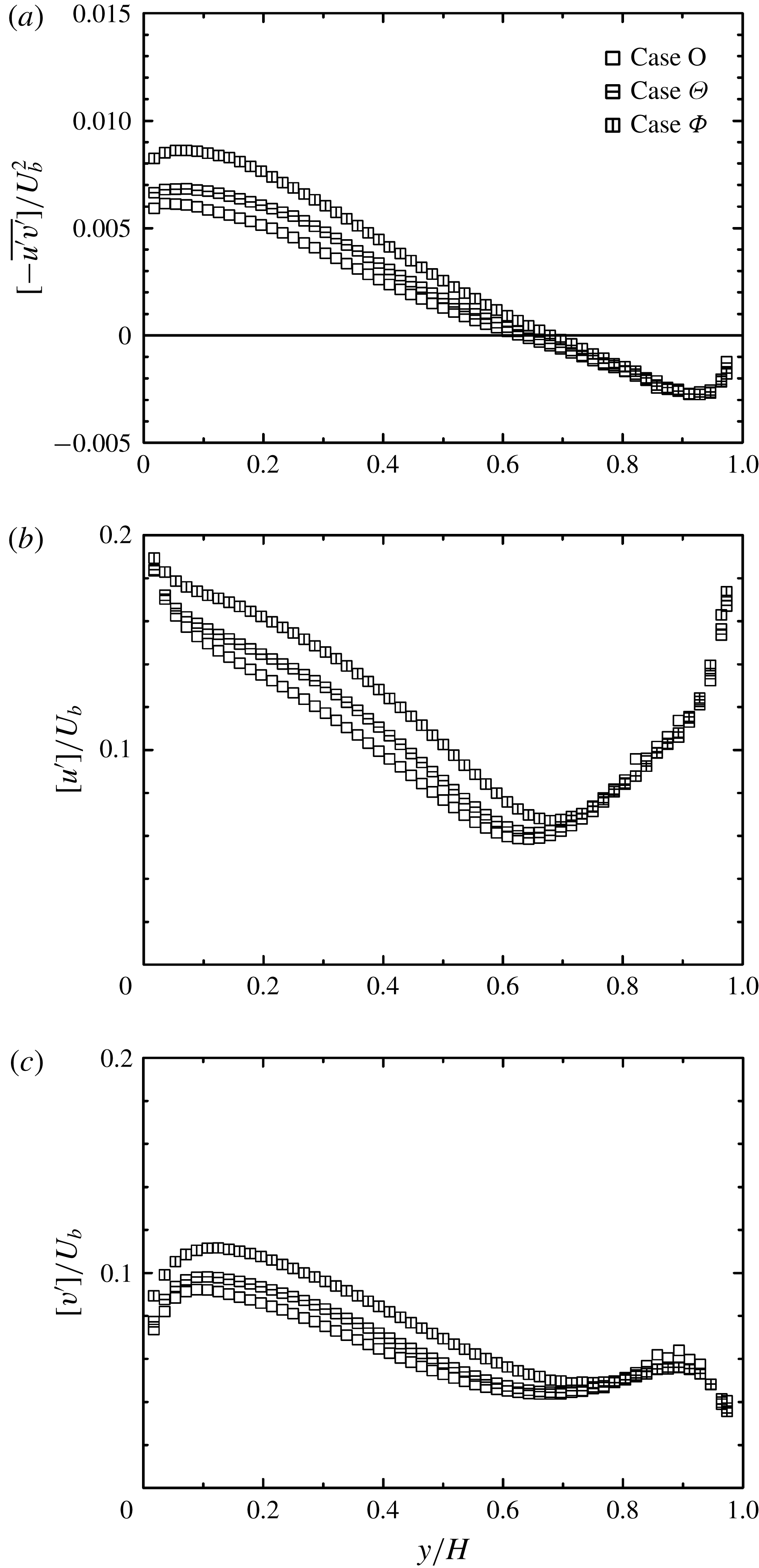
Comparison of turbulence quantities at
 $Re_{b}\simeq 10\,500$
: (a) Reynolds shear stress, (b) streamwise turbulent intensity, (c) wall-normal turbulent intensity.

Since the porosity is constant at
 $\unicode[STIX]{x1D711}=0.7$
in the present cases, it is possible to see the effects of the permeability. Figure 13 compares the plane-averaged Reynolds shear stress and turbulent intensity profiles at
 $Re_{b}\simeq 10\,500$
. Near the porous wall it is seen that case
 $\unicode[STIX]{x1D6F7}$
is most turbulent and the least turbulent one is case O, although its wall-normal permeability
 $\unicode[STIX]{x1D612}_{yy}$
is approximately two orders of magnitude larger than the other cases. This indicates that, although permeable surfaces relax the near-wall blocking effect on vortex motions and lead to strong turbulence, turbulence generation in the present cases is not very sensitive to the wall-normal permeability
 $\unicode[STIX]{x1D612}_{yy}$
. Interestingly, rather than
 $\unicode[STIX]{x1D612}_{yy}$
, a small difference in
 $\unicode[STIX]{x1D612}_{xx}$
seems to affect turbulence generation. (This trend does not change in the different
 $Re_{b}$
cases.) Indeed, case
 $\unicode[STIX]{x1D6F7}$
, whose
 $\unicode[STIX]{x1D612}_{xx}$
is 25 % larger than that of case
 $\unicode[STIX]{x1D6E9}$
, is the most turbulent, and case O, whose
 $\unicode[STIX]{x1D612}_{xx}$
is 25 % smaller than that of case
 $\unicode[STIX]{x1D6E9}$
, is the least turbulent. When the ratio between the wall-normal and streamwise permeabilities is considered, the present cases are at
 $\unicode[STIX]{x1D612}_{yy}/\unicode[STIX]{x1D612}_{xx}=1.2$
, 1.5 and 172.7. Thus, there might be a question about whether those trends are monotonic between the ratios of 1.5 and 172.7. Although the channel geometry was not the same as the present one, Matsuo et al. (Reference Matsuo, Okabe, Kaneda and Suga2017) applied orthotropic porous media whose permeabilities were
 $(\unicode[STIX]{x1D612}_{xx},\unicode[STIX]{x1D612}_{yy},\unicode[STIX]{x1D612}_{zz})=(0.22,0.17,0.22)$
and
 $(0.16,0.97,0.16)~\text{mm}^{2}$
to the bottom wall of turbulent rectangular duct flows and reported that turbulence was sensitive to the streamwise permeability rather than the wall-normal permeability. Their permeability ratios were
 $\unicode[STIX]{x1D612}_{yy}/\unicode[STIX]{x1D612}_{xx}=0.77$
and 6.1. Hence, although the supporting data might not be sufficient, we consider that the presently observed trends are monotonic in the range of
 $\unicode[STIX]{x1D612}_{yy}/\unicode[STIX]{x1D612}_{xx}=0.77{-}172.7$
.
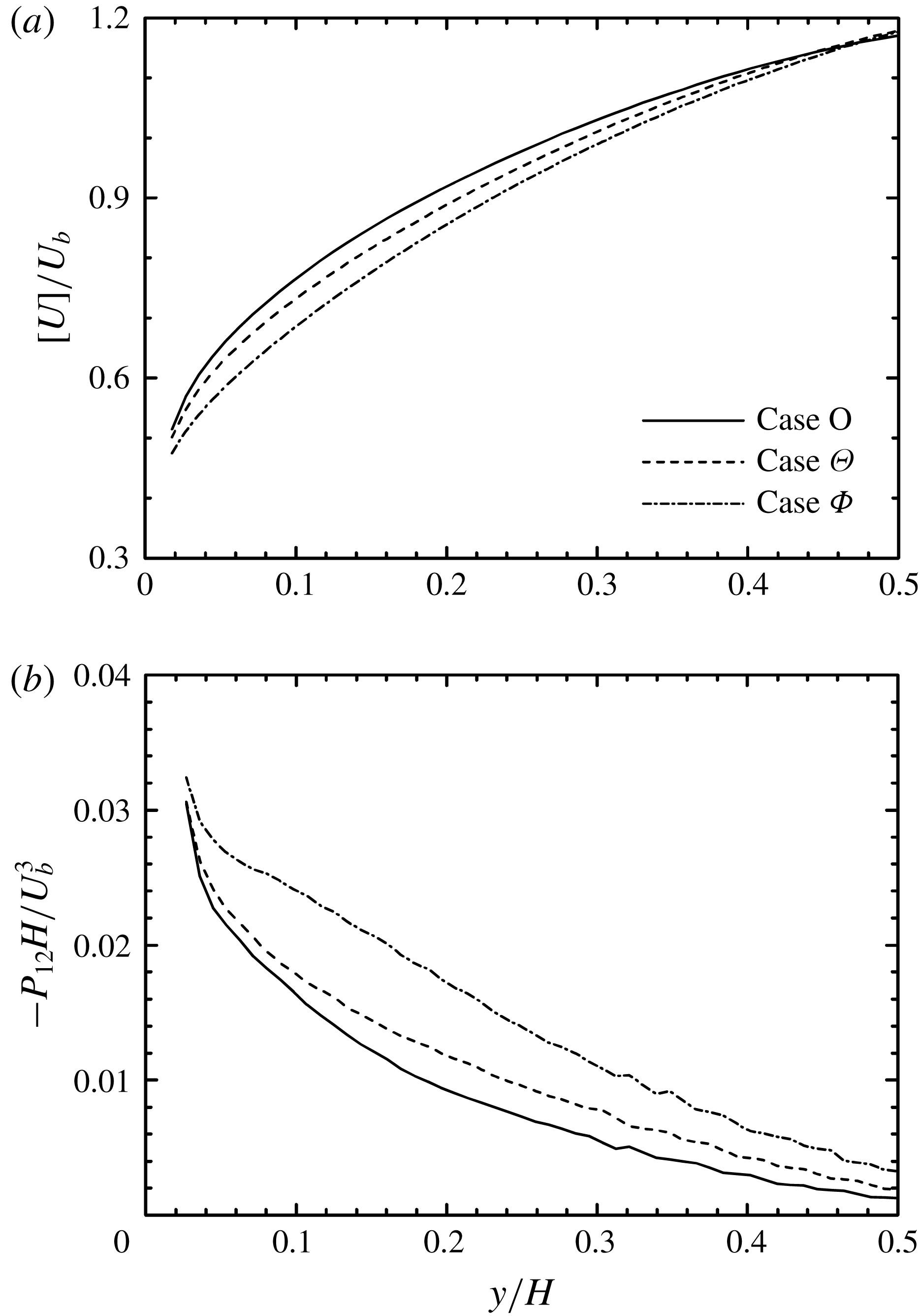
Comparison of mean velocity and shear production near the porous wall at
 $Re_{b}\simeq 10\,500$
: (a) mean velocity profiles, (b) shear production
 $P_{12}=-[\overline{{v^{\prime }}^{2}}]\unicode[STIX]{x2202}[U]/\unicode[STIX]{x2202}y$
profiles.

For the flow underneath the porous surface, equation (3.7) suggests that the drag reduces as the streamwise permeability increases. Accordingly, the increase of
 $\unicode[STIX]{x1D612}_{xx}$
leads to an increased flow rate, enhancing the slippage velocity on the surface. This results in a more relaxed shear rate
 $\unicode[STIX]{x2202}[U]/\unicode[STIX]{x2202}y$
near the surface. This is confirmed in figure 14(a) which compares near-wall velocity profiles at
 $Re_{b}\simeq 10\,500$
. Case O shows the largest velocity gradient, followed by case
 $\unicode[STIX]{x1D6E9}$
and then case
 $\unicode[STIX]{x1D6F7}$
. Consequently, for the present cases, it is considered that relaxing the wall-blocking effect on turbulence enhances turbulence generation significantly, making up for the reduction by relaxing the velocity gradient. Indeed, as shown in figure 14(b), the profile of shear production
 $P_{12}=-[\overline{{v^{\prime }}^{2}}]\unicode[STIX]{x2202}[U]/\unicode[STIX]{x2202}y$
of case
 $\unicode[STIX]{x1D6F7}$
shows the largest level, followed by those of cases
 $\unicode[STIX]{x1D6E9}$
and O. Accordingly, although it might be expected that relaxing the wall-blocking effect is related to the wall-normal permeability, turbulence generation is not controlled by the wall-normal permeability.
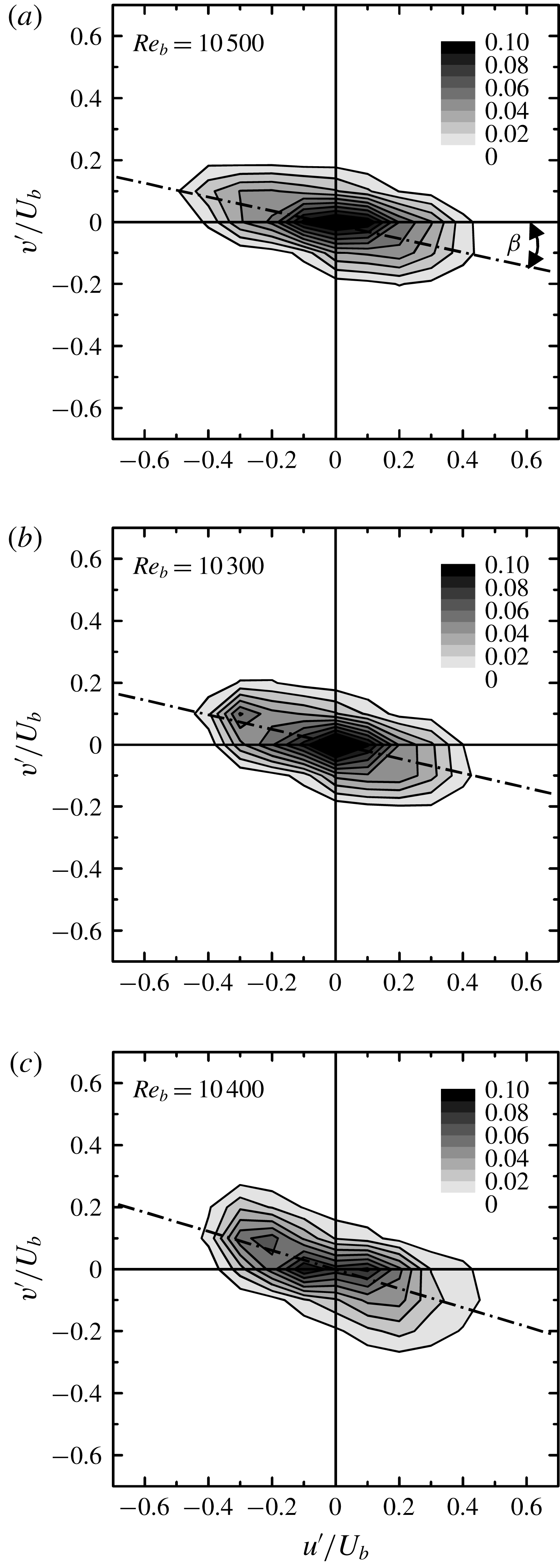
To see the near-wall turbulence in more detail, figure 15 shows the distribution of the joint probability density function
 $p(u^{\prime },v^{\prime })$
at
 $y^{p+}=15$
for
 $Re_{b}\simeq 10\,500$
. Although the shape difference is not very drastic, the angles between the major and the streamwise axes are
 $\unicode[STIX]{x1D6FD}=11.9^{\circ }$
,
 $12.2^{\circ }$
and
 $16.4^{\circ }$
for cases O,
 $\unicode[STIX]{x1D6E9}$
and
 $\unicode[STIX]{x1D6F7}$
, respectively. The order of the angle magnitude corresponds to the order of
 $\unicode[STIX]{x1D612}_{xx}$
. Here, the major axis is determined as the least-squares approximated line of plots of
 $(u^{\prime },v^{\prime })$
. When the motions in the second and fourth quadrants (Q2 and Q4) simultaneously have large streamwise and wall-normal fluctuations,
 $\unicode[STIX]{x1D6FD}$
increases and thus
 $\unicode[STIX]{x1D6FD}$
is a measure of the strength of the wall-normal fluctuations. Interestingly, even though the wall-normal permeability is approximately two orders of magnitude larger than the other cases, case O has the smallest
 $\unicode[STIX]{x1D6FD}$
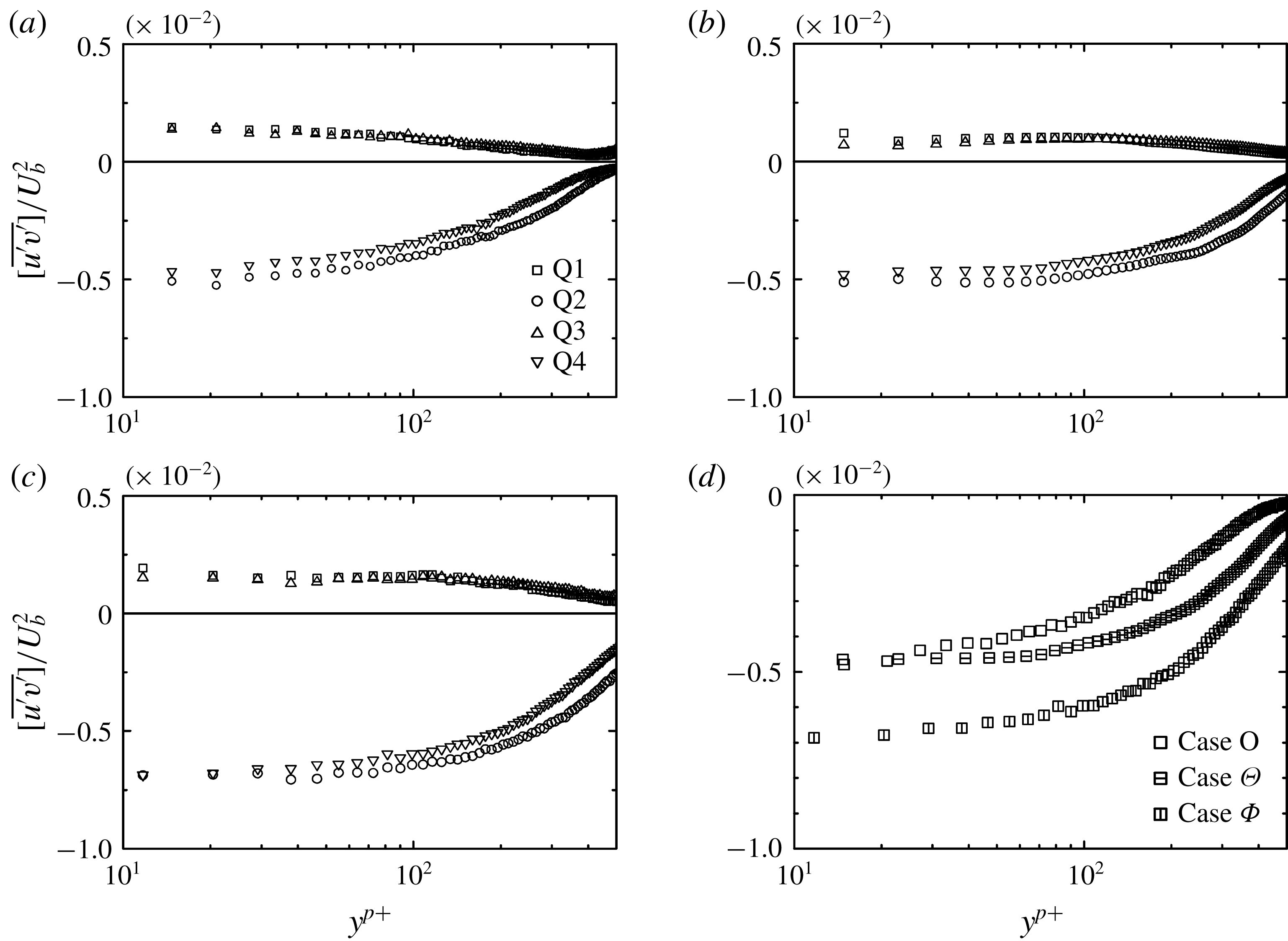
, suggesting that its near-wall turbulence receives more the wall-blocking effect. For further discussion, the decomposed Reynolds shear stress profiles are investigated using the quadrant analysis method:
 $$\begin{eqnarray}\displaystyle \overline{(uv)}_{m}=\frac{1}{\displaystyle \sum N_{m}}\sum (u^{\prime }v^{\prime })_{m}, & & \displaystyle\end{eqnarray}$$
where subscript
 $m~(=1{-}4)$
corresponds to the quadrant event. Figure 16(a–c) compares the decomposed Reynolds shear stress profiles of cases O,
 $\unicode[STIX]{x1D6E9}$
and
 $\unicode[STIX]{x1D6F7}$
at
 $Re_{b}\simeq 10\,500$
. In all the plots, it is obvious that the events of the second quadrant (Q2), ejections, are dominant. The fourth quadrant (Q4), which corresponds to sweeps, is also larger and tends to be nearly the same as Q2 as the position moves toward the wall surface. For turbulence near a solid wall, Wallace, Eckelmann & Brodkey (Reference Wallace, Eckelmann and Brodkey1972) reported that Q4 was dominant very close to the wall while Q2 overtook it as the location moved away from the wall. The previous study on isotropic porous media (Suga et al.
Reference Suga, Mori and Kaneda2011) also showed such a trend and the intersection points of Q2 and Q4 were at
 $y^{p+}=30{-}100$
for
 $Re_{b}\simeq 10\,000$
. However, the present cases only show the distributions after the intersections (if they exist). As seen in figure 16(d), which compares the Q4 distributions, obviously the Q4 profile of case
 $\unicode[STIX]{x1D6F7}$
is most negative. The levels of cases O and
 $\unicode[STIX]{x1D6E9}$
are similar to each other close to the wall while that of case
 $\unicode[STIX]{x1D6E9}$
becomes more negative away from the wall. This suggests that sweep motions tend to extend more away from the wall with the increase of the streamwise permeability. Since parts of wall penetrating vortices having large streamwise momentum are observed as sweeps, the streamwise permeability becomes the primary factor to maintain strong near-wall rotating motions when the wall-normal permeability is sufficiently large. Because the wall penetrating fluid pushes out the same amount of fluid from the surface forming parts of the ejections, the profiles of the ejections are closely related to those of the sweeps. Therefore, the sweeps and the ejections are considerably affected by the streamwise permeability. This is one of the reasons why turbulence appears to be controlled by the streamwise permeability in this study. However, when the permeability ratio becomes smaller,
 $\unicode[STIX]{x1D612}_{yy}/\unicode[STIX]{x1D612}_{xx}\ll 1.0$
, a different trend might be observed.
Joint probability density function
 $p(u^{\prime },v^{\prime })$
of fluctuating velocity at
 $y^{p+}=15$
for
 $Re_{b}\simeq 10\,500$
: (a) case O (
 $\unicode[STIX]{x1D6FD}=11.9^{\circ }$
), (b) case
 $\unicode[STIX]{x1D6E9}$
(
 $\unicode[STIX]{x1D6FD}=12.2^{\circ }$
), (c) case
 $\unicode[STIX]{x1D6F7}$
(
 $\unicode[STIX]{x1D6FD}=16.4^{\circ }$
);
 $\unicode[STIX]{x1D6FD}$
is the streamwise angle of the major axis of the
 $(u^{\prime },v^{\prime })$
distribution.

Quadrant analysis of the Reynolds shear stress distributions at
 $Re_{b}\simeq 10\,500$
: (a) case O at
 $Re_{b}=10\,500$
, (b) case
 $\unicode[STIX]{x1D6E9}$
at
 $Re_{b}=10\,300$
, (c) case
 $\unicode[STIX]{x1D6F7}$
at
 $Re_{b}=10\,400$
, (d) comparison of sweeps, Q4.

3.2 Streamwise–spanwise plane measurements
To understand the turbulence fields in greater detail, streamwise–spanwise plane measurements are carried out and the spanwise structure is discussed. With the present experimental facility and measurement method, the two-dimensionality of the flow field and the reproducibility of the data between the
 $x$
–
 $y$
and
 $x$
–
 $z$
measurements are well confirmed, as mentioned in § 2. The measured flows are at
 $Re_{b}=3600$
, 4800, 10 500, 13 600 for case O,
 $Re_{b}=3400$
, 5000, 10 300, 13 600 for case
 $\unicode[STIX]{x1D6E9}$
and
 $Re_{b}=3400$
, 5700, 10 400, 13 100 for case
 $\unicode[STIX]{x1D6F7}$
.
3.2.1 Snapshots of turbulence fields
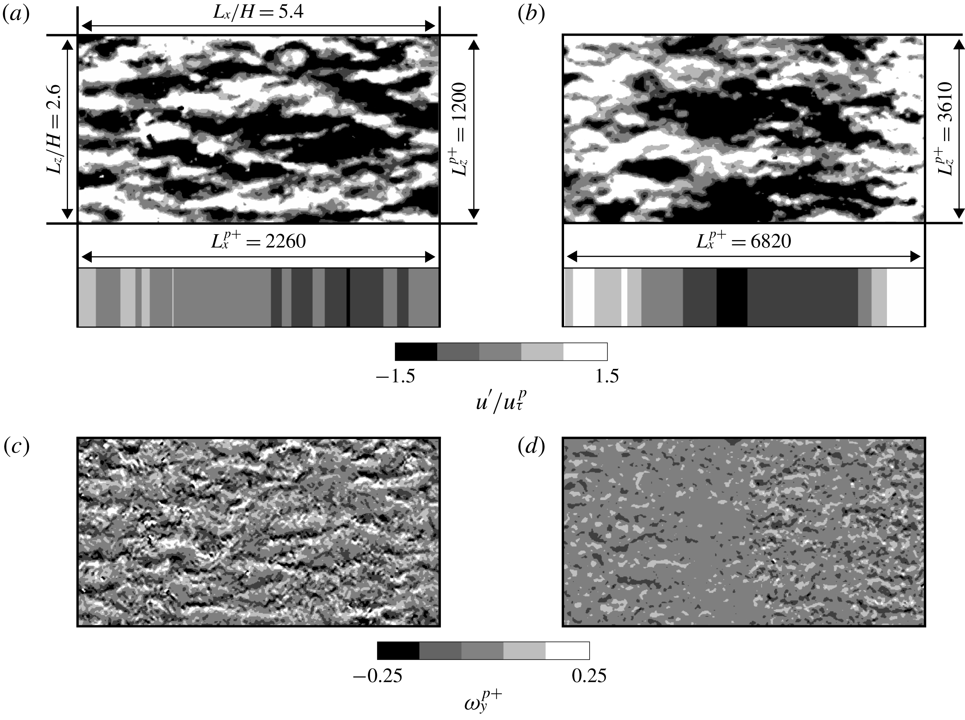
Figure 17(a,b) shows examples of snapshots of the instantaneous streamwise velocity fluctuation
 $u^{\prime }$
indicating low- and high-speed fluid lumps observed at
 $y^{p+}\simeq 20$
for case O at
 $Re_{b}=4800$
(
 $Re_{K}^{\ast }=20.6$
) and case
 $\unicode[STIX]{x1D6F7}$
at
 $Re_{b}=13\,100$
(
 $Re_{K}^{\ast }=83.8$
), respectively. The window size is
 $L_{x}/H\times L_{z}/H=5.4\times 2.6$
, which corresponds to
 $L_{x}^{p+}\times L_{z}^{p+}=2260\times 1200$
and
 $L_{x}^{p+}\times L_{z}^{p+}=6820\times 3610$
, respectively, for figure 17(a,b). Clearly, large scale low- and high-speed fluid lumps are observed. The corresponding vorticity fields are shown in figure 17(c,d). In figure 17(c), there are fragments of shredded vortex tubes looking similar to those observed at a location under the structural transition range in the isotropic porous medium cases (Suga et al.
Reference Suga, Nakagawa and Kaneda2017). This suggests that the condition of figure 17(a,c) is still under the transition range that is discussed later in § 3.2.2. Compared with figure 17(a), the fluid lumps look well aligned in the spanwise direction in figure 17(b). Their length
 $\times$
width is approximately
 $\unicode[STIX]{x0394}x^{p+}\times \unicode[STIX]{x0394}z^{p+}=5000\times 1300$
. The observed patterns are very different from the longitudinally elongated streaks usually detected over solid smooth walls. Similar large-scale fluid lumps were also observed in the isotropic porous medium cases over the transitional range and such patterns of fluid lumps were considered to be footprints of the spanwise transverse rolls, which are considered to be generated by the K–H instability. Jiménez et al. (Reference Jiménez, Uhlmann, Pinelli and Kawahara2001) suggested that a large-scale perturbation is induced by the K–H instability associated with an inflection point of the mean velocity profile at the surface of the porous layer. In fact, the vorticity patterns seen in figure 17(d) look more regularly arranged and very similar to those indicated by the simulation of Kuwata & Suga (Reference Kuwata and Suga2017). Since the pores of the present porous media are aligned with the coordinate axes as in the simulation, the footprints can be maintained more visibly than in the isotropic porous medium cases.
Snapshots of low- and high-speed fluid lumps at
 $y^{p+}\simeq 20$
: (a,b) fluctuation velocity contours of case O at
 $Re_{b}=4800,Re_{K}^{\ast }=20.6$
and case
 $\unicode[STIX]{x1D6F7}$
at
 $Re_{b}=13\,100,Re_{K}^{\ast }=83.8$
, respectively. The upper images are snapshots of the instantaneous fields and the lower images correspond to the spanwise-averaged fields of the upper images. (c,d) Instantaneous wall-normal vorticity
 $\unicode[STIX]{x1D714}_{y}^{p+}=(\unicode[STIX]{x2202}u/\unicode[STIX]{x2202}z-\unicode[STIX]{x2202}w/\unicode[STIX]{x2202}x)\unicode[STIX]{x1D708}/(u_{\unicode[STIX]{x1D70F}}^{p})^{2}$
fields corresponding to the snapshots shown in (a) and (b), respectively.

Two-point correlation of the streamwise velocity versus spanwise spacing: (a) case O at
 $Re_{b}=4800$
(
 $Re_{K}^{\ast }=20.6$
), (b) case
 $\unicode[STIX]{x1D6E9}$
at
 $Re_{b}=10\,300$
(
 $Re_{K}^{\ast }=61.9$
), (c) case
 $\unicode[STIX]{x1D6F7}$
at
 $Re_{b}=13\,100$
(
 $Re_{K}^{\ast }=83.8$
).

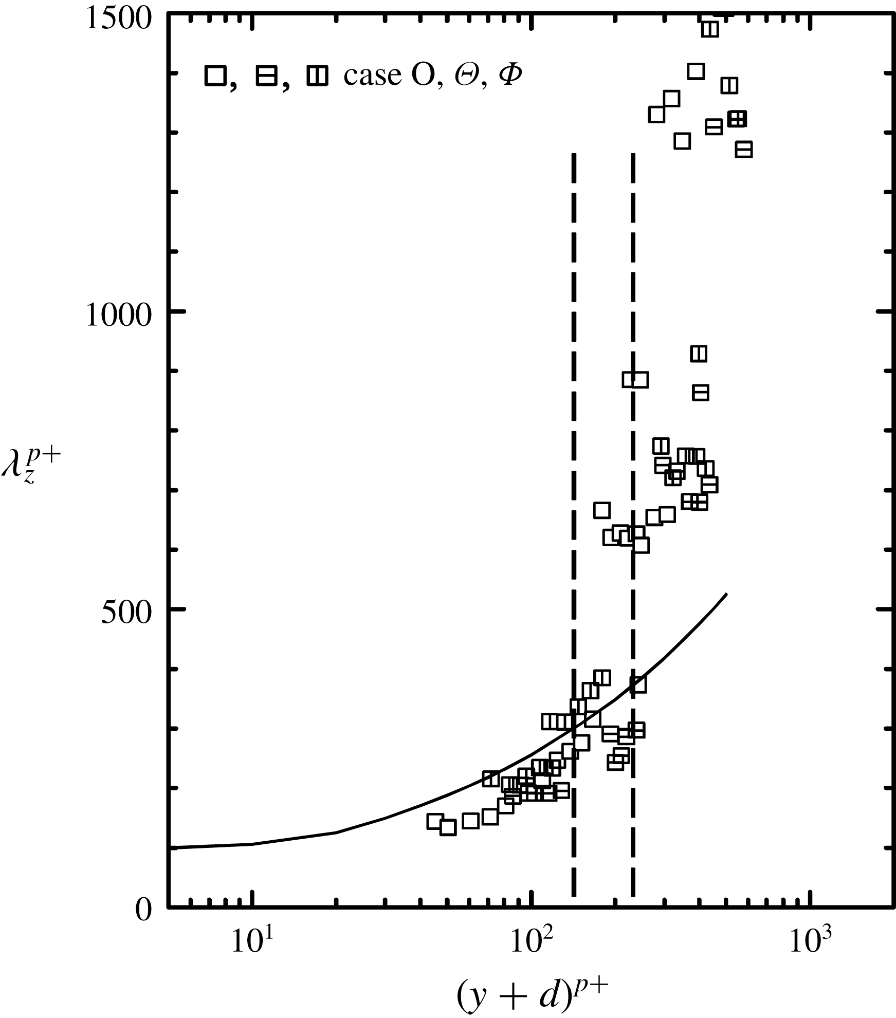
Distribution of spanwise spacing of streaks in the wall-normal direction. The solid line indicates the fitting line of the solid wall cases from the literature (Smith & Metzler Reference Smith and Metzler1983; Iritani, Kasagi & Hirata Reference Iritani, Kasagi and Hirata1985; Kim, Moin & Moser Reference Kim, Moin and Moser1987; Tomkins & Adrian Reference Tomkins and Adrian2003) and dashed lines indicate the transitional range.

3.2.2 Two-point correlations
The normalized two-point correlation function
 $$\begin{eqnarray}\displaystyle \widehat{\unicode[STIX]{x1D619}_{ij}}(\unicode[STIX]{x0394}z)=\frac{\unicode[STIX]{x1D619}_{ij}(\unicode[STIX]{x0394}z)}{\unicode[STIX]{x1D619}_{ij}(0)}=\frac{\overline{u_{i}^{\prime }(z)u_{j}^{\prime }(z+\unicode[STIX]{x0394}z)}}{\overline{u_{i}^{\prime }(z)u_{j}^{\prime }(z)}} & & \displaystyle\end{eqnarray}$$
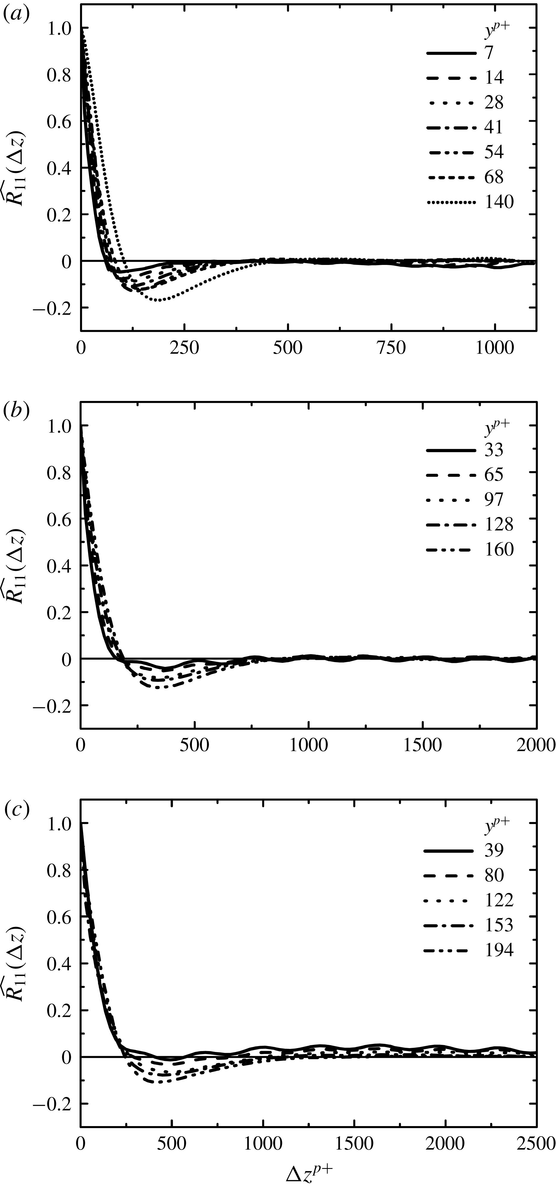
in the spanwise direction is applied to detect the spanwise scales of the structure. Figure 18 shows examples of
 $\widehat{R_{11}}(\unicode[STIX]{x0394}z)$
distributions. Figure 18(a–c) corresponds to the results of case O at
 $Re_{b}=4800$
, case
 $\unicode[STIX]{x1D6E9}$
at
 $Re_{b}=10\,300$
and case
 $\unicode[STIX]{x1D6F7}$
at
 $Re_{b}=13\,100$
, respectively. Although they are not very clear in figure 18(a), the distribution indicates short wavy profiles at locations closer to the wall surface, as clearly shown in figure 18(b,c) for the higher Reynolds numbers. It has been confirmed that the wavelength of those short waves corresponds to the pore pitch of the EVA net shown in figure 1(a). However, as the wall-normal distance increases, those short waves disappear and local minimum in the profile becomes clearer. The depth of the local minimum and its positions change depending on the wall-normal distance. The locations of those local minima indicate the statistical spanwise distance between low-speed and neighbouring high-speed flow regions. Figure 19 shows the distributions of the spanwise spacing of streaks
 $\unicode[STIX]{x1D706}_{z}^{p+}$
against the wall-normal distance plus the zero-plane displacement
 $d$
with a curve that indicates the fitting line of the smooth solid wall cases obtained from the literature (Smith & Metzler Reference Smith and Metzler1983; Iritani et al.
Reference Iritani, Kasagi and Hirata1985; Kim et al.
Reference Kim, Moin and Moser1987; Tomkins & Adrian Reference Tomkins and Adrian2003). Since the zero-plane displacement is a length scale associated with the penetration,
 $(y+d)^{p+}$
is an equivalent height to
 $y^{+}$
of smooth solid wall turbulence. It is seen that the points of
 $\unicode[STIX]{x1D706}_{z}^{p+}$
collapse around the curve under
 $(y+d)^{p+}=150{-}200$
reasonably well. In the isotropic porous medium cases,
 $\unicode[STIX]{x1D706}_{z}^{p+}$
also collapsed around the curve under
 $(y+d)^{p+}\simeq 100$
(Suga et al.
Reference Suga, Nakagawa and Kaneda2017). They concluded that although the coherent streaky structure was disturbed, its characteristics were still maintained in such a region. This suggests that, as seen in figure 17(c) whose location corresponds to
 $(y+d)^{p+}\simeq 105$
, the structure observed in the present study may retain some of the characteristics of the coherent streaky structure at such a location, which is a little higher than that of the isotropic porous medium case. At a position over a certain distance from the wall surfaces of
 $(y+d)^{p+}=150{-}200$
, the plotted values start to deviate significantly from the correlation line. Above this structural transition region, the quasi-streaky structure is smeared out and no longer exists, as can also be confirmed in figure 17(d), whose location corresponds to
 $(y+d)^{p+}\simeq 380$
. Since, as discussed in § 3.1.2, the zero-plane displacement
 $d$
has a correlation with the generalized permeability Reynolds number
 $Re_{K}^{\ast }$
(and the surrogate permeability Reynolds number
 $Re_{K}^{\ast \ast }$
), the observed structural change certainly correlates with the streamwise permeability.
Two-point correlation of the streamwise velocity versus streamwise spacing: (a) standard two-point correlation functions
 $\widehat{R_{11}}(\unicode[STIX]{x0394}x)$
for case
 $\unicode[STIX]{x1D6E9}$
at
 $Re_{b}=10\,300$
(
 $Re_{K}^{\ast }=61.9$
), (b) standard two-point correlation functions
 $\widehat{R_{11}}(\unicode[STIX]{x0394}x)$
for case
 $\unicode[STIX]{x1D6F7}$
at
 $Re_{b}=13\,100$
(
 $Re_{K}^{\ast }=83.8$
), (c) two-point correlation functions of the spanwise-averaged field
 $\widehat{\langle R_{11}\rangle }_{z}(\unicode[STIX]{x0394}x)$
for case
 $\unicode[STIX]{x1D6E9}$
at
 $Re_{b}=10\,300$
, (d) two-point correlation functions of the spanwise-averaged field
 $\widehat{\langle R_{11}\rangle }_{z}(\unicode[STIX]{x0394}x)$
for case
 $\unicode[STIX]{x1D6F7}$
at
 $Re_{b}=13\,100$
.

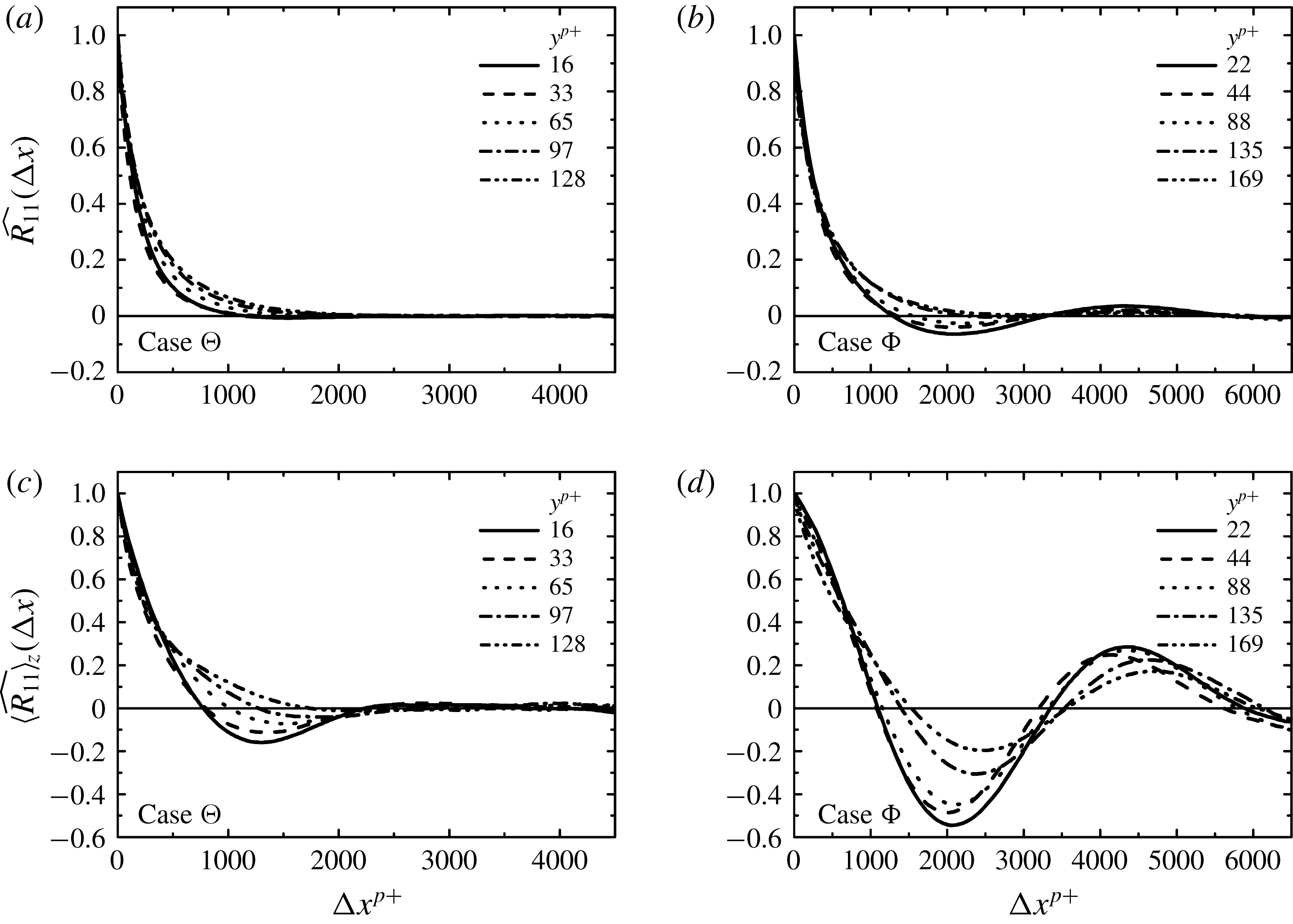
For the discussion of the streamwise length of the fluid lumps, figure 20(a,b) shows examples of the distribution profiles of
 $\widehat{R_{11}}(\unicode[STIX]{x0394}x)$
. Although it is possible to detect the local minima and maxima of the profiles in some cases, as seen in figure 20(b), generally it is impossible to do so, as seen in figure 20(a). This is because some small fluid lumps are irregularly detected between large fluid lumps and hence the averaging blurs their correlation
 $u_{i}^{\prime }(x)u_{j}^{\prime }(x+\unicode[STIX]{x0394}x)$
. It can be considered that a part of those fluid lumps is produced by the instability with high wavenumber motions. By performing a linear stability analysis on free surface flows over porous media, Camporeale, Mantelli & Manes (Reference Camporeale, Mantelli and Manes2013) classified the instability modes into three categories: namely, the surface, shear and porosity induced modes. In the porosity induced instability mode, there are three sub-categories: stable, unstable and that caused by the interaction with the free surface. Although detecting the waves of these instability modes by spectral analysis is desirable, it is impossible at the present sampling rate of 4 Hz. Accordingly, we focus on detecting the lowest streamwise wavenumber motions, which may correspond to the surface mode, by a two-point correlation function of the spanwise-averaged fluctuating velocities. Its definition is
 $$\begin{eqnarray}\displaystyle \widehat{\langle \unicode[STIX]{x1D619}_{ij}\rangle }_{z}(\unicode[STIX]{x0394}x)=\frac{\overline{\langle u_{i}^{\prime }(x)\rangle _{z}\langle u_{j}^{\prime }(x+\unicode[STIX]{x0394}x)\rangle }_{z}}{\overline{\langle u_{i}^{\prime }(x)\rangle _{z}\langle u_{j}^{\prime }(x)\rangle }_{z}}, & & \displaystyle\end{eqnarray}$$
where
 $\langle u_{i}^{\prime }(x)\rangle _{z}$
is the spanwise averaged instantaneous fluctuating velocity. By this process, the contribution from the noisy smaller fluid lumps is reasonably damped. See the samples of the spanwise-averaged fluctuating velocities in the lower images of figure 17(a,b).
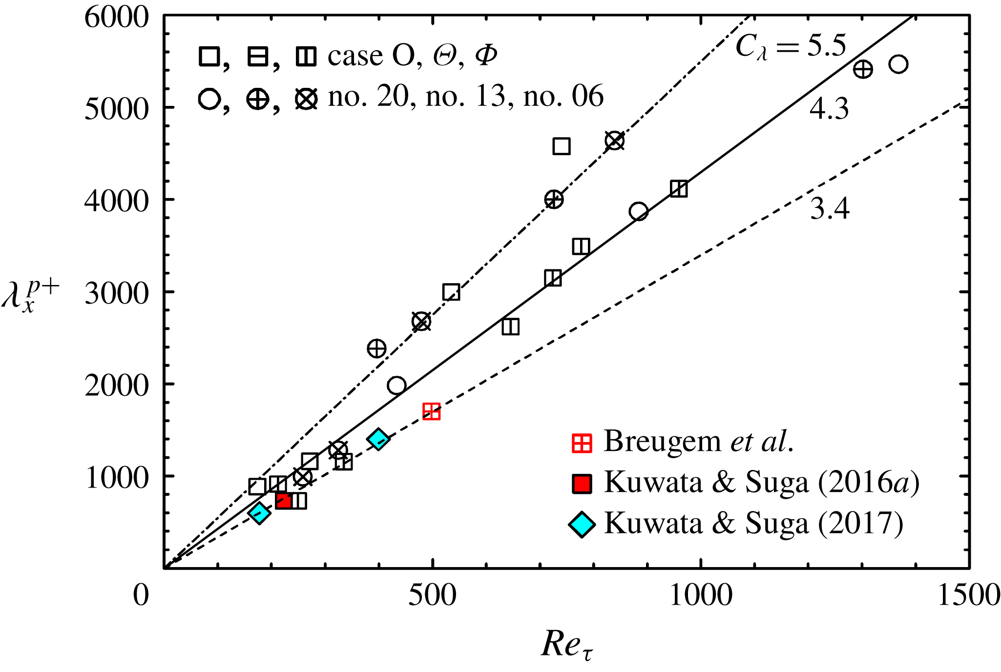
Streamwise wavelength of the fluid lumps: no. 20, no. 13 and no. 06 are the isotropic cases of Suga et al. (Reference Suga, Nakagawa and Kaneda2017); data of Breugem et al. (Reference Breugem, Boersma and Uittenbogaard2006), Kuwata & Suga (Reference Kuwata and Suga2016a
) are for isotropic porous media, data of Kuwata & Suga (Reference Kuwata and Suga2017) are for anisotropic porous media. Dot-dashed, solid and dashed lines correspond to
 $\unicode[STIX]{x1D706}_{x}=C_{\unicode[STIX]{x1D706}}\unicode[STIX]{x1D6FF}_{p}$
with
 $C_{\unicode[STIX]{x1D706}}=5.5,4.3$
and 3.4, respectively.

The distribution profiles of
 $\widehat{\langle R_{11}\rangle }_{z}(\unicode[STIX]{x0394}x)$
shown in figure 20(c,d) correspond to the cases shown in figure 20(a,b). Clearly, it is now possible to detect local minima (and maxima) by this method although the magnitudes of local minima and maxima tend to reduce as the wall-normal distance increases due to the complexity of the structure. Since the location of the local minimum indicates the statistical streamwise distance between low-speed and neighbouring high-speed flow regions, it corresponds to half of the wavelength
 $\unicode[STIX]{x1D706}_{x}$
of a transverse wavy motion. As discussed in the DNS studies of porous wall turbulence by Jiménez et al. (Reference Jiménez, Uhlmann, Pinelli and Kawahara2001), Breugem et al. (Reference Breugem, Boersma and Uittenbogaard2006) and Kuwata & Suga (Reference Kuwata and Suga2016a
, Reference Kuwata and Suga2017), such a wavy motion is a large-scale perturbation induced by the K–H instability as hypothesized by Raupach, Antonia & Rajagopalan (Reference Raupach, Antonia and Rajagopalan1991) and Finnigan (Reference Finnigan2000). It was also observed in the experiments of vegetation turbulence by Raupach, Finnigan & Brunei (Reference Raupach, Finnigan and Brunei1996), Finnigan (Reference Finnigan2000), Ghisalberti & Nepf (Reference Ghisalberti and Nepf2002) and Poggi et al. (Reference Poggi, Porporato, Ridolfi, Albertson and Katul2004). Figure 20(c) also indicates that it tends to be difficult to detect the location of the local minimum depending on the wall-normal distance since the structure cannot be stable all along the channel height. Hence, the K–H wavelength
 $\unicode[STIX]{x1D706}_{x}$
is estimated by the local minimum at a location closer to the wall. Figure 21 shows the distribution of
 $\unicode[STIX]{x1D706}_{x}$
, which is detected from the
 $\widehat{\langle R_{11}\rangle }_{z}(\unicode[STIX]{x0394}x)$
profiles, against the shear Reynolds number
 $Re_{\unicode[STIX]{x1D70F}}=u_{\unicode[STIX]{x1D70F}}^{p}\unicode[STIX]{x1D6FF}_{p}/\unicode[STIX]{x1D708}$
. Here,
 $\unicode[STIX]{x1D6FF}_{p}$
is the equivalent boundary layer thickness defined as
 $\unicode[STIX]{x1D6FF}_{p}/H=(u_{\unicode[STIX]{x1D70F}}^{p})^{2}/[(u_{\unicode[STIX]{x1D70F}}^{p})^{2}+(u_{\unicode[STIX]{x1D70F}}^{t})^{2}]$
, where
 $u_{\unicode[STIX]{x1D70F}}^{t}$
is the friction velocity at the top smooth wall. Figure 21 also includes the DNS results of Breugem et al. (Reference Breugem, Boersma and Uittenbogaard2006), Kuwata & Suga (Reference Kuwata and Suga2016a
, Reference Kuwata and Suga2017) and the presently processed results using the isotropic porous medium data of Suga et al. (Reference Suga, Nakagawa and Kaneda2017) to see the general trend. The plotted points of Breugem et al. (Reference Breugem, Boersma and Uittenbogaard2006) and Kuwata & Suga (Reference Kuwata and Suga2016a
) are for isotropic porous media while the data of Kuwata & Suga (Reference Kuwata and Suga2017) are for anisotropic porous media. It is confirmed that the DNS results are distributed in the range of the presently measured data.
In fully developed mixing layers, the normalized wavelength of the K–H-type coherent eddies by the vorticity thickness,
 $C_{\unicode[STIX]{x1D706}}$
(
 $=\unicode[STIX]{x1D706}_{x}/\unicode[STIX]{x1D6FF}_{\unicode[STIX]{x1D714}}$
), is known to be
 $3.5\leqslant C_{\unicode[STIX]{x1D706}}\leqslant 5$
(Dimotakis & Brown Reference Dimotakis and Brown1976; Rogers & Moser Reference Rogers and Moser1994). For flows over porous walls, the DNSs by Breugem et al. (Reference Breugem, Boersma and Uittenbogaard2006) and Kuwata & Suga (Reference Kuwata and Suga2016a
, Reference Kuwata and Suga2017) indicated
 $C_{\unicode[STIX]{x1D706}}\simeq 3.4$
when the boundary-layer thickness
 $\unicode[STIX]{x1D6FF}_{p}$
is considered to be equivalent to the vorticity thickness
 $\unicode[STIX]{x1D6FF}_{\unicode[STIX]{x1D714}}$
, while Raupach et al. (Reference Raupach, Finnigan and Brunei1996) and Finnigan (Reference Finnigan2000) summarized that the best fitted value of
 $C_{\unicode[STIX]{x1D706}}$
was 4.05 for a wide range of turbulent canopy flows. As seen in figure 21, the experimental data collapse mainly around
 $C_{\unicode[STIX]{x1D706}}=5.5$
and 4.3 and some data are around the line of
 $C_{\unicode[STIX]{x1D706}}=3.4$
, irrespective of the anisotropy of the porous walls. This result of
 $3.4\leqslant C_{\unicode[STIX]{x1D706}}\leqslant 5.5$
for porous wall turbulence confirms that the characteristics of the K–H waves over porous media are similar to those of the turbulent mixing layers, though their detailed flow structures are very different.
4 Concluding summary
Three kinds of anisotropic porous media having large wall-normal permeabilities are made by piling up ethylene vinyl acetate copolymer nets with rounded-square shaped pores. Their wall permeability tensors are designed to have a larger wall-normal permeability than the other components and thus the ratios of the wall-normal to streamwise permeabilities are
 $\unicode[STIX]{x1D612}_{yy}/\unicode[STIX]{x1D612}_{xx}>1.0$
. Those porous media are constructed to have three mutually orthogonal principal axes and those principal axes are aligned with the Cartesian coordinate axes of the flow geometry. Correspondingly, their permeability tensors are diagonal. PIV measurements are performed for fully developed turbulent channel flows over those anisotropic porous media. Streamwise–wall-normal (
 $x$
–
 $y$
) and streamwise–spanwise (
 $x$
–
 $z$
) plane measurements are carried out at
 $Re_{b}=900{-}13\,600$
. The obtained
 $x$
–
 $y$
plane data show that the streamwise permeability affects turbulence more significantly than the wall-normal permeability. To correlate the turbulence characteristics over isotropic and anisotropic porous wall flows, a modified permeability Reynolds number, which is named the generalized permeability Reynolds number, is proposed considering the Kozeny–Carman equation. This generalized permeability Reynolds number is a function of the porosity and the streamwise permeability. For general usage, a surrogate permeability Reynolds number, which is essentially a modified pore Reynolds number and has a strong linear correlation with the generalized permeability Reynolds number, is also proposed. It is then confirmed that the generalized and surrogate permeability Reynolds numbers represent the turbulence characteristics over porous media, particularly for the zero-plane displacement
 $d$
and the roughness scale
 $h$
of the log-law velocities, irrespective of the anisotropy of the porous media. From the discussion on the contributions of sweeps and ejections to the Reynolds shear stress near the porous media, it is confirmed that the streamwise permeability is the primary factor that affects sweeps and ejections, which are the main events for the Reynolds shear stress. As the streamwise permeability increases, wall-penetrating vortices causing these events better maintain their strength. This results in the enhancement of turbulence over the present porous media.
From the
 $x$
–
 $z$
plane measurements, low- and high-speed streaks, which are similar to those of solid-wall turbulence, are also observed near the anisotropic porous walls. In the case of a large Reynolds number, large-scale spanwise patterns which look similar to those observed in the numerical simulations by Kuwata & Suga (Reference Kuwata and Suga2017) are observed. They are confirmed to be from the transverse waves induced by the Kelvin–Helmholtz instability. It is also confirmed that near the anisotropic porous walls the spanwise spacing of the streaks correlates well with the wall-normal distance plus the zero-plane displacement
 $d$
of the log-law mean velocity profile. From the transitional range starting from
 $(y+d)^{p+}\simeq 200$
the quasi-coherent structure tends to be disturbed by the transverse rollers. This structural change is generally the same as that of the isotropic porous wall cases reported by Suga et al. (Reference Suga, Nakagawa and Kaneda2017). Since the zero-plane displacement
 $d$
has a correlation with the generalized permeability Reynolds number, the observed structural change is certainly controlled by the streamwise permeability. Through the two-point correlation analysis of spanwise-averaged instantaneous fields, it is found that the Kelvin–Helmholtz wavelength
 $\unicode[STIX]{x1D706}_{x}$
ranges in the region of
 $\unicode[STIX]{x1D706}_{x}/\unicode[STIX]{x1D6FF}_{p}=3.4{-}5.5$
, where
 $\unicode[STIX]{x1D6FF}_{p}$
is the boundary-layer thickness, irrespective of the anisotropy of the porous walls. This range is generally in accord with that of the turbulent mixing layers.
Acknowledgements
The authors express their gratitude to S. Nakamura and M. Kaneda who supported them in performing the experiments. Part of this study was financially supported by the research grant (no. 24360073) of the JSPS.
Appendix A. Transport equations of turbulent and dispersion stresses in the double-averaged system
In homogeneous porous media, the transport equation of the volume-averaged Reynolds stress reads
 $$\begin{eqnarray}\displaystyle & & \displaystyle \frac{\unicode[STIX]{x2202}\langle \unicode[STIX]{x1D619}_{ij}\rangle ^{f}}{\unicode[STIX]{x2202}t}+\langle \bar{u}_{k}\rangle ^{f}\frac{\unicode[STIX]{x2202}\langle \unicode[STIX]{x1D619}_{ij}\rangle ^{f}}{\unicode[STIX]{x2202}x_{k}}=\frac{\unicode[STIX]{x2202}}{\unicode[STIX]{x2202}x_{k}}\left(\unicode[STIX]{x1D708}\frac{\unicode[STIX]{x2202}\langle \unicode[STIX]{x1D619}_{ij}\rangle ^{f}}{\unicode[STIX]{x2202}x_{k}}\right)\nonumber\\ \displaystyle & & \displaystyle \quad -\,\frac{\unicode[STIX]{x2202}}{\unicode[STIX]{x2202}x_{k}}(\overline{\langle u_{i}^{\prime }\rangle ^{f}\langle u_{j}^{\prime }\rangle ^{f}\langle u_{k}^{\prime }\rangle ^{f}}+\overline{\langle \tilde{u} _{i}^{\prime }\tilde{u} _{j}^{\prime }\tilde{u} _{k}^{\prime }\rangle ^{f}})\nonumber\\ \displaystyle & & \displaystyle \quad -\,\frac{\unicode[STIX]{x2202}}{\unicode[STIX]{x2202}x_{k}} (\!\overline{\langle u_{i}^{\prime }\rangle ^{f}\langle \tilde{u} _{j}^{\prime }\tilde{u} _{k}^{\prime }\rangle ^{f}}+\overline{\langle u_{j}^{\prime }\rangle ^{f}\langle \tilde{u} _{i}^{\prime }\tilde{u} _{k}^{\prime }\rangle ^{f}}+\overline{\langle u_{i}^{\prime }\rangle ^{f}\langle \tilde{u} _{j}^{\prime }\tilde{\overline{u}}_{k}\rangle ^{f}}+\overline{\langle u_{j}^{\prime }\rangle ^{f}\langle \tilde{u} _{i}^{\prime }\tilde{\overline{u}}_{k}\rangle ^{f}}\nonumber\\ \displaystyle & & \displaystyle \quad +\,\overline{\langle u_{i}^{\prime }\rangle ^{f}\langle \tilde{\overline{u}}_{j}\tilde{u} _{k}^{\prime }\rangle ^{f}}+\overline{\langle u_{j}^{\prime }\rangle ^{f}\langle \tilde{\overline{u}}_{i}\tilde{u} _{k}^{\prime }\rangle ^{f}}+\overline{\langle u_{k}^{\prime }\rangle ^{f}\langle \tilde{u} _{i}^{\prime }\tilde{u} _{j}^{\prime }\rangle ^{f}}+\overline{\langle \tilde{\overline{u}}_{k}\tilde{u} _{i}^{\prime }\tilde{u} _{j}^{\prime }\rangle ^{f}}\! )\nonumber\\ \displaystyle & & \displaystyle \quad -\,\frac{1}{\unicode[STIX]{x1D70C}}\left(\overline{\langle u_{j}^{\prime }\rangle ^{f}\frac{\unicode[STIX]{x2202}\langle p^{\prime }\rangle ^{f}}{\unicode[STIX]{x2202}x_{i}}}+\overline{\langle u_{i}^{\prime }\rangle ^{f}\frac{\unicode[STIX]{x2202}\langle p^{\prime }\rangle ^{f}}{\unicode[STIX]{x2202}x_{j}}}+\overline{\left\langle \tilde{u} _{i}^{\prime }\frac{\unicode[STIX]{x2202}\tilde{p}^{\prime }}{\unicode[STIX]{x2202}x_{j}}\right\rangle ^{f}}+\overline{\left\langle \tilde{u} _{j}^{\prime }\frac{\unicode[STIX]{x2202}\tilde{p}^{\prime }}{\unicode[STIX]{x2202}x_{i}}\right\rangle ^{f}}\right)\nonumber\\ \displaystyle & & \displaystyle -\,\langle \unicode[STIX]{x1D619}_{ik}\rangle ^{f}\frac{\unicode[STIX]{x2202}\langle \bar{u}_{j}\rangle ^{f}}{\unicode[STIX]{x2202}x_{k}}-\langle \unicode[STIX]{x1D619}_{jk}\rangle ^{f}\frac{\unicode[STIX]{x2202}\langle \bar{u}_{i}\rangle ^{f}}{\unicode[STIX]{x2202}x_{k}}\left(2\unicode[STIX]{x1D708}\overline{\frac{\unicode[STIX]{x2202}\langle u_{i}^{\prime }\rangle ^{f}}{\unicode[STIX]{x2202}x_{k}}\frac{\unicode[STIX]{x2202}\langle u_{j}^{\prime }\rangle ^{f}}{\unicode[STIX]{x2202}x_{k}}}+2\unicode[STIX]{x1D708}\overline{\left\langle \frac{\unicode[STIX]{x2202}\tilde{u} _{i}^{\prime }}{\unicode[STIX]{x2202}x_{k}}\frac{\unicode[STIX]{x2202}\tilde{u} _{j}^{\prime }}{\unicode[STIX]{x2202}x_{k}}\right\rangle }\right)\nonumber\\ \displaystyle & & \displaystyle \quad -\,\left\langle (\overline{\tilde{u} _{i}^{\prime }\tilde{u} _{k}^{\prime }}+\overline{\tilde{u} _{i}^{\prime }\langle u_{k}^{\prime }\rangle ^{f}})\frac{\unicode[STIX]{x2202}\tilde{\overline{u}}_{j}}{\unicode[STIX]{x2202}x_{k}}\right\rangle ^{f}-\left\langle (\overline{\tilde{u} _{j}^{\prime }\tilde{u} _{k}^{\prime }}+\overline{\tilde{u} _{j}^{\prime }\langle u_{k}^{\prime }\rangle ^{f}})\frac{\unicode[STIX]{x2202}\tilde{\overline{u}}_{i}}{\unicode[STIX]{x2202}x_{k}}\right\rangle ^{f}\nonumber\\ \displaystyle & & \displaystyle \quad -\,\left\{-\overline{\langle \tilde{u} _{k}^{\prime }\tilde{\overline{u}}_{i}\rangle ^{f}\frac{\unicode[STIX]{x2202}\langle u_{j}^{\prime }\rangle ^{f}}{\unicode[STIX]{x2202}x_{k}}}-\overline{\langle \tilde{u} _{k}^{\prime }\tilde{\overline{u}}_{j}\rangle ^{f}\frac{\unicode[STIX]{x2202}\langle u_{i}^{\prime }\rangle ^{f}}{\unicode[STIX]{x2202}x_{k}}}\right\},\end{eqnarray}$$
while the transport equation of the dispersion stress becomes
 $$\begin{eqnarray}\displaystyle & & \displaystyle \frac{\unicode[STIX]{x2202}\langle \unicode[STIX]{x1D61B}_{ij}\rangle ^{f}}{\unicode[STIX]{x2202}t}+\langle \bar{u}_{k}\rangle ^{f}\frac{\unicode[STIX]{x2202}\langle \unicode[STIX]{x1D61B}_{ij}\rangle ^{f}}{\unicode[STIX]{x2202}x_{k}}=\frac{\unicode[STIX]{x2202}}{\unicode[STIX]{x2202}x_{k}}\left(\unicode[STIX]{x1D708}\frac{\unicode[STIX]{x2202}\langle \unicode[STIX]{x1D61B}_{ij}\rangle ^{f}}{\unicode[STIX]{x2202}x_{k}}\right)\nonumber\\ \displaystyle & & \displaystyle \quad -\,\frac{\unicode[STIX]{x2202}}{\unicode[STIX]{x2202}x_{k}}(\langle \bar{\tilde{u} }_{j}\overline{\langle u_{k}^{\prime }\rangle ^{f}\tilde{u} _{j}^{\prime }}\rangle ^{f}+\langle \bar{\tilde{u} }_{i}\overline{\langle u_{k}^{\prime }\rangle ^{f}\tilde{u} _{i}^{\prime }}\rangle ^{f})\nonumber\\ \displaystyle & & \displaystyle \quad -\,\frac{\unicode[STIX]{x2202}}{\unicode[STIX]{x2202}x_{k}}(\langle 2\bar{\tilde{u} }_{i}\bar{\tilde{u} }_{j}\bar{\tilde{u} }_{k}\rangle ^{f}+\langle \bar{\tilde{u} }_{j}\overline{\tilde{u_{k}}^{\prime }\tilde{u} ^{\prime }}_{i}\rangle ^{f}+\langle \bar{\tilde{u} }_{i}\overline{\tilde{u_{k}}^{\prime }\tilde{u} ^{\prime }}_{j}\rangle ^{f})\nonumber\\ \displaystyle & & \displaystyle \quad -\,\frac{1}{\unicode[STIX]{x1D70C}}\left(\frac{\unicode[STIX]{x2202}\langle \bar{\tilde{u} }_{i}\bar{\tilde{p}}\rangle ^{f}}{\unicode[STIX]{x2202}x_{j}}+\frac{\unicode[STIX]{x2202}\langle \bar{\tilde{u} }_{j}\bar{\tilde{p}}\rangle ^{f}}{\unicode[STIX]{x2202}x_{i}}\right)+\left\langle \frac{\bar{\tilde{p}}}{\unicode[STIX]{x1D70C}}\left(\frac{\unicode[STIX]{x2202}\bar{\tilde{u} }_{i}}{\unicode[STIX]{x2202}x_{j}}+\frac{\unicode[STIX]{x2202}\bar{\tilde{u} }_{j}}{\unicode[STIX]{x2202}x_{i}}\right)\right\rangle ^{f}\nonumber\\ \displaystyle & & \displaystyle \quad +\,\left\langle \unicode[STIX]{x1D61B}_{ik}\frac{\unicode[STIX]{x2202}\bar{\tilde{u} }_{j}}{\unicode[STIX]{x2202}x_{k}}\right\rangle ^{f}+\left\langle \unicode[STIX]{x1D61B}_{jk}\frac{\unicode[STIX]{x2202}\bar{\tilde{u} }_{i}}{\unicode[STIX]{x2202}x_{k}}\right\rangle ^{f}\nonumber\\ \displaystyle & & \displaystyle \quad -\,\langle \unicode[STIX]{x1D61B}_{ik}\rangle ^{f}\frac{\unicode[STIX]{x2202}\langle \bar{u}_{j}\rangle ^{f}}{\unicode[STIX]{x2202}x_{k}}-\langle \unicode[STIX]{x1D61B}_{jk}\rangle ^{f}\frac{\unicode[STIX]{x2202}\langle \bar{u}_{i}\rangle ^{f}}{\unicode[STIX]{x2202}x_{k}}-2\unicode[STIX]{x1D708}\left\langle \frac{\unicode[STIX]{x2202}\bar{\tilde{u} }_{i}}{\unicode[STIX]{x2202}x_{k}}\frac{\unicode[STIX]{x2202}\bar{\tilde{u} }_{j}}{\unicode[STIX]{x2202}x_{k}}\right\rangle ^{f}\nonumber\\ \displaystyle & & \displaystyle \quad -\,\left\{-\left\langle (\overline{\tilde{u} _{i}^{\prime }\tilde{u} _{k}^{\prime }}+\overline{\tilde{u} _{i}^{\prime }\langle u_{k}^{\prime }\rangle ^{f}})\frac{\unicode[STIX]{x2202}\bar{\tilde{u} }_{j}}{\unicode[STIX]{x2202}x_{k}}\right\rangle ^{f}-\left\langle (\overline{\tilde{u} _{j}^{\prime }\tilde{u} _{k}^{\prime }}+\overline{\tilde{u} _{j}^{\prime }\langle u_{k}^{\prime }\rangle ^{f}})\frac{\unicode[STIX]{x2202}\bar{\tilde{u} }_{i}}{\unicode[STIX]{x2202}x_{k}}\right\rangle ^{f}\right\}\nonumber\\ \displaystyle & & \displaystyle \quad -\,\overline{\langle \bar{\tilde{u} }_{i}\tilde{u} _{k}^{\prime }\rangle ^{f}\frac{\unicode[STIX]{x2202}\langle u_{j}^{\prime }\rangle ^{f}}{\unicode[STIX]{x2202}x_{k}}}-\overline{\langle \bar{\tilde{u} }_{j}\tilde{u} _{k}^{\prime }\rangle ^{f}\frac{\unicode[STIX]{x2202}\langle u_{i}^{\prime }\rangle ^{f}}{\unicode[STIX]{x2202}x_{k}}}+\bar{f}_{i}\langle \bar{u}_{j}\rangle ^{f}+\bar{f}_{j}\langle \bar{u}_{i}\rangle ^{f}.\end{eqnarray}$$