


1 INTRODUCTION
The development of adequate stochastic volatility (SV) models for the valuation and risk management of financial derivatives has played a crucial role in the financial economics literature. Generally, any no-arbitrage valuation framework comprises two fundamental elements: a model for the underlying asset dynamics under the physical measure and a martingale measure (i.e., pricing kernel) that prescribes how to fairly price contingent claims. The dynamics of the underlying asset may be modeled in either discrete or continuous time, with the choice largely driven by well-known trade-offs. For instance, while discrete-time models lack the analytical tractability provided by continuous-time models, they are often preferred for numerical implementations, especially in the context of estimation and forecasting. Within each class, models can be categorized into affine and non-affine frameworks based on the structure of the joint characteristic function (cf) of the underlying asset and the model factors. This classification gives rise to another trade-off between model flexibility and computational tractability. Despite their restrictive assumptions, affine processes are widely favored in extensive pricing and hedging studies due to their implementation ease.
Although there is an ample body of literature studying the impact of underlying asset model features (e.g., fat tails or jumps, multiple factors, and leverage effects) and the shape of the pricing kernel (e.g., monotonic and non-monotonic) for pricing and hedging financial derivatives with affine and non-affine dynamics in both discrete and continuous time, most studies explore these settings separately.Footnote 1 Specifically, their theoretical properties and empirical performance have been typically investigated for a given time-frame specification—either discrete or continuous—without a thorough reconciliation of the results obtained across these settings. While most research relating discrete-time option pricing models to their diffusion counterparts has focused on non-affine settings, this relationship has been in comparison seldom explored for affine models. Moreover, the few existing results within the affine domain are not consistent with the findings from the non-affine literature. This is not only because affine and non-affine generalized autoregressive conditional heteroskedasticity (GARCH) models imply structurally different variance dynamics, but also because, as we show in this article, the parametric convergence rate assumptions adopted in the affine literature are inconsistent with those that underlie most non-affine weak limit results. This helps explain why the affine literature has obtained qualitatively different limits, such as degenerate diffusions in which returns and variance are driven by the same Brownian motion instead of two stochastically correlated ones. Consequently, many questions have yet to be answered, and our article seeks to address these by presenting novel weak convergence results for general classes of affine GARCH and SV option pricing models that allow for fat tails, multi-component volatilities, and non-monotonic pricing kernels.
Establishing the weak diffusion limits of these discrete-time models is useful in an option pricing context for at least three reasons. First, in addition to gaining a better understanding of the model dynamics and pricing kernel characteristics, it allows us to identify which discrete- and continuous-time option pricing frameworks should be viewed as close counterparts. This is particularly important in the affine setting, where the existing literature has related the GARCH class of models to Heston-type SV models, while our results show that this analogy is not the most appropriate one from an option pricing perspective. In particular, we show that affine GARCH option pricing models converge to non-standard SV diffusions rather than to Heston-type limits. Second, the derivation of weak limits allows us to identify the parametric scaling assumptions that preserve the conditional moment structure of the discrete-time model as the time step goes to zero. From a practical standpoint, the limiting diffusions obtained under the scaling assumptions we advocate deliver option prices that are the closest to those of the underlying discrete-time models at daily frequency, providing support for our choice of assumptions. Third, in some cases, the weak limits can provide a tractable continuous-time proxy that can be used for option pricing and hedging when the discrete-time model itself does not admit closed-form expressions. In that sense, the weak limits indicate which continuous-time approximation is the most appropriate in practice and how it should be implemented.
1.1 Literature Review and Motivation
Following the theoretical framework developed in Stroock and Varadhan (Reference Stroock and Varadhan1979) and Ethier and Kurtz (Reference Ethier and Kurtz1986) on the convergence of discrete-time Markovian processes, Nelson (Reference Nelson1990) derives weak limits for two GARCH processes, that is, the GARCH-in-mean model of Engle and Bollerslev (Reference Engle and Bollerslev1986) and the Exponential ARCH model of Nelson (Reference Nelson1991). In both cases, the limits correspond to non-degenerate bivariate diffusions for the returns and variance processes driven by (independent) Brownian motions. The results of Nelson (Reference Nelson1990) rely on specific convergence rate assumptions made on the underlying model parameters, which determine how these parameters scale as the time step between observations approaches zero. Interestingly, using alternative convergence rates yields different weak limits for GARCH models. For example, for the standard GARCH(1,1) model of Bollerslev (Reference Bollerslev1986), Corradi (Reference Corradi2000) obtains a diffusion limit with deterministic variance by changing only the speed of convergence for the ARCH parameter, while retaining the other assumptions used by Nelson (Reference Nelson1990). Although both limits are technically valid, they have rather different impacts on modeling and pricing financial assets, so choosing one over the other requires a mathematical or an economic justification. In this context, Kim and Meddahi (Reference Kim and Meddahi2017) argue that Nelson’s (Reference Nelson1990) convergence rates maintain some of the empirical properties of the daily aggregated returns when the time between high-frequency observations vanishes. Moreover, Alexander and Lazar (Reference Alexander and Lazar2021) prove that the unique convergence rates of the model parameters implied by the temporal aggregation property of the weak GARCH model of Drost and Nijman (Reference Drost and Nijman1993) are consistent with Nelson’s (Reference Nelson1990) assumptions.
The results of Nelson (Reference Nelson1990) have been generalized to various other non-affine GARCH and SV models, and the limits rely on similar convergence rates. Most notable contributions in the GARCH class include extensions with respect to the volatility dynamics (e.g., Duan, Reference Duan1997; Arvanitis, Reference Arvanitis2004; Fornari and Mele, Reference Fornari and Mele2006), the conditional distribution of the return innovation (e.g., Fornari and Mele, Reference Fornari and Mele1997; Duan, Ritchken, and Sun, Reference Duan, Ritchken and Sun2006), and multivariate extensions (e.g., Hafner, Laurent, and Violante, Reference Hafner, Laurent and Violante2017). Outside of the standard GARCH class, Buccheri et al. (Reference Buccheri, Corsi, Flandoli and Livieri2021) investigate the diffusion limits of score-driven volatility models, while Ding (Reference Ding2020, Reference Ding2023) derive the weak limits of two classes of hybrid GARCH-SV processes.
With the exception of Duan et al. (Reference Duan, Ritchken and Sun2006), these studies analyze exclusively the weak limits under the physical probability measure, and consequently, the majority of their empirical applications focus on the interplay between discrete- and continuous-time models from a statistical inference perspective.Footnote 2 However, the convergence of derivative prices also requires the weak convergence of the underlying asset price process under a risk-neutral measure, or equivalently, the joint convergence of the underlying asset price and Radon–Nikodym process under the physical measure. Duan (Reference Duan1996) is the first study to establish a link between martingale measures used for GARCH and diffusion processes. Specifically, he shows that the locally risk-neutral valuation relationship (LRNVR) introduced by Duan (Reference Duan1995) is consistent with the minimal martingale measure (MMM) associated with the continuous-time limit of the underlying GARCH process under the physical measure.Footnote 3 Further applications on the weak convergence of prices of other types of derivatives computed based on the LRNVR principle have been considered by Duan and Pliska (Reference Duan and Pliska2004), who evaluated spread options with co-integrated GARCH models, and by Stentoft (Reference Stentoft2011), who priced American options under Duan’s (Reference Duan1995) model. Since the LRNVR is only compatible with the conditional Gaussian assumption imposed on asset returns, the weak convergence of non-Gaussian GARCH option pricing models has been considered under other martingale measures, such as the mean-correcting martingale measure, the conditional Esscher transform, and Gaussian distortions. For example, Badescu, Elliott, and Ortega (Reference Badescu, Elliott and Ortega2015) show that, similarly to the LRNVR, the conditional Esscher transform aligns with the MMM for non-Gaussian settings.Footnote 4 The results under various pricing kernels have been unified by Badescu et al. (Reference Badescu, Cui and Ortega2017), who investigate the weak limits of a general asymmetric non-Gaussian GARCH option pricing model risk-neutralized with a variance-dependent pricing kernel that features time-varying risk preference parameters.
While all of the above studies explore the weak convergence within non-affine frameworks, two important contributions linking discrete- and continuous-time affine models have been provided in the literature. Heston and Nandi (Reference Heston and Nandi2000) introduce the first affine Gaussian GARCH option pricing model, which allows for closed-form solutions for European option prices, and derive the weak limits under both the physical and risk-neutral measures—the latter using Duan’s (Reference Duan1995) LRNVR. However, unlike in the non-affine cases, both of these limits correspond to two-dimensional degenerate diffusion processes. More specifically, they resemble a special case of Heston’s (Reference Heston1993) model where returns and volatility are driven by the same Brownian motion. To incorporate conditional skewness, Christoffersen et al. (Reference Christoffersen, Heston and Jacobs2006) extend the affine framework to inverse Gaussian innovations and provide its weak limit as a bivariate SV model driven by the same pure-jump inverse Gaussian model. The discrepancies with the non-affine GARCH limits can be attributed to the use of different parametric convergence rates. In particular, both papers assume convergence rates that are not consistent with those used in Nelson (Reference Nelson1990) and do not recover the initial GARCH model at daily frequency.Footnote 5 Since both affine GARCH specifications, together with their multi-component and SV extensions, are among the most popular option pricing models in discrete time, their relationships with continuous-time counterparts are of great interest and need to be further explored. This motivates the main goal of this article: to provide a general framework for the weak convergence of Markovian affine discrete-time models which allows us to construct novel diffusion limits for different classes of affine GARCH and SV models.
1.2 Our Main Contributions
Our article makes two important contributions to the literature. First, we introduce a general affine GARCH volatility component framework, which encompasses both Gaussian and inverse Gaussian option pricing models and allows us to simultaneously compute their weak limits under the physical and risk-neutral measures, the latter being constructed based on an exponential linear pricing kernel. The convergence rates that we assume for the underlying model parameters are invariant to the distributional assumption and align with those proposed by Nelson (Reference Nelson1990) and Duan (Reference Duan1997). Under the physical measure, we show that the weak limits of both the Gaussian and inverse Gaussian GARCH component models correspond to a three-dimensional affine SV model, with the short- and long-run variance components driven by the same two independent Brownian motions, one of which also drives the return process. Moreover, these diffusion limits coincide if and only if certain relationships between the two model parameters hold. The risk-neutral convergence is carried out by incorporating an additional assumption on the convergence rate of the variance risk-preference parameter in the pricing kernel. We show that the resulting limit can be recovered directly by applying Girsanov’s theorem to the physical limit for particular choices of the market prices of risk associated with the Brownian motions governing the variance component dynamics. The proofs of our results rely on a general approach that only requires the knowledge of the one-step conditional cumulant generating function (cgf) of the underlying process. This indicates that our methodology could be applied to other classes of discrete-time affine Markovian processes, especially in scenarios where identifying the risk-neutral dynamics is challenging or not feasible. Additionally, we derive the cf of these risk-neutral limits, as this is the main ingredient for the valuation of European-style options in semi-closed form.
Our second contribution centers on exploring how varying assumptions about the convergence rates of underlying model parameters impact the diffusion limit. We show that, when restricted to a single component, the diffusion limit that we derive for the affine Gaussian GARCH model generalizes the one established in Heston and Nandi (Reference Heston and Nandi2000). Specifically, our limit is a two-dimensional non-degenerate affine diffusion driven by two stochastically correlated Brownian motions, in contrast to Heston and Nandi’s (Reference Heston and Nandi2000) degenerate diffusion limit driven by perfectly (negatively) correlated Brownian motions. The disparity between these two limits can be explained by the fact that the literature on affine GARCH models has employed convergence rate assumptions that do not align with those proposed by Nelson (Reference Nelson1990) and Duan (Reference Duan1997). To our knowledge, our article is the first that brings this disparity to light. Motivated by this finding, and aiming to better understand the link between discrete- and continuous-time option pricing models, we also provide a comprehensive classification of potential limits for two distinct classes of discrete-time SV models. The first model is affine and has been recently proposed by Heston et al. (Reference Heston, Jacobs and Kim2024a) as a generalization of the Heston and Nandi (Reference Heston and Nandi2000) model to allow for SV. The second model is non-affine and extends upon the non-affine square-root GARCH (SQGARCH) model originally proposed by Ishida and Engle (Reference Ishida and Engle2002) in a similar way.Footnote 6 We show that, irrespective of the convergence rates applied to the underlying parameters, the weak limits of both affine and non-affine specifications result in bivariate affine diffusions. Moreover, our asymptotic parametric scaling assumptions lead to the most complex dynamics and preserve the conditional moment structure of the underlying discrete-time model as the time step approaches zero. The weak limit of the Heston et al. (Reference Heston, Jacobs and Kim2024a) model remains a square-root diffusion driven by a Brownian motion stochastically correlated with the one from the returns. Conversely, our non-affine extension of Ishida and Engle’s (Reference Ishida and Engle2002) SQGARCH model converges weakly to Heston’s (Reference Heston1993) model. Interestingly, if one were to employ the parametric scaling assumptions proposed in Heston and Nandi (Reference Heston and Nandi2000), both models would converge to the same diffusion limit. This suggests that such rates might not be the most suitable to relate GARCH and SV models to diffusion models. Our results therefore indicate that the canonical affine classes of models popularized in discrete and continuous time are not analogous to one another.
The effect of using alternative convergence rates is also investigated numerically by computing European call option prices based on the Heston et al.’s (Reference Heston, Jacobs and Kim2024a) model across various moneyness levels and maturities. Overall, we find that our convergence rates yield the best limiting prices in the sense that they are the closest to their discrete-time counterparts evaluated at daily frequency. Such a feature is important as it may enable the interchange between discrete- and continuous-time settings for pricing and hedging purposes. The sensitivity of these prices is further examined relative to three key factors: the shape of the pricing kernel, the correlation between the innovations driving the returns and conditional variance processes, and the magnitude of the asymmetry parameter. Our analysis reveals that both the non-monotonic pricing kernel and the correlation coefficient significantly affect the convergence of option prices.
The remainder of this article is organized as follows. Section 2 introduces a general affine GARCH component option pricing framework which includes two well-known special cases—Gaussian and inverse Gaussian innovations. Using a distributional invariant assumption on the convergence rates of the model parameters, we derive the weak limits of both GARCH component models under the physical and risk-neutral measures in Section 3. Section 4 discusses alternative convergence rates and provides a comprehensive characterization of all possible diffusion limits for two new classes of GARCH models that feature SV. Numerical illustrations on the impact of different convergence rates on option prices are presented in Section 5. Section 6 concludes.
2 AFFINE VOLATILITY COMPONENT MODELS, SPECIAL CASES, AND THEIR RELATIONSHIPS
This section introduces a general discrete-time option pricing framework based on affine GARCH dynamics with two variance components and investigates the relationship between two popular models nested in this setting: the first being driven by Gaussian innovations, and the second by inverse Gaussian innovations. Our focus on two variance factors is motivated by the affine option pricing literature in discrete time that we aim to encompass, in particular the component models of Christoffersen et al. (Reference Christoffersen, Jacobs, Ornthanalai and Wang2008) and Babaoğlu et al. (Reference Babaoğlu, Christoffersen, Heston and Jacobs2018). A two-factor setting is sufficient for this purpose and is also consistent with the empirical evidence that volatility contains a transitory short-run component and a more persistent long-run component (see, e.g., Engle and Lee, Reference Engle and Lee1999).
We consider an n-indexed discrete-time market defined over a set of equally spaced trading dates
$\mathcal {T}^{(n)} = \left \{\, k\tau \mid k = 0,1,\dots , nT\,\right \}$
 , where
$\tau = 1/n>0$
 is the discretization step. When
$n=1$
 , we recover the classical discrete-time setting with integer time steps (i.e.,
$\tau =1$
 ). The uncertainty is modeled by a filtered probability space
$\left (\Omega ^{(n)}, \mathcal {F}^{(n)}, \mathbb {F}^{(n)}, \mathbb {P}^{(n)}\right )$
 , where
$\mathbb {F}^{(n)} = \big \{ \mathcal {F}^{(n)}_{k\tau } \big \}^{nT}_{k=0}$
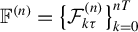 is the filtration constructed from the
$\sigma $
 -algebras
$\mathcal {F}^{(n)}_{k\tau }$
 denoting the information available to investors at time
$k\tau $
 and
$\mathbb {P}^{(n)}$
 represents the physical measure. The market consists of a risk-free and a risky asset whose price processes are denoted by
$B^{(n)} = \big \{ B^{(n)}_{k\tau } \big \}^{nT}_{k=0}$
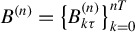 and
$S^{(n)} = \big \{ S^{(n)}_{k\tau } \big \}^{nT}_{k=0}$
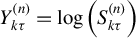
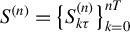 , respectively. We denote the logarithm of the risky asset price process by
$Y^{(n)} = \big \{ Y^{(n)}_{k\tau } \big \}^{nT}_{k=0}$
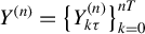 , so that
$Y^{(n)}_{k\tau } = \log \left (S^{(n)}_{k\tau }\right )$
 . The difference
$\Delta Y^{(n)}_{(k+1)\tau } = Y^{(n)}_{(k+1)\tau } - Y^{(n)}_{k\tau }$
 thus represents the risky asset’s log-return (henceforth return) from time
$k\tau $
 to
$(k+1)\tau $
 . The risk-free asset price at time
$k\tau $
 is assumed to be given by
$B^{(n)}_{k\tau } = e^{rk\tau }$
 , where r represents the constant continuously compounded risk-free rate. We further assume that the risky asset’s returns have the following n-augmented dynamics under measure
$\mathbb {P}^{(n)}$
 :


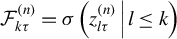
Here, we set
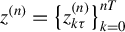
$\mathcal {F}^{(n)}_{k\tau } = \sigma \left (z^{(n)}_{l\tau } \, \middle | \, l \leq k \right )$
 , so that
$\mathbb {F}^{(n)}$
 is the natural filtration generated by the innovation process
$z^{(n)}=\big \{z^{(n)}_{k\tau } \big \}^{nT}_{k=0}$
 . We assume that
$z^{(n)}_{(k+1)\tau }$
 is a random variable following a generic distribution
$\mathcal {D}$
 with mean zero and variance
$h^{(n)}_{k\tau }$
 conditionally on
$\mathcal {F}_{k\tau }^{(n)}$
 and under measure
$\mathbb {P}^{(n)}$
 . The function
$F^{\mathcal {D}}$
 in Equation (1) represents the conditional mean excess return or equity risk premium. It is specified to depend on the conditional variance
$h^{(n)}_{k\tau }$
 and an equity risk premium parameter, denoted by
$\lambda (\tau )$
 , which varies with the discretization step
$\tau $
 .
The conditional variance
$h^{(n)}_{k\tau }$
 is decomposed into two components,
$s^{(n)}_{k\tau }$
 and
$q^{(n)}_{k\tau }$
 , following GARCH(1,1) dynamics given by Equations (3) and (4), respectively, where
$\Delta s^{(n)}_{(k+1)\tau } = s^{(n)}_{(k+1)\tau } - s^{(n)}_{k\tau }$
 and
$\Delta q^{(n)}_{(k+1)\tau } = q^{(n)}_{(k+1)\tau } - q^{(n)}_{k\tau }$
 . These dynamics rely on parameters that are dependent on the discretization step
$\tau $
 :
$\boldsymbol {\phi }(\tau ) = \big [\,\,\phi _{s}(\tau ) \quad \phi _{q}(\tau )\,\,\big ]^\top $
 is the vector of persistence parameters for
$s^{(n)}_{k\tau }$
 and
$q^{(n)}_{k\tau }$
 , respectively, satisfying
$0<\phi _s(\tau )<\phi _q(\tau )<1$
 for any
$\tau>0$
 ,
$\boldsymbol {\alpha }(\tau ) = \big [\,\,\alpha _{s}(\tau ) \quad \alpha _{q}(\tau )\,\,\big ]^\top $
 is the vector of nonnegative ARCH parameters associated with these components,
$\boldsymbol {\gamma }(\tau ) = \big [\,\,\gamma _{s}(\tau ) \quad \gamma _{q}(\tau )\,\,\big ]^\top $
 is the vector of leverage parameters, and
$\sigma ^2(\tau )>0$
 represents the unconditional mean of
$q^{(n)}_{k\tau }$
 , as well as of
$h^{(n)}_{k\tau }$
 .Footnote
7
The function
$G^{\mathcal {D}}$
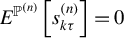
 is the GARCH variance driving noise function—a function of the return innovation process, the overall conditional variance, and the component-specific leverage parameter. We assume that

for
$u \in \{s,q\}$
 , so that
${E}^{\mathbb {P}^{(n)}}\left [s^{(n)}_{k\tau } \right ] = 0$
 and
${E}^{\mathbb {P}^{(n)}}\left [h^{(n)}_{k\tau } \right ] = {E}^{\mathbb {P}^{(n)}}\left [q^{(n)}_{k\tau } \right ] = \sigma ^2(\tau )$
 .
The modeling framework of Equations (1)–(4) generalizes the component GARCH model of Engle and Lee (Reference Engle and Lee1999). Their specification is nested as a special case by setting
$\tau =1$
 , adopting Gaussian-distributed innovations, and specifying particular functional forms for
$F^{\mathcal {D}}$
 and
$G^{\mathcal {D}}$
 . Following the terminology of Engle and Lee (Reference Engle and Lee1999), the decomposition
$h^{(n)}_{k\tau } = s^{(n)}_{k\tau } + q^{(n)}_{k\tau }$
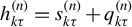 admits a natural interpretation in terms of short- and long-run variance components. In particular, the factor
$s^{(n)}_{k\tau }$
 represents the short-run component because it has zero unconditional mean and lower persistence than
$q^{(n)}_{k\tau }$
 , as implied by the restriction
$\phi _s(\tau )<\phi _q(\tau )$
 . It therefore captures relatively fast-moving transitory fluctuations in conditional variance. In contrast,
$q^{(n)}_{k\tau }$
 is interpreted as the long-run component because it has higher persistence and fluctuates around the long-run variance level
$\sigma ^2(\tau )$
 . This two-component structure is better able to capture the well-documented slow decay of the autocorrelation function of squared returns than a single-factor GARCH specification.
Remark 1. The one-component version of the above model is obtained by taking
$\phi _q(\tau ) = \alpha _{q}(\tau ) = 0$
 , so that the long-run variance component is constant, that is,
$q^{(n)}_{k\tau } = \sigma ^2(\tau )$
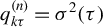 . Equation (3) can therefore be rewritten in terms of the conditional variance as

where
$\phi (\tau ), \alpha (\tau )$
 , and
$\gamma (\tau )$
 are the parameters of the conditional variance process.
2.1 Affine Assumptions
To establish an affine setting for the GARCH component modeling framework of Equations (1)–(4), we introduce the following assumption.
Assumption 1. For any real w and
$\boldsymbol {v} = \left [ \,\, v_1 \quad v_2 \,\, \right ]^{\top }$
 , the one-step
$\mathcal {F}^{(n)}_{k\tau }$
 -conditional joint cgf of
$\Delta Y^{(n)}_{(k+1)\tau }$
 ,
$ \Delta s^{(n)}_{(k+1)\tau }$
 , and
$ \Delta q^{(n)}_{(k+1)\tau }$
 is affine in the state variables with the following representation under measure
$\mathbb {P}^{(n)}$
 :

The coefficients
$\mathcal {A}^{\mathcal {D}}\left (w, \boldsymbol {v}; \tau \right )$
 and
$\mathcal {B}^{\mathcal {D}}_u\left (w, \boldsymbol {v}; \tau \right )$
 depend on the discretization step
$\tau $
 and are real-valued functions that satisfy
$\mathcal {A}^{\mathcal {D}}\left (0, \mathbf {0}; \tau \right ) = \mathcal {B}^{\mathcal {D}}_u\left (0, \mathbf {0}; \tau \right )= 0$
 for
$u \in \{s,q\}$
 .
Assumption 1 will be satisfied in the context of Equations (1)–(4) if and only if the following two conditions are met:
-
1. The function $F^{\mathcal {D}}$
 is affine in
$s^{(n)}_{k\tau }$
and
$ q^{(n)}_{k\tau }$
conditionally on
$\mathcal {F}^{(n)}_{k\tau }$
.
-
2. The joint cgf of $z^{(n)}_{(k+1)\tau }$
and
$G^{\mathcal {D}}$
is affine in
$s^{(n)}_{k\tau }$
and
$ q^{(n)}_{k\tau }$
conditionally on
$\mathcal {F}^{(n)}_{k\tau }$
.


While the first condition can be easily imposed when specifying the mean return dynamics, the second property can only be satisfied within two special classes of GARCH component processes, namely, the Gaussian and inverse Gaussian classes which will be introduced in Section 2.2.
Furthermore, the valuation of derivatives requires the specification of a martingale measure, which is not unique under our modeling assumptions. To preserve the affine property inherent in Assumption 1 under the risk-neutral measure, we introduce an n-augmented exponential affine pricing kernel in
$\Delta Y^{(n)}_{(k+1)\tau }$
 and the conditional variance components
$\Delta s^{(n)}_{(k+1)\tau }$
 and
$\Delta q^{(n)}_{(k+1)\tau }$
 .
Assumption 2. The risk-neutral probability measure denoted by
$\mathbb {Q}^{(n)}$
 is defined via the Radon–Nikodym derivative

where
$\theta (\tau )$
 and
$\boldsymbol {\xi }(\tau ) = \big [\,\, \xi _s(\tau ) \quad \xi _q(\tau ) \,\,\big ]^{\top }$
 represent the equity and variance component risk preference parameters, respectively; these parameters are also known as the market prices of risk in the literature. A nonzero value of the variance component risk preference parameter leads to a non-monotonic pricing kernel. We assume that these preference parameters satisfy the following system of equations:


Equations (8) and (9) ensure that the discounted asset price is a martingale under
$\mathbb {Q}^{(n)}$
 and are referred to as the martingale (or no-arbitrage) constraints. They follow directly from the martingale restriction,

and the affine form of the cgf provided in Assumption 1. These equations do not by themselves fully identify the pricing kernel parameters; solving them typically yields a relationship between the risk preference parameters, and in particular allows one to express
$\theta (\tau )$
 as a function of
$\boldsymbol {\xi }(\tau )$
 . The variance risk preference parameters
$\boldsymbol {\xi }(\tau )$
 are therefore not restricted by the martingale constraints and are left to be estimated from option prices, giving the pricing kernel the flexibility needed to better fit the option cross section. This is consistent with the variance-dependent pricing kernel approach of Christoffersen et al. (Reference Christoffersen, Heston and Jacobs2013) and contrasts with the remaining model parameters, which can be identified using return data.Footnote
8
2.2 Classes of Affine GARCH Models
This section presents two classes of affine GARCH component models. They are obtained as a special case of the general modeling framework introduced in Equations (1)–(4) by specifying the conditional distribution of the GARCH innovations
$\mathcal {D}$
 along with functions
$F^{\mathcal {D}}$
 and
$G^{\mathcal {D}}$
 . In addition, we prove a limiting relationship between these two classes of models.
2.2.1 The Gaussian GARCH Component Model
The Heston–Nandi GARCH component model, denoted by HN(C) in this article, was introduced by Christoffersen et al. (Reference Christoffersen, Jacobs, Ornthanalai and Wang2008) to generalize the one-component model proposed by Heston and Nandi (Reference Heston and Nandi2000). It is constructed based on a conditionally Gaussian assumption for the return innovation, that is,
$\mathcal {D} = \mathcal {N}$
 . More specifically, we assume that

where
$\epsilon ^{(n)}_{(k+1)\tau }$
 follows a standard Gaussian distribution, so that
$z^{(n)}_{(k+1)\tau }$
 is conditionally normally distributed with mean zero and variance
$h^{(n)}_{k\tau }$
 . The functions
${F}^{\mathcal {N}}$
 and
${G}^{\mathcal {N}}$
 are given by


for
$u \in \{s,q\}$
 , respectively. Following Augustyniak et al. (Reference Augustyniak, Badescu and Bégin2023), we show in Appendix A.1 that the n-augmented version of the HN(C) model belongs to the affine family introduced in Assumption 1. Moreover, as demonstrated in Appendix A.2.3, solving the martingale constraints (8) and (9) yields the following relationship between the risk preference parameters (see Equation (A.17)):

2.2.2 The Inverse Gaussian GARCH Component Model
The inverse Gaussian GARCH component model, denoted by IG(C) henceforth, was introduced by Babaoğlu et al. (Reference Babaoğlu, Christoffersen, Heston and Jacobs2018). It is an extension of the affine one-component GARCH model driven by inverse Gaussian innovations proposed by Christoffersen et al. (Reference Christoffersen, Heston and Jacobs2006). We denote the inverse Gaussian distribution by
$\mathcal {IG}$
 , and we define

where
$\epsilon ^{(n)}_{(k+1)\tau }$
 has a single parameter inverse Gaussian distribution with conditional mean and variance equal to
$h^{(n)}_{k\tau }/\eta ^2$
 . It follows that
$z^{(n)}_{(k+1)\tau }$
 has a shifted inverse Gaussian distribution with mean zero and variance
$h^{(n)}_{k\tau }$
 conditionally on
$\mathcal {F}^{(n)}_{k\tau }$
 . The skewness of the distribution of
$\epsilon ^{(n)}_{(k+1)\tau }$
 is given by
${3 |\eta |}\,\Big / \!{\sqrt {h^{(n)}_{k\tau }}}$
 , so that
$\eta $
 is usually called the skewness parameter. In practice,
$\eta $
 is negative, so that although
$\epsilon ^{(n)}_{(k+1)\tau }$
 is a positive random variable, the term
$z^{(n)}_{(k+1)\tau }$
 can generate both positive and negative returns (see Christoffersen et al., Reference Christoffersen, Heston and Jacobs2006, for more details on the inverse Gaussian models). The IG(C) model relies on the following specifications for
${F}^{\mathcal {IG}}$
 and
${G}^{\mathcal {IG}}$
 Footnote
9
:


We again show in Appendix A.1 that the n-augmented version of the IG(C) model belongs to the affine class of Assumption 1. Moreover, Section SM.D.3 of the Supplementary Material establishes that the martingale constraints (8) and (9) result in the following relationship:

2.2.3 Relationship between the Gaussian and Inverse Gaussian GARCH Models
Proposition 1 shows that the HN(C) model can be obtained as a limiting case of the IG(C) model by letting the skewness parameter
$\eta $
 go to zero under specific relationships between the parameters of the two models. The same result holds for one-component versions of these models.Footnote
10
Proposition 1. For any fixed
$k =0,\ldots ,nT-1$
 , the
$\mathcal {F}^{(n)}_{k\tau }$
 -conditional joint cgf of
$\Delta Y^{(n)}_{(k+1)\tau }$
 ,
$ \Delta s^{(n)}_{(k+1)\tau }$
 , and
$ \Delta q^{(n)}_{(k+1)\tau }$
 in the IG(C) model converges to the corresponding joint cgf in the HN(C) model as
$\eta $
 approaches zero, if the following parametric relationships hold between the two classes of models:

The superscripts
$\mathcal {N}$
 and
$\mathcal {IG}$
 on a parameter signify that the parameter corresponds to the HN(C) and IG(C) models, respectively.
Proof. See Section SM.D.1 of the Supplementary Material.
3 MAIN RESULTS ON THE WEAK LIMITS UNDER THE PHYSICAL AND RISK-NEUTRAL MEASURES
This section presents weak diffusion limits of the affine GARCH component models introduced in Section 2 for Gaussian and inverse Gaussian specifications, under both physical and risk-neutral measures.
We denote by
$\boldsymbol {X}^{(n)} = \big \{\boldsymbol {X}^{(n)}_{k\tau }\big \}^{nT}_{k=0}$
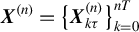 the discrete-time Markov process defined with respect to the filtration
$\mathbb {F}^{(n)}$
 representing the vector of our underlying processes of interest, that is, the vector
$\boldsymbol {X}^{(n)}_{k\tau }= \big [\,\,Y^{(n)}_{k\tau }\quad s^{(n)}_{k\tau }\quad q^{(n)}_{k\tau }\,\,\big ]^\top $
 satisfying the dynamics of Equations (1)–(4) under measure
${P}^{(n)}$
 .
The diffusion limits in this article are derived based on the weak convergence theorem of Markov processes to continuous-time diffusions (see Section SM.A of the Supplementary Material for details). First, we introduce the right-continuous with left limits (càdlàg) extension of the process
$\boldsymbol {X}^{(n)}$
 :

Assuming that
$\boldsymbol {X}^{(n)}_0$
 converges in distribution to a vector of random variables
$\boldsymbol {X}_0$
 as
$\tau $
 approaches zero, and provided that conditions (i)–(iii) of Theorem SM.1 in Section SM.A of the Supplementary Material are satisfied under a set of asymptotic scaling assumptions on the parameters, the process
$\{\boldsymbol {X}^{(n)}_t\}_{t \in [0,T]}$
 converges weakly to a three-dimensional diffusion process
$\{\boldsymbol {X}_t\}_{t \in [0,T]}$
 , where
$\boldsymbol {X}_t = \left [\,\,Y_t\quad s_t \quad q_t\,\,\right ]^\top $
 . Specifically, the weak limit process satisfies the time-homogeneous stochastic differential equation (SDE)

Here, the process
$\{\boldsymbol {W}_t\}_{t \in [0,T]}$
 is a three-dimensional standard Brownian motion on the filtered probability space
$\left (\Omega , \mathcal {F}, \mathbb {F}, \mathbb {P} \right )$
 , such that
$\boldsymbol {W}_t = \big [\,\,W_{1,t} \quad W_{2,t} \quad W_{3,t}\,\,\big ]^\top $
 and
$W_i = \{W_{i,t}\}_{t \in [0,T]}$
 are independent standard Brownian motions for
$i=1,2,3$
 .
We show that the weak limits of all affine discrete-time models considered in this study belong to the class of affine diffusion processes with coefficients having a specific representation as outlined below.Footnote
11
The drift coefficient
$ \boldsymbol {A}(\boldsymbol {X}_t)$
 is a three-dimensional vector satisfying

The diffusion coefficient
$\boldsymbol {\Sigma }( \boldsymbol {X}_t)$
 is a
$3 \times 3$
 lower triangular matrix which admits the decomposition

where
$\boldsymbol {\Gamma }$
 is a
$3 \times 3$
 lower triangular matrix of scalars and
$ \boldsymbol {V}\left (\boldsymbol {X}_t\right )$
 is a
$3 \times 3$
 diagonal matrix with the
$i^{\text {th}}$
 diagonal element having a square-root representation

with
$v_{0,i} \in \mathbb {R}$
 and
$\boldsymbol {v}_{1,i} \in \mathbb {R}^3$
 for any
$i = 1,2,3$
 . Equation (17) admits a unique (strong) solution
$\boldsymbol {X} = \{\boldsymbol {X}_t\}_{t \in \left [0,T\right ]}$
 under certain assumptions on the drift and diffusion coefficients (e.g., multidimensional Feller conditions). See Appendix A.2.2 for further details on these constraints in our specific setting.
The drift and diffusion coefficients in Equation (17) are model dependent, and we therefore augment them with the superscript
$\mathcal {D}$
 when referring to the weak limits of our Gaussian and inverse Gaussian specifications, that is,
$\mathcal {D}=\mathcal {N}$
 and
$\mathcal {D}=\mathcal {IG}$
 , respectively. These coefficients are determined based on the scaling assumptions imposed on the discrete-time model parameters as the time step
$\tau $
 approaches zero.
3.1 Asymptotic Scaling Assumptions Imposed on the Parameters
The asymptotic scaling assumptions imposed on the parameters to derive the weak diffusion limits of the affine GARCH component models introduced in Section 2 are summarized in Assumption 3.
Assumption 3. The equity risk premium and conditional variance parameters of the HN(C) and IG(C) models satisfy the following limiting constraints as the time step
$\tau $
 approaches zero.
-
A. Convergence Rates Governing First-Order Conditional Moments of $ \boldsymbol {X}^{(n)}$
: $$ \begin{align*} \lambda &= {\begin{cases} \begin{array}{ll} \lim\limits_{\tau \to 0} \tau^{-1} \lambda(\tau) & \text{for HN(C)}\\ \lim\limits_{\tau \to 0} \tau^{-1} \left(\lambda(\tau) + \dfrac{\sqrt{\tau}}{\eta} - \dfrac{\tau}{\eta} \right) & \text{for IG(C)}\\ \end{array}, \end{cases}} \quad \\ &\quad \sigma^2 = \lim\limits_{\tau \to 0} \sigma^2(\tau) , \qquad \boldsymbol{\kappa} = \lim\limits_{\tau \to 0} \tau^{-1}\left(\boldsymbol{1}- \boldsymbol{\phi}(\tau)\right). \end{align*} $$
-
B. Convergence Rates Governing Second-Order Conditional Moments of $\boldsymbol {X}^{(n)}$
: $$ \begin{align*} \boldsymbol{\alpha} = & \, \lim\limits_{\tau \to 0} \tau^{-\frac{1}{2}}\boldsymbol{\alpha}(\tau) , \qquad \boldsymbol{\gamma} = \lim\limits_{\tau \to 0} \boldsymbol{\gamma}(\tau). \end{align*} $$


All limits are assumed to be finite and in the following admissible ranges:
$\lambda \in \mathbb {R}$
 ,
$\sigma ^2> 0$
 ,
$\boldsymbol {\kappa }> \boldsymbol {0}$
 ,
$\boldsymbol {\alpha } \geq \boldsymbol {0}$
 , and
$\boldsymbol {\gamma } \in \mathbb {R}^2$
 .
First, notice that the first limiting constraint of Assumption 3A on the equity risk premium parameter
$\lambda (\tau )$
 is the only constraint that differs between the HN(C) and IG(C) specifications. Its role is to ensure that the risk premium term
$F^{\mathcal {D}}$
 in Equation (1) is of order
$O(\tau )$
 for both models, which guarantees the convergence of the first-order conditional moment of the return process. The remaining constraints of Assumption 3A govern the convergence of the first-order conditional moment of the variance components, while Assumption 3B ensures the convergence of all quantities from the conditional covariance matrix of
$\boldsymbol {X}^{(n)}$
 . Overall, Assumption 3 preserves the first- and second-order moment structure of the underlying discrete-time process as
$\tau $
 approaches zero, in the sense that the drift and covariance matrix of the diffusion limit process
$\boldsymbol {X}$
 exhibit the same functional representations as the corresponding conditional moments of
$\boldsymbol {X}^{(n)}$
 (see Appendix A.2.2 for more details).
We remark that it is straightforward to specify some functions
$\lambda (\tau )$
 ,
$\sigma ^2(\tau )$
 ,
$\boldsymbol {\phi }(\tau )$
 ,
$\boldsymbol {\alpha }(\tau )$
 , and
$\boldsymbol {\gamma }(\tau )$
 that satisfy the limiting constraints from Assumption 3. For example, we can set

The convergence rates proposed in Assumption 3 align with those used by Nelson (Reference Nelson1990) and Duan (Reference Duan1997) for establishing weak limits across a large plethora of non-affine GARCH models. In Section 4, we shall discuss the use of alternative convergence rates—including those previously adopted by the affine GARCH literature—for one-component Gaussian models. More specifically, we shall explain that the rates postulated in Assumption 3 lead to the most general diffusion dynamics and are the only ones capable of preserving the (conditional) moment structure of the underlying discrete-time affine process.
To conclude this section, we introduce a distributional invariant asymptotic constraint on the parameters governing the change of measure.
Assumption 4. The risk preference parameters in Equation (7) satisfy the following limiting relationship:

where
$\boldsymbol {\xi } \in \mathbb {R}^2$
 is finite.
Assumption 4 is required to establish the weak limits of the HN(C) and IG(C) models under the risk-neutral measure, or equivalently, the convergence of the Radon–Nikodym process.Footnote
12
As mentioned in Section 2.1, we can express
$\theta (\tau )$
 as a function of
$\boldsymbol {\xi }(\tau )$
 by solving Equations (8) and (9). Interestingly, the value of the equity risk preference parameter
$\theta (\tau )$
 is dependent on the discretization step and has a finite nonzero limit for both HN(C) and IG(C) models. For additional details, see Equations (A.17) and (A.18) in Appendix A.2.3 as well as Equations (SM.7) and (SM.8) in the Supplementary Material, respectively.
3.2 Weak Limits
The key ingredient for the computation of the drift and diffusion terms in Equation (17) within an affine setting is the asymptotic evaluation of the cross-cumulants of the underlying discrete-time process. Specifically, we can obtain these coefficients by computing partial derivatives of the conditional cgf of
$ \Delta \boldsymbol {X}^{(n)}_{k\tau }$
 evaluated at zero, and then taking their limits as
$\tau $
 approaches zero (see Appendix A.2.1 for more details). Although the dynamics of Equations (1)–(4) can also be used directly to compute the weak limits under the physical measure
$\mathbb {P}^{(n)}$
 , our approach does not require the a priori derivation of the risk-neutral dynamics of
$ \Delta \boldsymbol {X}^{(n)}_{k\tau }$
 for identifying the weak limits under
$\mathbb {Q}^{(n)}$
 .
3.2.1 Weak Limits under the Physical Measure
The diffusion limits of the HN(C) and IG(C) models under the physical measure are presented in Proposition 2.Footnote 13
Proposition 2. Assume that
$\big \{\boldsymbol {X}^{(n)}_{k\tau }\big \}^{nT}_{k=0}$
 follows the dynamics of Equations (1)–(4) under measure
$\mathbb {P}^{(n)}$
 , that Assumption 3 holds, and let
$h_t = s_t + q_t$
 . Then, as
$\tau $
 approaches zero, the process
$\{\boldsymbol {X}^{(n)}_t\}_{t \in [0,T]}$
 introduced in Equation (16) converges weakly to a three-dimensional diffusion process
$\{\boldsymbol {X}_t\}_{t \in [0,T]}$
 governed by the SDE of Equation (17),

with drift and diffusion coefficients given by:
-
(i) For the HN(C) model:
(22) $$ \begin{align} \boldsymbol{A}^{\mathcal{N}}\left(\boldsymbol{X}_t\right) = \begin{bmatrix} r + \lambda h_{t} \\ -\kappa_s s_t \\ \kappa_q\left(\sigma^2 - q_t \right) \\ \end{bmatrix},\qquad \boldsymbol{\Sigma}^{\mathcal{N}}\left(\boldsymbol{X}_t\right) = \begin{bmatrix} \sqrt{h_{t}} & 0 & 0 \\ - 2\alpha_s\gamma_s \sqrt{h_{t}} & \sqrt{2}\alpha_s & 0 \\ - 2\alpha_q\gamma_q \sqrt{h_{t}} & \sqrt{2}\alpha_q & 0 \\ \end{bmatrix}. \end{align} $$
-
(ii) For the IG(C) model:
(23) $$ \begin{align} \!\!\!\boldsymbol{A}^{\mathcal{IG}}\left(\boldsymbol{X}_t\right) = \!\begin{bmatrix}\! r + \lambda h_{t} \\ -\kappa_s s_t \\ \kappa_q\left(\sigma^2 - q_t\right) \\ \end{bmatrix},\quad\! \boldsymbol{\Sigma}^{\mathcal{IG}}\left(\boldsymbol{X}_t\right) = \begin{bmatrix}\!\! \sqrt{h_{t}} & 0 & 0 \\ \dfrac{\alpha_s\left(\gamma_s - \eta^4\right)}{\eta} \sqrt{h_{t}} & \sqrt{2}\eta^4\alpha_s & 0 \\ \dfrac{\alpha_q\left(\gamma_q - \eta^4\right)}{\eta} \sqrt{h_{t}} & \sqrt{2}\eta^4\alpha_q & 0 \\ \!\end{bmatrix}. \end{align} $$


The SDEs derived in Proposition 2 as the weak limits of the HN(C) and IG(C) models do not, in general, define SV models whose variance process can be guaranteed to remain nonnegative along all sample paths. This is due to the constant loading coefficient of the second Brownian motion in the limiting dynamics of the component factors
$s_t$
 and
$q_t$
 , which implies that these components cannot in general be constrained to be nonnegative with probability one. In particular, Appendix A.2.2 shows that the multidimensional Feller-type sufficient conditions of Duffie and Kan (Reference Duffie and Kan1996) are generally not fully satisfied by the diffusion limits in Proposition 2. However, this issue is not specific to the limiting dynamics and is also present in the underlying discrete-time component GARCH models (see, e.g., Majewski et al., Reference Majewski, Bormetti and Corsi2015; Oh and Park, Reference Oh and Park2023). Indeed, in these models, the short-run variance component can take negative values. In applications, however, the long-run component typically compensates for such movements so that the aggregate conditional variance remains positive along the realized path. The weak limiting result in Proposition 2 should therefore be interpreted as a local approximation on the domain where
$h_t>0$
 .
Moreover, both diffusion limits fit the continuous-time affine framework of Equations (18)–(20). For example, in the HN(C) case, the coefficients
$\boldsymbol {A}_0$
 and
$\boldsymbol {A}_1$
 from the drift term are given by

while the matrices
$\boldsymbol {\Gamma }$
 and
$\boldsymbol {V}\left (\boldsymbol {X}_t\right )$
 from the diffusion term decomposition are given by

with
$v_{0,1} = 0$
 and
$ \boldsymbol {v}_{1,1} = \big [\,\,0\quad 1\quad 1\,\,\big ]^\top $
 ,
$v_{0,j} = 1$
 and
$ \boldsymbol {v}_{1,j} = \big [\,\,0\quad 0\quad 0\,\,\big ]^\top $
 for
$j=2,3$
 , so that
$V_1\left (\boldsymbol {X}_t\right ) = \sqrt {h_t}$
 ,
$V_2\left (\boldsymbol {X}_t\right ) = V_3\left (\boldsymbol {X}_t\right ) = 1$
 . The drift and diffusion coefficients for the IG(C) limit have a similar structure.
In addition, both diffusion limits correspond to three-dimensional degenerate SV models.Footnote
14
Although the limiting SDE is written in the generic form of Equation (17) with a three-dimensional Brownian motion, the diffusion matrices
$\boldsymbol {\Sigma }^{\mathcal N}(\boldsymbol {X}_t)$
 and
$\boldsymbol {\Sigma }^{\mathcal {IG}}(\boldsymbol {X}_t)$
 are singular of rank two because their third column is identically zero. Hence, the third Brownian motion in the generic representation is redundant, and the limiting dynamics admit an equivalent formulation in terms of two independent Brownian motions only. However, this rank deficiency does not imply that one of the state equations becomes deterministic. The short- and long-run variance components are mean-reverting stochastic processes driven by two independent Brownian motions, one of which also drives the return process. The presence of a second Brownian motion in each variance component, and thus in the overall variance
$h_t$
 , comes in contrast with previous findings on the weak limits of one-component affine Gaussian GARCH models. These contrasting results can be explained by the use of different sets of asymptotic scaling assumptions on the model parameters and will be further analyzed in Section 4.
Interestingly, the HN(C) diffusion limit in Equation (22) coincides with that of the IG(C) model in Equation (23) if and only if the following relationships hold:

The relationships of Equation (24) are similar to those that ensure the convergence of the IG(C) model to the HN(C) model as
$\eta $
 approaches zero in Proposition 1. Indeed, under the parametric scaling specifications of Equation (21), the relationships in Equation (15) are analogous to those of Equation (24).
3.2.2 Weak Limits under the Risk-Neutral Measure
Proposition 3 establishes the diffusion limits of the HN(C) and IG(C) models under the risk-neutral measure.
Proposition 3. Assume that
$\big \{\boldsymbol {X}^{(n)}_{k\tau }\big \}^{nT}_{k=0}$
 follows the dynamics of Equations (1)–(4) under measure
$\mathbb {P}^{(n)}$
 , and that the risk-neutral probability measure
$\mathbb {Q}^{(n)}$
 is defined via the Radon–Nikodym derivative given in Assumption 2. Moreover, suppose that Assumptions 3 and 4 hold, and let
$h_t=s_t+q_t$
 . Then, as
$\tau $
 approaches zero, the process
$\{\boldsymbol {X}^{(n)}_t\}_{t \in [0,T]}$
 converges weakly to a three-dimensional diffusion process
$\{\boldsymbol {X}_t\}_{t \in [0,T]}$
 governed by the following SDE:

Here,
$\{\tilde {\boldsymbol {W}}_t\}_{t \in [0,T]}$
 is a three-dimensional standard Brownian motion under the risk-neutral measure, the diffusion matrix satisfies
$\tilde {\boldsymbol {\Sigma }}^{\mathcal {D}}( \boldsymbol {X}_t) = \boldsymbol {\Sigma }^{\mathcal {D}}( \boldsymbol {X}_t) $
 , where
$\boldsymbol {\Sigma }^{\mathcal {D}}( \boldsymbol {X}_t)$
 is obtained from Proposition 2, and the drift term is given by:
-
(i) For the HN(C) model:
(26) $$ \begin{align} \tilde{\boldsymbol{A}}^{\mathcal{N}}(\boldsymbol{X}_t) = \begin{bmatrix} r -\dfrac{1}{2}h_t \\[3pt] -\kappa_s s_t + 2 \alpha_s\gamma_s\left(\lambda+\dfrac{1}{2}\right)h_t + 2\alpha_s \boldsymbol{\alpha}^\top \boldsymbol{\xi} \\[3pt] \kappa_q\left(\sigma^{2} - q_t \right) + 2 \alpha_q\gamma_q\left(\lambda+\dfrac{1}{2}\right)h_t + 2\alpha_q \boldsymbol{\alpha}^\top \boldsymbol{\xi} \\ \end{bmatrix}. \end{align} $$
-
(ii) For the IG(C) model:
(27) $$ \begin{align} \tilde{\boldsymbol{A}}^{\mathcal{IG}}(\boldsymbol{X}_t) = \begin{bmatrix} r -\dfrac{1}{2}h_t \\[4pt] -\kappa_s s_t - \dfrac{\alpha_s\left(\gamma_s - \eta^4\right)}{\eta}\left(\lambda +\dfrac{1}{2}\right)h_t + 2\eta^8\alpha_s \boldsymbol{\alpha}^\top \boldsymbol{\xi} \\[4pt] \kappa_q\left(\sigma^{2} - q_t\right) - \dfrac{\alpha_q\left(\gamma_q - \eta^4\right)}{\eta}\left(\lambda +\dfrac{1}{2}\right)h_t + 2\eta^8\alpha_q \boldsymbol{\alpha}^\top \boldsymbol{\xi} \\ \end{bmatrix}. \end{align} $$


The drift coefficients of Equations (26) and (27) satisfy the general form of Equation (18), while the diffusion matrices remain unchanged after the change of measure. Consequently, the affine property of our weak limit process is preserved under the risk-neutral measure
$\mathbb {Q}$
 implied by the exponential affine pricing kernel of Assumption 2. Although the diffusion limit derived in Proposition 3 belongs to the affine class, it differs from the continuous-time option pricing models that are typically used in practice, such as the one in Christoffersen et al. (Reference Christoffersen, Heston and Jacobs2009) which consists of a two-factor Heston model with uncorrelated volatility components.
Furthermore, we note that the physical and risk-neutral dynamics of Propositions 2 and 3 are consistent with Girsanov’s principle. Specifically, we can recover the risk-neutral drift dynamics of Equations (26) and (27) by applying the standard change of measure provided by Girsanov’s theorem to the physical dynamics implied by Equations (22) and (23), respectively, for two particular choices of market prices of risk associated with the Brownian motions governing the variance component dynamics. Indeed, we can define the Radon–Nikodym derivative with respect to the two independent Brownian motions
$\{W_{1,t}\}_{t \in [0,T]}$
 and
$\{W_{2,t}\}_{t \in [0,T]}$
 from Proposition 2 via

which yields the risk-neutral dynamics of Proposition 3 if

This result can be easily verified for each model by defining two independent standard Brownian motions under
${Q}$
 ,
$\{\tilde {W}_{1,t}\}_{t \in [0,T]}$
 and
$\{\tilde {W}_{2,t}\}_{t \in [0,T]}$
 , with dynamics given by
$d\tilde {W}_{i,t} = d W_{i,t} + \nu _{i,t} \, dt$
 for
$i=1,2$
 . Thus, it comes as no surprise that, similarly to the physical measure case, the resulting risk-neutral diffusion limits of Equations (26) and (27) are identical if and only if the relationships of Equation (24) hold.
To conclude this section, we derive the cf of the risk-neutral diffusion limit obtained in Proposition 3. Such a function is typically required for the valuation of European-style derivatives in continuous time. Proposition 4 provides the
$\mathcal {F}_t$
 -conditional risk-neutral cf of
$\boldsymbol {X}_T$
 associated with the HN(C) limit. The corresponding cf in the IG(C) case can be obtained in a similar way by using the parametric relationships of Equation (24).
Proposition 4. Assume that the three-dimensional diffusion process
$\{\boldsymbol {X}_t\}_{t \in [0,T]}$
 with
$\boldsymbol {X}_t = \left [\,\,Y_t\quad s_t \quad q_t\,\,\right ]^\top $
 satisfies the SDE of Equation (25) with drift
$\tilde {\boldsymbol {A}}^{\mathcal {N}}( \boldsymbol {X}_t)$
 given in Equation (26) and diffusion matrix
$\tilde {\boldsymbol {\Sigma }}^{\mathcal {N}}( \boldsymbol {X}_t) = \boldsymbol {\Sigma }^{\mathcal {N}}( \boldsymbol {X}_t) $
 given in Proposition 2. Then, for any
$\boldsymbol {u} \in \mathbb {R}^3$
 , the
$\mathcal {F}_t$
 -conditional cf of
$\boldsymbol {X}_T$
 is

Here,
$\Phi (\boldsymbol {u}; T-t)$
 and
$ \boldsymbol {\Psi }(\boldsymbol {u}; T-t) = \left [ \, \, \Psi _1\left (\boldsymbol {u}; T-t \right ) \!\quad \Psi _2 \left (\boldsymbol {u}; T-t \right ) \!\quad \Psi _3\left (\boldsymbol {u}; T-t \right )\right ]^{\top }$
 are complex-valued functions satisfying the following system of ordinary differential equations (ODEs):

subject to the boundary constraints
$\Phi (\boldsymbol {u}; 0) = 0$
 and
$\boldsymbol {\Psi }\left (\boldsymbol {u}; 0\right ) = \mathrm {i} \boldsymbol {u}$
 .
Proof. See Section SM.B of the Supplementary Material.
We remark that although the second ODE can be solved explicitly (i.e.,
$\Psi _1(\boldsymbol {u};t) = \mathrm {i} u_1$
 ), the remaining system of quadratic ODEs for the coefficients
$\Psi _2(\boldsymbol {u};t)$
 and
$\Psi _3(\boldsymbol {u};t)$
 does not generally admit a closed-form solution, so one has to rely on numerical approximations to compute these coefficients (e.g., Runge–Kutta method). Nevertheless, explicit solutions can be obtained in specific cases, such as when there are no leverage effects (i.e.,
$\gamma _s=\gamma _q=0$
 ) or in the single-component case. In the latter instance, the system of ODEs can be solved in a similar fashion as that of the model of Heston (Reference Heston1993).
3.3 A Numerical Illustration of the Weak Limits
We now illustrate the impact of weak convergence limits of discrete-time affine GARCH models driven by both Gaussian and inverse Gaussian innovations on option prices. Specifically, we compute European call prices for the HN(C) and IG(C) models introduced in Section 2, risk-neutralized with the pricing kernel from Assumption 2, for different values of the number of discretization points per day n. The corresponding diffusion limit prices are obtained using the risk-neutral dynamics derived in Proposition 3.
European option prices can be expressed in semi-closed-form using Laplace or Fourier inversion methods for all discrete- and continuous-time affine models introduced in Sections 2 and 3. Indeed, the price at time
$t \in \mathcal {T}^{(1)}$
 of a K-strike European call option with maturity T is given by the integral representation (see, e.g., Augustyniak et al., Reference Augustyniak, Badescu and Bégin2023)

Here,
$\mathcal {C}^{\mathbb {Q}^{(n)}}_{Y_T^{(n)}} \big (z \,\big |\, \mathcal {F}_{t}^{(n)} \big )$
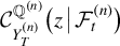 is the cgf of
$Y_T^{(n)}$
 conditional on
$\mathcal {F}_{t}^{(n)}$
 ,
$R>1$
 is a chosen constant, and the integration is performed along the vertical line
$\{z \in \mathbb {C} : \mathrm {Re}(z) = R\}$
 in the complex plane.Footnote
15
The corresponding continuous-time limit prices are computed based on a similar integral representation with the
$\mathcal {F}_t$
 -conditional cf of
$\boldsymbol {X}_T$
 under the risk-neutral measure
$\mathbb {Q}$
 derived in Proposition 4.
The parameters for the HN(C) model at the daily frequency (
$\tau =1$
 ) are taken from Augustyniak et al. (Reference Augustyniak, Badescu and Bégin2023), where they were estimated from S&P 500 returns and options data over 1996–2018 using a sequential maximum likelihood estimation method. Parameters for other time steps are obtained based on the scaling constraints in Equation (21), and we assume that the variance risk preference parameters are invariant to the discretization step, setting
$\boldsymbol {\xi }(\tau ) = \boldsymbol {\xi }$
 for all
$\tau $
 , which is consistent with the limiting behavior specified in Assumption 4. We consider two pricing kernels: a monotonic kernel with
$\boldsymbol {\xi }=\mathbf {0}$
 and a non-monotonic kernel with
$\boldsymbol {\xi }$
 estimated from market data following Augustyniak et al. (Reference Augustyniak, Badescu and Bégin2023). All parameter values for the HN(C) model with
$\tau =1$
 are reported in the note of Table 1. Moreover, the IG(C) parameters are obtained by setting
$\eta = -0.01$
 and applying the relationships from Proposition 1, so that the diffusion limits of both Gaussian and inverse Gaussian specifications coincide under the physical and risk-neutral measures. Unless stated otherwise, we assume an annualized risk-free rate of 2% (based on 252 trading days), an initial log-price
$Y_t^{(n)} = \log (100)$
 , and initial values of the short- and long-run variance components equal to their respective unconditional means.
Call option price convergence for the HN(C) and IG(C) models

Table 1 Long description
The table is divided into four panels: Panel A (H N (C) model, monotonic pricing kernel), Panel B (H N (C) model, non-monotonic pricing kernel), Panel C (I G (C) model, monotonic pricing kernel), and Panel D (I G (C) model, non-monotonic pricing kernel).
Each panel shares the same structure:
* Columns: Categorized by strike price K into In-the-money (K = 90), At-the-money (K = 100), and Out-of-the-money (K = 110). Each category is sub-divided into 3-month, 6-month, and 1-year maturities.
* Rows: Discretization points n starting at 1, then powers of 2 (2 super 2, 2 super 4, 2 super 6, 2 super 8), then 2 super 10, 2 super 12, 2 super 14, and finally the Limit.
Data Trends:
* In Panel A, prices for In-the-money 1-year maturity start at 14.709 at n = 1 and converge to a limit of 14.713. Out-of-the-money 3-month prices start at 0.407 and converge to 0.399.
* In Panel B, prices are generally higher than Panel A. In-the-money 1-year maturity starts at 15.794 and converges to 15.149. Out-of-the-money 3-month prices start at 0.666 and converge to 0.494.
* In Panel C, I G (C) monotonic prices show similar convergence to Panel A. In-the-money 1-year starts at 14.942 and limits at 14.713.
* In Panel D, I G (C) non-monotonic prices show the highest initial values, with In-the-money 1-year starting at 16.067 and converging to 15.149.
Across all panels, as n increases, the prices stabilize toward the Limit value, demonstrating numerical convergence.
Note: This table reports European call option prices for the two-component HN(C) and IG(C) models for various strike prices and times to maturity as a function of the number of discretization points per day n. The HN(C) model parameters are
$\lambda = 2.1190$
 ,
$\sigma ^2 = 1.2150 \times 10^{-4}$
 ,
$\phi _s = 0.87662$
 ,
$\alpha _s = 2.5842 \times 10^{-6}$
 ,
$\gamma _s = 3.6089 \times 10^{2}$
 ,
$\phi _q = 0.98939$
 ,
$\alpha _q = 1.8801 \times 10^{-6}$
 , and
$\gamma _q = 1.3387 \times 10^{2}$
 . The IG(C) model parameters are obtained using the relationships from Proposition 1 and assuming
$\eta =-0.01$
 . A monotonic pricing kernel is considered in Panels A and C and corresponds to
$\boldsymbol {\xi } = \big [\,\, 0 \quad 0 \,\,\big ]^{\top }$
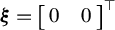 , while a non-monotonic pricing kernel is considered in Panels B and D and is obtained with
$\boldsymbol {\xi } = \big [\,\, 2.2798 \times 10^{3} \quad 3.7886 \times 10^{4} \,\,\big ]^{\top }$
 .
Table 1 reports the convergence of these European call option prices for three moneyness levels: in-the-money options (
$K=90$
 ), at-the-money options (
${K=100}$
 ), and out-of-the-money options (
$K=110$
 ), and three times to maturity:
$3$
 -month,
$6$
 -month, and
$1$
 -year. We notice that all discretized GARCH option prices converge smoothly to their corresponding diffusion limits. For any value of n, the HN(C) prices are consistently lower than the IG(C) counterparts, except for the shorter-term out-of-the-money options. As expected, when the constraints of Proposition 1 are satisfied, the weak limits of the HN(C) and IG(C) models are the same, and thus the limiting prices are identical, regardless of the shape of the pricing kernel (see, e.g., Panels A and C for monotonic pricing kernels, and Panels B and D for non-monotonic pricing kernels). The speed at which they converge to the limiting prices is however different—for the models exhibiting skewness, it generally takes more time for the prices to get closer to their limiting values.
The monotonic pricing kernel leads to limit prices that are less than those obtained with the non-monotonic pricing kernel, this being a by-product of the terms related to
$\boldsymbol {\xi }$
 in the drifts of Equations (26) and (27). Moreover, GARCH-based option prices computed at daily frequency (i.e.,
$\tau = 1$
 ) are closer to their corresponding diffusion limit prices for monotonic pricing kernels. For example, for the HN(C) model in Panel A, the smallest (largest) absolute difference for monotonic pricing kernels is $0.001 ($0.015). In contrast, the smallest (largest) absolute difference for the non-monotonic counterparts is $0.172 ($0.752) as shown in Panel B. This feature can be explained by the nonzero variance risk-preference parameter
$\boldsymbol {\xi }(\tau )$
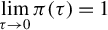
 assumed in the non-monotonic pricing kernels. Specifically, these kernels introduce a wedge between the physical and risk-neutral conditional variances for the discrete-time models, since
${V}^{\mathbb {Q}^{(n)}}[\Delta Y^{(n)}_{t+\tau } \mid \mathcal {F}_{t}^{(n)}]= \pi (\tau ) {V}^{\mathbb {P}^{(n)}}[\Delta Y^{(n)}_{t+\tau } \mid \mathcal {F}_{t}^{(n)}]$
 , for
$t\in \mathcal {T}^{(n)}$
 , with
$\pi (\tau )> 1$
 . Thus, when
$n = \tau =1$
 , the GARCH conditional risk-neutral variance is larger than the physical one; however, in the limit, the discrepancy between the two variances vanishes, as
$\lim \limits _{\tau \to 0} \pi (\tau ) = 1$
 .Footnote
16
Note that one way to reduce the gap between the GARCH prices and their diffusion limits under non-monotonic pricing kernels is to set
$\lim \limits _{\tau \to 0} \pi (\tau ) = \pi \neq 1$
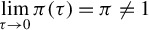 , which can be achieved using an alternative convergence rate for
$\boldsymbol {\xi }(\tau )$
 different from the one introduced in Assumption 4.Footnote
17
However, this modification would result in risk-neutral dynamics for the diffusion limits which can no longer be linked to the physical ones via Girsanov’s theorem. Finally, we remark that the differences between GARCH option prices computed at daily frequency and their diffusion limits generally increase for the IG(C) models due to the presence of
$\eta $
 , which is associated with a nonzero conditional skewness for the returns of the discrete-time models (see Panels C and D).
3.4 A Discussion of Possible Jump Limits
The weak limits derived in Propositions 2 and 3 for both the HN(C) and IG(C) models under the physical and risk-neutral measures are pure diffusion processes, driven by continuous Brownian motions. While diffusion-based SV models have long been the workhorse of continuous-time option pricing, there is compelling empirical and theoretical evidence that jumps play a significant role in modeling asset returns and option valuation (see, e.g., Bakshi et al., Reference Bakshi, Cao and Chen1997; Andersen et al., Reference Andersen, Benzoni and Lund2002; Eraker, Reference Eraker2004; Broadie et al., Reference Broadie, Chernov and Johannes2007; Andersen et al., Reference Andersen, Fusari and Todorov2015; Bollerslev and Todorov, Reference Bollerslev and Todorov2023). It is therefore natural to ask whether jump or jump-diffusion processes can arise as weak limits of the discrete-time affine GARCH models studied in this article, and under what conditions. The goal of this section is to address this question, first by reviewing the limited number of contributions in the literature that have tackled this problem, and then by discussing how a candidate jump limit may be constructed within our framework.
Despite the extensive literature on the continuous-time limits of GARCH processes, the derivation of jump or jump-diffusion limits from discrete-time GARCH models has received comparatively little attention. For example, Duan et al. (Reference Duan, Ritchken and Sun2006) extend the diffusion approximation framework of Nelson (Reference Nelson1990) and Duan (Reference Duan1997) to a class of GARCH-Jump models in which the standard Gaussian innovation is augmented with a Poisson random sum of Gaussian random variables. By allowing the jump intensity and the mean and variance of the Gaussian components to scale appropriately with the time step, they show that their GARCH-Jump approximating sequence converges to a bivariate jump-diffusion process in which both asset returns and variance exhibit correlated jump components alongside a diffusive element. Their limiting models nest the pure diffusion limits of Duan (Reference Duan1997), when the jump component is suppressed. Kallsen and Vesenmayer (Reference Kallsen and Vesenmayer2009) take a different approach and consider the weak limit of the standard GARCH(1,1) process toward a continuous-time GARCH (COGARCH) process driven by a general Lévy process, with volatility responding to its purely discontinuous quadratic variation. Their derivation relies on a random thinning mechanism and, in contrast with Nelson (Reference Nelson1990), the resulting limit features a single underlying source of randomness. However, both Duan et al. (Reference Duan, Ritchken and Sun2006) and Kallsen and Vesenmayer (Reference Kallsen and Vesenmayer2009) depart from the affine framework and their weak limits are also not in general affine processes.
At least to our knowledge, Christoffersen et al. (Reference Christoffersen, Heston and Jacobs2006) is the only study which presents a potential weak limit which includes jumps for an affine GARCH model driven by non-Gaussian innovations, more specifically for their inverse Gaussian GARCH process which is also nested by our general setting. Their analysis provides useful intuition for the type of limit one might expect. We note, however, that the specific assumptions used in their discussion differ from those that would be required for proving a functional weak convergence result in the sense of Nelson (Reference Nelson1990) for diffusions or Jacod and Shiryaev (Reference Jacod and Shiryaev2003) for general semimartingales, and it is worth clarifying these differences. First, their candidate limit is formulated in terms of a rescaled variance-rate process, and the conditions required to establish functional weak convergence are not formally verified. Second, the coefficient of the inverse innovation term in the conditional variance equation is set at
$0$
 , rather than as a function of the discretization step. As previously mentioned, for the discretized GARCH model to be internally consistent across sampling frequencies and to recover the unrestricted original daily model at
$\tau =1$
 , the parameters of the approximating sequence should depend on
$\tau $
 in a manner that is compatible with Assumption 3 or a jump-diffusion-limit analog. These observations motivate the alternative limiting constraints on the underlying model parameters that we advocate in this section, which are designed to satisfy both requirements simultaneously.
We now turn to the question of whether jump limits can arise from the affine models of Equations (1)–(4). In the Gaussian setting, under the model specifications and asymptotic scaling assumptions considered in this article, Condition (iii) of Theorem SM.1 in Section SM.A of the Supplementary Material is satisfied. This condition ensures that the increments of the approximating process do not generate jumps in the limit, and the resulting limiting processes therefore have continuous sample paths. Consequently, within the class of Gaussian affine GARCH approximating sequences and parameter scalings considered here, no jump component arises in the continuous-time limit.
The situation is richer in the inverse Gaussian setting. As shown in Proposition 2, under the scaling assumption of the IG innovations from Equation (1) and the asymptotic constraints from Assumption 3, Condition (iii) of Theorem SM.1 in Section SM.A of the Supplementary Material also holds true. Together with the first- and second-order conditional moment limits, this condition leads to a Brownian diffusion limit. To obtain a jump component in the returns limit, one must instead scale the innovation process so that the
$\mathcal {F}^{(n)}_{k\tau }$
 -conditional cgf of
$\Delta Y^{(n)}_{(k+1)\tau }$
 is linear in
$\tau $
 to leading order. This is the standard Lévy-type scaling, and it requires us to deviate from the modeling assumption made in Equation (1). Specifically, we remove the
$\sqrt {\tau }$
 scaling in front of the innovation process and allow the IG degrees of freedom parameter to be time-dependent so that the linearity property is satisfied, while preserving the affine structure. Under these specifications, the risky asset’s returns have the following dynamics under
$\mathbb {P}^{(n)}$
 :


Here, the innovation
$\epsilon ^{(n)}_{(k+1)\tau }$
 follows a single parameter inverse Gaussian distribution with mean and variance equal to
$\tau h^{(n)}_{k\tau }/\eta ^2$
 conditionally on
$\mathcal {F}^{(n)}_{k\tau }$
 , which satisfy the condition that both quantities scale at the same rate
$\mathcal {O}(\tau )$
 . Moreover, the
$\mathcal {F}^{(n)}_{k\tau }$
 -conditional cgf of
$\epsilon ^{(n)}_{(k+1)\tau }$
 admits the following linear representation under
$\mathbb {P}^{(n)}$
 :

It is easy to verify that under the cgf specification from Equation (31), Condition (iii) of Theorem SM.1 in Section SM.A of the Supplementary Material is no longer satisfied. To identify a plausible candidate jump limit for the above process, we consider asymptotic assumptions on the underlying parameters that differ from those used to derive the diffusion limits. Specifically, we impose the following scaling rates:

for some
$p>5/2$
 . We notice that while the convergence rates for the long-run variance parameter
$\sigma ^2(\tau )$
 and persistence
$\boldsymbol {\phi }(\tau )$
 are the same as in Assumption 3, those driving the variance of variance process are significantly different. The exponent p is not uniquely determined: any
$p>5/2$
 yields the same candidate limit below. Indeed, the product
$\boldsymbol {\alpha }(\tau )\odot \boldsymbol {\gamma }(\tau )$
 converges to a finite limit for every p, and, whenever the corresponding limit is nonzero, the
$\epsilon $
 channel contributes a jump to the variance dynamics, whereas the conditional variance per unit time of the centered
$1/\epsilon $
 channel is of order
$\mathcal {O}\left (\tau ^{2p-5}\right )$
 and therefore vanishes. Since only this product enters the limiting dynamics, the individual exponents are not separately identified. At the boundary
$p=5/2,$
 the centered
$1/\epsilon $
 channel instead contributes a non-degenerate Gaussian component, whereas for
$p<5/2,$
 its conditional variance per unit time diverges. Under these assumptions, the limiting conditional characteristics suggest that the (càdlàg) extension of the process
$\boldsymbol {X}^{(n)}_{k\tau }=\big [\,Y^{(n)}_{k\tau }\quad s^{(n)}_{k\tau }\quad q^{(n)}_{k\tau }\,\big ]^\top $
 that follows the dynamics from Equations (28) to (30) has the candidate limit
$\boldsymbol {X}_t=\big [\,Y_t\quad s_t\quad q_t\,\big ]^\top $
 , which satisfies the following SDEs:


Here,
$L_t$
 is a state-dependent pure-jump process of inverse Gaussian type whose jump measure has compensator
$h_{t-}\eta ^{-2}\nu _{\mathcal {IG}}(dx)\,dt$
 , where
$\nu _{\mathcal {IG}}$
 denotes the unit inverse Gaussian Lévy measure. A rigorous proof of the corresponding weak convergence result would follow the prescription of Theorem IX.3.39 from Jacod and Shiryaev (Reference Jacod and Shiryaev2003). However, since the focus of our article is on diffusion limits, we leave the rigorous treatment of this convergence result, including its numerical implementation and empirical analysis, for future research.
Several features of the candidate limiting dynamics in Equations (32)–(34) are noteworthy. First, similarly to the candidate limit discussed by Christoffersen et al. (Reference Christoffersen, Heston and Jacobs2006), all three state variables
$Y_t$
 ,
$s_t$
 , and
$q_t$
 are driven by the same jump process
$L_t$
 . However, this common source of randomness does not imply market completeness, because the continuum of possible jump-size risks need not be spanned by the traded risky asset. Second, the candidate limiting process is a pure-jump process with no diffusion component. Although pure-jump processes are theoretically tractable and have been used in the option pricing literature, they tend to be less flexible than jump-diffusion models for fitting implied volatility surfaces. A more flexible structure is already available within the same modeling framework at the boundary rate
$p=5/2$
 , for which the variance components acquire an additional Gaussian component and the candidate limit becomes a jump-diffusion; the returns, however, remain purely discontinuous under any of these scalings, since the innovation enters Equation (28) only through
$\epsilon ^{(n)}_{(k+1)\tau }$
 . A possible way to enrich the return dynamics is therefore to augment the return equation with an independent Gaussian diffusion component, similarly to the approach of Duan et al. (Reference Duan, Ritchken and Sun2006) for their jump-GARCH option pricing model. Such a modification, however, would require a separate analysis of the affine property and of the corresponding limiting and risk-neutral dynamics.
An affine alternative that could allow for a richer jump-diffusion limiting structure has been proposed in discrete time by Ornthanalai (Reference Ornthanalai2014), who introduces a class of Lévy GARCH models in which the returns are modeled with the sum of a Gaussian and a pure-jump Lévy component with time-homogeneous parameters that follow Heston and Nandi (Reference Heston and Nandi2000) dynamics, which is required for preserving the affine property. Because the variance dynamics are driven only by the Gaussian part, this specification can be viewed as a hybrid GARCH-SV model with heavy-tailed innovations. Using the same intuition as above, the resulting limit would be a jump-diffusion process for the returns driven by two independent sources of randomness—a Brownian motion and a Lévy process—and with no jumps in the time-homogeneous factors. Unlike in the jump-driven IG limiting case, this setting allows for more general pricing kernels which can incorporate equity, volatility, and jump risk aversion coefficients, yielding a more empirically appealing continuous-time model for option pricing. This is a natural direction for future research and some of the results derived in this article provide the key building block for such an extension.
4 REVISITING THE RELATIONSHIP BETWEEN DISCRETE AND CONTINUOUS-TIME AFFINE MODELS
This section relates the affine GARCH weak limit derived in Section 3 to the one obtained by Heston and Nandi (Reference Heston and Nandi2000). Specifically, we investigate the impact of using different parametric convergence rates on the resulting diffusion limit. We extend our analysis to include two new categories of GARCH models that feature SV, aiming to understand the connection between affine models in discrete and continuous time. Moreover, we explain why the asymptotic scaling assumptions postulated in Assumption 3 are the most natural ones to consider for relating GARCH models to diffusion processes through weak convergence.
For the sake of exposition, we focus our analysis in this section on the limiting behavior of one-component Gaussian models under the physical measure. To simplify the notation, we remove the distribution superscript
$\mathcal {N}$
 henceforth. In addition, the underlying discrete-time process
$\boldsymbol {X}^{(n)} = \big \{\boldsymbol {X}^{(n)}_{k\tau }\big \}^{nT}_{k=0}$
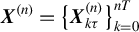 is now assumed to be two-dimensional with
$\boldsymbol {X}^{(n)}_{k\tau }= \big [\,\,Y^{(n)}_{k\tau }\quad h^{(n)}_{k\tau }\,\,\big ]^\top $
 , so that its weak limit
$\boldsymbol {X}_t = \big [\,\,Y_t\quad h_t \,\,\big ]^{\top }$
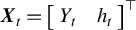 represents the solution of the SDE in Equation (17), where
$\{\boldsymbol {W}_t\}_{t \in [0,T]}$
 is now a two-dimensional standard Brownian motion,
$\boldsymbol {A}(\boldsymbol {X}_t)$
 is a two-dimensional vector of drift terms, and
$\boldsymbol {\Sigma }\left (\boldsymbol {X}_t\right )$
 is a
$2 \times 2$
 lower triangular matrix containing the diffusion terms; both
$\boldsymbol {A}(\boldsymbol {X}_t)$
 and
$\boldsymbol {\Sigma }\left ( \boldsymbol {X}_t\right )$
 adhere to the affine structure of Equations (18)–(20).
4.1 Revisiting the Heston and Nandi (Reference Heston and Nandi2000) Diffusion Limit
Following Remark 1, the discretized one-component affine Gaussian GARCH model of Heston and Nandi (Reference Heston and Nandi2000), denoted henceforth by HN, is obtained by setting
$\phi (\tau ) = \phi _s(\tau )$
 ,
$\alpha (\tau ) = \alpha _s(\tau )$
 ,
$\gamma (\tau ) = \gamma _s(\tau )$
 , and assuming
${\phi _q(\tau ) = \alpha _q(\tau ) = 0}$
 , so that
$q^{(n)}_{k\tau } = \sigma ^2(\tau )$
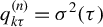 and
$s^{(n)}_{k\tau } = h^{(n)}_{k\tau }- \sigma ^2(\tau )$
 . Corollary 1 provides the diffusion limit of the HN model that is obtained as a special case of Proposition 2.
Corollary 1. Assume that
$\big \{\boldsymbol {X}^{(n)}_{k\tau }\big \}^{nT}_{k=0}$
 follows the dynamics of the discretized HN model under measure
$\mathbb {P}^{(n)}$
 . Further suppose that the limiting parameter scaling constraints in Assumption 3 hold. Then, as
$\tau $
 approaches zero, the process
$\{\boldsymbol {X}^{(n)}_t\}_{t \in [0,T]}$
 converges weakly to a two-dimensional diffusion process
$\{\boldsymbol {X}_t\}_{t \in [0,T]}$
 governed by the following SDEs:


Here,
$\{W_{1,t}\}_{t \in [0,T]}$
 and
$\{W_{2,t}\}_{t \in [0,T]}$
 are two independent standard Brownian motions on
$\left (\Omega , \mathcal {F}, \mathbb {F}, \mathbb {P} \right )$
 .
Proof. The diffusion limit of the HN model can be obtained directly from Equation (22) by assuming
$q_t = \sigma ^2$
 , so that
$dq_t = 0$
 and
$dh_t = d s_t$
 , and letting
$\kappa = \kappa _s$
 ,
$\alpha = \alpha _s$
 , and
$\gamma = \gamma _s$
 .
In contrast to the component case of Proposition 2, the HN limit presented in Corollary 1 is a non-degenerate diffusion process. The conditional variance dynamics of Equation (36) contain two sources of noise, which is a result commonly obtained when deriving diffusion limits in non-affine (one-component) GARCH settings under similar convergence rates for the underlying parameters (see, e.g., Nelson, Reference Nelson1990; Duan, Reference Duan1997). Note that Equation (36) can be reformulated using a single Brownian motion as follows:

Here,
$W^\prime _{2} = \{W^\prime _{2,t}\}_{t \in [0,T]}$
 is a Brownian motion that exhibits a stochastic correlation with the Brownian motion governing the return dynamics, such that
$d\langle W_{1}, W^\prime _{2} \rangle _t = -\dfrac {2\,\gamma \,\sqrt {h_t}}{\sqrt {2 + 4\,\gamma ^2\,h_t}}\, dt$
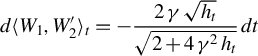 . This limit is also consistent with the result from Han et al. (Reference Han, Khrapov and Renault2020), who obtained a similar CIR-type limit for a discrete-time affine SV model under comparable asymptotic assumptions, with their scaling implied by the temporal aggregation property of the integrated volatility process.
It is important to highlight that the HN limit presented in Corollary 1 differs from the one derived by Heston and Nandi (Reference Heston and Nandi2000), which corresponds to a two-dimensional degenerate diffusion where returns and volatility dynamics are driven by the same Brownian motion. Specifically, the Heston and Nandi (Reference Heston and Nandi2000) diffusion limit comprises the same dynamics for the return process as in Equation (35), but involves a simpler SDE for the variance dynamics:

This diffusion limit corresponds to a special case of the model of Heston (Reference Heston1993) that is driven by perfectly (negatively) correlated Brownian motions with a volatility of volatility parameter equal to
$2 \alpha \gamma $
 . The disparity between our limit and that established by Heston and Nandi (Reference Heston and Nandi2000) can be explained by the fact that the latter limit was derived assuming different limiting constraints for the parameters
$\alpha (\tau )$
 and
$\gamma (\tau )$
 ; specifically, they usedFootnote
18

These constraints, in contrast to those in Assumption 3B, imply different scaling behaviors for
$\alpha (\tau )$
 and
$\alpha (\tau ) \, \gamma (\tau )$
 , with rates of
$\tau $
 and
$\tau ^{1/2}$
 , respectively. This discrepancy leads to an asymmetry in the loadings of the affine GARCH driving noise function as
$\tau $
 approaches zero, altering the limiting dynamics. To understand this, consider the expression representing the noise driving the conditional variance dynamics in the HN model as per Equation (5):

This equation involves linear and quadratic functions of the innovation that are multiplied by
$\alpha (\tau ) \, \gamma (\tau )$
 and
$\alpha (\tau )$
 , respectively. If
$\alpha (\tau )$
 scales faster to zero than
$\alpha (\tau ) \, \gamma (\tau )$
 , the linear noise component
$- 2\, \alpha (\tau )\,\gamma (\tau ) \, z^{(n)}_{(k+1)\tau }$
 dominates over the quadratic one, leading to an asymptotic setting where the return and variance dynamics are both driven by a linear function of the innovation
$z^{(n)}_{(k+1)\tau }$
 . This explains why the Heston and Nandi (Reference Heston and Nandi2000) diffusion limit contains a single Brownian motion driving both returns and variance dynamics, while our limit includes an additional Brownian motion that accounts for the quadratic noise component in Equation (40).
We remark that if there is no leverage effect in the HN model (i.e.,
$\gamma =0$
 ), the Heston and Nandi (Reference Heston and Nandi2000) diffusion limit exhibits a deterministic variance process, akin to the non-affine GARCH(1,1) weak limit derived by Corradi (Reference Corradi2000). In fact, the scaling assumption of
$\tau ^{-1}$
 for
$\alpha (\tau )$
 made by Heston and Nandi (Reference Heston and Nandi2000) aligns with that of Corradi (Reference Corradi2000), while our assumption of
$\tau ^{-1/2}$
 is in line with Nelson (Reference Nelson1990) and Duan (Reference Duan1997).
Furthermore, it can be shown that
$\alpha (\tau )$
 and
$\alpha (\tau )\, \gamma (\tau )$
 must scale at the rate
$\tau ^{1/2}$
 to preserve the second-order moment structure of the underlying affine GARCH dynamics in the limit (see Appendix A.2.2 for more details). For example, the conditional variance of variance function in the HN model is
${V}^{\mathbb {P}^{(n)}}[h^{(n)}_{t+\tau } \mid \mathcal {F}_{t}^{(n)}]=2\alpha ^2(\tau ) + 4\alpha ^2(\tau )\, \gamma ^2(\tau )h^{(n)}_t$
 , for
$t\in \mathcal {T}^{(n)}$
 . In our limit, the instantaneous variance of variance function implied by Equation (36) is
$2\alpha ^2 + 4\alpha ^2\gamma ^2 h_t$
 , while it is
$4\alpha ^2\gamma ^2 h_t$
 in the Heston and Nandi (Reference Heston and Nandi2000) limit. The absence of the term
$2\alpha ^2$
 in their limit is due to the asymmetric scaling behavior of
$\alpha (\tau ) \, \gamma (\tau )$
 and
$\alpha (\tau )$
 , as previously discussed. Another difference between the dynamics in Equations (36) and (38) is that the latter are driven by three free parameters instead of four.Footnote
19
4.2 Characterization of Weak Limits for a New Discrete-Time Affine GARCH Stochastic Volatility Model
The fact that different diffusion limits can be derived under distinct parametric convergence rates motivates us to study the diffusion processes that can be obtained as a limit of an affine discrete-time process. To this end, we consider a generalization of the HN model that was recently proposed by Heston et al. (Reference Heston, Jacobs and Kim2024a), and refer to it as the Heston–Nandi SV model, henceforth denoted by HNSV.
We introduce this model under a modified parametrization that fits the general discrete-time framework presented in Section 2. The discretized HNSV dynamics under the physical measure
$\mathbb {P}^{(n)}$
 are given by


Here,
$\left (\epsilon ^{(n)}_{(k+1)\tau }, \psi ^{(n)}_{(k+1)\tau }\right )$
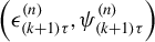 follows an
$\mathcal {F}^{(n)}_{k\tau }$
 -conditional bivariate standard Gaussian distribution with correlation coefficient
$\rho $
 . Apart from the parameter
$\rho $
 , this model shares the same parameters as the HN model, namely,
$\lambda (\tau )$
 ,
$\phi (\tau )$
 ,
$\sigma ^2(\tau )$
 ,
$\alpha (\tau )$
 , and
$\gamma (\tau )$
 , which are defined analogously as in Section 2. It can be interpreted as an HN process in which the innovation driving the variance dynamics is correlated with—but no longer the same as—the one driving returns. Clearly, the HN model is recovered as a special case when
$\rho =1$
 . Moreover, Section SM.D.4 of the Supplementary Material confirms that the HNSV model satisfies the affine property of Assumption 1. Consequently, this process is akin to a continuous-time SV model driven by two correlated Brownian motions and is thus a perfect candidate for studying the limiting relationship between affine models in discrete and continuous time.
To relate Equations (41) and (42) to the modeling framework introduced in Section 2, note that Equation (41) is identical to Equation (1) with
$F^{\mathcal {D}}\left (h^{(n)}_{k\tau }; \lambda (\tau ) \right ) = F^{\mathcal {N}}\left (h^{(n)}_{k\tau }; \lambda (\tau ) \right ) = \lambda (\tau ) \, h^{(n)}_{k\tau }$
 as in Equation (11). In addition, Equation (42) can be expressed in the form of Equation (5), that is,

where the function
$G^{\mathcal {D}}$
 is now expressed in terms of a new innovation,
$w^{(n)}_{(k+1)\tau } = \sqrt {h^{(n)}_{k\tau }} \, \psi ^{(n)}_{(k+1)\tau }$
 , as follows:

Although
$G^{\mathcal {D}}$
 is a function of a new innovation, its functional form is identical to the one we considered for the Gaussian class of affine GARCH models introduced in Section 2.
Throughout the remainder of this section, we assume that the parameters of the discretized HNSV model satisfy Assumption 3A. However, Assumption 3B is replaced by Assumption 5, which comprises all power-law convergence rates for
$\alpha (\tau )$
 and
$\gamma (\tau )$
 that result in a diffusion matrix with finite entries.
Assumption 5. The parameters
$\alpha (\tau )$
 and
$\gamma (\tau )$
 of the discretized HNSV model satisfy the following asymptotic relationships:

where
$\delta _1 \geq 0$
 and
$\delta _2 \geq - \delta _1$
 .
The asymptotic relationships that were postulated in Assumption 3B are the slowest convergence rates that can be considered for
$\alpha (\tau )$
 and
$\gamma (\tau )$
 , that is, they can be obtained by setting
$\delta _1=\delta _2 =0$
 in Assumption 5. The convergence rates employed by Heston and Nandi (Reference Heston and Nandi2000) and given in Equation (39) correspond to the case
$\delta _1=1/2$
 and
$\delta _2=-1/2$
 . Proposition 5 provides a characterization of the HNSV diffusion limits that can be obtained under all possible combinations of
$\delta _1$
 and
$\delta _2$
 .
Proposition 5. Assume that
$\big \{\boldsymbol {X}^{(n)}_{k\tau }\big \}^{nT}_{k=0}$
 follows the discretized HNSV dynamics from Equations (41) and (42) under measure
$\mathbb {P}^{(n)}$
 , and Assumptions 3A and 5 hold. Then, as
$\tau $
 approaches zero, the process
$\{\boldsymbol {X}^{(n)}_t\}_{t \in [0,T]}$
 converges weakly to a two-dimensional diffusion process
$\{\boldsymbol {X}_t\}_{t \in [0,T]}$
 governed by the following SDEs:

and

Here,
$\{W_{1,t}\}_{t \in [0,T]}$
 and
$\{W_{2,t}\}_{t \in [0,T]}$
 are two independent standard Brownian motions on
$\left (\Omega , \mathcal {F}, \mathbb {F}, \mathbb {P} \right )$
 .
Proof. See Section SM.D.4 of the Supplementary Material.
First, we observe that all weak limits derived in Proposition 5 belong to the class of affine diffusion processes. The diffusion limit with the most general variance dynamics emerges when both
$\delta _1$
 and
$\delta _2$
 are equal to zero, which corresponds to the setting of Assumption 3B. In this scenario,
$\alpha (\tau )$
 and
$\alpha (\tau )\,\gamma (\tau )$
 both scale at the rate
$\tau ^{1/2}$
 , which allows us to preserve the effects of the linear and quadratic components of the noise function asymptotically, as discussed in Section 4.1. The other three cases result in either the linear or quadratic noise components vanishing in the limit. This occurs when the scaling rates of
$\alpha (\tau )$
 or
$\alpha (\tau )\,\,\gamma (\tau )$
 exceed
$\tau ^{1/2}$
 . In particular, in the last case (i.e.,
$\delta _1> 0$
 and
$\delta _2> -\delta _1$
 ), the noise elements completely vanish, leading to a deterministic variance process—a structure that is not consistent with the underlying HNSV dynamics. In the third case (i.e.,
$\delta _1=0$
 and
$\delta _2>0$
 ), the variance dynamics follow an Ornstein–Uhlenbeck process that is uncorrelated with the return dynamics. Since the GARCH leverage effect parameter
$\gamma $
 does not appear in the limiting dynamics, this case fails to capture a fundamental characteristic in the structure of the HNSV model. The second case (i.e.,
$\delta _1>0$
 and
$\delta _2 = -\delta _1$
 ) leads to the classical Heston (Reference Heston1993) model where return and variance dynamics are driven by two correlated Brownian motions with a constant correlation coefficient.Footnote
20
This result can be viewed as a generalization of the Heston and Nandi (Reference Heston and Nandi2000) limit for the HN model since the latter is obtained as a special case by taking
$\rho =1$
 . However, the underlying parametric convergence rates lead to a diffusion process that does not have the same variance of variance structure as the HNSV model, similarly to our discussion for the HN model in Section 4.1.
The dynamics of the variance process obtained in Proposition 5 for the case
$\delta _1=\delta _2 =0$
 can be reformulated using a single Brownian motion as in Equation (37). However, the stochastic correlation between the Brownian motions
$W_{1}^{\vphantom {\prime }}$
 and
$W^\prime _{2}$
 has now a more flexible form as it is a function of the new parameter
$\rho $
 , that is,
$d\langle W_{1}^{\vphantom {\prime }}, W^\prime _{2} \rangle _t = -\rho \dfrac {2\,\gamma \,\sqrt {h_t}}{\sqrt {2 + 4\,\gamma ^2\,h_t}}\, dt$
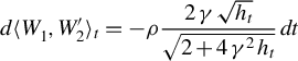 . We remark that nonzero
$\gamma $
 and
$\rho $
 are necessary to induce a leverage effect in both continuous- and discrete-time dynamics. This entails that simply having correlated innovations affecting return and variance dynamics is not enough for generating a leverage effect; the
$\gamma $
 parameter plays a critical role. Moreover, the instantaneous variance of variance function in this model is not directly proportional to
$h_t$
 as in the model of Heston (Reference Heston1993). Consequently, this diffusion limit has somewhat more complex variance dynamics compared to Heston’s (Reference Heston1993) model, and features five parameters instead of four. This additional flexibility may explain why Heston et al. (Reference Heston, Jacobs and Kim2024a) found that the HNSV model slightly outperformed Heston’s model in an empirical experiment.
4.3 Relating Continuous-Time Canonical Affine Stochastic Volatility Models to GARCH Processes
Section 4.2 showed that the affine SV model of Heston (Reference Heston1993), which assumes a constant correlation, cannot be obtained as a weak limit of a discrete-time affine model from the GARCH class without making specific asymptotic scaling assumptions on the parameters that alter the moment structure of the process as the time step approaches zero.Footnote 21
Ishida and Engle (Reference Ishida and Engle2002) introduce an SQGARCH model that converges weakly to Heston’s model using parametric scaling assumptions that are consistent with Nelson (Reference Nelson1990) and those in Assumption 3. However, there is a caveat—this SQGARCH model does not satisfy Assumption 1 and is therefore not affine. In other words, the canonical (one-factor) affine classes of models popularized in discrete and continuous time are not analogous to one another from the point of view of weak convergence.
More generally, Ishida and Engle (Reference Ishida and Engle2002) show that the CEV SV diffusion process (see, e.g., Jones, Reference Jones2003, and the references therein), which encompasses the models of Hull and White (Reference Hull and White1987) and Heston (Reference Heston1993), can be obtained as a weak limit of a GARCH class of processes, which they introduced as CEVGARCH. The variance dynamics of this process obey the general form of Equation (5) with a variance driving noise function given by

where
$p \geq 0$
 . The SQGARCH is obtained as a special case for
$p=1/2$
 . When
$p=1$
 , the variance dynamics correspond to the non-linear asymmetric GARCH of Engle and Ng (Reference Engle and Ng1993). This model has been proposed for option valuation by Duan (Reference Duan1995) and is now the standard non-affine GARCH model used in the option pricing literature.
Just as the HN model can be extended to HNSV, we consider here a generalization of the CEVGARCH model that allows the return and variance equations to be driven by different innovations. We refer to this generalization as the CEVSV model. Its discretized dynamics under the physical measure
$\mathbb {P}^{(n)}$
 are given by


Here,
$\left (\epsilon ^{(n)}_{(k+1)\tau }, \psi ^{(n)}_{(k+1)\tau }\right )$
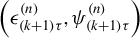 follows an
$\mathcal {F}^{(n)}_{k\tau }$
 -conditional bivariate standard Gaussian distribution with correlation coefficient
$\rho $
 . The CEVGARCH model of Ishida and Engle (Reference Ishida and Engle2002) is obtained as a special case of CEVSV by taking
$\rho =1$
 . Unlike the previous models considered, the CEVSV specification is generally non-affine. Section SM.D.5 of the Supplementary Material shows that it is non-affine for every
$p>0$
 . When
$p=0$
 , the model is affine only if
$\rho \gamma (\tau )=0$
 , apart from the trivial case
$\alpha (\tau )=0$
 . Proposition 6 provides a characterization of the CEVSV diffusion limits across all possible combinations of
$\delta _1$
 and
$\delta _2$
 in Assumption 5.
Proposition 6. Assume that
$\big \{\boldsymbol {X}^{(n)}_{k\tau }\big \}^{nT}_{k=0}$
 follows the dynamics of the discretized CEVSV dynamics from Equations (47) and (48) under measure
$\mathbb {P}^{(n)}$
 , and Assumptions 3A and 5 hold. Then, as
$\tau $
 approaches zero, the process
$\{\boldsymbol {X}^{(n)}_t\}_{t \in [0,T]}$
 converges weakly to a two-dimensional diffusion process
$\{\boldsymbol {X}_t\}_{t \in [0,T]}$
 governed by the following SDEs:

and

Here,
$\{W_{1,t}\}_{t \in [0,T]}$
 and
$\{W_{2,t}\}_{t \in [0,T]}$
 are two independent standard Brownian motions on
$\left (\Omega , \mathcal {F}, \mathbb {F}, \mathbb {P} \right )$
 .
Proof. See Section SM.D.5 of the Supplementary Material.
When
$\delta _1=\delta _2=0$
 , the diffusion limit of the CEVSV model corresponds to the CEV SV model studied by Jones (Reference Jones2003) and is no more general than that obtained for the CEVGARCH assuming
$\rho =1$
 . Indeed, we can express the variance dynamics as follows:

where
$\rho ^\prime = - 2\gamma \rho \, \Big / \left (\!\sqrt {2+4\gamma ^2}\right )$
 . This indicates that the parameters
$\gamma $
 and
$\rho $
 are not identifiable in the continuous-time dynamics, implying that the diffusion limit assuming
$\rho =1$
 can exhibit dynamics indistinguishable from those with a general
$\rho $
 . This is in contrast to the weak limit of the HNSV model, where all parameters are identifiable and which is not equivalent to its GARCH counterpart’s limit. Moreover, we note that nonzero
$\gamma $
 and
$\rho $
 are necessary to induce a leverage effect in both continuous- and discrete-time dynamics, similarly to the HNSV setting.
The weak limits of the CEVSV model belong to the class of affine diffusion processes for
$p=1/2$
 , and also for
$p=0$
 when the return–variance covariance vanishes (see Section SM.D.5 of the Supplementary Material for more details).Footnote
22
This indicates that the transition from a non-affine GARCH model to an affine process in continuous time is more the exception than the norm. For the case
$\delta _1=\delta _2=0$
 , the HNSV and CEVSV with
$p=1/2$
 converge to distinct processes. Specifically, the CEVSV diffusion limit with
$p=1/2$
 corresponds to the model of Heston (Reference Heston1993) with an instantaneous variance of variance function
$(2\alpha ^2 + 4\alpha ^2\gamma ^2)h_t$
 , whereas the HNSV limit is a non-standard affine SV model that features a stochastic correlation between return and variance dynamics and a variance of variance function
$2\alpha ^2 + 4\alpha ^2\gamma ^2 h_t$
 .
Interestingly, when
$p=1/2$
 , the case
$\delta _1>0$
 and
$\delta _2=-\delta _1$
 yields the same Heston (Reference Heston1993) diffusion limit for the HNSV and CEVSV models. Hence, despite their different GARCH variance noise functions—one affine and the other non-affine—these two specifications are asymptotically indistinguishable under these scaling assumptions. This suggests that these convergence rates may not be the most suitable for relating GARCH models to diffusion processes through weak convergence.
Finally, we note that both models considered in this section are special cases of the SR-SARV(1) class of Meddahi and Renault (Reference Meddahi and Renault2004), which is closed under temporal aggregation with cross-frequency formulas available for the latent factor dynamics. However, when leverage is present, as is the case with both our specifications, Meddahi and Renault (Reference Meddahi and Renault2004) show that the moment structure of the aggregated process differs from that of the original model. Moreover, closed-form expressions for cross-frequency formulas in terms of the observable parameters are not available, in contrast to the symmetric weak GARCH(1,1) where Alexander and Lazar (Reference Alexander and Lazar2021) show that the Drost and Nijman (Reference Drost and Nijman1993) formulas uniquely determine the convergence rates as
$\tau \to 0$
 . For our models, no such unique scaling is implied, and characterizing the full class of admissible diffusion limits is therefore one of the contributions of this article.
5 NUMERICAL ILLUSTRATIONS
This section complements our theoretical results by providing a detailed numerical assessment of the alternative diffusion limits derived for one-component models as well as a calibration exercise. We first examine how different choices of convergence rates affect option prices and their limiting behavior, with particular attention to the role of the pricing kernel, correlation structure, and asymmetry in the variance dynamics. We then turn to an empirical investigation using observed option data to assess the performance of the proposed limit relative to both its discrete-time counterpart and an SV benchmark.
5.1 Alternative Limits for One-Component Models
This section discusses the effect of using the alternative convergence rates of Assumption 5 on option prices constructed based on the most general one-component affine Gaussian model considered in Section 4—the HNSV model—and on its diffusion limits.Footnote
23
Recall that the weak limits derived in Section 3 rely on
$\delta _1 = \delta _2 = 0$
 , denoted by (1) in this section. Following Proposition 5, however, it is possible to change the value of these two convergence rates by using alternative specifications for
$\delta _1$
 and
$\delta _2$
 . Specifically, we consider three additional cases in this illustration: (2)
$\delta _1 = \frac {1}{2}$
 and
$\delta _2 = -\frac {1}{2}$
 (corresponding to the Heston and Nandi limit), (3)
$\delta _1 = 0$
 and
$\delta _2 = \frac {1}{2}$
 , and (4)
$\delta _1 = \frac {1}{2}$
 and
$\delta _2 = \frac {1}{2}$
 . The HNSV model is implemented using the corresponding HN parameters estimated in Table SM.1 of Augustyniak et al. (Reference Augustyniak, Badescu and Bégin2023), together with two specific values for the correlation between the two driving noise processes:
$\rho = 0.7867$
 consistent with the parameter estimated jointly from returns, VIX, and options by Heston et al. (Reference Heston, Jacobs and Kim2024a), and
$\rho = 1$
 corresponding to the HN model. We compute one-year European call option prices as a function of the number of discretization points per day for three moneyness levels: in-the-money options (
$K=90$
 ), at-the-money options (
$K=100$
 ), and out-of-the-money options (
$K=110$
 ). As in Section 3.3, we also investigate the impact of the shape of the pricing kernel on convergence of option prices using two different values for the variance risk-preference parameter
$\xi $
 . The results are reported in Table 2.
Call option prices for the HNSV and HN models under different convergence rates
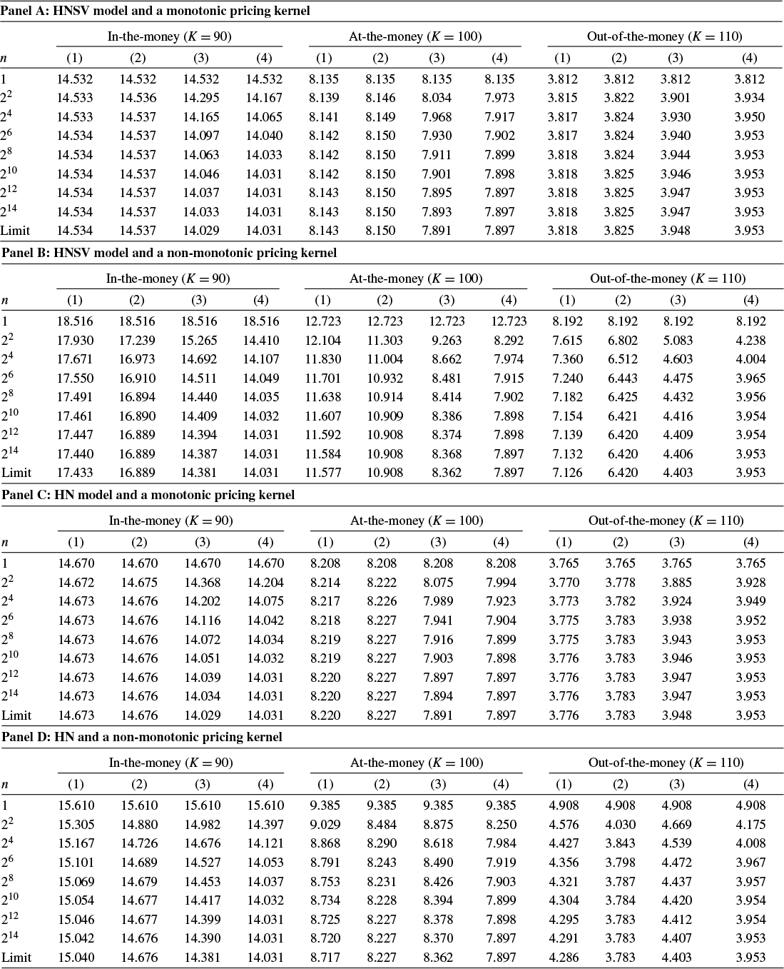
Table 2 Long description
The table is organized into four panels.
Panel A: H N S V model and a monotonic pricing kernel. For In-the-money (K = 90), prices start at 14.532 for n = 1 and converge toward a limit of 14.534 (column 1) or 14.031 (column 4). At-the-money (K = 100) prices converge from 8.135 to approximately 8.143 or 7.897. Out-of-the-money (K = 110) prices converge from 3.812 to approximately 3.818 or 3.953.
Panel B: H N S V model and a non-monotonic pricing kernel. Prices show higher initial values and more significant shifts. In-the-money prices start at 18.516 and converge to limits between 17.433 and 14.031. Out-of-the-money prices start at 8.192 and converge to limits between 7.126 and 3.953.
Panel C: H N model and a monotonic pricing kernel. Trends are similar to Panel A. In-the-money prices start at 14.670 and converge to limits between 14.673 and 14.031. Out-of-the-money prices start at 3.765 and converge to limits between 3.776 and 3.953.
Panel D: H N model and a non-monotonic pricing kernel. In-the-money prices start at 15.610 and converge to limits between 15.040 and 14.031. Out-of-the-money prices start at 4.908 and converge to limits between 4.286 and 3.953.
Across all panels, the rows for n include 1, 2 squared, 2 to the 4 power, 2 to the 6 power, 2 to the 8 power, 2 to the 10 power, 2 to the 12 power, 2 to the 14 power, and the Limit. Columns 1 through 4 represent different convergence rates for delta sub 1 and delta sub 2.
Note: This table reports one-year European call option prices for the HNSV and HN models for various strike prices as a function of the number of discretization points per day n. The HNSV model is based on
$\rho = 0.7867$
 and the HN model corresponds to
$\rho =1$
 . The other parameters are
$\lambda = 2.1257$
 ,
$\sigma ^2 = 1.2007 \times 10^{-4}$
 ,
$\phi = 0.9671$
 ,
$\alpha = 4.4440 \times 10^{-6}$
 , and
$\gamma = 1.8927 \times 10^{2}$
 . A monotonic pricing kernel is considered in Panels A and C and corresponds to
$ \xi = 0$
 , while a non-monotonic pricing kernel is considered in Panels B and D and is obtained with
$\xi = 1.6252 \times 10^4$
 . We rely on the following convergence rates for the parameters in Assumption 5: (1)
$\delta _1 = \delta _2 = 0$
 , (2)
$\delta _1 = \tfrac {1}{2}$
 ,
$\delta _2 = -\tfrac {1}{2}$
 , (3)
$\delta _1 = 0$
 ,
$\delta _2 = \tfrac {1}{2}$
 , and (4)
$\delta _1 = \tfrac {1}{2}$
 ,
$\delta _2 = \tfrac {1}{2}$
 .
When
$n = 1$
 , the prices obtained with the four convergence rate cases are identical—as expected. As soon as n increases, however, the prices become different. Their limiting values are also significantly different, which emphasizes that using different convergence rate parameters produces distinct option prices for the limiting diffusions because the underlying GARCH models converge to different diffusion limits under both the physical and risk-neutral measures. Overall, we notice that the option prices based on the weak limits obtained with the standard convergence rates from Assumption 3B are the closest to those of the underlying discrete-time model in all but one of the cases considered—in line with our theoretical results developed in Sections 3 and 4.Footnote
24
This observation thus offers another numerical justification for choosing these rates over the alternative choices from Assumption 5.
We now examine the impact on option prices of the above convergence rates relative to three key factors: the shape of the pricing kernel (monotonic vs. non-monotonic), the correlation between the innovations driving the returns and conditional variance processes (HNSV vs. HN), and the magnitude of the asymmetry parameter
$\gamma $
 .
Panels A and C of Table 2 report the monotonic pricing kernel cases; as expected, the limit prices obtained with (1) are the closest to those obtained with the GARCH model, with the maximum absolute difference being $0.008 for HNSV and $0.012 for HN. The difference is slightly larger when using the Heston and Nandi (Reference Heston and Nandi2000) convergence rates in (2); it is however significantly larger when using the rates in (3) and (4). These differences in the limit are a by-product of the dynamics given by Proposition 5 and the values of the risk-neutral long-run variance and speed of mean reversion for each limiting diffusion process.Footnote 25 Specifically, the risk-neutral variance drifts for (1) and (2) are identical under the monotonic pricing kernel, and therefore the small deviation in option prices is attributed exclusively to the difference in the variance-of-variance dynamics. The larger discrepancies between option prices computed based on (1) and (2) against (3) and (4) are mostly due to the form of the risk-neutral drift of the variance process, which changes for (1) and (2), but stays at its physical measure level for (3) and (4).
For non-monotonic pricing kernels (i.e., Panels B and D), we observe larger prices when
$n = 1$
 ; these prices decrease as n increases. As explained in Section 3.3, this pattern is caused by having larger risk-neutral conditional variances compared to the physical ones in the discrete-time models, with their ratio converging to one as n approaches infinity. As expected, the proposed rates in (1) lead to limit prices that are the closest to their GARCH counterparts, but the differences relative to the other three convergence rates are now substantial. For example, for out-of-the-money options, the differences between the HNSV and its diffusion limit prices are $1.066 for (1), $1.772 for (2), $3.789 for (3), and $4.239 for (4). The main factor which triggers these differences is the presence of the positive variance risk-preference parameter
$\xi $
 which impacts both the (risk-neutral) long-run level and speed of mean reversion of the variance process. For example, the differences in limit prices based on (1) and (2), which were rather small for monotonic pricing kernels, are now significant because the risk-neutral long-run variance level implied by (1) is larger than that obtained with (2), despite both convergence rates sharing the same mean reversion rate (see Footnote 25). In other words, when accounting for variance risk in the pricing kernel, the Heston and Nandi (Reference Heston and Nandi2000) convergence rates cannot capture the same asymptotic behavior of the risk-neutral long-run variance of the underlying HNSV model in contrast to our rates from Assumption 3B.
We now turn our attention to the effect of using different convergence rates with respect to the correlation parameter
$\rho $
 . On the one hand, we notice that for monotonic pricing kernels,
$\rho $
 does not have a large overall impact on option prices. Moreover, in the limit, it only impacts the prices obtained based on the rates used in (1) and (2). The convergence rates (3) and (4), on the other hand, are not affected by
$\rho $
 , and option prices based on their limiting diffusions are identical for the HNSV and HN models. On the other hand,
$\rho $
 has a significant effect on option prices in the non-monotonic pricing kernel case. Specifically, there is a strong negative relationship between option prices and
$\rho $
 ; for example,
$\rho =1$
 leads to a substantial overall decrease in option prices relative to the case where
$\rho = 0.7867$
 , the largest differences being documented for
$n=1$
 . For the diffusion limits, this drop is still significant but occurs only for (1) and (2). This can be explained by a decrease in the risk-neutral long-run variance level and increase in the speed of mean reversion for these two cases when
$\rho =1$
 (see again Footnote 25); as stated above,
$\rho $
 does not affect the diffusion prices resulting from (3) and (4). However, under these rates, the HNSV option prices converge very fast to their diffusion level, a substantial drop in prices occurring from
$n=1$
 to
$n=2^2$
 for all moneyness levels considered. Consequently, HN-based option prices are closer to their continuous-time limit counterparts relative to the HNSV models, in addition to being less sensitive to the choice of the convergence rate.
Finally, we investigate the behavior of the option prices based on the four convergence rates relative to different levels of the asymmetry parameter
$\gamma $
 . Figure 1 reports a graphical representation of the call option price convergence for in-the-money, at-the-money, and out-of-the-money options and four different values of
$\gamma $
 , decreasing from
$\gamma = 189.27$
 in Panel A to
$\gamma = 0$
 in Panel D. For these four cases, we report the option prices for the four convergence rates considered above, that is, (1)–(4). There is a positive relationship between the call option prices and the value of
$\gamma $
 —this is a by-product of a rise in the variance of variance and the risk-neutral long-run variance levels. In addition, we notice that the prices obtained with the diffusion limit in (1) are the closest to the original GARCH prices obtained when
$n = 1$
 , and this for all values of
$\gamma $
 considered in the figure. When
$\gamma =0$
 , the prices obtained with rates (1) and (3) are overlapping; this observation is consistent with the results of Proposition 5 and the expressions of the risk-neutral drift terms from Footnote 25. The same conclusion can be obtained for the convergence rates in (2) and (4). Interestingly, as
$\gamma $
 decreases from 189.27 to 0, we observe that the limit prices calculated using (1) and (2) approach those of (3) and (4), respectively.
Call option price convergence for the HNSV model for different values of
$\gamma $
 .
Note: This figure reports one-year European call option prices for the HNSV model for various strike prices and different values of the asymmetry parameter
$\gamma $
 , as a function of the number of discretization points per day n. The parameters are
$\lambda = 2.1257$
 ,
$\sigma ^2 = 1.2007 \times 10^{-4}$
 ,
$\phi = 0.9671$
 ,
$\alpha = 4.4440 \times 10^{-6}$
 , and
$\rho = 0.7867$
 . A non-monotonic pricing kernel with
$\xi = 1.6252 \times 10^4$
 is considered. We rely on the following convergence rates for the parameters in Assumption 5: (1)
$\delta _1 = \delta _2 = 0$
 , (2)
$\delta _1 = \tfrac {1}{2}$
 ,
$\delta _2 = -\tfrac {1}{2}$
 , (3)
$\delta _1 = 0$
 ,
$\delta _2 = \tfrac {1}{2}$
 , and (4)
$\delta _1 = \tfrac {1}{2}$
 ,
$\delta _2 = \tfrac {1}{2}$
 .

Figure 1 Long description
The image consists of four horizontal rows labeled Panel A through Panel D, each representing a different value for the asymmetry parameter gamma. Each row contains three line graphs categorized by moneyness: In-the-money (left), At-the-money (center), and Out-of-the-money (right).
All graphs share a common x-axis labeled log sub 2 (n), representing the number of discretization points per day, ranging from 0 to 14. The y-axis represents the Option price, with scales varying by panel and moneyness.
* Panel A (gamma = 189.27): Shows the highest price levels. Prices for all four convergence rates start high at n = 0 and decay toward a stable asymptote as n increases. Rate 1 (solid line) is the highest, followed by Rate 2 (dashed), Rate 3 (dotted), and Rate 4 (dash-dot) as the lowest.
* Panel B (gamma = 94.64): Displays similar downward convergence patterns but at lower absolute price levels than Panel A. The vertical spread between the four rates is narrower.
* Panel C (gamma = 47.32): The convergence curves are more tightly grouped. In the Out-of-the-money graph, the dotted line (Rate 3) and solid line (Rate 1) converge very closely at the top of the range.
* Panel D (gamma = 0): Shows the most compressed results. Only two distinct lines are visible in each graph because Rate 1 and 3 overlap (solid/dotted) and Rate 2 and 4 overlap (dashed/dash-dot), indicating that when gamma is zero, the delta parameters have symmetric effects.
A legend at the bottom center identifies the four convergence rates: (1) solid line, (2) dashed line, (3) dotted line, and (4) dash-dot line.
Collectively, these results suggest that when implementing continuous-time approximations to discrete-time option pricing models, the choice of parametric convergence rates is consequential: rates that preserve the conditional moment structure of the daily model yield the smallest pricing errors, while alternative rates can introduce systematic deviations that are amplified when the pricing kernel is non-monotonic or the leverage parameter
$\gamma $
 is large.
5.2 Empirical Calibrations
The empirical exercise of this section is designed to assess the empirical usefulness of our proposed diffusion limit. To this end, we compare the fit of the HN model with that of our diffusion limit specification obtained by setting
$\delta _1=\delta _2=0$
 using real option data. In addition, we include the Heston (Reference Heston1993) model as a benchmark. This framework allows us to compare the cross-sectional fitting ability of the proposed diffusion limit with that of the original discrete-time model and a more flexible SV model.
We retrieve the option data from OptionMetrics on the Wharton Research Data Services website. They span from January 1, 1996 to August 31, 2023. We apply a number of standard data filters, resulting in a final sample of 659,454 option prices observed over 1,429 Wednesdays. Specifically, we exclude options with non-positive trading volume or open interest, retain only those with bid prices strictly lower than ask prices and with mid-quote prices exceeding the bid-ask spread, and focus on options with maturities between one week and one year. We also remove observations with missing implied volatility or underlying price data, as well as those that violate no-arbitrage conditions. Finally, we restrict the sample to standard monthly options, excluding weekly contracts.
The comparison considers a calibration exercise in which we estimate the parameters of each model on a weekly basis. Specifically, on each Wednesday, we calibrate the model parameters by minimizing the implied volatility root mean squared error (IVRMSE) across the cross section of observed options. This approach allows the parameters to vary over time, thus capturing changes in market conditions over the nearly 28 years of our sample.
Summary statistics of implied volatility root mean squared errors across different specifications

Table 3 Long description
The table is organized into three columns for the models: H N model, H N limit, and Heston model.
Under the Moments category:
* Average: H N model is 0.0108, H N limit is 0.0104, and Heston model is 0.0088.
* Standard deviation: H N model is 0.0065, H N limit is 0.0097, and Heston model is 0.0063.
Under the Quantiles category:
* 5 super th: H N model is 0.0040, H N limit is 0.0043, and Heston model is 0.0036.
* 25 super th: H N model is 0.0062, H N limit is 0.0064, and Heston model is 0.0052.
* Median: H N model is 0.0088, H N limit is 0.0085, and Heston model is 0.0070.
* 75 super th: H N model is 0.0137, H N limit is 0.0118, and Heston model is 0.0100.
* 95 super th: H N model is 0.0241, H N limit is 0.0227, and Heston model is 0.0209.
Note: This table reports implied volatility root mean squared error (IVRMSE) for the HN model, our HN limit, and the Heston model. The HN limit uses
$\delta _1 = \delta _2 = 0$
 for the convergence rate parameters in Assumption 5. Moments and quantiles are obtained from a sample of IVRMSEs calculated on each Wednesday from January 1996 to August 2023. The option data are retrieved from OptionMetrics on the Wharton Research Data Services website. We apply a number of standard data filters, resulting in a final sample of 659,454 option prices observed over 1,429 Wednesdays.
Table 3 reports the mean and standard deviation of the weekly IVRMSEs, along with relevant quantiles of their empirical distribution, for each of the three models. The results show that, when calibrated separately, the diffusion limit of the HN model achieves a cross-sectional fit similar to that of its discrete-time counterpart, indicating that the limiting specification retains comparable empirical flexibility. Given that the Heston model offers greater flexibility than both the HN specification and its diffusion limit, we expect it to perform better on average, and our results are consistent with this expectation.
Figure 2 supplements the results of Table 3 by reporting the time series of the IVRMSEs for the three models on a semi-logarithmic plot with a logarithmic y-axis to improve readability. Overall, the Heston model exhibits lower IVRMSEs on average, indicating a better average fit over the sample. In contrast, the HN model and our proposed diffusion limit closely track each other over time, indicating that the two specifications have similar cross-sectional fitting performance.
Time series of implied volatility root mean squared errors across different specifications.
Note: This figure reports the time series of the implied volatility root mean squared error (IVRMSE) for the HN model (black solid line), our HN limit (dashed dark gray line), and the Heston model (dotted light gray line). The IVRMSEs are reported on a logarithmic scale to improve readability. The HN limit uses
$\delta _1 = \delta _2 = 0$
 for the convergence rate parameters in Assumption 5. IVRMSEs are calculated on each Wednesday from January 1996 to August 2023. The option data are retrieved from OptionMetrics on the Wharton Research Data Services website. We apply a number of standard data filters, resulting in a final sample of 659,454 option prices observed over 1,429 Wednesdays.

Figure 2 Long description
A line graph with the horizontal X axis labeled Date, ranging from 1998 to 2022 in two-year increments. The vertical Y axis is labeled Implied volatility root mean square error on a logarithmic scale with major ticks at 10 sub negative 2 and 10 sub negative 1.
Three data series are plotted:
- H N model: A solid black line.
- H N limit: A dashed dark gray line.
- Heston model: A dotted light gray line.
The data shows high volatility and frequent spikes across all models. A massive, singular peak occurs in late 2008 where all three models converge at a value slightly above 10 sub negative 1. From 1996 to 2008, the models track closely together with frequent fluctuations between 0.005 and 0.02. Post-2008, the H N model (solid black) frequently exhibits higher error peaks than the H N limit and Heston models, particularly between 2014 and 2020. Around 2020, there is another significant spike across all models, followed by a sustained higher baseline of error through 2023 compared to the pre-2008 period.
6 CONCLUDING REMARKS
This article investigates the relationship between canonical affine option pricing models in discrete and continuous time, shedding light on the discrepancies between existing results in the literature by establishing novel diffusion limits for various classes of GARCH and SV models. Using a general modeling framework which incorporates multi-component volatility, fat tails, and non-monotonic pricing kernels, we first derive weak limits for two classes of affine GARCH component models driven by Gaussian and inverse Gaussian innovations, and risk-neutralized with an exponential linear pricing kernel. These limits coincide if some relationships between the two models’ parameters are satisfied. When restricted to a single volatility component, our limits generalize the result of Heston and Nandi (Reference Heston and Nandi2000) in the Gaussian case and provide an alternative pathway to obtain the inverse Gaussian limiting process of Christoffersen et al. (Reference Christoffersen, Heston and Jacobs2006). In contrast to these studies, which recover limiting processes governed by a single noise, our weak limits correspond to two-dimensional non-degenerate diffusions driven by stochastically correlated Brownian motions. This discrepancy arises due to the use of different asymptotic assumptions on the model parameters, leading to our subsequent contribution: the characterization of all possible limits for two classes of affine and non-affine discrete-time SV models. Interestingly, both specifications converge to affine diffusion limits and our asymptotic rates lead to the most complex dynamics sharing the same statistical properties as their discrete-time counterparts. Numerical experiments involving European options suggest that our limiting diffusions provide the closest prices to their daily discrete-time counterparts. In addition, we find that the correlation between the underlying innovations and the shape of the pricing kernel are the two main determinants of the convergence behavior.
Our work can be extended in several possible ways. For example, weak limits can be further generalized to other discrete-time affine frameworks including jumps or information on the realized variance (RV), such as the Lévy GARCH model of Ornthanalai (Reference Ornthanalai2014), the generalized affine RV model of Christoffersen et al. (Reference Christoffersen, Feunou, Jacobs and Meddahi2014), the heterogeneous autoregressive gamma model of Corsi, Fusari, and La Vecchia (Reference Corsi, Fusari and La Vecchia2013), and its extensions (see, e.g., Majewski et al., Reference Majewski, Bormetti and Corsi2015; Alitab et al., Reference Alitab, Bormetti, Corsi and Majewski2020; Bormetti et al., Reference Bormetti, Casarin, Corsi and Livieri2020). While we primarily discuss applications to European option pricing, our weak limits could also be considered to examine the convergence of hedge ratios or optimal portfolio policies, as well as for pricing other derivatives (e.g., exotic options and volatility derivatives). Finally, our results linking discrete-time non-affine models to affine diffusions should be further investigated both theoretically and empirically. A potential area for future research could involve leveraging this relationship to enhance the efficiency of pricing and hedging in non-affine discrete-time settings using established methods and closed-form solutions available for affine diffusions.
A APPENDIX
A.1 Affine Representations for the Discretized HN(C) and IG(C) Models
Following straightforward algebraic manipulations, we can show that for the HN(C) case, the
$\mathcal {F}^{(n)}_{k\tau }$
 -conditional joint cgf of
$\Delta Y^{(n)}_{(k+1)\tau }$
 ,
$\Delta s^{(n)}_{(k+1)\tau }$
 , and
$\Delta q^{(n)}_{(k+1)\tau }$
 evaluated at w and
$\boldsymbol {v} = \left [ \,\, v_1 \quad v_2 \,\, \right ]^{\top }$
 follows Equation (6) with the following one-step coefficients:


where
$\odot $
 represents the Hadamard (element-wise) product.
Similarly, for the IG(C) model, the
$\mathcal {F}^{(n)}_{k\tau }$
 -conditional joint cgf of
$\Delta Y^{(n)}_{(k+1)\tau }$
 ,
$\Delta s^{(n)}_{(k+1)\tau }$
 , and
$\Delta q^{(n)}_{(k+1)\tau }$
 follows Equation (6) with


A.2 Proofs of Propositions 2 and 3
The proofs of Propositions 2 and 3 rely on the weak convergence theorem for Markov processes stated by Nelson (Reference Nelson1990) and restated as Theorem SM.1 in the Supplementary Material. Applying this theorem requires verifying three conditions. Conditions (i) and (ii) concern the limiting drift vector and covariance matrix per unit of time. Specifically, for any fixed
$\boldsymbol {x}$
 and any given time
$k\tau $
 , one must show that

where we use the fact, noted in Nelson (Reference Nelson1990), that the difference between the conditional second-moment matrix and the conditional covariance matrix vanishes as
$\tau \to 0$
 , so that it suffices to work with the latter. Since the conditional first- and second-moment functions are affine in
$\boldsymbol {x}$
 , convergence of the coefficients in their affine representations implies uniform convergence over compact subsets of the state domain, as required by conditions (i) and (ii). Condition (iii) imposes a bound on conditional moments of order
$2+\delta $
 for some
$\delta>0$
 , which ensures that large increments are negligible asymptotically and hence that the sample paths of the limiting process are continuous with probability one.
Before turning to the specific proofs, we present in Appendix A.2.1 a general method for computing the required conditional mean vector and covariance matrix of
$\Delta \boldsymbol {X}^{(n)}_{(k+1)\tau }$
 and their limits per unit of time. The method exploits the affine structure of the
$\mathcal {F}^{(n)}_{k\tau }$
 -conditional cgf stated in Assumption 1 and applies regardless of the distributional specification
$\mathcal {D}$
 or the underlying probability measure. For brevity, the approach is illustrated under the physical measure as the procedure under the risk-neutral measure is entirely analogous and is therefore omitted.
A.2.1 A General Method for the Computation of the Drift and Diffusion Terms
The first- and second-order conditional moments of
$\Delta \boldsymbol {X}^{(n)}_{(k+1)\tau } = \big [\,\Delta Y^{(n)}_{(k+1)\tau }\;\; \Delta s^{(n)}_{(k+1)\tau }\;\; \Delta q^{(n)}_{(k+1)\tau }\,\big ]^{\top }$
 are recovered from the joint cumulants of the process, which are obtained as partial derivatives of the
$\mathcal {F}^{(n)}_{k\tau }$
 -conditional joint cgf of
$ \Delta \boldsymbol {X}^{(n)}_{(k+1)\tau }$
 evaluated at
$\boldsymbol {0}$
 . Specifically, for any real vector
$\boldsymbol {x} = \big [\,\,x_1\quad x_2\quad x_3\,\,\big ]^\top $
 and
$l,m \in \{1,2,3\}$
 , we have

where
$\mathcal {C}^{\mathbb {P}^{(n)}}\big (\boldsymbol {x} \,\big |\, \mathcal {F}^{(n)}_{k\tau }\big )$
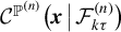 is the cgf of
$ \Delta \boldsymbol {X}^{(n)}_{(k+1)\tau }$
 , which admits the affine representation of Equation (6) from Assumption 1. By this affine structure, computing partial derivatives of this cgf reduces to differentiating its coefficients
$\mathcal {A}^{\mathcal {D}}$
 and
$\mathcal {B}^{\mathcal {D}}_{u}$
 for
$u\in \{s,q\}$
 .
We introduce the following notation for the first- and second-order partial derivatives for the coefficients of the
$\mathcal {F}^{(n)}_{k\tau }$
 -conditional cgf of
$ \Delta \boldsymbol {X}^{(n)}_{(k+1)\tau }$
 from Assumption 1 evaluated at
$w=0$
 and
$\boldsymbol {v} = \boldsymbol {0}$
 . For any nonnegative integers
$i, j, k$
 with
$1\leq i+j+k \leq 2$
 , and
$u\in \{s,q\}$
 , we let


The drift vector and the covariance matrix of the weak limit are then obtained by dividing these quantities by
$\tau $
 and passing to the limit. This is achieved by computing

using the convergence rates assumed for the model parameters. Note that these rates have been chosen such that these limits exist and are finite, that is,
$ \mathcal {A}^{\mathcal {D}}_{i,j,k}< \infty $
 and
$\mathcal {B}^{\mathcal {D}}_{u,i,j,k} < \infty $
 . By the affine form of the cgf, the drift coefficient of Equation (17) is given by

The
$3 \times 3$
 positive semidefinite matrix of asymptotic second-order cross-cumulants is denoted by
$\boldsymbol {B}^{\mathcal {D}}(\boldsymbol {X}_t) = \left (B^{\mathcal {D}}_{rl}(\boldsymbol {X}_t)\right )$
 , with
$r, l \in \{1,2,3\}$
 . Since under both cgf specifications of Appendix A.1, we have
$\mathcal {B}^{\mathcal {D}}_{s,i,j,k} = \mathcal {B}^{\mathcal {D}}_{q,i,j,k}$
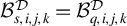 , for any
$i+j+k = 2$
 , each entry of matrix
$\boldsymbol {B}^{\mathcal {D}}(\boldsymbol {X}_t)$
 is linear in
$h_t$
 , so that

Using the Cholesky decomposition of matrix
$\boldsymbol {B}^{\mathcal {D}}\left (\boldsymbol {X}_t\right ) = \left ( \boldsymbol {\Sigma }^{\mathcal {D}}\left (\boldsymbol {X}_t\right ) \right ) \left (\boldsymbol {\Sigma }^{\mathcal {D}}\left (\boldsymbol {X}_t\right )\right )^\top $
 , where
$\boldsymbol {\Sigma }^{\mathcal {D}}(\boldsymbol {X}_t)$
 is a lower triangular matrix representing the diffusion of the GARCH weak limit of Equation (17), we obtain

A.2.2 Proof of Proposition 2
The proof follows the approach described at the start of this appendix and proceeds by verifying conditions (i)–(iii) of Theorem SM.1 in the Supplementary Material. Conditions (i) and (ii) are established from the limiting conditional mean and covariance matrix of
$\Delta \boldsymbol {X}^{(n)}_{(k+1)\tau }$
 , while condition (iii) is verified separately. We first derive the weak limit for the HN(C) model. The corresponding derivation for the IG(C) model follows in a similar way and is provided in Section SM.D.2 of the Supplementary Material.
Following the methodology of Appendix A.2.1 and using the definitions of Equations (A.7) and (A.8), we proceed by evaluating the partial derivatives of the step dependent coefficients of Equations (A.1)–(A.3) at
$w=0$
 and
$\boldsymbol {v}=\boldsymbol {0}$
 and compute their limits per discretization step under the constraints from Assumption 3A. For any
$u \in \{s,q\}$
 , we obtain the following first-order quantities:

Replacing the above quantities into the general drift term of Equation (A.10) allows us to obtain

Next, for
$u \in \{s,q\}$
 , we compute the limits of the second-order derivatives per discretization step using the convergence rates of Assumption 3B:

Plugging these into the matrix of asymptotic second-order cross-cumulants of Equation (A.11) leads to

Performing the Cholesky decomposition of the covariance matrix of Equation (A.13) as outlined in Equation (A.12), we obtain the diffusion term

The resulting limit is a degenerate diffusion driven by two mutually independent Brownian motions
$W_{1}$
 and
$W_{2}$
 . This is a consequence of the diffusion matrix
$\boldsymbol {\Sigma }^{\mathcal {N}}\left (\boldsymbol {X}_t\right )$
 having a unique representation along with a column of zeros—a direct consequence of the matrix
$\boldsymbol {B}^{\mathcal {N}}\left (\boldsymbol {X}_t\right )$
 being singular and of rank two.
Next, we need to verify Condition (iii) of Theorem SM.1 in Section SM.A of the Supplementary Material that there exists a
$\delta>0$
 such that

Indeed, if we let
$\delta = 2$
 and take the fourth-order derivatives of the moment generating function of
$\Delta \boldsymbol {X}^{(n)}_{(k+1)\tau }= \big [\,\,\Delta Y^{(n)}_{(k+1)\tau }\quad \Delta s^{(n)}_{(k+1)\tau }\quad \Delta q^{(n)}_{(k+1)\tau }\,\,\big ]^\top $
 conditional on
$\mathcal {F}^{(n)}_{k\tau }$
 , we can show that

where
$L^{\mathcal {N}}_Y$
 ,
$L^{\mathcal {N}}_s$
 , and
$L^{\mathcal {N}}_q$
 are finite quantities which depend on
$ \boldsymbol {X}^{(n)}_{k\tau }$
 and its diffusion limit parameters, specifically we have
$L^{\mathcal {N}}_Y = 3\left (h^{(n)}_{k\tau }\right )^2$
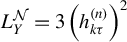 and
$L^{\mathcal {N}}_u = 12 \alpha ^4_u\left (5+20\gamma ^2_uh_{k\tau }+4\gamma ^4_u \left (h^{(n)}_{k\tau }\right )^2\right )$
 , for
$u\in \{s,q\}$
 .
We now proceed to verify if the multidimensional Feller constraints of Duffie and Kan (Reference Duffie and Kan1996) are satisfied by the HN(C) diffusion limit. A sufficient condition for the existence and uniqueness of a (strong) solution to our diffusion limit is given below.
Condition 1. (Sufficient Condition for the Existence of a Solution of the Affine SDE)
-
A. For all $\boldsymbol {x}$
such that
$V_i\left (\boldsymbol {x}\right ) = 0$
, we have
$\boldsymbol {v}^\top _{1,i} \left ( \boldsymbol {A}_0 + \boldsymbol {A}^{\mathcal {N}}_1\boldsymbol {x} \right )> \dfrac {1}{2}\boldsymbol {v}^\top _{1,i}\boldsymbol {\Gamma }^{\mathcal {N}}\left (\boldsymbol {\Gamma }^{\mathcal {N}}\right )^\top \boldsymbol {v}_{1,i}$
. -
B. For all j, if $\left (\boldsymbol {v}^\top _{1,i}\boldsymbol {\Gamma }^{\mathcal {N}}\right )_j \neq 0$
, then
$V_i\left (\boldsymbol {x}\right ) $
and
$V_j\left (\boldsymbol {x}\right ) $
are proportional.



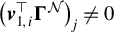


Part A of Condition 1 ensures that each volatility process
$V_i\left (\boldsymbol {x}\right )$
 has a strong positive drift at the boundary
$V_i\left (\boldsymbol {x}\right ) = 0$
 . The above inequality typically imposes a constraint on the model parameters, as explained below. First, we notice that when
$i=2,3$
 ,
$V_i\left (\boldsymbol {x}\right ) =1>0$
 , so we only need to analyze the case when
$i=1$
 . The boundary constraint corresponds to having
$s_t = -q_t$
 , so the inequality in Part A becomes

Since
$\kappa _s>\kappa _q$
 , the preceding inequality is satisfied on the portion of the boundary where
$q_t>0$
 whenever

For the one-component HN limit, the corresponding restriction in Part A reduces to
$\kappa \sigma ^2> \alpha ^2 + 2\alpha ^2\gamma ^2$
 . Although these parameter restrictions may limit the flexibility of the models, they could be imposed during estimation. According to Duffie and Kan (Reference Duffie and Kan1996), Part B of Condition 1 implies that whenever the
$i^{\text {th}}$
 volatility is at zero, it cannot be driven “negative” by dependence on other nonzero volatilities. This condition is automatically satisfied for
$i=2,3$
 , so we only need to verify the case
$i=1$
 . We notice that
$\left (\boldsymbol {v}^\top _{1,1}\boldsymbol {\Gamma }^{\mathcal {N}}\right )_3 =0$
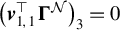 and, because
$V_1\left (\boldsymbol {x}\right ) $
 and
$V_2\left (\boldsymbol {x}\right ) $
 are not proportional, we need
$\left (\boldsymbol {v}^\top _{1,1}\boldsymbol {\Gamma }^{\mathcal {N}}\right )_2 = \sqrt {2}\left (\alpha _s + \alpha _q\right ) = 0$
 , which implies that
$\alpha _s = -\alpha _q$
 . This condition is rather restrictive and it is not typically consistent with the parameter values used in the literature, as the majority of the research papers on pricing under GARCH component models impose both ARCH coefficients to be nonnegative. Finally, we notice that in the HN case, Part B of Condition 1 is satisfied by our diffusion limit only if we take
$\alpha = 0$
 , which corresponds to a deterministic volatility case.
A.2.3 Proof of Proposition 3
The main characteristic of the pricing kernel of Assumption 2 is that it preserves the affine property of Assumption 1 after the change of measure is applied. Indeed, it is straightforward to show that for any real w and
$\boldsymbol {v} = \left [ \,\, v_1 \quad v_2 \,\, \right ]^{\top }$
 , the joint cgf of
$ \Delta Y^{(n)}_{(k+1)\tau }$
 ,
$ \Delta s^{(n)}_{(k+1)\tau }$
 , and
$\Delta q^{(n)}_{(k+1)\tau }$
 conditional on
$\mathcal {F}^{(n)}_{k\tau }$
 has the following affine representation under the risk-neutral measure
$\mathbb {Q}^{(n)}$
 :

where the coefficients
$\tilde {\mathcal {A}}^{\mathcal {D}}\left (w, \boldsymbol {v}; \tau \right )$
 and
$\tilde {\mathcal {B}}^{\mathcal {D}}_u\left (w, \boldsymbol {v}; \tau \right )$
 satisfy the following relationships:


for
$ u \in \{s,q\}$
 . Therefore, the process for deriving the risk-neutral weak limits is based on the approach detailed in Appendix A.2.1 but adapted for this specific probability measure. We remark that it is not necessary to derive the risk-neutral dynamics to compute our diffusion limit under the
$\mathbb {Q}$
 measure.
The risk-neutral limit for the HN(C) model is derived as follows. First, using the approach of Augustyniak et al. (Reference Augustyniak, Badescu and Bégin2023), we solve the martingale constraints in Equations (8) and (9) based on the coefficients of the
$\mathcal {F}^{(n)}_{k\tau }$
 -conditional joint cgf of
$ \Delta Y^{(n)}_{(k+1)\tau }$
 ,
$ \Delta s^{(n)}_{(k+1)\tau }$
 , and
$\Delta q^{(n)}_{(k+1)\tau }$
 under
$\mathbb {P}^{(n)}$
 computed in Equations (A.1)–(A.3). We obtain the following relationship between the risk preference parameters
$\theta (\tau )$
 and
$\boldsymbol {\xi }(\tau )$
 :

Under the limiting parameter constraints of Assumptions 3 and 4, the limit of the equity risk preference parameter exists and is given by

Second, we introduce the first- and second-order partial derivatives for the risk-neutral cgf coefficients and express them in terms of the physical quantities using Equations (A.15) and (A.16). Thus, for any nonnegative integers
$i, j, k$
 with
$1\leq i+j+k \leq 2$
 , and
$u\in \{s,q\}$
 , we have


Using Equations (A.17) and (A.18), and the limiting parameter constraints of Assumptions 3 and 4, we compute the first-order limits. To lighten the notation, we set

and we note that
$\lim \limits _{\tau \to 0} \tau ^{-\frac {1}{2}} R(\tau ) = -\left (\lambda + \frac {1}{2}\right )$
 and
$\lim \limits _{\tau \to 0} \left (1 - 2 \boldsymbol {\alpha }(\tau )^\top \boldsymbol {\xi }(\tau )\right ) = 1$
 , which explains the limiting values obtained below:

Replacing these quantities into Equation (A.10) allows us to obtain the risk-neutral drift coefficient from Equation (26). For any
$u \in \{s,q\}$
 , we now compute the second-order limits using Equations (A.17) and (A.18) together with the convergence rates of Assumptions 3B and 4:

Plugging these values into the matrix of asymptotic second-order cross-cumulants of Equation (A.11) leads to the same covariance matrix as under the physical measure, so that
$ \tilde { \boldsymbol {\Sigma }}^{\mathcal {N}}\left (\boldsymbol {X}_t\right ) = \boldsymbol {\Sigma }^{\mathcal {N}}\left (\boldsymbol {X}_t\right )$
 . Condition (iii) of Theorem SM.1 (see Section SM.A of the Supplementary Material) and the multidimensional Feller constraints of Duffie and Kan (Reference Duffie and Kan1996) are verified in the same way as in Appendix A.2.2.
SUPPLEMENTARY MATERIAL
Augustyniak, M., Badescu, A., Bégin, J.-F., & Jayaraman, S. K. (July 2026): Supplement to “On the relation between discrete- and continuous-time affine option pricing models,” Econometric Theory Supplementary Material. To view, please visit: https://doi.org/10.1017/S0266466626100607.
FUNDING STATEMENT
Financial support from the Natural Sciences and Engineering Research Council of Canada (NSERC) is gratefully acknowledged by M.A., A.B., and J.-F.B. J.-F.B. also wishes to thank the financial support of Simon Fraser University.
COMPETING INTEREST STATEMENT
The authors declare that no competing interests exist.


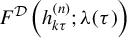





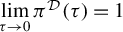

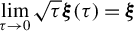







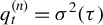



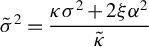



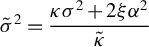


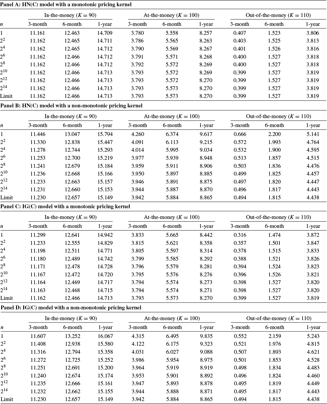
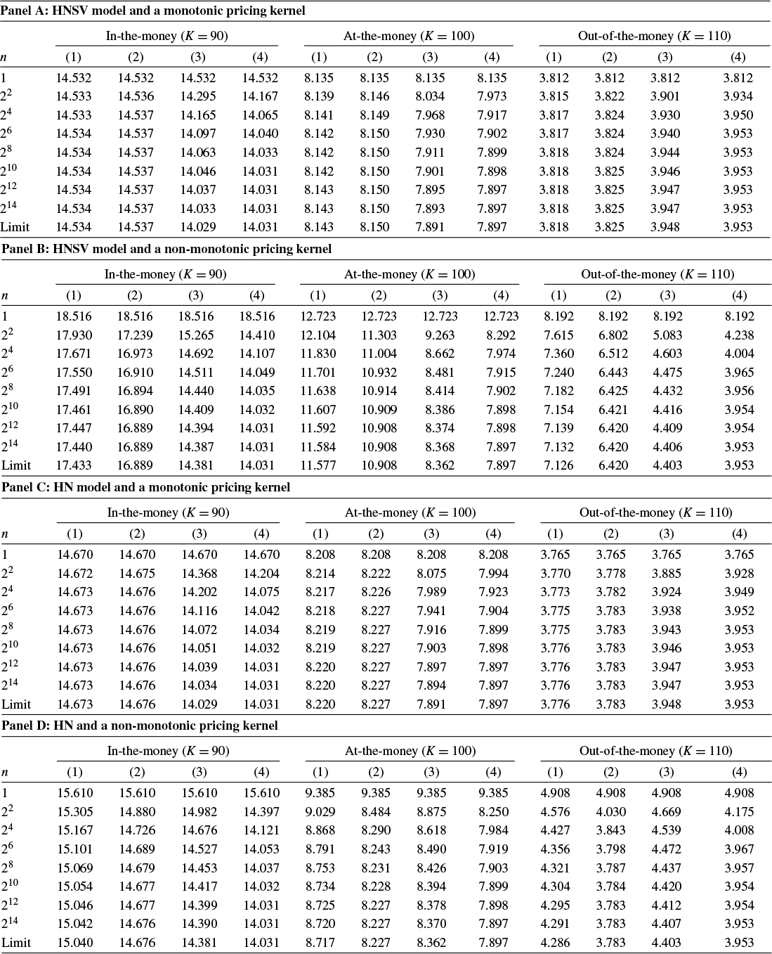
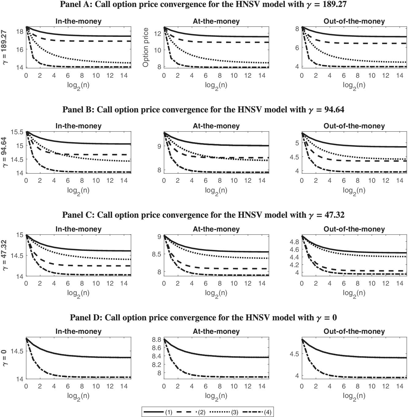


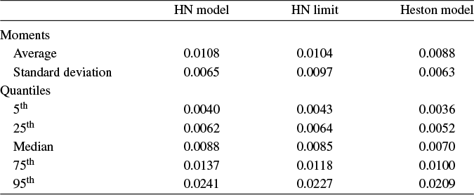
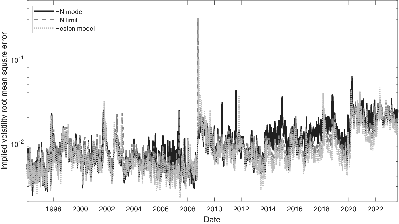


 Open access

