


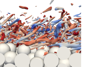





1. Introduction
Flow and transport over rough and permeable interfaces are relevant in a wide range of natural and industrial systems. A prominent example is the uppermost layer of a river bed, the hyporheic zone, which plays a vital role in aquatic ecosystems. In the hyporheic zone, the water in the pore space of the sediment is in permanent interaction with the overlying turbulent stream flow via bidirectional exchange of mass and momentum (e.g. Boano et al. Reference Boano, Harvey, Marion, Packman, Revelli, Ridolfi and Wörman2014). Due to the high biogeochemical activity within the hyporheic zone, the supply and removal of different substances by hyporheic mass transport is critical for the metabolism of various microorganisms (Brunke & Gonser Reference Brunke and Gonser1997; Battin et al. Reference Battin, Besemer, Bengtsson, Romani and Packmann2016). Advances in the fundamental understanding of the hydrodynamics near the sediment–water interface are of interdisciplinary interest (Krause et al. Reference Krause, Hannah, Fleckenstein, Heppell, Kaeser, Pickup, Pinay, Robertson and Wood2011; Ward Reference Ward2016), and are likely transferrable to similar cases of turbulent flow over dense porous media of granular material.
Moving downward from the free surface, several layers can be identified in the fully developed flow over rough and permeable beds (Nikora et al. Reference Nikora, Goring, McEwan and Griffiths2001). The undisturbed free flow region contains the outer layer. If inner length scales are small in comparison with the flow depth and the Reynolds number is sufficiently high, a logarithmic layer can emerge. According to Nikora et al. (Reference Nikora, Goring, McEwan and Griffiths2001), the roughness layer comprises two sublayers: the form-induced sublayer refers to a region above the roughness crests, where the flow is indirectly influenced via dispersive stresses, which are also referred to as form-induced stresses. In the interfacial sublayer, the flow is directly affected by the action of drag exerted by the individual sediment grains. In the subsurface layer, the flow velocity reduces to its value determined by an equilibrium between volume forces and drag, as described by Darcy's equation.
For turbulent flow over a flat sediment bed, the following dimensionless numbers are commonly used to characterize the flow in the different regions (Breugem, Boersma & Uittenbogaard Reference Breugem, Boersma and Uittenbogaard2006; Voermans, Ghisalberti & Ivey Reference Voermans, Ghisalberti and Ivey2017). The outer flow and turbulence profiles primarily depend on the friction Reynolds number  $Re_\tau =u_\tau h/\nu$, based on the friction velocity
 $u_\tau$, the water depth
 $h$ and the kinematic viscosity
 $\nu$. Near the surface of the sediment bed, the roughness length scale
 $k_s$ and the permeability
 $K$ are expected to be relevant parameters, which motivates a description by means of the roughness Reynolds number
 $Re_{k_s}=u_\tau k_s/\nu = k_s^+$ and the permeability Reynolds number
 $Re_K=u_\tau \sqrt {K}/\nu$. The parameters
 $Re_K$ and
 $Re_{k_{s}}$ are connected via the geometric structure of the sediment bed. Particularly for granular porous media with a narrow grain size distribution, the effects of roughness and permeability are tightly linked (Voermans et al. Reference Voermans, Ghisalberti and Ivey2017; Shen, Yuan & Phanikumar Reference Shen, Yuan and Phanikumar2020; Karra et al. Reference Karra, Apte, He and Scheibe2023). The roughness regime can be identified by the roughness Reynolds number
 $k_s^+$ (Raupach, Antonia & Rajagopalan Reference Raupach, Antonia and Rajagopalan1991; Jiménez Reference Jiménez2004; Kadivar, Tormey & McGranaghan Reference Kadivar, Tormey and McGranaghan2021). In the dynamically smooth regime (
 $k_s^+ < 5$), primarily viscous stresses are responsible for the momentum transfer to the solid surface. For
 $k_s^+ > 70$, the dynamically fully rough regime, the pressure drag on the roughness elements governs the interaction between the flow and the solid surfaces. The transitionally rough regime is found between both extremes. The permeability regime is characterized by the permeability Reynolds number
 $Re_K$ (Breugem et al. Reference Breugem, Boersma and Uittenbogaard2006; Manes, Poggi & Ridolfi Reference Manes, Poggi and Ridolfi2011; Voermans et al. Reference Voermans, Ghisalberti and Ivey2017; Karra et al. Reference Karra, Apte, He and Scheibe2023). As the square root of the permeability
 $\sqrt {K}$ can be seen as an effective pore diameter, high values (
 $Re_K \gg 1$) indicate that turbulent motion is likely to entrain into the pore space of a highly permeable boundary. Low values of (
 $Re_K \ll 1$) are associated with nearly impermeable boundaries and were studied in Rosti, Cortelezzi & Quadrio (Reference Rosti, Cortelezzi and Quadrio2015). The range of
 $Re_K \approx 1\unicode{x2013}2$ was identified as a transition between both extremes. As it purely depends on the key parameter
 $Re_K$, the hydrodynamic framework of Voermans et al. (Reference Voermans, Ghisalberti and Ivey2017) does not consider the absolute value of the permeability. Considering the effect of surface roughness, however, Manes et al. (Reference Manes, Poggi and Ridolfi2011) pointed out that the flow over granular beds may differ substantially from the flow over plant canopies or open-cell foams, which combine low surface roughness and high permeability.
To describe the flow over rough and permeable walls in either inner or outer coordinates, a zero level of the bed-normal coordinate  $z$ must be defined. Different approaches have been outlined. Geometrical properties of the porous medium can act as a first reference point. Examples include the crests of the topmost sediment grains (e.g. Goharzadeh, Khalili & Jørgensen Reference Goharzadeh, Khalili and Jørgensen2005), the inflection point of the porosity profile (e.g. Voermans et al. Reference Voermans, Ghisalberti and Ivey2017) or the average measured bed elevation (e.g. Mignot, Barthelemy & Hurther Reference Mignot, Barthelemy and Hurther2009). A dynamical zero level can be defined as the position where the drag acts on the roughness elements, as proposed by Thom (Reference Thom1971). Jackson (Reference Jackson1981) provided theoretical support for this idea, and noted that this position also represents a displacement height for the total shear stress. Later, Breugem et al. (Reference Breugem, Boersma and Uittenbogaard2006) modified the approach of Jackson (Reference Jackson1981) to make it applicable for flows driven by mean pressure gradients. Another approach is to derive a zero level from properties of the mean velocity profiles above the permeable wall. As demonstrated by Breugem et al. (Reference Breugem, Boersma and Uittenbogaard2006) and Suga et al. (Reference Suga, Matsumura, Ashitaka, Tominaga and Kaneda2010), a displacement height is determined such that a plateau in the diagnostic function results where the logarithmic region is expected. This technique yields values for the roughness length and for the von Kármán coefficient
 $\kappa$. Several studies applied this log-fitting approach to flows over permeable walls (e.g. Fang et al. Reference Fang, Han, He and Dey2018; Shen et al. Reference Shen, Yuan and Phanikumar2020), and found von Kármán coefficients significantly below the default value of
 $\kappa \approx 0.4$. According to Manes et al. (Reference Manes, Poggi and Ridolfi2011), however, insufficient inner–outer scale separation may distort the logarithmic layer. Yao, Chen & Hussain (Reference Yao, Chen and Hussain2022) report that a friction Reynolds number of
 $Re_\tau > 2000$ is required to obtain a logarithmic layer. Chen & García-Mayoral (Reference Chen and García-Mayoral2023) criticize that the log-fitting approach depended on the assumed extent of the logarithmic region and that it would not ensure outer-layer similarity. They propose to determine the zero-plane displacement height by minimizing the differences between the smooth-wall diagnostic function and the diagnostic function of the flow profile over a canopy, considering all regions above the roughness sublayer. Accordingly, the method of Chen & García-Mayoral (Reference Chen and García-Mayoral2023) relies on the concept of wall similarity. Townsend (Reference Townsend1976) postulated Reynolds number similarity, from which Raupach et al. (Reference Raupach, Antonia and Rajagopalan1991) derived the wall similarity hypothesis, stating that far-wall turbulent motion exclusively depends on outer-scale variables. The underlying dimensional arguments, however, demand a sufficiently high Reynolds number and a separation between inner and outer scales. Chung et al. (Reference Chung, Hutchins, Schultz and Flack2021) summarized that outer-layer similarity must be given to obtain a logarithmic layer in the overlap region, whereas outer-layer similarity can still be observed in the wake region, even if a logarithmic layer is absent.
The transition layer between the free flow and the Darcy regime takes place in the so-called Brinkman layer, whose thickness establishes an interface length scale. Goharzadeh et al. (Reference Goharzadeh, Khalili and Jørgensen2005) identified the grain diameter as a good approximation of the Brinkman-layer thickness. Voermans et al. (Reference Voermans, Ghisalberti and Ivey2017), Fang et al. (Reference Fang, Han, He and Dey2018) and Karra et al. (Reference Karra, Apte, He and Scheibe2023) reported that the Brinkman-layer thickness depends on  $Re_K$. To investigate similarities between different types of porous media, Ghisalberti (Reference Ghisalberti2009) used a drag length scale, which is correlated with the penetration depth of shear. Similarly, Manes et al. (Reference Manes, Poggi and Ridolfi2011) suggested deriving a length scale from the shear penetration depth, which also increases with
 $Re_K$. The boundary condition formulated by Beavers & Joseph (Reference Beavers and Joseph1967) relies on an interface length scale relating the interface velocity to its gradient, which emphasizes the importance of the parameter.
Increasing permeability reduces the shear intensity and relaxes the wall-blocking effect, which affects the structure of turbulence (e.g. Breugem et al. Reference Breugem, Boersma and Uittenbogaard2006; Rosti et al. Reference Rosti, Cortelezzi and Quadrio2015; Suga, Nakagawa & Kaneda Reference Suga, Nakagawa and Kaneda2017): with increasing  $Re_K$, bed-normal and lateral velocity fluctuations gain intensity, whereas streamwise velocity fluctuations decrease. At the same time, elongated high- and low-velocity streaks as well as quasi-streamwise vortices were found to vanish. Large shear instability vortices were observed in the flow over highly permeable walls such as plant canopies (Breugem et al. Reference Breugem, Boersma and Uittenbogaard2006; Finnigan Reference Finnigan2000). Manes et al. (Reference Manes, Poggi and Ridolfi2011) concluded that attached eddies are predominantly responsible for momentum exchange in flow over walls of low or intermediate permeability, where the shear entrainment depth is small compared with the boundary layer thickness. For intermediate permeability, Suga, Mori & Kaneda (Reference Suga, Mori and Kaneda2011) outlined a conceptional scenario for vortex development. The legs of a hairpin vortex entrain into the porous medium, where they lose energy and decay. The head of the hairpin vortex remains and develops as a transverse vortex. At
 $Re_K = 24.2$, Lian et al. (Reference Lian, Dallmann, Sonin, Roche, Packman, Liu and Wagner2021) observed grain-scale horseshoe vortices on the upstream face of top-layer spheres, from where they were either ejected into the flow above or forced into the pore space. For lower
 $Re_K$, Fang et al. (Reference Fang, Han, He and Dey2018) concluded that the wall blocking effect preserves small recirculation regions in recesses between spheres, which reduced the vertical Reynolds normal stresses.
This overview emphasizes the relevance of the interface definition as well as the identification of a characteristic interfacial length scale. The existence of multiple and partially conflicting approaches indicates that these questions have not been answered conclusively. Other findings underline that permeability and roughness influence the turbulence structure, which could help to explain changes in the overall flow behaviour. Accordingly, the present study addresses the following questions: (i) Is there a consistent interface definition which allows both an inner and outer scaling of primary flow variables? (ii) How does the combined effect of roughness and permeability influence the near-interface flow, and does this influence reach into the outer layer? (iii) How do roughness and permeability influence turbulence structure, i.e. near-wall streaks, anisotropy and vortex orientation? To answer these question, we investigate turbulent open-channel flow over a random sphere pack by means of pore-resolved direct numerical simulation (DNS) systematically varying  $Re_\tau$ and
 $Re_K$. The applied methods are introduced in § 2, before details of the simulations are presented in § 3. Section 4 documents the main results, and § 5 contains a discussion of the findings. A conclusion in § 6 summarizes the outcomes of the study.
2. Methodology
After the introduction of the governing equations, we describe the employed numerical methods in § 2.2. The double-averaging analysis framework is outlined in § 2.3.
2.1. Governing equations
We use DNS to solve the Navier–Stokes equations for an incompressible Newtonian fluid with a density  $\rho$ and a kinematic viscosity
 $\nu$. Using the Einstein summation convention, the conservation of mass and momentum read
 $$\begin{gather} \frac{\partial u_i}{\partial x_i} = 0, \end{gather}$$
 $$\begin{gather}\frac{\partial u_i}{\partial t} + u_j \frac{\partial u_i}{\partial x_j} =- \frac{1}{\rho} \frac{\partial p}{\partial x_i} + \nu \frac{ \partial^2 u_i }{ \partial x_j \partial x_j } + g_i. \end{gather}$$
With  $x_1 \equiv x$, we refer to the streamwise direction, while
 $x_2 \equiv y$ represents the spanwise direction and
 $x_3 \equiv z$ is the bed-normal coordinate. Accordingly,
 $u_1 \equiv u$,
 $u_2 \equiv v$ and
 $u_3 \equiv w$ represent the flow velocities into these directions, whereas
 $p$ is the pressure and
 $g_i$ is a volume force acting on the fluid.
2.2. Numerical methods
We used our in-house code MGLET (Manhart, Tremblay & Friedrich Reference Manhart, Tremblay and Friedrich2001; Manhart Reference Manhart2004; Peller et al. Reference Peller, Duc, Tremblay and Manhart2006; Sakai et al. Reference Sakai, Mendez, Strandenes, Ohlerich, Pasichnyk, Allalen and Manhart2019), which employs an energy-conserving central second-order finite volume method. The variables are defined at staggered positions within Cartesian grids on different refinement levels. This multi-level approach allows for a local grid refinement (Manhart Reference Manhart2004). The time integration is accomplished by an explicit third-order low-storage Runge–Kutta method (Williamson Reference Williamson1980). The flow solver represents the complex geometry of the resolved pore space by means of an immersed boundary representation (Peller et al. Reference Peller, Duc, Tremblay and Manhart2006; Peller Reference Peller2010). The no-slip boundary condition on the solid–fluid interface is imposed by a ghost-cell approach, which reaches second-order spatial accuracy while it ensures mass conservation (Peller Reference Peller2010). The simulation code MGLET was fine tuned in terms of load distribution, usage of vector operations and efficient parallel I/O operations to increase computational efficiency on modern computer hardware (Sakai et al. Reference Sakai, Mendez, Strandenes, Ohlerich, Pasichnyk, Allalen and Manhart2019).
We verified the accuracy order of our numerical method by simulating a laminar flow through a mono-disperse random sphere pack within a minimalistic  $x$–
 $y$-periodic domain of
 $2.5D \times 2.5D \times 4.0D$. The cell side length
 $\Delta x$ of the cubical cells was systematically refined. At contact points between spheres, the infinitesimally narrow fluid gap cannot be resolved by commonly used spatial discretization methods (Finn & Apte Reference Finn and Apte2013; Unglehrt & Manhart Reference Unglehrt and Manhart2022). To ensure convergence against a defined geometry, we insert fillet bridges, which close regions where the distance between the sphere surfaces is less than
 $0.0625 D$ (details are found in Appendix A). We simulated the flow through this sphere pack at a Reynolds number of
 $u_D D / \nu = 1.43$ for grid resolutions ranging from
 $16$ to
 $384$ cells per diameter. The Darcy velocity
 $u_D$ results from superficial averaging over the domain, and its convergence is documented in figure 1. With 48 cells per sphere diameter, the permeability lies within
 $1.5\,\%$ of its value at extreme resolutions. Also, MGLET gradually transitions to its expected second-order convergence behaviour, which indicates an adequate resolution of the geometry.
Convergence study on a minimalistic domain ( $2.5D \times 2.5D \times 4.0D$) with laminar flow. (a) Influence of the grid resolution on the domain-averaged Darcy velocity. (b) Convergence behaviour of the relative error
 $\epsilon _{rel} = 1 - u_D / u_{D,{ref}}$. The reference value
 $u_{D,{ref}}$ was obtained from extrapolation.

2.3. Analysis framework
To analyse the complex and strongly three-dimensional flow situation, we resort to a double-averaging technique in time and space. The method of horizontal averaging was initially proposed and applied in the context of atmospheric flow (e.g. Wilson & Shaw Reference Wilson and Shaw1977; Raupach & Shaw Reference Raupach and Shaw1982). Later, the method was extended to analyse flow near the sediment–water interface, where changes in porosity need to be considered (e.g. Giménez-Curto & Lera Reference Giménez-Curto and Lera1996; Nikora et al. Reference Nikora, Goring, McEwan and Griffiths2001; Mignot et al. Reference Mignot, Barthelemy and Hurther2009). For our investigation, we use horizontal averaging within  $x$–
 $y$-planes parallel to the mean elevation of the sediment bed. In a first step, the Reynolds decomposition is applied to an arbitrary quantity
 $\phi$. The notation
 $\bar {\phi }$ represents an ensemble average in time, whereas fluctuations are denoted as
 $\phi '$
 \begin{equation} \phi_{( \boldsymbol{x},t)} = \bar{\phi}_{(\boldsymbol{x})} + \phi^\prime_{(\boldsymbol{x},t)},\quad \text{where}\ \bar{\phi}_{(\boldsymbol{x})} = \frac{1}{T} \int_{0}^{T} \phi_{(\boldsymbol{x},t)} \,{\rm d}t, \end{equation}
such that the time-averaged quantity  $\bar {\phi }$ is further decomposed with respect to space. Whereas
 $\langle \bar {\phi } \rangle$ symbolizes the intrinsic average within a horizontal plane, deviations from this in-plane average are indicated by the tilde, which leads to
 \begin{equation} \bar{\phi}_{(\boldsymbol{x})} = \langle \bar{\phi} \rangle_{(z)} + \tilde{\bar{\phi}}_{(\boldsymbol{x})} ,\quad \text{where} \ \langle \bar{\phi} \rangle_{(z)} = \frac{1}{A_{f}} \iint_{A_f} \bar{\phi}_{(\boldsymbol{x})} \, {{\rm d}\kern0.06em x} \, {{\rm d}\kern0.05em y}. \end{equation}
As shown by (2.4), the intrinsic average  $\langle \phi \rangle$ results from averaging over the fluid-filled area
 $A_f$ within the averaging plane. In contrast, the superficial average
 $\langle \phi \rangle ^s$ considers the complete base area
 $A_0$ of the averaging plane. Accordingly, both types of spatial averages are connected via the in-plane porosity
 $\theta {(z)}$, i.e.
 \begin{equation} \langle \phi \rangle^s{(z)} = \theta {(z)} \langle \phi \rangle {(z)} \quad \text{with} \ \theta {(z)} = {A_{f}(z)} / {A_0}. \end{equation}
Below the crests of the sediment grains, the area  $A_f$ varies, such that spatial derivatives and horizontal averaging generally do not commute. In agreement with Giménez-Curto & Lera (Reference Giménez-Curto and Lera1996), the plane-averaged gradient
 $\left\langle \boldsymbol{\nabla} \phi \right\rangle$ can be formulated as
 \begin{align} \langle
\boldsymbol{\nabla} \phi \rangle =\left(\begin{matrix}
\displaystyle \left\langle \frac{\partial \phi}{\partial x}
\right\rangle \\ \displaystyle \left\langle \frac{\partial
\phi}{\partial y} \right\rangle \\ \displaystyle
\left\langle \frac{\partial \phi}{\partial z} \right\rangle
\end{matrix}\right) =\left(\begin{matrix} \displaystyle
\frac{1}{A_f} \oint_s \phi \frac{n_x}{\sqrt{n_x^2 + n_y^2}}
\, {\rm d}s \\ \displaystyle \frac{1}{A_f} \oint_s \phi
\frac{n_y}{\sqrt{n_x^2 + n_y^2}} \, {\rm d}s \\
\displaystyle \frac{1}{\theta} \frac{\partial \theta
\langle \phi \rangle }{\partial z} + \frac{1}{A_f} \oint_s
\phi \frac{n_z}{\sqrt{n_x^2 + n_y^2}} \, {\rm d}s
\end{matrix}\right) \triangleq
\left(\begin{matrix} \displaystyle \text{BT}_1( \phi ) \\
\displaystyle \text{BT}_2( \phi ) \\ \displaystyle
\frac{1}{\theta} \frac{\partial \theta \langle \phi \rangle
}{\partial z} +\text{BT}_3( \phi ) \end{matrix}\right).
\end{align}
In (2.6), the curve  $s$ describes the intersection of the fluid–solid interface with the averaging plane. Further,
 $\boldsymbol {n} = (n_x, n_y, n_z)^{\rm T}$ is the unit normal vector at the solid–fluid interface pointing out of the fluid-filled volume. To abbreviate the notation, we will refer to the curve integrals as the boundary term, or for short
 $\text {BT}_i(\phi )$. By applying these rules to (2.2), a formulation of the plane-averaged momentum equation is obtained. In view of our application, we imply that
 $\langle \bar {w} \rangle = 0$, i.e. no net flux in the bed-normal direction prevails, and that no-slip boundary conditions apply on the surfaces of the sediment grains, which leads to
 \begin{equation} 0 = \frac{1}{\theta} \frac{\partial}{\partial z} \left( \underbrace{ \theta \left\langle \nu \frac{\partial \bar{u}_i }{\partial z} \right\rangle}_{visc.} - \underbrace{\theta \langle \overline{u_i^\prime w^\prime} \rangle}_{turb.} - \underbrace{\theta \langle \tilde{\bar{u}}_i \tilde{\bar{w}} \rangle}_{disp.} \right) + \underbrace{ \frac{1}{\rho} \, \text{BT}_i( -\bar{p} ) }_{ f_{p,i} } + \underbrace{\text{BT}_j \left( \nu \frac{ \partial \bar{u}_i }{ \partial x_j } \right) }_{ f_{\nu,i} } + \;\langle \overline{g}_i \rangle. \end{equation}
As indicated in (2.7), viscous stresses, turbulent stresses and dispersive stresses contribute to the momentum exchange within the fluid volume. Dispersive stresses are also referred to as form-induced stresses (Giménez-Curto & Lera Reference Giménez-Curto and Lera1996; Nikora et al. Reference Nikora, Goring, McEwan and Griffiths2001). Momentum fluxes across the fluid–solid interface are identified as pressure drag  $f_p$ and viscous drag
 $f_\nu$, which result from pressure or viscous forces, respectively, acting against the sediment grains. The pressure drag is also known as form drag. Similar to (2.5), the relations
 $f_\nu ^s = \theta f_\nu$ and
 $f_p^s = \theta f_p$ yield the drag with respect to the entire base area
 $A_0$.
3. Case definition
In this study, we consider turbulent open-channel flow over a porous medium, which is represented by a mono-disperse random sphere pack. As the configuration resembles the flow of a river over a gravel bed, we will also refer to the porous medium as the sediment bed, while the spheres are labelled as sediment grains in analogy. A no-slip boundary condition is specified on the surface of the spheres, which remain in fixed positions during the flow simulations. As shown in figure 2, the free water surface is approximated by a rigid lid with a free-slip boundary condition. The bottom domain boundary cuts through the spheres. A free-slip condition reduces the influence of the domain boundary on the Darcy flow in that momentum transfer occurs only at the sphere surfaces and not at the bottom wall. Periodic domain boundary conditions are specified in the streamwise  $x$-direction and lateral
 $y$-direction. The flow is driven by a constant volume force in the streamwise direction, i.e.
 $g_x > 0$, which corresponds to the effect of gravity in a sloped channel. In the statistically stationary state, the boundary layer is fully developed such that the flow depth
 $h$ equals the boundary layer thickness
 $\delta$. The pore space of the sediment is fully resolved, such that mean flow paths as well as turbulent fluid motion can entrain.
Sketch of the case configuration.

3.1. Representation of the porous medium
In preparation for the flow simulations, mono-disperse random sphere packs of different extents were generated, as outlined in Appendix A. As topographic features like riffles and pools shall not be considered, a level mean bed surface is envisaged. We distinguish bed extents L, M and S, which cover different base areas  $A_0 = L_x \times L_y$, where the side lengths are specified in multiples of the sphere diameter
 $D$. For each bed extent, figure 3 shows the in-plane porosity profiles
 $\theta (z)$ of five different realizations. Collapsing porosity profiles for different realizations indicate that the sphere pack generation mechanism is repeatable and avoids strongly unique features. In analogy to Voermans et al. (Reference Voermans, Ghisalberti and Ivey2017), the profiles were shifted such that the inflection point
 $\partial ^2 \theta / \partial z^2 = 0$ lies at
 $z/D=0$. This geometrically defined interface is used to specify the flow depth
 $h$. Variations in the in-plane porosity below the interface are small, such that a resolved bulk porosity of
 $\theta _{por} \approx 0.385$ can be determined. For all simulated flow cases, the sediment bed has a thickness of
 $5 D$.
In-plane porosity profiles for different domain extents. The base area  $A_0$ is specified in terms of the sphere diameter
 $D$. The interface
 $z=0$ is defined where
 $\partial ^2 \theta / \partial z^2 = 0$. The porosity profiles have been aligned according to the interface position.

In Breugem et al. (Reference Breugem, Boersma and Uittenbogaard2006), the interface-related change in porosity was defined to span across a vertical distance of two particle diameters. Aiming to reproduce the sediment bed used in Voermans et al. (Reference Voermans, Ghisalberti and Ivey2017), the studies of Shen et al. (Reference Shen, Yuan and Phanikumar2020) and Karra et al. (Reference Karra, Apte, He and Scheibe2023) reported an interface-related change in porosity over a vertical distance of approximately one sphere diameter. With a porosity change over approximately  $1.5 D$, our configuration lies between the sediment beds of Voermans et al. (Reference Voermans, Ghisalberti and Ivey2017) and Breugem et al. (Reference Breugem, Boersma and Uittenbogaard2006).
3.2. Parameter space
The flow can be described by two dimensionless parameters,  $Re_\tau$ and
 $h/D$. As the permeability is proportional to
 $D^2$,
 $Re_K$ is uniquely linked to those two dimensionless parameters via
 $Re_K = Re_\tau D/h \sqrt {K}/D$, where
 $\sqrt {K}/D$ depends on the porous medium. Figure 4 provides an overview of the parameter space of the present study in comparison with other studies. We use three different permeable beds (
 $h/D \in \{ 3,5,10\}$, denoted as L, M and S, respectively) together with a smooth and impermeable wall (
 $h/D \rightarrow \infty$, denoted as I). The larger
 $h/D$ ratios (M and S) mitigate the blocking effect introduced by individual roughness elements and support scale separation. For every bed, two or three different friction Reynolds numbers are simulated, ranging from
 $Re_\tau = 150$ to
 $Re_\tau =500$. This results in a permeability Reynolds number range of
 $Re_K=0.42$ to
 $2.82$. Accordingly, we cover the transition region between effectively impermeable and highly permeable boundaries (Voermans et al. Reference Voermans, Ghisalberti and Ivey2017). The simulations include both the transitionally rough and the hydraulically rough regimes. The upper limit of
 $Re_\tau$ is dictated by computational affordability. Some cases with lower
 $Re_K$ were particularly chosen such that they allow a comparison with the experiments of Voermans et al. (Reference Voermans, Ghisalberti and Ivey2017). To specify
 $Re_\tau$ and
 $Re_K$, the required wall shear stress is obtained from a balance of forces via
 $\tau _w = \rho g_x h$. The physical parameters of the simulations are summarized in table 1, together with the bulk Reynolds numbers, the particle Reynolds numbers, the roughness Reynolds number and the Darcy–Weisbach friction factor
 $\lambda$, which have been obtained as results of the simulations. The particle Reynolds number
 $Re_p = \langle \bar {u} \rangle ^s D / \nu$ characterizes the porous medium flow in deeper regions. The superficial velocity
 $\langle \bar {u} \rangle ^s$ was determined as the mean over
 $z/D \in [-3.5;-1.5]$. With
 $Re_p \lessapprox 2\unicode{x2013}4$, the simulated cases are just below the upper limit for linear (Darcy) flow (Fourar et al. Reference Fourar, Radilla, Lenormand and Moyne2004). The bulk velocity
 $u_b$ for the bulk Reynolds number is obtained as the mean intrinsic streamwise velocity in the region
 $z \in [0,h]$. The Darcy–Weisbach friction factor for open-channel flow is computed as
 $\lambda = 8 ( u_\tau / u_b )^2$ (e.g. Nikora et al. Reference Nikora, Goring, McEwan and Griffiths2001).
Overview of the dimensionless parameter space, including reference points from the literature. The grey dashed lines represent fixed ratios between the flow depth  $h$ (or boundary layer thickness) and the sphere diameter
 $D$. As reference points, we refer to Breugem et al. (Reference Breugem, Boersma and Uittenbogaard2006), Voermans et al. (Reference Voermans, Ghisalberti and Ivey2017), Shen et al. (Reference Shen, Yuan and Phanikumar2020) and Karra et al. (Reference Karra, Apte, He and Scheibe2023).

Overview of dimensionless parameters for all simulated cases. Variable  $h$ represents the flow depth,
 $D$ is the sphere diameter,
 $L$ is the extent of the domain,
 $\Delta x_{i,min}^+ = \Delta x_{i,min} u_\tau / \nu$ describes the side length of the smallest cubic cells near the interface and
 $\Delta x_{i,max}^+ = \Delta x_{i,max} u_\tau / \nu$ the side length of the largest cells in the free-flow region. Here,
 $\lambda$ is the Darcy–Weisbach friction factor. The friction, permeability, bulk, particle and roughness Reynolds numbers are defined as
 $Re_\tau = u_\tau h / \nu$,
 $Re_K = u_\tau \sqrt {K} / \nu$,
 $Re_b = u_b h / \nu$,
 $Re_p = \langle \bar {u} \rangle ^s D / \nu$,
 $k_s^+ = u_\tau k_s / \nu$, respectively, where
 $u_\tau$ is the shear velocity,
 $u_b$ the bulk velocity,
 $K$ the permeability and
 $k_s$ the equivalent sand roughness.

3.3. Numerical parameters
The numerical parameters of the simulations are also presented in table 1. With  $L_x \approx 4 {\rm \pi}h$, the streamwise extent of the domain is chosen to be twice as large as the spanwise extent
 $L_y$. The domains are similar to or even slightly larger than the ones used in comparable studies (e.g. Shen et al. Reference Shen, Yuan and Phanikumar2020; Karra et al. Reference Karra, Apte, He and Scheibe2023). Recent studies (e.g. Bauer, Sakai & Uhlmann Reference Bauer, Sakai and Uhlmann2023) emphasize the impact of the domain size on the occurrence of very-large-scale motion, which primarily affect the streamwise turbulence intensity. These very large structures cannot be captured by our configurations. In table 1,
 $\Delta x_{i,min}^+$ is the side length of the cubic cells around the interface and
 $\Delta x_i/D=\Delta x_i^+(1/Re_\tau )(h/D)$. In most cases, we used a local refinement by two or three refinement levels in the region of
 $z/D \in [-2,1.3]$. Therefore, the grid spacing in the outer part of the domain is up to four times larger, as indicated by the parameter
 $\Delta x_{i,max}^+$ in table 1. For the explicit time integration, the time step was set to ensure
 $CFL = u \Delta t / \Delta x \leq 0.8$.
In Appendix B, we show details of our case-specific grid study. Together with the convergence study of figure 1, the observations lead to the following paradigms for the grid design: (i) an acceptable resolution of the pore space is achieved with at least 48 cubic cells per diameter; (ii) local refinement to a cell size of approximately one viscous wall unit is required near the interface to resolve all scales of turbulent motion; and (iii) a coarsening of the grid resolution is possible in the free-flow region and in deeper regions of the sediment bed. For the grid study, statistics were collected over  $22$ flow-through times, after a statistically stationary state had been reached. The nearly perfect collapse of curves for the two finest resolutions indicated that the statistical errors were small. This provided a reference for all remaining simulation cases, where statistics were collected over
 $T u_b / L_x \in [20, 26]$, which corresponds to
 $T u_\tau / h \in [27, 39]$, where
 $T$ is the sampling time period.
3.4. Validation
The simulation results of case M-150 are validated against the experimental findings of Voermans et al. (Reference Voermans, Ghisalberti and Ivey2017), where experiment S3 has comparable parameters. Figure 5 shows reasonable agreement for both the double-averaged velocity profile and the Reynolds stress profiles. Slight differences confirm that our sediment bed has a more gradual transition in the porosity profile  $\theta (z)$ than the sediment bed used in the experiments, where the tips of the topmost grains were only
 $0.3 D$ above the inflection point (Voermans et al. Reference Voermans, Ghisalberti and Ivey2017). This difference is likely to explain the steeper near-interface gradients in the experimental profiles around
 $z/\delta = 0.1$. Slightly above and below this position, a good agreement between our simulation results and the experiment is observed.
Simulation data of case M-150 in comparison with experimental data of experiment S3 by Voermans et al. (Reference Voermans, Ghisalberti and Ivey2017). The vertical position  $z$ is normalized by the boundary layer thickness
 $\delta$, which equals the flow depth
 $h$ in the simulation. The maximal shear stress is used to compute the shear velocity
 $u_{\tau,max}$. For the dispersive stresses, the sampling procedure used by Voermans et al. (Reference Voermans, Ghisalberti and Ivey2017) was reproduced on the simulation data. The grey lines represent outcomes at arbitrarily chosen locations.

The dispersive stresses are larger than the measured ones, which may be a result of the different sampling methods used in the experiment and simulation. In the experiment, the data available for spatial averaging were restricted to three laterally displaced measurement planes, which had a streamwise extent of  $11.7 D$. In contrast, the complete
 $x$–
 $y$-extent of the domains was used for the spatial averaging of the simulation data. To assess the influence of the sampling procedure, we reproduced the sampling procedure of the experiment and extracted sets of three laterally displaced measurement planes at arbitrarily chosen positions of the
 $x$–
 $y$-periodic simulation domain. The extent of and distance between the planes was equal to the experiment. The various grey lines in figure 5 represent the outcomes at different locations and suggest that the experimental sampling procedure may not have captured the complete spatial variance of the velocity field. The possibility of a resulting underprediction of the dispersive stresses has also been noted by Shen et al. (Reference Shen, Yuan and Phanikumar2020) and Karra et al. (Reference Karra, Apte, He and Scheibe2023), who conducted similar tests. Therefore, we conclude that our simulated case M-150 does not differ inexplicably from the experimentally obtained data.
For a known bulk porosity  $\theta _{por}$, the Kozeny–Carman equation (Kozeny Reference Kozeny1927; Carman Reference Carman1937) establishes a relation between the permeability
 $K$ and the square of the sphere diameter
 $D$ via the following expression:
 \begin{equation} K = \frac{\theta_{por}^3}{ 180 ( 1- \theta_{por})^2 } D^2. \end{equation}
Within the region between  $z/D = -3.5$ and
 $z/D = -1.5$, the double-averaged velocity is nearly constant and a Darcy velocity
 $u_D$ can be determined. From that, a permeability of
 $K = 0.00081 D^2$ is computed, which only deviates by
 $3.5\,\%$ from the result of (3.1) for
 $\theta _{por}=0.385$. For the complete sediment bed, this comparison confirms that the complex geometry of the interconnected pore spaces is represented adequately in the simulation.
4. Results
The presentation of the main results is structured as follows. An overview of the flow is obtained by the mean velocity profiles and entrainment depths presented in §§ 4.1 and 4.2, respectively. For the investigation of possible similarities in the flow, the position of the interface is crucial. We propose to use a drag-based definition of the position and width of the interface (§ 4.3). This interface definition is used to investigate the near-interface flow variables (§ 4.4). In §§ 4.5 and 4.6 we demonstrate that the drag-based interface definition recovers similarities in the outer-layer mean flow and the turbulence structure.
4.1. Mean velocity profiles
A first impression of the simulation results is provided by the double-averaged velocity profiles. The mean velocity profile above the roughness sublayer can be expressed by modifying the smooth-wall law of the wall by a roughness function  $\Delta u^+$ (e.g. Jiménez Reference Jiménez2004; Schultz & Flack Reference Schultz and Flack2005; Kadivar et al. Reference Kadivar, Tormey and McGranaghan2021)
 \begin{equation} \langle \bar{u} \rangle^+= \underbrace{ \frac{1}{\kappa} \ln{(z^+)} + 5.1 }_{(a)} + \underbrace{ \frac{\varPi}{\kappa} W(z/h) }_{(b)} - \underbrace{ \Delta u^+ \frac{}{} }_{(c)}. \end{equation}
With a von Kármán coefficient of  $\kappa \approx 0.40$, term
 $(a)$ of (4.1) provides the basis for the description of the mean velocity profile for turbulent flow over smooth walls. Term
 $(b)$ represents a wake contribution, which results from the outer-layer dynamics but can influence the complete region of
 $z/h > 0.15 - 0.2$ (Jiménez Reference Jiménez2004). The wake function
 $W(z/h)$ is scaled with the wake strength
 $\varPi$, which has non-zero values for
 $Re_\tau \gtrapprox 500$ (Nezu & Nakagawa Reference Nezu and Nakagawa1993). Finally, term
 $(c)$ shifts the velocity profile by a distance
 $\Delta u^+$, which depends on the dimensionless roughness
 $k_s^+$ via
 \begin{equation} \Delta u^+= \frac{1}{\kappa} \ln{ ( k_s^+ ) } - 3.4. \end{equation}
Figure 6(a) shows the profiles of all simulated cases in inner scaling. The shift of the velocity profiles in the outer layer can clearly be seen, while profiles of cases with comparable  $Re_K$ form groups with similar shift
 $\Delta u^+$. This observation confirms the relation between
 $Re_K$ and the roughness Reynolds number
 $k_s^+$.
Profiles of the double-averaged streamwise velocity  $\langle \bar {u} \rangle$. (a) Semilogarithmic plot in inner scaling, i.e.
 $\langle \bar {u} \rangle ^+ = \langle \bar {u} \rangle /u_\tau$ and
 $z^+ = z u_\tau / \nu$. (b) Velocity-defect form of the profiles, where
 $h$ represents the flow depth and
 $\langle \bar {u} \rangle _{max} = \langle \bar {u} \rangle _{(z=h)}$.

If the outer layer is unaffected by the roughness and permeability of the wall, the velocity-defect function  $\langle \bar {u}\rangle _{max}-\langle \bar {u}\rangle$ is independent of
 $Re_K$. In the velocity-defect representation of figure 6(b), the profiles demonstrate a fair, albeit not perfect, collapse above
 $z/h = 0.5$. This can be explained by the fact that profiles of different
 $Re_\tau$ exhibit different wake strengths in the Reynolds number range covered. However, the profiles are not completely independent of
 $Re_K$, either. In this context, one has to bear in mind that the velocity-defect function in the outer layer still depends on the position of the interface and a consistent definition of the friction velocity
 $u_\tau$. We will apply a kinetic interface definition in § 4.3 and discuss its implications for outer-layer similarity in § 4.5.
4.2. Entrainment depths
The transition from turbulent free flow to Darcy flow takes place in the Brinkman layer. Voermans et al. (Reference Voermans, Ghisalberti and Ivey2017) describe the thickness  $\delta _b$ of the Brinkman layer as the depth in the sediment bed, where
 $99\,\%$ of the difference between the interfacial velocity
 $U_i = \langle \bar {u} \rangle _{(z = 0)}$ and the Darcy velocity
 $U_p$ have decayed, i.e.
 $( \langle \bar {u} \rangle _{(z = -\delta _b)} - U_p ) / ( U_i - U_p ) = 0.01$. This can be interpreted as an entrainment depth of the mean flow field. Figure 7(a) compares the normalized interfacial velocity at
 $z=0$ with the values reported by Voermans et al. (Reference Voermans, Ghisalberti and Ivey2017). For increasing values of
 $Re_K$, the trend towards progressively higher velocities is confirmed. In contrast to the experimentally obtained data, points representing cases with similar
 $Re_K$ collapse with reasonable accuracy, indicating a minor influence of both the blocking ratio
 $h/D$ and the friction Reynolds
 $Re_\tau$. A comparison of
 $\delta _b$ normalized by
 $\sqrt {K}$ with those obtained by Voermans et al. (Reference Voermans, Ghisalberti and Ivey2017) and Karra et al. (Reference Karra, Apte, He and Scheibe2023) is provided in figure 7(b). Our data support the trend towards progressively higher entrainment depths for increasing
 $Re_K$.
Comparison of (a) interfacial velocity  $\langle \bar {u} \rangle _{(z=0)}$ and (b) Brinkman-layer thickness
 $\delta _b$ with data from Voermans et al. (Reference Voermans, Ghisalberti and Ivey2017) (i.e. Voer2017) and Karra et al. (Reference Karra, Apte, He and Scheibe2023) (i.e. Karra2023). Values are plotted over the permeability Reynolds number
 $Re_K$. Friction velocity
 $u_\tau$ and
 $\sqrt {K}$ are used for normalization, where
 $K$ is the permeability.

In the following, we consider the entrainment depths of different types of stresses. Deviating from the procedure used in Voermans et al. (Reference Voermans, Ghisalberti and Ivey2017), we define  $z = z_e$ as the position where an intrinsically double-averaged stress component has decreased to 1 % of
 $\rho u_\tau ^2$. This definition reduces the impact of the interface position and, thus, increases the comparability between cases. The plots in the first row of figure 8 show the entrainment depth of the Reynolds, the dispersive and the viscous shear stresses. Over the
 $Re_K$-range of this study,
 $z_e$ of the viscous shear stress changes only marginally (figure 8c). The Reynolds and dispersive shear stresses, however, affect progressively deeper regions of the sediment bed with increasing
 $Re_K$, although the entrainment depth of the Reynolds shear stress tends to saturate at higher
 $Re_K$ (figure 8a). For all three shear stresses,
 $z_e$ seems to be independent of
 $Re_\tau$ and
 $h/D$. As shown in the second row of figure 8, the Reynolds normal stresses penetrate equally deeply into the sediment bed, whereas they entrain deeper than the Reynolds shear stress. This could be a hint that the double-averaged Reynolds stress tensor becomes isotropic with increasing depth. The same pattern can be observed for the dispersive normal stresses, that are shown in the third row of figure 8. The entrainment depths of all dispersive normal stresses grow nearly linearly with
 $Re_K$ and reach approximately twice the depth of the dispersive shear stress.
Entrainment depths  $z_{e}$ of various stresses over the permeability Reynolds number
 $Re_K$. Shear stresses (a–c), Reynolds normal stresses (d–f) and dispersive normal stresses (g–i). Here,
 $z_{e}$ represents the vertical position, where the intrinsically averaged normal stresses have decayed to a value of
 $0.01 \rho u_\tau ^2$. The position
 $z_{e}$ is normalized with the sphere diameter
 $D$.

In this first overview of the velocity profiles and entrainment depths, we used the geometrically determined interface position to define  $z = 0$. To facilitate the detailed analysis of processes in both the near-interface and the free-flow regions, however, we proceed with the search for a flow-dynamically motivated interface description in the following § 4.3.
4.3. Drag-based interface definition
A definition of the dynamical interface based on the transfer of momentum between the flow and the sediment has been proposed by Thom (Reference Thom1971) and Jackson (Reference Jackson1981): in the absence of volume forces or mean pressure gradients, they argued that the centroid of the drag force from the fluid onto the porous medium marks the interface level. From a practical perspective, this approach is appealing, as it copes without any a priori assumptions such as the existence of a logarithmic layer (e.g. Breugem et al. Reference Breugem, Boersma and Uittenbogaard2006; Suga et al. Reference Suga, Matsumura, Ashitaka, Tominaga and Kaneda2010) or outer-layer similarity (e.g. Chen & García-Mayoral Reference Chen and García-Mayoral2023). If there is a volume force, as in our case, it is not straightforward to compute the centroid of the drag force absorbing the momentum from the free flow, as will be explained in the following.
For the boundary conditions of our cases, the double-averaged momentum equation (2.7) for the streamwise velocity component reduces to (4.3), which relates the total drag per unit area, i.e. pressure and viscous drag, to the gradient of the shear stresses and a source term due to the volume force via
 \begin{equation} f_{p,1}^s + f_{\nu,1}^s = \frac{\partial}{\partial z} \left( - \theta \left\langle \nu \frac{\partial \bar{u}}{\partial z} \right\rangle + \theta \langle \tilde{\bar{u}} \tilde{\bar{w}} \rangle + \theta \langle \overline{u^\prime w^\prime} \rangle \right) - \theta g_x. \end{equation}
Figure 9 shows the resulting total drag distributions. Above the crests of the topmost sediment grains, the drag is zero. Near the interface, the drag distribution exhibits a peak, which we associate with the absorption of momentum that is transported downwards from the free-flow region by the total shear stress. Whereas a smooth impermeable wall absorbs the complete wall shear stress at a unique height, the momentum uptake appears to be smeared over a vertical distance of approximately  $1 D$ for our cases. At a certain depth, the momentum from the free-flow region has been completely absorbed, which marks the transition to Darcy flow. In this regime, the drag force balances the volume force acting on the fluid in the pore space. Under the normalization with
 $u_\tau ^2$ and
 $D$, the Darcy drag collapses for cases with equal
 $h/D$, as the friction velocity depends on the flow depth.
Total drag distribution on the sediment bed and approximation by curves using the case-specific fitting parameters  $\mu _z$ and
 $\sigma _z$. Each of the three plots summarizes simulation cases with equal
 $h/D$-ratio. The sphere diameter
 $D$ and the shear velocity
 $u_\tau$ are used for normalization. (a) Cases with
 $h/D = 3$, (b) cases with
 $h/D = 5$ and (c) cases with
 $h/D = 10$.

The central problem of defining a dynamical interface is to separate the Darcy drag from the part of the drag absorbing the shear stress from the free-flow region. Only the latter contributes to the wall shear stress, whereas it is smeared over a certain region. In our understanding, the centroid of this drag distribution represents the interface position. An additional constraint is that the Darcy drag goes to zero at the top of the sediment. Therefore, we propose to parameterize the drag component absorbing the shear stress by a Gaussian normal distribution and the Darcy drag by a complementary error function. Both functions share the same mean  $\mu _z$ and variance
 $\sigma _z$ as fitting parameters, which we will use to describe the location and spread of the drag distribution via the function
 \begin{align} f ( z, \mu_z, \sigma_z ) = \underbrace{ (u_\tau^\mu)^2 {\cdot} \left( \frac{1}{\sigma_z \sqrt{2{\rm \pi}}} \,{\rm e}^{ { -{1}/{2} ({(z-\mu_z)}/{\sigma_z} )^2 } } \right) }_{(1)} + \underbrace{ \theta_{por} g_x {\cdot} \left( \frac{1}{2} \,\text{erfc} \left( \frac{z-\mu_z}{\sqrt{2} \sigma_z} \right) \right) }_{(2)}. \end{align}
The Gaussian term  $(1)$ absorbs the momentum introduced by the source term
 $g_x$ between the free surface and the dynamical interface position
 $\mu _z$. Accordingly, the integral of the first term over
 $z$ must amount to
 $(u_\tau ^\mu )^2 = g_x (h - \mu _z)$. This constraint is enforced by employing the Gaussian normal distribution. Thus, the friction velocity
 $(u_\tau ^\mu )$ becomes a uniquely determined function of
 $\mu _z$. The second term
 $(2)$ approximates the transition between the Darcy and the free-flow region. In the Darcy region, the drag is in equilibrium with the volume forces acting on the fluid volume and has a value of
 $\theta _{por} \, g_x$, where
 $\theta _{por} = 0.385$ is the bulk porosity of the porous medium. Above the sediment bed, the drag is zero. The complementary error function is chosen as one possible function to describe the smooth transition.
For each simulated case, the mean  $\mu _z$ and the variance
 $\sigma _z$ are obtained by a nonlinear least-square fit. These parameters will play a critical role in the following. As shown by the dashed lines in figure 9, (4.4) allows a good approximation of the drag distribution for each simulated case, although the zero drag above the sediment crests only asymptotically approaches zero by the model function
 $f(z,\mu _z,\sigma _z)$. A key observation is that magnitudes, locations and widths of the drag distribution peaks are well represented. The value of
 $\mu _z$ only marginally deviates from the location of the maximal drag, which could as well be interpreted as the position of the dynamical interface. Beyond that, the standard deviation
 $\sigma _z$ can be interpreted as a quantification of the width over which the momentum absorption spreads, and, thus, as a length scale quantifying the vertical extent of the interface region. Figure 10(a) shows the values of the parameter
 $\mu _z$ as a function of the permeability Reynolds number
 $Re_K$. With increasing
 $Re_K$, the value of
 $\mu _z$ decreases and moves towards the geometric interface. Also, it seems to be independent of
 $Re_\tau$ and
 $h/D$. For comparison, we added the drag centroid position obtained by the procedure proposed by Breugem et al. (Reference Breugem, Boersma and Uittenbogaard2006). This procedure yields slightly lower elevations, which are below the position of the drag maximum. As shown in figure 10(b), the interface length scale
 $\sigma _z$ tends to increase with
 $Re_K$. For
 $h/D=3$, the spread of the interface is slightly smaller than for cases with larger
 $h/D$.
Fitting parameters (a)  $\mu _z$ and (b)
 $\sigma _z$ used for the approximation of the drag distribution by (4.4). The parameters are plotted as a function of permeability Reynolds number
 $Re_K$. Here,
 $D$ is the sphere diameter. The grey symbols represent values of
 $\mu _z$ obtained by the procedure described in appendix B of Breugem et al. (Reference Breugem, Boersma and Uittenbogaard2006).

On a brief detour, we would like to point out a correlation between  $\mu _z$,
 $\sigma _z$ and the inflection point of the intrinsically averaged velocity profile, which was identified as a characteristic point by Voermans et al. (Reference Voermans, Ghisalberti and Ivey2017). Figure 11(a) shows the position
 $z_u$ of the inflection point. A qualitative comparison with figure 10(a) makes it apparent that
 $\mu _z$ and
 $z_u$ share a highly similar trend in their decrease with increasing
 $Re_K$. An interface length scale can be constructed from the velocity gradient at the inflection point as
 $l_u=u_\tau /(\partial \langle \bar {u} \rangle / \partial z)$. A comparison of figures 11(b) and 10(b) shows similar trends for
 $\sigma _z$ and
 $l_u$, which implies that wider drag distributions are correlated with lower gradients at the inflection point.
Parameters describing the inflection point in the intrinsically double-averaged velocity profile. The parameters are plotted as a function of permeability Reynolds number  $Re_K$. Position
 $z_u$ of the inflection point (a) and a length scale constructed from the gradient at the inflection point (b). The variable
 $D$ is the sphere diameter.

4.4. Interface region
In the following, we use the dynamic interface position  $\mu _z$ and its length scale
 $\sigma _z$ to construct an interface coordinate, which will be used to investigate if and how dynamic quantities are similar in the interface region. The dimensionless interface coordinate
 $\gamma$ is defined as
 \begin{equation} \gamma = \frac{ z - \mu_z }{ \sigma_z }, \end{equation}
which corresponds to a scaling of the shifted  $z$-coordinate. Consistently, the interface coordinate
 $\gamma$ is used in combination with the friction velocity
 $u_\tau ^\mu$, which is defined as
 \begin{equation} u_\tau^\mu = \sqrt{ g_x (h - \mu_z) }. \end{equation}
As  $u_\tau ^\mu < u_\tau$ for all cases, also the Reynolds numbers are affected:
 $Re_\tau$ decreases by up to 7.5 % of its originally assumed value, whereas
 $Re_K$ is reduced by 2.5 % at most.
4.4.1. Total shear stress and mean velocity
The effect of the interface definition on the superficially averaged total shear stress distributions is demonstrated in figure 12. If the total shear stress is normalized by  $u_\tau$ and plotted against
 $z/D$, the curves do not collapse. This observation is contrasted with the plot on the right, where the interface coordinate
 $\gamma$ is used, and the total shear stress is normalized by
 $u_\tau ^\mu$. In this framework, a nearly perfect collapse of the total shear stress profiles is obtained in the region around and below
 $\gamma = 0$. The spread of the profiles above
 $\gamma \approx 1$ stems from the various
 $h/D$. Similar effects are shown by figure 13 for the superficially averaged velocity profiles. While normalization by
 $z/D$ and
 $u_\tau$ leads to a considerable spread of the velocity profiles, the framework of
 $\gamma$ and
 $u_\tau ^\mu$ yields a critically better collapse of all profiles in the interface region around
 $\gamma = 0$. This observation holds for all cases considered in the scope of this study, independent of their permeability and roughness regime. The velocity profiles of cases with
 $Re_K < 1$, i.e. cases S-150, M-150 and S-300, exhibit regions with small counter-streamwise velocities at
 $\gamma \approx -2.5$. As shown by the detailed views in figure 13, these recirculation regions occur in the transition zone from the interface region to the Darcy flow in the deep sediment. Note that the interface region depends on the momentum uptake from the free-flow region, hence the scaling of the superficial velocity with
 $u_\tau ^\mu$. In the Darcy flow, however, the superficial velocity is
 $\langle \bar {u}\rangle ^s / u_\tau ^\mu = (K / \nu ) (u_\tau ^\mu / (h-\mu _z))$, which explains the spread of the curves deeper inside the sediment.
Near-interface scaling behaviour of the superficially averaged total shear stress  $\langle \bar {\tau } \rangle ^s$. In comparison with the geometrically defined interface (a), the dynamical interface definition with the interface coordinate
 $\gamma$ and the consistent friction velocity
 $u_\tau ^\mu$ increases similarity of the profiles (b).

Near-interface scaling behaviour of the superficially averaged streamwise velocity  $\langle \bar {u} \rangle ^s$. In comparison with the geometrically defined interface (a), the dynamical interface definition with the interface coordinate
 $\gamma$ and the consistent friction velocity
 $u_\tau ^\mu$ increases similarity of the profiles (b). Detailed views highlight regions with counter-streamwise velocities.

4.4.2. Components of the shear stress
When plotted against the coordinate  $\gamma = (z-\mu _z)/\sigma _z$ and normalized by
 $u_\tau ^\mu$, the total shear stress profiles collapsed with reasonable accuracy near the interface. In the following, we will consider the individual components of the shear stress under the same normalization. Figure 14 shows profiles for the superficially double-averaged Reynolds, dispersive and viscous shear stresses. The Reynolds shear stress dominates in the free-flow region. It reaches its maximum gradient slightly above the interface. A slight similarity in the behaviour of the hydraulically rough cases is observed, whereas case S-150 renders an exception. For all cases, the dispersive shear stress shows a characteristic peak at a similar position, slightly above
 $z = \mu _z$. With increasing
 $Re_K$, the maximal value of the dispersive shear stress increases progressively. Below the interface (
 $\gamma \lesssim 0$), the plotted curves form group with
 $Re_K$. Above the crests of the topmost spheres, the dispersive stresses are small but do not decay immediately to zero, which indicates the presence of a thin form-induced sublayer. Near the interface, the profiles of the viscous shear stress group with
 $Re_K$ and show global maxima slightly above
 $\gamma = 0$, which scale with
 $1/Re_K$. This is a consequence of the collapse of the double-averaged velocity profiles under this scaling. Accordingly, plotting the sum of Reynolds and dispersive shear stresses also results in groups with similar
 $Re_K$ (not shown here). This observation corroborates that
 $Re_K$ is the decisive Reynolds number of the interface region.
Profiles of shear stresses near the interface. (a) Reynolds shear stress, (b) dispersive shear stress and (c) viscous shear stress. The quantities are plotted against the interface coordinate  $\gamma$ and normalized by the consistent friction velocity
 $u_\tau ^\mu$.

4.4.3. Reynolds and dispersive normal stresses
In figure 15, the Reynolds normal stresses are plotted in interface coordinates. For all cases except S-150, the streamwise Reynolds normal stresses show similar decay behaviour around the interface. In comparison, the values of  $\langle \overline {v' v'} \rangle ^s$ and
 $\langle \overline {w' w'} \rangle ^s$ are smaller, and the graphs do not collapse. These qualitative differences between streamwise and cross-components could hint at different production mechanisms or an inter-component pressure redistribution. Dispersive normal stresses can be understood as a quantification of the spatial variance of the velocity components within a horizontal plane. Figure 16 shows the corresponding profiles plotted in interface coordinates. Compared with the Reynolds normal stresses, the dispersive normal stresses tend to have smaller maximal values in all simulated cases. Except for the transitionally rough case S-150, the profiles of
 $\langle \tilde {\bar {u}} \tilde {\bar {u}} \rangle$ scale reasonably well with the shear velocity
 $u_\tau ^2$. As for the Reynolds normal stresses, qualitatively different behaviour between streamwise and cross-components is observed. The curves representing
 $\langle \tilde {\bar {w}} \tilde {\bar {w}}\rangle$ group with
 $Re_K$ and exhibit a comparatively slow decay with increasing depth. With increasing height, vanishing dispersive stresses mark the upper boundary of the thin form-induced sublayer.
Profiles of near-interface Reynolds normal stresses. The quantities are plotted against the interface coordinate  $\gamma$ and normalized by the consistent friction velocity
 $u_\tau ^\mu$. (a) Streamwise, (b) spanwise and (c) bed normal Reynolds normal stresses.

Profiles of near-interface dispersive normal stresses. The quantities are plotted against the interface coordinate  $\gamma$ and normalized by the consistent friction velocity
 $u_\tau ^\mu$. (a) Streamwise, (b) spanwise and (c) bed normal dispersive normal stresses.

4.5. Free-flow region
It has been demonstrated that, for turbulent flow over rough and porous walls at similar  $h/D$, the definition of the interface position has a critical influence of whether outer-layer similarities (Chen & García-Mayoral Reference Chen and García-Mayoral2023) or even a log law (e.g. Suga et al. Reference Suga, Matsumura, Ashitaka, Tominaga and Kaneda2010) can be retrieved. Therefore, we apply our drag-based interface position
 $\mu _z$ to the outer flow. In (4.7), we define the dimensionless free-flow coordinate
 $\zeta$, which has a value of
 $\zeta =0$ at the drag-based interface and a value of
 $\zeta =1$ at the free-slip top boundary of the domain. The consistent friction velocity
 $u_\tau ^\mu$ has been defined in (4.5) and is repeated here for completeness. Additionally, the drag-based interface is considered in the bulk velocity
 $u_b^\mu$, which is defined in (4.7)
 \begin{equation} \zeta = \frac{ z - \mu_z }{ h - \mu_z },\quad u_\tau^\mu = \sqrt{ g_x (h - \mu_z) }, \quad u_b^\mu = \frac{1}{h-\mu_z} \int_{\mu_z}^h \langle \bar{u} \rangle \, {\rm d}z. \end{equation}
The free-flow coordinate  $\zeta$ replaces
 $z/h$, for which we introduce a variable
 $\eta =z/h$ to facilitate the notation. The definition of
 $u_\tau ^\mu$ ensures that the total shear stress
 $\langle \tau ^{tot} \rangle / (\rho (u_\tau ^\mu )^2) = 1 - \zeta$.
4.5.1. Mean velocity profiles
In the following, we investigate whether the drag-based interface can help to reveal similarities in the free-flow region. The diagnostic function provides a highly sensitive tool to compare the shapes of the mean velocity profiles. It is defined as  $s \partial \langle \bar {u} \rangle ^+ /\partial s$, where
 $s$ is a (possibly dimensionless) bed-normal coordinate that specifies a wall distance above the interface. The dimensionless velocity
 $\langle \bar {u} \rangle ^+$ results from normalization with a consistent friction velocity. If a distinct logarithmic layer exists in the velocity profile, the diagnostic function reaches a plateau at a value of
 $1/\kappa$. Uniform shifts of the velocity profile by a constant
 $\Delta u^+$ do not affect the diagnostic function, whereas the interface position has a strong influence.
For groups of simulation cases with similar  $Re_\tau$, figure 17 shows the impact of the interface definition. The plots in the left column of the figure use the geometrically defined interface, i.e.
 $\eta = z/h$ and
 $u_\tau$, whereas the plots in the right column use the dynamical interface definition, viz.
 $\zeta$ and
 $u_\tau ^\mu$. A direct comparison demonstrates that the drag-based interface definition critically extends the region in which the diagnostic functions exhibit a high degree of similarity with the smooth-wall diagnostic function of comparable
 $Re_\tau$. Already around
 $\zeta \approx 0.35$, several curves start to collapse with reasonable accuracy. In nearly all cases, the region of collapsing diagnostic functions extends to the top boundary of the domain. Most noticeably, case L-300 forms an exception, as differences prevail in the wake region. In a weaker form, the same trend is observed for case L-180, which has an equally high blockage ratio of
 $h/D = 3$. The shape of the diagnostic functions suggests that the dependence on
 $Re_\tau$ is mainly introduced by different strengths of wake effects. The good collapse of the diagnostic functions for equal
 $Re_\tau$, however, indicates that an outer-layer similarity of the double-averaged streamwise velocity profiles prevails for cases with
 $h/D\geq 5$. The observed similarity in the outer layer is revealed by the definition of the drag-based dynamic interface in combination with a consistent friction velocity. Thus, we do not see the need for adjusting the von Kármán constant or for enforcing outer-layer similarity by searching for a zero-plane displacement height which minimizes the differences between the diagnostic functions.
Diagnostic function of mean velocity profile for different interface definitions. Plots within one row show cases with similar  $Re_\tau$. Plots in (a) use the geometrically defined interface (
 $z=0$). Plots in (b) use the dynamically defined interface (
 $z=\mu _z$). In both cases, a consistent friction velocity is used.

4.5.2. Roughness quantification
The similarity of the diagnostic functions implies that the outer-layer difference between the velocity profile over a rough and permeable wall and a smooth wall at comparable  $Re_\tau$ can be described by a constant shift
 $\Delta u^+$, as shown in figure 18. In the description by (4.1), the shift is commonly interpreted as a roughness effect. Values of
 $\Delta u^+$ are plotted over
 $Re_K$ in figure 19(a). In figure 19(b) the corresponding values of the roughness Reynolds number
 $k_s^+$ are given, which are derived from
 $\Delta u^+$ via the relation given in (4.2) with a default value of
 $\kappa = 0.4$. Assuming that
 $k_s^+ = 70$ marks the transition between both regimes, we can assign cases S-150, M-300, S-300 to the transitionally rough regime, whereas the remaining cases can be categorized as hydraulically fully rough. Figure 19(c) converts
 $k_s^+$ into an equivalent sand roughness height
 $k_s$, which is expressed in multiples of
 $D$. For the hydraulically rough cases,
 $k_s \approx 2 D$ seems to apply. A critically smaller value of
 $k_s \approx 1 D$ results for case S-150, which underlines that the roughness height perceived by the flow is not directly linked to
 $D$.
Velocity shifts  $\Delta u^+$ with respect to the smooth-wall case of comparable
 $Re_\tau$. The values are plotted over the free-flow coordinate
 $\zeta = (z-\mu _z)/(h-\mu _z)$.

Roughness quantification in dependence of  $Re_K$. (a) Shift
 $\Delta u^+$ of the velocity profile in comparison with the flow over the smooth wall at comparable
 $Re_\tau$. The velocity difference was computed at
 $\zeta = 0.5$. (b) Corresponding roughness Reynolds number
 $k_s^+$ via (4.2) with
 $\kappa = 0.4$. (c) Equivalent sand roughness height
 $k_s$.

4.6. Structure of turbulence
In § 4.4, we have seen that the sediment bed has a large influence on the behaviour of the Reynolds stresses in the near-interface roughness layer. On the other hand, the outer-flow velocity profiles are similar to the smooth-wall profiles, which suggests that also the turbulence structure should be similar. Therefore, we will investigate the influence of the sediment bed on the turbulence structure. Figure 20 shows the profiles of turbulent kinetic energy. When plotted against  $\zeta$ and normalized by
 $u_\tau ^\mu$, the profiles collapse with reasonable accuracy above the roughness layer. With increasing
 $Re_K$, the prominent peak of the turbulent kinetic energy above the interface levels out, possibly hinting at the absence of a local production mechanics. This motivates a closer look at the state of the near-wall or near-interface turbulence.
Turbulent kinetic energy over the complete flow depth. The coordinate  $\zeta = (z-\mu _z) / (h - \mu _z)$ and the friction velocity
 $u_\tau ^\mu$ consider the drag-based interface. The panels show groups of cases with comparable
 $Re_{\tau}$. (a)
 $Re_\tau \leq 180$, (b)
 $Re_\tau = 300$ and (c)
 $Re_\tau = 500$.

4.6.1. Anisotropy
Lumley & Newman (Reference Lumley and Newman1977) showed that the state of turbulence can be described by two invariants of the Reynolds stress anisotropy tensor and the Reynolds number. We analyse the anisotropy of the double-averaged Reynolds stress tensor, which leads to the following expression for the anisotropy tensor  $a_{ij}$ at a given height
 $z$ (see also Shen et al. Reference Shen, Yuan and Phanikumar2020):
 \begin{equation} a_{ij}(z) = \frac{ \langle \overline{ u_i^\prime u_j^\prime } \rangle }{ \langle \overline{ u_k^\prime u_k^\prime } \rangle } - \frac{ \delta_{ij} }{ 3 }. \end{equation}
To assess the anisotropy in different regions of our domain, we resort to the barycentric anisotropy map proposed by Banerjee et al. (Reference Banerjee, Krahl, Durst and Zenger2007). Figure 21 shows this map for groups of simulation cases with comparable  $Re_\tau$, including the impermeable cases. To aid orientation in the
 $z$-direction, the letters (a) to (d) in the left plot of figure 21 mark characteristic points, which similarly appear in all three triangles. Table 2 summarizes the bed-normal positions of these points. The sections of the curves near (a) describe the two-component turbulence in direct proximity of the free-slip top boundary condition. Point (b) marks a local maximum of isotropic behaviour, which is found at approximately
 $z/h \approx 3/4$. The anisotropy state near point (b) is representative of larger parts of the free-flow region. Slightly above the interface, a local maximum of one-component behaviour is reached, which is marked by the letter (c). Depending on
 $Re_K$, the curves separate in this region. The trend towards one-component turbulence is most emphasized for the smooth wall cases. For cases with high
 $Re_K$, however, the state of turbulence does not change considerably between the free-flow region and the interface region, indicating that the strong anisotropy observed in smooth-wall flow is disrupted by the increased roughness and permeability. Finally, point (d) in figure 21 marks a region below the interface down to a depth of
 $z/D = -3$, where the analysis of the double-averaged Reynolds stress tensor indicates nearly isotropic Reynolds stresses.
Anisotropy of double-averaged Reynolds stress tensor visualized by means of a barycentric map. The labels 1C, 2C and 3C at the corners of the triangles indicate one-component turbulence, axisymmetric two-component turbulence and isotropic turbulence, respectively. The encircled letters mark characteristic locations found in all cases: two-component turbulence near the top slip boundary (a), maximum of turbulence isotropy within the free flow (b), tendency towards one-component turbulence slightly above the interface (c) and isotropic behaviour in the top layers of the sediment (d).

Bed-normal positions of the characteristics points. The position  $z_B$ is determined by the topmost local maximum of isotropy in the turbulence structure, whereas
 $z_C$ is determined by the topmost local maximum of one-component turbulence. Further,
 $z_D$ is determined by the topmost local maximum of one-component turbulence.

It has to be emphasized that the local anisotropy can differ drastically from the anisotropy indicated by the plane-averaged Reynolds stress tensor. Figure 22 shows the anisotropy of the local Reynolds stress tensor within a vertical slice through case M-300. Larger shares of one-component behaviour can be seen within the pore space of the sediment bed. This reduced local dimensionality indicates that the fluctuating fluid motion in deeper regions could be introduced by pressure fluctuations and channelled by the pore space geometry. However, there seems to be no clear preferential direction of the fluctuations within a horizontal plane, which leads to a three-component nature of the plane-averaged Reynolds stress tensor.
Anisotropy of the local Reynolds stress tensor within a vertical slice through case M-300. Only half of the domain extent in streamwise  $x$-direction is shown. Coordinates represent multiples of sphere diameter
 $D$. The colour mapping follows the description of Emory & Iaccarino (Reference Emory and Iaccarino2014) and indicates one-component (1C, red), two-component (2C, green) and three-component (3C, blue) turbulence.

4.6.2. Streaks and velocity fluctuations
Slightly above the interface, the double-averaged anisotropy tensor has a tendency towards one-component turbulence. For cases with low  $Re_K$, the one-component behaviour is linked to high values of
 $\langle \overline {u' u'} \rangle$, which contribute considerably to the peak of turbulent kinetic energy (TKE) shown in figure 20. Figure 23 compares instantaneous realizations of streamwise velocity fluctuations within a plane at the height of maximal streamwise velocity fluctuations, i.e. at
 $z(\langle \overline {u'u'} \rangle _{max})$ as given in table 2. The smooth-wall case I-300 clearly reveals a streaky pattern which is broken with increasing
 $Re_K$. Under normalization with
 $u_\tau ^\mu$, the amplitude of the streamwise velocity fluctuations declines with higher
 $Re_K$. Further, roughness and permeability increase the spanwise spacings between the streamwise velocity patches, which become progressively bulkier at the same time. These observations are quantified by the spanwise spatial autocorrelation in figure 24(a), which shows that the spanwise correlation lengths of the streamwise velocity fluctuations increase monotonically with
 $Re_K$. Figure 24(b) reveals that the structures in the vertical fluctuations are considerably smaller than the ones in the streamwise fluctuations. A negative spanwise autocorrelation of
 $w'$ hints at the presence of vortices, which rotate round a streamwise axis. This motivates a closer look at vortical structures.
Pattern of streaks in exemplary instantaneous streamwise velocity fields of (a) cases I-300 ( $Re_K=0$), (b) S-300 (
 $Re_K=0.84$) and (c) L-300 (
 $Re_K=2.82$). The planes were extracted at the height of maximal
 $\langle \overline {u' u'} \rangle$ (see table 2). Their bed-parallel extents in the
 $x$- and
 $y$-directions are
 $L_x^+ = 3000$ and
 $L_y^+ = 500$. The velocity fluctuation
 $u' = u - \bar {u}$ is normalized by the friction velocity
 $u_\tau ^\mu$. The streaky pattern vanishes with increasing
 $Re_K$.

Spatial autocorrelation of velocity fluctuations, exemplarily for cases with  $Re_\tau = 300$. The autocorrelations were computed within the
 $z$-plane where maximal values of
 $\langle \overline {u' u'} \rangle$ were observed (see table 2).

4.6.3. Vortex structures
In figure 24(b), intense and counter-oriented bed-normal velocity fluctuations have indicated the presence of vortices. To characterize the behaviour of vortical structures, we resort to the vortex vector approach, which was proposed by Tian et al. (Reference Tian, Gao, Dong and Liu2018) and referred to as Rortex in Gao & Liu (Reference Gao and Liu2018). The Rortex vector  $\boldsymbol {r} = (r_x, r_y, r_z)^{\rm T}$ provides information about the local swirl axis, whereas its magnitude represents the strength of the local fluid rotation. Further, the Rortex approach promises to reduce the contamination by non-rotational shear motion (Tian et al. Reference Tian, Gao, Dong and Liu2018). An impression of the vortex structure is provided in figure 25, which uses iso-surfaces of the vortex vector magnitude to qualitatively compare instantaneous flow fields of cases I-180 (
 $Re_K=0$), S-150 (
 $Re_K = 0.42$) and L-180 (
 $Re_K = 1.63$). The colouring represents the normalized rotational strength
 $r_y$ of the identified vortical structures. We present these three cases, as they demonstrate the effect of
 $Re_K < 1$ and
 $Re_K > 1$ most clearly, while characteristic features of case S-150 become visible. The region near the smooth wall of case I-180 hosts elongated quasi-streamwise vortices, which hardly exhibit any rotation around the
 $y$-axis (figure 25a, see insert). The angle of inclination of these near-wall vortices is low. Only above the buffer layer, transversally oriented vortices with positive
 $r_y$ occur and resemble the remaining heads of former hairpin vortices. The long quasi-streamwise vortices can also be identified in the instantaneous flow field of case S-150 with
 $Re_K=0.42$. Additionally, small vortical structures with
 $r_y > 0$, appear in the wake of individual spheres or fill the gaps between neighbouring spheres of the topmost layer (figure 25b). These vortices are fairly stationary, which is documented in Appendix C. Figure 25(c) confirms that the increased roughness and permeability of case L-180 prevent the formation of longer quasi-streamwise vortices in the near-wall layer. Upstream of several protruding spheres, horseshoe-like vortices are observed in the instantaneous flow field. Appendix C as well as the movies provided as supplementary material shed a light on the temporal evolution of these vortices, which can entrain into the pore space. The visual impression suggests that the average inclination of the vortices has become steeper.
Vortices for varying  $Re_K$ in the low Reynolds number cases (
 $Re_\tau \leq 180$). Vortical structures were identified as iso-surfaces of vortex vector magnitude
 $| { \boldsymbol {r}} | = 40 u_\tau / h$. The surface colouring represents the component
 $r_y$ within the range of
 $[-40 u_\tau / h, 40 u_\tau / h]$ (blue to red). The length and width of the section are
 $L_x^+ = 1800$ and
 $L_y^+ = 450$, respectively. The side view displays the whole height.

4.6.4. Vortex orientation
The preferential vortex orientation in the interface region is quantified by the double-averaged square values of the Rortex components normalized by the double-averaged square of the Rortex magnitude, i.e.  $\langle \overline { r_i r_i } \rangle$. This can be interpreted as a decomposition of the Rortex enstrophy. The statistics in figure 26 are based on more than 18 temporally uncorrelated instantaneous flow fields per case and show a high similarity between curves with comparable
 $Re_K$. Above
 $\gamma = 0$, a maximum of
 $\langle \overline { r_x r_x } \rangle / \langle \overline { r_i r_i } \rangle$ indicates an enhanced rotation around a streamwise axis. For cases with low
 $Re_K$, higher values of
 $\langle \overline { r_x r_x } \rangle$ are paired with lower values of
 $\langle \overline { r_z r_z } \rangle$, which agrees with the observation of nearly horizontally oriented quasi-streamwise vortices. With progressively higher
 $Re_K$, the contribution of
 $\langle \overline { r_x r_x } \rangle$ decreases while the one of
 $\langle \overline { r_z r_z } \rangle$ increases, which coincides with the growing Rortex inclination suggested by figure 25. Near the inflection point of the velocity profile at
 $\gamma \approx 1$,
 $\langle \overline { r_y r_y } \rangle$ is relatively small, which speaks against the presence of Kelvin–Helmholtz vortices. A local maximum of
 $\langle \overline { r_y r_y } \rangle / \langle \overline { r_i r_i } \rangle$ is found at
 $\gamma \approx -2$ and indicates a predominant rotation around a transversal axis. The visualization of the vortex dynamics in Appendix C indicates that mainly horseshoe vortices on the wind-ward side of grains entrain into the pore space. With their strong
 $r_y > 0$, these vortices would contribute to the peak, which is largest in the case S-150 and decreases with higher
 $Re_K$. This decrease with increasing
 $Re_K$ appears plausible, as smaller vortices in a comparatively larger pore space are less constrained in their orientation. Only for case S-150, rotation around a transversal axis is also emphasized at
 $\gamma \approx 1$. This coincides with the existence of comparatively stable recirculation regions in the pore space, which are identified as Rortex elements, as shown in figure 25(b).
Predominant vortex orientation in the interface region. Double-averaged squares of the Rortex components are normalized by the double-averaged square of the Rortex vector magnitude, whereas the height is expressed by the interface coordinate  $\gamma$. The curves group according to their
 $Re_K$. (a) Streamwise rotation axis, (b) spanwise rotation axis and (c) vertical rotation axis.

Moving our focus off the interface region, we compare the behaviour of vortical structures in the free-flow region. For the cases with  $Re_\tau = 300$, figure 27 shows the double-averaged magnitudes of the Rortex components, which are normalized by
 $u_\tau ^\mu$ and
 $h-\mu _z$. Above a certain elevation, the curves collapse, which suggests an independence of
 $Re_K$ in this layer. The agreement of both swirl strength and vortex orientation is another indication of a flow similarity in the outer layer. The streamwise Rortex component collapses consistently for
 $\zeta \geq 0.35$. The roughness influence on the other two components increases with
 $D/h$ and reaches up to
 $\zeta = 0.6$ in the case L-300. For the transitionally rough case S-300 with
 $Re_K < 1$, a peak in the
 $y$-component is likely to be connected to recirculation regions.
Swirl strength around different axes in outer scaling for cases with  $Re_\tau = 300$. The double-averaged absolute value of the Rortex components is normalized by the flow depth and the friction velocity. Both flow depth and friction velocity consider the drag-based interface at
 $z = \mu _z$. The curves collapse in the outer layer. (a) Streamwise rotation axis, (b) spanwise rotation axis and (c) vertical rotation axis.

5. Discussion
We have demonstrated that the centroid and standard deviation of the absorption of the free-flow momentum in the upmost sediment layer can be used to define an interface coordinate  $\gamma$ in which the total shear stress and velocity profiles collapse for the different cases. How does this definition compare with others? Breugem et al. (Reference Breugem, Boersma and Uittenbogaard2006) also considered a drag-based interface definition. Due to a different procedure to evaluate the centroid, a slightly lower interface elevation results, which does not coincide with the position of maximal drag. Voermans et al. (Reference Voermans, Ghisalberti and Ivey2017) demonstrated that velocity profiles below the inflection point can be collapsed between the inflection point and the Darcy region. In this scaling, the reference velocity and the length scale are based on the inflection point of the velocity profile. Therefore, it differs from our interface coordinates in which the inflection point of the velocity profile is not universal, i.e. its position varies from approximately
 $\gamma = 1.3$ in the case S-150 to
 $\gamma = 0.7$ in the cases L-300 and M-500. The inflection point velocity also varies in terms of
 $u_\tau ^\mu$. Our results furthermore suggest that the centroid of the free-flow momentum absorption
 $\mu _z$ can be used to define an outer coordinate
 $\zeta$. Therefore, this position represents a consistent interface definition for both interface and outer-layer scaling. Flow variables in this outer scaling show a consistently better outer similarity than under other normalization. For cases with
 $h/D \geq 5$, we observed a high outer similarity with the smooth-wall flow at a similar
 $Re_\tau$ in the velocity profiles (via the diagnostic functions), the Reynolds normal stresses and the structure of the small-scale vortices (via the Rortex criterion of Gao & Liu Reference Gao and Liu2018; Tian et al. Reference Tian, Gao, Dong and Liu2018). These observations agree with the findings of Rosti et al. (Reference Rosti, Cortelezzi and Quadrio2015), who focused on
 $Re_K < 0.8$ in their parameter study. For
 $h/D=3$, the similarity is weaker but still fair. These observations lead us to conclude that the centroid of the free-flow momentum absorption is an equivalent to an interface definition based on seeking outer-layer similarity, such as the one proposed by Chen & García-Mayoral (Reference Chen and García-Mayoral2023). Chung et al. (Reference Chung, Hutchins, Schultz and Flack2021) summarize that outer-layer similarity can prevail even in the absence of a logarithmic layer, which is consistent with our observations. This similarity also implies that the flow over dense porous media with a rough surface does not require a description that deviates fundamentally from the one applied for impermeable rough walls.
The fact that the velocity profiles are nearly universal in the interface coordinates defined by  $\mu _z$ and
 $\sigma _z$ has some implications: first, the so-called Brinkman-layer thickness can be defined universally in terms of those coordinates. Second, the velocity gradient at the interface can be expressed in these interface coordinates and used within the concept of Beavers & Joseph (Reference Beavers and Joseph1967) as a boundary condition for flows over a sediment bed. This boundary condition specifies the gradient as
 ${\partial \langle \bar {u} \rangle ^s}/{\partial z} = \beta { \langle \bar {u} \rangle ^s }$. Figure 28 compares
 $\beta$-values evaluated at the geometrical interface and normalized by
 $\sqrt {K}$ with the one obtained at
 $\mu _z$ and normalized by
 $\sigma _z$. In the latter, the variation with
 $Re_K$ is very small. If the outer flow was computed in outer variables defined by
 $\zeta$ and
 $u_\tau ^\mu$, the Beavers–Joseph boundary condition could be used with a unique value of
 $\beta \sigma \approx 1.15$.
Interface parameter  $\beta$ of Beavers–Joseph boundary condition (Beavers & Joseph Reference Beavers and Joseph1967). (a) Evaluated at geometrical interface and normalized by
 $\sqrt {K}$ and (b) evaluated at
 $\mu _z$ and normalized by
 $\sigma _z$. Note that
 $\beta_{z=0} \sqrt{K} = ({\partial \langle \overline{u} \rangle^s}/{\partial z}) \cdot({\sqrt{K}}/{\langle \overline{u} \rangle^s})$ and that
 $\beta_{\gamma=0} \sigma_z = ({\partial \langle \overline{u} \rangle^s} / {\partial z}) \cdot ({ \sigma } / \langle \overline{u} \rangle ^{s})$.

In several aspects, case S-150 stands out from the remaining simulated cases: the case is hydraulically transitionally rough and larger parts of the shear stress are transferred by viscous action, whereas Reynolds and dispersive stresses hardly entrain into the sediment. In comparison with the other cases, Reynolds and dispersive normal stresses in the streamwise direction peak further above the interface and decay quicker with increasing depth. The insignificance of both temporal fluctuations and spatial variance of the bed-normal velocity component indicates that hardly any up- and downwelling motion of the flow field is present. Compared with the hydraulically rougher cases, the larger parts of the interface region seem to be sheltered from the outer flow, which is supported by a critically lower value of the equivalent sand roughness height for case S-150. These observations hint at a decisive influence of the roughness regime, which can fundamentally change the near-interface dynamics.
Slightly above the interface, the plane-averaged Reynolds stress tensor indicates a strong trend towards one-component turbulence for cases with low  $Re_K$, whereas the high values of
 $\langle \overline {u'u'} \rangle$ are associated with elongated streamwise velocity streaks. With increasing
 $Re_K$, the characteristic pattern of streaks is blurred, while also long quasi-streamwise vortices with a strong rotation around the streamwise axis can hardly survive in the interface region. Accordingly, the conceptual scenario of vortex formation described in Suga et al. (Reference Suga, Mori and Kaneda2011) does not appear to be fully transferrable to comparatively dense porous media with a rough interface.
In contrast to flow over critically more permeable media (e.g. Finnigan Reference Finnigan2000; Breugem et al. Reference Breugem, Boersma and Uittenbogaard2006; Manes et al. Reference Manes, Poggi and Ridolfi2011) we do not observe significant appearance of Kelvin–Helmholtz vortices. This can be explained by our  $Re_K<3$ (Suga et al. Reference Suga, Mori and Kaneda2011; Shen et al. Reference Shen, Yuan and Phanikumar2020). Slightly below the interface, vortices tend to rotate around a transversally oriented axis. For hydraulically rough cases with high
 $Re_K$, most sediment grains are exposed to approaching flow, and horseshoe-like vortices can form on the windward side of the spheres. Depending on the local bed-normal velocity field, these small vortices are ejected into the free flow or dragged into the pore space, which agrees with the observations of Lian et al. (Reference Lian, Dallmann, Sonin, Roche, Packman, Liu and Wagner2021).
For cases with lower  $Re_K$, the vortices slightly below the interface even show an increased preference to rotate around a transversal axis. One possible reason could be that the size of vortical structures in comparison with the pore space restricts their freedom in orientation. The size ratio of vortical structures and pore space could also lead to comparatively stable recirculation vortices, while a sufficiently strong wall-blocking effect prevents the structures from being advected out of their position.
6. Conclusion
We simulated turbulent flow over mono-disperse random sphere packs by means of pore-resolved direct numerical simulations. The simulations provide well-validated flow data for eleven systemically arranged points within a parameter space spanned by a friction Reynolds number  $Re_\tau \in [150, 500]$ and a permeability Reynolds number
 $Re_K \in [0, 2.8]$. The parameter space covers both transitionally and fully rough regimes with
 $k_s^+ \in [20,200]$. To our knowledge, these simulations are the first to cover cases with large flow depth-to-diameter ratios of up to
 $h/D=10$. Thus, the separation of the roughness from the outer scales is supported. We analysed our results statistically within the double-averaging framework and used visualization of instantaneous fields to provide complementary insight.
Our data allow a reliable reconstruction of the double-averaged total drag distribution on the static porous medium. We propose a parametrization to separate the Darcy-like drag from the drag component that represents the momentum uptake from the overlying free-flow region. The centroid of the latter can be used to define an interface position, and its vertical standard deviation can be interpreted as an interfacial length scale. Together, these two parameters allow us to define interface coordinates in which the near-interface total drag distributions and velocity profiles of all cases collapse. Although (4.4) with the parameters  $\mu _z$ and
 $\sigma _z$ performed well in the present study, we shall not miss to point out that another parametrization of the drag distribution may be required for other porous media.
The drag-based interface position can also be used to define outer coordinates under which velocity profiles and turbulence statistics are similar to the smooth-wall quantities at a similar  $Re_\tau$. Particularly, the latter observation provides a strong support that the distribution of the momentum uptake from the free flow represents an interface definition which is consistent for both near-interface and outer flow. It is important to note here that this definition comes along without any a priori assumptions on the velocity profiles and, thus, is an objective method for finding an interface position for the investigation of outer-flow similarities. This is particularly important for the parameter space of the present study, for which it is difficult to predict which assumptions concerning the velocity profile are valid.
Beyond its influence on roughness,  $Re_K$ is confirmed to be the descriptive parameter of the interface region, where it controls the momentum exchange. With increasing
 $Re_K$, Reynolds and dispersive stresses can penetrate deeper into the sediment. The relaxed wall-blocking effect and the reduced shear intensity break the pattern and intensity of elongated streamwise velocity streaks. Wall-parallel quasi-streamwise vortices are also attenuated with increasing
 $Re_K$. This break down of flow features found near impermeable smooth walls reduces the differences in turbulence structure between the outer layer and the sediment interface.
Major differences to turbulent flow over smooth and impermeable walls appear to be confined to a near-interface roughness layer. From an outer-flow perspective, the effect of roughness and permeability mainly reduces to a shift of the outer-layer velocity profile by  $\Delta u^+$. Only cases with
 $h/D=3$ differ from the ones with similar
 $Re_K$ but higher
 $h/D$, as the outer-layer similarity to a smooth-wall flow is impaired by the high blocking ratio. For the parameter range under consideration, the observed influence of
 $Re_\tau$ on the outer flow agrees with reports in the literature: with increasing
 $Re_\tau$, the wake strength increases, which makes it impossible to establish mean flow similarity among different
 $Re_\tau$. We observe a slight influence of
 $Re_\tau$ on the TKE and its structure, which is obviously linked to a scaling of small-scale vortical intensity with
 $Re_\tau ^{3/4}$.
Vortical structures, which entrain into the pore space, mainly rotate around a transversal axis. Particularly for higher  $Re_K$, small horseshoe-like vortices form on the wind-ward side of exposed spheres, from where they are either convected into the pore space or ejected into the free-flow region. In contrast, stable recirculation vortices can persist between top-layer spheres at lower
 $Re_K$. Case (S-150) with
 $Re_K=0.42$ can be assigned to the transitionally rough regime. Compared with the other cases, the near-interface flow dynamics is qualitatively different due to a dominant role of the viscous stresses, whereas the influence of Reynolds and dispersive stresses already decreases substantially above the interface. The equivalent sand roughness of the case is critically lower, and the turbulence structure above the interface resembles the one above a smooth wall. A more detailed investigation of the transition between hydraulically smooth and rough regimes could be the subject of future investigations.
Supplementary movies
Supplementary movies are available at https://doi.org/10.1017/jfm.2024.498.
Acknowledgements
We gratefully acknowledge the correspondence with J. Voermans and M. Ghisalberti, as well as discussions with Y. Sakai, L. Unglehrt and R. Helmig. In particular, we would like to mention the contribution of A. McCluskey, who unfortunately passed away too early.
Funding
The authors gratefully acknowledge the financial support of the DFG under grant no. MA2062/15-1. Computing time was granted by the Leibniz Supercomputing Centre on SuperMUC-NG (project ‘pn68vo’).
Declaration of interests
The authors report no conflict of interest.
Author contributions
Simulations and postprocessing were performed by S.v.W. Both authors contributed to reaching conclusions and writing the paper.
Appendix A. Synthesis of the porous medium
To obtain a mono-disperse random sphere pack, we simulated the physical process of pouring spheres with diameter  $D$ into a
 $x$–
 $y$-periodic domain. The open-source code LAMMPS (Plimpton Reference Plimpton1995) was used, which predicts the behaviour of granular particles by means of the discrete element method (DEM). A simple Hookean contact model is employed, and the normal elastic constant is chosen such that no spheres exhibit a normal compression greater than
 $1 \times 10^{-4} D$. To avoid the formation of organized layers of spheres, some spheres were randomly seeded near the bottom of the domain, where they remained at fixed positions. In figure 29(a), these fixed spheres are marked in orange colour. With this initial condition in place, spheres are continuously poured into the domain, where a gravitational force acts on them. After the pouring process, we apply a force to the spheres that rotates within the
 $x$–
 $y$-plane. This measure emulates the effect of rattling with decreasing intensity and removes local pile ups of spheres, thus flattening the bed surface. Thus a sediment layer of
 $10D$ depth has been generated of which the lowest part has some inhomogeneities from the fixed spheres and the influence of the bottom wall. We excluded this inhomogeneous part by cutting the spheres by the simulation domain boundary at
 $-5D$.
Synthesis of sediment bed for case L-180. (a) Complete domain used for the DEM simulation, with its extent given in multiples of the sphere diameter. The orange spheres near the bottom were randomly seeded and remained fixed. (b) Detailed view of a contact point between two spheres after the fillet (red) has been inserted.

To prepare the sediment geometry for the flow simulation, each sphere is approximated by a spherical icosahedral grid. Fillets are inserted near the contact points to close gaps, where the surfaces of neighbouring spheres are less than  $0.0625 D$ apart from each other. This measure removes the singularity which arises at the contact point between two spheres. It has been argued by Unglehrt & Manhart (Reference Unglehrt and Manhart2022) that the contact point not only reduces the second-order convergence of the numerical method but also leads to a singularity in the velocity in the potential flow solution, thus leading to prohibitive resolution requirements at the contact points at high Reynolds numbers. Figure 29(b) shows the contact point with the fillet in detail. The complete geometry of the porous medium is stored in the STL format.
Appendix B. Case-specific grid study
For our case-specific grid study, we consider case L-180, as it is the computationally cheapest simulation. The shallow flow depth allows uniform refinement with cubic cells in the complete domain. We compare four spatial discretizations with 16, 32, 48 and 64 cells per sphere diameter  $D$, which corresponds to
 $3.6$,
 $1.8$,
 $1.2$ and
 $0.9$ viscous wall units, respectively. Figure 30 shows that insufficiently refined configurations underpredict the Darcy velocity in the sediment bed, while the free-flow velocity and the TKE above the bed are overpredicted. Both effects result from an underprediction of the porosity. For this grid study, the statistics of the velocity field were collected over
 $22$ flow-through times, after a statistically stationary state had been reached. The collapse of curves for two finest resolutions also indicates that the statistics have converged.
Profiles of double-averaged (a) streamwise velocity and (b) double-averaged TKE for four different grid resolutions. The side length of the cubic cells is given as a fraction of the sphere diameter  $D$. Uniform refinement was used.

In figure 31, streamwise spectra of the TKE are plotted at two different wall-normal positions. At a height of  $z/D=0.8$, the maximum of TKE is located near the crests of the topmost spheres. In this region, we observe energy piling up at high wavenumbers for the two coarser grids, which indicates that (i) our numerical method is energy conserving and (ii) a grid resolution of
 $\Delta x_i\geq D/32$ is not sufficient to resolve all the dissipation taking place. At
 $\Delta x_i=D/48$, a monotonic decay over the complete wavenumber range can be observed. However, there is a marginal difference compared with
 $\Delta x_i=D/64$ at the highest dissipative wavenumbers. Nonetheless, the spectra have decayed by approximately 9 orders of magnitude. Therefore, we assume that this has a negligible effect on our simulation results, which was demonstrated by figure 30. Note that a plane at
 $z/D=0.8$ intersects some of the topmost spheres. Therefore, the spectrum can never decay to zero as the
 $C1$-continuity is lost. At
 $z/h=0.5$, lower grid resolutions appear appropriate, which motivates a local refinement strategy in the interface region.
Grid dependency of streamwise spectra of the TKE. For each of the four grid resolutions, the side length of the cubic cells is given as a fraction of the sphere diameter  $D$. The one-dimensional spectra dependent on wavenumbers
 $k_x$ were computed at
 $z/D = 0.8$ (a), and
 $z/h = 1.5$ (b).

Appendix C. Near-interface vortex dynamics
Image sequences provide insight into the near-interface vortex dynamics. During simulation runtime, a code-integrated tool based on the Visualization ToolKit (VTK) captured iso-surfaces of the  $\lambda _2$-criterion, which allow vortex identification. Additionally, vectors of unit length provide information about the instantaneous flow direction. By the example of case M-500, figure 32(a) shows the entrainment of a horseshoe vortex into the pore space. The grain-scale vortices form on the up-wind side of exposed spheres and are advected into the pore space by a local downwelling flow field. The last image of the sequence shows the decay of the identified vortices within the pore space. Again for case M-500, figure 32(b) shows the ejection of a vortex into the free-flow region by local upwelling motion in the flow field. The vortex legs separate and find their way around the sediment grain. The images in figure 32(c) were extracted from case S-150 (
 $Re_K < 1$) and show nearly stationary recirculation vortices that occupy the spaces between the topmost sediment grains. The wall-blocking effect seems to suppress bed-normal fluid motion such that the recirculation vortices can remain in their positions over longer time spans.
Near-interface vortex dynamics visualized by image sequences (top to bottom). The vortices are identified by iso-surfaces of  $\lambda _2$. Small arrows indicate the direction of the instantaneous flow field (blue for downwelling, red for upwelling motion). For each sequence, the dashed red lines help to follow individual vortices. (a) Entrainment of horseshoe vortex (case M-500). Sequence of images with
 $\Delta t = 0.06 D / u_\tau$. (b) Ejection of horseshoe vortex (case M-500). Sequence of images with
 $\Delta t = 0.06 D / u_\tau$. (c) Stationary recirculation vortices (case S-150). Sequence of images with
 $\Delta t = 0.045 D / u_\tau$.


 Open access

