


Introduction
The Mediterranean basin has been and continues to be heavily affected by the introduction of alien and invasive species. As a result, its ecological structure has been negatively impacted, causing socio-economic damage, primarily affecting fishermen (Balkı and Ceyhan, Reference Balkı, Ceyhan, Gevrekçi, Kılınç and Takma2025). Intensive maritime transport, aquaculture activities, and changing environmental factors due to climate change facilitate the spread and establishment of alien invasive species (Bax et al., Reference Bax, Williamson, Aguero, Gonzalez and Geeves2003; Seebens et al., Reference Seebens, Blackburn, Dyer, Genovesi, Hulme, Jeschke, Pagad, Pyšek, Winter, Arianoutsou, Bacher, Blasius, Brundu, Capinha, Celesti-Grapow, Dawson, Dullinger, Fuentes, Jäger, Kartesz, Kenis, Kreft, Kühn, Lenzner, Liebhold, Mosena, Moser, Nishino, Pearman, Pergl, Rabitsch, Rojas-sandoval, Roques, Rorke, Rossinelli, Roy, Scalera, Schindler, Štajerová, Tokarska-guzik, van Kleunen, Walker, Weigelt, Yamanaka and Essl2017; Pyšek et al., Reference Pyšek, Hulme, Simberloff, Bacher, Blackburn, Carlton, Dawson, Essl, Foxcroft, Genovesi, Jeschke, Kühn, Liebhold, Mandrak, Meyerson, Pauchard, Pergl, Roy, Seebens, van Kleunen, Vilà, Wingfield and Richardson2020). Such spread, in addition to ecological damage, requires monitoring and control activities in terms of mitigation and prevention strategies and creates additional costs for national economies (Kourantidou et al., Reference Kourantidou, Cuthbert, Haubrock, Novoa, Taylor, Leroy, Capinha, Renault, Angulo, Diagne and Courchamp2021). The Atlantic blue crab (Callinectes sapidus Rathbun, 1896) is a highly popular invasive alien species in the Mediterranean due to the ecological and economic damage it causes. Despite these impacts, the blue crab is also a valuable fisheries resource: it now supports a growing commercial and export-oriented exploitation across the Mediterranean, and along the Levantine coast of Türkiye it has been landed and processed for decades (Enzenross et al., Reference Enzenross, Enzenross and Bingel1997; Atar et al., Reference Atar, Ölmez, Bekcan and Seçer2002). Its dual status as both a damaging invader and a harvestable resource is central to how management measures are framed.
After its first record in the Mediterranean (Giordani Soika, Reference Giordani Soika1951; see Nehring, Reference Nehring, Galil, Clark and Carlton2011 for a review of the invasion history), it began to spread rapidly in sub-basins and has formed dense populations in habitats such as estuaries and lagoons (Mancinelli et al., Reference Mancinelli, Chainho, Cilenti, Falco, Kapiris, Katselis and Ribeiro2017). In Türkiye, it is known that the species has reached the Black Sea via the Aegean Sea and the Dardanelles Strait (Tuncer and Bilgin, Reference Tuncer and Bilgin2008; Yağlıoğlu et al., Reference Yağlıoğlu, Turan and Öğreden2014; Aydın et al., Reference Aydın, Karadurmuş, Verep and Gözler2024). C. sapidus’s wide tolerance for salinity and temperature aids its spread (Guerin and Stickle, Reference Guerin and Stickle1992).
Establishing a reliable relationship between morphometric data and biomass is important for fisheries management. Length–weight relationships enable measurements to be converted into biomass estimates and reveal the allometric exponent (b), which indicates whether weight scales isometrically (b = 3) or deviates from isometry throughout ontogeny (Hartnoll, Reference Hartnoll1978; Pauly, Reference Pauly1984). Studies on blue crabs in the Mediterranean Sea frequently report relationships between carapace width (CW) and weight (W) parameters (Atar and Seçer, Reference Atar and Seçer2003; Gökçe et al., Reference Gökçe, Ergüden, Sangün, Çekiç and Alagöz2006; Sangun et al., Reference Sangun, Canan, Akamca and Duysak2009). Recent work has also connected CW–W condition to environmental drivers in invaded northern Adriatic nurseries (Gavioli et al., Reference Gavioli, Mancinelli, Lanzoni, Franzoi, Moroni, Cardi, Eggleston, Christian and Castaldelli2026). However, due to sexual dimorphism, the relationship between these parameters differs between sexes (Kevrekidis, Reference Kevrekidis2019; Kampouris et al., Reference Kampouris, Kouroupakis and Batjakas2020; Fassatoui et al., Reference Fassatoui, Hatira and Romdhane2021). In studies of the CW–W relationship, it is common to analyse log-transformed data using the ordinary least squares (OLS) method. This modelling method assumes that the residuals follow a Gaussian (normal distribution). In contrast, factors such as the irregular feeding behaviour of crabs, changes in metabolic activity during the breeding season, and moulting cycles can cause high variability in the data sets, compromising homogeneity. In such cases, the error values may not be accurately represented under a Gaussian distribution. Froese et al. (Reference Froese, Thorson and Reyes2014) stated that using simple methods with complex data in fisheries will result in low error margins, whereas the Bayesian approach, which directly accounts for variables and uncertainties, will provide more accurate estimates. In this regard, we use Bayesian model comparison to assess whether robust error structures and sex effects improve CW–W inferences.
Materials and methods
Study area and standardized fishing trials
Sampling was carried out at Azmak Stream in Seferihisar (İzmir, Türkiye; 38.22083° N, 26.75917° E). The dataset originates from standardized trap trials comparing two trap designs (umbrella-type vs double-entrance) and three bait types (chicken flesh, fish, and tripe) targeting blue crab (C. sapidus). Because blue crabs are known to concentrate in shallow Mediterranean habitats during the warm season (Ağbaş, Reference Ağbaş2006; Sümer et al., Reference Sümer, Teksam, Karataş, Beyhan and Aydın2013; Mancinelli et al., Reference Mancinelli, Chainho, Cilenti, Falco, Kapiris, Katselis and Ribeiro2017; Rady et al., Reference Rady, Sallam, Abdou and El-Sayed2018; Kampouris et al., Reference Kampouris, Kouroupakis and Batjakas2020; Fassatoui et al., Reference Fassatoui, Hatira and Romdhane2021), trials were scheduled between June and October over the 2023–2025 period. Traps were deployed on 11 sampling occasions within this window, with each set soaked for approximately 2 hours before retrieval. Ovigerous (egg-bearing) females were released alive without being measured and were therefore not included in the biometric dataset, so the additional mass of an egg clutch does not confound the total wet-weight measurements analysed here. The location of the sampling site is shown in Figure 1. After capture, specimens were transported to the Ege University Faculty of Fisheries laboratories for morphometric measurements and sex determination.
Study area. (a) Location of the Aegean coast of Türkiye within the Mediterranean basin; (b) the sampling site on Azmak Stream, Seferihisar (İzmir), Türkiye (38.22083° N, 26.75917° E).

Morphometric measurements and baseline modelling
CW was measured with manual callipers to the nearest 0.05 mm, and total wet weight (W) was recorded with a digital balance (0.01 g). The CW–W relationship was described using the standard power function  $W = aC{W^b}$. For model fitting and comparison, we used the log-linear form
 $log\left( W \right) = \alpha +blog\left( CW \right)+\varepsilon$ where
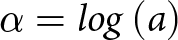 $\alpha = log\left( a \right)$
In this framework, b serves as the allometric exponent; b = 3 represents isometric growth, whereas deviations from this value indicate either negative or positive allometric shifts.
Model specification and hierarchy
To evaluate how model architecture influences biological inference and predictive performance, we contrasted four distinct Bayesian model families. Model M1 provided a sex-agnostic baseline, assuming a uniform relationship under a Gaussian error distribution:
 \begin{equation*}log\left( {W_i} \right) \sim \mathcal{N} \left( \alpha +blog\left( C{W_i} \right),\sigma \right)\end{equation*}
Model M2 tests whether sexes differ in baseline mass and in the allometric slope by adding a sex main effect and a sex × size interaction, allowing both the intercept and the CW–W trajectory to vary by sex:
 \begin{equation*}log\left( {W_i} \right) \sim \mathcal{N} \left( \alpha +blog\left( C{W_i} \right)+\gamma Se{x_i}+\delta log\left( C{W_i} \right)\times Se{x_i},\sigma \right)\end{equation*}
Crustacean morphometric datasets may contain outlying observations that are not well handled by a Gaussian likelihood. We therefore specified Model M3 with Student’s t-errors, where the degrees-of-freedom parameter (ν) controls tail heaviness. We also centred the log-width predictor ( $clog\left( C{W_i} \right) = log\left( C{W_i} \right)-\overline{log\left( CW \right)}$) so that the intercept corresponds to the expected log-weight at an average-sized crab, improving interpretability and helping stabilize sampling.
 \begin{equation*}log\left( {W_i} \right) \sim {t_\nu}\left( \alpha +bclog\left( C{W_i} \right)+\gamma Se{x_i}+\delta clog\left( C{W_i} \right)\times Se{x_i},\sigma \right)\end{equation*}
Model M4 explored a partial pooling alternative, assuming a shared allometric slope across sexes while permitting sex-specific offsets in baseline mass through a random intercept:
 \begin{equation*}log\left( {W_i} \right) \sim {t_\nu}\left( \alpha +bclog\left( C{W_i} \right)+{u_{Sex\left( i \right)}},\sigma \right),{u_{Sex}} \sim \mathcal{N} \left( 0,\tau \right)\end{equation*}
In Models M2 and M3, sex effects were treated as fixed interactions because the grouping variable contains only two levels. With such a limited number of groups, random-effects structures are frequently prone to weak identification and singular fits (Gelman and Hill, Reference Gelman and Hill2006; Barr, Reference Barr2013). Thus, the random-intercept in M4 was included primarily as a principled comparator to evaluate the efficacy of partial pooling for capturing level differences.
Prior distributions
Our choice of priors was informed by regional and species-specific literature indicating that b commonly falls around 2.8–3.1 and that a on the mm–g scale typically lies between 10−4 and 10−3 (Atar and Seçer, Reference Atar and Seçer2003; Gökçe et al., Reference Gökçe, Ergüden, Sangün, Çekiç and Alagöz2006; Sümer et al., Reference Sümer, Teksam, Karataş, Beyhan and Aydın2013; Rady et al., Reference Rady, Sallam, Abdou and El-Sayed2018; Palomares and Pauly, Reference Palomares and Pauly2025). Weakly informative priors were adopted, with all logarithms treated as natural logs.
For M1 and M2, the intercept α = log(a) utilized a Normal (−8.5, 1.02) prior, and the slope b utilized Normal (3.0, 0.252). Additional fixed effects in M2 were assigned weak Normal (0, 1) priors. For M3 and M4 (using the centred predictor), the intercept used Normal (5, 1.52) and the slope used Normal (3.0, 0.252). The residual scale σ followed a Student’s t (3, 0, 1) distribution. In M4, the group-level standard deviation was set to Student’s t (3, 0, 0.3); where a random slope + intercept structure was required, an LKJ(4) prior was specified for the correlation components.
Bayesian estimation, diagnostics, and posterior predictive checks
All Bayesian models were fitted in R using four Markov chains (4,000 iterations each; 1,000 warm-up). For the Hamiltonian Monte Carlo sampler, we used adapt_delta = 0.99–0.999 and max_treedepth = 15, with stricter settings applied to the robust specifications. Convergence was assessed using  $\hat R$ (values near 1.0) and effective sample size. When divergent transitions occurred, we addressed them primarily through predictor centring and, where needed, modest simplification of the parameterization.
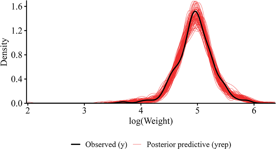
Model adequacy was assessed via posterior predictive checks by comparing the observed log-weight distribution (y = log(W)) to simulated replicates using density overlays. We additionally plotted the median fitted relationship and 90% uncertainty bands (backtransformed to grams) over the raw observations to detect systematic lack of fit.
Model comparison and selection
Candidate models (M1–M4) were compared using PSIS-LOO (Pareto-smoothed importance sampling leave-one-out) cross-validation (Vehtari et al., Reference Vehtari, Gelman and Gabry2017). For each model, we computed the elpdloo (expected log predictive density) and its standard error (SE), while inspecting observation-level Pareto-k diagnostics for reliability. Selection was primarily based on elpdloo values, supported by posterior predictive performance. Additional criteria included the residual scale (σ) and – where interactions were present – whether the 95% credible interval (CrI) for the sex-specific slope difference excluded zero.
Software
All analyses were conducted in R (R Core Team, 2024). Data handling and visualization relied on tidyverse (Wickham et al., Reference Wickham, Averick, Bryan, Chang, McGowan, François, Grolemund, Hayes, Henry, Hester, Kuhn, Pedersen, Miller, Bache, Müller, Ooms, Robinson, Seidel, Spinu, Takahashi, Vaughan, Wilke, Woo and Yutani2019) and tibble (Müller & Wickham, Reference Müller and Wickham2023). Bayesian modelling used brms (Bürkner, Reference Bürkner2017, Reference Bürkner2018, Reference Bürkner2021) with rstan (Stan Development Team, 2025). Posterior summaries used posterior (Bürkner et al., Reference Bürkner, Gabry, Kay and Vehtari2025). Model comparison used loo (Vehtari et al., Reference Vehtari, Gelman and Gabry2017, Reference Vehtari, Gabry, Magnusson, Yao, Bürkner, Paananen and Gelman2024; Yao et al., Reference Yao, Vehtari, Simpson and Gelman2018). Plot annotation used glue (Hester and Bryan, Reference Hester and Bryan2024). The study-area map was produced in R with sf (Pebesma, Reference Pebesma2018), ggplot2 (Wickham, Reference Wickham2016), rnaturalearth (Massicotte and South, Reference Massicotte and South2026) using the rnaturalearthdata (South et al., Reference South, Schramm and Massicotte2024) and rnaturalearthhires (South et al., Reference South, Schramm and Massicotte2025) basemaps, ggspatial (Dunnington, Reference Dunnington2025), and cowplot (Wilke, 2025); all figures were exported with ragg (Pedersen and Shemanarev, Reference Pedersen and Shemanarev2025).
Results
Morphometric characterization
A total of 197 individuals (C. sapidus) were used for analysis. CW values ranged from 81 to 195 mm, with a mean of 138.6 mm (±1.14 mm) and a median of 140.0 mm. The CW distribution was balanced, with individuals mostly clustered between 130 and 148 mm (interquartile range [IQR] = 18 mm). W ranged from 39.8 to 357.6 g, with a mean of 149.9 g (± 3.41 g) and a median of 142.1 g. The mean was higher than the median value, particularly due to the influence of large individuals above 175 g. This indicated a clear right skew in the data. Of the 197 specimens retained for analysis, 31 were males and 166 were females, giving a strongly female-biased sex ratio (≈5.4: 1) that reflects the composition of trap catches during the warm season. CW width ranged from 109 to 172 mm in males (mean 138.0 mm) and from 81 to 195 mm in females (mean 138.8 mm). The female size composition was strongly concentrated in the upper part of this range: 73.5% of the females measured between 130 and 160 mm CW (IQR = 130–148 mm) and were therefore predominantly adults, whereas individuals below 110 mm CW made up only 3.0% (n = 5) of the female sample. The imbalanced sex ratio, and in particular the small number of males (n = 31), should be borne in mind when interpreting the wider credible intervals obtained for the male scaling parameters. The strong positive relationship between CW and W was identified through preliminary visual inspection, and allometric scaled models were applied.
Classical allometric fit (OLS)
Standard OLS regression on log-transformed data explained approximately 70% of the observed variance (R 2 = 0.70, p < 0.001). The estimated allometric exponent (sexes combined) was b = 2.22 (SE = 0.10, 95% confidence interval (CI): 2.01–2.41), while the scaling coefficient was a = 0.00268. Given that the 95% CIfor b remained entirely below the isometric threshold of 3.0, the OLS model indicates significant negative allometric growth, suggesting that weight increases more slowly relative to CWs.
Bayesian model comparisons and selection
The sex-agnostic Gaussian model (M1), fitted to both sexes pooled, yielded an exponent b = 2.32 (95% CrI: 2.14–2.51), which was quantitatively consistent with the OLS estimates and further supported the negative allometry hypothesis. However, the introduction of sex-specific parameters in Model M2 revealed divergent scaling patterns. In this Gaussian interaction model, the male slope was estimated at b M = 2.50 (95% CrI: 2.25–2.75), whereas the female slope was lower, with a posterior difference (Δb F − M) of − 0.26 (95% CrI: −0.53 to 0.00).
The robust Student’s t model with a centred predictor (M3) provided the most comprehensive fit to the data. M3 estimated a male slope of b M = 2.70 (95% CrI: 2.40–3.00) and a substantial female-to-male slope difference of −0.52 (95% CrI: −0.87 to −0.17), implying a female exponent of bF ≈ 2.18. The residual scale was notably reduced (σ = 0.12), and the degrees of freedom parameter (ν = 8.0) confirmed the presence of heavy-tailed residual behaviour, justifying the shift from Gaussian to Student’s t-errors. Model adequacy for M3 was confirmed via posterior predictive checks, which demonstrated a high degree of overlap between the observed data and the model’s simulated replicates (Figure 2).
Posterior predictive check for the selected robust Student’s t interaction model (M3).

While the random-intercept model (M4) also demonstrated strong predictive performance, it was inherently more restrictive as it only permitted level shifts through partial pooling without directly parameterizing slope differences. PSIS-LOO cross-validation identified M3 as the superior model, characterized by the highest predictive density (elpd_loo = 101.11) and the highest precision. Crucially, as shown in Table 1, the 95% CrI for the slope difference in M3 did not overlap with zero, providing definitive evidence for sex-specific scaling.
Comparative summary of Bayesian model parameters and predictive performance

Table 1 Long description
Four models labeled M1 through M4 are compared across columns for sigma with credible interval, nu with credible interval, slope differences F to M credible interval, elpd loo, and elpd se. M1 reports sigma 0.17 with credible interval 0.158 to 0.193, no nu value, no slope differences value, elpd loo 64.21191, and elpd se 9.916032. M2 reports sigma 0.15 with credible interval 0.13 to 0.16, no nu value, slope differences minus 0.26 with credible interval minus 0.53 to 0.00, elpd loo 97.34773, and elpd se 12.696214. M3 reports sigma 0.12 with credible interval 0.10 to 0.14, nu 8.0 with credible interval 2.75 to 25.6, slope differences minus 0.52 with credible interval minus 0.87 to minus 0.17, elpd loo 101.11194, and elpd se 13.275236. M4 reports sigma 0.13 with credible interval 0.10 to 0.15, nu 11.16 with credible interval shown as 3.1635.46, no slope differences value, elpd loo 100.30844, and elpd se 12.595327.
Final parameter estimates
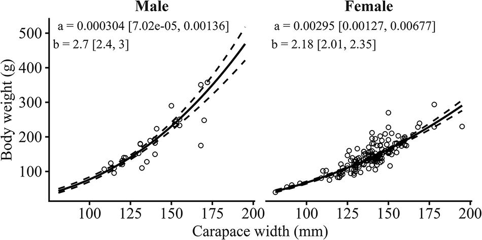
Based on the selected model (M3), the back-transformed parameters confirm negative allometric growth for both sexes, though the magnitude differs significantly. For males, the scaling was a M = 3.04 × 10⁻⁴ with an exponent b M = 2.70. For females, the scaling was a F = 2.95 × 10⁻³ with a notably shallower exponent b F = 2.18. As illustrated in Figure 3, these results indicate that while weight increases with CW in both sexes, males exhibit a significantly steeper growth trajectory compared to females.
Allometric relationship between carapace width (CW) and total weight (W) for male and female Callinectes sapidus.

Discussion
Relationships between weight and length are generally interpreted as simple estimates based on simple parameters a and b. However, the assumptions underlying the analyses used significantly affect the results. As with most species, sex-related differences in blue crabs may affect relationship estimates due to outliers arising from moulting, feeding, and reproductive activities. This situation may prevent adequate explanation using a Gaussian distribution.
Among the model comparisons made in this study, the model that best interpreted the data was the sex-specific robust Student’s t-distribution (M3). The results also support reporting uncertainty explicitly without relying only on back-transformed point estimates, consistent with recommendations in ecological modelling (Gelman and Hill, Reference Gelman and Hill2006; Barr, Reference Barr2013).
In our analysis, Model M4 illustrates that partial pooling can help stabilize estimates. However, with a simple grouping structure (two sexes), it does not replace a direct test of slope differences, which is provided by the interaction terms in M3. Given that random-effects structures can be weakly identified when a grouping factor has very few levels, we used fixed interactions to evaluate sex-specific scaling.
In all the models created, exponent (b) was observed to be below 3. This indicates the presence of negative allometry. It is known that the departure from isometric growth in decapod species is generally associated with shifts in energy transfer due to ontogenetic morphological changes (Hartnoll, Reference Hartnoll1978, Reference Hartnoll and Bliss1982).
Our sampling focused on the warm season (between June and October), when Mediterranean blue crabs are frequently reported to concentrate in shallow transitional waters such as the estuarine corridor of Azmak Stream (Ağbaş, Reference Ağbaş2006; Sümer et al., Reference Sümer, Teksam, Karataş, Beyhan and Aydın2013; Mancinelli et al., Reference Mancinelli, Chainho, Cilenti, Falco, Kapiris, Katselis and Ribeiro2017; Rady et al., Reference Rady, Sallam, Abdou and El-Sayed2018). During this period, C. sapidus individuals are engaged in reproductive activities, so individuals with different body weights can be observed within the same CWs. Additionally, the variation in moulting periods among individuals is a factor that can alter their weights. The sex-dependent growth trend observed in M3, which performed best in the established models, is consistent with the literature. In crustaceans, it is known that growth rates differ between sexes due to the development of secondary sexual characteristics and different reproductive requirements (Hartnoll, Reference Hartnoll1974, Reference Hartnoll and Bliss1982). Male C. sapidus individuals prioritize the development of a more advanced claw structure and muscle tissue production. This leads to an increase in their weight. Females, on the other hand, often expend their energy on gonad formation. For this reason, their length and body weight may not increase in a continuous linear fashion (Josileen, Reference Josileen2011). Consequently, the allometric exponent differs between males and females due to their use of energy for different purposes.
The unusually low female exponent (b F ≈ 2.18) is best understood in light of the terminal (pubertal) moult of female C. sapidus. Once females reach maturity, they undergo a final moult, after which CW remains essentially fixed while body mass continues to vary with ovarian maturation and nutritional condition. Our size composition shows exactly this situation. As reported above and illustrated in Figure 3, 73.5% of the sampled females measured between 130 and 160 mm CW and were predominantly adults, so the female dataset is dominated by individuals that had already completed the terminal moult. Following this moult, female energy allocation shifts away from somatic growth and is redirected towards ovarian maturation and reproductive output; body weight can therefore continue to increase substantially while CW no longer changes. Because sampling was confined to a specific temporal window (June–October), females were likely captured at various, non-synchronized stages of ovarian development, which further contributes to the high variance in body weight observed within a comparatively narrow range of CWs. This variance is not attributable to egg clutches: ovigerous females were released alive without being measured and are not part of the biometric dataset, so the scatter we observe reflects differences in the degree of ovarian development, feeding history, and moult condition among non-ovigerous adult females rather than the added mass of an external egg mass. Taken together, these processes decouple weight from width in adult females and drive the exponent well below isometry. Males, by contrast, continue to moult and grow after maturity, so that energy is still directed to overall somatic growth – including muscle mass and the enlargement of the chelae and other secondary sexual characters (Hartnoll, Reference Hartnoll1974, Reference Hartnoll and Bliss1982) – and weight therefore keeps tracking width more steeply. This heavy-tailed structure is not merely a statistical device; it captures the reproductively driven weight variation that a Gaussian likelihood would otherwise treat as lack of fit.
Regional studies from the Turkish coastline report strong CW–W relationships and repeatedly note sex-related differences in morphometrics (Atar and Seçer, Reference Atar and Seçer2003; Gökçe et al., Reference Gökçe, Ergüden, Sangün, Çekiç and Alagöz2006; Sümer et al., Reference Sümer, Teksam, Karataş, Beyhan and Aydın2013). Similar patterns occur elsewhere in the Mediterranean. In the northern Aegean, Kevrekidis (Reference Kevrekidis2019) reported negative allometry in females, with males closer to isometry and generally heavier at comparable widths. Comparable sex effects have also been reported from north-western (NW) Aegean Greece (Kampouris et al., Reference Kampouris, Kouroupakis and Batjakas2020) and northern Tunisia (Fassatoui et al., Reference Fassatoui, Hatira and Romdhane2021), indicating that Mediterranean populations may not follow a single, invariant scaling exponent. Importantly, these Mediterranean estimates were obtained under contrasting sampling regimes. Kevrekidis (Reference Kevrekidis2019) and Kampouris et al. (Reference Kampouris, Kouroupakis and Batjakas2020) sampled across broader seasonal windows in the northern and NW Aegean, whereas Fassatoui et al. (Reference Fassatoui, Hatira and Romdhane2021) reported a preliminary warm-period dataset from northern Tunisia; our own June–October coverage overlaps the reproductive and moulting season, when female weight is most variable. This methodological heterogeneity, rather than genuine biological divergence alone, likely contributes to the spread of published exponents. For juvenile stages, Gavioli et al. (Reference Gavioli, Mancinelli, Lanzoni, Franzoi, Moroni, Cardi, Eggleston, Christian and Castaldelli2026) linked CW–W condition to environmental drivers in the northern Adriatic, underscoring that ontogenetic stage and habitat further modulate the relationship. In the species’ native range, comparably low female exponents and sex-specific scaling have long been documented for Chesapeake Bay populations (Newcombe et al., Reference Newcombe, Sandoz and Rogers-Talbert1949), indicating that the divergence we report is an intrinsic feature of C. sapidus biology and not an artefact of its invasive Mediterranean populations.
For comparability across studies, CW–W relationships are usually reported in the power form W = aCWb. In this formulation, b captures allometric scaling and is commonly estimated on the log–log scale (Le Cren, Reference Le Cren1951; Froese, Reference Froese2006). Results can also be presented on the original scale, but the log-linear model remains the standard basis for consistent parameter estimation and interpretation across regions and datasets.
Two limitations should be borne in mind when interpreting these results. First, the number of males available for analysis was low (n = 31) and strongly outnumbered by females (n = 166). Although the Bayesian framework propagates this imbalance directly into the width of the posterior credible intervals, so that the greater uncertainty attached to the male exponent is reported rather than concealed, a sample of this size is not sufficient for a definitive description of male allometric growth; the male parameters presented here should therefore be regarded as provisional until larger and more balanced male samples become available. Second, sampling was restricted to the warm season (June–October) and to a single estuarine site, so the estimates describe CW–W scaling for that period and locality rather than for the complete annual cycle. Extending sampling across all seasons, over a wider size range and with a more balanced sex composition is a priority for refining the sex-specific conversion parameters proposed below for management use.
These findings carry practical consequences for managing the blue crab as both a nuisance invader and an emerging fishery resource in the Mediterranean. Because males and females follow distinct scaling trajectories, a single pooled CW–W equation systematically biases biomass reconstructed from carapace-width frequencies: it overstates the weight of large females and understates that of large males. Where landings or removal programmes are quota-, size- or biomass-based, applying sex-specific parameters (a M = 3.04 × 10⁻⁴, b M = 2.70; a F = 2.95 × 10⁻³, b F = 2.18) will yield more defensible stock and yield estimates and, in turn, more credible cost–benefit assessments of control effort. Practically, minimum-landing-size and mesh regulations that ignore the earlier weight plateau of terminally moulted females may under-harvest reproductive females precisely when targeting them would most reduce recruitment. We therefore recommend that both suppression programmes aimed at limiting ecological and economic damage and any regulated commercial exploitation adopt sex-resolved morphometric conversions rather than uniform ones.
Acknowledgements
The authors used ChatGPT (OpenAI; accessed January 2026) solely for language editing and minor stylistic improvements. No AI tool was used for data analysis, interpretation, or generation of scientific content. The authors take full responsibility for the content of the manuscript.
Author contributions
T.C.: Formal analysis, Investigation, Methodology, Project administration, Visualization, Writing – review and editing. C.B.: Conceptualization, Data curation, Investigation, Resources, Writing – Original draft preparation. O.A.: Investigation, Writing – review and editing, Validation. A.U.: Investigation, Writing – review and editing, Validation. I.L.M.: Writing – review and editing, Validation. All authors contributed to the final versions.
Declaration of interest
The authors declare none.
Data availability statement
The data that support this study cannot be publicly shared due to ethical or privacy reasons and may be shared upon reasonable request to the corresponding author if appropriate.
Ethics and approach
Not applicable.
Funding statement
This work was supported by Ege University Scientific Research Projects Coordination Unit (Grant No. 29601).



 Open access

