3.1. Case $r_T=1$

When $r_T = 1$, the fundamental V1H1 seiche is directly forced and we obtain a resonant response. In the time series of interface height $h_i$ (figure 2a,b), we observe at position A (non-nodal for odd modes) that a wave response with the fundamental period develops, which corresponds to the occurrence of a basin-scale linear wave. As forcing continues, the fundamental response is subject to resonant amplification, and we observe an increase in the wave amplitude. The formation of nonlinear modes is highlighted at position B, which is nodal for odd-mode quasi-linear waves. There, a dominant wave response has a periodicity of half the fundamental period, which corresponds to the V1H2 mode. We observe that the growth of the amplitude of nonlinear waves is roughly ruled by the steepening time scale $T_s$; for $t>T_s$, the amplitude of nonlinear waves is nearly constant and high-frequency NLIWs develop. These waves can be observed as pulse-like waves that degenerate the large-scale waves marked with a circle in figure 2(a).

Figure 2.

(a,b) Time series of non-dimensional interface height $h_i/H$ for resonant forcing $r_T=1$ plotted versus the number of forcing periods at probes A and B, respectively. The signature of the high-frequency NLIWs is marked with a circle and the dashed grey vertical lines denote the non-dimensional time period $T_1/T_w$ and multiple values, while the dashed black vertical line denotes the non-dimensional steepening time scale. (c,d) Non-dimensional spectral energy of interface height (lines) and phase lag among isopycnals (grey crosses) at probes A and B, respectively. Vertical dotted lines represent non-dimensional forcing frequency and its $m$th superharmonics. 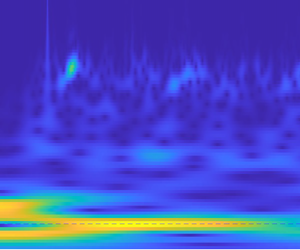Theoretical frequencies of internal seiches are integer values of $f/f_1$. (e,f) Wavelet spectra of interface height sampled at probes A and B, respectively. The dashed white horizontal lines denoted with letters indicate: $w$, forcing frequency $f_w$; f, fundamental frequency $f_1$; and $s$, approximate frequency of high-frequency NLIWs $\approx f_s$.

While we do not inspect the instantaneous fields for each high-frequency wave that appears in the time series, we note that the Richardson number $Ri$ (shown in § 4) is generally supercritical except in the near-surface layer; thus we can exclude shear instabilities as theorigin of these waves. The degeneration of the wave field by high-frequency NLIWs is expected based on Horn's diagram, and they are the only high-frequency waves that we observe in instantaneous fields. The high-frequency NLIWs propagate with almost permanent form, and therefore they can be observed at all locations. They decay in time due to viscous wall effects (Koop & Butler Reference Koop and Butler1981; Tang, Patel & Landweber Reference Tang, Patel and Landweber1990) or they deform and disintegrate (Grimshaw et al. Reference Grimshaw, Pelinovsky, Talipova and Kurkina2010). Given that our time series contain many superimposed waves, we cannot directly observe these changes.

The presence of higher horizontal modes is also evident in the energy spectrum of the interface height time series (figure 2c,d). We indicated forcing frequency $f_w$ and its superharmonics $f_{wm}=mf_w$, $m=2,3,\ldots$. The fundamental frequency of the basin-scale linear wave is $f_1$ and the higher-mode frequencies are calculated as $f_n = f_1 /n$. Most energy is confined in the first mode, although appreciable energy is transferred by nonlinear interactions to the second horizontal mode. The excitation of higher horizontal modes up to mode 10 is observable in the spectra. To get information on the vertical structure of the modes identified by energy spikes, we calculate the phase lag (coherence phase interpreted as a phase lag) between the heights of the isopycnals $\rho _0\pm 0.25\Delta \rho$. The phase lag is generally very small across all frequencies, indicating that isopycnals maintain approximately constant vertical separation distances so that the system response corresponds to the first vertical mode. The largest phase lag is found only in the middle of the basin (position B) near the fundamental frequency, corresponding to the periodic spreading and contraction of isopycnals at this location.

To better understand the development of the wave field in time, we use the wavelet analysis of the interface height time series (figure 2e,f). The cone of influence is plotted within the white dashed lines; it represents the border between data with accurate time–frequency representation and data in the shaded region where the accuracy of data is potentially influenced by edge effects. Initially, the fundamental mode is energized. After the first forcing cycle, the resonant response begins, which is characterized by the increase of energy in the fundamental mode (figure 2e). With time, energy is gradually transferred towards modes with higher frequencies, and high-frequency NLIWs (approximately denoted by the dashed line $s$ at a frequency that corresponds to short NLIWs observed in the time series for $r_T = 1$) can be observed in the wavelet spectrum of time series from probe B (figure 2f). After the third oscillatory cycle, a quasi-steady state is reached without further changes in energy distribution.

The dominant vertical modes of the internal waves can be identified by looking at the vertical profiles of the velocity components. The vertical profile of streamwise velocity allows identification of the dominant mode; the vertical profile of vertical velocity, which is more sensitive to particular waves passing through the chosen location, helps identification of other higher vertical modes.

In figure 3 we show the vertical profiles of the spanwise-averaged velocity components at probe B at several phases during the oscillatory cycle. We observe the presence of a three-layer structure: the near-surface layer, where stratification is weak, which is characterized by high velocity gradient and a velocity that decreases rapidly up to the beginning of the strongly stratified region; a stratified middle layer, where the velocity decreases with lower shear; and the third layer in the lower unstratified region, where velocity is nearly uniform and changes sign, due to the inversion of the mean current. Overall, the behaviour is that of a two-layer response showing the presence of an upper layer moving along the wind direction and a lower layer moving in the opposite direction. This scenario corresponds to the first vertical mode V1, as described by Monismith (Reference Monismith1985) for a system exposed to surface forcing. Two local maxima of $\langle N^2 \rangle = -(g/\rho _0) \langle \partial \rho / \partial z\rangle$ form at $\varphi =0$ and ${\rm \pi}$ and they collapse to a single one at $\varphi =0.5{\rm \pi}$ and $1.5{\rm \pi}$, indicating that these variations of density profile are not permanent.

Figure 3.

Vertical profiles at probe B of (a) $\langle u \rangle / u_*$, (b) $\langle w \rangle / u_*$ and (c) $\langle N^2 \rangle$. Curves: ——, $\varphi =0$; $\cdot \cdot \cdot \cdot \cdot$, $\varphi =0.5{\rm \pi}$; – – – –, $\varphi ={\rm \pi}$; and – $\cdot$ –, $\varphi =1.5{\rm \pi}$. The initial position of the middle layer is between $z/H = 0.7$ and $z/H = 0.9$.

During the resonant two-layer response, the maximum streamwise velocity of the metalimnion is ${\approx }5u_*$, and it reduces to ${\approx }2u_*$ in the hypolimnion. Surface velocity locally reaches values of $20u_*$. The near-surface region follows the forcing oscillatory behaviour with a phase lag between streamwise velocity $u$ and forcing $\tau$ of about $\Delta \varphi \approx 0.2{\rm \pi}$.

As observed by Lorke et al. (Reference Lorke, Umlauf, Jonas and Wüest2002), under the influence of seiching, the bottom boundary layer dynamics are governed by the oscillatory nature of the system. In our case, the bottom boundary layer is periodically driven by the internal seiches, as a system response to wind forcing; hence we use a simple analysis for Stokes oscillatory bottom boundary layer (SBL).

The Reynolds number, based on the Stokes viscous penetration length $\delta _S=\sqrt {2\nu /(2{\rm \pi} f_w)}$, is $Re_\delta =U_0 \delta _S/\nu$. As free-stream velocity, we use the maximum velocity of the bottom layer and obtain $Re_\delta = 44.5$, which is strictly in the laminar regime – for details see Salon, Armenio & Crise (Reference Salon, Armenio and Crise2007) and references therein. Consistently, we do not observe any indicators of turbulent disturbances. In other words, in the present case the bottom boundary layer generated by the internal seiches is weak and not able to produce substantial turbulence in the hypolimnion. The SBL behaviour matches that observed by Lorke et al. (Reference Lorke, Umlauf, Jonas and Wüest2002) when analysing field data, although in our study a scale effect on Reynolds number is present. Ulloa et al. (Reference Ulloa, Constantinescu, Chang, Horna-Munoz, Steiner, Bouffard and Wüest2019) found a large value of the turbulent intensity parameter in a region near the centre of the basin in their real-scale simulation.

3.2. Case $r_T=2$

Variation of the forcing period dramatically changes the response of the basin. The time series of the interface height for the forcing period $r_T=2$ is plotted in figure 4(a,b). After the initial fundamental wave response, characterized by a linear wave with the fundamental period (marked with the grey dashed vertical lines), the oscillation adjusts to the forcing period together with the appearance of high-frequency waves. Based on the analysis of Boegman et al. (Reference Boegman, Imberger, Ivey and Antenucci2003) for high-frequency waves, these waves are excited by nonlinear effects and we denote them as high-frequency NLIWs. They cannot be associated with shear instability because they occur in a region where the Richardson number $Ri=\langle N^2\rangle /\langle S^2\rangle$ is well above the critical value $Ri_{cr}=0.25$ under which shear instability can develop. The nonlinear effects that excite high-frequency NLIWs, in this case, are related to the destruction of the fundamental wave. Their presence just at probe A together with an inspection of the instantaneous field suggests that they are created locally, between probe A and the left endwall, and they travel towards the left endwall, where they lose a substantial part of their energy.

Figure 4.

(a,b) Time series of non-dimensional interface height $h_i/H$ for $r_T=2$ plotted versus the number of forcing periods at probes A and B, respectively. The dashed grey vertical lines denote the non-dimensional time period $T_1/T_w$ and multiple values, while the dashed black vertical line denotes the non-dimensional steepening time scale. The arrow denotes the fundamental wave destruction event. (c,d) Non-dimensional spectral energy of interface height (lines) and phase lag among isopycnals (grey crosses) at probes A and B, respectively. Vertical dotted lines represent forcing frequency and its $m$th superharmonics. Theoretical frequencies of internal seiches are integer values of $f/f_1$. (e,f) Wavelet spectra of interface height sampled at probes A and B, respectively. The dashed white horizontal lines denoted with letters indicate: $w$, forcing frequency $f_w$; f, fundamental frequency $f_1$; and $s$, approximate frequency of high-frequency NLIWs $\approx f_s$.

According to Cooker, Weidman & Bale (Reference Cooker, Weidman and Bale1997) upon collision of a large-amplitude solitary wave with a vertical wall, it loses energy (to a dispersive wave train) and height, which explains why we do not observe these high-amplitude, high-frequency NLIWs later in the time series. Instead, high-frequency waves with lower amplitudes appear and remain present throughout the simulation. Given that the Richardson number is very high in the metalimnion, all of these high-frequency waves are NLIWs. At the nodal location B, the initial response corresponds to even mode V1H2 with frequency $f_2$. However, as the system basin-scale response adjusts to the forcing conditions, due to energy transfer, so do the higher modes, as the period of the second horizontal mode at location B adjusts to the half-period of forcing $f_{w2}$. In this case, we do not observe resonant amplification.

In spectral energy analysis of these time series (figure 4c,d), we can identify forcing frequency $f_w$ as the most energetic at location A. The energy spike that belongs to the fundamental wave V1H1 is found near $f_1$ at the same location. At location B, which is nodal for the fundamental wave, the spike of energy near $f_1$ is associated with a wave that occurs as a superharmonic of the forcing frequency near $f_1 = f_{w2}$. Higher superharmonics of the forcing frequency can be identified: $f_{w3}$ at non-nodal location A; and $f_{w4}$ and $f_{w5}$ at nodal position B. The phase lag near $f_w$ and $f_{w4}$ indicates that these waves are in the form of higher vertical modes. There is increased energy in the region with high-frequency NLIWs (circled), which is characterized by the absence of a phase lag, indicating the presence of V1 mode.

The wavelet spectrum analysis of interface height series (figure 4e,f) shows that, initially, both the fundamental frequency and the forcing frequency are energized. During the second forcing period, the energy of the fundamental wave mode decreases rapidly (figure 4e), followed by the transfer of energy to nonlinear waves (figure 4f) and towards the high-frequency NLIWs. Upon transfer, energy is soon dispersed. After the decay of the fundamental mode, the energy of the wave with the frequency of forcing $f_w$ rises. Part of this energy is transferred to higher modes $f_{wm}$ up to the high-frequency NLIWs that develop as a result of steepening of the nonlinear waves.

Antenucci, Imberger & Saggio (Reference Antenucci, Imberger and Saggio2000) analysed data from field observations using an analytical model and found that a forcing period equal to that of the internal wave is not enough for resonant amplification. If the wave is pre-existing, the phase between wind and wave plays an important role. A zero phase causes resonant amplification, while a phase equal to $180^\circ$ (half-period) causes antiresonance and wave cancellation. Vidal et al. (Reference Vidal, Rueda and Casamitjana2007) further hypothesized that strong wind events that are out of phase with the dominant wave drain its energy and energize other vertical modes. Observing the destruction event on figure 4(a) (marked with an arrow), we see that the existing wave reaches its peak amplitude when forcing is at phase $\varphi = 0$, yielding a phase difference between wave and forcing of about a quarter of the forcing period. This difference is enough to drain energy from the fundamental mode and cause a wave cancellation. This process occurs with energy transfer from a quasi-linear fundamental wave to NLIWs, and subsequent energizing of the non-resonant wave with frequency $f_w$ and higher vertical mode.

The behaviour of the velocity and density fields during the wave cancellation events is depicted in figure 5. At $t/T_w = 0.7$ the wave starts its upward motion on the left side of the basin, which can be observed in the time series sampled at location A, and develops positive streamwise velocity $u$ in the middle layer, while the forcing produces negative $u$ near the surface, which is in the same direction as the flow in the bottom layer. At $t/T_w = 0.9$ to $t/T_w = 1$, the velocity in the middle layer intensifies, and spread and contraction of the metalimnion occur, respectively, at the left and at the right endwall. At $t/T_w=1$ the basin-scale V1 wave is at its own peak and about to start the downward motion (at the left side, where the sampling point is) and to reverse its circulation. At $t/T_w = 1.1$ close to the bottom and endwalls, $u$ has reversed its direction, while most of the middle and upper layer are still strongly dominated with the forcing-induced velocities from the previous forcing period. At the left side of the basin, where the metalimnion is contracted, short waves appear whose signature in $u$ is visible throughout the upper part of the water column. At $t/T_w = 1.2$ both density and velocity field are favourable for the formation of V2 waves.

Figure 5.

Illustration of the velocity and density fields during the wave cancellation event. Time series display the oscillation of isopycnal $\rho _0$ at $0.25L$ while red areas display the state of the non-dimensional forcing $\tau /u_*^2$. The five panels above the time series show internal fields at various times. White lines show the isopycnals in the range $\rho _0\pm 0.5\Delta \rho$, arrows show velocity direction and the field is coloured with non-dimensional streamwise velocity $u/u_*$.

The increase of the period of oscillation substantially changes the response of the basin; namely, it moves from two-layer to three-layer dynamics. Vertical profiles of the averaged velocity components and squared buoyancy frequency at probe B are shown in figure 6 at different phases during the oscillatory cycle. A clear three-layer response is depicted with two horizontal velocity inversions at the edges of the metalimnion. Basically, in the surface and bottom layers, the flow moves in the same direction, and inversion is present in the intermediate stratified region. This comes from a combination of a spatially evolving wave (typical of oscillatory flows) and the inversion required by mass conservation due to the presence of the endwalls. This structure clearly indicates that the dominant response of the system is in terms of second vertical mode V2 with forcing frequency.

Figure 6.

Vertical profiles at probe B of (a) $\langle u \rangle / u_*$, (b) $\langle w \rangle / u_*$ and (c) $\langle N^2 \rangle$. Curves: ——-, $\varphi =0$; $\cdot \cdot \cdot \cdot \cdot$, $\varphi =0.5{\rm \pi}$; – – – –, $\varphi ={\rm \pi}$; and – $\cdot$ –, $\varphi =1.5{\rm \pi}$.

The maximum of the streamwise velocity in the metalimnion and hypolimnion is about $3u_*$ and $0.4u_*$, respectively. Vertical velocity is more sensitive to the passage of different waves. Together with profiles with one vertical reversal (at $\varphi =0$ and $0.5{\rm \pi}$), which corresponds to the second vertical mode, we can observe a profile with no reversals (at $\varphi =0.5{\rm \pi}$), which corresponds to the passage of a wave with the first vertical mode. The system adjusts to the forcing period via a second vertical mode, while waves with the first vertical mode remain present. The profile of $\langle N^2 \rangle$ shows periodic behaviour, where $\langle N^2 \rangle$ increases at $\varphi = 0.5{\rm \pi}$ and $1.5{\rm \pi}$ and decreases at $\varphi = 0{\rm \pi}$ and $1{\rm \pi}$. The increase of $\langle N^2 \rangle$ corresponds to stronger stratification as a consequence of the contraction of metalimnion, while the decrease of $\langle N^2 \rangle$ corresponds to the metalimnion spread, which is a behaviour characteristic of waves with second vertical mode. In this case, the Reynolds number of the bottom SBL is $Re_\delta =12.6$ for which the flow is again in the strictly laminar regime.

3.3. Case $r_T=3$

A third forcing period was considered, resulting in the response of the interface height time series depicted in figure 7(a,b). At the non-nodal location A, we observe that the initial response is in terms of a non-resonant fundamental seiche (the fundamental period is marked by vertical dashed grey lines) as predicted for the two-layer system based on the results of Boegman & Ivey (Reference Boegman and Ivey2012). During the third forcing period, the fundamental wave degenerates, and NLIWs become dominant. We note that the fundamental wave is cancelled and re-formed several times. The first cancellation is observed at the beginning of the second forcing period, similarly to the $r_T=2$ case. A fundamental wave peak appears at forcing phase $\varphi =0$, which results in fundamental wave cancellation and formation of a new fundamental wave; the transition is always followed by energy transfer towards higher frequencies and the appearance of the high-frequency NLIWs. At the nodal location B, the initial response has a half-fundamental period, therefore corresponding to V1H2 mode. At the beginning of the second forcing period, even modes and NLIWs with a half-forcing oscillatory period appear, corresponding to forcing superharmonic $f_{w2}$. Growth of nonlinear waves and the appearance of NLIWs does not occur at $T_s$, so we can argue that their origin is related to processes that are not explained by the two-layer theory from which the steepening time scale $T_s$ is derived.

Figure 7.

(a,b) Time series of non-dimensional interface height $h_i/H$ for $r_T=3$ plotted versus the number of forcing periods at probes A and B, respectively. The dashed grey vertical lines denote the non-dimensional time period $T_1/T_w$ and multiple values, while the dashed black vertical line denotes the non-dimensional steepening time scale. (c,d) Non-dimensional spectral energy of interface height (lines) and phase lag among isopycnals (crosses) at probes A and B, respectively. Vertical dotted lines represent forcing frequency and its $m$th superharmonics. Theoretical frequencies of internal seiches are integer values of $f/f_1$. (e,f) Wavelet spectra of interface height sampled at probes A and B, respectively. The dashed white horizontal lines denoted with letters indicate: $w$, forcing frequency $f_w$; f, fundamental frequency $f_1$; and $s$, approximate frequency of high-frequency NLIWs $\approx f_s$.

We show the spectral energy of the interface height time series in figure 7(c,d). At non-nodal location A, the highest-energy peak is found at fundamental and forcing frequencies $f_1$ and $f_w$, respectively; at the nodal location B, the superharmonic $f_{w2}$ is even more energetic. At the non-nodal position, peaks of energy can also be observed for superharmonics $f_{w4}$ and $f_{w5}$ and at the nodal position for $f_{w4}$ and $f_{w6}$. Phase lag is generally high across most frequencies, indicating that the motion of isopycnals $\rho _0\pm 0.25\Delta \rho$ is practically decoupled and that the system responds with higher vertical mode. This is also true for the region with NLIWs.

The wavelet spectrum analysis of the interface height shown in figure 7(e,f) indicates that fundamental and forcing frequencies are dominant at probe A (figure 7e). The wave with fundamental frequency has a particular behaviour with respect to energy content, which is characterized by several events of increase and decrease of energy. These events coincide with the appearance of energy in the higher frequencies. The sudden losses in fundamental wave energy are caused by wave cancellation, due to the phase difference between wave and forcing. Besides the high-frequency NLIWs that originate from the wave cancellation events, there are energy bursts in NLIWs with lower frequencies whose energy increases with each occurrence, which will be discussed later. At location B (figure 7f), substantial energy is contained in the even superharmonic $f_{w2}$. In fact, energizing of $f_{w2}$ coincides with both energy loss from $f_w$ and cancellation of $f_1$, upon which the energy of $f_{w2}$ remains constant throughout the simulation. This leads to the conclusion that the system adjusts to the $f_{w2}$ response. Given that this wave is absent at location A, and this location is nodal for H2 waves, we can identify this wave as horizontal H2 mode. The wavelet spectrum analysis of the time record at probe B shows that superharmonics originate from $f_{w2}$. Besides, we see the pathways of energy towards high-frequency NLIWs, which occur with period $0.5T_w$ (corresponding to $f_{w2}$). By inspecting the spanwise-averaged fields at the time instant (discussed in the § 4), we find that these are V2 mode NLIWs that periodically pass through the probe with frequency  $f_{w2}$.

The vertical profiles of the spanwise-averaged velocity components are shown in figure 8. The streamwise velocity profile (figure 8a) has a three-layer structure similar to that of the $r_T=2$ case, but it is substantially less uniform across the metalimnion. This indicates that the second vertical mode V2 dominates in the presence of other superimposed waves. Occasionally, metalimnion jet-like behaviour appears, which is related to the V2 response. It reaches a velocity of about $4u_*$. By examining the instantaneous fields, we found that this behaviour is associated with the occurrence of V2 high-frequency NLIWs. Similar association of the V2 mode NLIWs with the metalimnic jet is made in Boegman et al. (Reference Boegman, Imberger, Ivey and Antenucci2003). Excluding the jet-like events, the maximum of the streamwise velocity in the middle layer is $\approx 2u_*$ and up to $\approx 0.4u_*$ in the lower layer. The vertical velocity profile (figure 8b) at $\varphi =0.5{\rm \pi}$ clearly belongs to the wave with the second vertical mode, while in other profiles different waves are superimposed. The metalimnion appears deepened compared to other cases (figure 8c), which is partially the consequence of substantially different duration of the numerical experiment. Even in this case ($Re_\delta =15.4$), the bottom layer flow is strictly in the laminar regime.

Figure 8.

Vertical profiles at probe B of (a) $\langle u \rangle / u_*$ (the inset shows the metalimnion jet at $\varphi =1.6{\rm \pi}$), (b) $\langle w \rangle / u_*$ and (c) $\langle N^2 \rangle$. Curves: ——-, $\varphi =0$; $\cdot \cdot \cdot \cdot \cdot$, $\varphi =0.5{\rm \pi}$; – – – –, $\varphi ={\rm \pi}$; and – $\cdot$ –, $\varphi =1.5{\rm \pi}$. As before, $\varphi$ indicates the phase within the forcing cycle.

Ulloa et al. (Reference Ulloa, Constantinescu, Chang, Horna-Munoz, Hames and Wüest2020) resonantly forced a nonlinear V2H1 wave that is characterized by a V2 undular bore and found that it is followed by a train of V2 high-frequency NLIWs. In our case, a nonlinear V2H2 wave is the dominant response, and its period corresponds to that of the passage of V2 NLIWs; therefore, V2H2 is likely to be the wave they originate from. The inspection of the structure of V2 NLIWs corresponds to the description of Ulloa et al. (Reference Ulloa, Constantinescu, Chang, Horna-Munoz, Hames and Wüest2020), where each wave consists of the two cores with opposite vorticity (not shown). While the association of the nonlinear V2 wave and V2 NLIWs corresponds to that observed by Ulloa et al. (Reference Ulloa, Constantinescu, Chang, Horna-Munoz, Hames and Wüest2020), the general response differs. Namely, we do not observe the differentiation on the quiescent and disturbed part of the domain by the nonlinear wave. This may be because in our case the nonlinear response is a non-resonant wave and there are a variety of other superimposed waves in the field.

3.4. Summary

In basins where metalimnion thickness cannot be neglected and when periodic forcing has period close to or greater than the fundamental one (which is the case for most small and mid-sized lakes), only resonant forcing of V1H1 ($r_T\approx 1$) excites a response in terms of first vertical mode. Forcing with larger forcing period produces a response with higher vertical mode; in the cases we tested, $r_T= 2,3$, the wave response has a second vertical mode. The excitation of the higher vertical modes by larger $r_T$ is expected because the propagation speed of vertical mode-$n$ waves decreases roughly like $n^{-1}$ (Monismith Reference Monismith1987), which increases the period of these waves with $n$. We may argue that the limit for resonant excitation of V1H1 is $r_T\gtrapprox 1.5$ as determined by Boegman & Ivey (Reference Boegman and Ivey2007) for a two-layer system. The results of Boegman & Ivey (Reference Boegman and Ivey2007) are also valid for the initial response for forcing periods larger than those given by the above condition, where the initial response is in terms of the non-resonant fundamental wave.

Differences arise after a time period when forcing conditions become unfavourable to the fundamental wave, and lead to its cancellation. This process results in transfer of energy from the fundamental mode to high-frequency NLIWs through nonlinear mechanisms. In the $r_T=2,3$ cases, the first cancellation occurs at about ${\approx }1.15T_w$. Upon cancellation, the wave field develops differently depending on the forcing period. Namely, for $r_T=2$, this cancellation is permanent; the system adjusts to forcing by energizing the V2H1 wave whose frequency corresponds to that of the forcing. For $r_T=3$, the fundamental wave V1H1 re-forms and gets cancelled several times during the oscillatory cycles. Upon the first cancellation, forcing superharmonic $f_{w2}$ is energized as nonlinear V2H2, while the energy of $f_w$ decreases; therefore, the system adjusts to nonlinear $f_{w2}$ and it becomes the dominant response.

Generalizing the results, a lake-like system with a fundamental period shorter than diurnal and having relatively thick metalimnion compared to other layers is susceptible to the formation of higher vertical modes and will respond with higher vertical mode waves unless the fundamental wave is resonantly forced with $r_T\lessapprox 1.5$. The response can adjust to forcing frequency $f_w$ or to its superharmonic. The ability of the system to adjust to the periodicity of the forcing is closely related to the occurrence of NLIWs, and they might be a bridge for internal adjustment.

4.1. Resonant response, $r_T=1$

The time series of interface height in figure 9(a,b) show that, as $\alpha$ decreases, high-frequency NLIWs (circled) appear before the steepening time scale $T_s$, indicating that the mechanism of their formation is not gradual energy transfer from quasi-linear waves to nonlinear ones and their subsequent steepening. As in the previous section, the presence of high-frequency NLIWs in the time series is characterized by high-frequency pulse-like waves superimposed on the main almost sinusoidal low-frequency wave field. Another effect of inclination of the endwall is that the time series are smoother, with less pronounced high-frequency NLIWs for small values of $\alpha$. The time series are all very similar apart from $\alpha \leq 45^\circ$, for which the amplitude of the oscillation of density interface reduces substantially with time at both probes. This matches the behaviour speculated by Ulloa et al. (Reference Ulloa, Constantinescu, Chang, Horna-Munoz, Hames and Wüest2020) that water bodies with a lower slope angle will escape resonance sooner than those with steep slopes due to enhanced mixing at the sloping boundaries which changes the background stratification. We will further discuss these effects later on.

Figure 9.

(a,b) Time series of interface height for $r_T=1$ and different values of $\alpha$ at probes A and B, respectively. (c–e) Vertical profiles of the velocity components and $\langle N^2 \rangle$ sampled at probe B for all values of $\alpha$. (f,g) Wavelet spectrum for $\alpha = 30^\circ$ at probes A and B, respectively. Dashed white horizontal lines denoted with letters indicate: $w$, forcing frequency $f_w$; f, fundamental frequency $f_1$; and $s$, approximate frequency of high-frequency NLIWs $\approx f_s$. (h,i) Slices through the instantaneous density field together with velocity vectors and interface $\rho =\rho _0$ denoted with a white line for the case $\alpha = 30^\circ$ at time instants $t/T_w = 0.9$ and $t/T_w = 1$, respectively. Colour code for (a–e): black, $\alpha =90^\circ$; red, $\alpha =75^\circ$; green, $\alpha =60^\circ$; blue, $\alpha =45^\circ$; and brown, $\alpha =30^\circ$.

The energy spectra of the time series of interface height are very similar for all inclination angles of the endwalls (not shown). Also, the phase lag between the two chosen isopycnals is generally low, except at frequencies near $f_1$ in the middle of the channel. This corresponds to periodic spread and contraction of the metalimnion in the middle of the basin, which is the indicator of the formation of higher vertical modes. This effect is more pronounced for the lower inclination of the endwalls.

The wavelet spectrum analysis of the time series for $\alpha = 30^\circ$ shown in figure  9(f,g) reveals that high-frequency NLIWs form before $T_s$, at the end of the first forcing period, which can be observed as an increased amount of energy near the dashed line $s$ (figure 9f). We note that, before reaching high-frequency waves, energy is transferred through the lower frequencies. The origin of these waves may be attributed to forcing-induced nonlinear surges, like those observed by Farmer (Reference Farmer1978), that quickly steepen, thus producing high-frequency NLIWs. This is confirmed by inspection of the instantaneous fields: figure 9$(h)$ shows the formation of the surge at the interface (denoted with a downward triangle), while figure 9$(i)$ shows the degeneration of the surge into the high-frequency NLIWs.

The energy contained in the region of the high-frequency NLIWs is relatively low until the third forcing period, which corresponds to the formation of solitary-like waves by nonlinear steepening (timed by $T_s$), after which their energy is reduced. This behaviour is significantly different from that of the rectangular case, where, for $t>T_s$, a quasi-steady state is reached. The cause of this behaviour will be discussed later in this section.

Vertical profiles of averaged streamwise and vertical velocity components and squared buoyancy frequency are shown in figure 9(c–e). The vertical profiles of buoyancy frequency squared (figure 9e) show that the epilimnion becomes more stratified for steeper slopes. Given that the initial state of the epilimnion is uniform density $\langle N^2\rangle =0$, this indicates that, as the slope steepens, there is more mixing in the upper layer. Going down, we observe that for steep slopes $\alpha =75^\circ,90^\circ$, the maximum of $\langle N^2\rangle$ (indicating pycnocline) is shifted downwards. Both these phenomena can be explained by vigorous corner flow at the downwind end that appears for steep slopes (such as that described by Monismith (Reference Monismith1986) and Stevens & Imberger (Reference Stevens and Imberger1996)). This flow cannot penetrate through the metalimnion, but it erodes it with time. At the bottom of the metalimnion, the stratified region, with non-zero $\langle N^2\rangle$, spreads downwards with a decrease of $\alpha$. Mixing under the metalimnion can be explained in relation to the reduction/decrease of the high-frequency NLIWs from the wave field (as observed in figure 9a,b,f,g), as a consequence of breaking of the NLIWs at the slopes, which is known to cause mixing in the lower layer (e.g. Michallet & Ivey Reference Michallet and Ivey1999). Widening of the metalimnion is known to promote the formation of higher vertical modes.

The vertical velocity profiles (figure 9d) do not exhibit reversals, indicating V1 as the dominant vertical mode for all endwall angles. However, as $\alpha$ decreases, a substantial reduction of the vertical velocity and additional spatial oscillations occur. The first one is explained by the resonance-escape hypothesis of Ulloa et al. (Reference Ulloa, Constantinescu, Chang, Horna-Munoz, Hames and Wüest2020), whereas the latter indicates the existence of higher vertical modes superimposed over the profile of the dominant V1H1 mode. The additional waves drain energy from the fundamental mode, causing the further reduction of the amplitude of vertical velocity, as observed in figure 9(d).

The vertical profile of streamwise velocity (figure 9c) changes little with the variation of the angle of the endwalls, and the behaviour roughly corresponds to that described for the rectangular domain. We observe that, as $\alpha$ decreases, the vertical profiles become less sharp, which is related to the appearance of higher vertical modes that create a non-uniform distribution of velocity in each layer.

The spatial oscillations observed in the vertical velocity profiles, together with the progressive irregularities of profiles of horizontal velocity component, for low endwall angles $\alpha$, indicate the increase of the number of shearing layers.

The quantity $\langle S^2\rangle =\langle \partial u/\partial z\rangle ^2+\langle \partial v/\partial z\rangle ^2$ is indicative of regions with high shear, where turbulence is more likely to occur if stratification is weak, resulting in low values of Richardson number. The largest values are close to the free surface in all cases, due to the action of the wind stress. The second region with high $\langle S^2\rangle$ is found in the lower end of the metalimnion where the velocity reverses (see figure 9c). Lowering of $\alpha$ introduces higher shear into the interior, as a direct consequence of the occurrence of the higher vertical modes. Indeed, they produce a number of layers moving with different velocities. In all cases, shear is evident close to the bottom, indicating the presence of a weak boundary layer, and at the inclined walls, for a low value of $\alpha$. As already discussed, the bottom boundary layer is very weak and in the laminar regime. This holds also in the presence of inclined walls.

The gradient Richardson number $Ri=\langle N^2\rangle /\langle S^2\rangle$ shown in figure 10 quantifies the relative importance of the local stabilizing buoyancy forces against the destabilizing effect of shear. In general, in our simulations, $Ri$ is very high, which is a consequence of the laboratory configuration. There is a thin near-surface layer where $Ri$ is under the critical value $Ri_{cr}=0.25$, which corresponds to the surface mixed layer, where $\langle N^2\rangle$ is very low and $\langle S^2\rangle$ is very high. This is the case also in real-scale basins. The region with subcritical and negative $Ri$ can be found near the corner due to the return jet, where the downward jet creates overturns. We observe that the downward reach of this jet increases with $\alpha$. In the interior, $Ri$ is generally supercritical; exceptions are the intermittent regions with subcritical $Ri$ that appear at the lower edge of the metalimnion (where $\langle N^2 \rangle$ is very low) for lower $\alpha$. For the lowest $\alpha$, some wider regions with $Ri< Ri_{cr}$ are observed, in particular near the walls, as a consequence of wave breaking, which will be discussed below in the following paragraphs. We acknowledge that, due to laboratory-type set-up, there is a lack of patches with subcritical $Ri$ that would produce shear instabilities and turbulence in the interior, compared to real lakes (Saggio & Imberger Reference Saggio and Imberger2001).

Figure 10.

Richardson number $Ri$ for $r_T=1$ at $\varphi =1.2{\rm \pi}$: (a)  $\alpha =90^\circ$, (b)  $\alpha =60^\circ$ and (c)  $\alpha =30^\circ$. The turquoise colour scale represents subcritical $Ri$.

In our numerical experiments, as in real lakes, the flow is strongly dominated by the internal wave field characterized by continuous variations in space and time, which produces high intermittency. In such situations, vertical fluxes (such as $\langle \rho ' w' \rangle$, $\langle u' w' \rangle$, …) appear at a similar rate as down-gradient and counter-gradient (Saggio & Imberger Reference Saggio and Imberger2001), indicating the presence of stirring, or reversible fluid rearrangement (see Linden Reference Linden2018; Villermaux Reference Villermaux2019; Caulfield Reference Caulfield2021). This characteristic of lakes makes it difficult to quantify the irreversible part of vertical density flux $\langle \rho ' w' \rangle$ and subsequently the buoyancy flux $B = (g/\rho_0)\langle\rho'w'\rangle$, which are needed in order to calculate the diffusivity of density $K_\rho = \langle \rho ' w' \rangle / (\partial \langle \rho \rangle / \partial z) = B/N^2$. The vertical fluxes are dominated by the reversible component in all simulated cases. In other words, these quantities are not very robust for quantification of mixing in the case studied herein.

There are several methods that have been developed in the literature to extract information on the turbulent mixing: the widely used Osborn–Cox method (Osborn & Cox Reference Osborn and Cox1972) evaluates the turbulent diffusivity of the scalar, using some assumptions that are difficult to verify in transitional non-equilibrium flows; the available potential energy methods (e.g. Winters et al. Reference Winters, Lombard, Riley and D'Asaro1995; Scotti & White Reference Scotti and White2014) directly relate changes in the available potential energy to irreversible diapycnal mixing; and, finally, there are parametrizations which constitute a simple and efficient way to obtain the desired field.

The laboratory-scale parametrization of $K_\rho$ for Prandtl number $Pr=0.7$ proposed by Shih et al. (Reference Shih, Koseff, Ivey and Ferziger2005) was extended to the range $0.7< Pr<700$ by Bouffard & Boegman (Reference Bouffard and Boegman2013). These models are based on the strong correlation between $K_\rho$ and the turbulence intensity parameter $Re_b=\epsilon /(\nu N^2)$, where $\epsilon$ is the dissipation rate of turbulent kinetic energy, namely, $K_\rho =C_1\nu Re_b^n$, where $C_1$ and $n$ are constants characteristic of the mixing regimes initially defined by Shih et al. (Reference Shih, Koseff, Ivey and Ferziger2005) and successively expanded by Bouffard & Boegman (Reference Bouffard and Boegman2013) as the molecular, buoyancy-controlled, transitional and energetic regimes.

We calculated the turbulence intensity parameter (or Reynolds buoyancy number) $Re_b$ using the dissipation rate $\epsilon = - (\nu + \langle \nu _{sgs} \rangle ) \langle ({\partial u''_i}/{\partial x_j})({\partial u''_i}/{\partial x_j})\rangle$, for $i,j=1,2,3$ and buoyancy frequency $\langle N^2 \rangle$.

Instantaneous resolved buoyancy fluxes in the metalimnion for the phase $\varphi =0.8{\rm \pi}$ are plotted as a function of the turbulence intensity parameter $Re_b=\epsilon /(\nu \langle N^2\rangle )$ in figure 11. Here we take the metalimnion to be the region $0.5< z/H<0.9$, which is wider than in the initial set-up, in order to account for metalimnion spread due to mixing (see figure 9e). We show the values of positive and negative buoyancy flux events as $B^+$ and $B^-$ made non-dimensional with $\kappa N^2$. We are not replacing $B/(\kappa N^2)$ with the equivalent expression $K_\rho /\kappa$ because the first contains events of reversible fluid rearrangement that do not contribute to turbulent mixing. We note that in our simulations the events with $Re_b$ values are significantly lower than in the real-scale simulations of Ulloa et al. (Reference Ulloa, Constantinescu, Chang, Horna-Munoz, Steiner, Bouffard and Wüest2019), where typical values of $Re_b$ in the metalimnion are ${\approx }10^2$ and at the sloped walls from about $10^2$ to $10^5$. Vertical lines divide different regions as defined by Bouffard & Boegman (Reference Bouffard and Boegman2013). Most of the distribution is found to be in the molecular and buoyancy-controlled regimes. This is due to the laboratory scale employed in our study, which is better suited for the analysis of internal wave dynamics rather than for the analysis of mixing. The values obtained in our simulations are higher than those estimated using the Bouffard & Boegman (Reference Bouffard and Boegman2013) parametrization for $Sc=500$, probably due to the reversible buoyancy fluxes associated with internal waves. The effect of the angle $\alpha$ is hardly detectable from these plots since the dots are overlapped over the same regions, but histograms (not shown) show the shift of the distribution towards higher values for lower $\alpha$.

Figure 11.

Non-dimensional buoyancy fluxes $B/(\kappa \langle N^2\rangle )$ as a function of turbulence intensity parameter $Re_b$ for $r_T=1$ at $\varphi =0.8$. Plots of directly calculated positive $B^+$ and negative $B^-$ buoyancy flux. Thick purple lines represent the parametrization of Bouffard & Boegman (Reference Bouffard and Boegman2013) for $Pr=500$ . Colour code: black, $\alpha =90^\circ$; red, $\alpha =75^\circ$; green, $\alpha =60^\circ$; blue, $\alpha =45^\circ$; and brown, $\alpha =30^\circ$.

Spatial distributions of the turbulent dissipation rate and turbulent diffusivity of density calculated using the Bouffard & Boegman (Reference Bouffard and Boegman2013) parametrization based on laboratory and numerical data are shown in figure 12. The turbulent dissipation rate $\epsilon$ (figure 12a–c) is larger near the surface and near the corner where vigorous corner flow is present. With the decrease of $\alpha$, we observe that the spatial distribution of dissipation rate changes substantially; regions with significant dissipation rate, which are in the path of the downward beams radiating off-slope, penetrate further into the hypolimnion; for the lowest values of $\alpha$, we find high dissipation rate in the regions where the metalimnion encounters the endwalls. For the lowest inclination angle, a large non-dimensional dissipation rate $\epsilon /(u_*^4/\nu )$ occurs in the metalimnion near the walls ${\sim }10^{-2} - 10^{-3}$, while in the interior it is ${\sim }10^{-5} - 10^{-6}$. This difference is close to that observed by MacIntyre et al. (Reference MacIntyre, Flynn, Jellison and Romero1999) for onshore and offshore dissipation rates (two to three orders of magnitude), while it is somewhat higher than that simulated by Ulloa et al. (Reference Ulloa, Constantinescu, Chang, Horna-Munoz, Steiner, Bouffard and Wüest2019) and substantially higher than that observed by Wain & Rehmann (Reference Wain and Rehmann2010).

Figure 12.

Fields of (a–c) non-dimensional turbulent dissipation rate $\epsilon /(u_*^4/\nu )$, (d–f)  dissipation rate of turbulent available potential energy $\epsilon _\rho /(u_*^2 N_{init})$ and (g–i)  turbulent diffusivity of density $K_\rho /\kappa$ for $r_T=1$ at $\varphi =0.4{\rm \pi}$ for (a,d,g)  $\alpha =90^\circ$, (b,e,h)  $\alpha =60^\circ$ and (c,f,i)  $\alpha =30^\circ$. White lines represent isopycnals. Closed yellow lines represent the unstable stratified regions with negative $\langle N^2 \rangle$.

We use the method of Scotti & White (Reference Scotti and White2014) in order to calculate the dissipation rate of the available potential energy $\epsilon _\rho$ as

(4.1)\begin{equation} \epsilon_\rho = \kappa \left\langle \frac{\partial\rho''}{\partial x_j}\frac{\partial\rho''}{\partial x_j} \right\rangle \frac{g^2}{2\rho_0^2 \langle N^2\rangle}, \end{equation}

which we show in figure 12(d–f). We note that the spatial distribution of $\epsilon _\rho$ is similar to that of $\epsilon$ with the abrupt drop in the hypolimnion region where $\langle N^2 \rangle\approx 0$. We note that, for the steep slopes $(\alpha = 60^\circ, 90^\circ )$, regions with high $\epsilon _\rho$ are located in the near-wall regions and upper metalimnion, while for the gentle slope $(\alpha = 30^\circ )$, high-$\epsilon _\rho$ regions are shifted towards the border between the metalimnion and unstratified hypolimnion.

We calculate the spatial distribution of diffusivity of density $K_\rho$ (figure 12g–i) and mixing efficiency $E$ (not shown) following VanDine, Pham & Sarkar (Reference VanDine, Pham and Sarkar2021), where $K_\rho = {\epsilon _\rho }/{\langle N^2\rangle }$ and $E = {\epsilon _\rho }/{(\epsilon +\epsilon _\rho )}$. We note that, for steep slopes, $K_\rho$ is high only near the surface and corner, where mixing is a direct consequence of forcing. As slope angle decreases, we observe some mixing also near the walls, at the edges of the metalimnion. The increase of mixing as the slope moves from steep to moderate, together with lowering of mixing location, corresponds to the behaviour associated with high-frequency NLIWs breaking (Michallet & Ivey Reference Michallet and Ivey1999; Boegman et al. Reference Boegman, Ivey and Imberger2005a) and shear-induced convective mixing (Lorke et al. Reference Lorke, Peeters and Wüest2005). For the lowest angle $\alpha = 30^\circ$, we observe an overturn event (region with negative $\langle N^2 \rangle$) at the bottom of the metalimnion.

The observed mixing efficiency is generally low throughout the metalimnion $(O(10^{-3}))$, while at the bottom of the metalimnion, where stratification is weak and shear is high due to the structure of the internal waves, $E$ is high locally $(O(10^{-2} - 10^{-1}))$ with highest values of almost  0.6.

We also observe downward beam-like activity near the sloped walls, and we investigate the criticality of the slopes. We use the slope criticality parameter (Garrett & Kunze Reference Garrett and Kunze2007; Gayen & Sarkar Reference Gayen and Sarkar2010, Reference Gayen and Sarkar2011) defined as $\gamma = {\tan \alpha }/{\tan \theta }$, where $\tan {\theta } = \sqrt {\omega _w^2/(\langle N^2 \rangle -\omega _w^2)}$ is the slope of the forced internal wave with frequency $\omega _w = 2{\rm \pi} f_w$. Slope criticality and observed beams are shown in figure 13. Slopes are near-critical at the bottom edge of the metalimnion (white line) and supercritical above it. In the streamwise velocity, we observe the downward beams that radiate away from the slopes, which is a known behaviour at supercritical slopes (Sarkar & Scotti Reference Sarkar and Scotti2017). These downward beams can induce turbulence and overturns on their path (Aucan et al. Reference Aucan, Merrifield, Luther and Flament2006). This explains the particular spatial distribution of $Ri$, where cases with low $\alpha$ show regions in the deep interior where the Richardson number is near-critical or subcritical. For $\alpha = 30^\circ$, there is a weak downslope flow near the critical region of the slope, which induces weak mixing ($K_\rho \approx 20\kappa$) at the endwalls and creates a region with subcritical $Ri$.

Figure 13.

Non-dimensional streamwise velocity component for $r_T = 1$ at $\varphi = 0$ for (a) $\alpha = 60^\circ$, (b) $\alpha = 45^\circ$ and (c) $\alpha = 30^\circ$. The line shows the slope criticality parameter $\gamma = 1$ and the arrows indicate the near-wall end of downward beams.

Near-shore mixing can be generated by seiching currents or breaking of internal waves. We observed in both time series and their wavelet spectrum analysis that high-frequency NLIWs are substantially reduced for low $\alpha$. In figure 14 we can observe the formation of an unstable layer during the upslope seiching event that corresponds to the shear-induced convective mixing as described by Lorke et al. (Reference Lorke, Peeters and Wüest2005). We can therefore conclude that the increased mixing and dissipation rate near the wall is due to the combination of wave breaking events and shear-induced mixing.

Figure 14.

Contours of density field and velocity direction for $\alpha =30^\circ$ at $\varphi = 1.8{\rm \pi}$, showing generation of unstable stratification during the upwelling event.

Time development of the horizontally (along $x$ and $y$ directions) averaged field $\langle N^2\rangle _h$ is shown in figure 15. In all cases, deepening of the metalimnion is more rapid during the initial transient, when shear-induced mixing occurs. According to Spigel & Imberger (Reference Spigel and Imberger1980), this mixing is later damped by the internal waves and the deepening slows down. There is a clear tendency of faster metalimnion deepening for basins with lower $\alpha$. It should be stressed that this deepening weakly stratifies the hypolimnion (which initially has uniform density) and it becomes susceptible to the occurrence of internal waves. On the other hand, deepening does not cause such dramatic changes in the stratified region, in terms of relocating isopycnals, as seen in figures 9(a,b) and 12.

Figure 15.

Time development of the horizontally averaged buoyancy frequency squared $\langle N^2\rangle _h$ for (a)  $\alpha =90^\circ$, (b)  $\alpha =60^\circ$ and (c)  $\alpha =30^\circ$.

Analysis of the time series, velocity, indicators of stratification and turbulence fields suggests the following scenario. After the initial transient, the mechanism that deepens the metalimnion for lower slope angles is a combination of wave breaking, seiching currents, downward beams and the presence of higher vertical modes. Owing to wave breaking, shear-induced mixing and near-critical or supercritical slopes, fluid under the metalimnion is getting mixed near the boundaries, whereas the higher vertical modes enhance the intrusion that transports this mixed fluid towards the interior (Wain & Rehmann Reference Wain and Rehmann2010).

4.2. Non-resonant response and wave destruction, $r_T=2$

In the interface height time series of figure 16(a,b), we observe similar oscillatory behaviour for cases with different angles of the endwalls. First, the fundamental mode is excited; later on, the forcing frequency dominates the oscillatory cycle. The inclination angle of the endwalls does not affect the response very much. For lower inclination angles, high-frequency waves appear earlier, being less pronounced in the later forcing periods compared to the rectangular case; likewise the case of resonant forcing. A larger quantitative variation of the amplitude of oscillation of the density interface occurs for $\alpha \geq 45^\circ$. There is a characteristic behaviour of interface height to decrease with time, and this decrease is greater for larger $\alpha$. This is due to the already discussed erosion of the upper side of the metalimnion by forcing. We notice that, as in the previous case, high-frequency NLIWs (pulse-like waves) appear earlier in the time series, but are substantially reduced at later times for the low-$\alpha$ cases. The explanation for this behaviour is the same as for  $r_T=1$.

Figure 16.

(a,b) Time series of interface height for $T_w/T_2=2$ sampled at probes A and B, respectively, for all values of $\alpha$. (c) Wavelet spectrum for $\alpha = 30^\circ$ at probe A. Colour code for (a,b): black, $\alpha =90^\circ$; red, $\alpha =75^\circ$; green, $\alpha =60^\circ$; blue, $\alpha =45^\circ$; and brown, $\alpha =30^\circ$.

The response in terms of spectral energy of these time series does not exhibit substantial modification from case to case (not shown). For all inclination angles, $f_w$ and $f_{w2}$ are the dominant response frequencies. The phase lag near the forcing frequency increases with a decrease of $\alpha$, indicating stronger V2 response for lower inclination angles. The wavelet spectrum for $\alpha = 30^\circ$ shown in figure 16c is very similar to that of the rectangular case. The main differences are that high-frequency waves appear earlier (at ${\approx }0.5t/T_w$) and that $f_w$ and its superharmonics are more energetic.

The inclination of the walls produces only minor modifications of the streamwise velocity profiles. The streamwise velocity maximum in the metalimnion is up to (3–4) $u_*$ and in the hypolimnion (0.4–0.7) $u_*$. Vertical velocity profiles show a variety of profiles with a different number of velocity reversals. Profiles for cases with lower $\alpha$ tend to have more vertical velocity reversals that intrude deeper into the interior of the basin. Profiles of buoyancy frequency show similar behaviour as in the $r_T=1$ case. In addition, we can observe the tendency of cases with lower $\alpha$ to have multiple local maxima, indicating the formation of a multiple-layer structure.

Given that we identified the second vertical mode as the dominant response for forcing $r_T=2$, we are interested in the analysis of how different responses affect the spatial distribution of internal fields.

The tendency of cases with lower $\alpha$ to develop multiple shearing layers is present for $r_T=2$, similar to the case $r_T=1$. Owing to the nature of the V2 response, for $r_T=2$, there are two layers with high shear, corresponding to two regions with horizontal velocity reversals. The non-dimensional turbulent dissipation rate $\epsilon$ and turbulent diffusivity of density $K_\rho$ shown in figure 17 exhibit similar characteristics as in the previous case. Most of the dissipation rate and mixing occurs near the surface, while the decrease of $\alpha$ promotes the intrusion of dissipation rate and mixing events, from the near-wall region further into the interior. In figure 17, we can also observe a substantially larger amplitude of the V2 mode for the lowest values of $\alpha$, as isopycnals have a much wider opening.

Figure 17.

Fields of (a–c) non-dimensional turbulent dissipation rate $\epsilon /(u_*^4/\nu )$, (d–f)  dissipation rate of turbulent available potential energy $\epsilon _\rho /(u_*^2 N_{init})$ and (g–i)  turbulent diffusivity of density $K_\rho /\kappa$ for $r_T=2$ at $\varphi =0.4{\rm \pi}$ for (a,d,g)  $\alpha =90^\circ$, (b,e,h)  $\alpha =60^\circ$ and (c,f,i)  $\alpha =30^\circ$. White lines represent isopycnals. Closed yellow lines represent the unstable stratified regions with negative $\langle N^2 \rangle$.

The turbulent dissipation rate has higher values in the region of the first horizontal velocity reversal compared to the $r_T=1$ case. Still, most of the dissipation rate is a direct consequence of forcing and is located near the surface and near the corners. For $\alpha =60^\circ$ (figure 17b), we observe a higher dissipation rate near the walls, under the metalimnion. For $\alpha =30^\circ$ (figure 17c), the dissipation rate increases throughout the metalimnion close to the walls, eventually spreading far into the interior. The spatial distribution of regions with increased $\epsilon$ coincides with the spatial distribution of shear squared (not shown), suggesting that this is the consequence of the appearance and distribution of shearing layers due to the higher vertical modes.

The spatial distribution of the dissipation rate of the turbulent available potential energy $\epsilon _\rho$ is similar to that of the turbulent dissipation rate, with an abrupt drop in the hypolimnion where $\langle N^2 \rangle\approx 0$.

The turbulent diffusivity of density $K_\rho$ shows that, for the rectangular case (figure 17g), mixing predominantly occurs above the metalimnion, near the surface and the walls. In this case, high-frequency NLIWs are clearly visible in the isopycnals as short waves locally present throughout the isopycnals in the water column. As inclination angle decreases, additional mixing appears under the metalimnion, next to the wall by the side where the metalimnion widens (figure 17h). For the lowest angle, mixing is present near walls inside and under the metalimnion at both endwalls. Substantial mixing is present inside the contracted side of the metalimnion. Under the widened side, we observe a region with negative $\langle N^2 \rangle$, which indicates overturning events. The reduction of the number and amplitude of high-frequency NLIWs observable in the time series, together with increased mixing near the walls for the non-rectangular cases, indicate the occurrences of NLIWs and breaking events at the sloped walls. Based on the classification of breaking events (Aghsaee et al. Reference Aghsaee, Boegman and Lamb2010; Nakayama et al. Reference Nakayama, Sato, Shimizu and Boegman2019), the vast majority of the wave breaking events are surging breakers. Plunging breakers are possible only for the gentle slopes $\alpha \leq 45^\circ$ when the NLIW amplitude is larger than $0.1h_1$; such high-amplitude waves occur only at the wave cancellation event.

Similarly to Ulloa et al. (Reference Ulloa, Constantinescu, Chang, Horna-Munoz, Steiner, Bouffard and Wüest2019), we found that the highest $K_\rho /\kappa$ is present in the epilimnion, where it ranges from $O(0.1)$ around the middle of the basin to $O(10^4)$ closer to the endwalls. In addition, we found some mixing $K_\rho /\kappa = O(10^2)$ at the bottom end of the metalimnion in a region close to the sloped walls, namely, the location where most of the mixing processes in the metalimnion occurs.

The substantial difference in the region where mixing occurs under variation of $\alpha$ modifies the time evolution of the density field and produces differences in the interface heights, as observed in figure 16. Mixing in the upper layer is dominant for steep slopes, which pushes the metalimnion downwards. For moderate slopes, the effect of upper metalimnion mixing due to forcing is weaker, while mixing under the metalimnion caused by wave breaking and shear-induced mixing increases, which results in smaller variations of the interface height over time.

4.3. Non-resonant response and internal adjustment to resonance, $r_T=3$

As the forcing period becomes larger than the fundamental one, the role of the inclination angle of the endwalls becomes substantially more important. In the interface height time series of figure 18(a), on a non-nodal location A, we can observe that the initial response corresponds to a non-resonant fundamental seiche, as previously described for the rectangular case. The fundamental wave remains dominant until the third forcing period, during which its shape degenerates. Upon degeneration, high-frequency NLIWs become dominant for cases with the steep slopes ($\alpha > 45^\circ$), while the system starts to adjust to the forcing as dominant wave response adjusts to forcing frequency for moderate slopes ($\alpha \leq 45^\circ$). For the lowest $\alpha$ we observe that a resonant response develops, characterized by resonant amplification of the wave amplitude. Upon degeneration, steep slopes ($\alpha \geq 75^\circ$) behave as described for the rectangular case: high-frequency waves are always present and the main response adjusts to non-resonant, nonlinear, second vertical mode V2H2. Besides this response, multiple fundamental waves form and cancel, thus energizing high-frequency NLIWs. For moderate slopes ($\alpha \leq 45^\circ$), the dominant wave response starts to adjust to forcing during the third forcing period and the amount of high-frequency waves decreases. For the lowest angle ($\alpha =30^\circ$) case, there is a significant amplification in the wave amplitude, indicating that a resonant response occurs. The interface for the slope angle $\alpha =60^\circ$ (green line) shows intermediate behaviour: it develops a V2H2 mode, which is substantially less energetic than that for steeper slopes. At the same time, the frequency of the response adjusts to forcing frequency, but less effectively compared to cases with lower angles.

Figure 18.

(a,b) Time series of interface height for forcing $r_T=3$ and different values of $\alpha$ at probes A and B, respectively. (c,d) Non-dimensional spectral energy of interface height (lines) and phase lag among isopycnals (crosses) at probes A and B, respectively. Vertical dotted lines represent non-dimensional forcing frequency and its $m$th superharmonics. (e,f) Wavelet spectra of interface height for $\alpha = 30^\circ$ sampled at probes A and B, respectively. Dashed white horizontal lines denoted with letters indicate: $w$, forcing frequency $f_w$; f, fundamental frequency $f_1$; and $s$, approximate frequency of high-frequency NLIWs $\approx f_s$. (g) Vertical profile of the final background density field $\rho _B/\rho _0$, where the dashed line represents the initial background density profile. $(h)$ Vertical profile of the total change of the background density field $\Delta \rho _B/\rho _0$. Colour code: black, $\alpha =90^\circ$; red, $\alpha =75^\circ$;green, $\alpha =60^\circ$; blue, $\alpha =45^\circ$; and brown, $\alpha =30^\circ$.

There is a significant deepening of the interface $\rho _0$ over time, and this deepening is directly related to the slope angle $\alpha$, as it increases with steepening of the endwalls. This is related to different mixing mechanisms that change the background density over time. In figure 18(g,h), we show the final background density profiles and their variation throughout the simulation, respectively, calculated by sorting the density field. We first permutate the volumes (cells) while respecting the actual shape of the domain and then horizontally average the field. This procedure is equivalent to that of Peltier & Caulfield (Reference Peltier and Caulfield2003), where cells with sorted density are stacked vertically while their volumes are stretched over the domain width, with subsequent averaging of the volumes in order to retrieve the original number of cells in the vertical. In the epilimnion and metalimnion, the change of background density due to mixing is greatest for steep slopes. This is due to vigorous corner flow that erodes the metalimnion. In the bottom end of the metalimnion, mixing increases with the decrease of $\alpha$, as processes at the endwalls intensify.

The spectral energy of the interface height time series is shown in figure 18(c,d). On the non-nodal position (figure 18a), there are two dominant spikes, near forcing frequency $f_w$ and near fundamental frequency $f_1$, respectively. The amount of energy near $f_w$ decreases with an increase of $\alpha$, showing a connection between the inclination of the endwalls and the efficiency of internal adjustment to forcing. The phase lag near the forcing frequency is high, revealing its vertical structure as a higher vertical mode, while near $f_1$ there is no phase lag, indicating the presence of V1H1 mode. On the nodal position for odd-mode quasi-linear waves (figure 18d), there are three dominant spikes near superharmonics of forcing $f_{w2}$, $f_{w4}$ and $f_{w6}$, where $f_{w6}\approx f_{2}$. High phase lag near $f_{w2}$ and $f_{w4}$ indicates higher vertical modes, while the lack of phase lag near the $f_{w6}$ spike indicates that the V1H2 mode is excited by nonlinear interactions with V1H1. Cases with steep slopes ($\alpha > 45^\circ$) have generally more energetic nonlinear modes, which confirms that their adjustment occurs essentially through nonlinearities.

The wavelet analysis of the interface height shown in figure 18(e) for the resonant case ($\alpha = 30^\circ$) indicates that the fundamental and forcing frequencies were both energized at the beginning of the forcing. After three forcing periods, the energy contained in the fundamental frequency waves decreases, while the energy in waves with forcing frequency dramatically increases, indicating the occurrence of resonance. After the system adjusts and reaches resonance, the fundamental wave is not re-formed as in the case for the steep slopes. At the nodal location (figure 18f), the energy of superharmonics $f_{w2}$ and $f_{w4}$ increases later compared to the rectangular case. In fact, the occurrence of these waves is related to energizing of $f_w$ due to resonance, indicating that they originate by energy transfer. This is significantly different than for the rectangular and steep slopes, where the same frequency wave was excited directly by the forcing.

The vertical profiles of averaged velocity components (not shown) behave as for $r_t=2$ for large inclination angles, whereas substantial differences are evident for small angles, where we have observed internal adjustment to forcing and resonance. Vertical velocity profiles show the second vertical mode as the most dominant, with fewer additional oscillations compared to the other forcing cases. Profiles of $\langle N^2\rangle$ show the same tendencies as in previous cases.

The spatial distribution of $\langle S^2\rangle$ (not shown) is very similar to that for $r_T=2$ for steep slopes, while for the low ones we observe fewer additional shearing layers in the interior, indicating that V2 may be the highest vertical mode that appears.

The non-dimensional dissipation rate $\epsilon /(u_*^4/\nu )$ is shown in figure 19(a–c). As $\alpha$ decreases, the region with high dissipation rates deepens. Unlike $r_T=2$, here we observe less spatial variation among cases with different $\alpha$. This similarity of the distribution for different inclinations is associated with the occurrence of a single vertical mode V2. For the resonant response (figure 19c), we observe substantially increased dissipation rates inside the contracted part of the metalimnion, where jet-like flow and high shear occur. A similar spatial distribution is observed for the non-dimensional dissipation rate of the turbulent available potential energy.

Figure 19.

Fields of (a–c) non-dimensional turbulent dissipation rate $\epsilon /(u_*^4/\nu )$, (d–f)  dissipation rate of turbulent available potential energy $\epsilon _\rho /(u_*^2 N_{init})$ and (g–i)  turbulent diffusivity of density $K_\rho /\kappa$ for $r_T=3$ at $\varphi =0.4{\rm \pi}$ for (a,d,g)  $\alpha =90^\circ$, (b,e,h)  $\alpha =60^\circ$ and (c,f,i)  $\alpha =30^\circ$. White lines represent isopycnals. Closed yellow lines represent the unstable stratified regions with negative $\langle N^2 \rangle$.

The diffusivity of density $K_\rho$ is shown in figure 19(g,h). We observe the general tendency of having more mixing near the endwalls and increased mixing with a decrease of $\alpha$, consistently with previous cases. The return jet that turns downwards near the endwall causes mixing and overturns in the upper layer. For the steep slopes, this jet causes substantial contraction of the metalimnion next to the wall. For the moderate slopes, the jet meets the metalimnion under a milder angle, and it does not directly cause contraction of the metalimnion. Besides the contraction of the metalimnion, for the rectangular case, contours of the density field depict NLIWs with second vertical mode, as described by Ulloa et al. (Reference Ulloa, Constantinescu, Chang, Horna-Munoz, Hames and Wüest2020).

4.4. Summary

In order to quantify globally turbulent quantities in terms of dissipation rate, we determine the spatially (volume-weighted) and temporally (using $0.1{\rm \pi}$ spaced time windows) averaged dissipation rate $\langle \epsilon \rangle _{s,t}$ over the last forcing period, which is representative of the fully developed flow. The non-dimensional dissipation rate $\langle \epsilon \rangle _{s,t}$ is plotted in figure 20(a). There is a clear trend of decrease of total dissipation rate as the endwalls steepen. The dissipation rate is lowest for the resonant V1H1 response ($r_T=1$), when the transfer of energy from the surface input to waves is the most efficient and more energy goes to additional modes rather than to turbulence. The non-resonant V2H1 response ($r_T=2$) has non-dimensional dissipation rate higher than for $r_T=1$. The increase comes from the fact that the V2 mode response has two vertical reversals (Münnich et al. Reference Münnich, Wüest and Imboden1992), which increase shear. The relatively constant difference between $r_T=1$ and $r_T=2$ indicates that the mechanisms that lead to a decrease of dissipation rate for steeper slopes remain the same as the internal wave dynamics change from the first to the second vertical mode. The largest forcing period, $r_T=3$, deviates from the other two, which is mostly due to the dependence of the wave response on $\alpha$. For the resonant V2H1 response ($\alpha = 30^\circ$), we see a substantial increase of the dissipation rate; this can be related to increased dissipation rate in the interior due to the development of a narrow jet. For intermediate angles, the dissipation rate is very close to that for non-resonant V2H1 response ($r_T=2$), but it decreases faster as the endwalls steepen.

Figure 20.

(a) Space–time averaged non-dimensional dissipation rate $\langle \epsilon \rangle _{s,t}$ versus inclination angle of the endwalls $\alpha$. (b) Non-dimensional change of the background potential energy over the entire simulation $t=6T_w$. Colour code: black, $r_T=1$; red, $r_T=2$; and green, $r_T=3$.

In figure 20(b) we show the rate of change of the background potential energy over the duration of the simulations made non-dimensional with $\rho _0 u^4_*/\nu$. In order to find the minimum background potential energy $P_B$, we calculate the background density $\rho _B(z)$ by sorting the density field according to Peltier & Caulfield (Reference Peltier and Caulfield2003) and average it horizontally. The rate of change of the background potential energy is due to two processes: the first one ($D$) is equivalent to molecular diffusion in a static fluid, while the second ($M$) is irreversible mixing enhanced by turbulent processes:

(4.2)\begin{equation} \frac{\mbox{d}P_B}{\mbox{d}t} = \frac{\langle g (\rho_{B,final} -\rho_{B,init}) z\rangle_{z}}{6T_w} = M + D. \end{equation}

For cases $r_T = 1,2$ where the same wave response is dominant over the variation of $\alpha$, we observe that the highest amount of mixing is in cases with gentle slopes, which can be associated with turbulent activity at the sloped walls. For steep slopes, we observe a trend in the weak increase of mixing as slopes steepen, which can be associated with upper layer mixing due to the downward jet that causes vigorous corner flow. The scenario is different for $r_T = 3$. In this case, we observe that most mixing occurs for the steep slopes, characterized by nonlinear V2 response. Mixing decreases as this response gets weaker for the cases with lower $\alpha$ and increases again for $\alpha = 30^\circ$ when resonant V2 response occurs.

We observe that here the lowest amount of mixing occurs for the quasi-linear non-resonant V2 response $r_T = 2$, while the longest forcing period $r_T = 3$ exhibits the highest amount of mixing for both resonant quasi-linear V2 response and nonlinear V2 response.

We can conclude that resonant responses introduce more mixing in the system, with V2 response being more effective on mixing than V1. This is because of the multilayer structure of the flows characterized by higher shear. We find that a large amount of mixing is related to nonlinear V2 response. We also highlight that the nonlinear V2 response is the dominant wave response and its period is different than the forcing one.

Overall, we can depict the following scenario, upon definition of the state of the periodically forced system as stable or unstable. If the system responds with a wave that absorbs most of the energy input, and this state persists for several forcing periods, the system is in a stable state. On the other hand, if energy input by forcing feeds two or more highly energetic waves that are in competition, and the state of the wave field changes from one forcing period to another, the system is in an unstable state. When the periodically forced system is close to a stable state, variations of the inclination from gentle to steep slopes do not play an important role in driving the kind of response. Namely, the system soon adjusts to the closest stable state and there it remains. In these cases (namely $r_T=1,2$), the general response remains the same, while the amount of high-frequency NLIWs and near-boundary mixing vary with the variation of inclination. As time goes on, boundary mixing can have different effects on the wave field: among others, the deepening of the metalimnion, which is characteristic for basins with gentle angles. For $r_T=1$, this leads to escape from V1H1 resonance; while for $r_T=2$, it leads to increase of the amplitude of the V2H1 mode.

When a periodically forced system is far from a stable state, the variation of inclination plays a crucial role in the basin response. For $r_T=3$ we saw how the transition from gentle to steep slopes moves the response from quasi-linear to nonlinear waves. We note that the nonlinear response that we obtain is unstable, as quasi-linear waves (in terms of fundamental V1H1) continue to form throughout the duration of numerical experiments. If periodic forcing ceases, these waves would remain present for a while, as there is no wave cancellation.