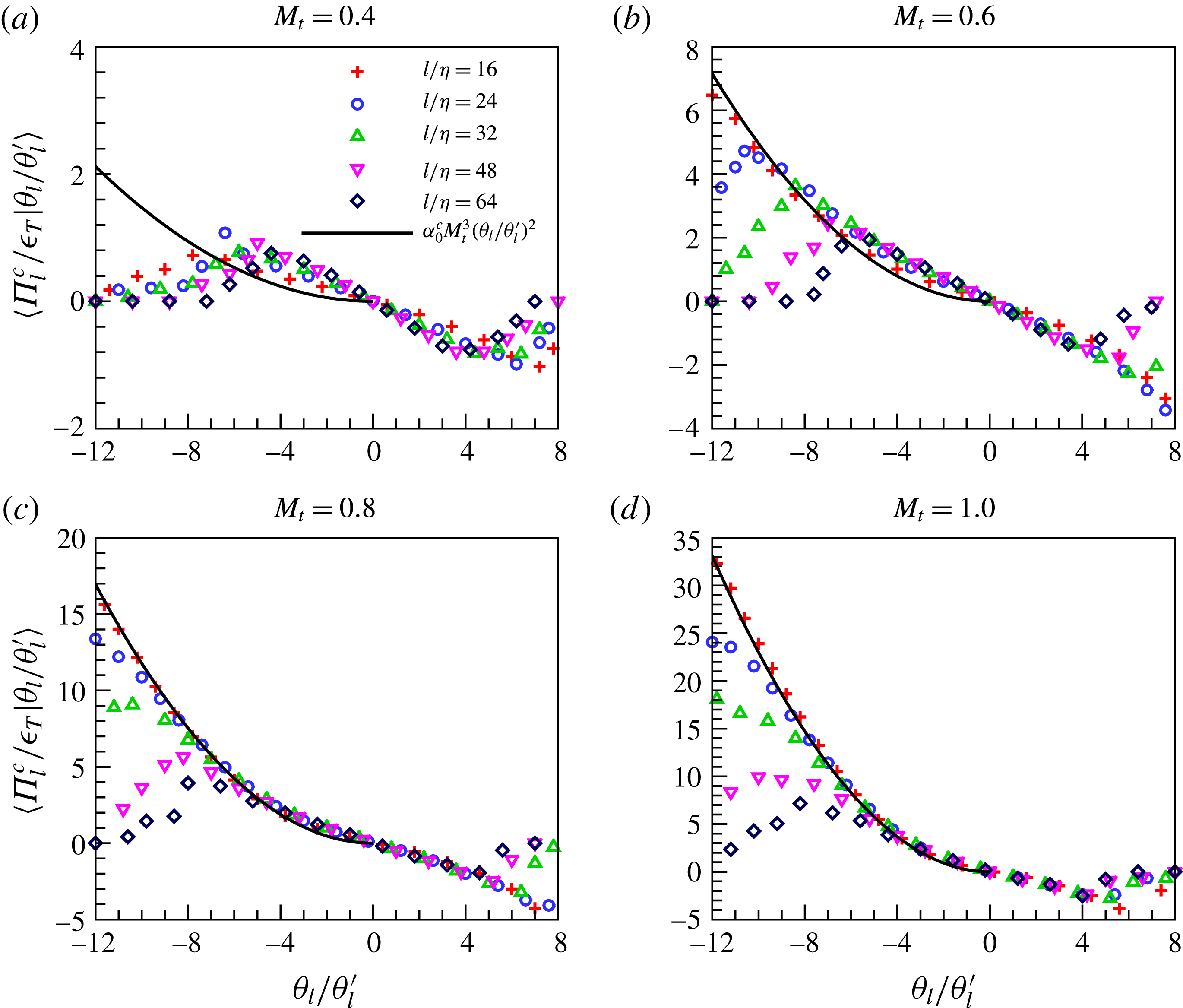
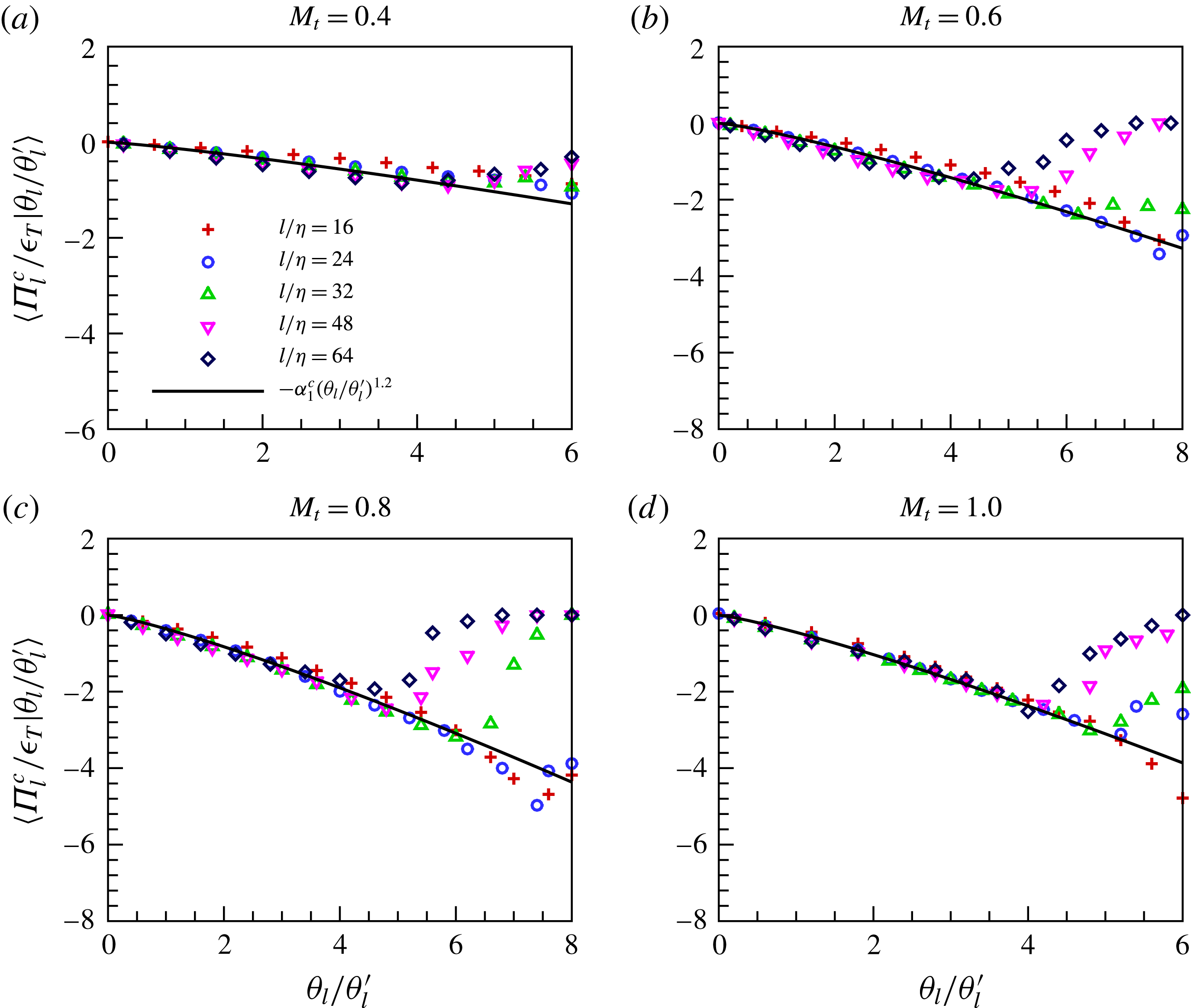
1 Introduction
The inter-scale energy transfer is of much concern in both the theory and large eddy simulation (LES) of turbulence, and has been extensively studied using the filtering technique in incompressible turbulence (Piomelli et al. Reference Piomelli, Cabot, Moin and Lee1991; Domaradzki, Liu & Brachet Reference Domaradzki, Liu and Brachet1993; Kerr, Domaradzki & Barbier Reference Kerr, Domaradzki and Barbier1995; Cimarelli & Meneveau Reference Cerutti and Meneveau1997; Tao, Katz & Meneveau Reference Tao, Katz and Meneveau2002; Eyink Reference Eyink2005; Aluie & Eyink Reference Aluie and Eyink2009; Domaradzki, Teaca & Carati Reference Domaradzki, Teaca and Carati2009; Eyink & Aluie Reference Eyink and Aluie2009). The energy-cascade hypothesis indicates that in the statistical sense, kinetic energy is generated at large scales, transferred to gradually smaller scales and dissipated finally by viscosity at small scales which are close to the Kolmogorov length scale. Actually, the backscatter of energy, i.e. the local reverse transfer of energy from small scales to large scales, can be identified as negative values of the subgrid-scale (SGS) flux in the filtering velocity of turbulence. The presence of local energy backscatter brings great challenges to LES modelling, because overestimation of the energy backscatter can cause simulations to become numerically unstable, while underestimation of the energy backscatter can lead to excessive SGS dissipation. A good understanding of the physics of inter-scale energy transfer is desirable to improve the SGS models in LES of turbulence (Piomelli et al. Reference Piomelli, Cabot, Moin and Lee1991; Domaradzki & Saiki Reference Domaradzki and Saiki1997; Jimenez & Moser Reference Jimenez and Moser2000; Meneveau & Katz Reference Meneveau and Katz2000; Anderson & Domaradzki Reference Anderson and Domaradzki2012; Cimarelli & Angelis Reference Cimarelli and Angelis2014).
Piomelli et al. (Reference Piomelli, Cabot, Moin and Lee1991) conducted a numerical investigation of SGS backscatter to determine the extent and magnitude of the energy transfer from small scales to large scales. They pointed out that accurate modelling of SGS backscatter events is required in LES of turbulence. Domaradzki et al. (Reference Domaradzki, Liu and Brachet1993) and Kerr et al. (Reference Kerr, Domaradzki and Barbier1995) studied the SGS energy transfer in both spectral and physical space representations through direct numerical simulation of incompressible isotropic turbulence. They found that both forward and inverse SGS transfer of energy are significant in the dynamics of resolved scales. Cimarelli & Meneveau (Reference Cerutti and Meneveau1997) studied intermittency of SGS energy flux in incompressible isotropic turbulence. They showed that the spatial distribution of SGS energy flux is highly intermittent, with the highest peaks localized on points or lines, and with sheet-like structures of weaker SGS flux. Moreover, the SGS flux is slightly more intermittent than the longitudinal velocity structure functions. Borue & Orszag (Reference Borue and Orszag1998) analysed the relationship between the SGS energy flux and the locally averaged energy dissipation rate in numerical simulations of forced incompressible isotropic turbulence. They found that predicting the locally averaged energy dissipation rate through inertial-range quantities such as the local SGS energy flux is limited, due to the weak correlation between the local SGS energy flux and the locally averaged energy dissipation rate. Tao et al. (Reference Tao, Katz and Meneveau2002) investigated the statistical geometry of subgrid-scale stresses in a turbulent flow in the core region of a square duct by holographic particle image velocimetry measurements. Their study revealed the relationships of high positive (or high negative) SGS dissipation and SGS stress topology (or strain-rate topology). It is worth noting that locality properties of energy transfer in incompressible turbulence have attracted much attention (Eyink Reference Eyink2005; Domaradzki & Carati Reference Domaradzki and Carati2007a ,Reference Domaradzki and Carati b ; Aluie & Eyink Reference Aluie and Eyink2009; Domaradzki et al. Reference Domaradzki, Teaca and Carati2009; Eyink & Aluie Reference Eyink and Aluie2009).
The inter-scale transfer of kinetic energy in compressible turbulence is more complex and less understood, as compared to the situation of incompressible turbulence. In compressible turbulence, there are complex nonlinear interactions of vortices, acoustic waves, shock waves and expansion-like waves, leading to the strong couplings between the velocity field and thermodynamic fields (Samtaney, Pullin & Kosovic Reference Samtaney, Pullin and Kosovic2001; Pirozzoli & Grasso Reference Pirozzoli and Grasso2004; Petersen & Livescu Reference Petersen and Livescu2010; Suman & Girimaji Reference Suman and Girimaji2011; Jagannathan & Donzis Reference Jagannathan and Donzis2016; Quadros, Sinha & Larsson Reference Quadros, Sinha and Larsson2016; Yang et al. Reference Yang, Wang, Shi, Xiao, He and Chen2016b ; Wang, Gotoh & Watanabe Reference Wang, Gotoh and Watanabe2017a ). Kida & Orszag (Reference Kida and Orszag1992) investigated the statistical properties of decaying compressible isotropic turbulence. They reported that the energy exchange between the kinetic and internal components through the pressure-dilatation interaction can be negligible for the case that the compressive ratios are small. If the compressive ratios are large, a periodic energy exchange between the compressive component of kinetic energy and the internal energy leads to a decaying oscillation of kinetic energy. Miura & Kida (Reference Miura and Kida1995) employed Helmholtz decomposition of density-weighted velocity to study transfer of compressive and rotational kinetic energies in a three-dimensional forced compressible isotropic turbulence. They observed the periodic exchange of the compressive kinetic energy and internal energy. Aluie (Reference Aluie2011, Reference Aluie2013) proved that inter-scale transfer of kinetic energy in compressible turbulence is dominated by local interactions, under the assumption that the pressure-dilatation cospectrum decays at a sufficiently rapid rate. The result was further verified by numerical simulations of both forced and decaying compressible isotropic turbulence (Aluie, Li & Li Reference Aluie, Li and Li2012). Kritsuk, Wagner & Norman (Reference Kritsuk, Wagner and Norman2013) reconstructed an exact fourth-order relation derived analytically from the Navier–Stokes equations by numerical simulation of three-dimensional supersonic isothermal turbulence. Their analysis supported a Kolmogorov-like inertial energy cascade in supersonic turbulence. Wang et al. (Reference Wang, Yang, Shi, Xiao, He and Chen2013) investigated kinetic energy transfer in numerical simulation of compressible isotropic turbulence by applying large-scale forces to both solenoidal and compressive components of the velocity field. They reported that the SGS kinetic energy flux of the compressive mode is significantly larger than that of the solenoidal mode in the inertial range, due to the effect of sheet-like shock waves of large scale generated in the simulated flow.
The interaction between turbulent flow and a normal shock wave is very important in many areas, including hypersonic combustion and astrophysics. Recently, there have been some interesting studies on isotropic turbulence interacting with a normal shock wave (Livescu & Ryu Reference Livescu and Ryu2016; Quadros et al.
Reference Quadros, Sinha and Larsson2016; Livescu & Li Reference Livescu and Li2017). Quadros et al. (Reference Quadros, Sinha and Larsson2016) investigated the turbulent energy flux generated by the interaction between isotropic turbulence and a normal shock wave, by using the linear interaction approximation (LIA) and direct numerical simulation (DNS). They analysed the vortical, entropy and acoustic components of the energy flux correlation behind the shock, and found that the energy flux correlation is a strong function of the shock strength and the angle of incidence of the upstream disturbance wave. It was shown that if the shock wave width is much smaller than the turbulence scales and the upstream turbulent Mach number is small, the shock–turbulence interaction can be described by LIA (Ryu & Livescu Reference Ryu and Livescu2014; Tian et al.
Reference Tian, Jaberi, Li and Livescu2017). Livescu & Li (Reference Livescu and Li2017) generated DNS post-shock data at a Taylor Reynolds number of approximately
 $180$
using LIA, and analysed the SGS flux of kinetic energy in the shock–turbulence interaction problem. They found that for the isotropic turbulence at small turbulent Mach number, the asymmetry of the probability density function (PDF) of SGS flux is decreased, and the SGS backscatter is enhanced, after interacting with the shock wave. Livescu & Ryu (Reference Livescu and Ryu2016) studied the influence of the shock interaction on the divergence of the Lamb vector. They pointed out that the divergence of the Lamb vector plays an important role in the velocity divergence equation and the noise generated by compressible turbulence.
Recently, there have been some interesting studies addressing the effect of combustion on the kinetic energy transfer in compressible turbulent reacting flows (O’Brien et al. Reference O’Brien, Urzay, Ihme, Moin and Saghafian2014; Towery et al. Reference Towery, Poludnenko, Urzay, O’Brien, Ihme and Hamlington2016; O’Brien et al. Reference O’Brien, Towery, Hamlington, Ihme, Poludnenko and Urzay2017), and the effect of the electromagnetic field on the kinetic energy transfer in compressible magnetohydrodynamic (MHD) turbulence and Vlasov–Maxwell turbulence (Yang et al. Reference Yang, Shi, Wan, Matthaeus and Chen2016a , Reference Yang, Matthaeus, Parashar, Haggerty, Roytershteyn, Daughton, Wan, Shi and Chen2017a ,Reference Yang, Matthaeus, Parashar, Wu, Wan, Shi, Chen, Roytershteyn and Daughton b ,Reference Yang, Matthaeus, Shi, Wan and Chen c ). O’Brien et al. (Reference O’Brien, Urzay, Ihme, Moin and Saghafian2014) investigated the dynamics of the backscatter of kinetic energy in reacting and inert supersonic, time evolving hydrogen–air turbulent mixing layers. They reported that backscatter of kinetic energy occurs primarily in regions undergoing volumetric flow expansion. Towery et al. (Reference Towery, Poludnenko, Urzay, O’Brien, Ihme and Hamlington2016) examined the kinetic energy transfer by advective processes in turbulent premixed reacting flows by performing direct numerical simulation of a statistically planar turbulent premixed flame. They concluded that advective processes in premixed reacting flows have significant contributions to the energy backscatter near the scale of the flame. O’Brien et al. (Reference O’Brien, Towery, Hamlington, Ihme, Poludnenko and Urzay2017) studied the kinetic energy transfer between turbulence and flames by direct numerical simulations of a turbulent premixed flame. They found that small amounts of enthalpy created by combustion heat release are transformed into small-scale kinetic energy by means of the SGS pressure-gradient velocity correlation, and the resulting overload of SGS kinetic energy is transferred to the resolved scales through SGS backscatter. Yang et al. (Reference Yang, Shi, Wan, Matthaeus and Chen2016a ) and Yang et al. (Reference Yang, Matthaeus, Shi, Wan and Chen2017c ) investigated energy transfer across scales in three-dimensional compressible MHD turbulence. They showed that energy fluxes due to pressure dilatation and SGS mass flux are greater with more compression. The conversion between kinetic and internal energy by pressure dilatation is dominated by the largest-scale contributions. Yang et al. (Reference Yang, Matthaeus, Parashar, Haggerty, Roytershteyn, Daughton, Wan, Shi and Chen2017a ) and Yang et al. (Reference Yang, Matthaeus, Parashar, Wu, Wan, Shi, Chen, Roytershteyn and Daughton2017b ) studied energy transfer in Vlasov–Maxwell turbulence. They revealed that the pressure–strain interaction can trigger a channel of the energy conversion between fluid flow and random motions, which contains a collision-free generalization of the viscous dissipation in collisional fluid.
In this study, we discuss the inter-scale transfer of kinetic energy in solenoidally forced stationary compressible isotropic turbulence at turbulent Mach numbers ranging from 0.4 to 1.0 and at a Taylor Reynolds number of approximately 250, with a specific focus on the effect of compressibility on the SGS flux of kinetic energy. The rest of the paper is organized as follows. The governing equations and computational method are described in § 2. The one-point statistics of the simulated flow are provided in § 3. The dynamical equations for the filtered kinetic energy and its solenoidal and compressible components are derived in § 4. Numerical results on inter-scale transfer of kinetic energy are presented in § 5. Finally, main conclusions are summarized in § 6.
2 Governing equations and numerical method
A set of reference scales can be introduced to normalize the variables in compressible turbulence. The reference length
 $L_{f}$
, velocity
 $U_{f}$
, density
 $\unicode[STIX]{x1D70C}_{f}$
, pressure
 $p_{f}=\unicode[STIX]{x1D70C}_{f}U_{f}^{2}$
, temperature
 $T_{f}$
, energy per unit volume
 $\unicode[STIX]{x1D70C}_{f}U_{f}^{2}$
, viscosity
 $\unicode[STIX]{x1D707}_{f}$
and thermal conductivity
 $\unicode[STIX]{x1D705}_{f}$
are used respectively (Samtaney et al.
Reference Samtaney, Pullin and Kosovic2001; Wang et al.
Reference Wang, Shi, Wang, Xiao, He and Chen2012a
). There are three reference governing parameters: the reference Reynolds number
 $\mathit{Re}\equiv \unicode[STIX]{x1D70C}_{f}U_{f}L_{f}/\unicode[STIX]{x1D707}_{f}$
, the reference Mach number
 $M=U_{f}/c_{f}$
and the reference Prandtl number
 $Pr\equiv \unicode[STIX]{x1D707}_{f}C_{p}/\unicode[STIX]{x1D705}_{f}$
. The speed of sound is defined as
 $c_{f}\equiv \sqrt{\unicode[STIX]{x1D6FE}RT_{f}}$
, where
 $R$
is the specific gas constant.
 $\unicode[STIX]{x1D6FE}\equiv C_{p}/C_{v}$
is the ratio of specific heat at constant pressure
 $C_{p}$
to that at constant volume
 $C_{v}$
, which is assumed to be equal to
 $1.4$
. The parameter
 $\unicode[STIX]{x1D6FC}$
is defined as
 $\unicode[STIX]{x1D6FC}\equiv Pr\,\mathit{Re}(\unicode[STIX]{x1D6FE}-1)M^{2}$
. The parameter
 $Pr$
is assumed to be equal to
 $0.7$
.
The following dimensionless Navier–Stokes equations in conservation form are solved numerically in our study (Samtaney et al. Reference Samtaney, Pullin and Kosovic2001; Wang et al. Reference Wang, Shi, Wang, Xiao, He and Chen2012a )
 $$\begin{eqnarray}\displaystyle & \displaystyle \frac{\unicode[STIX]{x2202}\unicode[STIX]{x1D70C}}{\unicode[STIX]{x2202}t}+\frac{\unicode[STIX]{x2202}(\unicode[STIX]{x1D70C}u_{j})}{\unicode[STIX]{x2202}x_{j}}=0, & \displaystyle\end{eqnarray}$$
 $$\begin{eqnarray}\displaystyle & \displaystyle \frac{\unicode[STIX]{x2202}(\unicode[STIX]{x1D70C}u_{i})}{\unicode[STIX]{x2202}t}+\frac{\unicode[STIX]{x2202}\left[\unicode[STIX]{x1D70C}u_{i}u_{j}+p\unicode[STIX]{x1D6FF}_{ij}\right]}{\unicode[STIX]{x2202}x_{j}}=\frac{1}{\mathit{Re}}\frac{\unicode[STIX]{x2202}\unicode[STIX]{x1D70E}_{ij}}{\unicode[STIX]{x2202}x_{j}}+{\mathcal{F}}_{i}, & \displaystyle\end{eqnarray}$$
 $$\begin{eqnarray}\displaystyle & \displaystyle \frac{\unicode[STIX]{x2202}{\mathcal{E}}}{\unicode[STIX]{x2202}t}+\frac{\unicode[STIX]{x2202}\left[({\mathcal{E}}+p)u_{j}\right]}{\unicode[STIX]{x2202}x_{j}}=\frac{1}{\unicode[STIX]{x1D6FC}}\frac{\unicode[STIX]{x2202}}{\unicode[STIX]{x2202}x_{j}}\bigg(\unicode[STIX]{x1D705}\frac{\unicode[STIX]{x2202}T}{\unicode[STIX]{x2202}x_{j}}\bigg)+\frac{1}{\mathit{Re}}\frac{\unicode[STIX]{x2202}(\unicode[STIX]{x1D70E}_{ij}u_{i})}{\unicode[STIX]{x2202}x_{j}}-\unicode[STIX]{x1D6EC}+{\mathcal{F}}_{j}u_{j}, & \displaystyle\end{eqnarray}$$
 $$\begin{eqnarray}\displaystyle & \displaystyle p=\unicode[STIX]{x1D70C}T/(\unicode[STIX]{x1D6FE}M^{2}), & \displaystyle\end{eqnarray}$$
where
 $u_{i}$
is the velocity component,
 $\unicode[STIX]{x1D70C}$
is the density,
 $p$
is the pressure and
 $T$
is the temperature. Here,
 ${\mathcal{F}}_{i}$
is a large-scale forcing, and
 $\unicode[STIX]{x1D6EC}$
is a large-scale cooling function. The viscous stress
 $\unicode[STIX]{x1D70E}_{ij}$
is defined as
 $$\begin{eqnarray}\displaystyle & \displaystyle \unicode[STIX]{x1D70E}_{ij}=\unicode[STIX]{x1D707}\bigg(\frac{\unicode[STIX]{x2202}u_{i}}{\unicode[STIX]{x2202}x_{j}}+\frac{\unicode[STIX]{x2202}u_{j}}{\unicode[STIX]{x2202}x_{i}}\bigg)-\frac{2}{3}\unicode[STIX]{x1D707}\unicode[STIX]{x1D703}\unicode[STIX]{x1D6FF}_{ij}, & \displaystyle\end{eqnarray}$$
where,
 $\unicode[STIX]{x1D703}\equiv \unicode[STIX]{x2202}u_{k}/\unicode[STIX]{x2202}x_{k}$
is the velocity divergence. The total energy per unit volume
 ${\mathcal{E}}$
is defined as
 $$\begin{eqnarray}\displaystyle & \displaystyle {\mathcal{E}}=\frac{p}{\unicode[STIX]{x1D6FE}-1}+\frac{1}{2}\unicode[STIX]{x1D70C}(u_{j}u_{j}). & \displaystyle\end{eqnarray}$$
Numerical simulations of compressible isotropic turbulence are performed in a cubic box of
 $2\unicode[STIX]{x03C0}^{3}$
with periodic boundary conditions. A hybrid compact-weighted essentially non-oscillatory (WENO) scheme (Wang et al.
Reference Wang, Wang, Xiao, Shi and Chen2010) is applied for the numerical simulations on a uniform grid with
 $1024^{3}$
grid points. The hybrid scheme combines an eighth-order compact finite difference scheme (Lele Reference Lele1992) in smooth regions and a seventh-order WENO scheme (Balsara & Shu Reference Balsara and Shu2000) in shock regions. The velocity field is forced by fixing the energy spectrum within the two lowest wavenumber shells (Wang et al.
Reference Wang, Wang, Xiao, Shi and Chen2010). The force is only applied to the solenoidal component of the velocity field. A spatially uniform thermal cooling
 $\unicode[STIX]{x1D6EC}$
is applied to sustain the internal energy in a statistically steady state. Sutherland’s law is applied for the non-dimensional temperature-dependent viscosity coefficient
 $\unicode[STIX]{x1D707}$
and thermal conductivity coefficient
 $\unicode[STIX]{x1D705}$
. Grid refinement studies of numerical simulations of compressible isotropic turbulence by the hybrid scheme at a turbulent Mach number of approximately
 $1.0$
were performed in previous works (Wang et al.
Reference Wang, Shi, Wang, Xiao, He and Chen2011, Reference Wang, Shi, Wang, Xiao, He and Chen2012a
).
3 One-point statistics of compressible turbulence
The Taylor microscale Reynolds number
 $\mathit{Re}_{\unicode[STIX]{x1D706}}$
and the turbulent Mach number
 $M_{t}$
are defined as (Wang et al.
Reference Wang, Shi, Wang, Xiao, He and Chen2012a
):
 $$\begin{eqnarray}\displaystyle & \displaystyle \mathit{Re}_{\unicode[STIX]{x1D706}}=\mathit{Re}\frac{u^{\prime }\unicode[STIX]{x1D706}\langle \unicode[STIX]{x1D70C}\rangle }{\sqrt{3}\langle \unicode[STIX]{x1D707}\rangle },\quad M_{t}=M\frac{u^{\prime }}{\langle \sqrt{T}\rangle }, & \displaystyle\end{eqnarray}$$
where
 $\langle \rangle$
stands for ensemble average. The root mean square (r.m.s.) value of velocity magnitude is
 $u^{\prime }\equiv \sqrt{\langle u_{1}^{2}+u_{2}^{2}+u_{3}^{2}\rangle }$
. The Taylor microscale
 $\unicode[STIX]{x1D706}$
is defined as
 $$\begin{eqnarray}\displaystyle & \displaystyle \unicode[STIX]{x1D706}=\sqrt{\frac{{u^{\prime }}^{2}}{\left\langle (\unicode[STIX]{x2202}u_{1}/\unicode[STIX]{x2202}x_{1})^{2}+(\unicode[STIX]{x2202}u_{2}/\unicode[STIX]{x2202}x_{2})^{2}+(\unicode[STIX]{x2202}u_{3}/\unicode[STIX]{x2202}x_{3})^{2}\right\rangle }}. & \displaystyle\end{eqnarray}$$
Table 1 summarizes one-point statistics of four simulated flows in our study. The Taylor microscale Reynolds number is close to
 $250$
. The turbulent Mach number ranges from
 $0.4$
to
 $1.0$
. The Kolmogorov length scale is defined as
 $\unicode[STIX]{x1D702}=[\langle \unicode[STIX]{x1D707}/(\mathit{Re}\unicode[STIX]{x1D70C})\rangle ^{3}/\langle \unicode[STIX]{x1D716}_{V}/\unicode[STIX]{x1D70C}\rangle ]^{1/4}$
, where the local viscous dissipation rate of kinetic energy per unit volume is defined as
 $\unicode[STIX]{x1D716}_{V}\equiv \unicode[STIX]{x1D70E}_{ij}\unicode[STIX]{x1D61A}_{ij}/\mathit{Re}$
. The strain-rate tensor is defined as
 $\unicode[STIX]{x1D61A}_{ij}=(1/2)(\unicode[STIX]{x2202}u_{i}/\unicode[STIX]{x2202}x_{j}+\unicode[STIX]{x2202}u_{j}/\unicode[STIX]{x2202}x_{i})$
. The average viscous dissipation is defined as
 $\unicode[STIX]{x1D716}_{0}=\langle \unicode[STIX]{x1D716}_{V}\rangle$
. The resolution parameter
 $\unicode[STIX]{x1D702}/\unicode[STIX]{x0394}x$
is in the range
 $1.00\leqslant \unicode[STIX]{x1D702}/\unicode[STIX]{x0394}x\leqslant 1.05$
in our simulations, where
 $\unicode[STIX]{x0394}x$
is the grid length in each direction. It is straightforward to show that the resolution parameter
 $k_{max}\unicode[STIX]{x1D702}$
is in the range
 $3.1\leqslant k_{max}\unicode[STIX]{x1D702}\leqslant 3.3$
, where the largest wavenumber
 $k_{max}$
is half of the number of grid points
 $N$
in each direction. Previous grid refinement studies showed that the grid resolutions
 $k_{max}\unicode[STIX]{x1D702}\geqslant 3.1$
are enough for the convergence of flow statistics, including the kinetic energy spectrum at different wavenumbers and the PDFs of velocity divergence and vorticity (Wan et al.
Reference Wan, Oughton, Servidio and Matthaeus2010; Wang et al.
Reference Wang, Shi, Wang, Xiao, He and Chen2011, Reference Wang, Shi, Wang, Xiao, He and Chen2012a
).
Simulation parameters and resulting flow statistics.

The integral length scale
 $L_{f}$
is defined by
 $$\begin{eqnarray}\displaystyle & \displaystyle L_{f}=\frac{3\unicode[STIX]{x03C0}}{2(u^{\prime })^{2}}\int _{0}^{\infty }\frac{E(k)}{k}\,\text{d}k, & \displaystyle\end{eqnarray}$$
where
 $E(k)$
is the spectrum of kinetic energy per unit mass, namely,
 $\int _{0}^{\infty }E(k)\,\text{d}k=(u^{\prime })^{2}/2$
. The ratio
 $L_{f}/\unicode[STIX]{x1D702}$
is in the range
 $226\leqslant L_{f}/\unicode[STIX]{x1D702}\leqslant 237$
in our simulations. The velocity derivative skewness is defined by
 $$\begin{eqnarray}\displaystyle & \displaystyle S_{3}=\frac{\left[\langle (\unicode[STIX]{x2202}u_{1}/\unicode[STIX]{x2202}x_{1})^{3}+(\unicode[STIX]{x2202}u_{2}/\unicode[STIX]{x2202}x_{2})^{3}+(\unicode[STIX]{x2202}u_{3}/\unicode[STIX]{x2202}x_{3})^{3}\rangle \right]/3}{\left\{\langle (\unicode[STIX]{x2202}u_{1}/\unicode[STIX]{x2202}x_{1})^{2}+(\unicode[STIX]{x2202}u_{2}/\unicode[STIX]{x2202}x_{2})^{2}+(\unicode[STIX]{x2202}u_{3}/\unicode[STIX]{x2202}x_{3})^{2}\rangle /3\right\}^{3/2}}. & \displaystyle\end{eqnarray}$$
At
 $M_{t}=0.4$
and
 $0.6$
, the values of
 $S_{3}$
are similar to the typical values of
 $-0.6$
to
 $-0.4$
in incompressible turbulence (Ishihara et al.
Reference Ishihara, Kaneda, Yokokawa, Itakura and Uno2007). At
 $M_{t}=0.8$
and
 $1.0$
, the magnitude of
 $S_{3}$
becomes larger with the increase of
 $M_{t}$
, due to the formation of shocklets in compressible turbulence (Wang et al.
Reference Wang, Shi, Wang, Xiao, He and Chen2011, Reference Wang, Gotoh and Watanabe2017a
; Wang, Gotoh & Watanabe Reference Wang, Gotoh and Watanabe2017b
).
The ensemble average of kinetic energy is governed by the following equation (Wang et al. Reference Wang, Shi, Wang, Xiao, He and Chen2012a ; Jagannathan & Donzis Reference Jagannathan and Donzis2016):
 $$\begin{eqnarray}\displaystyle & \displaystyle \frac{\unicode[STIX]{x2202}}{\unicode[STIX]{x2202}t}\left\langle \frac{1}{2}\unicode[STIX]{x1D70C}u_{i}^{2}\right\rangle =-\unicode[STIX]{x1D716}_{T}+\unicode[STIX]{x1D716}_{inj}, & \displaystyle\end{eqnarray}$$
where, the total dissipation is
 $\unicode[STIX]{x1D716}_{T}=-\langle p\unicode[STIX]{x1D703}\rangle +\unicode[STIX]{x1D716}_{0}$
, i.e. the total conversion rate of kinetic energy into internal energy by the pressure dilatation
 $-\langle p\unicode[STIX]{x1D703}\rangle$
and the viscous dissipation
 $\unicode[STIX]{x1D716}_{0}$
.
 $\unicode[STIX]{x1D716}_{inj}={\mathcal{F}}_{i}u_{i}$
represents the energy injected by the large-scale forcing. We show that the ratio of the average pressure dilatation to the average viscous dissipation is very small:
 $4.3\times 10^{-4}\leqslant -\langle p\unicode[STIX]{x1D703}\rangle /\unicode[STIX]{x1D716}_{0}\leqslant 7.0\times 10^{-2}$
in our simulations, which can be attributed to the cancellation between the positive values of
 $p\unicode[STIX]{x1D703}$
in expansion regions and the negative values of
 $p\unicode[STIX]{x1D703}$
in compression regions (Wang et al.
Reference Wang, Shi, Wang, Xiao, He and Chen2012a
; Jagannathan & Donzis Reference Jagannathan and Donzis2016).
4 Dynamical equations for filtered kinetic energy and its two components
We use a filtering technique (Piomelli et al.
Reference Piomelli, Cabot, Moin and Lee1991; Martin, Piomelli & Candler Reference Martin, Piomelli and Candler2000; Aluie Reference Aluie2011; Wang et al.
Reference Wang, Yang, Shi, Xiao, He and Chen2013) to analyse scale interactions in compressible turbulence. For any field
 $f$
, a filtered field, denoted by an overbar, is defined as
 $$\begin{eqnarray}\displaystyle & \displaystyle \overline{f}(\boldsymbol{x})\equiv \int \,\text{d}^{3}\boldsymbol{r}G_{l}(\boldsymbol{r})f(\boldsymbol{x}+\boldsymbol{r}), & \displaystyle\end{eqnarray}$$
where
 $G_{l}(\boldsymbol{r})\equiv l^{-3}G(\boldsymbol{r}/l)$
is the filter function, and
 $G(\boldsymbol{r})$
is a normalized window function. Here,
 $l$
denotes the filter width associated with the wavelength of the smallest scale retained by the filtering operation. We define the Favre filtered field as
 $\widetilde{f}\equiv \overline{\unicode[STIX]{x1D70C}f}/\overline{\unicode[STIX]{x1D70C}}$
. In our numerical study, a top-hat filter is used, which is calculated in one dimension by (Martin et al.
Reference Martin, Piomelli and Candler2000)
 $$\begin{eqnarray}\displaystyle & \displaystyle \overline{f}_{i}=\frac{1}{4n}\left(f_{i-n}+2\mathop{\sum }_{j=i-n+1}^{i+n-1}f_{j}+f_{i+n}\right), & \displaystyle\end{eqnarray}$$
where, filter width is
 $l=2n\unicode[STIX]{x0394}x$
.
In order to investigate the effect of different filter types on the analysis of kinetic energy transfer, we also consider a Gaussian filter and a sharp spectral filter (Piomelli et al. Reference Piomelli, Cabot, Moin and Lee1991; Pope Reference Pope2000; Sagaut Reference Sagaut2006). In our numerical study, both Gaussian filter and sharp spectral filter are used in Fourier space. The transfer function of the filter in Fourier space is defined as:
 $$\begin{eqnarray}\displaystyle & \displaystyle {\hat{G}}_{l}(\boldsymbol{k})\equiv \int G_{l}(\boldsymbol{r})\text{e}^{-\text{i}\boldsymbol{k}\boldsymbol{\cdot }\boldsymbol{r}}\,\text{d}^{3}\boldsymbol{r}. & \displaystyle\end{eqnarray}$$
The Gaussian filter is given by
 $$\begin{eqnarray}\displaystyle & \displaystyle {\hat{G}}_{l}^{GF}(\boldsymbol{k})=\exp \left(\frac{-k^{2}l^{2}}{24}\right), & \displaystyle\end{eqnarray}$$
where,
 $k=|\boldsymbol{k}|$
. The sharp spectral filter is given by
 $$\begin{eqnarray}\displaystyle & \displaystyle {\hat{G}}_{l}^{SF}(\boldsymbol{k})=H\left(k_{c}-k\right), & \displaystyle\end{eqnarray}$$
where,
 $k_{c}=\unicode[STIX]{x03C0}/l$
. Here, the Heaviside step function
 $H(x)$
is defined as:
 $H(x)=1$
if
 $x\geqslant 0$
; otherwise
 $H(x)=0$
. The filtered field associated with the Gaussian filter is denoted with the superscript ‘GF’. The filtered field associated with the sharp spectral filter is denoted with the superscript ‘SF’.
The filtered equations for the density and momentum are
 $$\begin{eqnarray}\displaystyle & \displaystyle \frac{\unicode[STIX]{x2202}\overline{\unicode[STIX]{x1D70C}}}{\unicode[STIX]{x2202}t}+\frac{\unicode[STIX]{x2202}\left(\overline{\unicode[STIX]{x1D70C}}\widetilde{u}_{j}\right)}{\unicode[STIX]{x2202}x_{j}}=0, & \displaystyle\end{eqnarray}$$
 $$\begin{eqnarray}\displaystyle & \displaystyle \frac{\unicode[STIX]{x2202}\left(\overline{\unicode[STIX]{x1D70C}}\widetilde{u}_{i}\right)}{\unicode[STIX]{x2202}t}+\frac{\unicode[STIX]{x2202}\left[\overline{\unicode[STIX]{x1D70C}}\widetilde{u}_{i}\widetilde{u}_{j}+\overline{p}\unicode[STIX]{x1D6FF}_{ij}\right]}{\unicode[STIX]{x2202}x_{j}}=-\frac{\unicode[STIX]{x2202}\left(\overline{\unicode[STIX]{x1D70C}}\widetilde{\unicode[STIX]{x1D70F}}_{ij}\right)}{\unicode[STIX]{x2202}x_{j}}+\frac{1}{\mathit{Re}}\frac{\unicode[STIX]{x2202}\overline{\unicode[STIX]{x1D70E}}_{ij}}{\unicode[STIX]{x2202}x_{j}}, & \displaystyle\end{eqnarray}$$
where, the subgrid-scale (SGS) stress is
 $\overline{\unicode[STIX]{x1D70C}}\widetilde{\unicode[STIX]{x1D70F}}_{ij}=\overline{\unicode[STIX]{x1D70C}}\left(\widetilde{u_{i}u_{j}}-\widetilde{u}_{i}\widetilde{u}_{j}\right)$
. The appearance of the SGS stress is attributed to the effect of eliminated scales
 ${<}l$
. Here, we do not consider the effect of large-scale external forcing. It is straightforward to derive the filtered equation for the large-scale kinetic energy
 $(1/2)\overline{\unicode[STIX]{x1D70C}}\widetilde{u}_{i}^{2}$
(Aluie Reference Aluie2011, Reference Aluie2013; Wang et al.
Reference Wang, Yang, Shi, Xiao, He and Chen2013)
 $$\begin{eqnarray}\displaystyle & \displaystyle \frac{\unicode[STIX]{x2202}}{\unicode[STIX]{x2202}t}\left(\frac{1}{2}\overline{\unicode[STIX]{x1D70C}}\widetilde{u}_{i}^{2}\right)+J_{l}=-\unicode[STIX]{x1D6F7}_{l}-\unicode[STIX]{x1D6F1}_{l}-D_{l}. & \displaystyle\end{eqnarray}$$
Here,
 $J_{l}$
is the space transport of large-scale kinetic energy.
 $\unicode[STIX]{x1D6F7}_{l}$
is the large-scale pressure-dilatation term.
 $\unicode[STIX]{x1D6F1}_{l}$
is the SGS kinetic energy flux.
 $D_{l}$
is the viscous dissipation term. These terms are defined as
 $$\begin{eqnarray}\displaystyle & \displaystyle J_{l}\equiv \frac{\unicode[STIX]{x2202}}{\unicode[STIX]{x2202}x_{j}}\left(\frac{1}{2}\overline{\unicode[STIX]{x1D70C}}\widetilde{u}_{i}^{2}\widetilde{u}_{j}+\overline{p}\widetilde{u}_{j}+\overline{\unicode[STIX]{x1D70C}}\widetilde{\unicode[STIX]{x1D70F}}_{ij}\widetilde{u}_{i}-\frac{\widetilde{u}_{i}\overline{\unicode[STIX]{x1D70E}}_{ij}}{Re}\right), & \displaystyle\end{eqnarray}$$
 $$\begin{eqnarray}\displaystyle & \displaystyle \unicode[STIX]{x1D6F7}_{l}\equiv -\overline{p}\frac{\unicode[STIX]{x2202}\widetilde{u}_{i}}{\unicode[STIX]{x2202}x_{i}}, & \displaystyle\end{eqnarray}$$
 $$\begin{eqnarray}\displaystyle & \displaystyle \unicode[STIX]{x1D6F1}_{l}\equiv -\overline{\unicode[STIX]{x1D70C}}\widetilde{\unicode[STIX]{x1D70F}}_{ij}\frac{\unicode[STIX]{x2202}\widetilde{u}_{i}}{\unicode[STIX]{x2202}x_{j}}=-\overline{\unicode[STIX]{x1D70C}}\widetilde{\unicode[STIX]{x1D70F}}_{ij}\widetilde{\unicode[STIX]{x1D61A}}_{ij}, & \displaystyle\end{eqnarray}$$
and,
 $$\begin{eqnarray}\displaystyle & \displaystyle D_{l}\equiv \frac{\overline{\unicode[STIX]{x1D70E}}_{ij}}{Re}\frac{\unicode[STIX]{x2202}\widetilde{u}_{i}}{\unicode[STIX]{x2202}x_{j}}, & \displaystyle\end{eqnarray}$$
where, the large-scale strain tensor
 $\widetilde{\unicode[STIX]{x1D64E}}$
is defined as:
 $\widetilde{\unicode[STIX]{x1D61A}}_{ij}\equiv (1/2)\left(\unicode[STIX]{x2202}\widetilde{u}_{i}/\unicode[STIX]{x2202}x_{j}+\unicode[STIX]{x2202}\widetilde{u}_{j}/\unicode[STIX]{x2202}x_{i}\right)$
. The equation for the ensemble average of the filtered kinetic energy can be written as follows:
 $$\begin{eqnarray}\displaystyle & \displaystyle \frac{\unicode[STIX]{x2202}}{\unicode[STIX]{x2202}t}\left\langle \frac{1}{2}\overline{\unicode[STIX]{x1D70C}}\widetilde{u}_{i}^{2}\right\rangle =-\left\langle \unicode[STIX]{x1D6F7}_{l}\right\rangle -\left\langle \unicode[STIX]{x1D6F1}_{l}\right\rangle -\left\langle D_{l}\right\rangle . & \displaystyle\end{eqnarray}$$
Now we define a filtered density-weighted variable
 $\widetilde{\boldsymbol{w}}$
as
 $\widetilde{\boldsymbol{w}}=\sqrt{\overline{\unicode[STIX]{x1D70C}}}\widetilde{\boldsymbol{u}}$
. It is easy to see that
 $\widetilde{\boldsymbol{w}}^{2}/2$
represents the kinetic energy of the filtered fields
 $\overline{\unicode[STIX]{x1D70C}}$
and
 $\widetilde{\boldsymbol{u}}$
. The filtered equation for
 $\widetilde{\boldsymbol{w}}$
reads
 $$\begin{eqnarray}\displaystyle & \displaystyle \frac{\unicode[STIX]{x2202}\widetilde{w}_{i}}{\unicode[STIX]{x2202}t}+\widetilde{u}_{j}\frac{\unicode[STIX]{x2202}\widetilde{w}_{i}}{\unicode[STIX]{x2202}x_{j}}+\frac{\widetilde{w}_{i}}{2}\frac{\unicode[STIX]{x2202}\widetilde{u}_{j}}{\unicode[STIX]{x2202}x_{j}}=-\frac{1}{\sqrt{\overline{\unicode[STIX]{x1D70C}}}}\frac{\unicode[STIX]{x2202}\overline{p}}{\unicode[STIX]{x2202}x_{i}}-\frac{1}{\sqrt{\overline{\unicode[STIX]{x1D70C}}}}\frac{\unicode[STIX]{x2202}\overline{\unicode[STIX]{x1D70C}}\widetilde{\unicode[STIX]{x1D70F}}_{ij}}{\unicode[STIX]{x2202}x_{j}}+\frac{1}{\sqrt{\overline{\unicode[STIX]{x1D70C}}}Re}\frac{\unicode[STIX]{x2202}\overline{\unicode[STIX]{x1D70E}}_{ij}}{\unicode[STIX]{x2202}x_{j}}. & \displaystyle\end{eqnarray}$$
Helmholtz decomposition of the
 $\widetilde{\boldsymbol{w}}$
yields:
 $\widetilde{\boldsymbol{w}}=\widetilde{\boldsymbol{w}}^{s}+\widetilde{\boldsymbol{w}}^{c}$
, where
 $\widetilde{\boldsymbol{w}}^{s}$
is the solenoidal component and
 $\widetilde{\boldsymbol{w}}^{c}$
is the compressible component. The two components
 $\widetilde{\boldsymbol{w}}^{s}$
and
 $\widetilde{\boldsymbol{w}}^{c}$
satisfy the following relations:
 $\unicode[STIX]{x1D735}\boldsymbol{\cdot }\widetilde{\boldsymbol{w}}^{s}=0$
and
 $\unicode[STIX]{x1D735}\times \widetilde{\boldsymbol{w}}^{c}=0$
. Multiplying (4.14) by
 $\widetilde{w}_{i}^{X}$
yields:
 $$\begin{eqnarray}\displaystyle & \displaystyle \widetilde{w}_{i}^{X}\frac{\unicode[STIX]{x2202}\widetilde{w}_{i}}{\unicode[STIX]{x2202}t}+\widetilde{w}_{i}^{X}\left(\widetilde{u}_{j}\frac{\unicode[STIX]{x2202}\widetilde{w}_{i}}{\unicode[STIX]{x2202}x_{j}}+\frac{\widetilde{w}_{i}}{2}\frac{\unicode[STIX]{x2202}\widetilde{u}_{j}}{\unicode[STIX]{x2202}x_{j}}\right)=-\frac{\widetilde{w}_{i}^{X}}{\sqrt{\overline{\unicode[STIX]{x1D70C}}}}\frac{\unicode[STIX]{x2202}\overline{p}}{\unicode[STIX]{x2202}x_{i}}-\frac{\widetilde{w}_{i}^{X}}{\sqrt{\overline{\unicode[STIX]{x1D70C}}}}\frac{\unicode[STIX]{x2202}\overline{\unicode[STIX]{x1D70C}}\widetilde{\unicode[STIX]{x1D70F}}_{ij}}{\unicode[STIX]{x2202}x_{j}}+\frac{\widetilde{w}_{i}^{X}}{\sqrt{\overline{\unicode[STIX]{x1D70C}}}Re}\frac{\unicode[STIX]{x2202}\overline{\unicode[STIX]{x1D70E}}_{ij}}{\unicode[STIX]{x2202}x_{j}}, & \displaystyle\end{eqnarray}$$
where,
 $X=s,c$
. Taking an ensemble average of (4.15) gives the filtered equation for the ensemble average of the solenoidal (or compressible) component of the large-scale kinetic energy:
 $$\begin{eqnarray}\displaystyle & \displaystyle \frac{\unicode[STIX]{x2202}}{\unicode[STIX]{x2202}t}\left\langle \frac{1}{2}\left(\widetilde{w}_{i}^{X}\right)^{2}\right\rangle =\left\langle A_{l}^{X}\right\rangle -\left\langle \unicode[STIX]{x1D6F7}_{l}^{X}\right\rangle -\left\langle \unicode[STIX]{x1D6F1}_{l}^{X}\right\rangle -\left\langle D_{l}^{X}\right\rangle . & \displaystyle\end{eqnarray}$$
Here,
 $A_{l}^{X}$
is the nonlinear advection term.
 $\unicode[STIX]{x1D6F7}_{l}^{X}$
is the large-scale pressure-dilatation term.
 $\unicode[STIX]{x1D6F1}_{l}^{X}$
is the SGS kinetic energy flux.
 $D_{l}^{X}$
is the viscous dissipation term. These terms are defined as:
 $$\begin{eqnarray}\displaystyle & \displaystyle A_{l}^{X}\equiv -\widetilde{w}_{i}^{X}\left(\widetilde{u}_{j}\frac{\unicode[STIX]{x2202}\widetilde{w}_{i}}{\unicode[STIX]{x2202}x_{j}}+\frac{\widetilde{w}_{i}}{2}\frac{\unicode[STIX]{x2202}\widetilde{u}_{j}}{\unicode[STIX]{x2202}x_{j}}\right), & \displaystyle\end{eqnarray}$$
 $$\begin{eqnarray}\displaystyle & \displaystyle \unicode[STIX]{x1D6F7}_{l}^{X}\equiv -\overline{p}\frac{\unicode[STIX]{x2202}}{\unicode[STIX]{x2202}x_{i}}\left(\frac{\widetilde{w}_{i}^{X}}{\sqrt{\overline{\unicode[STIX]{x1D70C}}}}\right), & \displaystyle\end{eqnarray}$$
 $$\begin{eqnarray}\displaystyle & \displaystyle \unicode[STIX]{x1D6F1}_{l}^{X}\equiv -\overline{\unicode[STIX]{x1D70C}}\widetilde{\unicode[STIX]{x1D70F}}_{ij}\frac{\unicode[STIX]{x2202}}{\unicode[STIX]{x2202}x_{j}}\left(\frac{\widetilde{w}_{i}^{X}}{\sqrt{\overline{\unicode[STIX]{x1D70C}}}}\right), & \displaystyle\end{eqnarray}$$
and,
 $$\begin{eqnarray}\displaystyle & \displaystyle D_{l}^{X}\equiv \frac{\overline{\unicode[STIX]{x1D70E}}_{ij}}{Re}\frac{\unicode[STIX]{x2202}}{\unicode[STIX]{x2202}x_{j}}\left(\frac{\widetilde{w}_{i}^{X}}{\sqrt{\overline{\unicode[STIX]{x1D70C}}}}\right). & \displaystyle\end{eqnarray}$$
It is straightforward to derive the following relations:
 $\langle A_{l}^{s}+A_{l}^{c}\rangle =0$
,
 $\unicode[STIX]{x1D6F7}_{l}^{s}+\unicode[STIX]{x1D6F7}_{l}^{c}=\unicode[STIX]{x1D6F7}_{l}$
,
 $\unicode[STIX]{x1D6F1}_{l}^{s}+\unicode[STIX]{x1D6F1}_{l}^{c}=\unicode[STIX]{x1D6F1}_{l}$
and
 $D_{l}^{s}+D_{l}^{c}=D_{l}$
.
5 Numerical results on inter-scale transfer of kinetic energy
In this section, we study the statistics of kinetic energy transfer with numerical simulations. We focus on the effect of expansion and compression on the SGS flux of kinetic energy. Moreover, we investigate the Helmholtz decomposition on the SGS flux of kinetic energy.
5.1 Statistics of kinetic energy transfer
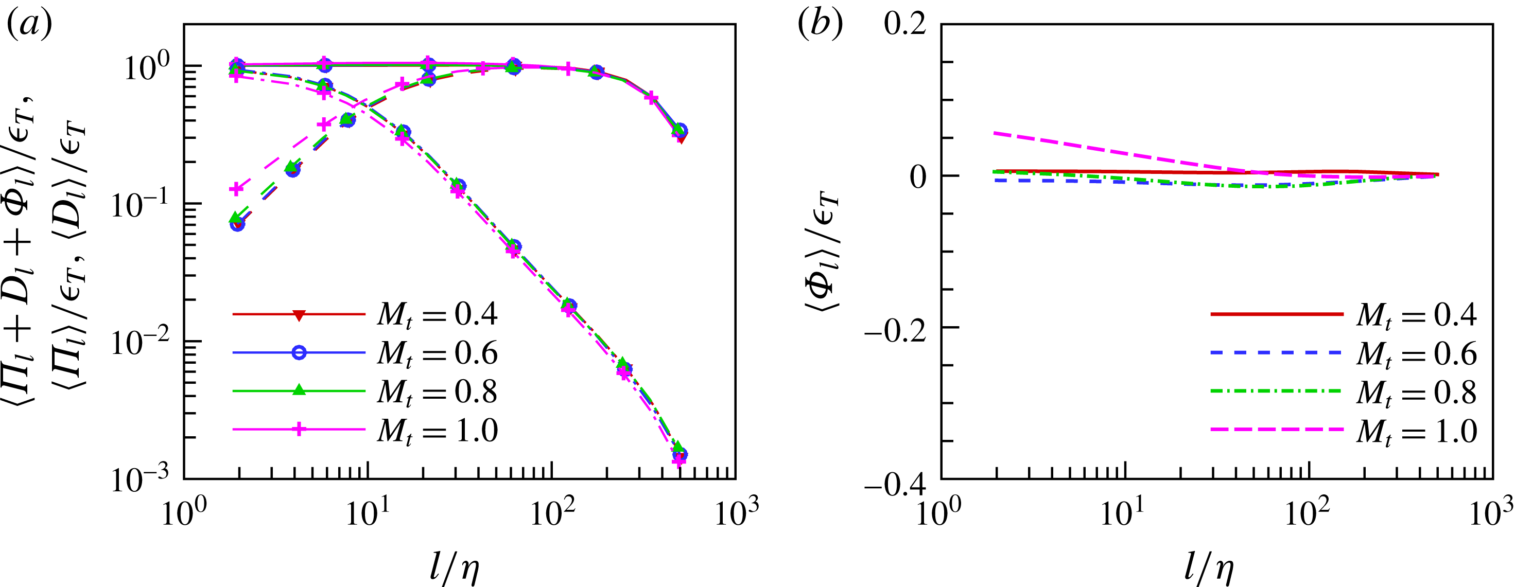
In figure 1(a), we plot ensemble average of energy transfer terms of (4.13) at turbulent Mach numbers
 $M_{t}=0.4,0.6,0.8,1.0$
. The energy transfer terms are normalized by the total dissipation
 $\unicode[STIX]{x1D716}_{T}=-\langle p\unicode[STIX]{x1D703}\rangle +\unicode[STIX]{x1D716}_{0}$
. We find that the overall energy transfer
 $\langle \unicode[STIX]{x1D6F1}_{l}+D_{l}+\unicode[STIX]{x1D6F7}_{l}\rangle /\unicode[STIX]{x1D716}_{T}\approx 1.0$
at scales
 $l/\unicode[STIX]{x1D702}\leqslant 200$
, and
 $\langle \unicode[STIX]{x1D6F1}_{l}+D_{l}+\unicode[STIX]{x1D6F7}_{l}\rangle /\unicode[STIX]{x1D716}_{T}<1.0$
at scales
 $l/\unicode[STIX]{x1D702}>200$
. Thus, the effect of large-scale external forcing is negligible at scales
 $l/\unicode[STIX]{x1D702}\leqslant 200$
. This observation is consistent with a previous theoretical study of kinetic energy transfer in compressible turbulence by Aluie (Reference Aluie2013), where he proved analytically that in the situation of the scale decomposition by the Favre filtering, the kinetic energy injection can be localized to the large scales by a proper stirring, such as a large-scale external acceleration field used in our simulations. It is also worth noting that for the situations of other scale decompositions, the effect of large-scale external forcing on the kinetic energy transfer could be important at all scales. For example, the non-local effect of large-scale forcing was identified in a supersonic isothermal turbulence at the turbulent root-mean-square Mach number 6, which was related with a correlation function of the density field (Falkovich, Fouxon & Oz Reference Falkovich, Fouxon and Oz2010; Wagner et al.
Reference Wagner, Falkovich, Kritsuk and Norman2012). The viscous dissipation
 $\langle D_{l}\rangle /\unicode[STIX]{x1D716}_{T}$
is important at small scales
 $l/\unicode[STIX]{x1D702}\leqslant 10$
, and decays rapidly as the filter width
 $l/\unicode[STIX]{x1D702}$
increases from
 $10$
. This observation is consistent with previous theoretical analysis of the viscous dissipation in compressible flows (Aluie Reference Aluie2011, Reference Aluie2013). The SGS flux
 $\langle \unicode[STIX]{x1D6F1}_{l}\rangle /\unicode[STIX]{x1D716}_{T}$
is close to
 $1.0$
at scales
 $30\leqslant l/\unicode[STIX]{x1D702}\leqslant 200$
. All these terms are insensitive to the change of turbulent Mach number in our simulations. In figure 1(b), we plot ensemble average of pressure-dilatation term
 $\langle \unicode[STIX]{x1D6F7}_{l}\rangle /\unicode[STIX]{x1D716}_{T}$
. We show that
 $\langle \unicode[STIX]{x1D6F7}_{l}\rangle /\unicode[STIX]{x1D716}_{T}$
is smaller than
 $0.05$
at scales
 $l/\unicode[STIX]{x1D702}\geqslant 10$
for all four turbulent Mach numbers, indicating that the net contribution of pressure dilatation to the kinetic energy transfer is negligibly small at scales
 $l/\unicode[STIX]{x1D702}\geqslant 10$
.
Ensemble average of energy transfer terms at turbulent Mach numbers
 $M_{t}=0.4,0.6,0.8,1.0$
. (a) Solid lines:
 $\langle \unicode[STIX]{x1D6F1}_{l}+D_{l}+\unicode[STIX]{x1D6F7}_{l}\rangle /\unicode[STIX]{x1D716}_{T}$
; dashed lines:
 $\langle \unicode[STIX]{x1D6F1}_{l}\rangle /\unicode[STIX]{x1D716}_{T}$
; dash-dotted lines:
 $\langle D_{l}\rangle /\unicode[STIX]{x1D716}_{T}$
. (b)
 $\langle \unicode[STIX]{x1D6F7}_{l}\rangle /\unicode[STIX]{x1D716}_{T}$
.

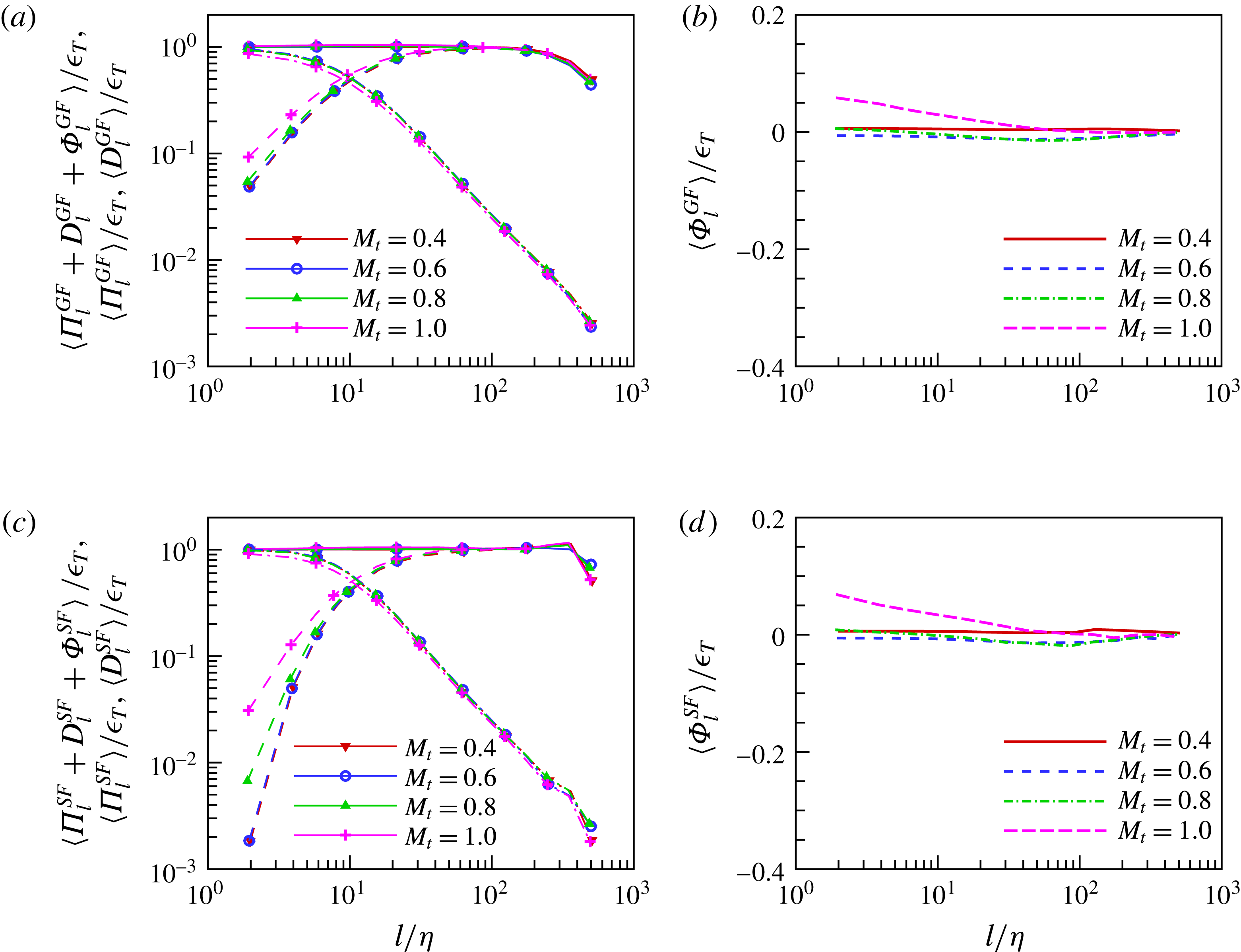
In figure 2, we plot the ensemble averages of the energy transfer terms of (4.13) by using the Gaussian filter and the sharp spectral filter. We find that the results by using three different filters are quite similar at
 $l/\unicode[STIX]{x1D702}\geqslant 10$
. Particularly, the top-hat filter and the Gaussian filter give nearly identical results at all scales of the filter length
 $l$
. The results by using the sharp spectral filter are slightly different: the SGS flux
 $\langle \unicode[STIX]{x1D6F1}_{l}^{SF}\rangle /\unicode[STIX]{x1D716}_{T}$
is remarkably small at scales
 $l/\unicode[STIX]{x1D702}\leqslant 10$
, especially, for small turbulent Mach numbers
 $M_{t}=0.4,0.6$
; As turbulent Mach number increases,
 $\langle \unicode[STIX]{x1D6F1}_{l}^{SF}\rangle /\unicode[STIX]{x1D716}_{T}$
increases rapidly at scales
 $l/\unicode[STIX]{x1D702}\leqslant 10$
, for
 $0.8\leqslant M_{t}\leqslant 1.0$
. It is worth noting that the net contribution of pressure dilatation to the kinetic energy transfer is always negligibly small at scales
 $l/\unicode[STIX]{x1D702}\geqslant 10$
for different types of filters.
Ensemble average of energy transfer terms using the Gaussian filter and the sharp spectral filter. (a) Solid lines:
 $\langle \unicode[STIX]{x1D6F1}_{l}^{GF}+D_{l}^{GF}+\unicode[STIX]{x1D6F7}_{l}^{GF}\rangle /\unicode[STIX]{x1D716}_{T}$
; dashed lines:
 $\langle \unicode[STIX]{x1D6F1}_{l}^{GF}\rangle /\unicode[STIX]{x1D716}_{T}$
; dash-dotted lines:
 $\langle D_{l}^{GF}\rangle /\unicode[STIX]{x1D716}_{T}$
; (b)
 $\langle \unicode[STIX]{x1D6F7}_{l}^{GF}\rangle /\unicode[STIX]{x1D716}_{T}$
; (c) solid lines:
 $\langle \unicode[STIX]{x1D6F1}_{l}^{SF}+D_{l}^{SF}+\unicode[STIX]{x1D6F7}_{l}^{SF}\rangle /\unicode[STIX]{x1D716}_{T}$
; dashed lines:
 $\langle \unicode[STIX]{x1D6F1}_{l}^{SF}\rangle /\unicode[STIX]{x1D716}_{T}$
; dash-dotted lines:
 $\langle D_{l}^{SF}\rangle /\unicode[STIX]{x1D716}_{T}$
; (d)
 $\langle \unicode[STIX]{x1D6F7}_{l}^{SF}\rangle /\unicode[STIX]{x1D716}_{T}$
.

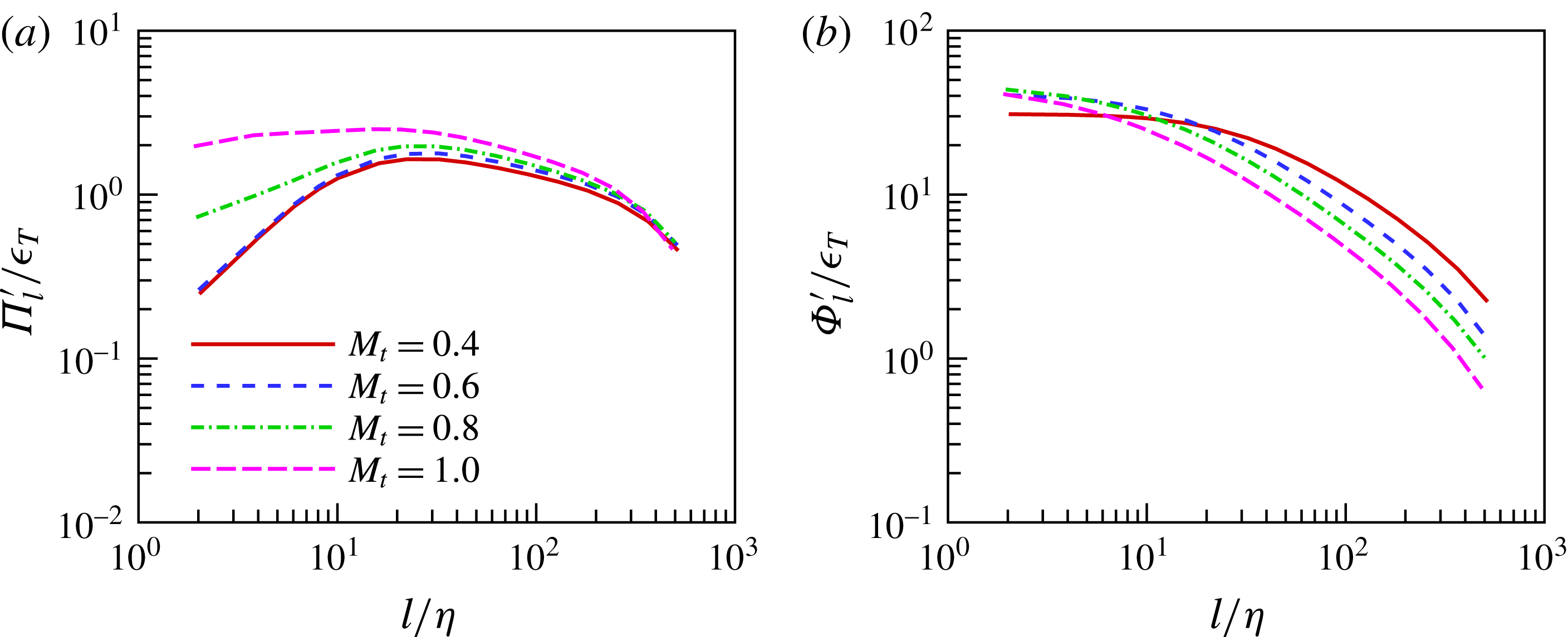
The root mean square (r.m.s.) values of SGS flux and pressure dilatation are defined as
 $\unicode[STIX]{x1D6F1}_{l}^{\prime }=\sqrt{\langle (\unicode[STIX]{x1D6F1}_{l}-\langle \unicode[STIX]{x1D6F1}_{l}\rangle )^{2}\rangle }$
and
 $\unicode[STIX]{x1D6F7}_{l}^{\prime }=\sqrt{\langle (\unicode[STIX]{x1D6F7}_{l}-\langle \unicode[STIX]{x1D6F7}_{l}\rangle )^{2}\rangle }$
. We plot
 $\unicode[STIX]{x1D6F1}_{l}^{\prime }/\unicode[STIX]{x1D716}_{T}$
and
 $\unicode[STIX]{x1D6F7}_{l}^{\prime }/\unicode[STIX]{x1D716}_{T}$
in figures 3(a) and 3(b) respectively. We observe that r.m.s. value of SGS flux
 $\unicode[STIX]{x1D6F1}_{l}^{\prime }/\unicode[STIX]{x1D716}_{T}$
becomes larger with an increase of turbulent Mach number for
 $M_{t}=0.8,1.0$
, particularly, at relatively small scales
 $l/\unicode[STIX]{x1D702}\leqslant 30$
. Thus, as the turbulent Mach number increases, the compressibility effect will enhance the local transfer of kinetic energy by the SGS stress. It is interesting to observe that
 $\unicode[STIX]{x1D6F7}_{l}^{\prime }/\unicode[STIX]{x1D716}_{T}>1.0$
at scales
 $l/\unicode[STIX]{x1D702}\leqslant 200$
for all four turbulent Mach numbers.
 $\unicode[STIX]{x1D6F7}_{l}^{\prime }/\unicode[STIX]{x1D716}_{T}$
becomes larger as the filter width
 $l/\unicode[STIX]{x1D702}$
decreases. Particularly,
 $\unicode[STIX]{x1D6F7}_{l}^{\prime }/\unicode[STIX]{x1D716}_{T}>20$
at small scales
 $l/\unicode[STIX]{x1D702}\leqslant 10$
. Thus, the pressure dilatation plays an important role in the local conversion between kinetic energy and internal energy. It is worth noting that
 $\langle \unicode[STIX]{x1D6F7}_{l}\rangle /\unicode[STIX]{x1D716}_{T}\ll \unicode[STIX]{x1D6F7}_{l}^{\prime }/\unicode[STIX]{x1D716}_{T}$
. The contribution of pressure dilatation nearly vanishes after ensemble average, due to the cancellation between compression and expansion works. The observations are consistent with previous studies on compressible turbulence (Aluie et al.
Reference Aluie, Li and Li2012; Wang et al.
Reference Wang, Shi, Wang, Xiao, He and Chen2012a
; Jagannathan & Donzis Reference Jagannathan and Donzis2016).
The r.m.s. values of SGS flux and pressure dilatation at turbulent Mach numbers
 $M_{t}=0.4,0.6,0.8,1.0$
. (a)
 $\unicode[STIX]{x1D6F1}_{l}^{\prime }/\unicode[STIX]{x1D716}_{T}$
; (b)
 $\unicode[STIX]{x1D6F7}_{l}^{\prime }/\unicode[STIX]{x1D716}_{T}$
.

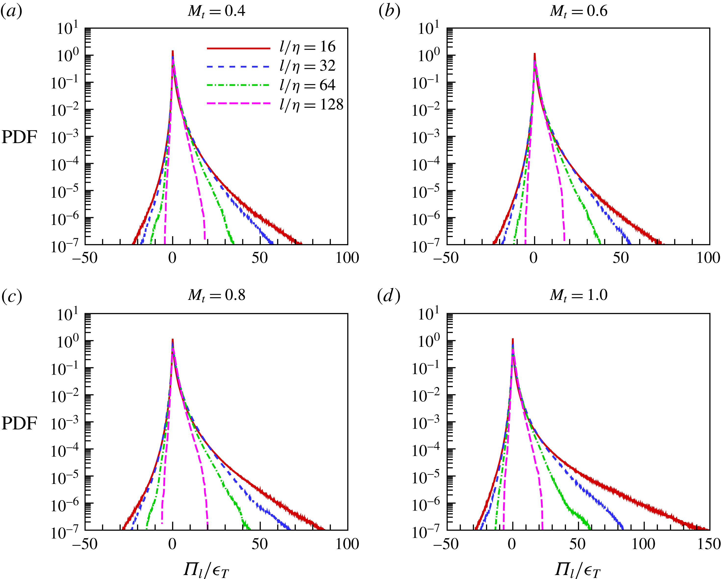
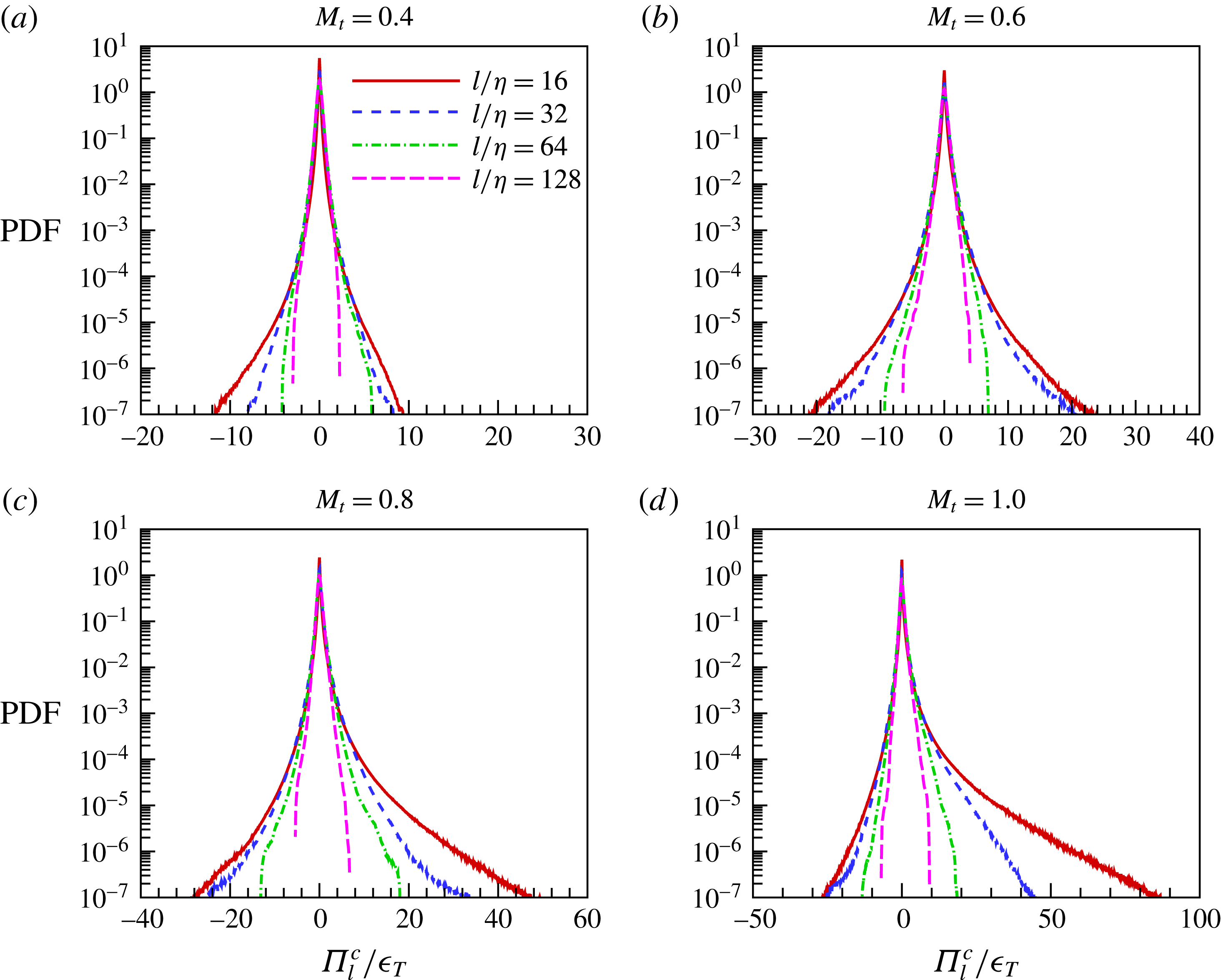
We depict the probability density function (PDF) of the normalized SGS flux
 $\unicode[STIX]{x1D6F1}_{l}/\unicode[STIX]{x1D716}_{T}$
at turbulent Mach numbers
 $M_{t}=0.4,0.6,0.8,1.0$
in figure 4. We observe that the negative value of SGS flux occurs in some flow regions as indicated by the negative side of the PDF. The negative value of SGS flux can be interpreted as the SGS backscatter of kinetic energy, i.e. the reverse flux of kinetic energy from small scales to large scales. The PDF of SGS flux exhibits a skewness toward the positive side, indicating that the kinetic energy transfer due to the SGS stress has a tendency to be from large scales to small scales. The two tails of PDF become longer as the filter width
 $l/\unicode[STIX]{x1D702}$
decreases, due to the fact that local energy transfer is more intermittent at small scales than at large scales. These observations are similar to the situation of incompressible turbulence. As the turbulent Mach number increases, the right tail of PDF of SGS flux becomes longer at
 $M_{t}=0.8,1.0$
, particularly at relatively small scales
 $l/\unicode[STIX]{x1D702}=16,32$
. Thus, the compressibility enhances the local SGS energy transfer from large scales to small scales at
 $M_{t}=0.8,1.0$
.
PDF of the normalized SGS flux
 $\unicode[STIX]{x1D6F1}_{l}/\unicode[STIX]{x1D716}_{T}$
at turbulent Mach numbers
 $M_{t}=0.4,0.6,0.8,1.0$
.

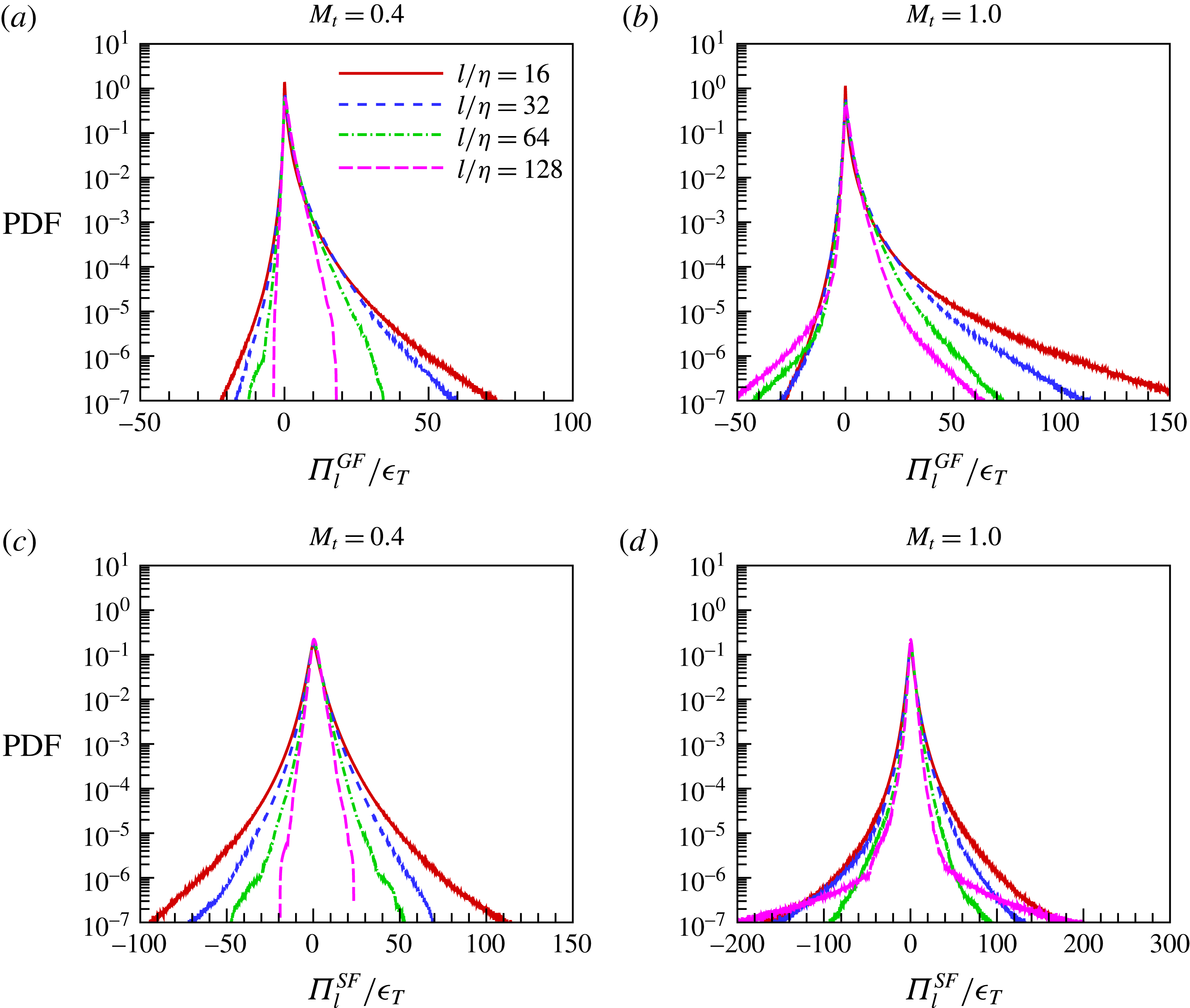
In figure 5, we plot the PDF of the normalized SGS flux by using the Gaussian filter and the sharp spectral filter. We show that the PDF of
 $\unicode[STIX]{x1D6F1}_{l}^{GF}/\unicode[STIX]{x1D716}_{T}$
is similar to that of
 $\unicode[STIX]{x1D6F1}_{l}/\unicode[STIX]{x1D716}_{T}$
, particularly, at
 $M_{t}=0.4$
. The major difference between PDFs of
 $\unicode[STIX]{x1D6F1}_{l}^{GF}/\unicode[STIX]{x1D716}_{T}$
and
 $\unicode[STIX]{x1D6F1}_{l}/\unicode[STIX]{x1D716}_{T}$
is that the PDF tails of
 $\unicode[STIX]{x1D6F1}_{l}^{GF}/\unicode[STIX]{x1D716}_{T}$
are longer than those of
 $\unicode[STIX]{x1D6F1}_{l}/\unicode[STIX]{x1D716}_{T}$
at turbulent Mach number
 $M_{t}=1.0$
and large scales
 $l/\unicode[STIX]{x1D702}=64,128$
. The PDF of
 $\unicode[STIX]{x1D6F1}_{l}^{SF}/\unicode[STIX]{x1D716}_{T}$
is nearly symmetric and exhibits longer tails at
 $M_{t}=0.4,1.0$
, as compared to the PDFs of
 $\unicode[STIX]{x1D6F1}_{l}^{GF}/\unicode[STIX]{x1D716}_{T}$
and
 $\unicode[STIX]{x1D6F1}_{l}/\unicode[STIX]{x1D716}_{T}$
. We also observe that the PDF tails of
 $\unicode[STIX]{x1D6F1}_{l}^{SF}/\unicode[STIX]{x1D716}_{T}$
are much longer at
 $M_{t}=1.0$
than at
 $M_{t}=0.4$
, for
 $l/\unicode[STIX]{x1D702}=16,32,64,128$
. We emphasize that the effect of turbulent Mach number on the PDF tails of the SGS flux is small at large scales
 $l/\unicode[STIX]{x1D702}\geqslant 128$
for the top-hat filter. The analysis of SGS flux by the top-hat filter is consistent with the physical insights that the shocklets are generated by small-scale intensive turbulent eddies (Lee, Lele & Moin Reference Lee, Lele and Moin1991; Wang et al.
Reference Wang, Gotoh and Watanabe2017b
), and the effect of compressibility is more significant on relatively smaller scales (Wang et al.
Reference Wang, Shi, Wang, Xiao, He and Chen2012a
,Reference Wang, Shi, Wang, Xiao, He and Chen
b
).
PDF of the normalized SGS flux by using the Gaussian filter and the sharp spectral filter at turbulent Mach numbers of 0.4 and 1.0.

We decompose the SGS flux
 $\unicode[STIX]{x1D6F1}_{l}$
into a positive component
 $\unicode[STIX]{x1D6F1}_{l}^{+}$
and a negative component
 $\unicode[STIX]{x1D6F1}_{l}^{-}$
:
 $\unicode[STIX]{x1D6F1}_{l}=\unicode[STIX]{x1D6F1}_{l}^{+}+\unicode[STIX]{x1D6F1}_{l}^{-}$
. Here
 $\unicode[STIX]{x1D6F1}_{l}^{+}=\unicode[STIX]{x1D6F1}_{l}$
if
 $\unicode[STIX]{x1D6F1}_{l}\geqslant 0$
; otherwise
 $\unicode[STIX]{x1D6F1}_{l}^{+}=0$
. Similarly,
 $\unicode[STIX]{x1D6F1}_{l}^{-}=\unicode[STIX]{x1D6F1}_{l}$
if
 $\unicode[STIX]{x1D6F1}_{l}\leqslant 0$
; otherwise
 $\unicode[STIX]{x1D6F1}_{l}^{-}=0$
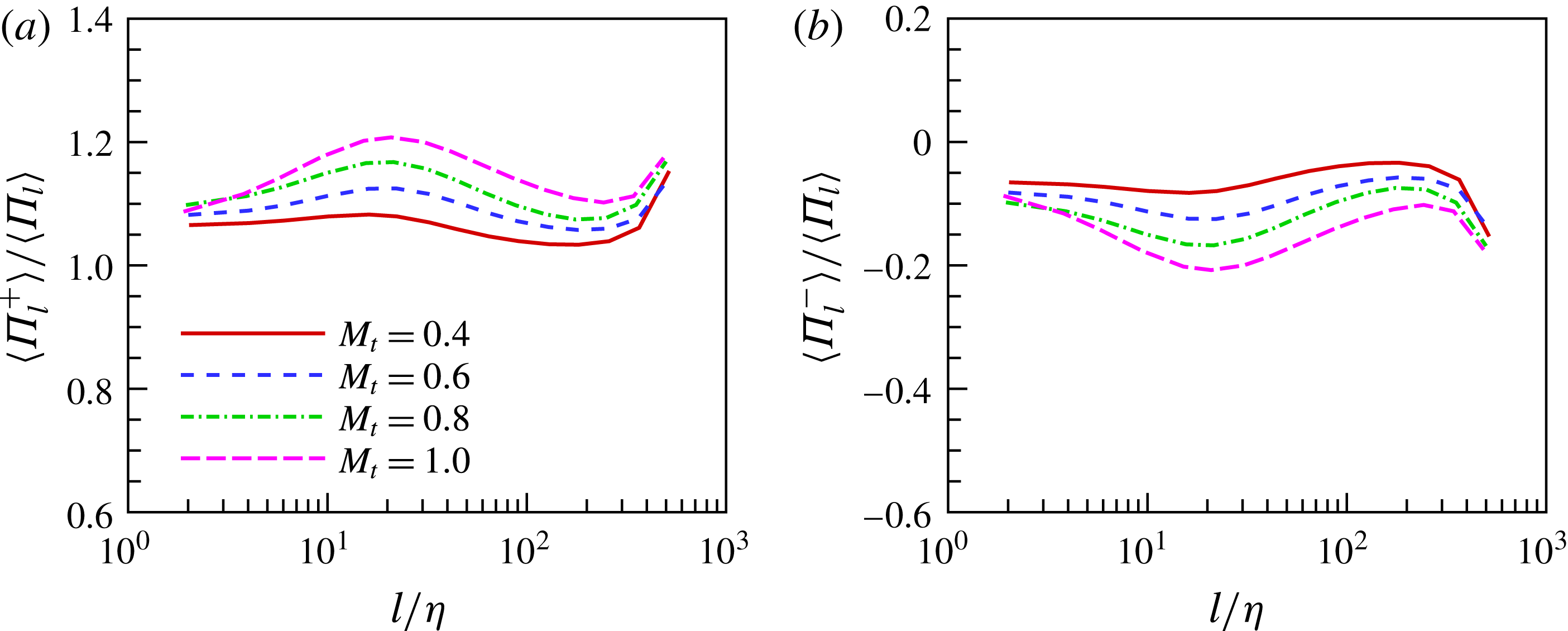
. We plot normalized ensemble averages of the positive and negative components of SGS flux at turbulent Mach numbers
 $M_{t}=0.4,0.6,0.8,1.0$
in figure 6. We see that as turbulent Mach number increases, both magnitudes of
 $\langle \unicode[STIX]{x1D6F1}_{l}^{+}\rangle /\langle \unicode[STIX]{x1D6F1}_{l}\rangle$
and
 $\langle \unicode[STIX]{x1D6F1}_{l}^{-}\rangle /\langle \unicode[STIX]{x1D6F1}_{l}\rangle$
become larger, demonstrating the significant effect of compressibility on the SGS energy transfer. Particularly, the SGS backscatter of kinetic energy becomes more important at higher turbulent Mach number.
Normalized ensemble average of the positive and negative components of SGS flux at turbulent Mach numbers
 $M_{t}=0.4,0.6,0.8,1.0$
.

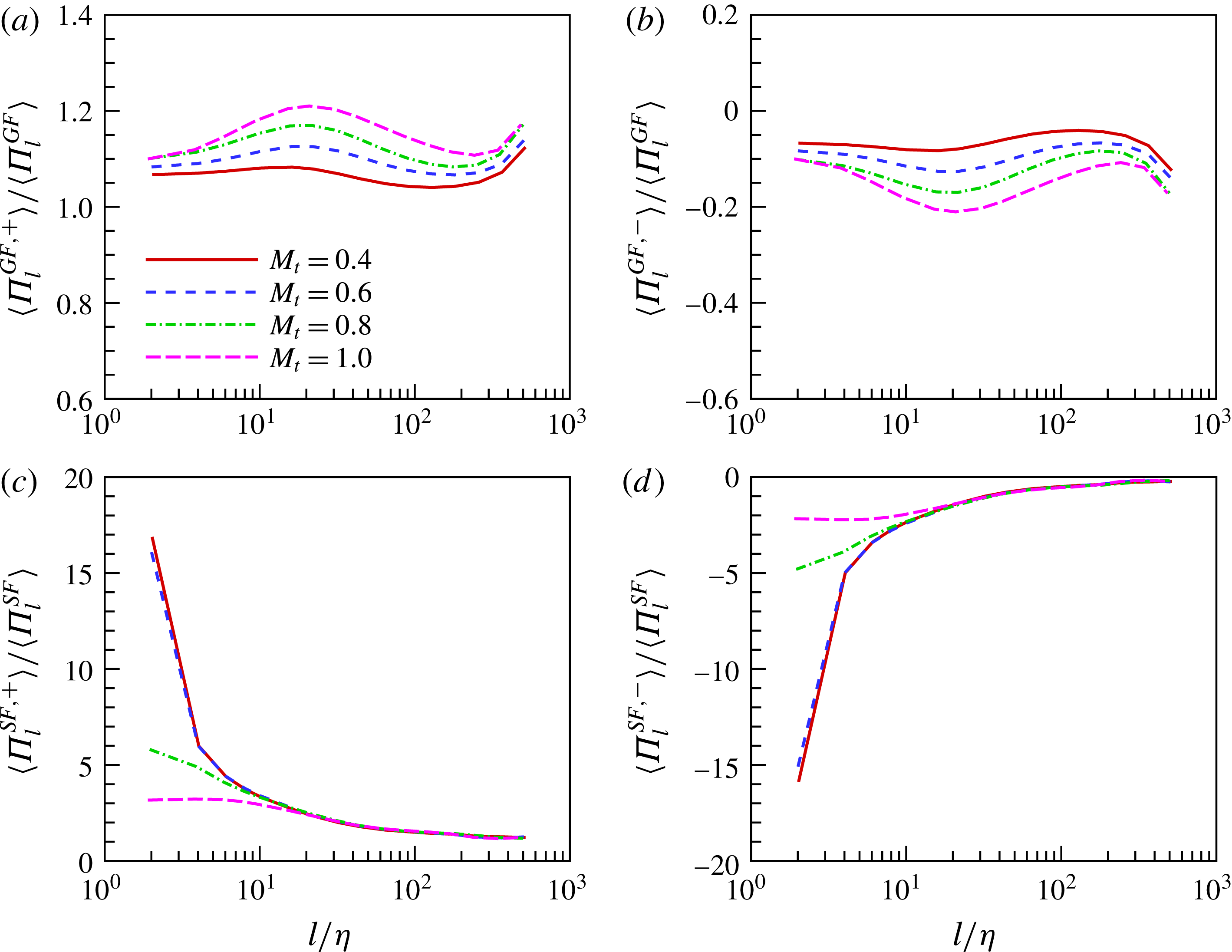
In figure 7, we plot the normalized ensemble average of the positive and negative components of SGS flux by using the Gaussian filter and the sharp spectral filter. The behaviours of
 $\langle \unicode[STIX]{x1D6F1}_{l}^{GF,+}\rangle /\langle \unicode[STIX]{x1D6F1}_{l}^{GF}\rangle$
and
 $\langle \unicode[STIX]{x1D6F1}_{l}^{GF,-}\rangle /\langle \unicode[STIX]{x1D6F1}_{l}^{GF}\rangle$
are almost the same as those of
 $\langle \unicode[STIX]{x1D6F1}_{l}^{+}\rangle /\langle \unicode[STIX]{x1D6F1}_{l}\rangle$
and
 $\langle \unicode[STIX]{x1D6F1}_{l}^{-}\rangle /\langle \unicode[STIX]{x1D6F1}_{l}\rangle$
. The magnitude of negative component of SGS flux is much smaller than its positive counterpart for the top-hat filter and Gaussian filter. In contrast, the magnitudes of
 $\langle \unicode[STIX]{x1D6F1}_{l}^{SF,+}\rangle /\langle \unicode[STIX]{x1D6F1}_{l}^{SF}\rangle$
and
 $\langle \unicode[STIX]{x1D6F1}_{l}^{SF,-}\rangle /\langle \unicode[STIX]{x1D6F1}_{l}^{SF}\rangle$
are nearly equal to each other and are much larger than 1, particularly, at small scales
 $l/\unicode[STIX]{x1D702}\leqslant 10$
, which is consistent with the fact that the PDF of
 $\unicode[STIX]{x1D6F1}_{l}^{SF}/\unicode[STIX]{x1D716}_{T}$
is nearly symmetric. The observation is in agreement with the previous study that roughly
 $50\,\%$
of the grid points were experiencing backscatter when a sharp spectral filter was used in incompressible turbulence (Lee et al.
Reference Lee, Lele and Moin1991).
Normalized ensemble average of the positive and negative components of SGS flux by using the Gaussian filter and the sharp spectral filter.

Since the sharp spectral filter is not positive in physical space, a filtered density by the sharp spectral filter can have negative values in space, which would violate fundamental conservation laws (Aluie Reference Aluie2013). Thus, the sharp spectral filter is rarely applied in the study of compressible turbulence. Different from the sharp spectral filter, the top-hat filter and the Gaussian filter are positive in physical space, and can be interpreted as local space average. It is reasonable that the statistics of the SGS flux of kinetic energy in physical space by the sharp spectral filter can be different from those by the top-hat filter and the Gaussian filter. Our numerical results on the kinetic energy transfer by the top-hat filter and the Gaussian filter are consistent with the theoretical analysis by Aluie (Reference Aluie2013). In contrast to the situation of compressible turbulence, both sharp spectral filter and smooth filters are popular in the analysis of energy transfer in incompressible turbulence. Aluie & Eyink (Reference Aluie and Eyink2009) pointed out that individual Fourier modes have no physical significance. Summation over logarithmic wavenumber bands is necessary to a physical description of turbulent cascade which is resolved both in scale and in space. The log-banded energy transfer by the sharp spectral filter was shown to exhibit the scale locality, which is similar to the analysis of energy transfer by smooth filters (Domaradzki & Carati Reference Domaradzki and Carati2007a ,Reference Domaradzki and Carati b ; Aluie & Eyink Reference Aluie and Eyink2009; Eyink & Aluie Reference Eyink and Aluie2009).
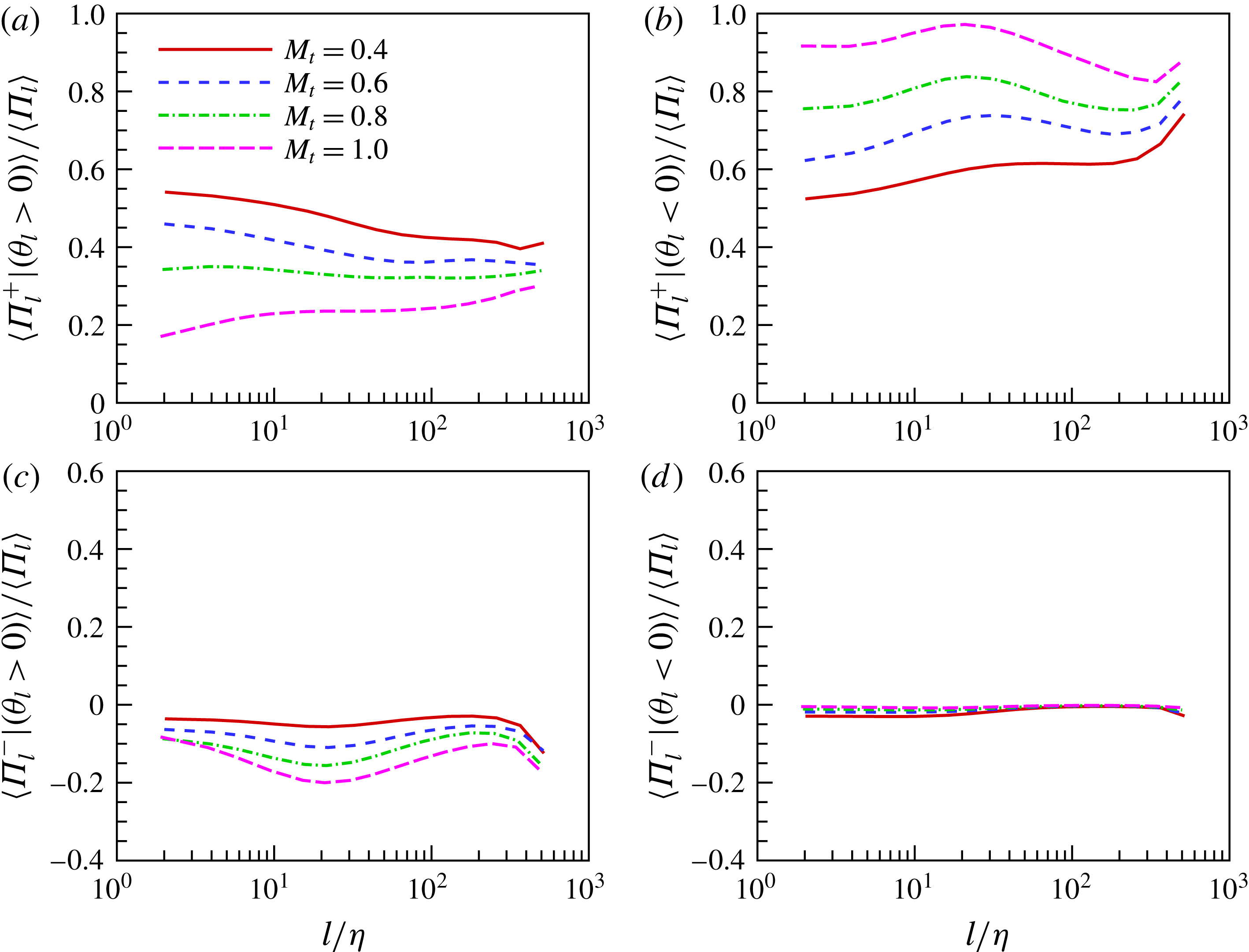
Conditional average of the positive and negative components of SGS flux at turbulent Mach numbers
 $M_{t}=0.4,0.6,0.8,1.0$
.

5.2 Effect of velocity divergence on SGS flux of kinetic energy
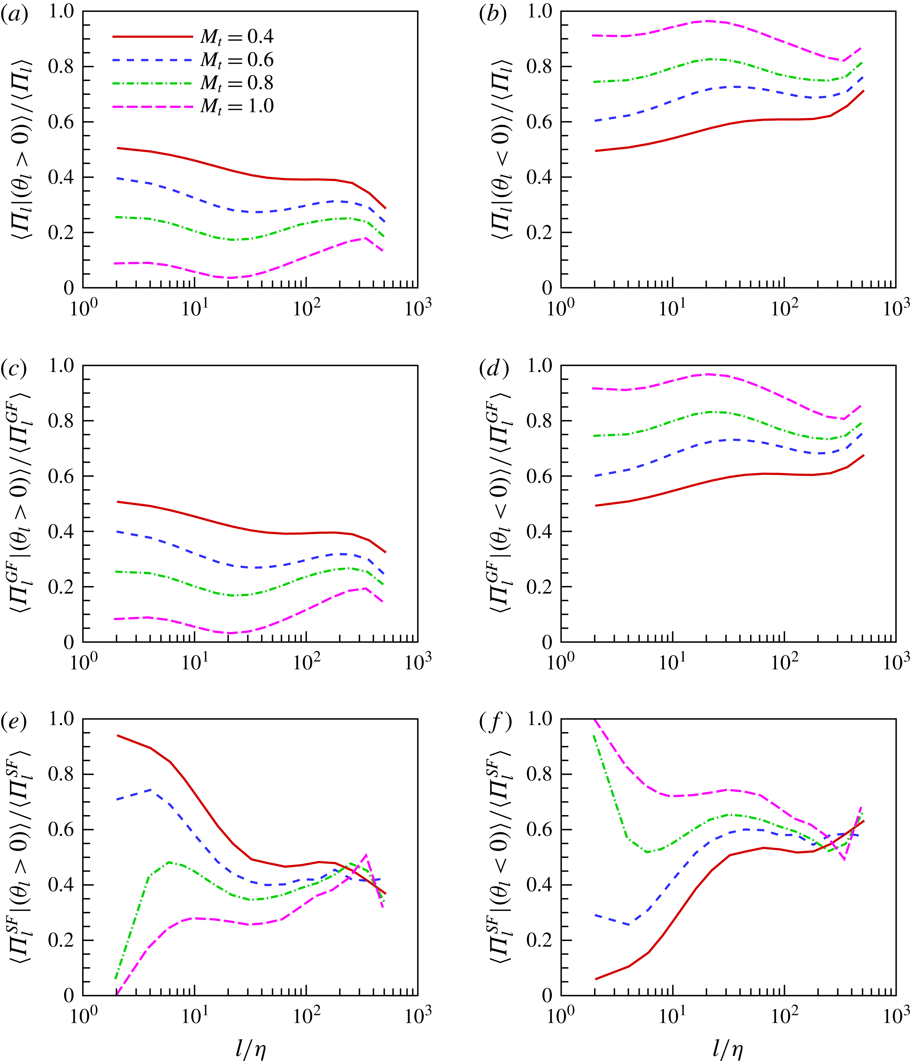
In order to study the effect of compression and expansion motions on the SGS kinetic energy transfer, we consider the following conditional average of the positive and negative components of SGS flux:
 $\langle \unicode[STIX]{x1D6F1}_{l}^{+}|\unicode[STIX]{x1D703}_{l}>0\rangle$
,
 $\langle \unicode[STIX]{x1D6F1}_{l}^{+}|\unicode[STIX]{x1D703}_{l}<0\rangle$
,
 $\langle \unicode[STIX]{x1D6F1}_{l}^{-}|\unicode[STIX]{x1D703}_{l}>0\rangle$
and
 $\langle \unicode[STIX]{x1D6F1}_{l}^{-}|\unicode[STIX]{x1D703}_{l}<0\rangle$
, where the filtered velocity divergence is
 $\unicode[STIX]{x1D703}_{l}=\unicode[STIX]{x1D735}\boldsymbol{\cdot }\widetilde{\boldsymbol{u}}$
. We plot the conditional average of the positive and negative components of SGS flux at turbulent Mach numbers
 $M_{t}=0.4,0.6,0.8,1.0$
in figure 8. We find that as turbulent Mach number increases from
 $0.4$
to
 $1.0$
,
 $\langle \unicode[STIX]{x1D6F1}_{l}^{+}|\unicode[STIX]{x1D703}_{l}>0\rangle /\langle \unicode[STIX]{x1D6F1}_{l}\rangle$
decreases, while the magnitude of
 $\langle \unicode[STIX]{x1D6F1}_{l}^{-}|\unicode[STIX]{x1D703}_{l}>0\rangle /\langle \unicode[STIX]{x1D6F1}_{l}\rangle$
increases. Thus, at higher turbulent Mach number, expansion motions are more likely to suppress the direct SGS flux of kinetic energy from large scales to small scales, and enhance the reverse SGS flux of kinetic energy from small scales to large scales. We also observe that as turbulent Mach number increases from
 $0.4$
to
 $1.0$
,
 $\langle \unicode[STIX]{x1D6F1}_{l}^{+}|\unicode[STIX]{x1D703}_{l}<0\rangle /\langle \unicode[STIX]{x1D6F1}_{l}\rangle$
increases, indicating that compression motions have a tendency to enhance the direct SGS flux of kinetic energy from large scales to small scales. The reverse SGS flux in compression regions is negligibly small for all turbulent Mach numbers in our simulations.
Conditional average of SGS flux by using the top-hat filter, the Gaussian filter and the sharp spectral filter: (a,b) top-hat filter; (c,d) Gaussian filter (GF); (e,f) sharp spectral filter (SF).

In figure 9, we plot the conditional average of the SGS flux by using the top-hat filter, the Gaussian filter and the sharp spectral filter. We find that both
 $\langle \unicode[STIX]{x1D6F1}_{l}|\unicode[STIX]{x1D703}_{l}>0\rangle /\langle \unicode[STIX]{x1D6F1}_{l}\rangle$
and
 $\langle \unicode[STIX]{x1D6F1}_{l}|\unicode[STIX]{x1D703}_{l}<0\rangle /\langle \unicode[STIX]{x1D6F1}_{l}\rangle$
are close to
 $0.5$
at
 $M_{t}=0.4$
. As turbulent Mach number increases from
 $0.4$
to
 $1.0$
,
 $\langle \unicode[STIX]{x1D6F1}_{l}|\unicode[STIX]{x1D703}_{l}>0\rangle /\langle \unicode[STIX]{x1D6F1}_{l}\rangle$
decreases, while
 $\langle \unicode[STIX]{x1D6F1}_{l}|\unicode[STIX]{x1D703}_{l}<0\rangle /\langle \unicode[STIX]{x1D6F1}_{l}\rangle$
increases.
 $\langle \unicode[STIX]{x1D6F1}_{l}|\unicode[STIX]{x1D703}_{l}>0\rangle /\langle \unicode[STIX]{x1D6F1}_{l}\rangle$
becomes much smaller than
 $\langle \unicode[STIX]{x1D6F1}_{l}|\unicode[STIX]{x1D703}_{l}<0\rangle /\langle \unicode[STIX]{x1D6F1}_{l}\rangle$
at
 $M_{t}=1.0$
. The results from the Gaussian filter are almost identical to those from the top-hat filter. In contrast, the results from the sharp spectral filter are quantitatively different. Both
 $\langle \unicode[STIX]{x1D6F1}_{l}^{SF}|\unicode[STIX]{x1D703}_{l}>0\rangle /\langle \unicode[STIX]{x1D6F1}_{l}^{SF}\rangle$
and
 $\langle \unicode[STIX]{x1D6F1}_{l}^{SF}|\unicode[STIX]{x1D703}_{l}<0\rangle /\langle \unicode[STIX]{x1D6F1}_{l}^{SF}\rangle$
are very sensitive to the change of turbulent Mach number at small scales
 $l/\unicode[STIX]{x1D702}\leqslant 10$
. It is shown that for small scales
 $l/\unicode[STIX]{x1D702}\leqslant 10$
,
 $\langle \unicode[STIX]{x1D6F1}_{l}^{SF}|\unicode[STIX]{x1D703}_{l}>0\rangle /\langle \unicode[STIX]{x1D6F1}_{l}^{SF}\rangle$
is close to
 $1.0$
at
 $M_{t}=0.4$
, but it is close to
 $0$
at
 $M_{t}=1.0$
. It is worth noting that compression regions have a major contribution to the net SGS flux of kinetic energy at high turbulent Mach number
 $M_{t}=1.0$
for the three types of filters.
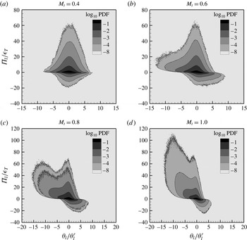
Joint PDF of
 $\unicode[STIX]{x1D6F1}_{l}/\unicode[STIX]{x1D716}_{T}$
and
 $\unicode[STIX]{x1D703}_{l}/\unicode[STIX]{x1D703}_{l}^{\prime }$
for the filter width
 $l/\unicode[STIX]{x1D702}=16$
at turbulent Mach numbers
 $M_{t}=0.4,0.6,0.8,1.0$
.

We plot the joint PDF of the normalized SGS kinetic energy flux
 $\unicode[STIX]{x1D6F1}_{l}/\unicode[STIX]{x1D716}_{T}$
and the normalized filtered velocity divergence
 $\unicode[STIX]{x1D703}_{l}/\unicode[STIX]{x1D703}_{l}^{\prime }$
for the filter width
 $l/\unicode[STIX]{x1D702}=16$
at turbulent Mach numbers
 $M_{t}=0.4,0.6,0.8,1.0$
in figure 10. At turbulent Mach number
 $M_{t}=0.4$
, the shape of the joint PDF is nearly symmetric with respect to the line
 $\unicode[STIX]{x1D703}_{l}/\unicode[STIX]{x1D703}_{l}^{\prime }=0$
, indicating that the contributions of compression regions and expansion regions to the SGS flux are nearly equal to each other. As the turbulent Mach number increases from
 $0.4$
to
 $1.0$
, the fractions of the second and fourth quadrants of the joint PDF become larger, while the fractions of the first and third quadrants become smaller. For
 $M_{t}\geqslant 0.6$
, compression regions have a major contribution to the direct SGS flux of kinetic energy, while expansion regions have a major contribution to the reverse SGS flux of kinetic energy. The observations are consistent with a previous result that backscatter occurs primarily in regions undergoing volumetric expansion in a reacting turbulent mixing layers (O’Brien et al.
Reference O’Brien, Urzay, Ihme, Moin and Saghafian2014). At
 $M_{t}=1.0$
, the second quadrant of the joint PDF predominates over other three quadrants, indicating that the occurrence of strong compression associated with the shocklet structure greatly enhances the direct SGS flux of kinetic energy from large scales to small scales.
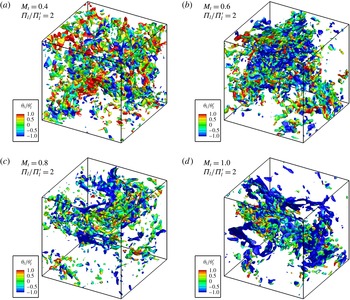
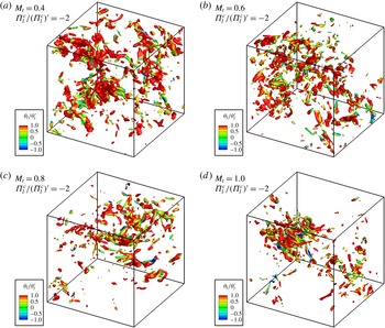
Figure 11 displays the isosurfaces of SGS flux at
 $\unicode[STIX]{x1D6F1}_{l}/\unicode[STIX]{x1D6F1}_{l}^{\prime }=2$
for the filter width
 $l/\unicode[STIX]{x1D702}=16$
, at turbulent Mach numbers
 $M_{t}=0.4,0.6,0.8,1.0$
. The isosurfaces are coloured based on the normalized filtered velocity divergence
 $\unicode[STIX]{x1D703}_{l}/\unicode[STIX]{x1D703}_{l}^{\prime }$
. At
 $M_{t}=0.4$
, the isosurfaces
 $\unicode[STIX]{x1D6F1}_{l}/\unicode[STIX]{x1D6F1}_{l}^{\prime }=2$
can be identified as blob-like structures which are nearly uniformly distributed over the whole flow field. In addition, the fractions of expansion and compression regions on the isosurfaces are nearly equal to each other at
 $M_{t}=0.4$
. As turbulent Mach number increases, part of isosurfaces become sheet-like, associated with strong compression motions, which can be attributed to the generation of shocklets at moderate and high turbulent Mach numbers
 $M_{t}\geqslant 0.6$
. The fraction of sheet-like structures of the isosurfaces increases with the increase of turbulent Mach number, since more stronger shocklets can be generated at a higher Mach number (Wang et al.
Reference Wang, Gotoh and Watanabe2017b
; Wang, Gotoh & Watanabe Reference Wang, Gotoh and Watanabe2017c
). At
 $M_{t}=1.0$
, most of the isosurfaces
 $\unicode[STIX]{x1D6F1}_{l}/\unicode[STIX]{x1D6F1}_{l}^{\prime }=2$
become sheet-like and exhibit high compression
 $\unicode[STIX]{x1D703}_{l}/\unicode[STIX]{x1D703}_{l}^{\prime }<-1.0$
, demonstrating the significant effect of shocklets. Moreover, the isosurfaces
 $\unicode[STIX]{x1D6F1}_{l}/\unicode[STIX]{x1D6F1}_{l}^{\prime }=2$
are no longer uniformly distributed and exhibit the spatial intermittency at
 $M_{t}=1.0$
.
Isosurfaces of SGS flux at
 $\unicode[STIX]{x1D6F1}_{l}/\unicode[STIX]{x1D6F1}_{l}^{\prime }=2$
for the filter width
 $l/\unicode[STIX]{x1D702}=16$
, at turbulent Mach numbers
 $M_{t}=0.4,0.6,0.8,1.0$
.

We plot the isosurfaces of SGS flux at
 $\unicode[STIX]{x1D6F1}_{l}/\unicode[STIX]{x1D6F1}_{l}^{\prime }=-0.5$
for the filter width
 $l/\unicode[STIX]{x1D702}=16$
, at turbulent Mach numbers
 $M_{t}=0.4,0.6,0.8,1.0$
in figure 12. The isosurfaces are coloured based on the normalized filtered velocity divergence
 $\unicode[STIX]{x1D703}_{l}/\unicode[STIX]{x1D703}_{l}^{\prime }$
. At
 $M_{t}=0.4$
, the isosurfaces
 $\unicode[STIX]{x1D6F1}_{l}/\unicode[STIX]{x1D6F1}_{l}^{\prime }=-0.5$
are also blob-like, but are more sparse, with smaller length scales in the flow field, as compared with the isosurfaces
 $\unicode[STIX]{x1D6F1}_{l}/\unicode[STIX]{x1D6F1}_{l}^{\prime }=2$
, revealing the fact that the reverse SGS flux of kinetic energy is much weaker than the direct SGS flux of kinetic energy. The isosurfaces
 $\unicode[STIX]{x1D6F1}_{l}/\unicode[STIX]{x1D6F1}_{l}^{\prime }=-0.5$
are nearly equally distributed in compression regions and expansion regions at
 $M_{t}=0.4$
. As turbulent Mach number increases, the isosurfaces
 $\unicode[STIX]{x1D6F1}_{l}/\unicode[STIX]{x1D6F1}_{l}^{\prime }=-0.5$
tend to exhibit larger length scales with stronger expansion motions. Thus, expansion motions can substantially enhance the reverse SGS flux of kinetic energy at moderate and high turbulent Mach numbers
 $M_{t}\geqslant 0.6$
. At
 $M_{t}=1.0$
, most of isosurfaces
 $\unicode[STIX]{x1D6F1}_{l}/\unicode[STIX]{x1D6F1}_{l}^{\prime }=-0.5$
are distributed in strong expansion regions
 $\unicode[STIX]{x1D703}_{l}/\unicode[STIX]{x1D703}_{l}^{\prime }>1.0$
, and exhibit similar spatial intermittency as compared with the isosurfaces
 $\unicode[STIX]{x1D6F1}_{l}/\unicode[STIX]{x1D6F1}_{l}^{\prime }=2.0$
. We infer that the regions of strong reverse flux of kinetic energy associated with strong expansion motions are usually close to some regions of strong direct flux of kinetic energy associated with strong compression motions. The observations are consistent with the fact that expansion regions can be identified just downstream of shocklets in compressible isotropic turbulence (Wang et al.
Reference Wang, Shi, Wang, Xiao, He and Chen2011).
Isosurfaces of SGS flux at
 $\unicode[STIX]{x1D6F1}_{l}/\unicode[STIX]{x1D6F1}_{l}^{\prime }=-0.5$
for the filter width
 $l/\unicode[STIX]{x1D702}=16$
, at turbulent Mach numbers
 $M_{t}=0.4,0.6,0.8,1.0$
.

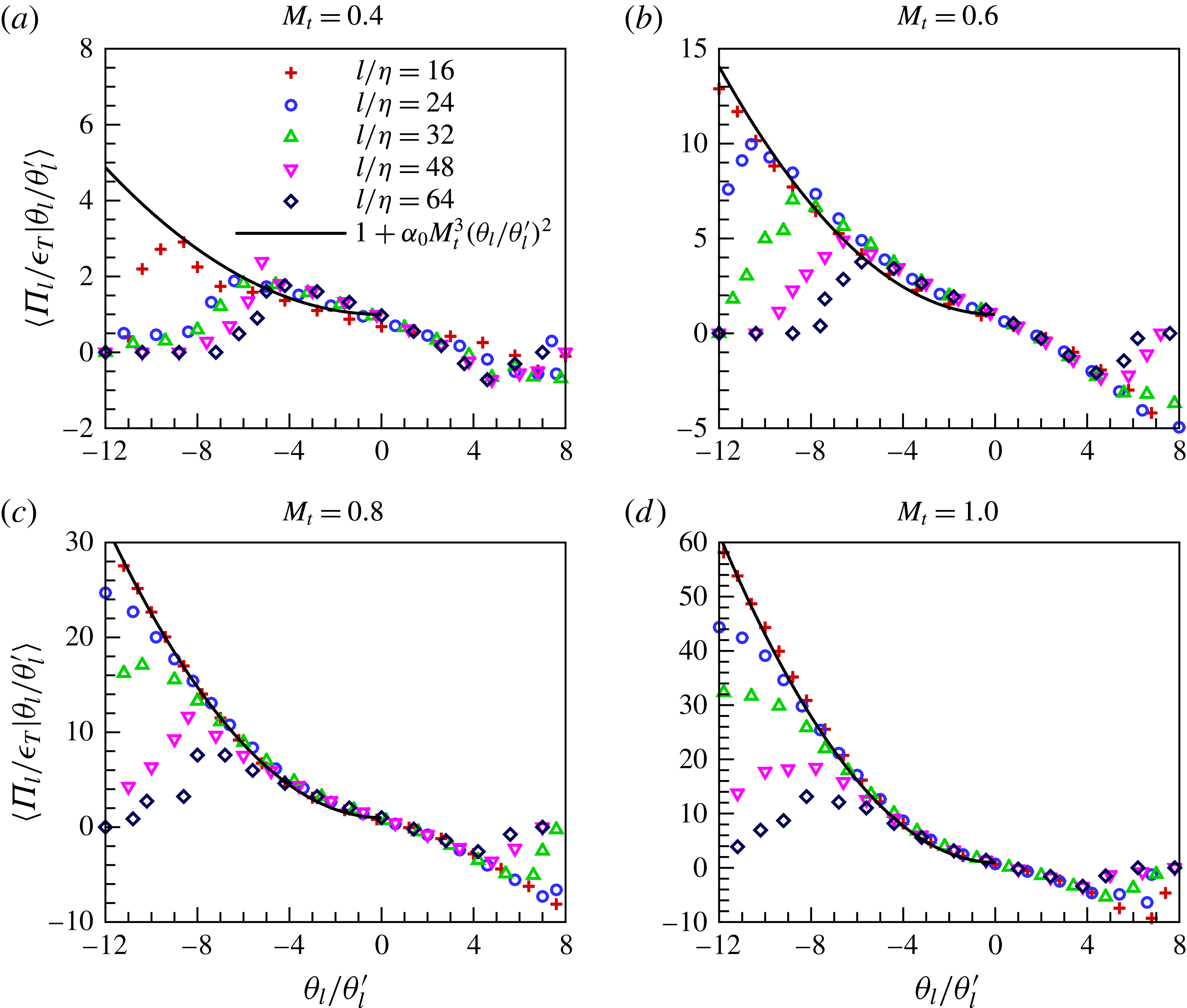
Average of normalized SGS flux
 $\unicode[STIX]{x1D6F1}_{l}/\unicode[STIX]{x1D716}_{T}$
conditioned on the normalized filtered velocity divergence
 $\unicode[STIX]{x1D703}_{l}/\unicode[STIX]{x1D703}_{l}^{\prime }$
for different filter widths
 $l/\unicode[STIX]{x1D702}=16,24,32,48,64$
at turbulent Mach numbers
 $M_{t}=0.4,0.6,0.8,1.0$
.

We plot the average of normalized SGS flux
 $\unicode[STIX]{x1D6F1}_{l}/\unicode[STIX]{x1D716}_{T}$
conditioned on the normalized filtered velocity divergence
 $\unicode[STIX]{x1D703}_{l}/\unicode[STIX]{x1D703}_{l}^{\prime }$
for different filter widths
 $l/\unicode[STIX]{x1D702}=16,24,32,48,64$
at turbulent Mach numbers
 $M_{t}=0.4,0.6,0.8,1.0$
in figure 13. We find that the conditional average of SGS flux is nearly independent of filter width
 $l/\unicode[STIX]{x1D702}$
, for
 $16\leqslant l/\unicode[STIX]{x1D702}\leqslant 64$
at moderate and high turbulent Mach numbers
 $M_{t}\geqslant 0.6$
in our numerical simulations. Due to the lack of samples, the data are quite scattered when the magnitude of velocity divergence
 $\unicode[STIX]{x1D703}_{l}/\unicode[STIX]{x1D703}_{l}^{\prime }$
and the filter width
 $l/\unicode[STIX]{x1D702}$
are large. We show again that strong compression motions induce strong direct SGS flux of kinetic energy, while strong expansion motions induce strong reverse SGS flux of kinetic energy, at turbulent Mach numbers
 $0.6\leqslant M_{t}\leqslant 1.0$
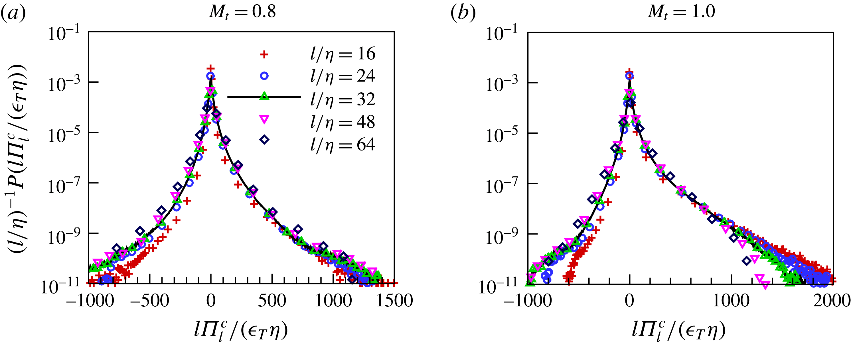
. Moreover, we propose a simple model for the conditional average of SGS flux in compression regions
 $\unicode[STIX]{x1D703}_{l}\leqslant 0$
:
 $$\begin{eqnarray}\displaystyle & \displaystyle \left\langle \unicode[STIX]{x1D6F1}_{l}/\unicode[STIX]{x1D716}_{T}\big|\unicode[STIX]{x1D703}_{l}/\unicode[STIX]{x1D703}_{l}^{\prime }\right\rangle =1+\unicode[STIX]{x1D6FC}_{0}M_{t}^{3}\left(\unicode[STIX]{x1D703}_{l}/\unicode[STIX]{x1D703}_{l}^{\prime }\right)^{2}, & \displaystyle\end{eqnarray}$$
where,
 $\unicode[STIX]{x1D6FC}_{0}=0.42$
. The numerical results on the conditional SGS flux are in good agreement with (5.1) at turbulent Mach numbers
 $M_{t}=0.6,0.8,1.0$
. It is worth noting that the local viscous dissipation of kinetic energy increases linearly with the square of filtered velocity divergence in shock regions (strong compression regions). Equation (5.1) gives a similar relation: SGS flux of kinetic energy increases linearly with the square of filtered velocity divergence in shock regions. The observations are consistent with the kinetic-energy-cascade scenario: the kinetic energy is usually generated at the integral length scale, transferred from large scales to small scales and dissipated at the Kolmogorov length scale. In the inertial range between the integral length scale and Kolmogorov length scale, the inter-scale transfer of kinetic energy nearly exhibits the scale-invariant property, such as the fact that the ensemble average of SGS flux is nearly constant. Here, we show that the
 $\unicode[STIX]{x1D703}_{l}$
-square scaling of conditional average of SGS flux is also nearly scale invariant in strong compression regions during the kinetic energy cascade in solenoidally forced compressible isotropic turbulence. The observations are similar to those in a previous numerical simulation of compressible isotropic turbulence applying a large-scale force to both the solenoidal and compressive components of the velocity field (Wang et al.
Reference Wang, Yang, Shi, Xiao, He and Chen2013).
Average of normalized SGS flux
 $\unicode[STIX]{x1D6F1}_{l}/\unicode[STIX]{x1D716}_{T}$
conditioned on the normalized filtered velocity divergence
 $\unicode[STIX]{x1D703}_{l}/\unicode[STIX]{x1D703}_{l}^{\prime }$
for different filter widths
 $l/\unicode[STIX]{x1D702}=16,24,32,48,64$
in expansion regions. Here,
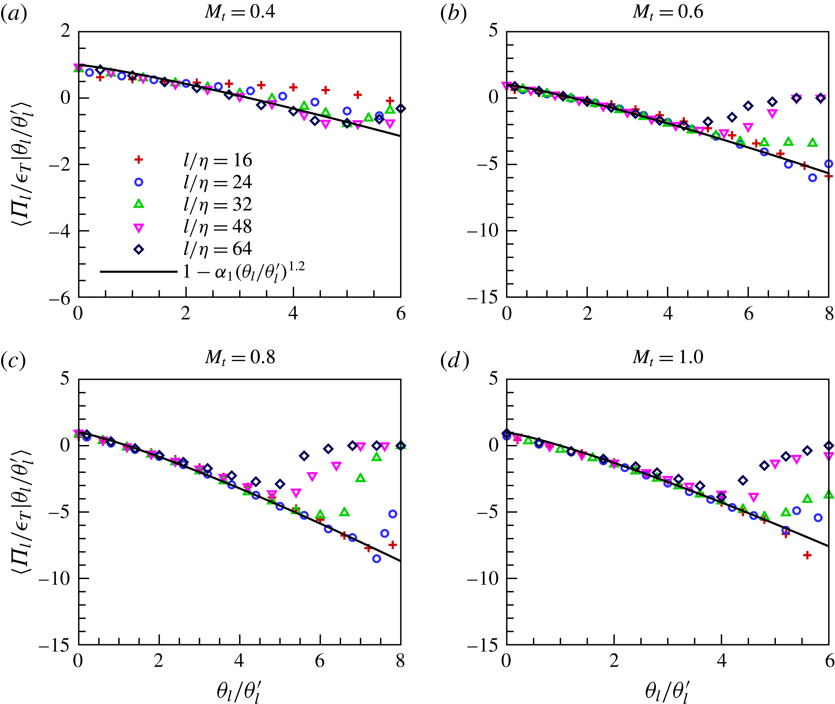
 $\unicode[STIX]{x1D6FC}_{1}=0.25,0.55,0.8,1.0$
for turbulent Mach numbers
 $M_{t}=0.4,0.6,0.8,1.0$
, respectively.

In figure 14, we plot the conditional average of normalized SGS flux
 $\unicode[STIX]{x1D6F1}_{l}/\unicode[STIX]{x1D716}_{T}$
for different filter widths
 $l/\unicode[STIX]{x1D702}=16,24,32,48,64$
in expansion regions
 $\unicode[STIX]{x1D703}_{l}\geqslant 0$
. We propose a simple model for the conditional average of the SGS flux in expansion regions
 $\unicode[STIX]{x1D703}_{l}\geqslant 0$
:
 $$\begin{eqnarray}\displaystyle & \displaystyle \left\langle \unicode[STIX]{x1D6F1}_{l}/\unicode[STIX]{x1D716}_{T}\big|\unicode[STIX]{x1D703}_{l}/\unicode[STIX]{x1D703}_{l}^{\prime }\right\rangle =1-\unicode[STIX]{x1D6FC}_{1}\left(\unicode[STIX]{x1D703}_{l}/\unicode[STIX]{x1D703}_{l}^{\prime }\right)^{1.2}, & \displaystyle\end{eqnarray}$$
where,
 $\unicode[STIX]{x1D6FC}_{1}=0.25,0.55,0.8,1.0$
for turbulent Mach numbers
 $M_{t}=0.4,0.6,0.8,1.0$
, respectively. The numerical results on the conditional SGS flux are in good agreement with (5.2) at turbulent Mach numbers
 $M_{t}=0.6,0.8,1.0$
. The model demonstrates that strong expansion motions induce a strong reverse SGS flux of kinetic energy at turbulent Mach numbers
 $0.6\leqslant M_{t}\leqslant 1.0$
. In addition, for a given
 $\unicode[STIX]{x1D703}_{l}$
in strong expansion regions, the magnitude of conditional average of
 $\unicode[STIX]{x1D6F1}_{l}/\unicode[STIX]{x1D716}_{T}$
increases with the increase of turbulent Mach number, giving rise to stronger reverse SGS flux of kinetic energy at higher turbulent Mach number. We emphasize that the magnitude of conditional average of normalized SGS flux
 $\unicode[STIX]{x1D6F1}_{l}/\unicode[STIX]{x1D716}_{T}$
in strong compression regions is much higher than that in strong expansion regions, which is consistent with a general physical insight that the flow statistics in strong compression regions are more intermittent than that in strong expansion regions for compressible turbulence at high turbulent Mach number (Wang et al.
Reference Wang, Shi, Wang, Xiao, He and Chen2012b
, Reference Wang, Gotoh and Watanabe2017b
,Reference Wang, Gotoh and Watanabe
c
).
Average of
 $\unicode[STIX]{x1D6FD}_{l}$
conditioned on the normalized filtered velocity divergence
 $\unicode[STIX]{x1D703}_{l}/\unicode[STIX]{x1D703}_{l}^{\prime }$
for different filter widths
 $l/\unicode[STIX]{x1D702}=16,24,32,48,64$
at turbulent Mach numbers
 $M_{t}=0.4,0.6,0.8,1.0$
.

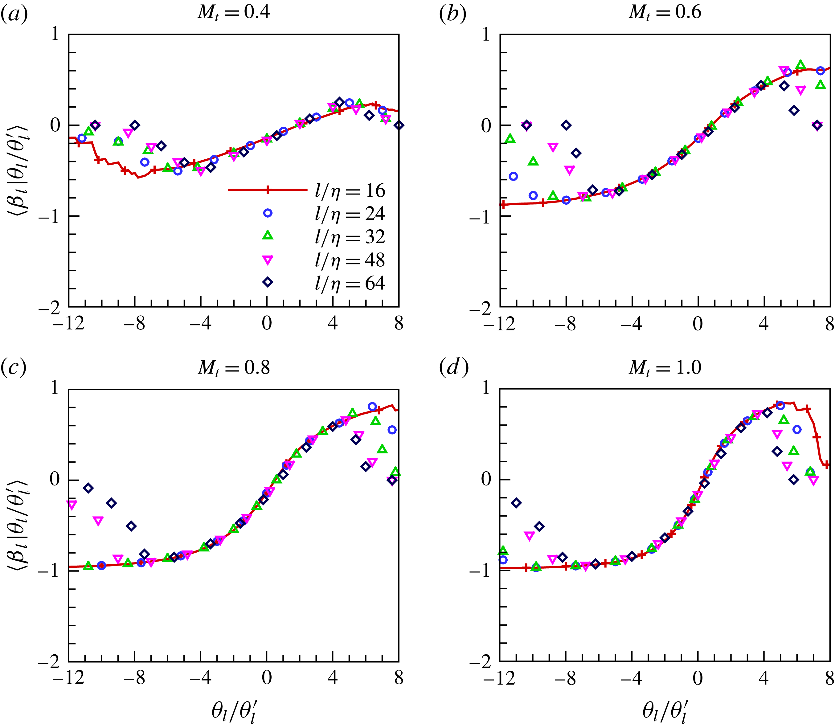
In order to investigate the relation between the large-scale strain and the SGS stress, we define the variable
 $\unicode[STIX]{x1D6FD}_{l}$
as follows:
 $$\begin{eqnarray}\displaystyle & \displaystyle \unicode[STIX]{x1D6FD}_{l}\equiv \frac{\widetilde{\unicode[STIX]{x1D70F}}_{ij}\widetilde{\unicode[STIX]{x1D61A}}_{ij}}{|\widetilde{\boldsymbol{\unicode[STIX]{x1D70F}}}||\widetilde{\unicode[STIX]{x1D64E}}|}, & \displaystyle\end{eqnarray}$$
where,
 $|\widetilde{\boldsymbol{\unicode[STIX]{x1D70F}}}|=\sqrt{\widetilde{\unicode[STIX]{x1D70F}}_{ij}\widetilde{\unicode[STIX]{x1D70F}}_{ij}}$
and
 $|\widetilde{\unicode[STIX]{x1D64E}}|=\sqrt{\widetilde{\unicode[STIX]{x1D61A}}_{ij}\widetilde{\unicode[STIX]{x1D61A}}_{ij}}$
. We plot the average of
 $\unicode[STIX]{x1D6FD}_{l}$
conditioned on the normalized filtered velocity divergence
 $\unicode[STIX]{x1D703}_{l}/\unicode[STIX]{x1D703}_{l}^{\prime }$
for different filter widths
 $l/\unicode[STIX]{x1D702}=16,24,32,48,64$
at turbulent Mach numbers
 $M_{t}=0.4,0.6,0.8,1.0$
in figure 15. At moderate and high turbulent Mach numbers
 $0.6\leqslant M_{t}\leqslant 1.0$
, the conditional averages of
 $\unicode[STIX]{x1D6FD}_{l}$
collapse to a single curve for different filter widths in the range of
 $16\leqslant l/\unicode[STIX]{x1D702}\leqslant 64$
. In addition, we find that
 $\langle \unicode[STIX]{x1D6FD}_{l}|\unicode[STIX]{x1D703}_{l}/\unicode[STIX]{x1D703}_{l}^{\prime }\rangle$
is close to
 $-1$
for
 $\unicode[STIX]{x1D703}_{l}/\unicode[STIX]{x1D703}_{l}^{\prime }\leqslant -4$
, giving rise to the antiparallel alignment between the large-scale strain and the SGS stress in strong compression regions
 $\unicode[STIX]{x1D703}_{l}/\unicode[STIX]{x1D703}_{l}^{\prime }\leqslant -4$
. The antiparallel alignment maximize the SGS kinetic energy flux, demonstrating the high efficiency of inter-scale kinetic energy transfer induced by shocklets. We also present that
 $\langle \unicode[STIX]{x1D6FD}_{l}|\unicode[STIX]{x1D703}_{l}/\unicode[STIX]{x1D703}_{l}^{\prime }\rangle$
is positive for
 $\unicode[STIX]{x1D703}_{l}/\unicode[STIX]{x1D703}_{l}^{\prime }\geqslant 2$
, revealing the reverse SGS flux of kinetic energy from small scales to large scales in strong expansion regions (Wang et al.
Reference Wang, Yang, Shi, Xiao, He and Chen2013).
5.3 Helmholtz decomposition on SGS flux of kinetic energy
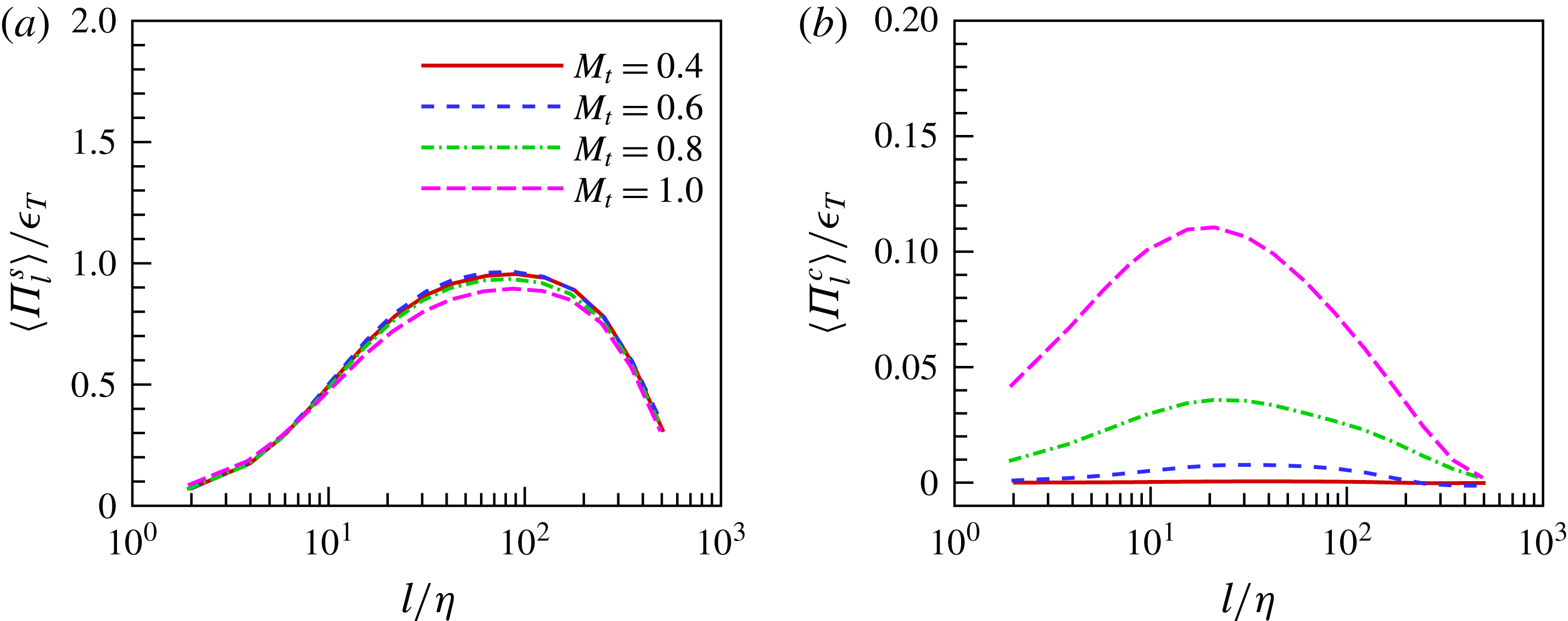
In figure 16, we depict the average of the solenoidal and compressible components of the SGS flux:
 $\langle \unicode[STIX]{x1D6F1}_{l}^{s}\rangle /\unicode[STIX]{x1D716}_{T}$
and
 $\langle \unicode[STIX]{x1D6F1}_{l}^{c}\rangle /\unicode[STIX]{x1D716}_{T}$
, at turbulent Mach numbers
 $M_{t}=0.4,0.6,0.8,1.0$
. The average solenoidal SGS flux
 $\langle \unicode[STIX]{x1D6F1}_{l}^{s}\rangle /\unicode[STIX]{x1D716}_{T}$
is nearly independent of turbulent Mach number in our numerical simulations.
 $\langle \unicode[STIX]{x1D6F1}_{l}^{s}\rangle /\unicode[STIX]{x1D716}_{T}$
is close to
 $1.0$
in the range of
 $30\leqslant l/\unicode[STIX]{x1D702}\leqslant 200$
. Consequently, the solenoidal SGS flux makes a major contribution to the net transfer of kinetic energy from large scales to small scales in the range of
 $30\leqslant l/\unicode[STIX]{x1D702}\leqslant 200$
. In contrast, the average compressible SGS flux
 $\langle \unicode[STIX]{x1D6F1}_{l}^{c}\rangle /\unicode[STIX]{x1D716}_{T}$
increases rapidly with the increase of turbulent Mach number, reflecting the significant effect of compressibility on the inter-scale transfer of compressible kinetic energy. At
 $M_{t}=1.0$
,
 $\langle \unicode[STIX]{x1D6F1}_{l}^{c}\rangle /\unicode[STIX]{x1D716}_{T}$
is close to
 $0.1$
in the range of
 $10\leqslant l/\unicode[STIX]{x1D702}\leqslant 40$
. Therefore, the contribution of compressible component to the net flux of kinetic energy is quite small as compared to its solenoidal counterpart.
Average of solenoidal and compressible components of the SGS flux: (a)
 $\langle \unicode[STIX]{x1D6F1}_{l}^{s}\rangle /\unicode[STIX]{x1D716}_{T}$
and (b)
 $\langle \unicode[STIX]{x1D6F1}_{l}^{c}\rangle /\unicode[STIX]{x1D716}_{T}$
.

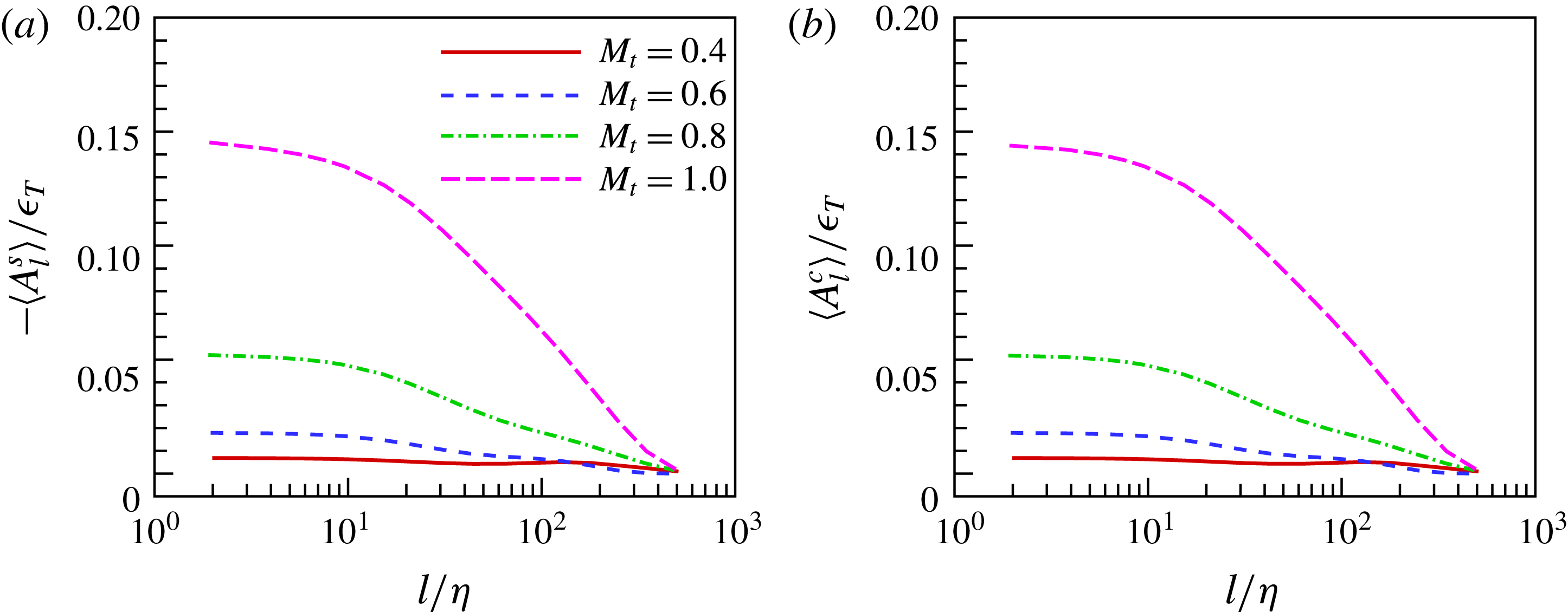
Figure 17 displays the average of solenoidal and compressible components of the nonlinear advection:
 $-\langle A_{l}^{s}\rangle /\unicode[STIX]{x1D716}_{T}$
and
 $\langle A_{l}^{c}\rangle /\unicode[STIX]{x1D716}_{T}$
, at turbulent Mach numbers
 $M_{t}=0.4,0.6,0.8,1.0$
. Both
 $-\langle A_{l}^{s}\rangle /\unicode[STIX]{x1D716}_{T}$
and
 $\langle A_{l}^{c}\rangle /\unicode[STIX]{x1D716}_{T}$
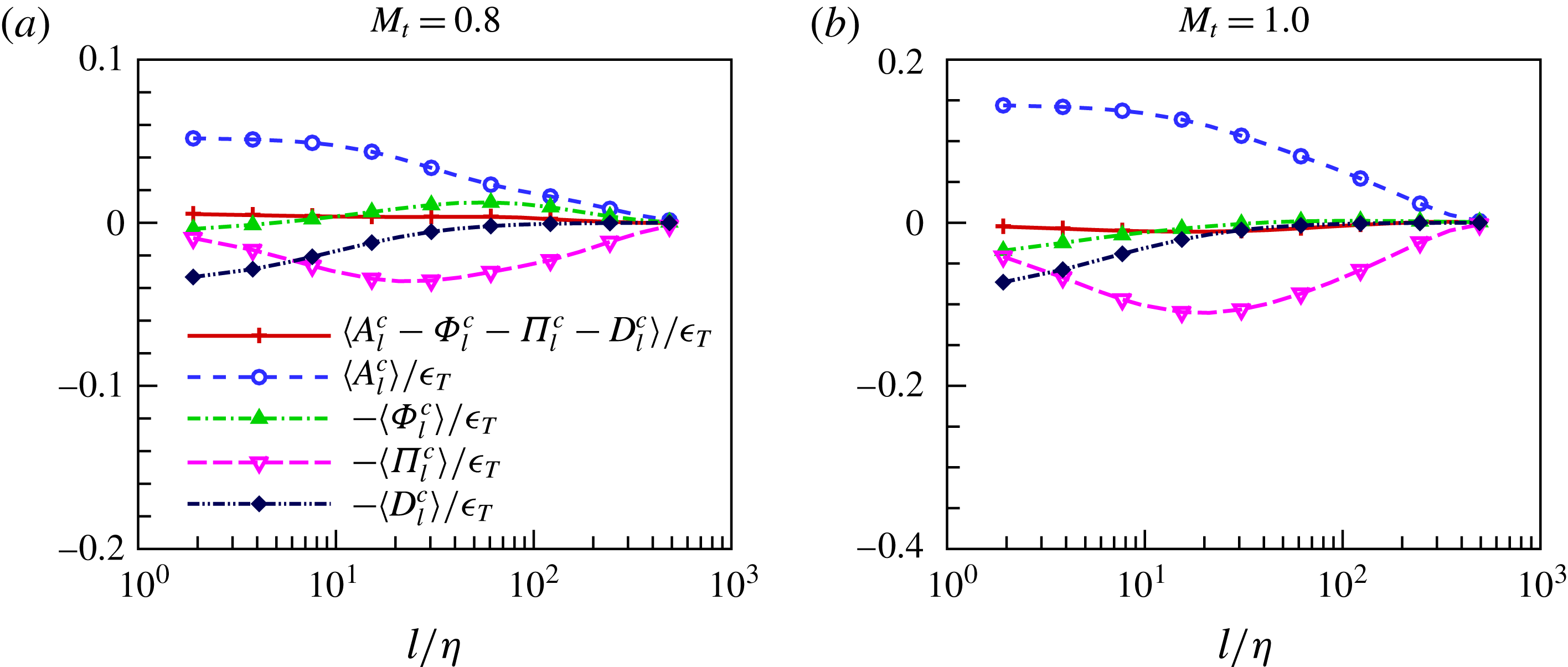
are non-negative, and increase rapidly with growing turbulent Mach number. Consequently, kinetic energy can be transferred from the solenoidal mode to the compressible mode by nonlinear advection. The increase of turbulent Mach number enhances the kinetic energy transfer between the two modes by nonlinear advection.
 $-\langle A_{l}^{s}\rangle /\unicode[STIX]{x1D716}_{T}$
and
 $\langle A_{l}^{c}\rangle /\unicode[STIX]{x1D716}_{T}$
also increase with the decrease of filter width. Therefore, we infer that during the cascade of solenoidal kinetic energy from large scales to small scales, the compressible mode will persistently absorb energy from the solenoidal mode through the nonlinear advection at different length scales. At
 $M_{t}=1.0$
, the overall energy transfer from the solenoidal mode to the compressible mode by nonlinear advection is close to
 $0.15$
.
Average of solenoidal and compressible components of the nonlinear advection: (a)
 $-\langle A_{l}^{s}\rangle /\unicode[STIX]{x1D716}_{T}$
and (b)
 $\langle A_{l}^{c}\rangle /\unicode[STIX]{x1D716}_{T}$
.

In figure 18, we plot average of energy transfer terms in the filtered equation of the compressible component of kinetic energy, at turbulent Mach numbers
 $M_{t}=0.8,1.0$
. The average pressure-dilatation term
 $-\langle \unicode[STIX]{x1D6F7}_{l}^{c}\rangle /\unicode[STIX]{x1D716}_{T}$
is always negligibly small. The average dissipation
 $-\langle D_{l}^{c}\rangle /\unicode[STIX]{x1D716}_{T}$
is negative and can substantially dissipate compressible kinetic energy at small scales
 $l/\unicode[STIX]{x1D702}\leqslant 10$
. As the filter width increases from
 $l/\unicode[STIX]{x1D702}=10$
, the magnitude of
 $-\langle D_{l}^{c}\rangle /\unicode[STIX]{x1D716}_{T}$
decays dramatically. The average nonlinear convection term
 $\langle A_{l}^{c}\rangle /\unicode[STIX]{x1D716}_{T}$
is always positive and can inject energy into the compressible mode at all scales. In contrast, the average SGS flux
 $-\langle \unicode[STIX]{x1D6F1}_{l}^{c}\rangle /\unicode[STIX]{x1D716}_{T}$
is always negative and can transfer compressible kinetic energy from large scale to small scales. At scales
 $l/\unicode[STIX]{x1D702}\geqslant 30$
, the nonlinear advection
 $\langle A_{l}^{c}\rangle /\unicode[STIX]{x1D716}_{T}$
is nearly balanced by the SGS flux
 $-\langle \unicode[STIX]{x1D6F1}_{l}^{c}\rangle /\unicode[STIX]{x1D716}_{T}$
, since both pressure term and dissipation term are very small.
Average of energy transfer terms in the filtered equation of compressible component of kinetic energy, at turbulent Mach numbers
 $M_{t}=0.8,1.0$
.

We show PDFs of the normalized compressible SGS flux
 $\unicode[STIX]{x1D6F1}_{l}^{c}/\unicode[STIX]{x1D716}_{T}$
at turbulent Mach numbers
 $M_{t}=0.4,0.6,0.8,1.0$
in figure 19. We observe that the tails of the PDF are longer at smaller filter width
 $l$
and at larger turbulent Mach number
 $M_{t}$
. At
 $M_{t}=0.4,0.6$
, the PDF is nearly symmetric, indicating that the positive part of compressible SGS flux is almost cancelled by the negative part, leading to the negligible net SGS flux of compressible kinetic energy. At
 $M_{t}=0.8,1.0$
, the PDF is skewed toward the positive side, suggesting that the direct SGS flux of compressible kinetic energy is larger than the reverse flux of compressible kinetic energy.
PDF of the normalized compressible SGS flux
 $\unicode[STIX]{x1D6F1}_{l}^{c}/\unicode[STIX]{x1D716}_{T}$
at turbulent Mach numbers
 $M_{t}=0.4,0.6,0.8,1.0$
.

Rescaled PDF of the normalized compressible SGS flux
 $l\unicode[STIX]{x1D6F1}_{l}^{c}/(\unicode[STIX]{x1D716}_{T}\unicode[STIX]{x1D702})$
at turbulent Mach numbers
 $M_{t}=0.8,1.0$
.

We depict the rescaled PDF of the normalized compressible SGS flux
 $l\unicode[STIX]{x1D6F1}_{l}^{c}/(\unicode[STIX]{x1D716}_{T}\unicode[STIX]{x1D702})$
at turbulent Mach numbers
 $M_{t}=0.8,1.0$
in figure 20. The right tails of the rescaled PDFs are likely to overlap one another for different filter width
 $l/\unicode[STIX]{x1D702}=16,24,32,48,64$
at
 $M_{t}=1.0$
. Similar to previous studies (Benzi et al.
Reference Benzi, Biferale, Fisher, Kadanoff, Lamb and Toschi2008; Yang et al.
Reference Yang, Wang, Shi, Xiao, He and Chen2016b
; Wang et al.
Reference Wang, Gotoh and Watanabe2017c
), the scaling exponents for the moments of
 $l\unicode[STIX]{x1D6F1}_{l}^{c}$
should saturate at the value of
 $z_{\infty }=1$
for high orders, i.e.
 $\langle |l\unicode[STIX]{x1D6F1}_{l}^{c}|^{n}\rangle \sim l^{z_{\infty }}$
for large
 $n$
, since the right tails of the PDFs have major contributions to the high-order moments of
 $l\unicode[STIX]{x1D6F1}_{l}^{c}$
. The saturated exponent
 $1.0$
suggests that the singularity structures of intensive values of
 $l\unicode[STIX]{x1D6F1}_{l}^{c}$
are sheet-like. The observation reveals a nearly statistical scale-invariant property of compressible energy flux
 $\unicode[STIX]{x1D6F1}_{l}^{c}$
in the range of
 $16\leqslant l/\unicode[STIX]{x1D702}\leqslant 64$
.
We provide isosurfaces of compressible SGS flux at
 $\unicode[STIX]{x1D6F1}_{l}^{c}/(\unicode[STIX]{x1D6F1}_{l}^{c})^{\prime }=2$
for the filter width
 $l/\unicode[STIX]{x1D702}=16$
, at turbulent Mach numbers
 $M_{t}=0.4,0.6,0.8,1.0$
in figure 21. The isosurfaces are coloured based on the normalized filtered velocity
 $\unicode[STIX]{x1D703}_{l}/\unicode[STIX]{x1D703}_{l}^{\prime }$
. Most isosurfaces are located in strong compression regions, suggesting that compression motions make a major contribution to the direct SGS flux of compressible kinetic energy. At
 $M_{t}=0.4$
, isosurfaces
 $\unicode[STIX]{x1D6F1}_{l}^{c}/(\unicode[STIX]{x1D6F1}_{l}^{c})^{\prime }=2$
are the mixture of sheet-like and blob-like structures, and are nearly uniformly distributed over the whole field. As turbulent Mach number increases from
 $0.4$
, the fraction of sheet-like structures in isosurfaces
 $\unicode[STIX]{x1D6F1}_{l}^{c}/(\unicode[STIX]{x1D6F1}_{l}^{c})^{\prime }=2$
increases gradually, demonstrating the significant effect of shocklets on the SGS flux of compressible kinetic energy. At
 $M_{t}=1.0$
, the length scales of sheet-like isosurfaces are relatively large, as compared to the situation of smaller turbulent Mach numbers.
Isosurfaces of compressible SGS flux at
 $\unicode[STIX]{x1D6F1}_{l}^{c}/(\unicode[STIX]{x1D6F1}_{l}^{c})^{\prime }=2$
for the filter width
 $l/\unicode[STIX]{x1D702}=16$
, at turbulent Mach numbers
 $M_{t}=0.4,0.6,0.8,1.0$
.

Isosurfaces of compressible SGS flux at
 $\unicode[STIX]{x1D6F1}_{l}^{c}/(\unicode[STIX]{x1D6F1}_{l}^{c})^{\prime }=-2$
for the filter width
 $l/\unicode[STIX]{x1D702}=16$
, at turbulent Mach numbers
 $M_{t}=0.4,0.6,0.8,1.0$
.

Isosurfaces of compressible SGS flux at
 $\unicode[STIX]{x1D6F1}_{l}^{c}/(\unicode[STIX]{x1D6F1}_{l}^{c})^{\prime }=-2$
is shown for the filter width
 $l/\unicode[STIX]{x1D702}=16$
, at turbulent Mach numbers
 $M_{t}=0.4,0.6,0.8,1.0$
in figure 22. The isosurfaces are coloured based on the normalized filtered velocity
 $\unicode[STIX]{x1D703}_{l}/\unicode[STIX]{x1D703}_{l}^{\prime }$
. Most isosurfaces are located in strong expansion regions, suggesting that expansion motions make a major contribution to the reverse SGS flux of compressible kinetic energy. The isosurfaces are the mixture of sheet-like and blob-like structures. At
 $M_{t}=0.4$
, isosurfaces
 $\unicode[STIX]{x1D6F1}_{l}^{c}/(\unicode[STIX]{x1D6F1}_{l}^{c})^{\prime }=-2$
are nearly uniformly distributed over the whole field, which are quite similar to isosurfaces
 $\unicode[STIX]{x1D6F1}_{l}^{c}/(\unicode[STIX]{x1D6F1}_{l}^{c})^{\prime }=2$
. At
 $M_{t}=1.0$
, the spatial patterns of the isosurfaces
 $\unicode[STIX]{x1D6F1}_{l}^{c}/(\unicode[STIX]{x1D6F1}_{l}^{c})^{\prime }=-2$
exhibit substantial intermittency. The structures of isosurfaces
 $\unicode[STIX]{x1D6F1}_{l}^{c}/(\unicode[STIX]{x1D6F1}_{l}^{c})^{\prime }=-2$
and
 $\unicode[STIX]{x1D6F1}_{l}^{c}/(\unicode[STIX]{x1D6F1}_{l}^{c})^{\prime }=2$
are very different at
 $M_{t}=1.0$
: isosurfaces
 $\unicode[STIX]{x1D6F1}_{l}^{c}/(\unicode[STIX]{x1D6F1}_{l}^{c})^{\prime }=-2$
are blob-like, associated with strong expansion, while isosurfaces
 $\unicode[STIX]{x1D6F1}_{l}^{c}/(\unicode[STIX]{x1D6F1}_{l}^{c})^{\prime }=2$
are sheet-like, associated with strong compression, demonstrating the distinct effects of expansion motions and compression motions on the SGS flux of compressible kinetic energy.
Average of normalized compressible SGS flux
 $\unicode[STIX]{x1D6F1}_{l}^{c}/\unicode[STIX]{x1D716}_{T}$
conditioned on the normalized filtered velocity divergence
 $\unicode[STIX]{x1D703}_{l}/\unicode[STIX]{x1D703}_{l}^{\prime }$
for different filter widths
 $l/\unicode[STIX]{x1D702}=16,24,32,48,64$
at turbulent Mach numbers
 $M_{t}=0.4,0.6,0.8,1.0$
.

We display the average of normalized compressible SGS flux
 $\unicode[STIX]{x1D6F1}_{l}^{c}/\unicode[STIX]{x1D716}_{T}$
conditioned on the normalized filtered velocity divergence
 $\unicode[STIX]{x1D703}_{l}/\unicode[STIX]{x1D703}_{l}^{\prime }$
for different filter widths
 $l/\unicode[STIX]{x1D702}=16,24,32,48,64$
at turbulent Mach numbers
 $M_{t}=0.4,0.6,0.8,1.0$
in figure 23. The conditional average of compressible SGS flux is nearly independent of filter width
 $l/\unicode[STIX]{x1D702}$
, for
 $16\leqslant l/\unicode[STIX]{x1D702}\leqslant 64$
at moderate and high turbulent Mach numbers
 $0.6\leqslant M_{t}\leqslant 1.0$
. Moreover, the conditional average
 $\langle \unicode[STIX]{x1D6F1}_{l}^{c}/\unicode[STIX]{x1D716}_{T}|\unicode[STIX]{x1D703}_{l}/\unicode[STIX]{x1D703}_{l}^{\prime }\rangle$
is positive in the compression region and is negative in the expansion region. Thus, compression motions cause the direct SGS flux of compressible kinetic energy, while expansion motions cause the reverse SGS flux of compressible kinetic energy. A simple model for the conditional average of compressible SGS flux in compression regions
 $\unicode[STIX]{x1D703}_{l}\leqslant 0$
is proposed as:
 $$\begin{eqnarray}\displaystyle & \displaystyle \left\langle \unicode[STIX]{x1D6F1}_{l}^{c}/\unicode[STIX]{x1D716}_{T}\big|\unicode[STIX]{x1D703}_{l}/\unicode[STIX]{x1D703}_{l}^{\prime }\right\rangle =\unicode[STIX]{x1D6FC}_{0}^{c}M_{t}^{3}\left(\unicode[STIX]{x1D703}_{l}/\unicode[STIX]{x1D703}_{l}^{\prime }\right)^{2}, & \displaystyle\end{eqnarray}$$
where,
 $\unicode[STIX]{x1D6FC}_{0}^{c}=0.23$
. The equation (5.4) is consistent with the numerical results at
 $M_{t}=0.8,1.0$
. It is straightforward to derive the following relation in compression regions
 $\unicode[STIX]{x1D703}_{l}\leqslant 0$
:
 $$\begin{eqnarray}\displaystyle & \displaystyle \left\langle \unicode[STIX]{x1D6F1}_{l}^{s}/\unicode[STIX]{x1D716}_{T}\big|\unicode[STIX]{x1D703}_{l}/\unicode[STIX]{x1D703}_{l}^{\prime }\right\rangle =1+\unicode[STIX]{x1D6FC}_{0}^{s}M_{t}^{3}\left(\unicode[STIX]{x1D703}_{l}/\unicode[STIX]{x1D703}_{l}^{\prime }\right)^{2}, & \displaystyle\end{eqnarray}$$
where,
 $\unicode[STIX]{x1D6FC}_{0}^{s}=\unicode[STIX]{x1D6FC}_{0}-\unicode[STIX]{x1D6FC}_{0}^{c}=0.19$
. It is worth noting that
 $\unicode[STIX]{x1D6FC}_{0}^{c}>\unicode[STIX]{x1D6FC}_{0}^{s}$
, which indicates that the local SGS kinetic energy transfer of compressible mode is affected by strong compression motions more significantly, as compared to its solenoidal counterpart.
Average of normalized compressible SGS flux
 $\unicode[STIX]{x1D6F1}_{l}^{c}/\unicode[STIX]{x1D716}_{T}$
conditioned on the normalized filtered velocity divergence
 $\unicode[STIX]{x1D703}_{l}/\unicode[STIX]{x1D703}_{l}^{\prime }$
for different filter widths
 $l/\unicode[STIX]{x1D702}=16,24,32,48,64$
in expansion regions. Here,
 $\unicode[STIX]{x1D6FC}_{1}^{c}=0.15,0.27,0.36,0.45$
for turbulent Mach numbers
 $M_{t}=0.4,0.6,0.8,1.0$
, respectively.

In figure 24, we plot the conditional average of normalized compressible SGS flux
 $\unicode[STIX]{x1D6F1}_{l}^{c}/\unicode[STIX]{x1D716}_{T}$
for different filter widths
 $l/\unicode[STIX]{x1D702}=16,24,32,48,64$
in expansion regions
 $\unicode[STIX]{x1D703}_{l}\geqslant 0$
. We propose a simple model for the conditional average of compressible SGS flux in expansion regions
 $\unicode[STIX]{x1D703}_{l}\geqslant 0$
:
 $$\begin{eqnarray}\displaystyle & \displaystyle \left\langle \unicode[STIX]{x1D6F1}_{l}^{c}/\unicode[STIX]{x1D716}_{T}\big|\unicode[STIX]{x1D703}_{l}/\unicode[STIX]{x1D703}_{l}^{\prime }\right\rangle =-\unicode[STIX]{x1D6FC}_{1}^{c}\left(\unicode[STIX]{x1D703}_{l}/\unicode[STIX]{x1D703}_{l}^{\prime }\right)^{1.2}, & \displaystyle\end{eqnarray}$$
where,
 $\unicode[STIX]{x1D6FC}_{1}^{c}=0.15,0.27,0.36,0.45$
for turbulent Mach numbers
 $M_{t}=0.4,0.6,0.8,1.0$
, respectively. The equation (5.6) is consistent with the numerical results at
 $M_{t}=0.6,0.8,1.0$
. It is straightforward to derive the following model in the expansion regions
 $\unicode[STIX]{x1D703}_{l}\geqslant 0$
:
 $$\begin{eqnarray}\displaystyle & \displaystyle \left\langle \unicode[STIX]{x1D6F1}_{l}^{s}/\unicode[STIX]{x1D716}_{T}\big|\unicode[STIX]{x1D703}_{l}/\unicode[STIX]{x1D703}_{l}^{\prime }\right\rangle =1-\unicode[STIX]{x1D6FC}_{1}^{s}\left(\unicode[STIX]{x1D703}_{l}/\unicode[STIX]{x1D703}_{l}^{\prime }\right)^{1.2}, & \displaystyle\end{eqnarray}$$
where,
 $\unicode[STIX]{x1D6FC}_{1}^{s}=\unicode[STIX]{x1D6FC}_{1}-\unicode[STIX]{x1D6FC}_{1}^{c}=0.10,0.28,0.44,0.55$
for turbulent Mach numbers
 $M_{t}=0.4,0.6,0.8,1.0$
, respectively. We show that
 $\unicode[STIX]{x1D6FC}_{1}^{s}>\unicode[STIX]{x1D6FC}_{1}^{c}$
at
 $M_{t}=0.6,0.8,1.0$
.
6 Summary and conclusions
In this paper, a filtering method is applied to investigate inter-scale kinetic energy transfer in solenoidally forced stationary compressible isotropic turbulence at turbulent Mach numbers from
 $0.4$
to
 $1.0$
. The average pressure dilatation is negligibly small. The average viscous dissipation is important at small scales
 $l/\unicode[STIX]{x1D702}\leqslant 10$
, and decreases rapidly as the filter width increases from
 $10$
, which is consistent with the previous theoretical analysis of the viscous dissipation in compressible flows. In the range of
 $30\leqslant l/\unicode[STIX]{x1D702}\leqslant 200$
, the average SGS flux makes a major contribution to the net transfer of filtered kinetic energy. The normalized r.m.s. value of SGS flux increases with the increase of turbulent Mach number, demonstrating the significant compressibility effect on the local transfer of kinetic energy by SGS stress. The normalized r.m.s. value of pressure dilatation is larger than 1.0, implying that the local conversion between kinetic energy and internal energy by pressure work is significant. The negligible contribution of pressure dilatation to the net transfer of kinetic energy is due to the cancellation between compression and expansion works.
The compressibility effect on the SGS flux of kinetic energy is further investigated. The right tail of the PDF of the SGS flux becomes longer as the turbulent Mach number increases. After decomposing the SGS flux into a positive component and a negative component, it is found that the ratio of average negative SGS flux to the average SGS flux increases with the increase of turbulent Mach number. Thus, the backscatter of kinetic energy is more significant at higher turbulent Mach numbers. As turbulent Mach number increases, the positive SGS flux is suppressed in expansion regions and is enhanced in compression regions. In contrast, the negative SGS flux is enhanced in expansion regions, and is negligibly small in compression regions. The shape of the joint PDF of the SGS flux and the filtered velocity divergence is nearly symmetric at
 $M_{t}=0.4$
, and tends to concentrate in the second and fourth quadrants as
 $M_{t}$
increases from
 $0.4$
. At
 $0.6\leqslant M_{t}\leqslant 1.0$
, compression motions make a major contribution to the positive SGS flux of kinetic energy, while expansion motions make a major contribution to the negative SGS flux of kinetic energy. As turbulent Mach number increases, the isosurfaces of positive SGS flux tend to be sheet-like, which are different from the blob-like structures of the isosurfaces of negative SGS flux.
The average of SGS flux conditioned on the filtered velocity divergence is investigated. The conditional average of SGS flux is nearly independent of filter width in the range of
 $16\leqslant l/\unicode[STIX]{x1D702}\leqslant 64$
, at moderate and high turbulent Mach numbers
 $0.6\leqslant M_{t}\leqslant 1.0$
. A simple heuristic model is constructed for the relation between the conditional average of SGS flux and the filtered velocity divergence, which is found to be consistent with the numerical simulations. Particularly, the conditional average of SGS flux is proportional to the square of filtered velocity divergence in strong compression regions. In addition, the antiparallel alignment between the large-scale strain and the SGS stress is identified in strong compression regions. The study of conditional average shows again that strong compression motions induce the direct SGS flux of kinetic energy from large scales to small scales, and strong expansion motions induce the reverse SGS flux of kinetic energy from small scales to large scales.
Helmholtz decomposition is employed to study the inter-scale energy transfer of the solenoidal mode and compressible mode. It is shown that the SGS flux of the solenoidal kinetic energy is almost independent of the turbulent Mach number, while the SGS flux of the compressible kinetic energy is enlarged drastically by the increase of the turbulent Mach number. It is further revealed that nonlinear advection transfers the kinetic energy from the solenoidal mode to the compressible mode. The SGS stress transfers the kinetic energy of compressible mode from large scales to small scales. At small scales
 $l/\unicode[STIX]{x1D702}\leqslant 10$
, the viscosity irreversibly dissipates the compressible kinetic energy into internal energy.
The PDF of the normalized compressible SGS flux is nearly symmetric at
 $M_{t}=0.4,0.6$
, and is skewed toward the positive side at
 $M_{t}=0.8,1.0$
. The tails of the PDF becomes longer as the turbulent Mach number increases. After proper normalization, the right tails of rescaled PDFs of the normalized compressible SGS flux
 $l\unicode[STIX]{x1D6F1}_{l}^{c}/(\unicode[STIX]{x1D716}_{T}\unicode[STIX]{x1D702})$
overlap one another for different filter widths
 $l/\unicode[STIX]{x1D702}=16,24,32,48,64$
at
 $M_{t}=1.0$
, revealing the statistical scale-invariant property of compressible kinetic energy flux. Isosurfaces of positive compressible SGS flux are strongly correlated with compression motions, while isosurfaces of negative compressible SGS flux are strongly correlated with expansion motions. The conditional average of compressible SGS flux is proportional to the square of filtered velocity divergence in compression regions.
In conclusion, a variety of effects of compression motions and expansion motions on the SGS flux of the kinetic energy are revealed through numerical simulations of stationary compressible isotropic turbulence driven by purely solenoidal forcing. The statistics and structures of SGS flux of kinetic energy exhibit distinct features at a high turbulent Mach number of
 $1.0$
, as compared to those at a low turbulent Mach number of
 $0.4$
. When developing SGS models for LES of highly compressible turbulence, these new features need to be taken into account to ensure accurate prediction by LES.
Acknowledgements
The authors appreciate the valuable comments of the anonymous referees. This work was supported by the National Natural Science Foundation of China (NSFC grants no. 11702127, no. 91752201 and no. 11672123), by ‘the Thousand Young Talents Plan for Young Professionals’, and by the Technology and Innovation Commission of Shenzhen Municipality (grant no. JCYJ20170412151759222). J.W. acknowledges the support from Young Elite Scientist Sponsorship Program by CAST (grant no. 2016QNRC001).