1 Introduction
In ocean engineering, coastal engineering and naval architecture applications, extreme wave impact can cause serious damage to structures and ships, due to the tremendous momentum carried by high-speed water jets that are generated during the impact process or due to the very high subsurface transient pressures that are created. Since the present work addresses the impact of a two-dimensional (2-D) breaking wave on the vertical front surface of a 2-D structure, the following literature review is confined to studies with similarly restricted wave and structural geometries. This restricted type of impact problem is both practically important and well suited to the exploration of the physics of impact phenomena.
The impact process starts with the behaviour of the wave, in this case, a plunging breaker. Plunging breaking waves are commonly seen in both shallow water and deep water. In the process of breaking, as the crest steepens, a jet issues from the crest and grows horizontally in the direction of propagation. The jet subsequently falls due to gravity and impacts the water surface upstream of the crest. During this transient nonlinear process, turbulence, splashes, droplets and air bubbles are generated. Plunging breaking waves have been studied by many investigators both experimentally (see for example Rapp & Melville Reference Rapp and Melville1990; Perlin, He & Bernal Reference Perlin, He and Bernal1996) and computationally (see for example Longuet-Higgins & Cokelet Reference Longuet-Higgins and Cokelet1976; Dommermuth et al. Reference Dommermuth, Yue, Lin, Rapp, Chan and Melville1988).
The impact of a two-dimensional plunging breaker on a wall with relatively large vertical extent compared to the wavelength has received considerable attention in the literature. The wave impact behaviour can be divided into several regimes based on the streamwise position of the wall relative to the location where the wave breaks in the absence of the wall (defined herein as open water). Following this idea, Chan & Melville (Reference Chan and Melville1988) performed an experimental study of the deep-water breaking wave impact on a 2-D wall that extended to the bottom of the tank. If the wall is positioned some distance downstream of the open-water wave breaking location, the post-breaking turbulent crest of the wave interacts with the wall. According to Chan & Melville (Reference Chan and Melville1988), double pressure peaks are possible in this range of wall locations in cases where a secondary jet that originates from the impact of the main plunging jet into the water collides with the wall before the turbulent breaking region of the wave. If the wall is located at a position far upstream of the open-water breaking location, the breaker is not fully developed before reaching the wall and the impact phenomenon is relatively weak without violent impact pressure.
At a critical wall position between the above two cases, a jet begins to form as the crest reaches the wall and at the same time the contact point of the water surface on the wall is moving upwards and meets the crest. In this case, the impact does not involve breaking as the water surface profile undergoes a phenomenon called ‘flip through’, see Peregrine (Reference Peregrine2003), in which a high-speed vertical jet is formed and very high wall pressures are developed, as described below. In this process, the fluid domain stays as a simply connected region without entraining air bubbles. Flip-through-like phenomena also occur in some other free surface flow problems that involve the formation of a high-speed jet, including standing waves (Zeff et al. Reference Zeff, Kleber, Fineberg and Lathrop2000; Longuet-Higgins Reference Longuet-Higgins2001), capillary pinch off of droplets (Day, Hinch & Lister Reference Day, Hinch and Lister1998; Leppinen & Lister Reference Leppinen and Lister2003), collapsing bubbles near a solid boundary (Zhang, Duncan & Chahine Reference Zhang, Duncan and Chahine1993; Longuet-Higgins & Oguz Reference Longuet-Higgins and Oguz1995) and sloshing (Lugni, Brocchini & Faltinsen Reference Lugni, Brocchini and Faltinsen2006).
By using a potential flow formulation, flip-through phenomena have been investigated in several theoretical studies. Longuet-Higgins & Oguz (Reference Longuet-Higgins and Oguz1997) used a single term solution to Laplace’s equation with power-law temporal dependence of the velocity potential to model the unsteady flow field. In this model, the surface in the far-field asymptotically approaches a constant slope, which is related to the order of the single term solution as well as the decay rate of the length scale. However, the single term analytic solution can only qualitatively describe a free surface with the far-field slope close to
 $\unicode[STIX]{x03C0}/2$
. Longuet-Higgins (Reference Longuet-Higgins2001) used model equations to study the high-speed vertical jet produced by 2-D standing waves under critical conditions. By properly choosing the initial shape of the standing wave, the acceleration of the free surface is found to reach over
 $10g$
, where
 $g=9.81~\text{m}~\text{s}^{-2}$
is the gravitational acceleration. In this work, Longuet-Higgins also studied the effect of initial profile perturbations on the acceleration of the jet. It is pointed out that the maximum acceleration is sensitive to the initial shape of the surface and the small perturbations can further increase the maximum acceleration.
Extreme wall pressures during various wave impact types have been reported by many investigators, both in laboratory and field experiments. Bagnold (Reference Bagnold1939) conducted an experimental study of the wall pressure generated during shallow-water wave impact on a wall and developed a theoretical model to estimate the impact pressure. The wave was steepened to break by a sloped beach at the bottom of the tank. It was concluded that extreme pressures are generated by the direct impact of a nearly vertical water surface on the wall along with a variable thickness air cushion between the wall and the wave front. The maximum pressure occurs when the thickness of the cushion is a minimum. Blackmore & Hewson (Reference Blackmore and Hewson1984) made full-scale field measurements of impact pressure on a sea wall while Kirkgöz (Reference Kirkgöz1991) and Bullock et al. (Reference Bullock, Obhrai, Peregrine and Bredmose2007) measured wave impact pressure on vertical and sloping walls (reaching the tank bottom). Lugni et al. (Reference Lugni, Miozzi, Brocchini and Faltinsen2010b ) and Lugni, Brocchini & Faltinsen (Reference Lugni, Brocchini and Faltinsen2010a ) measured wall pressures in a study of the impact of waves on the vertical wall of a rectangular tank partially filled with water and undergoing a horizontal sinusoidal motion. Bagnold (Reference Bagnold1939) and Chan & Melville (Reference Chan and Melville1988) both reported the run-to-run variability of the impact pressure even under very consistent experimental conditions.
Several investigations of wall pressure during wave impact have focused on flip-through conditions, which, as mentioned above, occur without direct impact of the water surface on the wall. This mechanism was first reported in the numerical simulation of a flip-through shallow-water wave impact on a wall by Cooker & Peregrine (Reference Cooker, Peregrine, Banner and Grimshaw1992). The mechanism by which these high pressures are created was explored by Cooker (Reference Cooker2002). In this study, analytic models are introduced to describe several types of focusing flow with simplified boundary geometries. The models employ basic potential flow singularities to represent the flow field at one instant in time and the theory allows for the computation of the associated pressure field. It is found that in the absence of gravity, there exists a pressure peak just below the surface. Bredmose, Peregrine & Bullock (Reference Bredmose, Peregrine and Bullock2009) also showed this mechanism of extreme pressure generation in a simulation of flip through in a shallow-water wave impact problem. For wave impact in a sloshing experiment in a rectangular box, such a mechanism has been reported by Lugni et al. (Reference Lugni, Brocchini and Faltinsen2006). These high pressures appear just below the free surface, indicating that high subsurface pressure gradient and flow acceleration exist. In the Cooker & Peregrine (Reference Cooker, Peregrine, Banner and Grimshaw1992) simulations, flow accelerations of more than
 $1000g$
were found just as the vertical jet forms. Similar flow accelerations (
 $1,500g$
) have been found in the sloshing experiments of Lugni et al. (Reference Lugni, Brocchini and Faltinsen2006).
In addition to the air entrainment that occurs when the wave breaks before impact with the wall as described in Chan & Melville (Reference Chan and Melville1988) and mentioned above, air entrainment can occur when the plunging jet directly hits the wall and encloses a pocket of air. The influence of the entrained air on the flow, and the impact pressure when an air pocket is enclosed has been studied extensively in experiments and theory. Bagnold (Reference Bagnold1939) mentioned the cushion effect of the air phase can decrease the impact pressure. It is also mentioned that the thickness of the air cushion is important and that the thickness is not uniform along the impact zone due to the irregularity of the wave crest. This effect is thought to contribute to the variation of pressure along the impact zone. Peregrine & Thais (Reference Peregrine and Thais1996) developed a method for estimating the effect of an air cushion on the wave impact pressure. In their work, the aerated water is assumed to be a mixture of an incompressible liquid and a distribution of small air-filled, i.e. compressible, spherical bubbles. Their results show that the Mach number of the incoming flow and the severity of the wave can affect the pressure reduction due to the air cushion during impact. Their method also suggests that even a small fraction of air dispersed as small bubbles in the flow can decrease the impact pressure significantly. Bredmose et al. (Reference Bredmose, Peregrine and Bullock2009) studied the effect of air during wave impact by numerical simulations. Similar to Bagnold (Reference Bagnold1939), they found the pressure is maximum when only a small pocket of air is trapped. The trapped air tends to decrease the maximum pressure and increase the impulse and force because the increase in the area and duration of the impact.
The presence of entrained air makes it difficult to predict full-scale wave impact phenomenon based on prototype-scale experiments. Traditional Froude scaling can overestimate the impact pressure in cases with air entrainment (see Bullock et al.
Reference Bullock, Crawford, Hewson, Walkden and Bird2001), because the cushion effect of the air phase is not taken into account. Zhang, Yue & Tanizawa (Reference Zhang, Yue and Tanizawa1996) pointed out that when
 $P_{0}/\unicode[STIX]{x1D70C}U^{2}\ll 1$
, where
 $P_{0}$
is the initial pressure of the air pocket,
 $U$
is the plunging jet tip velocity and
 $\unicode[STIX]{x1D70C}$
is the density of water, the scaling factor of maximum pressure
 $P_{m}/\unicode[STIX]{x1D70C}U^{2}$
is only a function of the geometry of the plunging jet. If
 $P_{0}/\unicode[STIX]{x1D70C}U^{2}\sim O(1)$
, the scaling factor is a function of the geometry of both the plunging jet and the air pocket. In the latter case, the oscillations of the air pocket are modelled as a spring–mass system. Bredmose, Bullock & Hogg (Reference Bredmose, Bullock and Hogg2015) also discussed scaling of the impact pressure in the presence of entrained air. In this work, it is suggested that Froude scaling works for flip-through impact and in circumstances with air entrainment when the impact pressure is low. Air entrainment with high impact pressure follows Bagnold–Mitsuyasu scaling, as discussed by Bredmose et al. (Reference Bredmose, Bullock and Hogg2015).
Wave impact with structures such that the distance between the bottom of a structure and the mean water level is small compared with both the wavelength and the water depth have not been studied in detail before. This type of impact is more complex than the cases discussed so far. Obvious configurations where this set-up will produce new impact phenomena are when the bottom of the structure is located near the mean water level and when the bottom of the structure is located just below the height of the wave crest. In the former case, the bottom of the structure transitions back and forth between above and below the local water level during the impact process, while in the latter case, the structure is only hit by the wave crest as the wave propagates as if in open water up until the instant before impact. Examples of practical applications which feature this type of impact include moored drill ships being hit broadside by waves, simulated in the experiments when the bottom of the structure is below the mean water level, and drilling platforms on various types of support legs, simulated in the experiments when the bottom of the structure is above the mean water level.
In this paper, an experimental investigation of the impact of a deep-water wave on a 2-D structure with its bottom located near the mean water level is presented. Specifically, we study wave impact for one wave maker motion and nine vertical positions of the structure when it is located horizontally at one distance from the wave maker. The following presentation of this work is divided into four sections. The experimental details are described in § 2 and the experimental results are presented in § 3. The detailed features of the water surface evolution and impact pressure are discussed in § 4. Finally, the conclusions are drawn in § 5.
2 Experimental details
2.1 Facilities
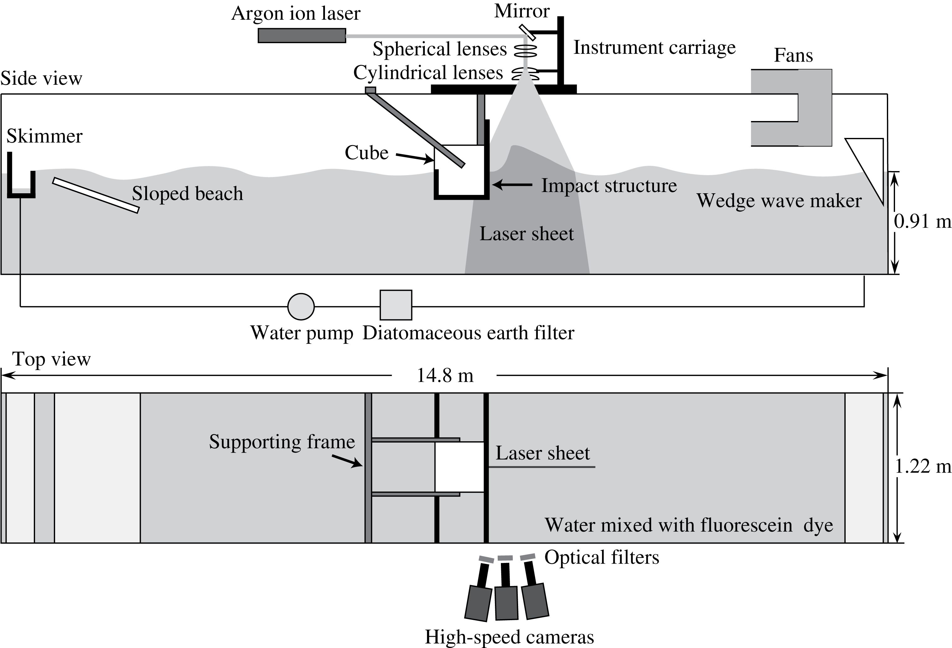
The experiments were performed in a wave tank that is 14.8 m long, 1.2 m wide and 2.2 m tall, see figure 1. The inside surface of the tank consists of a set of large flat panels which are in turn supported by an external superstructure consisting of steel beams. All of the floor panels and the wall panels at the two ends of the tank are made of 0.635 cm-thick stainless steel plates, while the panels on the long side walls of the tank are made of 3.5 cm-thick clear acrylic. The undisturbed water depth was 0.91 m for all experiments described herein.
Schematic of the wave tank.

The tank includes a programmable wave maker consisting of a vertically oscillating wedge that spans the width of the tank at one end. The side of the wedge closest to the end wall of the tank is vertical and the opposite side of the wedge is inclined at an angle of
 $30^{\circ }$
from vertical. The wedge is driven by a ball-screw and linear-bearing mechanism that is in turn driven by a servo-motor. A computer-based feedback control system is used with a position sensor and a motor tachometer to provide precise control of the motion of the wedge. Repeated tests with the same wave maker input parameters indicate only a
 $\pm 0.1\,\%$
root-mean-square error in wedge position at the time of peak displacement from the mean water level. In all experiments described herein, the wedge was oscillated about a mean level with the vertex of the wedge submerged 44.3 cm below the mean water level.
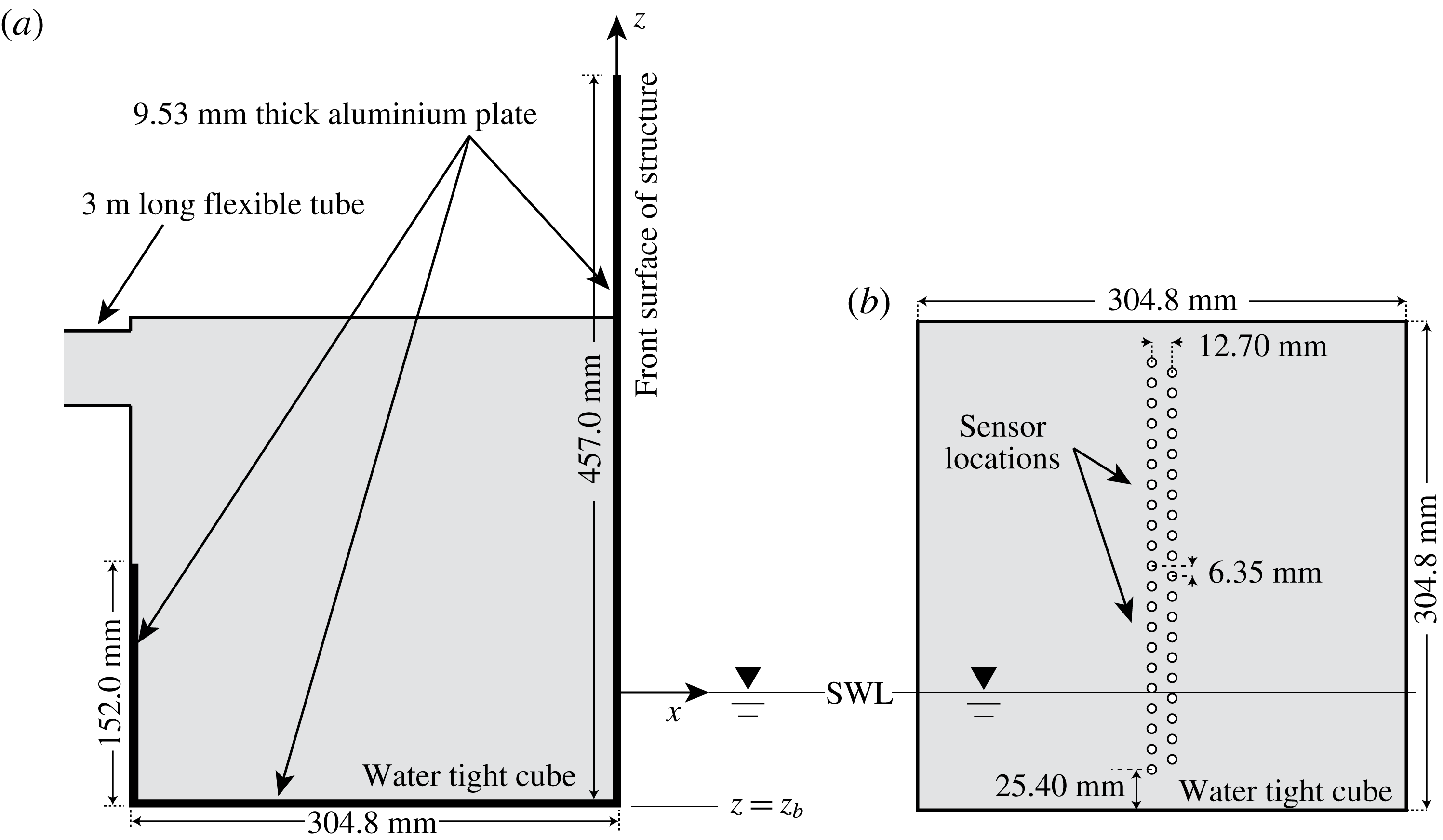
The wave impact occurs on a structure that interacts with the flow through three plane surfaces that span the width of the tank: a vertical forward face (45.7 cm tall), a vertical back face (15.2 cm tall) and a horizontal bottom face (30.4 cm wide), see figures 1 and 2(a). The bottom centrepiece of the structure is a sealed 30.48 cm cube whose front, bottom and back faces are coplanar with the corresponding faces of the structure. The front face of the cube has mounting holes for pressure sensors as shown in figure 2(b) and described in § 2.4. The entire structure is rigidly mounted to the top of the wave tank and can be moved to a wide range of vertical and streamwise horizontal positions within the tank.
Side view (a) of the impact structure and close up view (b) of the front face of the water-tight cube in which the pressure sensors are mounted. The cube walls are made of aluminium and the front face is 19.1 mm thick. The other 5 walls of the cube are 12.7 mm thick. The tube that comes out of the back face of the cube, see side view (a), is used to guide the electrical cables from the 24 pressure sensors to the A/D conversion system that is located outside of the tank. The purpose of the cube and the flexible tube is to keep the back face of the sensors and the cables dry. SWL is the still (undisturbed) water level.

A fixed skimmer is located at the opposite end of the tank from the wave maker and a removable skimmer is placed just upstream of the structure during the time between experimental runs. Water from the skimmers is pumped through a diatomaceous earth filter and then back into the tank at the upstream end, i.e. near the wave maker. Two fans are used at low speed between experimental runs to blow the water surface layer toward the skimmers, see below for detailed procedures.
2.2 Breaking wave generation
The breaking wave is generated by using a dispersively focused wave packet technique that was developed by Longuet-Higgins (Reference Longuet-Higgins, Cooper and Doroff1974) and used extensively by Rapp & Melville (Reference Rapp and Melville1990), Duncan et al. (Reference Duncan, Qiao, Philomin and Wenz1999) and others. In the present implementation of this technique, the wave maker motion is given by
 $$\begin{eqnarray}\displaystyle & \displaystyle z_{w}=w(t)\frac{2\unicode[STIX]{x03C0}}{N}A\mathop{\sum }_{i=1}^{N}\frac{1}{k_{0}}\left(\frac{k_{0}}{k_{i}}\right)^{q}\cos \left[x_{b}\left(\frac{\unicode[STIX]{x1D714}_{i}}{\bar{c}_{g}}-k_{i}\right)-\unicode[STIX]{x1D714}_{i}t+\unicode[STIX]{x1D719}\right], & \displaystyle\end{eqnarray}$$
where
 $w(t)$
is a window function described below,
 $N$
is the number of wave components,
 $A$
is a dimensionless constant representing the overall amplitude, (
 $k_{i}$
,
 $\unicode[STIX]{x1D714}_{i}$
) are the wavenumber and frequency of the
 $i\text{th}$
wave component (by linear theory,
 $k_{i}=\unicode[STIX]{x1D714}_{i}^{2}/g$
),
 $k_{0}=\overline{\unicode[STIX]{x1D714}}^{2}/g$
(where
 $\overline{\unicode[STIX]{x1D714}}$
is the average of the
 $N$
frequencies),
 $\bar{c}_{g}=(1/N)\sum _{i=1}^{N}0.5\unicode[STIX]{x1D714}_{i}/k_{i}$
is the average group velocity,
 $x_{b}$
is the streamwise position of the location of maximum amplitude based on linear theory and
 $q$
is an exponent chosen to distribute the wave amplitude among the various components. The frequencies are equally spaced,
 $\unicode[STIX]{x1D714}_{i}=\bar{\unicode[STIX]{x1D714}}-\unicode[STIX]{x0394}\unicode[STIX]{x1D714}/2+(i-1)\unicode[STIX]{x0394}\unicode[STIX]{x1D714}/(N-1)$
. The window function
 $w(t)$
is introduced in order to give the wave maker nearly zero motion at times when the summation of all the components generates a very small motion:
 $$\begin{eqnarray}\displaystyle & \displaystyle w(t)=0.25(1+\tanh (\unicode[STIX]{x1D6FD}f_{0}(t-t_{1})))(1-\tanh (\unicode[STIX]{x1D6FD}f_{0}(t-t_{2}))). & \displaystyle\end{eqnarray}$$
The value of the window function is zero when
 $t<t_{1}$
or
 $t>t_{2}$
and close to 1 when
 $t_{1}<t<t_{2}$
.
 $t_{1}$
and
 $t_{2}$
are given by
 $$\begin{eqnarray}\displaystyle & \displaystyle t_{1}f_{0}=\frac{x_{b}}{2\unicode[STIX]{x03C0}}\left(\frac{\bar{\unicode[STIX]{x1D714}}}{\bar{c_{g}}}-\frac{\bar{\unicode[STIX]{x1D714}}}{c_{N}}\right) & \displaystyle\end{eqnarray}$$
 $$\begin{eqnarray}\displaystyle & \displaystyle t_{2}f_{0}=\frac{x_{b}}{2\unicode[STIX]{x03C0}}\left(\frac{\bar{\unicode[STIX]{x1D714}}}{\bar{c_{g}}}-\frac{\bar{\unicode[STIX]{x1D714}}}{c_{1}}\right)+D\frac{x_{b}}{2\unicode[STIX]{x03C0}}\frac{\bar{\unicode[STIX]{x1D714}}}{\bar{c_{g}}} & \displaystyle\end{eqnarray}$$
so that the wave maker motion can allow the fastest component (with smallest frequency) and the slowest component (with largest frequency) to travel to the desired breaking location.
 $\unicode[STIX]{x1D6FD}$
is a constant that determines the rise rate of the window function, chosen as 5.0.
 $D$
is a dimensionless parameter, chosen as 0.507.
All of the experiments described herein were performed with the following set of wave maker motion parameters:
 $N=32$
,
 $A=0.0688$
,
 $\unicode[STIX]{x0394}\unicode[STIX]{x1D714}=0.77\bar{\unicode[STIX]{x1D714}}$
,
 $\bar{\unicode[STIX]{x1D714}}=7.226~\text{s}^{-1}$
and
 $x_{b}=7.15\unicode[STIX]{x1D706}_{0}$
, where
 $\unicode[STIX]{x1D706}_{0}=2\unicode[STIX]{x03C0}g/\bar{\unicode[STIX]{x1D714}}^{2}=1.181~\text{m}$
. These parameters yield
 $f_{0}=\bar{\unicode[STIX]{x1D714}}/(2\unicode[STIX]{x03C0})=1.15~\text{Hz}$
,
 $\overline{c}_{g}=0.7138~\text{m}~\text{s}^{-1}$
and characteristic wave phase speed
 $\bar{c_{p}}=2\bar{c_{g}}=1.437~\text{m}~\text{s}^{-1}$
. It should be noted that
 $x_{b}=8.441~\text{m}$
while the streamwise position of the front surface of the structure is 6.415 m from the vertical surface of the wedge. A record of surface elevation versus time at a position 250.2 cm upstream (toward the wave maker) from the position of the front face of the impact structure, which was not in the tank when this measurement was performed, is given as supplemental material, filename: SurfaceElevationX250p2cm.txt available at https://doi.org/10.1017/jfm.2018.109.
2.3 Water surface profile measurements
The water surface profiles are measured with a cinematic laser induced fluorescence (LIF) technique. The illumination for these measurements is provided by an argon-ion laser (Coherent Innova 90C) with an output power of about 6 watt when operated in multiline mode, as it was in these experiments. The laser beam travels on top of the wave tank parallel to the direction of wave propagation and is deflected vertically downward by a mirror located above the front surface of the structure. The vertical beam is then spread into a light sheet by a system of spherical and cylindrical lenses. The light sheet is positioned at the midplane of the tank and is approximately 1 mm thick and 80 cm wide at the undisturbed water level. The water is mixed with fluorescent dye (Fluorescein sodium salt), and the glowing dye within the water illuminated by the light sheet forms the illumination for the images of the wave profile. The images are recorded with three high-speed digital movie cameras (two Phantom V641s and one Phantom V640, Vision Research, Inc.) that are mounted on an instrument carriage, which was held stationary during the present experiments. The cameras view the intersection of the light sheet and the water surface through the side wall of the tank with a look-down angle of approximately
 $15^{\circ }$
from horizontal. Camera 1 measures the complete surface profiles with
 $2560\times 1580$
pixel resolution and a field of view of approximately
 $52~\text{cm}\times 32~\text{cm}$
at a frame rate of 1500 Hz. Camera 2 measures the detailed surface evolution between the wave crest and the front surface of the wall at a frame rate of 4500 Hz. Camera 2 has a smaller resolution of
 $1024\times 900$
pixels and a field of view of approximately
 $18~\text{cm}\times 16~\text{cm}$
. Both camera 1 and camera 2 are fitted with Nikon 60 mm lenses operated at their maximum aperture (f/2.8). In order to capture the downstream side of the crest when the crest becomes too steep in some conditions, the optical axes of the camera–lens system for both cameras are nearly perpendicular to the light sheet but slightly tilting toward the upstream direction. In order to have a clear observation of the contact point (see definition in the caption of figure 5) and the jet that forms after the impact, a third camera (camera 3, Nikon 50 mm lens, f/1.8, resolution
 $2560\times 1580$
pixels, field of view
 $55~\text{cm}\times 35~\text{cm}$
) is installed with its optical axis tilting slightly toward the downstream direction. Long-wavelength-pass optical filters are attached to all three camera lenses so that only the fluorescing light from the water can pass through the filter and form the image on the camera sensor.
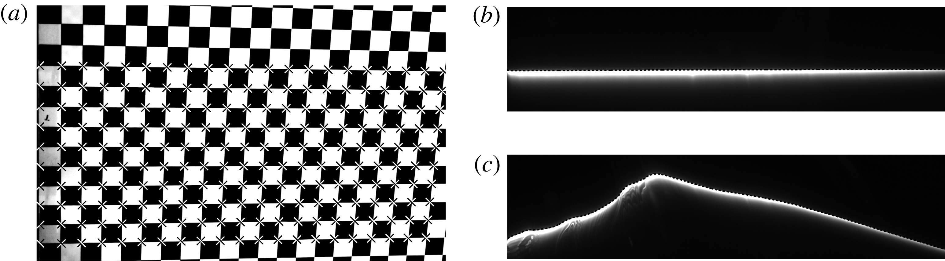
With the cameras having downward viewing angles, the subsurface water within the light sheet serves as the background illumination for the surface features between the light sheet and the cameras. These features can be seen in the LIF images and can be used for qualitative observations of the water surface behaviour. Within the plane of the light sheet, the water surface appears to be a sharp boundary where the intensity gradient reaches a local maximum. The surface profiles were extracted from the LIF images based on a method described in Liu & Duncan (Reference Liu and Duncan2006). A sample result is shown in figure 3(c).
Sample images of the camera calibration grid and the detection of the water surface profile. Photograph of the calibration grid is shown in (a). The extracted corner points are marked as black–white crosses. The grid is placed in the plane of the laser light sheet and the left edge of the grid is flush with the front face of the impact structure. Sample LIF images of the undisturbed water surface and the water surface during wave impact are shown in (b) and (c), respectively. The water surface profiles computed from these images are shown as dashed lines. In (b), the dashed line is the
 $x$
axis in the coordinate system used in this study, see figure 2.

Image distortions created by lens optics and the oblique view of the plane of the profile measurements, i.e. the plane of the light sheet, are corrected via images of a calibration board. The calibration board (
 $61~\text{cm}\times 61~\text{cm}$
) has a checker board pattern of black and white squares (
 $25.4~\text{mm}\times 25.4~\text{mm}$
) on its front surface. Before and after the measurements for each experimental condition, the calibration board is mounted on the structure so that its square-patterned surface is within the light sheet and the left edge of the board is flush with the front face of the structure. In this manner, the coordinates of the corners of the squares are known relative to the structure and the mean water level. Images of the calibration board are recorded by all cameras and a sample calibration image is shown figure 3(a). The calibration board is removed from the tank before the wave impact experiments are performed.
The images of the calibration board are processed to obtain the image coordinates of the corner points
 $(X_{I},Z_{I})$
, see figure 3(a). The coordinates of these corner points in the laboratory reference frame,
 $(X_{L},Z_{L})$
, are known relative to the front face of the structure and the mean water level, as mentioned above. It was found that the functions
 $X_{L}=f_{x}(X_{I},Z_{I})$
and
 $Z_{L}=f_{z}(X_{I},Z_{I})$
were accurately represented by third-order polynomials whose coefficients were determined by least-squares fit to the calibration data. Using these polynomials, the coordinates of all the points in the image can be converted to coordinates in the plane of the light sheet in the laboratory reference frame:
 $$\begin{eqnarray}\displaystyle & \displaystyle X_{L}(X_{I},Z_{I})=\mathop{\sum }_{m=0}^{3}\mathop{\sum }_{n=0}^{3}A_{mn}X_{I}^{m}Z_{I}^{n} & \displaystyle\end{eqnarray}$$
 $$\begin{eqnarray}\displaystyle & \displaystyle Z_{L}(X_{I},Z_{I})=\mathop{\sum }_{m=0}^{3}\mathop{\sum }_{n=0}^{3}B_{mn}X_{I}^{m}Z_{I}^{n}. & \displaystyle\end{eqnarray}$$
Before each experimental run, an LIF image of the still water surface was taken (see figure 3 b). The coordinates of the mean water line in the image reference frame were extracted from this image.
The coordinates (in the image reference frame) of the mean water line was first used in the above polynomial fitting functions to obtain the corrected coordinates (in the laboratory reference frame) of the mean water line. Then a linear function was fitted to the corrected water line to find its slope. The laboratory coordinate system was rotated to compensate for this slope so that in the rotated coordinate system, the mean water line is horizontal. The coordinates of the intersection of the mean water line and the front surface of the structure were found in the new coordinate system following the above procedures. Finally, the coordinate system was translated so that this intersection is at the origin.
2.4 Impact pressure measurements
The impact pressure on the front surface of the structure was measured. The measurement positions are along two vertical lines which are symmetric about the vertical centreline of the structure, shown in figure 2(b). The two vertical lines are 1.27 cm apart from each other. Similar to the experiments by Chan & Melville (Reference Chan and Melville1988), the measurement positions on the two lines are staggered in order to cover more vertical positions on the structure within the same range of heights. The vertical distance between two adjacent sensor positions on the same vertical line is 1.27 cm, so the smallest vertical spacing between sensors is 0.635 cm. There are 21 positions on one vertical line and 20 positions on the other, so that 41 different vertical positions can be measured.
A special hole profile for the pressure sensor was machined at each measurement position. The front plate of the cube is 1.905 cm thick. The hole profile was machined in a way such that the measurement plane of the sensor is recessed from the front face of the wall by 0.508 mm. This recess space was filled with insulating grease, which transmits the impact pressure to the pressure sensor as well as delays the possible thermal effect of the cold tank water when it comes in contact with the sensors that are initially above the mean water level.
The wave impact pressure was measured by piezoelectric pressure sensors (Part no.: 113B28) supplied by PCB Piezotronic Inc. The diameter of the sensor measurement face is 0.554 cm. The resolution, sensitivity and the measurement range of the pressure sensors are 0.007 kPa,
 $14.5~\text{mV}~\text{kPa}^{-1}$
and
 $\pm 344.7~\text{kPa}$
, respectively. The rise time of the sensor is less than
 $1~\unicode[STIX]{x03BC}\text{s}$
and its low-frequency response limit is 0.5 Hz. Twenty-four pressure sensors were used in this experiment simultaneously and 17 plugs were used to fill the other 17 holes. The mounting positions of sensors on the structure were changed when the height of the structure was varied.
The outputs from the pressure sensor signal conditioners were sent to an analogue-to-digital data acquisition system (National Instruments, Inc.). The system has 24 simultaneous-sample-and-hold input channels and each channel has a 14-bit resolution. The signal conditioners and data acquisition system were set to maximum sensitivity which corresponds to a minimum voltage step of 0.1526 mV and a minimum pressure step of 0.01 kPa. The sample rate used in the experiments ranges from 500 to 900 kHz and the duration of the pressure measurements was 0.75 s. The surface profile measurements and pressure measurements were synchronized with the wave maker motion by using a pulse-delay generator.
2.5 Experimental procedures and conditions
The following procedures were followed during the experiments. Before every experimental run, the wave maker wedge was raised to its equilibrium position and kept stationary for at least 30 min before measurements. As a result, the surface disturbances generated when raising the wedge were damped out. When the wedge was at its equilibrium position just before the measurements, an LIF image of the quiescent water surface was recorded by each camera. The mean water level line was extracted from these images and was defined as the
 $x$
-axis (
 $z=0$
) in the analysis, as described in § 2.3. The tank’s quiescent water level was monitored by a forth camera (resolution 30 pixels per mm) to ensure the water level consistency throughout all conditions with an error less than 0.2 mm. During the wave maker motion, in order to avoid electrical noise from the servo-motor that might affect the pressure signal, the wave maker was turned off just before the wave impact. After the impact, the fans and the water filtration system were turned on for approximately 15 min. After the fans and filtration system were turned off, the wave maker wedge was again raised to its equilibrium position for the next run. The surface tension of the water in the tank was monitored and measured with a Wilhelmy plate before the first run and after the last run of each day. The surface tension maintained values very close to that of clean water at room temperature,
 $73\pm 0.5~\text{dyne}~\text{cm}^{-1}$
.
In the current experiments, the structure was located at a single streamwise position along the tank, with its front face 641.5 cm (
 $5.43\unicode[STIX]{x1D706}_{0}$
) from the back face of the wave maker. The vertical position of the bottom of the structure,
 $z_{b}$
, where
 $z=0$
is the mean water level and positive
 $z$
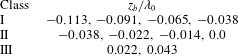
is up, was located at 9 positions as given in table 1. Three response classes are identified in the table and are described in more detail in the following section. The wave maker motion given by (2.1) was used for all conditions.
Values of
 $z_{b}/\unicode[STIX]{x1D706}_{0}$
for the experimental conditions in each class of water surface behaviour. Class I: the bottom of the structure remains submerged during the entire impact process. Class II: the bottom of the structure transitions from submerged to airborne at least once during the impact process. Class III: the bottom of the structure is initially above the water surface and only makes contact with the main wave crest. The condition
 $z_{b}/\unicode[STIX]{x1D706}_{0}=-0.038$
is listed in both class I and class II because, although the bottom of the structure remains submerged throughout the impact process (class I), the physical behaviour of the free surface is similar to that found in class II.

One can consider these experiments to be a Froude scaled model for a larger-scale prototype wave–structure interaction. In this Froude scaling, the effects of viscosity as defined by the Reynolds number and surface tension as defined by the Weber number do not scale. The present experiments with a
 $Re=\overline{c}_{p}L/\unicode[STIX]{x1D708}=3.6\times 10^{5}$
, where
 $L$
is the thickness of the structure (
 ${\approx}30~\text{cm}$
), and with the sharp corners at the bottom edge of the structure should be a fairly good approximation for larger-scale devices. Surface tension effects control capillary wave generation at the contact line and fine-scale features like droplets and air bubbles generated at the wave crest. In a larger-scale prototype, the ratio between the gravity wavelength and the capillary wavelength will grow and effects like the capillary wave phenomena described is § 4.3, which will remain at millimetre length scales, will become less important. Also, the bubbles and droplets are expected to be smaller and more numerous and in larger-scale wave–structure interactions.
3 Results
The surface profile and pressure measurements are presented below in three subsections. In the following § 3.1, the profile history of the wave generated by the above-described wave maker motion operating in open water, i.e. with the structure removed from the wave tank, is presented. This is followed, in §§ 3.2 and 3.3, by presentations of the water surface profile histories and wall pressure measurements during the wave impact on the structure, respectively.
3.1 Wave behaviour in open water
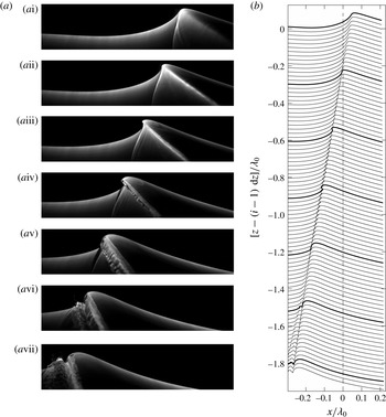
In order to show how the breaker is affected by the structure, the surface profile history of the breaker was first measured in open water. Images and surface profiles from an LIF movie of the open-water breaker are shown in 4(a) and 4(b), respectively. In the first image (i) and corresponding profile, the front (left) face of the wave near the crest is nearly vertical, indicating that the jet is about to form. Tracking the speed of the highest point of the crest region in this early phase of breaking yields a crest speed of
 $1.5~\text{m}~\text{s}^{-1}$
which is a little greater than the average linear theory phase speed of the 32 wave components of the packet,
 $\overline{c}_{p}=1.437~\text{m}~\text{s}^{-1}$
. As the sequence progresses, the tip of the jet becomes visible and moves horizontally (ii and iii). The jet tip then falls downward (iv and v) and plunges into the water surface (vi) downstream (to the left) of the crest. This impact generates a zone of rough water surface downstream of the jet impact site (vii). The plunging breaker has a moderate strength in that, for a stronger breaker, the jet impact site would be farther downstream from the crest. The largest crest height during the breaking process was
 $H_{m}=10.1~\text{cm}$
as measured from the mean water level.
Images and profiles of the plunging breaker in the absence of the structure. The breaker is travelling from right to left. (a) Sequence of LIF images from a high-speed movie of the breaker. The imaged area is 63 cm by 15 cm and the time interval between successive images is 47 ms (
 $=0.0541/f_{0}$
). The sharp boundary between the upper dark region and the lower bright region is the water surface profile in the plane of the light sheet. The lower bright region is illuminated by the fluorescing dye in the subsurface water within the light sheet. (b) Surface profile history of the plunging breaker taken from the same movie as the images in (a). The time between profiles is 3.3 ms (
 $=0.0038/f_{0}$
) and each subsequent profile is plotted
 $\text{d}z=0.022\unicode[STIX]{x1D706}_{0}$
below the previous profile. The profiles corresponding to the images in (a) are plotted in bold. The dashed line (
 $x/\unicode[STIX]{x1D706}_{0}=0$
) is the position of the front face of the structure in the experiments described in §§ 3.2 and 3.3. The movie from which these images were taken is available as supplementary material, filename: Movie 1.mp4.

In the wave impact experiments, the front face of the structure was placed at the position of the dashed line in figure 4(b). At this position, in open water, the jet has just started to form and is moving horizontally. As is shown in following subsection, this behaviour is dramatically changed by the presence of the structure.
3.2 Water surface evolution during impact
In this subsection, the water surface profile evolution during wave impact on the structure is discussed. The presentation is organized into three subsections according to the general class of behaviour of the water surface near the bottom of the structure: Response class I, defined as cases in which the bottom surface of the structure is initially below mean water level and remains submerged during the impact, is discussed in § 3.2.1. Response class II, defined as cases in which the bottom of the structure is near the mean water level and transitions back and forth from above to below the instantaneous local water level at least once during the impact process, is discussed in § 3.2.2. Finally, response class III, defined as cases in which the bottom of the structure is well above the mean water level and only the wave crest hits the structure, is discussed in § 3.2.3. The values of
 $z_{b}/\unicode[STIX]{x1D706}_{0}$
corresponding to each of these response classes are given in table 1.
3.2.1 Class I. The bottom of the structure remains submerged
When the bottom of the structure is positioned at
 $z_{b}=-0.113\unicode[STIX]{x1D706}_{0}$
,
 $-0.091\unicode[STIX]{x1D706}_{0}$
,
 $-0.065\unicode[STIX]{x1D706}_{0}$
and
 $-0.038\unicode[STIX]{x1D706}_{0}$
, it remains submerged during the entire wave impact process. A flip-through response (defined below) occurs for the three deepest submergence cases and these will be discussed in this section. As the submergence (defined as
 $|z_{b}|$
for
 $z_{b}\leqslant 0$
) is decreased, ripples generated at the contact line on the front face of the structure become stronger and seem to interfere with the flip-through process in the
 $z_{b}=-0.038\unicode[STIX]{x1D706}_{0}$
case. For this reason the data from the
 $z_{b}=-0.038\unicode[STIX]{x1D706}_{0}$
case are presented along with the class II cases where the ripple effect is even stronger. In the following, the data from the condition with the largest submergence (
 $z_{b}=-0.113\unicode[STIX]{x1D706}_{0}$
) are discussed in detail while selected quantities from all three data sets are compared to explore the effect of the submergence on this class of impact.
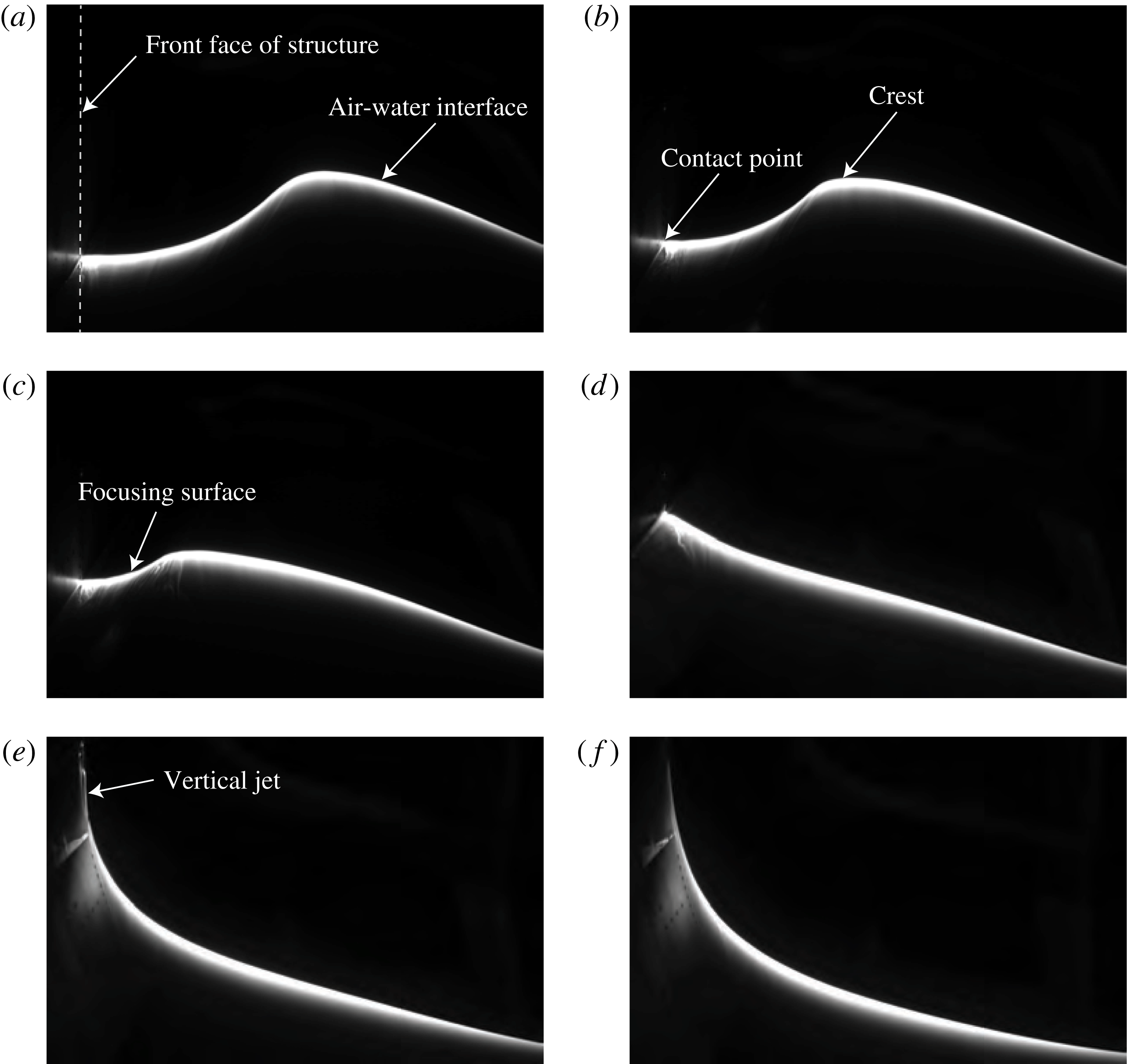
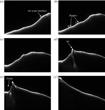
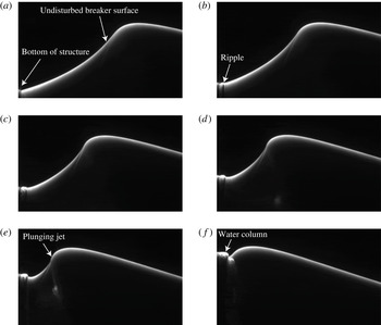
A sequence of images from a high-speed LIF movie of the evolution of the water surface profile for
 $z_{b}=-0.113\unicode[STIX]{x1D706}_{0}$
. The field of view is approximately
 $55~\text{cm}\times 36~\text{cm}$
. The location of the front face of the structure and various features of the water surface profile are shown on the figure. The contact point is located at the left of the images and is defined at the intersection of the instantaneous water surface in the plane of the laser light sheet and the front surface of the structure. The images were recorded at 500 f.p.s. and from (a) to (f), the images were taken at
 $tf_{0}=-0.173$
,
 $-0.115$
,
 $-0.058$
, 0.0,
 $0.058$
, 0.115, respectively. Panel (d) shows the moment of impact (see text for discussion) and this time is taken as
 $t=0$
. The movie from which these images were taken is available as supplementary material, filename: Movie 2.mp4.

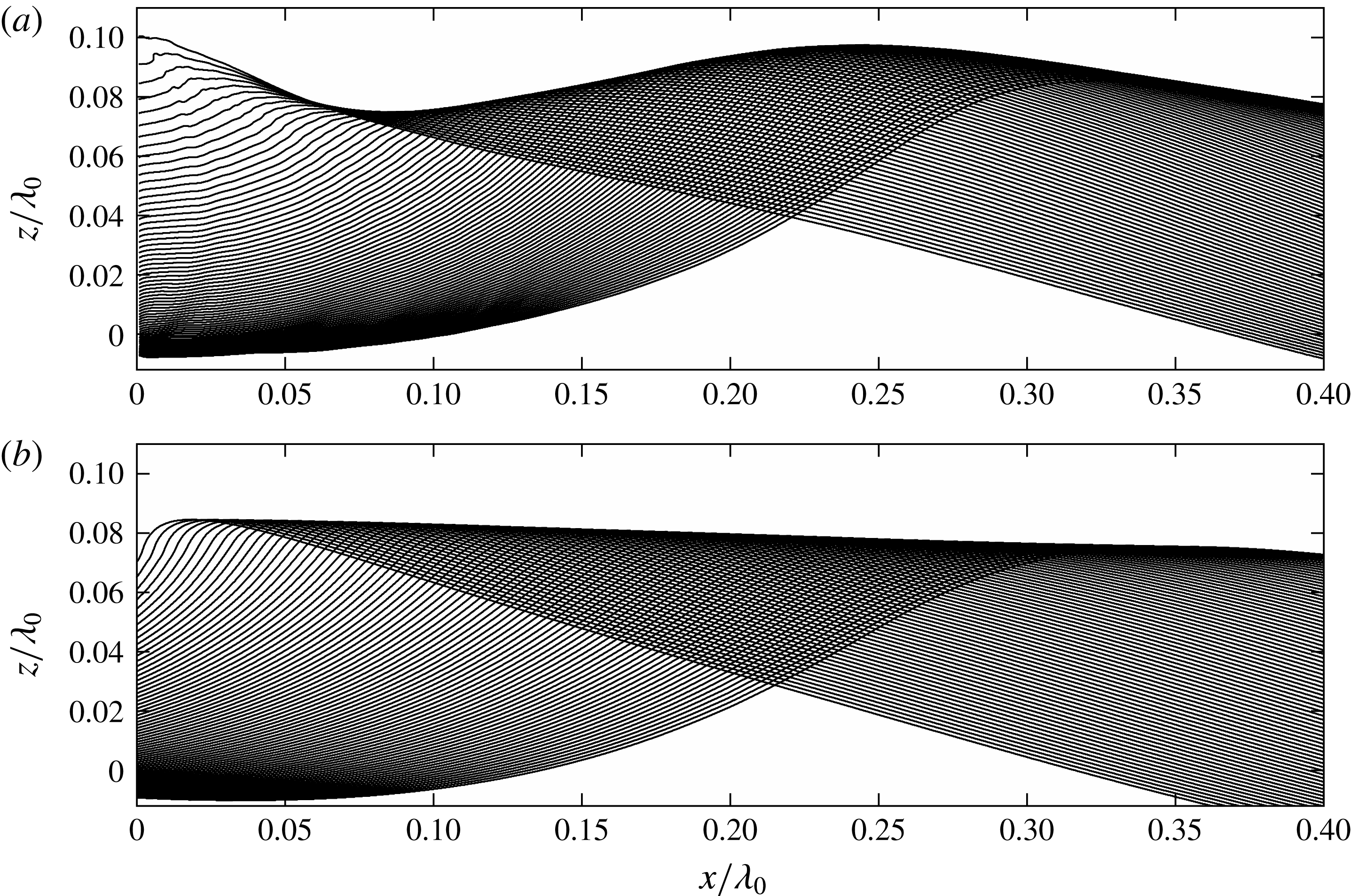
Surface profile histories plotted in the laboratory reference frame for (a) condition
 $z_{b}=-0.113\unicode[STIX]{x1D706}_{0}$
and (b) the breaker in open water. In both panels, the time between profiles is 3.3 ms (
 $=0.00380/f_{0}$
) and the total time covered is 264 ms (
 $=0.3036/f_{0}$
). In (a), the last profile plotted corresponds to nearly the moment of impact. In (b), the last profile plotted corresponds to the instant when the vertical surface of the open-water wave crest reaches the streamwise position (
 $x/\unicode[STIX]{x1D706}_{0}=0$
) of the front face of the structure in (a). The mean water level is at
 $z/\unicode[STIX]{x1D706}_{0}=0$
.

Images from an LIF movie for
 $z_{b}=-0.113\unicode[STIX]{x1D706}_{0}$
are shown in figure 5. As the crest approaches the wall, the water surface between the contact point on the front face of the structure and a point just downstream (to the left) of the crest point forms an arc with upward curvature, herein called the ‘focusing surface’, see figure 5(c). Further upstream, the crest region, which has downward curvature, merges to the back face of the wave, which forms a nearly straight line. As the impact continues, panels (b) through (d), the crest moves downstream, the arc between the crest and the contact point shrinks and the slope of the back face of the wave remains nearly constant. In panel (d), the arc between the contact point and the crest has focused to a point and the entire water surface has become a nearly straight line, except for a small portion upstream of the contact point which has a slightly larger slope than the rest of the surface. This instant in time is defined herein as the moment of impact. Shortly after the moment of impact, a high-speed thin vertical jet is initiated and grows upward along the surface of the structure under the effects of gravity and friction from the wall, see panels (e) and (f). Following the nomenclature from Peregrine (Reference Peregrine2003), we call this type of impact, flip through.
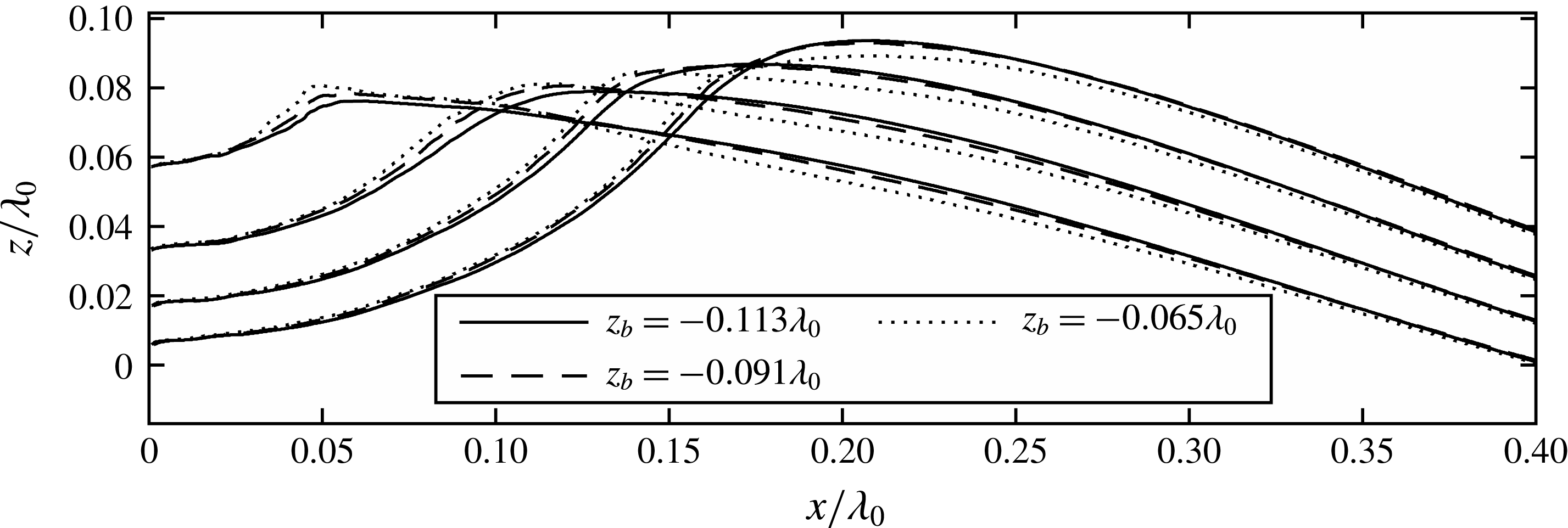
Surface profiles at four times for three values of
 $z_{b}$
in Class I. The time interval between successive profiles is 33.3 ms (
 $=0.0383/f_{0}$
).

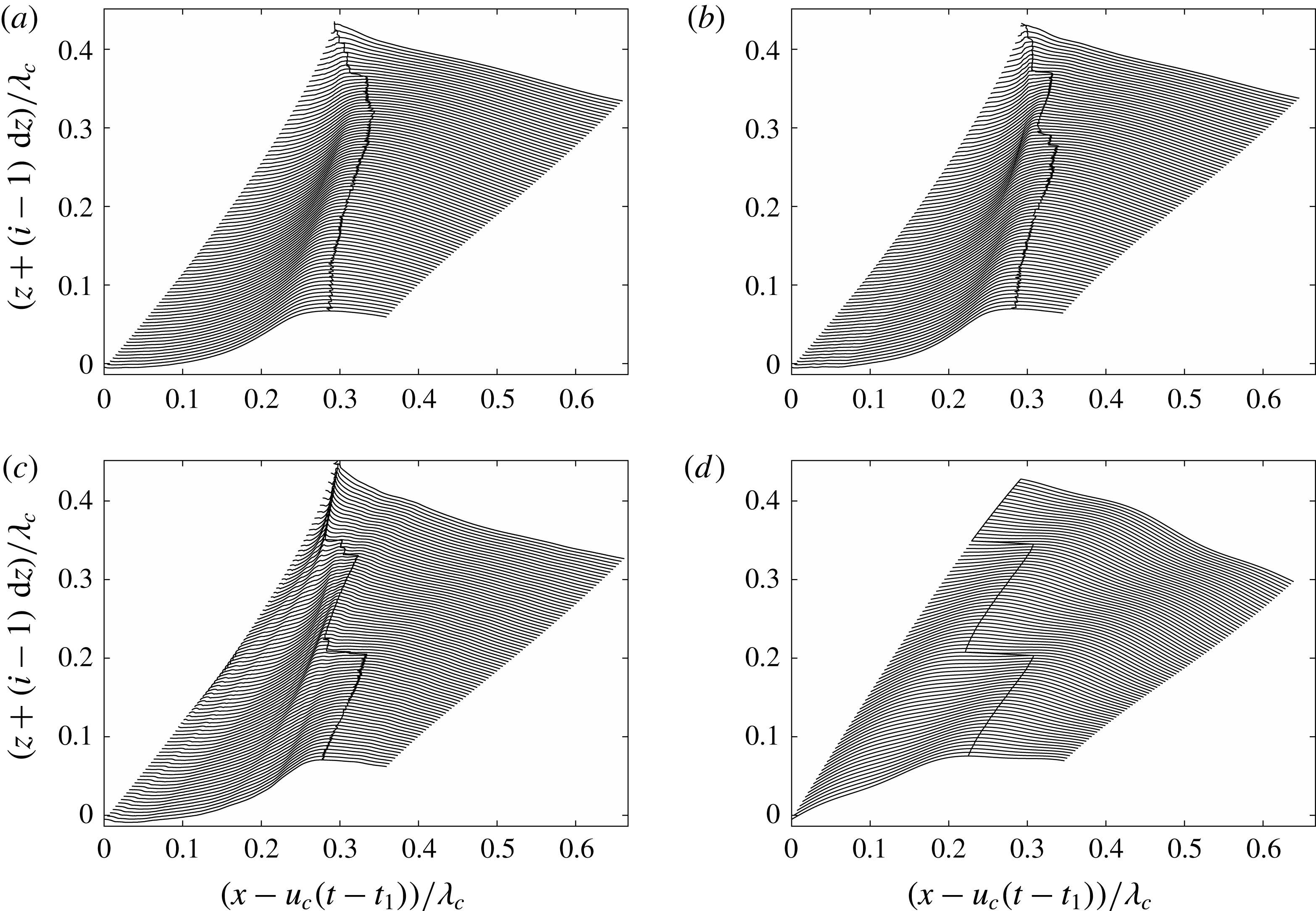
A set of surface profiles corresponding to the high-speed movie from which the images in figure 5 were taken are shown in figure 6(a). The profile sequence is plotted in the laboratory reference frame and ends at the moment of impact. For comparison, a set of profiles of the wave in open water and plotted in the same reference frame are given in figure 6(b). In the wave impact case, the profiles upstream of the crest are nearly parallel straight lines that are tilted clockwise by about
 $\unicode[STIX]{x1D703}_{0}=13.6^{\circ }$
from the horizontal. The parallel lines are nearly equally spaced by 0.0043 m horizontally, which indicates the upstream surface of the wave is moving horizontally at a nearly constant velocity of
 $0.9\bar{c}_{p}$
. It can also be seen that as the crest point travels toward the structure, its absolute height first decreases and then increases as the moment of impact is approached. The wave in open water moves downstream at a nearly constant speed of
 $1.044\bar{c}_{p}$
and with a continually increasing amplitude at this position in the tank.
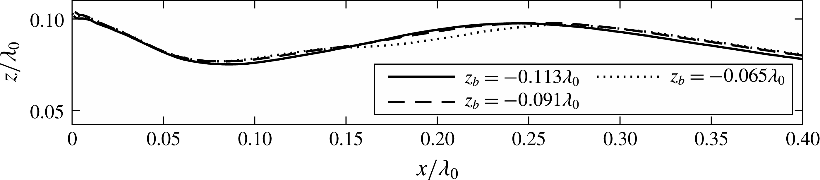
The flip-through behaviour occurs at all three wall submergences in this response class, but there are quantitative differences in the profile histories. To illustrate these differences, a limited set of surface profiles for each of the three submergence conditions are shown in figure 7. The four profiles for
 $z_{b}=-0.113\unicode[STIX]{x1D706}_{0}$
are taken at 33.3 ms (
 $=0.0383/f_{0}$
) intervals starting 130 ms (
 $=0.1495/f_{0}$
) before the moment of impact. In order to allow direct comparisons of the profile shapes, the profiles for the
 $z_{b}=-0.091\unicode[STIX]{x1D706}_{0}$
and
 $-0.065\unicode[STIX]{x1D706}_{0}$
cases are at times when the contact points on the structure are at the same locations as in the profiles for the
 $z_{b}=-0.113\unicode[STIX]{x1D706}_{0}$
case. The time changes needed to match the contact point heights with the
 $z_{b}=-0.113\unicode[STIX]{x1D706}_{0}$
case are approximately 2.7 ms (
 $=0.00311/f_{0}$
later) for the
 $z_{b}=-0.091\unicode[STIX]{x1D706}_{0}$
case and 5.4 ms (
 $=0.00621/f_{0}$
later) for the
 $z_{b}=-0.065\unicode[STIX]{x1D706}_{0}$
case. As can be seen from the figure, the general behaviour of the profiles at all three submergences (
 $|z_{b}|$
) is quite similar. In the region downstream of the crest, the water surface height at any streamwise position increases slightly as the submergence increases. However, on the upstream side of the crest, the opposite trend is found. It can also be seen that the crest point height increases and shifts slightly downstream with increasing submergence.
The top envelopes of the surface profiles at times before the moment of impact for three submergence cases with flip-through behaviour, class I impact.

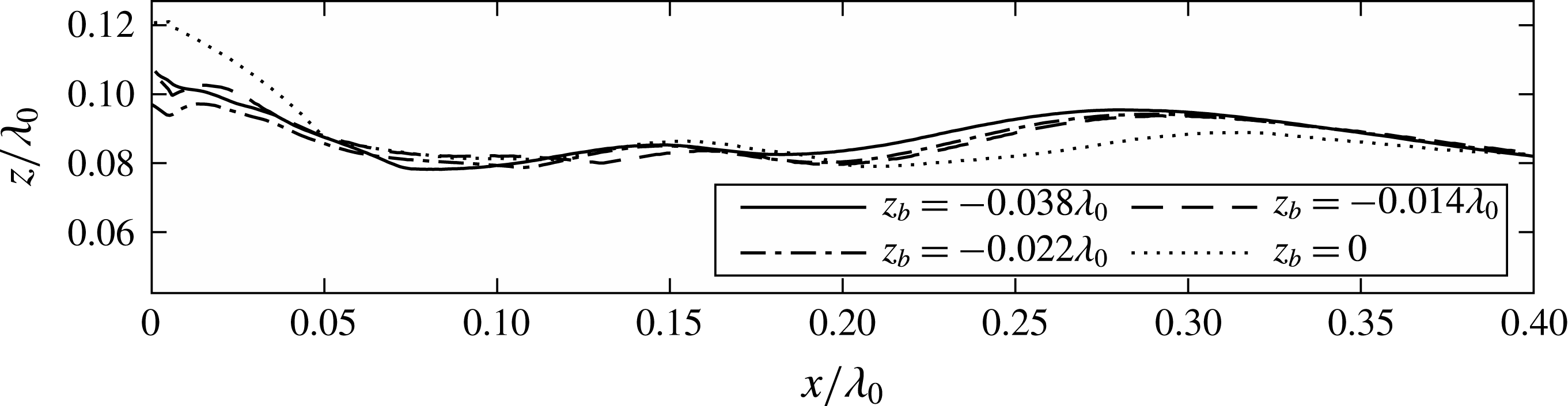
Another interesting feature that can be used to compare the behaviour of the wave surface evolution is the top envelope lines of all surface profiles at each submergence, as shown in figure 8. At each streamwise position, a point above this line is always in the air while a point below this line is at least for a moment in the water. For all three conditions, the envelope lines show two peaks and one trough within the range of the plot. The envelopes for the
 $z_{b}=-0.113\unicode[STIX]{x1D706}_{0}$
and
 $-0.091\unicode[STIX]{x1D706}_{0}$
cases are quite similar, though the downstream trough and the upstream crest positions are slightly shifted in
 $x$
. The envelope for the
 $z_{b}=-0.065\unicode[STIX]{x1D706}_{0}$
in the range
 $0.15<x/\unicode[STIX]{x1D706}_{0}<0.25$
has a different shape than the other two curves. Some aspects of these features of the envelope profiles are discussed in § 4.3.
3.2.2 Class II. Interaction between the bottom of the wall and the water surface
In this subsection, surface profile results are presented for conditions with
 $z_{b}=-0.038\unicode[STIX]{x1D706}_{0}$
,
 $z_{b}=-0.022\unicode[STIX]{x1D706}_{0}$
,
 $z_{b}=-0.014\unicode[STIX]{x1D706}_{0}$
,
 $z_{b}=0$
. At conditions
 $z_{b}=-0.022\unicode[STIX]{x1D706}_{0}$
,
 $z_{b}=-0.014\unicode[STIX]{x1D706}_{0}$
,
 $z_{b}=0$
, small-amplitude waves that arrive at the structure before the main crest arrives cause the bottom of the structure to be exposed to air and then re-enter the water for one or more cycles. As described above, at the condition
 $z_{b}=-0.038\unicode[STIX]{x1D706}_{0}$
, the bottom of the wall remains submerged throughout the impact process; however, as in the other three cases, disturbances generated at the contact line on the front face of the structure propagate to the incoming main wave crest and affect its behaviour in a similar way. In the following, the condition
 $z_{b}=0$
will be discussed in detail and some comparisons of profile features will be made among all the four conditions.
A sequence of images from an LIF movie showing the evolution of the water surface for
 $z_{b}/\unicode[STIX]{x1D706}_{0}=0$
. The contact point is located at the left of the images. The images were recorded at a frame rate of 4500 Hz, but in the images shown here, the time interval between two successive frames is 21.3 ms (
 $=0.02450/f_{0}$
). The field of view is approximately
 $18~\text{cm}\times 13~\text{cm}$
. The movie from which these images were taken is available as supplementary material, filename: Movie 3.mp4.

Surface profile history for condition
 $z_{b}=0$
in a reference frame fixed in the laboratory. The time between profiles is 3.3 ms (
 $=0.00380/f_{0}$
). The profiles are plotted from
 $tf_{0}=-0.3228$
(281 ms) to the moment of impact (
 $tf_{0}=0$
).

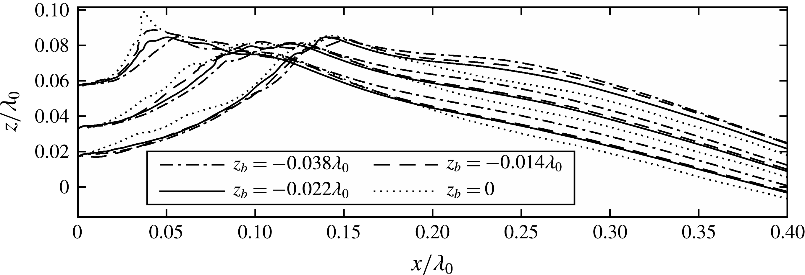
Surface profiles at three times for four values of
 $z_{b}$
. The impacts for
 $z_{b}=-0.022\unicode[STIX]{x1D706}_{0}$
,
 $-0.014\unicode[STIX]{x1D706}_{0}$
and
 $0.0$
are categorized as class II. For reasons discussed in § 3.2.1, the curves for
 $z_{b}=-0.038\unicode[STIX]{x1D706}_{0}$
are plotted as well.

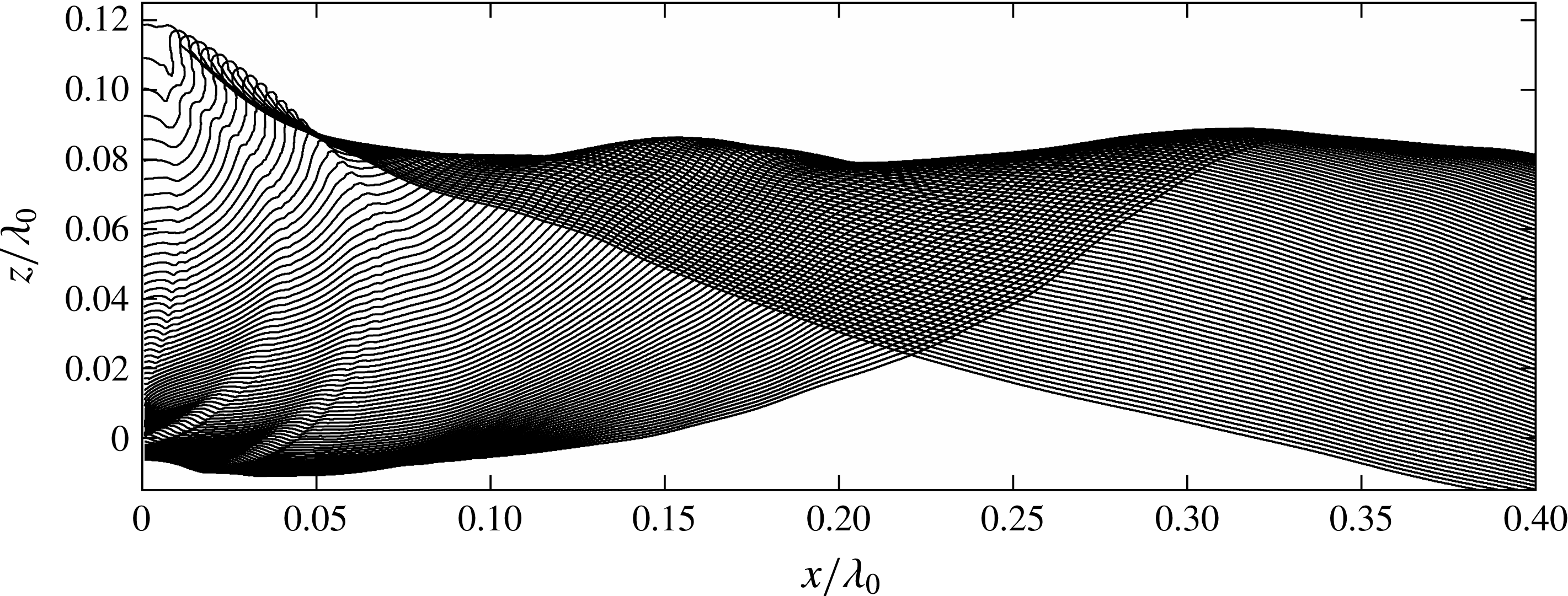
Figure 9 shows six images from a high-speed movie of the evolution of the water surface for the
 $z_{b}/\unicode[STIX]{x1D706}_{0}=0$
case and a set of surface profiles from the same movie are shown in figure 10. As is shown in § 4.3, before the main crest arrives at the wall, small-amplitude wave components in the dispersive wave packet arrive and interact with the bottom of the wall. This interaction creates ripples at the free surface and these ripples propagate upstream, toward the wave maker. Two of these ripples are identified in panel (b) of figure 9. At the same time, the large-amplitude main crest approaches the wall and the small ripples are confined within the profile segment with upward curvature between the front surface of the structure and the crest. The ripples propagate along this curved surface and merge with each other as the surface segment shrinks. This process is most clearly seen in the profiles in figure 10. The merged ripples grow in amplitude and turn into the jet that forms at the crest of the wave. As the process continues, the crater between the jet and the wall shrinks in size and the contact point moves rapidly upward. The contact point reaches the height of the jet tip before the jet tip reaches the wall. Therefore, the jet impacts on a water column rather than the wall and appears to enclose an air pocket.
Surface profiles at three times in the impact process for all four submergence conditions are compared in figure 11. As in figure 7, the times are adjusted slightly so that the contact point height is the same for each set of four curves. At the instants plotted, the surface height at the same streamwise position between the contact point and the crest is larger for conditions with smaller submergences and this difference is more significant at later time. The surface profiles become more rough for conditions with smaller submergences, indicating that the disturbances generated at the contact point are stronger. Compared with the flip-through conditions shown in figure 7, the surface profile upstream of the crest region in these four conditions is less straight. Also, unlike the flip-through conditions where the crest is the only local maxima, the crest regions in the present cases have a main peak and several nearby local maxima. From the corresponding movies, it can be seen that these local maxima are due to the evolution of upstream-propagating disturbances as discussed in § 4.3. The multiple peaks of the crest region are also seen in the top envelops of the surface profiles in figure 12. The envelope for the
 $z_{b}=0$
condition has a steep rise in the range of
 $0<x/\unicode[STIX]{x1D706}_{0}<0.05$
; this is caused by the jet generated at the crest as the jet merges with the ripples from the contact point.
3.2.3 Class III. Impact when the bottom of the structure is above the mean water level
If the bottom of the structure is sufficiently above the mean water level to allow the small wave components that arrive before the main wave crest to pass downstream undisturbed, only the main crest interacts with the front face of the structure. The two conditions (
 $z_{b}/\unicode[STIX]{x1D706}_{0}=0.022$
and
 $z_{b}/\unicode[STIX]{x1D706}_{0}=0.043$
) in this class are discussed below.
The top envelopes of the surface profiles at times before the moment of impact for four submergence cases when the bottom of the wall interacts with the water surface. The cases for
 $z_{b}=-0.022\unicode[STIX]{x1D706}_{0}$
,
 $-0.014\unicode[STIX]{x1D706}_{0}$
and
 $0.0$
are categorized as class II impacts. For reasons discussed in § 3.2.1, the curve for
 $z_{b}=-0.038\unicode[STIX]{x1D706}_{0}$
is plotted as well.

Sequence of LIF images of the water surface profile for
 $z_{b}/\unicode[STIX]{x1D706}_{0}=0.022$
. The images were recorded at a frame rate of 4500 Hz, but in the images shown here, the time interval between two successive frames is 13.3 ms (
 $=0.01530/f_{0}$
). The field of view is approximately
 $18~\text{cm}\times 16~\text{cm}$
. The movie from which these images were taken is available as supplementary material, filename: Movie 4.mp4.

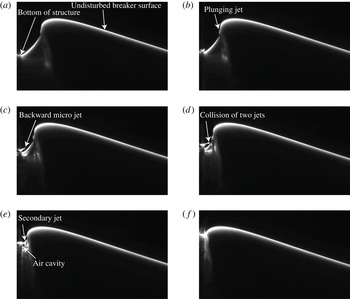
Sequence of LIF images of the water surface profile for
 $z_{b}/\unicode[STIX]{x1D706}_{0}=0.043$
. The images were recorded at a frame rate of 4500 Hz, but in the images shown here, the time interval between two successive frames is
 $3.1~\text{ms}$
(
 $=0.00357/f_{0}$
). The field of view is approximately
 $18~\text{cm}\times 16~\text{cm}$
. The movie from which these images were taken is available as supplementary material, filename: Movie 5.mp4.

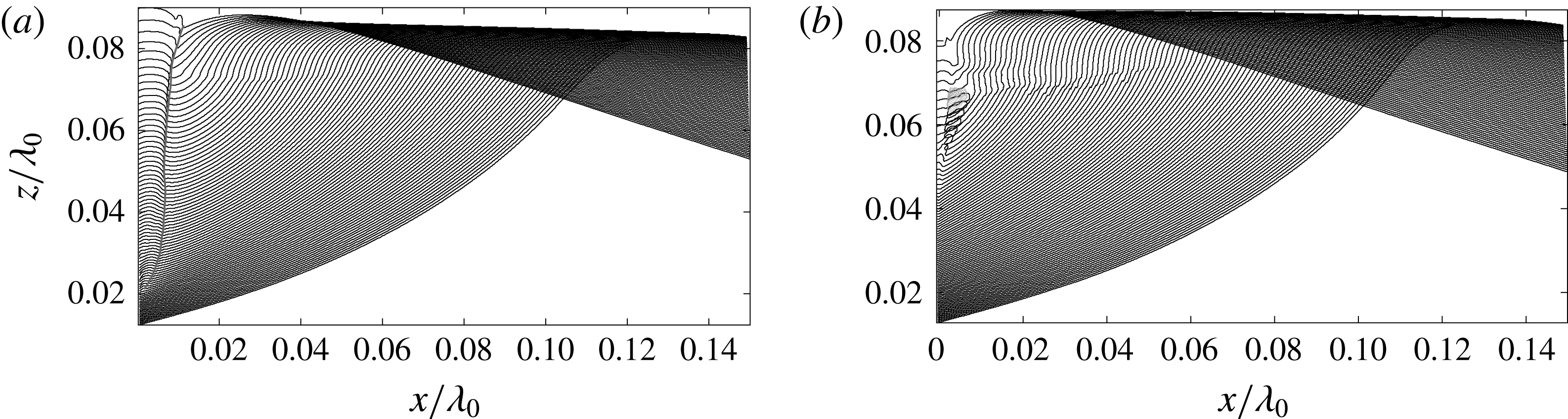
Surface profile histories (black lines) plotted in a laboratory-fixed reference frame for (a)
 $z_{b}=0.022\unicode[STIX]{x1D706}_{0}$
and (b)
 $z_{b}=0.043\unicode[STIX]{x1D706}_{0}$
. The time interval between two successive profiles is 1.11 ms (
 $=0.001277/f_{0}$
). In (a), the grey solid line represents the trajectory of the upstream trough of the ripple generated along the wall. In (b), the grey solid lines are the boundaries of the air cavity at several times when it is visible in the LIF movies after the micro-jet meets the plunging jet. Since the air cavity is observed through the water free surface, the boundaries are only approximate.

Figure 13 shows a sequence of LIF images of the water surface evolution of the case
 $z_{b}/\unicode[STIX]{x1D706}_{0}=0.022$
and a set of surface profiles from the same high-speed movie are shown in figure 15(a). In 13(a), the water surface is about to make first contact with the structure and this ‘undisturbed’ profile is the same as in the open-water case. As the process continues, the downstream side of the breaker first hits the front lower corner of the structure, see panel (b). Then the bottom and front face of the structure block the motion of the water and cause the formation of a ripple. As the process continues, the ripple grows in size, see panels (c) and (d). Eventually the ripple grows into a thick water column that moves upward. It is noted that even though the structure blocks some of the flow, the plunging jet begins to form, see panel (e), as it would in open water. However, in the present case the jet formation is blocked by the large water column on the front face of the structure, see panel (f). These features are shown clearly in the profile history in figure 15(a).
Images from a high-speed movie of the wave impact for the highest position of the structure (
 $z_{b}/\unicode[STIX]{x1D706}_{0}=0.043$
) are shown in figure 14 and a set of surface profiles from the same movie are shown in figure 15(b). In figure 14(a), the wave crest has not yet hit the structure so the breaker is as it would be in open water. Because the bottom surface of the structure is higher than in the
 $z_{b}/\unicode[STIX]{x1D706}_{0}=0.022$
case, the breaker for the
 $z_{b}/\unicode[STIX]{x1D706}_{0}=0.043$
case has more time to propagate in an open-water condition and the plunging jet is more pronounced just before impact, compare panels 13(a) and 14(a). As the impact process begins (panel (b)), a micro-jet forms near the contact point (see panels (b) and (c)), rather than the large ripple formed in the
 $z_{b}/\unicode[STIX]{x1D706}_{0}=0.022$
case. The micro-jet grows toward the upstream direction within the small space between the front face of the structure and the breaker’s plunging jet (panels (c) and (d)). Once the micro-jet reaches the plunging jet, the collision between the two jets creates a secondary jet that moves downstream (e). The secondary jet hits the rising water column along the front face of the wall. Finally, the breaker’s plunging jet hits the water column rising along the wall, making it highly likely that air is entrained during this process (f).
3.3 Impact pressure
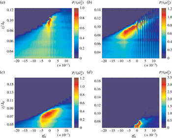
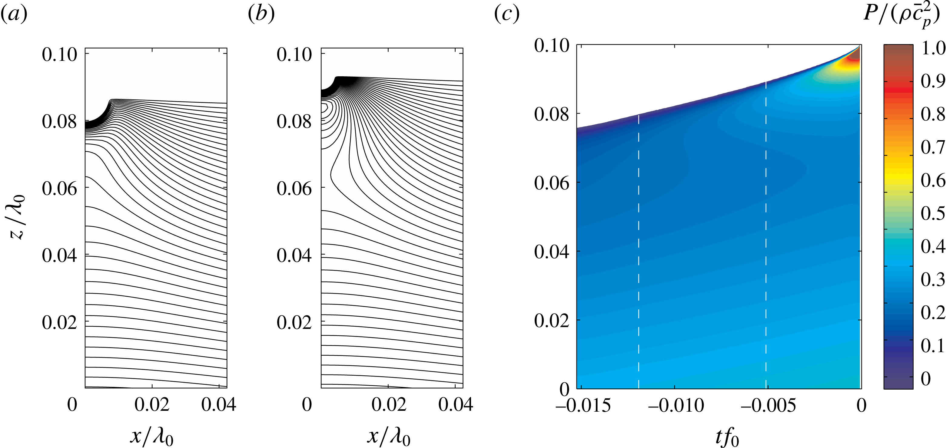
The temporal evolution of the wall pressure distribution for wave impacts for
 $z_{b}=-0.113\unicode[STIX]{x1D706}_{0}$
,
 $0.0$
,
 $0.022\unicode[STIX]{x1D706}_{0}$
and
 $0.043\unicode[STIX]{x1D706}_{0}$
are presented in this subsection. For each value of
 $z_{b}$
, the pressure is displayed as a contour plot on a
 $z$
–
 $t$
plane, see figure 16. The time histories of the pressures measured by different sensors at corresponding conditions can be found in figure B.1 in Wang (Reference Wang2017). Figure 16(a) corresponds to
 $z_{b}=-0.113\unicode[STIX]{x1D706}_{0}$
, which is the flip-through case for which images of the free surface were presented in figure 5. At each instant in time, the boundary between the upper dark blue region and the region below in figure 16(a) is the approximate location of the water surface. The free surface height and the vertical pressure gradient just below the free surface increase with time. The step-like structure of the boundary at the free surface is due to the finite size and discrete locations of the pressure sensors. At approximately
 $tf_{0}=-0.002$
, a double pressure spike of magnitude near
 $2.7\unicode[STIX]{x1D70C}\bar{c_{p}}^{2}$
appears just under the free surface. Each spike lasts for approximately
 $\unicode[STIX]{x0394}tf_{0}=0.002$
and has a vertical extent of
 $\unicode[STIX]{x0394}z=0.01\unicode[STIX]{x1D706}_{0}$
. The physics underlying the various features of the impact pressure will be further discussed in § 4.2.
Wall pressure distributions for
 $z_{b}/\unicode[STIX]{x1D706}_{0}=-0.113$
,
 $0.0$
,
 $0.022$
and
 $0.043$
are shown as pressure contours on the
 $z$
–
 $t$
plane in panels (a), (b), (c) and (d), respectively. Each plot is the measurement from one typical run. The magnitude of the pressure is scaled by the nominal dynamic pressure
 $\unicode[STIX]{x1D70C}\bar{c_{p}}^{2}$
. The scale of the colour bar is varied because the range of impact pressures varies considerably from one condition to another. The height of the mean water level is
 $z/\unicode[STIX]{x1D706}_{0}=0$
. In the surface profile analysis of the flip-through case (§ 3.2.1), the time
 $tf_{0}=0$
was taken as the moment of impact defined according surface profile shape; however, here with the multiple impact modes at the various
 $z_{b}$
values,
 $tf_{0}=0$
is taken more generally as the time when the pressure reaches its maximum value.

At
 $z_{b}=0.0$
, as shown in figure 16(b), the high-pressure region along the wall spans over a much wider range of height and time than in 16(a): the spatial and temporal range where the pressure exceeds
 $1.0\unicode[STIX]{x1D70C}\bar{c_{p}}^{2}$
reaches approximately
 $0.03\unicode[STIX]{x1D706}_{0}$
and
 $0.009f_{0}^{-1}$
, respectively. The peak pressure is about
 $2.0\unicode[STIX]{x1D70C}\bar{c_{p}}^{2}$
. Pressure oscillations are observed at this condition. The oscillation of impact pressure occurs over the whole measurement range below the water surface. In the range of approximately
 $tf_{0}=0.0{-}0.005$
, the sensors at all heights have similar in-phase oscillations with frequency of approximately 1000 Hz. In the time span just after
 $tf_{0}=0.005$
, the oscillation frequency increases with time at the pressure sensors with higher positions, while the oscillation amplitude of these high-frequency components attenuates rapidly. At later times, the oscillation frequency measured by the top 5 sensors can reach as high as 2800 Hz. However, these high-frequency oscillations at later times are not picked up by the pressure sensors at the lower positions. The lower-frequency component (approximately 1000 Hz) lasts for a longer time at lower positions, even though the amplitude of this oscillation also damps over time.
The pressure contour plots for the two cases with
 $z_{b}>0.0$
are significantly different than those for the above discussed cases. At
 $z_{b}=0.022\unicode[STIX]{x1D706}_{0}$
, as shown in figure 16(c), the region of high pressure has a broad span with magnitude
 $0.8\unicode[STIX]{x1D70C}\bar{c_{p}}^{2}$
in both height (
 $\unicode[STIX]{x0394}z=0.03\unicode[STIX]{x1D706}_{0}$
) and time (
 $\unicode[STIX]{x0394}t=0.01f_{0}^{-1}$
), similar to the
 $z_{b}=0.0$
case (figure 16
b) for
 $tf_{0}<0.0$
. Peak pressures with the value of approximately
 $1.1\unicode[STIX]{x1D70C}\bar{c_{p}}^{2}$
are measured by multiple pressure sensors; however, no obvious pressure oscillation is found. At
 $z_{b}=0.043\unicode[STIX]{x1D706}_{0}$
, very high impact pressures and pressure oscillations are observed, as shown in figure 16(d). The peak pressure of this condition reaches as high as
 $4.5\unicode[STIX]{x1D70C}\bar{c_{p}}^{2}$
. The oscillation frequency is found to be higher than 3000 Hz, which is higher than that in the
 $z_{b}=0$
condition; however, the amplitude of the oscillation is significantly smaller than in the
 $z_{b}=0$
case.
4 Discussion
4.1 Properties of the focusing surface in flip-through impact
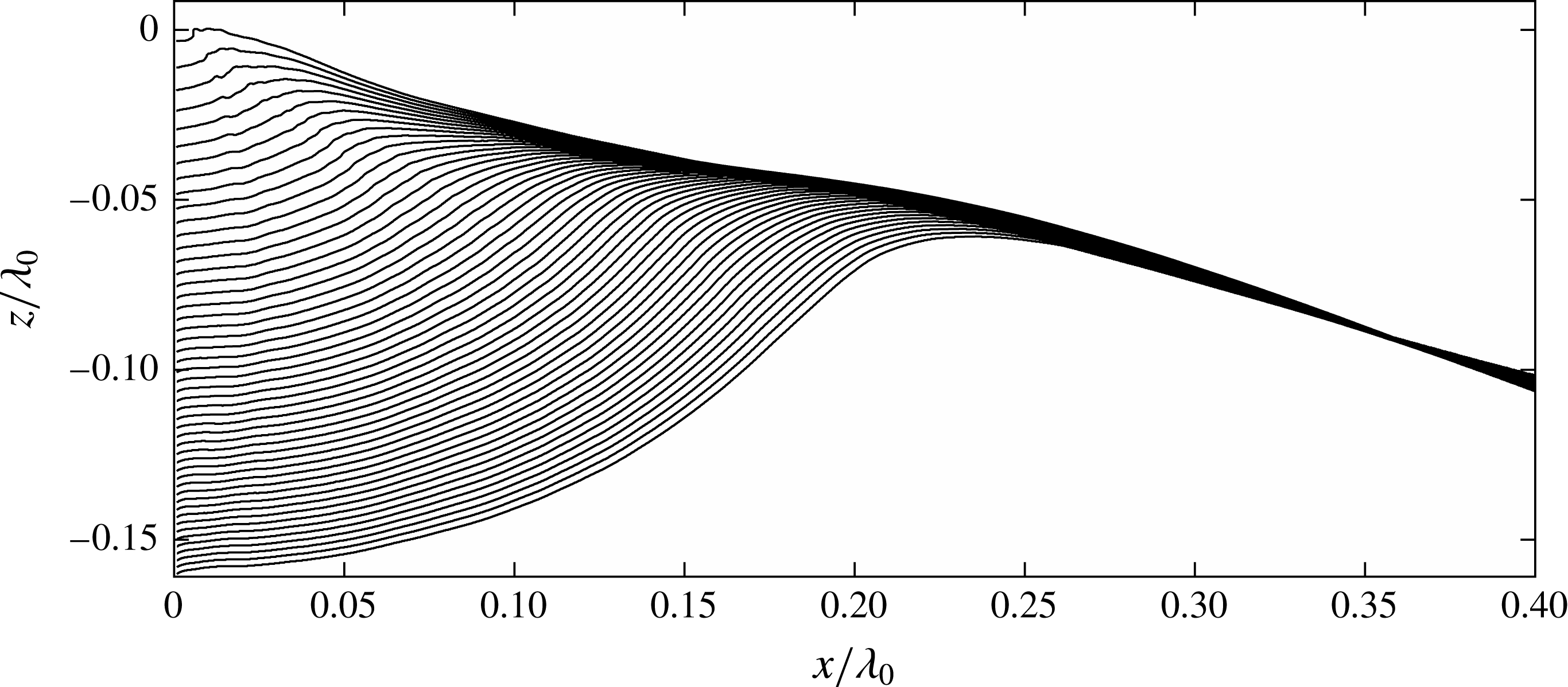
In this subsection, the focusing properties of flip-through impact will be explored in detail. Since the water surface profiles on the backsides of waves are nearly equally spaced parallel straight lines, this portion of the profiles will collapse on a single straight line in a reference frame moving at the proper constant velocity. In the present analysis, a vertical velocity is chosen for this moving reference frame in order to maintain the left edge of the profiles, i.e. the location of the front face of the structure, on a vertical line. By trial and error, it was found that the back face profiles collapsed well in a reference frame moving downward with speed of
 $0.474~\text{m}~\text{s}^{-1}=0.33\bar{c}_{p}$
and the resulting profile plot for one of the
 $z_{b}=-0.113\unicode[STIX]{x1D706}_{0}$
runs is shown in figure 17. The backside of the profiles now collapse to a thin band of lines and the main variation of the profiles during the impact is the portion between the contact point and the crest. This portion of the profiles forms a focusing surface as the crest approaches the wall.
Surface profile history for condition
 $z_{b}=-0.113\unicode[STIX]{x1D706}_{0}$
plotted in a reference frame moving vertically downward at a speed of
 $V_{r}=0.33\bar{c_{p}}$
. The time between profiles is 3.3 ms (
 $=0.0038/f_{0}$
) and the profiles are plotted from
 $tf_{0}=-0.1863$
(162 ms) to the moment of impact (
 $tf_{0}=0$
). The front face of the structure is located at
 $x/\unicode[STIX]{x1D706}_{0}=0$
. The origin of this reference frame is defined as the intersection of a line coincident with the front face of the impact structure and an extended straight line fitted to the upstream side of the wave profiles.

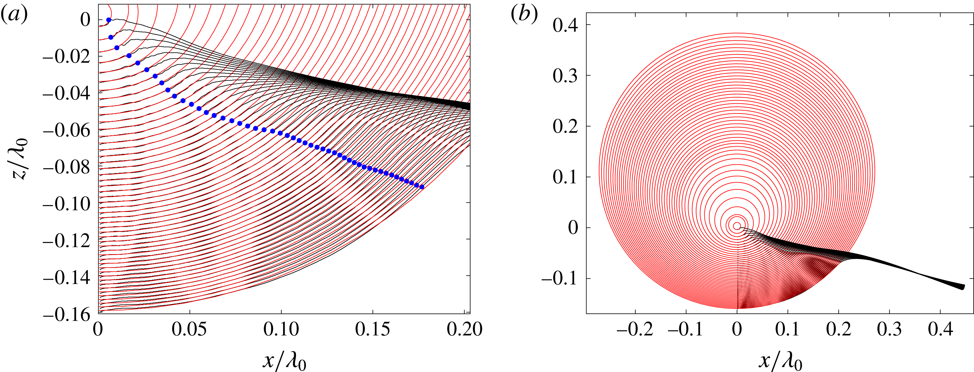
The circles fitted by the least squares method to the portion of the water surface profiles between the contact point and the inflection point downstream from the crest. The centres of the fitted circles are constrained to be on the vertical line coincident with the front face of the structure. The inflection points in the fitted curves are shown as dots in (a). The time between profiles is 3.3 ms (
 $=0.0038/f_{0}$
). (a) Close up view of the circles fitted to the profiles. (b) Expanded view of the fitted circles and the profiles.

From figure 17, it appears that the portion of the profiles forming the focusing surface are similar to circular arcs. To test this hypothesis, the upward curvature portions of the profiles adjacent to the structure were first identified numerically. This was accomplished by fitting a high-order polynomial to each surface profile and finding the location of the inflection point downstream of the crest in the fitted curves. Then, a circle constrained to have its centre on the vertical line of the front face of the structure was fitted by the least-squares method to the region of each measured profile from the water surface contact point to the
 $x$
location of the polynomial inflection point. A close up view of the profiles, fitted circles and inflection points is shown in figure 18(a) and a zoomed out view showing the profiles and the full circles is shown in figure 18(b). As can be seen in the plots, the circles fit the upward curvature portions of the profiles quite well and the radii and heights of the circle centres vary smoothly over time. From figure 18(b), it is apparent that as time progresses both the circle radius and the height of the circle centre decrease. At the moment of impact, the centre of the circle tends to
 $(x,z)=(0,0)$
, i.e. the intersection of the line forming the back face of the wave profiles and the vertical front surface of the impact structure.
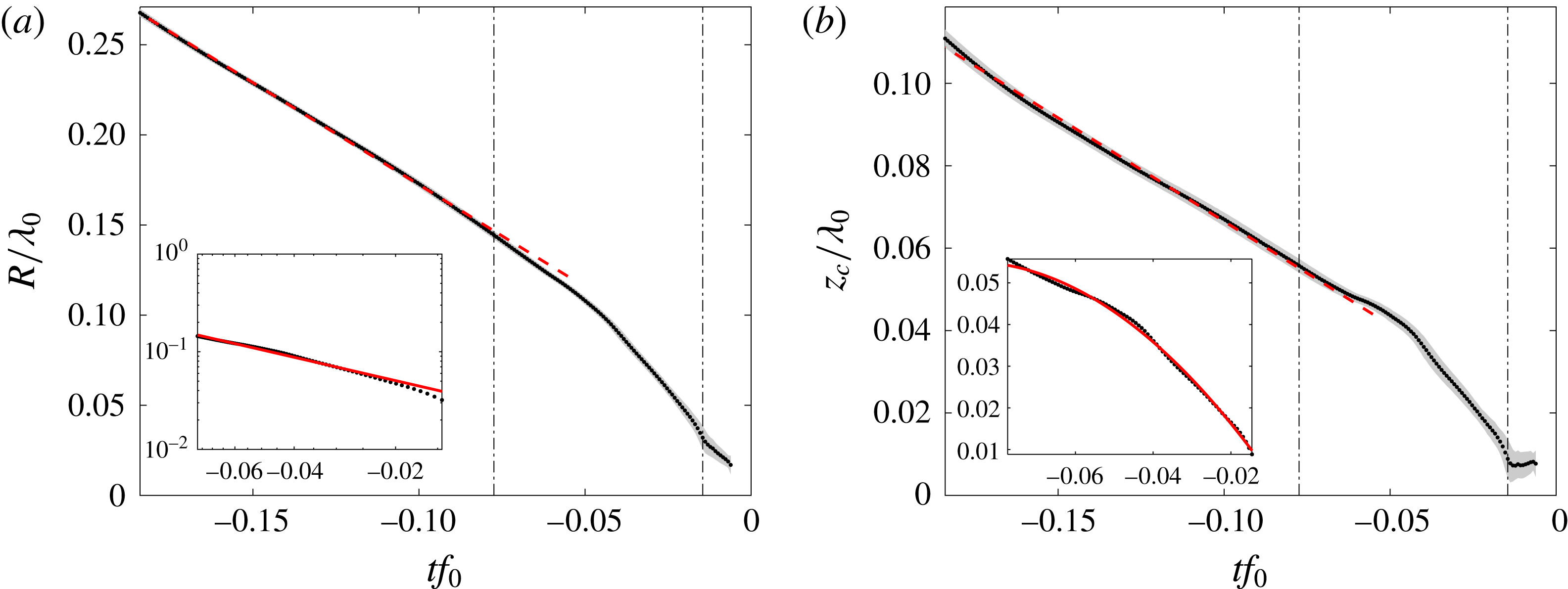
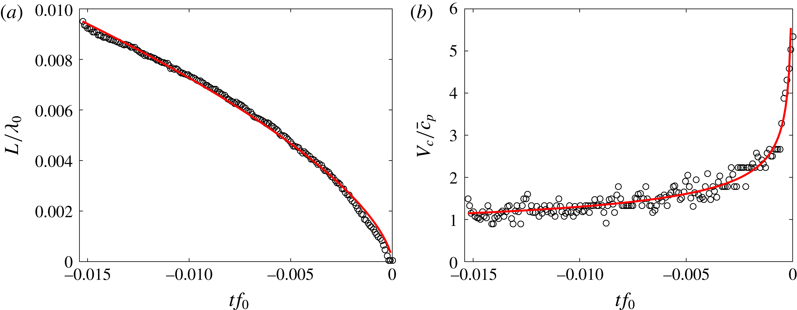
The average and standard deviation of the radius
 $R$
and centre height
 $z_{c}$
of the fitted circles from four experimental runs at
 $z_{b}/\unicode[STIX]{x1D706}_{0}=-0.113$
. The black dots are the average values of four runs and the grey band around the dots represents the uncertainty range with one standard deviation above and below the average values. The data between the two vertical lines are replotted in the inset plots with modified axes (in log–log coordinates in (a) and in linear coordinates in (b)). The values of
 $z_{c}$
are given in the moving reference frame of figure 18, the values of
 $R$
are independent of reference frame. In the insets of (a) and (b) the solid curves are the functions
 $R/\unicode[STIX]{x1D706}_{0}=1.21|tf_{0}|^{0.824}$
and
 $z_{c}/\unicode[STIX]{x1D706}_{0}=-8.65|tf_{0}|^{2}+1.52|tf_{0}|-0.01$
, respectively, which were obtained by least-squares fits to the experimental data.

A plot of the average radius (
 $R$
) and centre heights (
 $z_{c}$
) of the circles from four experimental runs with
 $z_{b}/\unicode[STIX]{x1D706}_{0}=-0.113$
are shown in 19(a) and 19(b), respectively. In this figure, data points are plotted for all frames of the high-speed movie which was recorded at 1500 f.p.s.; in figure 18, profiles for every fifth frame are plotted. As can be seen in figure 19(a),
 $R$
decreases as the time approaches
 $tf_{0}=0$
and the function
 $R(t)$
can be divided into two periods. During the first period,
 $tf_{0}<-0.077$
, the radii of the circles decrease nearly as a linear function of time. The slope of the function gives
 ${\dot{R}}=-1.54~\text{m}~\text{s}^{-1}=-1.07\bar{c_{p}}$
. In the second period,
 $-0.077<tf_{0}<-0.014$
, the radii of the circles are well approximated by a power-law function of time,
 $R/\unicode[STIX]{x1D706}_{0}\propto |tf_{0}|^{0.824}$
, the solid curve in the inset plot. When
 $-0.014<tf_{0}<0$
, the circle is not a satisfactory representation of the surface any more due to the lack of spatial resolution in this large-field-of-view data set as the surface shrinks to a very small size and due to the fact that the surface becomes rough because small-scale features on the profiles grow dramatically during this time. This late time behaviour is discussed further in § 4.2. The time evolution of
 $z_{c}$
shown in figure 19(b) is similar to the radius versus time data. As can be seen from the plot,
 $z_{c}$
moves downward following a linear function of time for the first period. In the second period, the curve resembles a parabolic function to some degree, the solid curve in the inset plot.
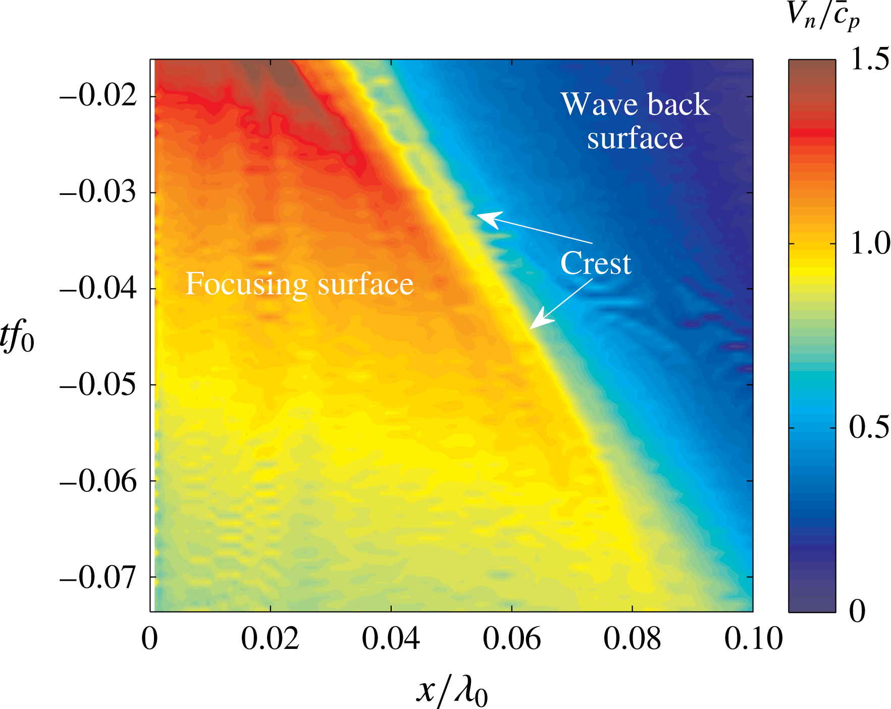
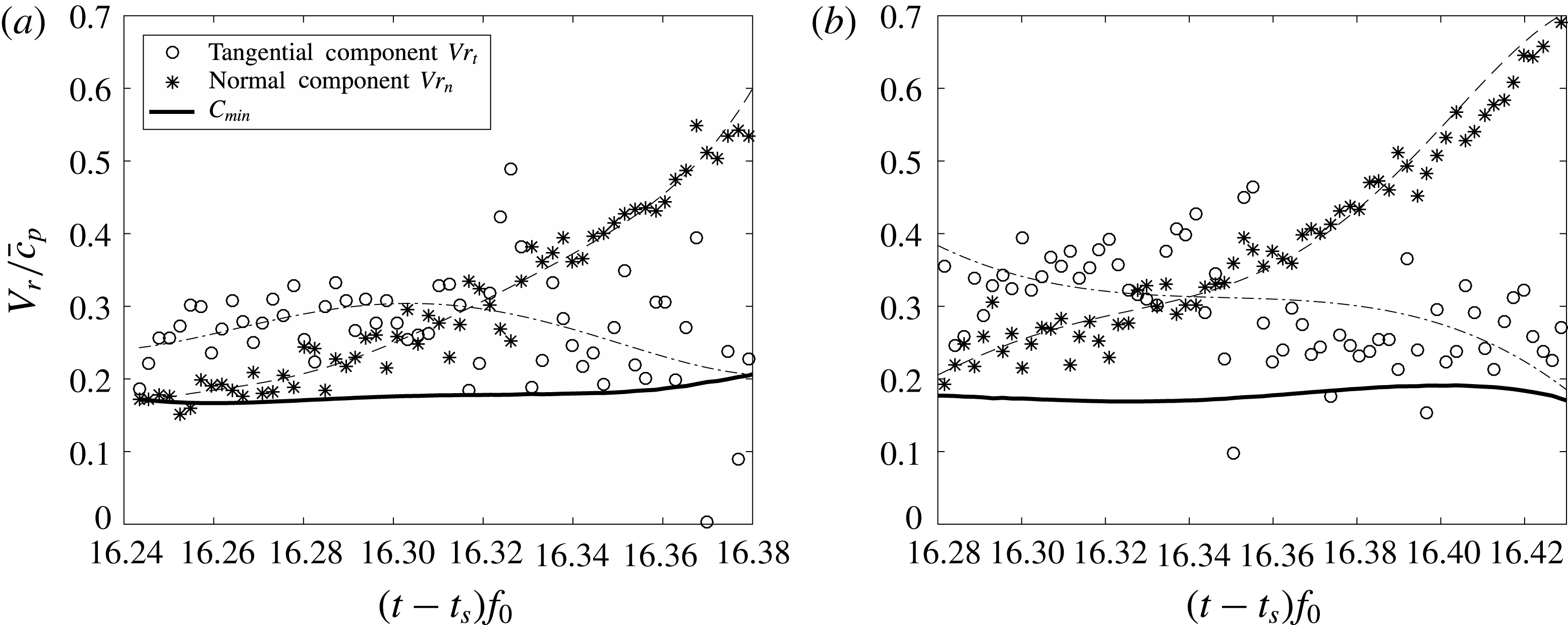
Given the motion of the centre of the circles (
 $z_{c}(t)$
), it is obvious that the normal component of the water surface velocity (
 $V_{n}$
) along the arc will not be constant as it would be if the circle centre remained fixed. Because the centre is moving downward in the moving reference frame (and in the fixed reference frame),
 $V_{n}$
increases with distance away from the wall. To demonstrate this effect,
 $V_{n}$
was calculated from the measured profiles from one experimental run by using standard smoothing and first-order difference techniques (see Wang Reference Wang2017) and a contour plot of the computed
 $V_{n}$
values on an
 $x$
–
 $t$
plane is given in figure 20. By following the magnitude of
 $V_{n}$
along any horizontal line (any fixed time) from
 $x=0$
, one can observe the increase in
 $V_{n}$
that occurs before reaching the crest.
Distribution of the normal component of surface velocity along the streamwise position over time. The calculation is performed in a reference frame moving downward at speed
 $V_{r}=0.33\bar{c_{p}}$
.

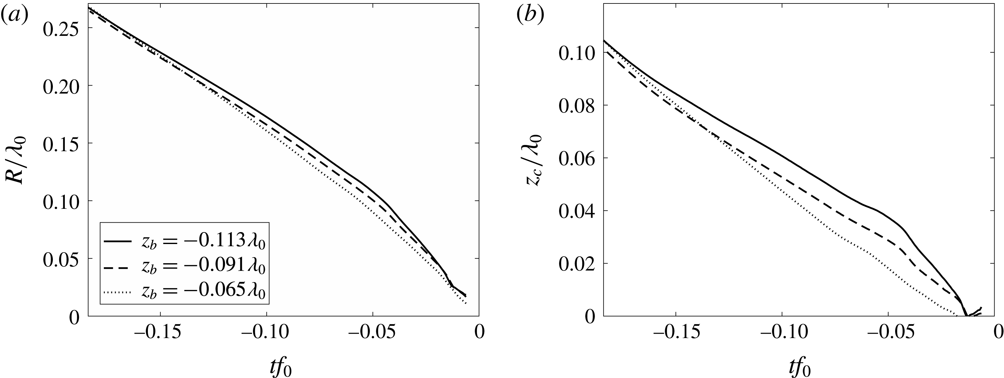
The evolution of geometrical features of the fitted circles for three values of
 $z_{b}$
. (a) Average radius of the circles versus time. (b) Average height of the circle centres (as measured in the moving reference frame of figure 18) versus time. Each curve in (a) and (b) is averaged over at least three runs. The instant when the surface profiles collapse to a point on the front face of the structure is taken as
 $tf_{0}=0$
.

The above analysis of fitting circles to the focusing surface can be applied to the remaining two flip-through experimental conditions,
 $z_{b}=-0.091\unicode[STIX]{x1D706}_{0}$
and
 $-0.065\unicode[STIX]{x1D706}_{0}$
. Plots of
 $R$
and
 $z_{c}$
versus time for all three flip-through conditions are given in 21(a) and 21(b), respectively. In all three cases,
 $z_{c}$
, is given in the moving reference frame with
 $V_{r}=-0.33\bar{c_{p}}$
, which effectively collapses the back face of the wave for all conditions because the wave speed is not significantly affected by
 $z_{b}$
. In figure 21(a), the three curves of
 $R(t)$
almost collapse, particularly at early and late times. The maximum variation between the curves occurs at approximately
 $tf_{0}=-0.05$
, where
 $\unicode[STIX]{x0394}R=0.02\unicode[STIX]{x1D706}_{0}$
. The two-function behaviour of the
 $R(t)$
curve, which was so prominent for
 $z_{b}=-0.113\unicode[STIX]{x1D706}_{0}$
, diminishes as
 $z_{b}$
increases; the data for
 $z_{b}=-0.065\unicode[STIX]{x1D706}_{0}$
are almost linear. The three curves of
 $z_{c}(t)$
in figure 21(b) all have the same qualitative shape features as the
 $R(t)$
curves, but the variation between the curves in the mid time range is more significant.
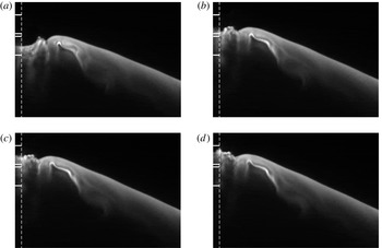
Panels (a), (b), (c), (d) are snapshots of the water surface (
 $z_{b}=-0.113\unicode[STIX]{x1D706}_{0}$
) at
 $t_{a}f_{0}=-2.2149\times 10^{-3}$
,
 $t_{b}f_{0}=-0.6820\times 10^{-3}$
,
 $t_{c}f_{0}=-0.3400\times 10^{-3}$
,
 $t_{d}f_{0}=0$
before the moment of impact, respectively. This movie is a close up view of the impact region and was taken at a frame rate of 13.5 kHz during the same experimental run as the movie corresponding to figure 5. The vertical dashed lines represent the position of the front face of the structure. The boundaries of pressure sensors 19 and 20 (centrelines at
 $z=0.0968\unicode[STIX]{x1D706}_{0}$
and
 $z=0.1022\unicode[STIX]{x1D706}_{0}$
, respectively) are shown as horizontal solid white lines; the first and second lines from the bottom are the boundaries of sensor 19 and the third and fourth lines are the boundaries of sensor 20. The field of view of these images is
 $4.8~\text{cm}\times 4.3~\text{cm}$
. The movie from which these images were taken is available as supplementary material, filename: Movie 6.mp4.

4.2 Characteristics of the impact pressure and its related properties
This section is broken into six subsections in which the analysis of the pressure measurements, the theory, the acceleration of the contact point and the importance of surface tension in class I (flip-through) impacts are discussed in §§ 4.2.1–4.2.4, respectively, the pressure oscillations in class II impacts are discussed in § 4.2.5 and the pressure pulse during class III impact is discussed in § 4.2.6.
4.2.1 Class I (flip-through) impact – analysis of pressure measurements
In the flip-through cases, the impact pressure on the wall is found to be very sensitive to the detailed geometry of the water surface just before the moment of impact, as is demonstrated below. Here we consider the
 $z_{b}=-0.113\unicode[STIX]{x1D706}_{0}$
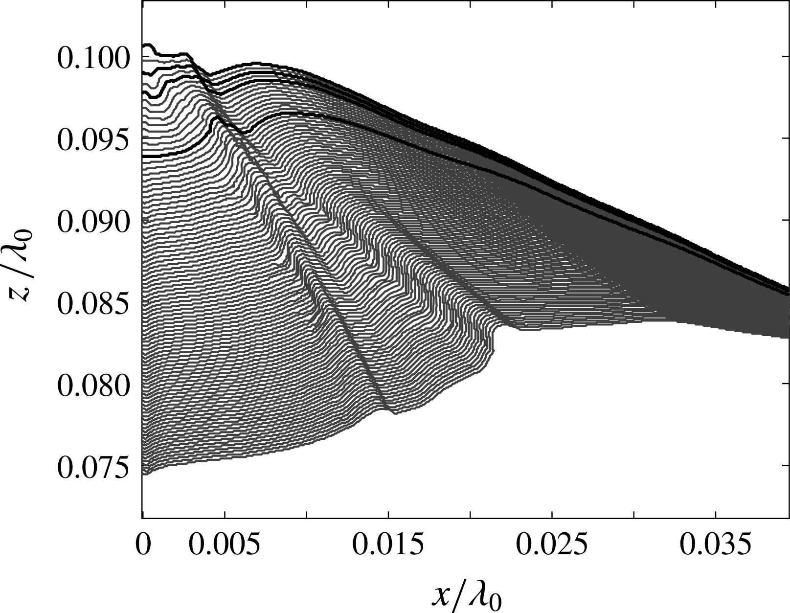
case, which has been discussed above using photographs from a high-speed movie in figure 5 and the corresponding water surface profile history and pressure contour plots in figures 6(a) and 16(a), respectively. In figure 16(a), a double pressure peak is found. In order to understand the double peak phenomenon, LIF movies with higher temporal resolution and zoomed in at the zone of impact were taken. Four images from one of these movies are shown in figure 22. The surface profiles from the movie and the pressure measurements are shown in figures 23 and 24, respectively. The instants when the images in 22(a), 22(b), 22(c) and 22(d) are taken are called
 $t_{a}$
,
 $t_{b}$
,
 $t_{c}$
and
 $t_{d}$
, respectively, and are defined in the caption of figure 22 and marked on the plots in figure 24(a,b), see figure captions for additional details.
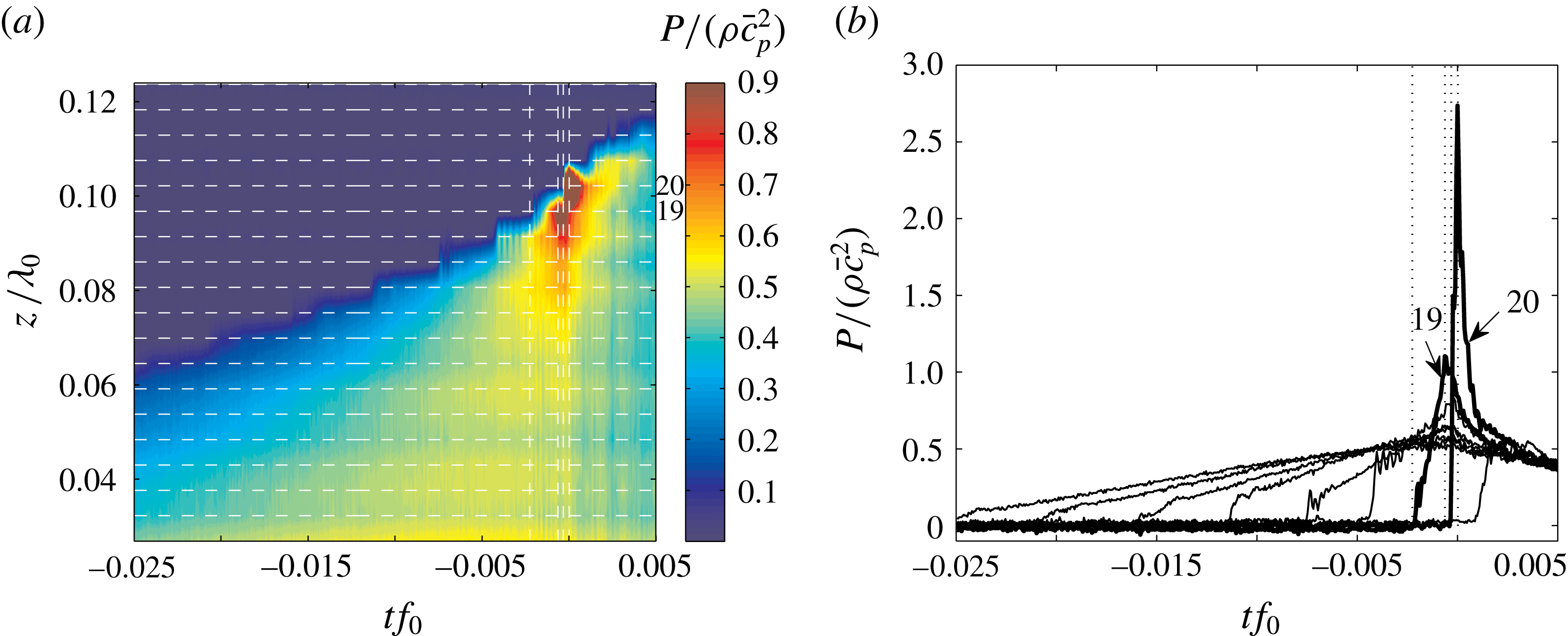
The double pressure peak can be seen clearly in figure 24(b). The magnitudes of the two pressure peaks are significantly larger than the pressures measured at the other heights over all time. The earlier peak and later peak were measured by two adjacent pressure sensors, 19 and 20, respectively. The time
 $t_{a}$
is the instant when the earlier pressure peak starts to rise from zero, according to figure 24(b). Figure 22(a) shows that at
 $t=t_{a}$
, the contact point has climbed slightly above the lower boundary of sensor 19. At
 $t=t_{b}$
, the earlier peak reaches its maximum value, see figure 24(b). As shown in figure 22(b), at
 $t=t_{b}$
, the contact point almost reaches the upper boundary of the sensor 19. At this instant, the tip of a small jet formed at the crest, see figure 22(b), is still upstream of the wall. This indicates there has not yet been direct impact of the jet with the wall. Therefore, the earlier pressure peak is probably caused by the focusing of the surface. The later peak has a higher maximum than the earlier peak and is measured by pressure sensor 20. As shown in figure 22(c), at
 $t=t_{c}$
, when the later peak starts to rise, the small jet on the surface just impinges on pressure sensor 20. This indicates that the later peak (with the highest magnitude) might be caused by the direct impact of a small jet on the wall. The later peak reaches its maximum at
 $t=t_{d}$
when the small jet has already impinged on the wall, see figure 22(d). These synchronized images and pressure records provide strong evidence that the earlier pressure peak on the wall is a unique feature of flip-through impact, as described in some previous theoretical work, and the higher second peak is likely to have been strongly influenced by the impact of the jet. However, the finite size and slight separation of the two pressure sensors, indicates that pressure measurements with improved spatial resolution would be needed to prove this hypothesis.
Surface profiles near the impact zone before the moment of impact for condition
 $z_{b}=-0.113\unicode[STIX]{x1D706}_{0}$
. These profiles were obtained from the movie corresponding to figure 22. The profiles are from every other movie frame and the time interval between adjacent profiles is 0.149 ms (
 $=0.000171/f_{0}$
). The total time range for these profiles is 13.33 ms (
 $=0.01533/f_{0}$
). The profiles shown in bold correspond to the images shown in figure 22(a–d).

A contour plot for the pressure evolution on the wall at
 $z_{b}=-0.113\unicode[STIX]{x1D706}_{0}$
is shown in (a). This is a zoomed in view of the region of maximum pressure from figure 16(a). The horizontal lines represent the centrelines of the pressure sensors; the sensor number increases monotonically with
 $z$
and sensors 19 and 20 are marked on the figure. The time histories of the pressures measured by sensors 14 to 20 are shown in (b); the highest pressure is measured by sensor 20. The four vertical white lines in (a) and grey dotted lines in (b) from left to right represent the times corresponding to the images shown in 22(a), 22(b), 22(c) and 22(d), respectively.

4.2.2 Class I (flip-through) impact – theoretical analysis
With existing theory, it is possible to understand better the physics that creates these temporally and spatially localized high-pressure regions during flip-through impact. Since the time scale of the flip-through impact is short, viscous effects from the wall cannot affect the outer flow and the phenomenon can be well described by potential flow theory. According to Bernoulli’s equation, the pressure on the wall consists of two parts: the dynamic pressure (defined herein as the sum of the unsteady term
 $\unicode[STIX]{x1D70C}\unicode[STIX]{x2202}\unicode[STIX]{x1D719}/\unicode[STIX]{x2202}t$
and the nonlinear term
 $0.5\unicode[STIX]{x1D70C}(\unicode[STIX]{x1D735}\unicode[STIX]{x1D719})^{2}$
) and the hydrostatic pressure (
 $\unicode[STIX]{x1D70C}gz$
). The potential flow model proposed by Cooker (Reference Cooker2002) describes several types of focusing flows with indented free surfaces, similar to that found in the present experiments. In one of the calculations presented in the paper, at any instant in time, the water surface consists of an horizontal portion and a semi-circular indentation with radius
 $R$
. It is assumed the flow field is described by a line sink placed at the centre of the semi-circle. The instantaneous normal velocity of any point on the circular arc is
 $V$
and the normal velocity on the surrounding flat free surface is zero. Given
 $R$
and
 $V$
at any instant in time, the theory predicts the pressure field in the fluid domain
 $r\geqslant R$
as
 $$\begin{eqnarray}\displaystyle \displaystyle \frac{p(r,\unicode[STIX]{x1D703})}{\unicode[STIX]{x1D70C}V^{2}} & = & \displaystyle \frac{1}{Fr^{2}}\cos \unicode[STIX]{x1D703}\left(\frac{r}{R}\right)+\left(\frac{8}{3\unicode[STIX]{x03C0}}-\frac{1}{Fr^{2}}\right)\cos \unicode[STIX]{x1D703}\left(\frac{R}{r}\right)\nonumber\\ \displaystyle & & \displaystyle -\,\frac{1}{2}(1+\cos 2\unicode[STIX]{x1D703})\left(\frac{R}{r}\right)^{2}-\frac{1}{2}\mathop{\sum }_{n=2}^{\infty }a_{n}\cos [2n-1]\unicode[STIX]{x1D703}\left(\frac{R}{r}\right)^{2n-1},\end{eqnarray}$$
where the plane polar angle
 $\unicode[STIX]{x1D703}$
is measured from the vertically downward direction and
 $$\begin{eqnarray}\displaystyle & \displaystyle a_{n}=\frac{16}{\unicode[STIX]{x03C0}}\frac{(-1)^{n+1}}{(4n^{2}-1)(2n-3)}, & \displaystyle\end{eqnarray}$$
and
 $Fr$
is the Froude number defined as
 $Fr=V/\sqrt{gR}$
. On the line of symmetry at
 $\unicode[STIX]{x1D703}=0^{\circ }$
(the front face of the structure in the present experiments), equation (4.1) reduces to
 $$\begin{eqnarray}\displaystyle & \displaystyle \frac{p_{w}(r)}{\unicode[STIX]{x1D70C}V^{2}}=\frac{1}{Fr^{2}}\left(\frac{r}{R}\right)+\left(\frac{8}{3\unicode[STIX]{x03C0}}-\frac{1}{Fr^{2}}\right)\left(\frac{R}{r}\right)-\left(\frac{R}{r}\right)^{2}-\frac{1}{2}\mathop{\sum }_{n=2}^{\infty }a_{n}\left(\frac{R}{r}\right)^{2n-1}. & \displaystyle\end{eqnarray}$$
The first term in (4.1) (and (4.3)) is multiplied by
 $1/Fr^{2}$
. This term is the hydrostatic pressure, which, of course, produces horizontal contours of constant pressure that increase linearly with depth. Only one other term in (4.1) and (4.3) is influenced by gravity, i.e. is multiplied by
 $1/Fr^{2}$
. This second term is part of the effect of unsteadiness, as explained in Cooker (Reference Cooker2002), and produces a pressure field that is negative in the domain of the fluid and decreases in magnitude monotonically with increasing
 $r/R$
at fixed
 $\unicode[STIX]{x1D703}$
. Herein, the combined contribution from these two terms is called the gravitational effect, and it is found numerically that this part of the pressure increases monotonically with increasing depth at any horizontal position. The pressure from the combined effect of the remaining terms (those independent of
 $Fr$
) is herein called the inertial effect and is plotted in figure 2 in Cooker (Reference Cooker2002). These contours of dimensionless pressure are only a function of
 $R/r$
and
 $\unicode[STIX]{x1D703}$
and include a subsurface pressure maximum. Thus, whether or not a subsurface maximum exists in the total pressure field depends on the instantaneous value of
 $Fr$
since it controls the relative magnitude of the gravitational and inertial pressure fields. In the unsteady situation of the flip-through wave impact of the present experiments, the instantaneous value of
 $Fr$
increases continuously with time, as will be demonstrated below. As the impact begins,
 $Fr$
is small and the gravitational effect dominates. As a result, equation (4.1) indicates that no pressure maximum exists below the free surface, as shown in figure 25(a) (
 $Fr=5.78$
). After
 $Fr$
reaches a critical value (
 $Fr_{m}\approx 7$
as predicted by (4.3)), the inertial effect becomes dominant and a localized maximum pressure appears, as is shown in figure 25(b) (
 $Fr=9.80$
). Thus, prediction of the time when the critical Froude number is reached and the subsurface pressure maximum occurs in the experiment requires the function
 $Fr(t)$
. The determination of this function from the experimental data is addressed in the following.
Pressure distributions in the flow field computed by (4.1) at
 $Fr=5.78$
and
 $Fr=9.80$
are shown in (a) and (b), respectively. Temporal evolution of the pressure distribution on the wall computed from (4.3) is shown in (c). The two vertical dashed lines on the left and right in (c) represent the times corresponding to the pressure fields in (a) and (b), respectively. In this calculation, the required temporal variation of the contact point height and Froude number is taken from the experimental data, see text for details.

Though Cooker’s model is not directly applicable to the present experiments, it can be used to gain some insight into the flow dynamics. The difference between the two flows includes the boundary shape outside the circular arc and the distribution of normal velocity along the circular arc. Thus, in order to apply the model to the experiments, we need to make some choices forced by the differences in the surface shapes and motions. An alternative choice for the radius in the experiments is the length scale
 $L(t)$
defined as the height difference between the contact point and the crest. Since the averaged surface normal velocity on the circular arc is difficult to obtain, particularly when the surface shrinks to a small size, the contact point velocity
 $V_{cp}$
will be chosen as the velocity scale. Plots of
 $L$
and
 $V_{cp}$
versus time are given in figure 26 for one experimental run at
 $z_{b}=-0.113\unicode[STIX]{x1D706}_{0}$
. The solid curve in each plot is a least-squares fit of a power-law function to the data, see figure caption for equations.
The temporal evolution of length scale
 $L$
and velocity scale
 $V_{cp}$
from the experiment are shown in (a) and (b), respectively. See text for the definition of
 $L$
and
 $V_{cp}$
. In (b), the circles are the velocity values computed from finite difference of the contact point position versus time data from the experiments. The solid curves in (a) and (b) are power-law functions that were obtained by least-squares fits to the experimental data: (a)
 $L/\unicode[STIX]{x1D706}_{0}=0.1366|tf_{0}|^{0.637}$
and (b)
 $V_{cp}/\bar{c_{p}}=0.3214|tf_{0}|^{-0.304}$
. The proximity of the exponents
 $0.637$
and
 $-0.304$
to
 $2/3$
and
 $-1/3$
, respectively, is discussed in § 4.2.4.

Using the data from figure 26, the evolution of
 $Fr$
versus time before the moment of impact is calculated and plotted in figure 27(a). The spread of data points mostly comes from the numerical error when taking derivatives of the contact point position to obtain
 $V_{cp}(t)$
. Starting from
 $tf_{0}=-0.015$
,
 $Fr$
gradually increases following a nearly linear curve. After approximately
 $tf_{0}=-0.008$
,
 $Fr$
increases rapidly over time. From the pressure record shown in figure 24, when
 $tf_{0}>-0.00225$
(shown by the first dash vertical line), the pressure measured by the sensor just below the free surface is larger than the pressures measured by all the lower sensors. This indicates the pressure maximum starts to occur after this instant. In figure 27(a), this time is labelled as
 $t_{e}f_{0}$
and the corresponding value of
 $Fr$
is
 $Fr_{e}\approx 15$
. At later times,
 $Fr$
exceeds
 $Fr_{e}$
and a pressure maximum always occurs below the contact point.
Cooker’s theory can also be used to create a theoretical/experimental pressure contour plot for direct comparison with the plot in figure 24(a). In addition to
 $Fr(t)$
and
 $L(t)$
, the calculation requires the contact point height data,
 $z_{cp}(t)$
, which was also used to determine
 $L(t)$
. The resulting pressure contour plot is given in figure 25(c). This prediction is qualitatively similar to the experimentally measured data shown in the other figure; however, the spatially localized pressure maximum, appears after approximately
 $tf_{0}=-0.0088$
, corresponding to
 $Fr\approx 7$
. Given the differences between the flows in experiments and theory, the mismatch of the critical Froude numbers and times is to be expected. However, both the experimental results and Cooker’s model strongly support the idea that the instantaneous
 $Fr$
determines whether a pressure maximum exists below the free surface.
Froude number (
 $Fr$
) and Weber number (
 $We$
) versus time from experiments are presented in (a) and (b), respectively. The length scale and velocity scale used to compute
 $Fr$
and
 $We$
are taken from the data shown in figure 26. The vertical lines in (a) and (b) represent the time when the local pressure maximum starts to occur in the experiments. The inset of (a) is the close up view of the main plot. The solid curve in (a) is the function
 $Fr(t)=0.367|tf_{0}|^{-0.623}$
, obtained from the power-law fitting of
 $L(t)$
and
 $V_{cp}(t)$
shown in figure 26.

Similar features of the impact pressure in the flip-through condition are also reported in Bredmose et al. (Reference Bredmose, Peregrine and Bullock2009). In this work, numerical simulations of a shallow-water wave impact on a wall that extends to the bottom of the tank are performed. In the flip-through condition, their results (figure 12 in the paper) show an isolated pressure maximum on the wall approximately 10 ms (
 $=0.0115/f_{0}$
) before the impact, analogous to the present experiments. At early times before impact, the pressure on the wall increases with depth. The pressure peak only lasts for approximately 15 ms (
 $=0.0173/f_{0}$
).
4.2.3 Class I (flip-through) impact – the vertical jet
The acceleration of the high-speed vertical jet has received considerable attention in the literature, see for example Cooker & Peregrine (Reference Cooker, Peregrine, Banner and Grimshaw1992). Previous studies have shown that this high acceleration is caused by the high pressure gradient between the location of the maximum pressure and the free surface. However, it is difficult to measure the acceleration of the flow directly. Instead, the acceleration of the flow near the contact point can be estimated by twice differentiating the contact point position versus time data (measured at a frame rate of 13.5 kHz). To avoid the noise created by a second-order finite difference method on the position versus time data, a third-order polynomial fitting function is applied to the contact point position versus time data and the acceleration of the contact point is estimated from the second-order derivative of this fitting function. Using this method, it is found that the estimated acceleration of the contact point can reach as high as
 $481g$
in the present experiments. Due to the limitations of the temporal resolution and the accuracy of the curve fitting, the exact value of the maximum contact point acceleration is still difficult to obtain. Nevertheless, the high estimated value provides additional evidence of the existence of a subsurface region with a high pressure gradient.
4.2.4 Class I (flip-through) impact – surface tension
As the moment of impact is approached, the growth of the small-scale features on the water surface profile (see the profile history in figure 23) may indicate that surface tension begins to play an important role. To explore this possibility, the Weber number at each time,
 $$\begin{eqnarray}\displaystyle & \displaystyle We(t)=\frac{\unicode[STIX]{x1D70C}V_{cp}(t)^{2}L(t)}{\unicode[STIX]{x1D70E}}, & \displaystyle\end{eqnarray}$$
was calculated from the length and velocity scales plotted in figure 26 and the result,
 $We$
versus
 $t$
, is plotted in figure 27(b). The values of
 $We$
are spread around a constant level approximately
 $We=400$
for most of the impact process, indicating that inertia effects dominate surface tension. This is consistent with power-law scaling functions proportional to
 $t^{1/3}$
and
 $t^{-2/3}$
for
 $V_{cp}$
and
 $L$
, respectively, see the caption to figure 26 and the discussion in, for example, Longuet-Higgins (Reference Longuet-Higgins1993). Near the moment of impact,
 $-0.0025<tf_{0}<0$
,
 $We$
decreases from the constant level to nearly zero. This latter behaviour is consistent with
 $V_{cp}$
tending to a finite value and
 $L$
tending to zero as
 $t$
tends to
 $0$
. Using the power-law functions for
 $L(t)$
and
 $V_{cp}(t)$
as given in the caption of figure 26, or the corresponding rational values of
 $2/3$
and
 $-1/3$
, to represent
 $L(t)$
and
 $V_{cp}(t)$
in the calculation of
 $We(t)$
does not produce the final stage of the data in figure 27(b) because the power laws do not fit the
 $L$
-
 $V_{cp}$
data well at small times. In particular, the
 $V_{cp}(t)$
power law tends to
 $\infty$
as
 $t$
tends to zero, rather than a maximum value as observed in the experiments. This late time inconsistency between the power-law functions and the data is as expected for a real physical system and may indicate an ultraviolet cutoff of the divergent process, as is also described in Zeff et al. (Reference Zeff, Kleber, Fineberg and Lathrop2000).
4.2.5 Class II impact – pressure oscillations
One of the very prominent features of the pressure contour plot at
 $z_{b}=0.0$
, shown in figure 16(b), is the pressure oscillation that occurs nearly in phase over the vertical row of sensors. Images in figure 9 indicate that, during the impact process, a crater exists between the front face of the structure and the growing jet that issues from the crest. When the jet meets the rising water column, it is possible that part of the air within the crater cannot escape. Therefore, it is very likely that the pressure oscillation is caused by the entrainment of air bubbles. Unfortunately, the LIF movies and other visualizations that have been attempted are not able to see into this flow region to observe the bubbles. However, bubble oscillation theory will be used here to compute the diameter of a spherical bubble with the oscillation frequency measured in the experiments. The natural frequency of a spherical bubble in water can be estimated by (Plesset & Prosperetti Reference Plesset and Prosperetti1977)
 $$\begin{eqnarray}\displaystyle & \displaystyle f_{n}=\frac{1}{2\unicode[STIX]{x03C0}R_{0}}\sqrt{\frac{3kP_{eq}}{\unicode[STIX]{x1D70C}}-\frac{2\unicode[STIX]{x1D70E}}{\unicode[STIX]{x1D70C}R_{0}}}, & \displaystyle\end{eqnarray}$$
where
 $R_{0}$
is the radius of the bubble at equilibrium state,
 $\unicode[STIX]{x1D70C}$
is the density of water,
 $k=1.4$
is the heat capacity ratio of air,
 $\unicode[STIX]{x1D70E}=73~\text{mN}~\text{m}^{-1}$
is the surface tension of water,
 $P_{eq}$
is the pressure inside the bubble at equilibrium state and
 $$\begin{eqnarray}\displaystyle & \displaystyle P_{eq}=P_{\infty }+\frac{2\unicode[STIX]{x1D70E}}{R_{0}}. & \displaystyle\end{eqnarray}$$
According to (4.5), the 1000 Hz pressure oscillation frequency corresponds to the natural frequency of a spherical air bubble with a radius of 3.28 mm under ambient pressure of 1 atm. At a later time, oscillations with higher frequencies (2800 Hz) are observed, corresponding to bubbles with radius as small as 1.17 mm. The low-frequency component of the oscillation at 1000 Hz covers a wide range of heights below the free surface with very little phase shift with increasing depth. This indicates that the acoustic waves that are most likely generated near the free surface transmit through the fluid at very high speed. In the computational work by Bredmose et al. (Reference Bredmose, Peregrine and Bullock2009, Reference Bredmose, Bullock and Hogg2015), in the case of air entrainment, similar pressure oscillations are found. In their simulation, in cases when the fluid has non-zero initial aeration level, the propagation speed of the acoustic waves is decreased, causing a more noticeable phase shift in the pressure oscillation with increasing depth.
4.2.6 Class III impact – analysis of pressure measurements
In the two cases of class III impact, two prominent differences are observed between the two conditions. First, the impact pressure measured at
 $z_{b}=0.043\unicode[STIX]{x1D706}_{0}$
is much higher than that measured at
 $z_{b}=0.022\unicode[STIX]{x1D706}_{0}$
. Comparison of the images in figures 13 and 14 shows that the rising water column along the wall at
 $z_{b}=0.043\unicode[STIX]{x1D706}_{0}$
is thinner than that at
 $z_{b}=0.022\unicode[STIX]{x1D706}_{0}$
. This difference may be caused by the smaller time available for the water column to develop before the plunging jet arrives in the
 $z_{b}=0.043\unicode[STIX]{x1D706}_{0}$
case. Perhaps then, for
 $z_{b}=0.043\unicode[STIX]{x1D706}_{0}$
, the horizontal momentum carried by the plunging jet is less attenuated by the water column during impact, causing the higher pressure at this condition. Second, a pressure oscillation occurs at
 $z_{b}=0.043\unicode[STIX]{x1D706}_{0}$
and not at
 $z_{b}=0.022\unicode[STIX]{x1D706}_{0}$
. This difference is likely to be associated with the differences in the detailed geometry of the water surface (see figures 13 and 14) after it first touches the bottom of the structure. It is hypothesized that air is entrained at
 $z_{b}=0.043\unicode[STIX]{x1D706}_{0}$
as a result of the collision between the plunging jet and a micro-jet (see figure 14
e), which is generated at the bottom corner of the structure at the initial impact. At the initial impact for the
 $z_{b}=0.022\unicode[STIX]{x1D706}_{0}$
case, a ripple is formed instead. This growing ripple eventually merges with the plunging jet in a smooth process without direct collision. The fluid momentum near the bottom corner of the structure at initial impact is probably relevant to these detailed responses of the water surface. To further examine this possibility, the temporal evolution of the vertical velocity (
 $V_{s}$
) of the water surface of the undisturbed breaker at the streamwise tank position of the vertical wall,
 $x=0$
, is shown in figure 28. The instants when the water surface at
 $x=0$
reaches the bottom corner of the structure (initial impact) for these two conditions are shown in the figure. The vertical velocity of the water surface at
 $x=0$
is
 $V_{s}=0.28\bar{c_{p}}$
at
 $z_{b}=0.022\unicode[STIX]{x1D706}_{0}$
and
 $V_{s}=0.73\bar{c_{p}}$
at
 $z_{b}=0.043\unicode[STIX]{x1D706}_{0}$
. The larger
 $V_{s}$
indicates the water surface impacts the bottom of the structure with more momentum. This may contribute to the formation of the micro-jet in the case
 $z_{b}=0.043\unicode[STIX]{x1D706}_{0}$
and subsequent air entrainment. However, at
 $z_{b}=0.022\unicode[STIX]{x1D706}_{0}$
, with less fluid momentum, a ripple instead of a micro-jet is generated and no air seems to be entrained. There possibly exists a boundary for the value of
 $z_{b}$
between the two conditions for the pressure oscillations to occur.
Vertical velocity at the surface of the undisturbed breaker at the same streamwise position (
 $x=0$
) as the front surface of the structure versus time. The time
 $t_{s}$
is the instant when the wave maker starts moving. The vertical line on the left (dotted) represents the time (
 $(t-t_{s})f_{0}=16.39$
) when the breaker surface touches the lower front corner of the wall at condition
 $z_{b}/\unicode[STIX]{x1D706}_{0}=0.022$
. The vertical line on the right (dash-dot) represents the time (
 $(t-t_{s})f_{0}=16.46$
) when the breaker surface touches the lower front corner of the wall at condition
 $z_{b}/\unicode[STIX]{x1D706}_{0}=0.043$
. The bold dashed line is the polynomial fit to the velocity data. The values of
 $W_{0}$
at the above two times are found by interpolation of this polynomial.

4.3 Upstream-propagating waves
Analysis of water surface profile histories like those shown in figures 6(a) and 10 indicate that the interaction of the wave packet with the wall creates three types of upstream propagating waves. To understand these upstream-propagating waves, it is important to recognize that there are a number of small-amplitude wave crests that reach the wall prior to the large crest whose behaviour has been the main focus of the discussion so far. These small-amplitude waves are the result of imperfections in the wave packet focusing process and can be seen clearly in the plot of water surface height at
 $x=0$
versus time for the
 $z_{b}\leqslant 0$
and open-water cases as shown in figure 29. The first type of upstream-propagating waves considered here are caused by reflection of the small-amplitude waves discussed above. These reflections have the same frequencies as the incoming waves and might be responsible for the undular shape of the upper edge of the envelope of the water surface profiles shown in figure 6(a) (
 $z_{b}=-0.113\unicode[STIX]{x1D706}_{0}$
) as compared to the flat shape of the envelope in the open-water case, see figure 6(b). In the case of a perfect reflection of an infinite uniform linear wavetrain with amplitude
 $a$
and wavelength
 $\unicode[STIX]{x1D706}$
, the envelope would look like a rectified sinusoid and have a maximum at the wall with amplitude
 $2a$
and the first node at
 $x=\unicode[STIX]{x1D706}_{0}/4$
. In the present case, the reflection is imperfect due to the finite submergence of the bottom of the structure, the non-uniformity of the wavetrain and, probably, nonlinear wave effects. In the profile history shown in figure 6(a), there is a global maximum of the envelope height at the wall, a local minimum at
 $x\approx 0.09\unicode[STIX]{x1D706}_{0}$
and a local maximum at
 $x\approx 0.25\unicode[STIX]{x1D706}_{0}$
. As the submergence is increased, the peak-to-trough height of the wave profile envelope increases (see figure 8) and the water surface height at
 $x=0$
oscillates with a larger amplitude during impact (see figure 29), indicating that the reflection is stronger.
The surface height at
 $x=0$
versus time with the structure installed at different
 $z_{b}$
and for the breaker in open water. Each line is the average over three experimental runs. The mean water level is
 $z=0$
. The inset plot is an expanded view of the period between the two vertical dashed lines in the main plot.

Water surface profile histories for cases
 $z_{b}=-0.113\unicode[STIX]{x1D706}_{0}$
,
 $z_{b}=-0.065\unicode[STIX]{x1D706}_{0}$
and
 $z_{b}=0.0$
are given in panels (a), (b) and (c), respectively, and profiles from a sine wave simulation are given in panel (d). The profiles are plotted in a reference frame moving horizontally with the speed of the crest point of the breaker in open water,
 $u_{c}=1.5~\text{m}~\text{s}^{-1}$
. The sine wave simulation consists of a left moving gravity wave with amplitude
 $a_{\ell }=0.11~\text{m}$
and wavelength
 $\unicode[STIX]{x1D706}_{\ell }=1.44~\text{m}$
(
 $u_{c}=1.5~\text{m}~\text{s}^{-1}$
) and a right moving wave with
 $a_{r}=0.005~\text{m}$
and
 $\unicode[STIX]{x1D706}_{r}=0.24~\text{m}$
. In all cases, the
 $i\text{th}$
profile is shifted upward by
 $(i-1)\,\text{d}z~\text{cm}$
, where
 $\text{d}z=0.6~\text{cm}$
. The time interval between consecutive profiles is 3.3 ms (
 $=0.0038/f_{0}$
). The bold solid lines are the trajectories of the crest points.

A second type of upstream-propagating wave can be detected by mapping the trajectory of the crest point (defined as the point of maximum height of the wave profile) during the impact. To this end, water surface profile histories for
 $z_{b}=-0.113\unicode[STIX]{x1D706}_{0}$
,
 $z_{b}=-0.065\unicode[STIX]{x1D706}_{0}$
,
 $z_{b}=0$
are shown in 30(a), 30(b) and 30(c), respectively. The profile histories are shown in a reference frame moving to the left with the speed of the wave crest in open water,
 $u_{c}=1.044\overline{c}_{p}=1.5~\text{m}~\text{s}^{-1}$
. As can be seen from the plots, the crest point trajectory has a zig–zag shape in which periods of relatively slow upstream (to the right) motion are periodically interrupted by sudden downstream motion. This behaviour becomes more pronounced as
 $z_{b}$
decreases. It is hypothesized that the zig–zag trajectories are due to a high-frequency upstream-propagating wave component. In order to explore this hypothesis, a simple simulation consisting of the addition of left- and right-propagating linear gravity waves was performed. The left-propagating wave, representing the incoming wave in the experiment, has a phase speed equal to
 $u_{c}$
(wavelength
 $\unicode[STIX]{x1D706}_{\ell }=1.44~\text{m}$
) and amplitude
 $a_{\ell }=0.11~\text{m}$
. The right-propagating wave, representing a wave reflected by or generated at the structure, has a wavelength
 $\unicode[STIX]{x1D706}_{r}<\unicode[STIX]{x1D706}_{\ell }$
and an amplitude
 $a_{r}<a_{\ell }$
. The profile histories and crest point trajectories from this model are presented in plot (d) in the same reference frame and coordinates as was the experimental data;
 $a_{r}$
and
 $\unicode[STIX]{x1D706}_{r}$
were adjusted to make the crest point trajectory match that for the
 $z_{b}=0.0$
case, resulting in the values
 $a_{r}=0.005~\text{m}$
and
 $\unicode[STIX]{x1D706}_{r}=\unicode[STIX]{x1D706}_{\ell }/6$
. The wave period corresponding to this
 $\unicode[STIX]{x1D706}_{r}$
is 0.39 s, which is roughly one half of the average period of the waves preceding the main crest as shown in figure 29. It is hypothesized that this upstream-propagating component is generated by the interaction of the bottom corner of the structure with the small-amplitude waves arriving just before the main crest. The doubling of the frequency may indicate that a wavelength is generated both when the wave induced flow is going up past the bottom corner of the impact structure and when the flow is going down. In this hypothesized model, as the bottom of the structure is moved closer to the mean water level, the zig–zag pattern would become more pronounced, as it is in the experiments, since the wave induced flow near corner is faster when the corner is nearer to the free surface. Cinematic particle image velocimetry measurements of the flow field near the bottom corner of the structure would help to confirm this hypothesis but are left to future work.
The evolution of the water surface slope along the streamwise direction for (a)
 $z_{b}/\unicode[STIX]{x1D706}_{0}=-0.113$
, (b)
 $z_{b}/\unicode[STIX]{x1D706}_{0}=0$
. The slope is computed numerically from the experimental data using a finite difference method.

A third type of upstream-propagating wave consists of packets of capillary ripples (wavelength
 ${\lesssim}1~\text{cm}$
). These ripple packets are quite prominent in the water surface height profiles in figure 10 (
 $z_{b}=0$
) where one of the packets originates at
 $(x,z)=(0,0)$
and moves counter-clockwise in a curving path up to approximately
 $(x,z)=(0,0.1\unicode[STIX]{x1D706}_{0})$
. Similar ripples are barely detectable in the profiles shown in figure 6(a) (
 $z_{b}=-0.113\unicode[STIX]{x1D706}_{0}$
). In order to emphasize these short wavelength features, the slopes
 $\text{d}\unicode[STIX]{x1D702}/\text{d}x$
were computed from the profile histories in figures 6(a) and 10 and the results are given as contour plots of slope on an
 $x$
–
 $t$
plane in 31(a) and 31(b), respectively. In the contour plots, the ‘streaks’ of white and black represent regions of high positive and negative slope, respectively. In these plots, the prominent dark–light boundary extending from the upper left corner to the middle of the right side is the wave crest. Faint streaks extending upward and to the right from the lower parts of the left vertical axis are the capillary ripples generated at the wall. These ripples end up in the crest region as the wave impact proceeds. The ripples in the
 $z_{b}=0$
case are considerably steeper and it is clear that each packet consists of two to three ripples at any instant in time. Observations from the high-speed movies indicate that in the class I impacts the capillary ripples are generated when the water surface slope at the contact point changes sign as the contact point velocity changes sign during the impact of the small-amplitude precursor waves shown in figure 29. For the
 $z_{b}=0$
case, the capillary ripples are generated as the bottom corner of the structure goes from ‘dry’ to wet and wet to ‘dry’ during the impact of the precursor waves. It is thought that flow separation at the corner may play a role in this ripple generation process, but observations of this flow feature were not attempted in the present study.
The tangential and normal components of the velocities of the surface ripple packets I (plot (a)) and II (plot (b)) from figure 31(b) versus time. The positions of the ripple packets are represented by their upstream trough point, where the slope of the water surface reaches a local extrema. The velocities of the ripple packets are computed by numerically differentiating the position versus time data of these points. The tangential and normal unit vectors of the surface at these points are computed by the derivative of a polynomial function that fits the water surface surrounding the packet and smooths out the ripples. The computed velocities of the ripples are then decomposed in tangential and normal components. The dashed and dashed-dotted lines are least-square fits of fourth-order polynomials to the
 $Vr_{n}$
and
 $Vr_{t}$
data. The
 $C_{min}$
curve is the minimum phase velocity from (4.7) with the various parameters evaluated at the instantaneous location of the ripple packet.

To further explore the process of the propagation of the ripples on the water surface, the velocities of the ripple packets (labelled as ripple I and II in figures 9(b) and 31(b)) were computed over time and this velocity was recorded in components parallel and normal to the local instantaneous smoothed water surface. The resulting plots of the velocity components versus time for ripple I and ripple II are given in 32(a) and 32(b), respectively. The normal velocities of the two ripples increase with the increasing rate of change as the wave crest approaches the structure. This is essentially the normal velocity of the surface arc at the position of the ripple and the trend is similar to the trend of the surface normal velocity in the flip-through case, see figure 20.
Some clues about the ripple packet dynamics can be gleaned from their behaviour as they propagate from generation at the wall to engulfment into the wave crest/impact jet region. Because the ripples are seen most clearly in the slope contour plot for the
 $z_{b}=0$
case in figure 31(b), this plot will be used as the central focus of the brief discussion below. The ripples in each of the packets (labelled I, II and III in order of increasing time of generation) appear to increase in number in the first part of the packet lifetime, but then reduce in number as the packets converge to nearly single-ripple very compact forms as they join with the impact jet. In the zone of the maximum packet width for ripple packet II, the maximum width of the packet is of the order of 1.5 cm and the length of the waves within are of the order of 3 mm. This limited dispersive behaviour might be an indication that the wavelengths are close to the length of waves with minimum phase speed in this accelerated highly nonlinear system. In the linear dispersion curve of gravity–capillary waves on an unaccelerated flat mean water surface, the minimum phase speed occurs at
 $\unicode[STIX]{x1D706}_{min}=1.73~\text{cm}$
. At this wavelength, the wave phase speed and group velocity are equal and they are nearly equal at nearby wavelengths. In the present case, one must keep in mind that the water surface is accelerating upward and toward the plane of the wall. The minimum wave phase speed in this case is
 $$\begin{eqnarray}\displaystyle & \displaystyle C_{min}=\sqrt{2}(g^{\prime }\unicode[STIX]{x1D6FE})^{1/4}, & \displaystyle\end{eqnarray}$$
where
 $$\begin{eqnarray}\displaystyle & \displaystyle g^{\prime }=g\cos (\unicode[STIX]{x1D703})+A_{n}, & \displaystyle\end{eqnarray}$$
where
 $g^{\prime }$
is the local gravity at the position of the ripple packet (defined as the location of the packet’s upstream trough),
 $\unicode[STIX]{x1D703}$
is the angle between the local tangent of the smoothed free surface and the horizontal and
 $A_{n}$
is the local normal acceleration of the smoothed free surface. Plots of the experimentally determined components of the ripple packet velocity in the directions normal to and tangent to the smoothed water surface at the instantaneous location of the ripple packets are plotted versus time for ripple packets I and II in 32(a) and 32(b), respectively. The normal component of the ripple packet velocity is the normal velocity of the surface, see figure 20. The tangential component of the velocity is greater than the local minimum phase velocity (computed with the above described method and plotted in the figures) for small
 $t$
, remains higher than the local
 $C_{min}$
for most of the plot and then falls to approximately
 $C_{min}$
at the time that the packet reaches the jet, corresponding to the right-hand sides of the plots in figure 32. This slow down in the packet speed may explain the reversal of the initial dispersion of the packet.
5 Conclusions
An experimental study of the impact of a deep-water breaking wave on a fixed structure is performed in a wave tank that is 14.8 m long and 1.2 m wide, operating with a water depth of 0.91 m. The structure, which spans the width of the wave tank, consists of vertical front and back surfaces and a horizontal bottom surface. By using a dispersive focusing technique, a wave maker is programmed to generate a two-dimensional deep-water plunging breaker with a nominal wavelength of
 $\unicode[STIX]{x1D706}_{0}=1.2~\text{m}$
in open water. Experiments are performed with the structure installed at a fixed streamwise position (
 $5.43\unicode[STIX]{x1D706}_{0}$
from the back face of the wedge shaped plunging wave maker) and nine vertical positions (
 $z_{b}$
) of the bottom of the structure, all in close proximity to the mean water level. Simultaneous cinematic LIF measurements of the water surface profile evolution and piezoelectric-sensor measurements of the pressure on the structure impact surface are taken along the vertical centreline of the tank.
The water surface profile history during impact can be divided into three classes of behaviour which correspond to three separate ranges of
 $z_{b}$
. In class I (
 $-0.113\unicode[STIX]{x1D706}_{0}<z_{b}<-0.065\unicode[STIX]{x1D706}_{0}$
), the bottom of the structure remains submerged for all time and a ‘flip-through’ impact behaviour occurs in a manner similar to that first reported in shallow-water (depth
 $h$
) wave impact on a wall that reaches the sea bed,
 $h/\unicode[STIX]{x1D706}_{0}\ll 1$
, (Cooker & Peregrine Reference Cooker, Peregrine, Banner and Grimshaw1992). It is found that under this class, the water surface between the contact point and the point of zero surface curvature between the structure and the main wave crest forms a circular arc with decaying radius and downward moving centre as the arc focuses toward a point on the front face of the structure. In the case with
 $z_{b}=-0.113\unicode[STIX]{x1D706}_{0}$
, a spatially and temporally localized pressure maximum appears shortly before this arc shrinks to zero radius, which is followed by the formation of a high-speed vertical jet. The acceleration of the contact point when the arc radius shrinks to zero reaches more than
 $400g$
. A large vertical pressure gradient associated with this subsurface pressure maximum is believed to be responsible for this high acceleration. In class II (
 $-0.022\unicode[STIX]{x1D706}_{0}<z_{b}<0$
), the bottom of the structure exits and re-enters the water phase at least one time during the impact. This interaction modifies the geometry of the main crest significantly as is discussed below. In both classes I and II, three types of upstream-propagating waves are observed. The first type consists of partial reflections of incoming waves. The second type has nearly twice the frequency of the average wave packet frequency and is probably generated by flow interactions with the upstream bottom corner of the structure. These upstream-propagating waves are strongest in class II impacts. The third type consists of packets of capillary ripples. At
 $z_{b}=0.0$
, these ripples are quite prominent and are generated at the bottom corner of the structure during the air–water transitions. After generation, the ripples propagate upstream along the surface arc upstream of the contact point and merge into the jet that forms from the main wave crest. It is thought that the impact of this jet creates an air pocket between the structure and crest since nearly in-phase rapid pressure oscillations are recorded in all sensors at this condition. In class III (
 $z_{b}=0.022\unicode[STIX]{x1D706}_{0}$
and
 $z_{b}=0.043\unicode[STIX]{x1D706}_{0}$
), the bottom of the structure remains in air before the main crest arrives. In the two cases under this class, the initial impact between the bottom corner of the structure and the main crest creates different subsequent behaviours of the water surface and impact pressure. For the case with larger
 $z_{b}$
, the more energetic flow at initial impact creates a micro-jet that then collides with the wave’s plunging jet, trapping air into the flow. The highest impact pressure among all classes is observed at this condition.
Acknowledgements
A.W. and J.H.D. gratefully acknowledge the support of the Office of Naval Research (grant N000141410305, Program Managers Dr R. Joslin and Dr T. Fu).
Supplementary movies
Supplementary movies are available at https://doi.org/10.1017/jfm.2018.109.