1. Introduction
The discovery of substantial drag reduction by adding small amounts of polymer or surfactant additives has found many applications such as the reduction of pumping and heat transfer losses in pipelines and district heating/cooling (Li & Kawaguchi Reference Li and Kawaguchi2004; White & Mungal Reference White and Mungal2008). However, even in the absence of walls, the polymer/surfactant additives were found to strongly influence the turbulence behaviour which has broadened the range of possibilities for turbulence manipulation in engineering applications (Benzi, Ching & de Angelis Reference Benzi, Ching and de Angelis2010; Boffetta et al. Reference Boffetta, Mazzino, Musacchio and Vozella2010; De Lillo, Boffetta & Musacchio Reference De Lillo, Boffetta and Musacchio2012). Even from a conceptual stand-point, the strong effect of polymers/surfactants on turbulence may ultimately help to better understand turbulence dynamics by studying how turbulence adapts and interacts to the additional elastic degrees of freedom (White & Mungal Reference White and Mungal2008).
Two fundamental concepts have greatly contributed to our understanding of turbulence–polymer interactions. First, the notion that polymers are only affected by turbulent eddies whose time scale is smaller than the polymer relaxation time
 ${\it\tau}$
. From turbulence phenomenology, these eddies ought to be smaller than a certain length scale
 $r_{L}$
, sometimes called Lumley scale, characterising the upper bound for turbulence–polymer interactions (Lumley Reference Lumley1969, Reference Lumley1973). Second, the realisation that polymer stretching (i.e. for scales smaller than the Lumley scale,
 $r_{L}$
) is a necessary but not sufficient condition for altering the turbulence structure (because the elastic stresses also depend on polymer concentration) which leads to the introduction of a new length scale
 $r^{\star }$
based on the balance between (i) elastic and kinetic energy (Tabor & de Gennes Reference Tabor and de Gennes1986; de Gennes Reference de Gennes1990), (ii) polymer and solvent stresses (Balbovsky, Fouxon & Lebedev Reference Balbovsky, Fouxon and Lebedev2001) and/or (iii) elastic energy flux and turbulent energy cascade flux (Xi, Bodenschatz & Xu Reference Xi, Bodenschatz and Xu2013). It is customary in these theories to consider that the polymer relaxation time is much smaller than the time scale of the largest turbulent eddies, i.e.
 ${\it\tau}\ll \ell /\sqrt{K}$
(
 $\ell$
and
 $K$
are the integral length scale and the turbulent kinetic energy, respectively) which is thought to allow the recovery of Kolmogorov’s inertial-range statistics for
 $r^{\star }<r\ll \ell$
at high Reynolds numbers, which are crucial to make quantitative predictions (see e.g. Tabor & de Gennes Reference Tabor and de Gennes1986; Xi et al.
Reference Xi, Bodenschatz and Xu2013). In particular, the recovery of the Kolmogorov–Obukhov
 $-5/3$
power-law kinetic energy spectrum as well as the balance between the energy cascade flux and the total dissipation (so-called Kolmogorov’s four-fifth’s law if local isotropy is also considered, see Frisch (Reference Frisch1995); in viscoelastic inertial turbulence the total dissipation would be partly due to the solvent
 ${\it\varepsilon}^{[s]}$
and partly due to the polymers
 ${\it\varepsilon}^{[p]}$
). In contrast, for
 ${\it\tau}\gg \ell /\sqrt{K}$
elasticity dominates the whole flow and the polymer stress tensor attains a universal structure (L’Vov et al.
Reference L’Vov, Pomyalov, Procaccia and Tiberkevich2005; Procaccia, L’Vov & Benzi Reference Procaccia, L’Vov and Benzi2008).
However, it is not clear what happens in cases where the polymer relaxation time is of the order of the eddy turnover time and there is strong interaction between turbulence and the elastic degrees of freedom at all turbulence scales. In these cases we cannot use neither the framework of elasticity dominated flow (
 ${\it\tau}\gg \ell /\sqrt{K}$
) nor that of Kolmogorov turbulence with an additional dissipation mechanism (
 ${\it\tau}\ll \ell /\sqrt{K}$
). In fact, to the best of the authors’ knowledge, such cases have not been addressed in the literature in a systematic way either theoretically, experimentally or numerically. There are, nevertheless, many studies in wall-bounded viscoelastic turbulence investigating the effect of increasing the polymer relaxation time and achieving maximum drag reduction. However, these offer little insight on the effect of the elastic degrees of freedom in the nonlinear turbulence interactions (see e.g. Dimitropoulos et al.
Reference Dimitropoulos, Sureshkumar, Beris and Handler2001; Stone, Waleffe & Graham Reference Stone, Waleffe and Graham2001; Min et al.
Reference Min, Yoo, Choi and Joseph2003; Dubief et al.
Reference Dubief, White, Terrapon, Shaqfeh, Moin and Lele2004; Terrapon et al.
Reference Terrapon, Dubief, Moin, Shaqfeh and Lele2004), apart to the consensus that there is a depletion of small scale structures (see also de Angelis et al.
Reference de Angelis, Casciola, Benzi and Piva2005; Cai, Li & Zhang Reference Cai, Li and Zhang2010; Perlekar, Mitra & Pandit Reference Perlekar, Mitra and Pandit2010; Horiuti, Matsumoto & Fujiwara Reference Horiuti, Matsumoto and Fujiwara2013; Vonlanthen & Monkewitz Reference Vonlanthen and Monkewitz2013). One outstanding exception is the recent work by Dubief, Terrapon & Soria (Reference Dubief, Terrapon and Soria2013) which endeavours in relating maximum drag reduction in wall-bounded viscoelastic turbulence with elasto-inertial turbulence (EIT) which is precisely characterised by strong turbulence–polymer interactions. Understanding these interaction is crucial to develop, e.g., physical models of the subgrid-scale stresses for large eddy simulations (LES) of viscoelastic flows (see Thais et al.
Reference Thais, Tejada-Martínez, Gatski and Mompean2010, for a first attempt in developing a LES of viscoelastic turbulence).
In the present paper we perform multiple direct numerical simulations of statistically steady isotropic turbulence in a periodic box using the FENE-P as a model for the rheology of the polymer solutions. This is the simplest flow configuration possible which retains the full nonlinear dynamics of turbulence and the full polymer–turbulence interactions without additional complicating effects such as mean shear and proximity to boundaries. We keep all parameters constant except for two rheological parameters of the model, namely the relaxation time,
 ${\it\tau}$
, and the ratio between the solvent and total viscosities,
 ${\it\beta}$
. This allows us to investigate the effect of the additional degrees of freedom provided by the elasticity of the polymers on the kinetic energy cascade of turbulence and to quantify the progressive modifications occurring at increasingly larger relaxation times.
2. Governing equations and methods
To represent the rheological behaviour of the polymer solutions we use the finitely extensible nonlinear elastic (FENE) continuous model closed with the Peterlin approximation (FENE-P, see Bird et al.
Reference Bird, Curtiss, Armstrong and Hassager1987b
). This model has been one of the main workhorses in the study of drag reduction and other viscoelastic effects on turbulent flows since it offers a good tradeoff between rheological fidelity and computational demand for turbulence studies (see e.g. Jin & Collins Reference Jin and Collins2007, and references therein). Briefly, the FENE-P models the polymer dynamics as an average over an ensemble of polymer chains, where each chain is represented by two dumbbells connected by a nonlinear spring with a maximum set length. This reduces the rheological parameterisation down to three parameters: the relaxation time
 ${\it\tau}$
of the polymer molecules (which corresponds to the longest relaxation time of the polymer chain), its maximum (squared) extensibility
 $L^{2}$
(which is normalised by the square of the equilibrium radius
 $\langle R^{2}\rangle _{0}$
of the polymer chain) and the zero-shear-rate viscosity
 ${\it\nu}^{[p]}$
. The zero-shear-rate viscosity is included in the model as a non-dimensional parameter
 ${\it\beta}$
which is the ratio between the solvent and the total zero-shear-rate viscosity of the solution (
 ${\it\beta}\equiv {\it\nu}^{[s]}/({\it\nu}^{[p]}+{\it\nu}^{[s]})$
). The dumbbells are then represented as a continuous second-order tensor field, the so-called conformation tensor, which is defined as the normalised second moment of the end-to-end vector of the dumbbell separation
 $\boldsymbol{r}$
,
 $\unicode[STIX]{x1D60A}_{ij}\equiv \langle r_{i}r_{j}\rangle /\langle R^{2}\rangle _{0}$
(the subscript index
 $i=1,2,3$
represents the three components of the local coordinate system). In FENE-P, the conformation tensor follows a closed evolution equation (see e.g. Bird et al.
Reference Bird, Curtiss, Armstrong and Hassager1987b
),
 $$\begin{eqnarray}\frac{\partial \unicode[STIX]{x1D60A}_{ij}}{\partial t}+u_{k}\frac{\partial \unicode[STIX]{x1D60A}_{ij}}{\partial x_{k}}=\frac{\partial u_{i}}{\partial x_{k}}\unicode[STIX]{x1D60A}_{kj}+\frac{\partial u_{j}}{\partial x_{k}}\unicode[STIX]{x1D60A}_{ik}-\frac{1}{{\it\tau}}\left[f(\unicode[STIX]{x1D60A}_{kk})\unicode[STIX]{x1D60A}_{ij}-{\it\delta}_{ij}\right]\!,\end{eqnarray}$$
where
 $f(\unicode[STIX]{x1D60A}_{kk})\equiv (L^{2}-3)/(L^{2}-\unicode[STIX]{x1D60A}_{kk})$
is the Peterlin function,
 $u_{i}$
is the velocity vector field and
 ${\it\delta}_{ij}$
is the identity matrix. The additional stresses caused by the polymers are then computed from the conformation tensor as
 ${\it\sigma}_{ij}^{[p]}=({\it\rho}{\it\nu}^{[p]}/{\it\tau})[\,f(\unicode[STIX]{x1D60A}_{kk})\unicode[STIX]{x1D60A}_{ij}-{\it\delta}_{ij}]$
(summation over repeated indices implied;
 ${\it\rho}$
is the density of the fluid). This adds an additional term in the momentum transport equation which appears as the divergence of the polymer stress, i.e.
 $$\begin{eqnarray}\frac{\partial u_{i}}{\partial t}+u_{k}\frac{\partial u_{i}}{\partial x_{k}}=-\frac{1}{{\it\rho}}\frac{\partial p}{\partial x_{i}}+{\it\nu}^{[s]}\frac{\partial \unicode[STIX]{x1D61A}_{ij}}{\partial x_{j}}+\frac{1}{{\it\rho}}\frac{\partial {\it\sigma}_{ij}^{[p]}}{\partial x_{j}},\end{eqnarray}$$
where
 $p$
is the pressure and
 $\unicode[STIX]{x1D61A}_{ij}=(\partial u_{i}/\partial x_{j}+\partial u_{j}/\partial x_{i})/2$
is the strain rate tensor. These modified incompressible Navier–Stokes equations are integrated in a triple periodic domain with
 $N$
collocation points using a pseudo-spectral method (de-aliased with the
 $2/3$
rule) and a third-order Runge–Kutta scheme in time (see e.g. da Silva & Pereira Reference da Silva and Pereira2008). The transport equation for the conformation tensor is solved using the central differences algorithm proposed by Vaithianathan et al. (Reference Vaithianathan, Robert, Brasseur and Collins2006) based on the Kurganov–Tadmor method, which guarantees that the conformation tensor remains symmetric and positive-definite and avoids the need to add artificial diffusion in (2.1). The implementation of the numerical algorithm has been verified in a Couette flow where the FENE-P model has an analytical solution (see Mósca Reference Mósca2012). We also benchmarked our code against the statistically stationary homogeneous isotropic DNS data of de Angelis et al. (Reference de Angelis, Casciola, Benzi and Piva2005). For this purpose we implemented their forcing routine (which differs from the forcing strategies outlined below) and ran the three test cases presented in their table 1 requiring
 $N=96^{3}$
collocation points (
 $64^{3}$
effective modes). Our code quantitatively reproduces their numerical values within
 $\pm 5\,\%$
. Note, however, that the numerical algorithm used in de Angelis et al. (Reference de Angelis, Casciola, Benzi and Piva2005) requires an additional diffusion term in (2.1) to ensure positive-definiteness of the conformation tensor and therefore mild differences between the results of the two codes may be expected.
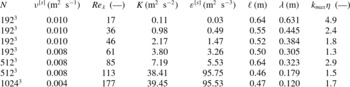
Compilation of the Newtonian DNS results (see the text for definitions). We use SI units for the presented quantities. The box size of the simulations is
 $L_{box}=2{\rm\pi}\ (\text{m})$
.

In the present simulations, the turbulence is sustained by an artificial forcing delta-correlated in time and uncorrelated with the velocity field (Alvelius Reference Alvelius1999). This forcing scheme has the advantage of prescribing a priori the power input spectrum
 $f(k)$
and thus the total power input
 $P$
and to indirectly influence the integral scale
 $\ell$
. We force the first four wavenumbers with a Gaussian profile centred at wavenumber 3 and distributed over the neighbouring wavenumbers 2 and 4 so that there is negligible power input in the first wavenumber and the ratio between the box size and the integral scale ranges between 9 and 14. A set of simulations with
 ${\it\beta}=0.8$
and
 ${\it\tau}=0.4\ \text{s}$
(to compare with run 5 in table 2) were carried out with other forcing parameters, namely (i) concentrated power input at wavenumber 3 and (ii) power input at wavenumbers 1 and 2 in order to ensure that our results did not meaningfully change, particularly concerning the behaviour of the polymer stresses and the spectrum of kinetic energy to elastic energy transfer. We also performed a set of simulations (runs 29 and 30 in table 2) with the ‘acceleration’ forcing used in Lamorgese, Caughey & Pope (Reference Lamorgese, Caughey and Pope2005) applied to wavenumbers 2, 3 and 4, which also allows us to predetermine the power input. This forcing strategy is similar to the linear forcing suggested by Lundgren (Reference Lundgren2003) when the latter is applied to selected wavenumbers.
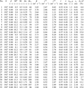
Compilation of the viscoelastic DNS results. We use SI units for the presented quantities (see also table 1). Note that
 $\mathit{Wi}^{0}$
is the polymer relaxation time normalised by the Kolmogorov time scale,
 ${\it\tau}_{{\it\eta}}$
, taken from the reference Newtonian simulation, whereas in the definition of
 $\mathit{Wi}$
the normalising
 ${\it\tau}_{{\it\eta}}$
is taken from the corresponding viscoelastic simulation. For the
 $N=192^{3}$
simulations the solvent viscosity is set to
 ${\it\nu}^{[s]}=0.008\ \text{m}^{2}\ \text{s}^{-1}$
, whereas for the
 $N=384^{3}$
simulations the solvent viscosity is
 ${\it\nu}^{[s]}=0.003\ \text{m}^{2}\ \text{s}^{-1}$
. For all of the simulations the power input is
 $P=3.3\ \text{m}^{2}\ \text{s}^{-3}$
and
 $L^{2}=100^{2}$
(the only exceptions are datasets 9 and 31 where
 $L^{2}=1000^{2}$
and
 $L^{2}=150^{2}$
, respectively). The random forcing delta correlated in time is used for all simulations except runs 32 and 33 where an ‘acceleration’ forcing is used instead (see § 2).

The turbulent kinetic energy
 $K$
, the Newtonian solvent dissipation
 ${\it\varepsilon}^{[s]}$
(the polymer dissipation is treated separately) and the integral scale
 $\ell$
are extracted from the spherical-shell averaged kinetic energy spectrum
 $E(k)$
in the usual way, i.e.
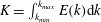 $K=\int _{k_{min}}^{k_{max}}E(k)\text{d}k$
,
 ${\it\varepsilon}^{[s]}=2{\it\nu}^{[s]}\!\int _{k_{min}}^{k_{max}}k^{2}E(k)\text{d}k$
and
 $\ell ={\rm\pi}/(2K)\!\int _{k_{min}}^{k_{max}}E(k)k^{-1}\text{d}k$
, respectively (Monin & Yaglom Reference Monin and Yaglom1975,
 $k_{min}=1$
and
 $k_{max}=\sqrt[3]{N}/3$
are, respectively, the lowest and largest wavenumbers resolved in the simulations). These quantities are used to define the Taylor microscale
 ${\it\lambda}\equiv \sqrt{10{\it\nu}^{[s]}K/{\it\varepsilon}^{[s]}}$
, the Kolmogorov length scale
 ${\it\eta}\equiv ({{\it\nu}^{[s]}}^{3}/{\it\varepsilon}^{[s]})^{1/4}$
, the eddy turnover time
 $\ell /\sqrt{K}$
, the Kolmogorov time scale
 ${\it\tau}_{{\it\eta}}\equiv \sqrt{{\it\nu}^{[s]}/{\it\varepsilon}^{[s]}}$
and the Taylor microscale-based Reynolds number,
 $\mathit{Re}_{{\it\lambda}}\equiv \sqrt{(2/3)K}{\it\lambda}/{\it\nu}^{[s]}$
. Since the turbulence is statistically homogeneous and stationary, the kinetic energy transferred to polymer elastic energy is given by the work of polymer stress against the strain rate,
 ${\it\sigma}_{ij}^{[p]}\unicode[STIX]{x1D61A}_{ij}$
, which is eventually dissipated into heat due to the Stokes frictional drag acting on the polymers, or rather on the dumbbell beads in the FENE model. For the FENE-P model the dumbbell dissipation can be computed as
 ${\it\varepsilon}^{[p]}=f(\unicode[STIX]{x1D60A}_{jj}){\it\sigma}_{ii}^{[p]}/(2{\it\tau})$
(see e.g. Dallas, Vassilicos & Hewitt Reference Dallas, Vassilicos and Hewitt2010). Since our simulations are statistically stationary the kinetic to elastic energy transfer rate balances on average the elastic energy dissipated by the polymers, i.e.
 ${\it\varepsilon}^{[p]}=\overline{{\it\sigma}_{ij}^{[p]}\unicode[STIX]{x1D61A}_{ij}}$
where the overline represents averages in time. We also define a Weissenberg,
 $\mathit{Wi}\equiv {\it\tau}/{\it\tau}_{{\it\eta}}$
, and a Deborah number,
 $\mathit{De}\equiv {\it\tau}\sqrt{K}/\ell$
, i.e. the ratio between the relaxation time and the Kolmogorov and eddy turnover time scales, respectively.
Finally, for reference, we compute Lumley’s length scale (Lumley Reference Lumley1969) characterising the scales where the local eddy turnover time matches the relaxation time of the polymer (i.e. the local Deborah is unity). We do so by computing the kinetic energy structure function averaged over spherical shells
 $\overline{({\it\delta}u_{i})^{2}}(r)\equiv \overline{(u_{i}(\boldsymbol{x}+r)-u_{i}(\boldsymbol{x}))^{2}}$
from the spectrum
 $E(k)$
, since it can be shown that (Monin & Yaglom Reference Monin and Yaglom1975),
 $$\begin{eqnarray}\overline{({\it\delta}u_{i})^{2}}(r)=4\int _{0}^{\infty }\left(1-\frac{\sin kr}{kr}\right)E(k)\text{d}k.\end{eqnarray}$$
(Since we have a periodic domain we effectively compute
 $4\sum _{j=1}^{N}(1-(\sin (k_{j}r_{i}))/(k_{j}r_{i}))$
 $E(k_{j})$
.) From the structure function we compute a local eddy turnover time
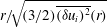 $r/\!\sqrt{\!(3/2)\overline{({\it\delta}u_{i})^{2}}(r)}\!$
and use it to compute
 $r_{L}$
by inverting the relation
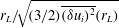 $r_{L}/\!\sqrt{\!(3/2)\overline{({\it\delta}u_{i})^{2}}(r_{L})}$
 $={\it\tau}$
. Note that the factor
 $\sqrt{2/3}$
is added to ensure that
 ${\it\eta}/\sqrt{(3/2)\overline{({\it\delta}u_{i})^{2}}({\it\eta})}=\sqrt{{\it\nu}^{[s]}/{\it\varepsilon}^{[s]}}={\it\tau}_{{\it\eta}}$
, i.e. for
 $r={\it\eta}$
the estimate is compatible with the Kolmogorov time scale (recall that
 $\lim _{r\rightarrow 0}\overline{({\it\delta}u_{i})^{2}}=2{\it\varepsilon}^{[s]}/(3{\it\nu}^{[s]})r^{2}$
).
3. Turbulence in Newtonian fluids at moderate Reynolds numbers
The direct numerical simulations of turbulence in FENE-P fluids are typically one order of magnitude computationally more expensive than their Newtonian counterparts (see e.g. de Angelis et al. Reference de Angelis, Casciola, Benzi and Piva2005; Dallas et al. Reference Dallas, Vassilicos and Hewitt2010) and, consequently, the domain size and currently achievable Reynolds numbers in viscoelastic simulations are moderate. Therefore, we performed first a set of Newtonian DNSs spanning Reynolds numbers from 17 to 177 (see table 1 and caption of figure 1) to study the effect of the Reynolds number on the nonlinear turbulent energy cascade. This will also serve the purpose of reviewing the key aspects of turbulence dynamics in order to better understand the impact of polymer additives.
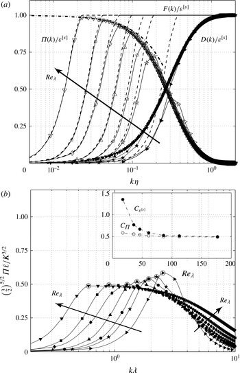
Results from the DNSs of statistically steady homogenous isotropic Newtonian turbulence with (▹
 $|$
▸)
 $\mathit{Re}_{{\it\lambda}}=17$
(✩
 $|$
★)
 $\mathit{Re}_{{\it\lambda}}=36$
, (○
 $|$
●)
 $\mathit{Re}_{{\it\lambda}}=46$
, (▵
 $|$
▴)
 $\mathit{Re}_{{\it\lambda}}=54$
, (♢
 $|$
♦)
 $\mathit{Re}_{{\it\lambda}}=86$
, (▫
 $|$
▪)
 $\mathit{Re}_{{\it\lambda}}=113$
, (▿
 $|$
▾)
 $\mathit{Re}_{{\it\lambda}}=177$
. (a) Spectra of (dashed line)
 $F(k)$
, (empty symbols)
 ${\it\Pi}(k)$
and (filled symbols)
 $D(k)$
. The thick dashed-dotted line follows (3.3) with
 $C_{K}=1.5$
. (b) Spectra of the normalised kinetic energy cascade flux,
 $\left({\textstyle \frac{3}{2}}\right)^{5/2}{\it\Pi}\ell /K^{3/2}$
versus the wavenumber normalised with the Taylor microscale,
 $k{\it\lambda}$
. In the inset we compile the maximum normalised kinetic energy cascade flux,
 $C_{{\it\Pi}}\equiv \max [({\textstyle \frac{3}{2}})^{5/2}{\it\Pi}\ell /K^{3/2}]$
(in open circles) and the normalised energy dissipation
 $C_{{\it\varepsilon}^{[s]}}\equiv \left({\textstyle \frac{3}{2}}\right)^{5/2}{\it\varepsilon}^{[s]}\ell /K^{3/2}$
(in filled circles) and plot them against
 $\mathit{Re}_{{\it\lambda}}$
. The numerical factor
 $\left({\textstyle \frac{3}{2}}\right)^{5/2}$
allows for a direct comparison with experimentally measured surrogates.

The starting point of our analysis is the scale-by-scale power budget in wavenumber space which is the wavenumber space counterpart of the von Kármán–Howarth–Monin equation in physical space (Monin & Yaglom Reference Monin and Yaglom1975). For statistically stationary homogenous turbulence it reads,
 $$\begin{eqnarray}f(k)=-T(k)+2{\it\nu}^{[s]}k^{2}E(k),\end{eqnarray}$$
where
 $k$
is the wavenumber,
 $E(k)$
is the three-dimensional kinetic energy spectrum,
 $T(k)$
is the nonlinear energy transfer spectrum and
 $f(k)$
is the artificial imposed forcing which provides the power input that balances the dissipation. All of the terms in (3.1) are averaged over spherical shells of radius
 $k=|\boldsymbol{k}|$
(thus they include information from the whole computational domain) and averaged in time over about 2–3 eddy turnovers after letting the simulation run for 8–10 eddy turnovers to ensure a fully developed and statistically steady state. The indefinite integral of (3.1) yields
 $$\begin{eqnarray}F(k)={\it\Pi}(k)+D(k),\end{eqnarray}$$
where
 $F(k)\equiv \int _{0}^{k}f(k^{\ast })\text{d}k^{\ast }$
is the power input up to wavenumber
 $k$
,
 ${\it\Pi}(k)\equiv -\!\int _{0}^{k}T(k^{\ast })\text{d}k^{\ast }$
is the net nonlinear energy cascade flux from wavenumbers
 $k^{\ast }\leqslant k$
to larger wavenumbers and
 $D(k)\equiv \int _{0}^{k}2{\it\nu}^{[s]}{k^{\ast }}^{2}E(k^{\ast })\text{d}k^{\ast }$
is the total kinetic energy dissipated up to wavenumber
 $k$
. Clearly, by definition
 $F(k=k_{max})=P$
,
 ${\it\Pi}(k=k_{max})=0$
and
 $D(k=k_{max})={\it\varepsilon}^{[s]}$
. Since the turbulence is statistically stationary all of the power input is, on average, dissipated into heat,
 $P={\it\varepsilon}^{[s]}$
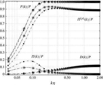
. The three terms of (3.2) are shown in figure 1(a) for various DNS with different levels of
 $\mathit{Re}_{{\it\lambda}}$
(see table 1). The ordinate is normalised by the dissipation (here there is no contribution from the polymers and all of the dissipation is due to the solvent) and the abscissa is normalised by the Kolmogorov microscale
 ${\it\eta}$
so that the increase in Reynolds number is evidenced by the offset to the left of the low-wavenumber part of the spectra. This is most clearly visible for the spectra of external power input and nonlinear energy transfer (cf. figure 1
a).
Note that in DNS, depending on the forcing strategy,
 $f(k)$
is usually prescribed a priori therefore the above equation relates directly
 ${\it\Pi}(k)$
with
 $E(k)$
. For example, for statistically stationary Newtonian turbulence (where
 $P={\it\varepsilon}^{[s]}$
) assuming a Kolmogorov–Obukhov inertial range spectrum,
 $E(k)=C_{K}{{\it\varepsilon}^{[s]}}^{2/3}k^{-5/3}$
, leads to an energy flux spectrum following (Ishihara, Gotoh & Kaneda Reference Ishihara, Gotoh and Kaneda2009),
 $$\begin{eqnarray}{\it\Pi}(k)\simeq P\left(1-\frac{3C_{K}}{2}(k{\it\eta})^{4/3}\right),\quad k>k^{+},\end{eqnarray}$$
where
 $k$
lies within the inertial range and
 $k^{+}$
is the highest wavenumber up to which the forcing is applied so that
 $P\equiv \int _{0}^{\infty }f(k^{\ast })\text{d}k^{\ast }=\int _{0}^{k^{+}}f(k^{\ast })\text{d}k^{\ast }$
. (The relation is not exact because for low wavenumbers the dissipation spectrum no longer follows the same functional form as in the inertial range. Nevertheless, the induced error is asymptotically zero for high Reynolds numbers within Kolmogorov’s phenomenology.) The functional form (3.3) of the cascade flux within the inertial range agrees well with our highest Reynolds number data, see figure 1(a).
Clearly, for statistically stationary turbulence, as
 $\mathit{Re}\rightarrow \infty$
the inertial range flux becomes approximately constant and equal to the dissipation, i.e.
 ${\it\Pi}(k)\simeq {\it\varepsilon}^{[s]}$
. This is the wavenumber space counterpart of the generalised Kolmogorov’s four-fifths law using spherical shell averages rather than kinematic relations based on local isotropy (see Nie & Tanveer Reference Nie and Tanveer1999). However, from (3.3) we infer that
 ${\it\Pi}(k)$
will actually never be exactly constant over a range of wavenumbers since it follows a power-law roll-off. This motivates the characterisation of the inertial range flux by its maximum value
 ${\it\Pi}|_{max}\equiv \max ({\it\Pi})$
which will, nevertheless, become asymptotically equal to the dissipation. At moderate Reynolds numbers
 ${\it\Pi}|_{max}/{\it\varepsilon}^{[s]}$
departs from unity which is sometimes referred to as finite Reynolds number (FRN) effects (Qian Reference Qian1999; Antonia & Burattini Reference Antonia and Burattini2006; Tchoufag, Sagaut & Cambon Reference Tchoufag, Sagaut and Cambon2012).
Although the ratio
 ${\it\Pi}|_{max}/{\it\varepsilon}^{[s]}$
may have significant departures from unity at moderate and low Reynolds numbers, it has been observed by McComb et al. (Reference McComb, Berera, Salewski and Yoffe2010) that the high-Reynolds-number scaling for the flux
 ${\it\Pi}|_{max}$
holds for low Reynolds numbers as well, i.e. that it remains proportional to the kinetic energy times the eddy turnover rate,
 ${\it\Pi}|_{max}\sim K^{3/2}/\ell$
. We test this observation against our data and confirm that it is, indeed, a very good approximation (see figure 1
b). In particular, we plot in the inset of figure 1(b) the non-dimensional group
 $C_{{\it\Pi}}\equiv \left({\textstyle \frac{3}{2}}\right)^{5/2}{\it\Pi}|_{max}\ell /K^{3/2}$
against
 $\mathit{Re}_{{\it\lambda}}$
and observe that even below
 $\mathit{Re}_{{\it\lambda}}\approx 50$
there is only a mild increase on the numerical value of
 $C_{{\it\Pi}}$
in stark contrast to the dissipation normalised in the same way. Note that we have added the numerical factor
 $\left({\textstyle \frac{3}{2}}\right)^{5/2}$
in order to compare our numerical values of
 $C_{{\it\Pi}}$
and
 $C_{{\it\varepsilon}}$
with experimentally measured surrogates. On the basis of isotropy,
 $\sqrt{2K/3}=u^{\prime }$
and
 $\ell =2L_{11}^{(1)}/3$
, where
 $u^{\prime }$
and
 $L_{11}^{(1)}$
are the root-mean-square (r.m.s.) and longitudinal integral length of the velocity fluctuations, typically measured with single hot-wire anemometers. We also confirm that beyond
 $\mathit{Re}_{{\it\lambda}}\gtrapprox 100$
the normalised dissipation
 $C_{{\it\varepsilon}^{[s]}}$
becomes approximately constant and independent on the fluid viscosity. The numerical value of
 $C_{{\it\varepsilon}^{[s]}}\approx 0.5$
is consistent with the values found in the literature for stationary homogenous turbulence (Burattini, Lavoie & Antonia Reference Burattini, Lavoie and Antonia2005).
We use the fact that the scaling reflected in the dimensionless parameter
 $C_{{\it\Pi}}$
holds for low Reynolds numbers as a starting point to analyse the energy cascade in our viscoelastic turbulence simulations where the Reynolds numbers are moderate at best.
4. Global statistics for the viscoelastic simulations
The numerical code described in § 2 is used to perform various simulations with different rheological parameters ranging
 ${\it\tau}=0.025{-}1.0\ \text{s}$
,
 ${\it\beta}=[0.8,0.9,0.95]$
and
 $L^{2}=100^{2}$
for all except two simulations. The range of relaxation times matches roughly that used in the experimental study of the MPI Göttingen group (Ouellette, Xu & Bodenschatz Reference Ouellette, Xu and Bodenschatz2009; Xi et al.
Reference Xi, Bodenschatz and Xu2013) using polyacrylamide in weight concentrations up to 20 p.p.m. (equivalent to
 ${\it\beta}\geqslant 0.9$
;
 $L^{2}=150^{2}$
for polyacrylamide which is of the same order as that used in our simulations,
 $L^{2}=100^{2}$
). We also perform simulations with
 ${\it\beta}=0.8$
which would correspond to the previously mentioned experiments with a polymer mass fraction of approximately 45 p.p.m. (To estimate the corresponding concentration we compute the ‘
 ${\it\beta}$
concentration’,
 $c_{{\it\beta}}=(1-{\it\beta})/{\it\beta}$
, which can be estimated as
 $c_{{\it\beta}}=(ck_{B}T{\it\tau})/({\it\nu}^{[s]}M_{p})$
(Jin Reference Jin2007), where
 $c,k_{B},T,M_{p}$
are the polymer mass fraction, Boltzmann’s constant, the temperature of the solution and mass of a single polymer molecule, respectively.) Polymers solutions with these concentrations can still be considered dilute, since the overlap concentration (an estimate characterising the onset of polymer chain overlap) for polyacrylamide solutions in water is
 $c^{\star }\approx 200\ \text{p.p.m.}$
, see e.g. Liu, Jun & Steinberg (Reference Liu, Jun and Steinberg2009).
Most of the simulations are performed with
 $N=192^{3}$
collocation points and the straddled
 $\mathit{Re}_{{\it\lambda}}$
is small (see table 2). In addition we perform simulations with
 $N=384^{3}$
and a larger
 $\mathit{Re}_{{\it\lambda}}$
for
 ${\it\beta}=0.8$
and
 ${\it\tau}=[0.2,0.4,0.8]$
in order to infer on the qualitative effect of the Reynolds number (datasets 29–31 in table 2; in dataset 31 we set
 $L^{2}=150^{2}$
to avoid excessive polymer extension relative to
 $L^{2}$
and thus numerical instabilities). We also perform an additional simulation with
 ${\it\beta}=0.8$
and
 ${\it\tau}=0.6$
, but
 $L^{2}=1000^{2}$
, in order to assess the effect of finite extensibility of the polymers (dataset 9 in table 2). Finally we perform two additional simulations using the ‘acceleration’ forcing of Lamorgese et al. (Reference Lamorgese, Caughey and Pope2005) (see § 2) with
 ${\it\beta}=0.8$
and
 ${\it\tau}=[0.6,1.0]$
, in order to assess the influence of the forcing on our results (datasets 32 and 33 in table 2). Note that the resolution of our simulations varies between
 $k_{max}{\it\eta}=1.3{-}2.2$
(see table 2), which previous works have reported to be sufficient (Perlekar et al.
Reference Perlekar, Mitra and Pandit2010; Robert et al.
Reference Robert, Vaithianathan, Collins and Brasseur2010). Nevertheless, we performed a simulation with the input parameters of dataset 6 using
 $N=384^{3}$
collocation points (thus
 $k_{max}{\it\eta}=4.0$
) and confirmed that the differences in the statistics considered here are negligibly small.
4.1. Polymer and solvent dissipation
We start by characterising the fraction of the power input dissipated by the solvent and by the polymers for the various
 ${\it\tau}$
(normalised as
 $\mathit{De}$
or
 $\mathit{Wi}$
) and
 ${\it\beta}$
. As expected, for
 $\mathit{Wi}\lessapprox 1$
(
 $\mathit{De}\lessapprox 0.2$
in our simulations, see table 2 and figure 2
a) the fraction of the power input dissipated by the solvent is approximately equal to the numerical value of the parameter
 ${\it\beta}$
since elasticity plays a weak role and a Newtonian behaviour is recovered with total viscosity
 ${\it\nu}^{[s]}+{\it\nu}^{[p]}={\it\nu}^{[s]}/{\it\beta}$
(Bird, Armstrong & Hassager Reference Bird, Armstrong and Hassager1987a
; Bird et al.
Reference Bird, Curtiss, Armstrong and Hassager1987b
). For increasing
 $\mathit{De}$
(noting that
 $\mathit{Wi}\gtrapprox 1$
such that the polymers are stretched by the flow) we observe that the polymers dissipate an increasingly larger fraction of the power input leading to a depletion of the solvent dissipation and thus of fine-scale structures (figure 2
a). This is in line to what has been previously reported in the literature (de Angelis et al.
Reference de Angelis, Casciola, Benzi and Piva2005; Perlekar, Mitra & Pandit Reference Perlekar, Mitra and Pandit2006; Liberzon et al.
Reference Liberzon, Holzner, Lüthi, Guala and Kinzelbach2009; Ouellette et al.
Reference Ouellette, Xu and Bodenschatz2009; Cai et al.
Reference Cai, Li and Zhang2010; Perlekar et al.
Reference Perlekar, Mitra and Pandit2010; Horiuti et al.
Reference Horiuti, Matsumoto and Fujiwara2013; Xi et al.
Reference Xi, Bodenschatz and Xu2013). Concomitantly, the fraction of power dissipated by the polymers,
 ${\it\varepsilon}^{[p]}/P$
, increases substantially and can be as high as 90 % of the total power input as can be seen in our
 $N=384^{3}$
simulation with
 $\mathit{Re}_{{\it\lambda}}\approx 160$
,
 $\mathit{De}\approx 0.9$
and
 ${\it\beta}=0.8$
(dataset 30 in table 2, see also figure 2
a). Although large values of
 ${\it\varepsilon}^{[p]}/P$
have been reported in the literature they typically do not exceed
 ${\it\varepsilon}^{[p]}/P\approx 70\,\%$
(see the data compilation by Liberzon et al.
Reference Liberzon, Holzner, Lüthi, Guala and Kinzelbach2009). The larger values yielded by some of our simulations are likely due to the fact that our simulations span values of the Deborah number (i.e. the ratio between
 ${\it\tau}$
and the turnover time) that are also larger than those straddled previously. Note that both types of external forcing produce a similar fraction of power dissipated by the polymers (see figure 2
a). For large polymer relaxation times (
 $\mathit{De}\gtrapprox 1$
) there is a decrease in the fraction of the power dissipated by the polymers. This is likely a consequence of the fact that the average polymer dissipation (
 ${\it\varepsilon}^{[p]}\equiv (1/V)\int _{V}f(\unicode[STIX]{x1D60A}_{ii}){\it\sigma}_{ii}^{[p]}/(2{\it\tau})\text{d}V$
in the FENE-P model, where
 $V=(2{\rm\pi})^{3}$
is the volume of the computational box) is directly proportional to the average trace of the polymer stress,
 ${\it\sigma}_{ii}^{[p]}$
, and inversely proportional to the relaxation time,
 ${\it\tau}$
. In other words, for increasingly large
 $\mathit{De}$
, the increase in polymer stress due to larger polymer elongations (
 $\unicode[STIX]{x1D60A}_{ii}$
) does not compensate for the effect of the increased relaxation time in reducing the polymer dissipation. In wall-bounded turbulence, Dallas et al. (Reference Dallas, Vassilicos and Hewitt2010) also showed that the total polymer dissipation grows with the polymer relaxation time up to a point where it starts to decrease. The former regime is characterised by low drag reduction, whereas the latter by high (or maximum) drag reduction.
Global statistics from the DNSs of statistically steady homogenous isotropic viscoelastic turbulence versus the Deborah number. Datasets 1–28, excluding dataset 9 (
 $N=192^{3}$
with the delta-correlated forcing and
 $L^{2}=100^{2}$
, see table 2) for the different solvent to total viscosity ratios are plotted with (●
 $|$
○)
 ${\it\beta}=0.8$
, (▪
 $|$
▫)
 ${\it\beta}=0.9$
, (▵
 $|$
▴)
 ${\it\beta}=0.95$
. Datasets 29–31 with higher Reynolds number (see table 2) are plotted with (

 $|$

 $|$
✩). In (a) the open symbols show the percentage of the solvent dissipation over the total power input,
 ${\it\varepsilon}^{[s]}/P$
and the filled symbols show the percentage of the polymer dissipation over the total power input,
 ${\it\varepsilon}^{[p]}/P$
. In (b) the open symbols show the normalised energy dissipation,
 $C_{{\it\varepsilon}^{[s]}}$
and the filled symbols show the power input normalised in the same way,
 $C_{P}$
.

Perhaps surprisingly, however, there is only a mild dependence of the fraction of polymer dissipation on the polymer viscosity parameter,
 ${\it\beta}$
. This implies that increasing
 ${\it\beta}$
, which corresponds to a decrease in the polymer zero-shear-rate viscosity, turns out to be concomitant with an increase in the mean square dumbbell separation
 $\unicode[STIX]{x1D60A}_{ii}$
(cf. table 2) so that the kinetic energy to elastic energy transfer rate (and, thus, polymer dissipation) only mildly changes (figure 2
a). This appears to be consistent with the argument presented by Balbovsky et al. (Reference Balbovsky, Fouxon and Lebedev2001) whereby the characteristic elongation of the molecules is such that the polymer stresses are of the order of the viscous stresses (because beyond this point they modify the surrounding flow and diminish stretching). Recall that the polymer stresses are proportional to the elongation and the zero-shear-rate viscosity (which in turn is related to the concentration of the polymers). In figure 2(a) we also present the data from the higher-Reynolds-number simulations which are qualitatively similar, albeit the fraction of total power dissipated by the polymers is slightly larger.
Since the polymers add a source of dissipation which also leads to changes in the kinetic energy of the flow and the integral scale (see table 2), it is not straightforward to compare Newtonian and viscoelastic dissipation routes without appropriately normalising the quantities. Therefore, we normalise the power input and dissipation by the solvent with the kinetic energy,
 $K$
and eddy turnover time
 $\ell /\sqrt{K}$
as it is customary for Newtonian turbulence (see § 3) and form the non-dimensional groups
 $C_{P}\equiv \left({\textstyle \frac{3}{2}}\right)^{5/2}P\ell /K^{3/2}$
and
 $C_{{\it\varepsilon}^{[s]}}\equiv \left({\textstyle \frac{3}{2}}\right)^{5/2}{\it\varepsilon}^{[s]}\ell /K^{3/2}$
. Note that, in some sense,
 $C_{P}$
(
 $=C_{{\it\varepsilon}^{[s]}}$
in statistically steady Newtonian turbulence) measures the efficiency of turbulence in dissipating the power input for a given large-scale flow. In figure 2(b) we plot
 $C_{{\it\varepsilon}^{[s]}}$
as a function of
 $\mathit{De}$
for the three different values of the parameter
 ${\it\beta}$
. We observe that up to
 $\mathit{De}\approx 0.7$
the normalised solvent dissipation
 $C_{{\it\varepsilon}^{[s]}}$
decreases to half of its numerical value in the Newtonian reference case which may be interpreted as a decrease in the efficiency of the turbulence to dissipate energy through the solvent. For larger
 $\mathit{De}$
, however,
 $C_{{\it\varepsilon}^{[s]}}$
increases and, for the largest
 $\mathit{De}$
and lowest
 ${\it\beta}$
it exceeds the numerical value of the Newtonian reference. If we, instead, consider the normalised power input
 $C_{P}$
we observe that for large
 $\mathit{De}$
its numerical value can be as high as five times the one typically found in Newtonian turbulence. Recall that we keep the total power input constant for all simulations (which is the sum of the solvent plus polymer dissipation due to stationarity) and therefore the large increase in
 $C_{P}$
is mainly due to a substantial decrease in the kinetic energy
 $K$
and a mild increase in the integral scale
 $\ell$
(see table 2). Once more, the trend for the higher-Reynolds-number simulations is qualitatively the same even though
 $C_{{\it\varepsilon}^{[s]}}$
and
 $C_{P}$
have smaller numerical values (see figure 2
b).
4.2. Scale-by-scale kinetic energy transfer balance
Similarly to the approach taken for the analysis of Newtonian fluid turbulence we write the scale-by-scale power balance equation modified to include the wavenumber breakdown of the net kinetic energy transferred to/from the polymer elastic energy which we denote as
 $T^{[p]}(k)$
(see e.g. Brasseur et al.
Reference Brasseur, Robert, Collins and Vaithianathan2005; Casciola & de Angelis Reference Casciola and de Angelis2007). In essence it is the spectral decomposition of the work produced from the interaction of the polymer stresses with the strain rate. The equation reads
 $$\begin{eqnarray}f(k)=-T(k)+T^{[p]}(k)+2{\it\nu}^{[s]}k^{2}E(k).\end{eqnarray}$$
Note that the integral of
 $T^{[p]}(k)$
is the total energy transferred to/from the polymer which in statistically stationary turbulence is equal to the elastic energy dissipated by the polymers and therefore a strictly positive quantity, i.e.
 $\int _{0}^{\infty }T^{[p]}(k)\text{d}k>0$
. However,
 $T^{[p]}(k)$
can be positive or negative at different wavenumbers representing a transfer of kinetic to elastic energy or from elastic to kinetic energy, respectively. Thus,
 $T^{[p]}(k)$
can be thought of as distributed kinetic energy sources/sinks at the different wavenumbers but whose net effect over all scales is to remove kinetic energy from the solvent reflecting the dissipative nature of the polymers as they stretch and recoil.
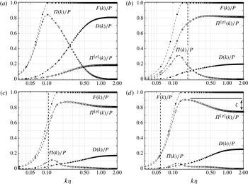
We plot the indefinite integral of (4.1),
 $$\begin{eqnarray}F(k)={\it\Pi}(k)+{\it\Pi}^{[p]}(k)+D(k)\end{eqnarray}$$
for four different
 $\mathit{De}$
in figure 3. The new term,
 ${\it\Pi}^{[p]}(k)\equiv \int _{0}^{k}T^{[p]}(k^{\ast })\text{d}k^{\ast }$
represents the total kinetic to elastic energy transfer up to wavenumber
 $k$
and, as expected, shows a strong dependence on the polymer relaxation time. For
 $\mathit{Wi}\lessapprox O(1)\ (\mathit{De}\lessapprox 0.2)$
we confirmed that
 ${\it\Pi}^{[p]}(k)$
becomes proportional to the solvent’s dissipation spectrum, i.e.
 ${\it\Pi}^{[p]}(k)\approx (1/{\it\beta}-1)D(k)$
indicating that the polymer solution behaves as a Newtonian fluid with total viscosity
 ${\it\nu}^{[s]}+{\it\nu}^{[p]}$
(figure 3
a; see also figure 2
a). For higher
 $\mathit{Wi}$
(and
 $\mathit{De}$
), however, the kinetic to elastic energy transfer
 ${\it\Pi}^{[p]}(k)$
becomes the dominant kinetic energy loss mechanism and we can observe that for cases with
 $\mathit{De}\geqslant 0.7$
it also overcomes the power exchanges via the nonlinear energy cascade for all wavenumbers (cf. figure 3
b–d). In fact, for the cases with
 $\mathit{De}=[1.17,2.14]$
almost all of the external power input goes directly to the polymers (figure 3
c,d).
Spectral energy transfer budget, (4.2), for the DNSs of statistically steady homogenous isotropic viscoelastic turbulence for
 ${\it\beta}=0.8$
and (a)
 $\mathit{De}=0.1\ (\mathit{Wi}=0.5)$
, (b)
 $\mathit{De}=0.71\ (\mathit{Wi}=2.7)$
, (c)
 $\mathit{De}=1.17\ (\mathit{Wi}=5.1)$
and (d)
 $\mathit{De}=2.14\ (\mathit{Wi}=10.2)$
. Legend: (●)
 $F(k)/P$
; (▫)
 ${\it\Pi}(k)/P$
; (○)
 ${\it\Pi}^{[p]}(k)/P$
; (▸)
 $D(k)/P$
. The vertical thick dashed line represents the wavenumber corresponding to the Lumley scale,
 $r_{L}$
added for reference. In (d) the polymer-induced energy cascade
 ${\it\zeta}$
is depicted.

As a consequence, the maximum nonlinear energy cascade flux,
 ${\it\Pi}|_{max}$
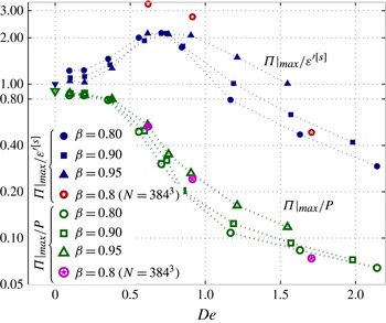
is a monotonically decreasing fraction of the power input for increasing
 $\mathit{De}$
and for all
 ${\it\beta}$
(see figure 4). However, since the solvent dissipation also decreases we compare the ratio between the two in figure 4. Note that, to negotiate the confounding effect of having non-zero dissipation at large scales due to FRN (see § 3) we consider only the solvent dissipation for wavenumbers larger than the wavenumber
 $k^{\star }$
of maximum nonlinear energy transfer (such that
 ${\it\Pi}(k^{\star })\equiv {\it\Pi}|_{max}$
), i.e.
 ${\it\varepsilon}^{\prime [s]}\equiv 2{\it\nu}^{[s]}\int _{k^{\star }}^{\infty }k^{2}E(k)\text{d}k$
. It turns out that the cascade flux exceeds the solvent dissipation, i.e.
 ${\it\Pi}|_{max}/{\it\varepsilon}^{\prime [s]}>1$
, for
 $\mathit{De}\lessapprox 1.0$
. This highlights the fact that the energy being transferred from low to high wavenumbers goes both to the solvent, which is then dissipated by the fine turbulence eddies, and to the polymer chains, which also dissipate it as the polymers stretch and recoil. Contrastingly, for
 $\mathit{De}\gtrapprox 1.0$
the energy cascade flux becomes smaller than the solvent dissipation, i.e.
 ${\it\Pi}|_{max}/{\it\varepsilon}^{\prime [s]}<1$
, and thus there must be an additional energy transfer route that accounts for the difference. It turns out that this energy cascade route is provided by the polymers via the term
 ${\it\Pi}^{[p]}(k)$
. As can be seen in figure 3(c,d),
 ${\it\Pi}^{[p]}(k)$
has a maximum at some intermediate wavenumber and decreases up to the highest wavenumber, indicating a sign change in the kinetic energy to elastic energy transfer spectrum
 $T^{[p]}(k)$
. This implies that the polymers extract more kinetic energy from the large scales than they can dissipate and return the difference to the large wavenumbers, i.e. the fine scales. To the best of the authors’ knowledge, this is the first data clearly showing a polymer-induced kinetic energy cascade owing to the net transfer of elastic to kinetic energy at large wavenumbers. Note, however, that a careful examination of figure 6 in Brasseur et al. (Reference Brasseur, Robert, Collins and Vaithianathan2005) and figure 22 in Watanabe & Gotoh (Reference Watanabe and Gotoh2013) also indicate the onset of a high-wavenumber elastic-to-kinetic energy transfer. We define a parameter
 ${\it\zeta}\equiv \max ({\it\Pi}^{[p]}(k))-{\it\Pi}^{[p]}(\infty )$
(effectively, due to discretisation we compute
 ${\it\zeta}=\max ({\it\Pi}^{[p]}(k))-{\it\Pi}^{[p]}(k_{max})$
) which quantifies the total cascade flux induced by the polymers (see figure 3
d for a graphical representation of
 ${\it\zeta}$
). This parameter is useful to characterise the scaling of the total energy transferred from large to small scales.
Ratio between the maximum energy cascade flux and the power input,
 ${\it\Pi}|_{max}/P$
, or the small-scale solvent dissipation,
 ${\it\Pi}|_{max}/{\it\varepsilon}^{\prime [s]}$
versus the Deborah number for all DNS data (see the text for the definition of
 ${\it\varepsilon}^{\prime [s]}$
and note that the ordinates are logarithmically spaced). Legend:
 ${\it\beta}=0.8$
,
 ${\it\beta}=0.9$
,
 ${\it\beta}=0.95$
and
 ${\it\beta}=0.8\ (N=384^{3})$
represent datasets 1–11 (excluding dataset 9), 12–20, 21–28 and 29–31, respectively.

This polymer-induced energy cascade is also manifested in our larger-Reynolds-number simulations (see figure 5
a). Although, the Reynolds numbers spanned by our simulations are insufficient to infer on the behaviour of viscoelastic inertial turbulence at high Reynolds numbers, our DNS nevertheless show that the polymer-induced energy cascade
 ${\it\zeta}$
and the large fraction of energy dissipation by the polymers occur at moderate Reynolds numbers.
(a) Effect of Reynolds number on the spectral transfer budget from the comparison between two datasets (6 and 30 in table 2) with the same
 ${\it\beta}=0.8$
and
 ${\it\tau}=0.4\ \text{s}$
(and, thus, similar Deborah
 $\mathit{De}=0.84$
and
 $\mathit{De}=0.91$
, respectively) but different
 ${\it\nu}^{[s]}$
such that
 $\mathit{Re}_{{\it\lambda}}=72$
and
 $\mathit{Re}_{{\it\lambda}}=160$
, respectively. (b) Effect of maximum polymer extensibility on the spectral transfer budget from the comparison between two datasets (8 and 9 in table 2) with the same
 ${\it\beta}=0.8$
and
 ${\it\tau}=0.6\ \text{s}$
(and, thus, similar Deborah
 $\mathit{De}\approx 1.2$
) but different
 $L^{2}$
such that
 $\unicode[STIX]{x1D60A}_{ii}/L^{2}=7.6\ [\%]$
and
 $\unicode[STIX]{x1D60A}_{ii}/L^{2}=0.1\ [\%]$
, respectively. Legend: (★
 $|$

 $F(k)/P$
; (▪
 $|$

 ${\it\Pi}(k)/P$
; (●
 $|$

 ${\it\Pi}^{[p]}(k)/P$
; (▸
 $|$

 $D(k)/P$
. Open circles have been overlaid in the datasets with larger
 $\mathit{Re}_{{\it\lambda}}$
and
 $L^{2}$
(datasets 30 and 9, respectively).

We also note that the physical mechanism behind the polymer-induced energy cascade
 ${\it\zeta}$
, is not due to the nonlinear finite extensibility springs of the FENE-P model. This is inferred by comparing the results of the DNS with
 $\mathit{De}=1.2$
,
 ${\it\beta}=0.8$
and
 $L^{2}=100^{2}$
(dataset 8 in table 2) with a second DNS where the maximum squared extensibility is increased to
 $L^{2}=1000^{2}$
(dataset 9 in table 2) so that the Peterlin function is always very close to unity (even instantaneously for any point in the domain) and the FENE-P chains effectively behave as linear springs just like in the Oldroyd-B model. The wavenumber power balance (4.2) for the two DNSs is compared in figure 5(b) where it can be seen that there are very small quantitative differences and the overall behaviour is very similar. Finally, we show the results for the two DNSs with the ‘acceleration’ forcing to show that the polymer-induced energy cascade is not particular to the delta-correlated forcing (see figure 6).
Spectral transfer budget for the DNSs with the ‘acceleration’ forcing at two Deborah numbers,
 $\mathit{De}=0.94$
(dataset 32) and
 $\mathit{De}=1.35$
(dataset 33). See the caption of figure 5 for the legend noting that now open circles overlaid on the symbols depict spectra from dataset 33. See table 2 for further details on the datasets.

So far we have shown that the polymers induce severe changes in the turbulent energy cascade as well as inducing a kinetic energy cascade of their own for large
 $\mathit{De}$
. However, as we saw for the Newtonian simulations, the scaling of the nonlinear energy cascade flux with large-scale quantities
 $K$
and
 $\ell$
is quite robust and was only weakly dependent on the Reynolds number leading to
 $C_{{\it\Pi}}\approx \text{const.}$
(see the inset to figure 1
b). We now test the same scaling for the viscoelastic simulations as a function of the rheological parameters (see figure 7
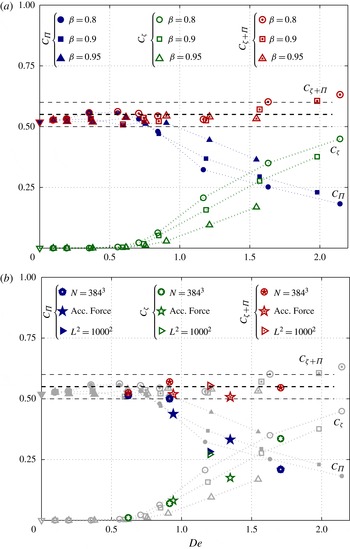
a). Indeed, up to
 $\mathit{De}\approx 0.7$
the numerical value of
 $C_{{\it\Pi}}$
is very close to the Newtonian reference,
 $C_{{\it\Pi}}\approx 0.5$
, even though for
 $\mathit{De}\approx 0.7$
the polymers already dissipate more than 80 % of the power input (see figure 2
a and table 2). For larger
 $\mathit{De}$
the numerical value of
 $C_{{\it\Pi}}$
decreases, which corresponds to the onset of the kinetic energy cascade due to the polymers (for convenience we form the dimensionless parameter
 $C_{{\it\zeta}}\equiv \left({\textstyle \frac{3}{2}}\right)^{5/2}{\it\zeta}\ell /K^{3/2}$
). Remarkably, the sum of the two kinetic energy cascade fluxes turns out to amount roughly to the same fraction of
 $K^{3/2}/\ell$
as in the Newtonian reference case, i.e.
 $C_{{\it\Pi}+{\it\zeta}}\equiv \left({\textstyle \frac{3}{2}}\right)^{5/2}({\it\zeta}+{\it\Pi}|_{max})\ell /K^{3/2}\approx 0.5$
for the range of
 $\mathit{De}$
and
 ${\it\beta}$
spanned by our simulations (see figure 7
a). It is apparent, nevertheless, that there is a mild increase in the sum of
 $C_{{\it\Pi}}$
and
 $C_{{\it\zeta}}$
, denoted as
 $C_{{\it\Pi}+{\it\zeta}}$
, for the larger Deborah numbers. Note that the normalised solvent dissipation and power input scale in a very different way (cf. figure 2
b) and thus there is no reason a priori to expect the constancy of
 $C_{{\it\Pi}+{\it\zeta}}$
which, to the best of the authors’ knowledge, is presented here for the first time. This observation is further strengthened by the fact that the larger Reynolds number simulations (up
 $\mathit{Re}_{{\it\lambda}}\leqslant 183$
) as well as the simulation with the ‘acceleration’ forcing behave in a consistent way (see figure 7
b).
Normalised maximum nonlinear energy cascade flux,
 $C_{{\it\Pi}}$
, polymer-induced kinetic energy cascade flux,
 $C_{{\it\zeta}}$
and total kinetic energy cascade flux,
 $C_{{\it\Pi}+{\it\zeta}}$
versus the Deborah number for all DNS data. In (a) only the runs with delta-correlated forcing,
 $N=192^{3}$
and
 $L^{2}=100^{2}$
are presented (datasets 1–28, excluding dataset 9 in table 2). The same data are presented in (b) in light grey together with the remaining DNS data which are ran with
 ${\it\beta}=0.8$
and we use to test (i) the effect of increasing the Reynolds number (labelled ‘
 $N=384^{3}$
’: datasets 29–31 in table 2), (ii) the effect changing the large-scale forcing (labelled ‘Acc. Force’: datasets 32 and 33 in table 2) and (iii) the effect of increasing the maximum extensibility (labelled ‘
 $L^{2}=1000^{2}$
’: dataset 9 in table 2).

5. Discussion
In the previous section (§ 4) we presented data showing that, for large Deborah numbers, the polymers induce a kinetic energy cascade by removing more kinetic energy from the low-wavenumber range than they can dissipate and returning the excess energy into high wavenumbers. This energy transfer may bear some resemblance to the mechanism in drag-reduced wall bounded turbulence whereby polymers extract turbulent kinetic energy from the flow closer to the wall, store it as elastic energy (
 ${\it\sigma}_{ij}^{[p]}\unicode[STIX]{x1D61A}_{ij}>0$
) and transfer part of this energy back further away from the wall (Min et al.
Reference Min, Yoo, Choi and Joseph2003; Dubief et al.
Reference Dubief, White, Terrapon, Shaqfeh, Moin and Lele2004; Dallas et al.
Reference Dallas, Vassilicos and Hewitt2010; Dubief et al.
Reference Dubief, Terrapon and Soria2013). However, in the present spatially homogeneous flows
 ${\it\sigma}_{ij}^{[p]}\unicode[STIX]{x1D61A}_{ij}$
is, on average, the same everywhere and must be positive due to the dissipative nature of the polymers. Therefore, only local fluctuations can lead to an elastic to kinetic energy transfer, i.e.
 ${\it\sigma}_{ij}^{[p]}\unicode[STIX]{x1D61A}_{ij}<0$
.
It may seem counter-intuitive that the polymers remove most of the kinetic energy from the large instead of the small scales which are typically associated with larger strain rates. However, as commented by Terrapon et al. (Reference Terrapon, Dubief, Moin, Shaqfeh and Lele2004): ‘even a strong flow will not unravel a polymer molecule if it does not last long enough’. Therefore, it appears that the weak but persistent strain rate from the large scales becomes increasingly effective in unravelling the polymer molecules for large
 $\mathit{De}$
, whereas the stronger but short lived small-scale gradients become decreasingly effective. In fact, our data indicate a loss of correlation/alignment between the polymer stress tensor and the strain rate tensor for large Deborah numbers. This can be seen, for example, in figure 2 where we show the polymer dissipation decreasing for
 $\mathit{De}>1$
in the runs with
 ${\it\beta}=[0.8,0.9]$
(recall that on average
 ${\it\varepsilon}^{[p]}={\it\sigma}_{ij}^{[p]}\unicode[STIX]{x1D61A}_{ij}$
in statistically steady polymer-laden turbulence), even though the trace of the polymer stress tensor (
 $\propto \unicode[STIX]{x1D60A}_{ii}$
) as well as
 $\unicode[STIX]{x1D61A}_{ij}\unicode[STIX]{x1D61A}_{ij}\ (\propto {\it\varepsilon}^{[N]})$
monotonically increase for
 $\mathit{De}>1$
(see table 2 and figure 2). This appears to be a common feature of polymer-laden flows at moderate to large Deborah (or Weissenberg) numbers since similar findings were reported by Brasseur et al. (Reference Brasseur, Robert, Collins and Vaithianathan2005) in homogeneous shear turbulence (see their figure 6) and by Watanabe & Gotoh (Reference Watanabe and Gotoh2013) for homogeneous decaying turbulence (see their figures 11 and 22).
Probability of alignment between the principal axes (a,c,e)
 $\unicode[STIX]{x1D628}_{j}^{(1)}$
and (b,d,f)
 $\unicode[STIX]{x1D628}_{j}^{(2)}$
(corresponding to the largest and intermediate eigenvalue) of the polymer stress tensor with the principal axes of the strain-rate tensor for three simulations with (a,b)
 $\mathit{De}=0.19$
, (c,d)
 $\mathit{De}=0.56$
and (e,f)
 $\mathit{De}=2.14$
(datasets 2, 4 and 11 in table 2, respectively). The probability distributions are individually normalised such that they integrate to unity.

We confirmed the loss of alignment between
 $\unicode[STIX]{x1D61A}_{ij}$
and
 ${\it\sigma}_{ij}^{[p]}$
by computing the cosine between the three principal axes of the strain-rate tensor
 $\unicode[STIX]{x1D626}_{j}^{(1)}$
,
 $\unicode[STIX]{x1D626}_{j}^{(2)}$
and
 $\unicode[STIX]{x1D626}_{j}^{(3)}$
and the principal axes of the polymer stress tensor
 $\unicode[STIX]{x1D628}_{j}^{(1)}$
,
 $\unicode[STIX]{x1D628}_{j}^{(2)}$
and
 $\unicode[STIX]{x1D628}_{j}^{(3)}$
in the spirit of the extensive work done for vorticity and scalar gradient alignments in turbulence (see e.g. Ashurst et al.
Reference Ashurst, Kerstein, Kerr and Gibson1987; Jimenez Reference Jimenez1992; Tsinober, Kit & Dracos Reference Tsinober, Kit and Dracos1992). Since we seek the alignment between two tensors, there are 9 inner products between their principal axes appearing in the Frobenius product
 ${\it\sigma}_{ij}^{[p]}\unicode[STIX]{x1D61A}_{ij}$
, i.e.
 $$\begin{eqnarray}{\it\sigma}_{ij}^{[p]}\unicode[STIX]{x1D61A}_{ij}={\it\lambda}^{(i)}{\it\xi}^{(\,j)}\cos ^{2}\left(e_{k}^{(i)},g_{k}^{(\,j)}\right),\end{eqnarray}$$
where
 ${\it\lambda}^{(i)}$
and
 ${\it\xi}^{(i)}$
are the eigenvalues corresponding to the eigenvectors
 $\unicode[STIX]{x1D626}_{j}^{(i)}$
and
 $\unicode[STIX]{x1D628}_{j}^{(i)}$
, respectively. Note that, in contrast to the eigenvalues of the strain-rate tensor which add to zero and therefore it is customary to sort them such that the first (third) is always positive (negative) whereas the intermediate can either be positive or negative for different flow regions, the eigenvalues of the polymer stress tensor are always non-negative since the tensor is positive semidefinite (Jin & Collins Reference Jin and Collins2007). For convenience we also sort the eigenvalues of the polymer stress tensor such that
 ${{\it\xi}_{j}}^{(1)}\geqslant {{\it\xi}_{j}}^{(2)}\geqslant {{\it\xi}_{j}}^{(3)}$
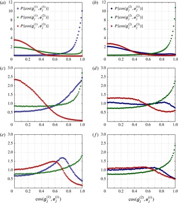
. In figure 8 we present the alignment between
 $\unicode[STIX]{x1D628}_{j}^{(1)}$
as well as
 $\unicode[STIX]{x1D628}_{j}^{(2)}$
with the three principal axes of the strain-rate tensor for three simulations with
 $\mathit{De}=[0.19,0.56,2.14]$
(datasets 2, 4 and 11 in table 2). (We do not present the graphs showing the alignment of
 $\unicode[STIX]{x1D628}_{j}^{(3)}$
since its corresponding eigenvalue is much smaller than the other two and therefore does not significantly contribute to
 ${\it\sigma}_{ij}^{[p]}\unicode[STIX]{x1D61A}_{ij}$
.) We choose these three datasets to represent different types of polymer-turbulence interactions, namely (i)
 $\mathit{De}=0.19$
, a passive polymer-laden turbulent flow, where
 ${\it\sigma}_{ij}^{[p]}\unicode[STIX]{x1D61A}_{ij}\sim \unicode[STIX]{x1D61A}_{ij}\unicode[STIX]{x1D61A}_{ij}$
, see § 4; (ii)
 $\mathit{De}=0.56$
, a turbulent flow where the polymers dissipate 70 % of the power input but do not induce a kinetic energy cascade (i.e.
 ${\it\zeta}\approx 0$
); and (iii)
 $\mathit{De}=2.14$
, a turbulent flow where the polymers dissipate 75 % of the power input and induce a strong kinetic energy cascade flux
 ${\it\zeta}$
which is greater than twice the nonlinear kinetic energy cascade
 ${\it\Pi}|_{max}$
(see figure 7
a). There are two main outstanding features that can be observed. First, the intermediate eigenvector of the polymer stress tensor,
 $\unicode[STIX]{x1D628}_{j}^{(2)}$
, is always preferentially aligned with the intermediate eigenvector of the strain-rate tensor,
 $\unicode[STIX]{x1D626}_{j}^{(2)}$
, for all three datasets, showing a consistent behaviour. In stark contrast, the eigenvector corresponding to the largest eigenvalue,
 $\unicode[STIX]{x1D628}_{j}^{(1)}$
, has different preferential alignments for the three datasets. For the lowest
 $\mathit{De}$
,
 $\unicode[STIX]{x1D628}_{j}^{(1)}$
is preferentially aligned with
 $\unicode[STIX]{x1D626}_{j}^{(1)}$
as expected, but for the intermediate
 $\mathit{De}$
it preferentially aligns with either
 $\unicode[STIX]{x1D626}_{j}^{(1)}$
or
 $\unicode[STIX]{x1D626}_{j}^{(2)}$
. Outstandingly, however, for the largest
 $\mathit{De}$
, the statistics are dramatically different showing the same preferential alignment with
 $\unicode[STIX]{x1D626}_{j}^{(2)}$
but also alternative preferred configurations with angles of 45° and 55° (
 ${\approx}\cos ^{-1}(0.7)$
and
 ${\approx}\cos ^{-1}(0.65)$
, respectively) with
 $\unicode[STIX]{x1D626}_{j}^{(1)}$
and
 $\unicode[STIX]{x1D626}_{j}^{(3)}$
, respectively. The latter alignment, which can lead to
 ${\it\sigma}_{ij}^{[p]}\unicode[STIX]{x1D61A}_{ij}<0$
(since
 ${\it\lambda}^{(3)}<0$
) may be the underlying cause of the polymer-induced kinetic energy cascade. We also repeated the above analysis for our dataset 33 obtained with the ‘acceleration’ forcing (
 $\mathit{De}=1.35$
), which also exhibit a polymer-induced kinetic energy cascade, and observed a qualitatively similar behaviour to that shown in figure 8(e, f).
This loss of alignment is consistent with the hypothesis that small-scale gradients are not as efficient in stretching the polymer molecules. A tentative explanation for this behaviour is that, whenever the polymer relaxation time is much larger than the Kolmogorov time scale, the polymers are swept through the small regions of intense velocity gradients with an orientation of the principal axes weakly related to the local orientation of the principal axes of the strain-rate tensor. This should not be very surprising since we expect that the orientation of the principal axes of the polymer tensor and the dumbbell separation to result from the stretching endured throughout the Lagrangian history (of horizon proportional to
 ${\it\tau}$
) as the polymers meander through the turbulent flow. Naturally as
 ${\it\tau}$
becomes increasingly larger than the turnover time (i.e. increasingly large
 $\mathit{De}$
) the strain-rate field induced by the smaller turbulent eddies becomes, by contrast, too fast to cause as much stretching and rotation as the large scales do. This loss of local alignment leads to a situation where the intense velocity gradients can either cause a transfer from kinetic to elastic energy or the other way around. Noteworthily, a recent study on viscoelastic Couette flow has found that the solvent and polymer dynamics decouple for (disturbance) wavenumbers,
 $k$
, such that
 $k^{2}{\it\tau}/(\ell ^{2}/{\it\nu}^{[s]})\gg 1$
or conversely
 $k^{2}{\it\tau}/(\ell ^{2}/{\it\nu}^{[s]})\ll 1$
(Page & Zaki Reference Page and Zaki2014). This may be related to our observation of a decreasing (increasing) ability of the polymers to extract energy from the small (large) scales as the polymer relaxation time increases. However, the loss of local alignment may not be sufficient to explain the net transfer of elastic to kinetic energy at the small scales.
To further understand the mechanism underlying the polymer-induced kinetic energy cascade one would need Lagrangian statistics for the ‘residence’ time of the polymers on coherent flow structures to be taken into account (Terrapon et al. Reference Terrapon, Dubief, Moin, Shaqfeh and Lele2004; Watanabe & Gotoh Reference Watanabe and Gotoh2013). For example, Terrapon et al. (Reference Terrapon, Dubief, Moin, Shaqfeh and Lele2004) showed that the polymers extract kinetic energy mostly in biaxial extensional flow regions. It would be interesting to confirm this observation for the present homogeneous flows at different Deborah numbers and to investigate which flow topologies lead to the inverse process, i.e. the polymer injection of kinetic energy. This is, however, beyond the scope of the present work and is left for a future communication.
To better understand the underlying mechanisms causing this behaviour, one may also be tempted to analyse the kinetic to elastic energy transfer spectrum from the ‘perspective’ of the polymers, i.e. from studying the wavenumber breakdown of the elastic energy gained (loss) from (to) kinetic energy, here denoted as
 $T_{p}^{[p]}(k)$
, which appears in the power balance equation for the polymer free energy (see Casciola & de Angelis Reference Casciola and de Angelis2007),
 $$\begin{eqnarray}G(k)+T_{p}^{[p]}(k)=E_{p}(k)/{\it\tau}.\end{eqnarray}$$
This elastic energy transfer balance is the counterpart of (4.1) for the polymer molecules, where
 $E_{p}$
,
 $G$
,
 $T_{p}^{[p]}$
and
 $E_{p}(k)/{\it\tau}$
are the spectra of polymer free-energy, elastic energy redistribution (or elastic energy cascade), elastic-to-kinetic energy transfer and the free-energy dissipation spectrum (in general, there is an additional term in (5.2) representing the rate of change of
 $E_{p}$
in time, which is not included since we restrict the analysis to statistically stationary turbulence). (Note that this decomposition requires a linearisation of the elastic response of the polymers, i.e. the elastic springs of the dumbbells are linearised and the gyration radius is neglected: both are reasonable approximations as long as the average elongation of the polymers is mild, see Fouxon & Lebedev Reference Fouxon and Lebedev2003 and Casciola & de Angelis Reference Casciola and de Angelis2007.)
However, as discussed by Casciola & de Angelis (Reference Casciola and de Angelis2007) the kinetic-to-elastic energy transfer spectrum appearing in the kinetic energy budget,
 $T^{[p]}$
, does not have a wavenumber-to-wavenumber correspondence to its counterpart in the polymer free-energy budget,
 $T_{p}^{[p]}$
, even though both integrate to the net energy exchange, i.e.
 $\int _{0}^{\infty }T^{[p]}(k)\text{d}k=\int _{0}^{\infty }T_{p}^{[p]}(k)\text{d}k={\it\sigma}_{ij}^{[p]}\unicode[STIX]{x1D61A}_{ij}$
(see also de Angelis, Casciola & Piva Reference de Angelis, Casciola and Piva2012). We compared
 $T_{p}^{[p]}(k)$
against
 $T^{[p]}(k)$
using our dataset 9 (see table 2; this is the dataset where
 $L^{2}=1000^{2}$
and thus the linearisation is reasonable) and confirmed that, although the spectra do integrate to the same value, they are very different in shape. In fact, whereas
 $T^{[p]}$
changes sign at wavenumber
 $k{\it\eta}=0.2$
(from positive to negative, as can be inferred from figure 5
b), its counterpart
 $T_{p}^{[p]}$
is strictly positive for all wavenumbers (not shown here). This non-local character of the turbulence–polymer interactions hinders any attempt to understand the change in sign of
 $T^{[p]}$
at high wavenumbers from studying the polymer free-energy budget (5.2).
6. Conclusions
A comprehensive set of DNSs of statistically steady and homogeneous turbulence in viscoelastic fluids is presented for a range of rheological parameters and Reynolds numbers (
 $47\leqslant \mathit{Re}_{{\it\lambda}}\leqslant 183$
and
 $0.10\leqslant \mathit{De}\leqslant 2.14$
). We show that the nonlinear kinetic energy transfer from low to high wavenumbers,
 ${\it\Pi}|_{max}$
retains the scaling
 $K^{3/2}/\ell$
when polymer additives are present as long as the polymers only extract energy from the turbulence at all wavenumbers. This is shown to occur at low
 $\mathit{De}$
, even in situations where the polymers dissipate most of the power input and the amount of power directly removed by the polymers from low wavenumbers is larger than the power transferred by the nonlinear energy cascade to large wavenumbers.
For polymer relaxation times of the order of the eddy turnover time, i.e.
 $\mathit{De}\gtrapprox 0.7$
, the polymers remove more energy from the low wavenumbers than they are able to dissipate and transfer that energy back to the solvent at high wavenumbers which is, effectively, a polymer-induced kinetic energy cascade. In these cases there is a decrease in the normalised nonlinear energy transfer
 $C_{{\it\Pi}}$
which turns out to be inversely proportional to the normalised polymer energy cascade
 $C_{{\it\zeta}}$
. Remarkably, the normalised total energy transfer,
 $C_{{\it\Pi}+{\it\zeta}}$
retains approximately the same numerical value as the statistically stationary Newtonian reference case, where
 $C_{{\it\Pi}}\approx C_{{\it\varepsilon}^{[s]}}\approx 0.5$
with only a mild dependence on the Reynolds number of the simulations and similar for both forcing methodologies tested.
We conclude by noting that the fact that the polymers extract most of the energy from the large scales is particularly convenient for LES of viscoelastic flows. In stark contrast, the strong depletion of the nonlinear energy cascade hinders the direct use of the current LES models of Newtonian flows in LES of viscoelastic flows. Nevertheless, the fact that the sum of the nonlinear and polymer-induced kinetic energy cascade retains the same scaling as the nonlinear cascade in Newtonian turbulence suggests that it may be beneficial to bundle these two contributions to the subgrid-scale stresses. Furthermore, it may be possible to adapt current Newtonian LES models to treat this total energy cascade flux as a whole.
Acknowledgements
The authors acknowledge the funding from COMPETE, FEDER and Fundação para a Ciência e a Tecnologia (grant PTDC/EME-MFE/113589/2009).