

In recent years, two theoretical approaches have played prominent roles in research on electoral choice. Spatial or positional accounts pioneered by DownsFootnote 1 focus on the issue or ideological proximities between parties and voters. The key assumption is that political actors are distributed in a shared, possibly multidimensional, ideological-issue space in which parties manœuvre in search of public support. In contrast, valence models, based on the pathbreaking critique of spatial models by Stokes,Footnote 2 emphasize the importance of voters’ judgements about rival parties’ abilities to deliver salient and widely agreed upon policy goals. Recent research conducted in Anglo-American democracies has shown that valence models outperform spatial rivals in analyses of party choice.Footnote 3 However, less is known about the ability of spatial and valence explanations to account for changes in party support in the ‘long campaigns’ between successive general elections. Much also remains to be learned about what occurs further back in the ‘funnel of causality’,Footnote 4 specifically about relationships between spatial calculations and valence judgements. This article addresses these topics in a study of factors affecting individual-level change in party support in a major mature democracy, Great Britain.
The database for the article is provided by six waves of British Election Study (BES) panel data collected between April 2005 and July 2009. These multi-wave panel data permit us to compare the ability of valence and spatial approaches to explain individual-level changes in party choice. Regarding direct effects, analyses demonstrate that valence judgements play a more important role than spatial calculations in explaining why voters change their party preferences over time. However, spatial perceptions are not irrelevant. Although the direct effects of spatial thinking are overshadowed by those associated with valence judgements, the closer a party is to an individual in spatial terms, the more likely that person is to view that party as a credible government capable of delivering sound policy outcomes. Spatial calculations thus have significant indirect effects on party support through their impact on valence judgements. The article is organized in five sections. The first outlines the core theoretical claims of the spatial and valence approaches. The second discusses the political context in which the survey data were gathered and briefly describes significant changes in key variables observed among the BES panel respondents over the 2005–09 period. The third presents model specifications and tests conducted to investigate the exogeneity of valence judgements in vote intention models and spatial calculations in valence judgement models. The fourth presents results of the empirical analyses. The fifth summarizes principal findings and discusses their implications for understanding the dynamics of party support in Britain and elsewhere.
Theoretical perspectives
Typical of good theories, the spatial and valence approaches to explaining electoral choice are quite parsimonious. Spatial theory, inspired primarily by the work of Downs,Footnote 5 asserts that voters assess their own and competing parties’ positions on one or more ideological or policy dimensions. Voters then maximize their expected utilities by selecting the party that is closest to them in the space defined by these dimensions. Although spatial analysts differ in the precise ways they define and measure the effects of proximities between parties and individuals, the core idea is that the primary determinants of party choice are the relative positions of voters and parties in the relevant ideological or issue space.Footnote 6 According to its advocates, a key strength of spatial theory is that the changing positions of competing parties over time provide a compelling account of the short-term and long-term dynamics of party preference change.Footnote 7
In addition, spatial theory does not discount the possibility that there may be a ‘standing vote’.Footnote 8 Rather than make a new, detailed assessment of the positions of the parties each time they are required to make a party choice, voters may economize by referencing their own past behaviour. Accordingly, they develop a habit of voting in a particular way over time. This tendency to vote repeatedly for a particular party without a de novo utility calculation presents itself in the form of what Campbell et al. called a ‘party identification’.Footnote 9 For spatial theorists, party identification – or partisanship – acts as a predisposing stimulus which, over and above the contemporaneous effects of ideological or issue proximity, encourages voters to support a particular party.Footnote 10
Valence theory, motivated by Stokes's influential critique of spatial models of party competition,Footnote 11 does not deny that individuals and parties can be located at different points along various ideological and policy dimensions. However, valence theory suggests that these differences are much less important than parties’ rival attractions in terms of their perceived ability to handle the most serious problems that face the country. In valence theory, what matters are comparative assessments of parties’ managerial capabilities and their potential performance when attempting to deal with these problems. Voters maximize their utilities by choosing the party that they think is best able to deliver policy success in areas that concern them most.Footnote 12 Valence theory also stresses the importance of what is referred to as low-information rationality in political psychology.Footnote 13 This means that, rather than incurring the relatively high costs of acquiring detailed information about parties’ policy platforms, voters are ‘smart enough to know that they are not smart enough’. In reaction, they use ‘fast and frugal heuristics’,Footnote 14 that is, cognitive shortcuts that facilitate making choices between or among parties.
Valence theory identifies three principal heuristics that voters employ. The first and most straightforward is evaluations of party leaders. If voters have confidence in a particular leader's competence, they use that impression as a cognitive shortcut and make a positive assessment of the problem-solving capacities of her/his party. Similarly, unfavourable competence assessments prompt negative views of a party's problem-solving capacities. Previous research has established that affect (like/dislike) scales are very highly correlated with voters’ overall assessments of the characteristics of party leaders.Footnote 15 In this sense, the extent to which an individual likes or dislikes a particular leader provides a simple affective heuristic for arriving at an evaluation of that leader's party.Footnote 16
The second heuristic involves attitudes about which party is best able to handle the most important problems facing the country. The problems that matter most in valence theory are ones about which large majorities of the electorate are deeply concerned. People overwhelmingly tend to occupy the same ideal point on these issues. A robust economy characterized by high rates of growth and low levels of unemployment and inflation is a classic example, but national and personal security and the delivery of cherished public services, such as health care and education, also are perennially important valence issues. If voters think that party X is the most competent to deal with the issues that are highly salient to them at a particular point in time, then this view will feature significantly (and positively) in their voting choices. In contrast, parties judged as incompetent to deal with salient valence issues are unlikely to receive support.
The third heuristic that valence theory emphasizes is party identification. For valence theorists, such identifications do not represent the standing vote of spatial theorists, or the long-term political self-identities featured in social-psychological theories of voting behaviour.Footnote 17 Rather, for valence theorists, party identifications are a continually updated ‘running tally’ of the performance capabilities of competing parties.Footnote 18 As such, they are potentially more malleable than the habitual partisan attachments envisaged by spatial and social-psychological theories. Previous empirical research has shown that partisan attachments in Britain and elsewhere have a substantial dynamic that is consistent with the valence account of party identification.Footnote 19 Given that spatial theory also claims partisanship as one of its explanatory variables, we give spatial theory the maximum opportunity to demonstrate its explanatory power by treating party identification as a variable that could feature in both spatial and valence accounts of party choice. However, we also present evidence that partisan attachments manifest a sizeable dynamic consonant with valence theory.
One additional point needs to be made about spatial and valence theories of party choice. Both theories assume that voters are endowed with agency; they make decisions rationally and typically on the basis of limited information. Where the theories differ is in the complexity of the calculus voters are assumed to undertake. Spatial theory requires recognition of the dimensionality of the ideological or issue space in which parties locate themselves. Voters must place both themselves and competing parties in that space, and then calculate the proximity between themselves and each of the competing parties. In contrast, valence theory requires less cognitive effort. It merely requires a voter to judge the relative merits of a very limited number of prominent individuals (party leaders) and to assess the relative performance capabilities of the main alternative parties in an area that the voter prioritizes. Given that people typically are not particularly interested in politics and wish to minimize the cognitive burdens of selecting a party, we hypothesize that the statistical explanations provided by the simpler valence mechanisms will exceed those associated with their spatial rivals.
Context and data
A brief review of events in the context of British politics illustrates the rival pressures exerted by spatial and valence considerations on parties and voters between 2005 and 2009. The May 2005 British general election produced a third consecutive victory for Labour, albeit with a considerably reduced popular vote and a sharply reduced number of seats in parliament. Tony Blair had been a considerable asset for Labour in the 1997 and 2001 elections, but by 2005 his image had been badly tarnished by Britain's increasingly unpopular military involvement in Iraq. However, the economy was still performing moderately well and Labour's social policies, particularly on health and education, were attractive to many voters. In contrast, Labour's chief rival, the Conservatives, had been unable to find a leader capable of mounting an effective challenge to Blair on the crucial competence dimension. The Conservatives also had failed to bring their social policies in line with the preferences of a majority of the electorate. As a result, the party fought the 2005 election with an unpopular leader, Michael Howard, and right-of-centre policy stances on the economy, taxation and crime not far removed from the Thatcherite orthodoxy of the 1980s. Circa 2005, the prospect of a return to Thatcherism had precious little appeal.
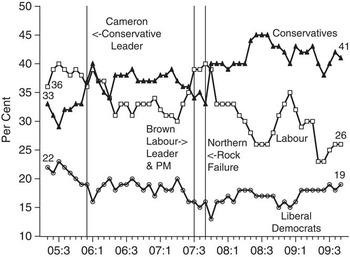
The Conservatives’ third consecutive loss in 2005 prompted considerable introspection in the party. The outcome was the selection of David Cameron as leader in December 2005. Cameron was young, moderate, ferociously supportive of the National Health Service (NHS), and a good performer both on television and in the House of Commons. He was determined to challenge Labour on the centre-ground of British politics. As Figure 1 shows, under Cameron's leadership, the Conservatives soon overtook Labour in the opinion polls. With the sole exception of a one-month blip occasioned by the fuel crisis of September 2000, this was the first time that the Conservatives had enjoyed a lead in the polls since the Exchange Rate Mechanism debacle of September 1992. From the autumn of 2007 onwards, Mr Cameron and his colleagues typically enjoyed a wide popularity edge over Labour, and Conservative performance in local council elections and by-elections improved commensurately.
Monthly poll of polls, voting intentions for Labour, Conservatives and Liberal Democrats, May 2005–September 2009 Note: Monthly averages of the commercial opinion polls reported in the UK Polling Report at ukpollingreport.co.uk/blog/voting-intention.

For its part, Labour pressed Tony Blair to act upon his promise, issued in advance of the 2005 election, to resign as prime minister at some opportune moment during his third term in office. He was duly replaced as leader in June 2007 by Chancellor of the Exchequer, Gordon Brown. Brown's ideological stance was virtually identical to Blair's. What Brown offered the party and the country was a solid reputation for competence in managing the economy, a quality that he obviously hoped to extend to other areas of government policy. During the summer of 2007, Brown's reputation as a ‘safe pair of hands’ helped Labour to re-establish a lead in the polls over the Conservatives. However, the ‘Brown bounce’ was short-lived. The collapse of the Northern Rock Building Society in September 2007 presaged the beginning of a serious credit crunch that by mid-2008 had developed into a full-blown recession. As Chancellor, Brown frequently claimed that he had ended the ‘boom and bust’ cycle that had plagued the British economy throughout much of the post-Second World War period. The financial crisis and deepening recession thus presented a serious challenge to his government's reputation for sound economic management. As Figure 1 indicates, Labour's poll ratings fell sharply after the Northern Rock failure, while those of the Conservatives and the Liberal Democrats recovered. Although all three major parties suffered modest popularity declines in the wake of the MPs’ expenses scandal in the summer of 2009, the Conservatives maintained a sizeable lead over Labour – averaging 12 per cent – throughout the period after the Northern Rock crisis.
In terms of illustrating the pressures placed by spatial and valence calculations on parties and voters, the Conservatives after their election defeat concluded that they had to move to the centre to attract more support. They duly moved closer to the median voter by electing a self-proclaimed moderate, David Cameron, as leader. Cameron quickly committed his party to protecting the NHS and maintaining strong public services. Labour under Blair already occupied the centre ground. The supposed attraction of Brown as his successor, as valence calculation implies, was that he would successfully deliver on a range of commonly agreed policy goals. For their part, the Conservatives under Cameron took every opportunity (and there were plenty after the Northern Rock collapse) to question Labour's competence – with some success, as the poll figures in Figure 1 suggest. In sum, between 2005 and 2009 Britain's two largest parties competed for popular support on both spatial and valence grounds, and their relative popularity ratings eventually were reversed. The period thus provides an excellent testing ground for studying the relative strengths of spatial and valence theories as explanations for changes in voter preferences.
Individual-level panel data are employed for this purpose. The data were collected in a six-wave national internet survey conducted in conjunction with the 2005 British Election Study (BES). The first wave went into the field in late March 2005, shortly before the general election was called. Wave Two, using a rolling design to capture opinion dynamics, was in the field throughout the campaign period. Wave Three was conducted in the week immediately after the election. Waves Four, Five and Six were carried out in May 2006, June 2008 and July 2009, respectively.
Extensive comparisons of variable distributions and competing models of electoral choice were conducted to assess the representativeness of the pre- and post-election panel waves of the internet surveys. These comparisons used data gathered in the traditional BES in-person pre-election and post-election probability survey. Analyses revealed that the internet and in-person survey samples were virtually and statistically indistinguishable.Footnote 20 In a vast majority of instances, model parameters calculated using the internet data were nearly identical to those generated using the in-person data.
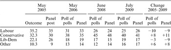
An analysis of the continuing representativeness of the post-election panel waves focused on vote and vote intention percentages recorded for the three main parties. The results are reported in Table 1. The table compares the vote shares for respondents who remained part of the panel through all six panel waves with the actual 2005 election result and the monthly average vote share recorded by UK Polling Report's ‘Poll of Polls’. Although there are some mild divergences from the actual result (for example, a four-point over-estimate of Liberal Democrat support among panel respondents in 2005), vote intentions reported by the panelists are very similar to those registered by the opinion poll averages. This level of similarity indicates that the sample of continuing BES panel respondents remained representative of the electorate's political preferences over the 2005–09 period.
Comparison of 2005–09 BES Panel's Party Vote Shares with the 2005 General Election Outcome and Subsequent Average Vote Intention Shares Reported in Monthly Public Opinion Polls

Note: Figures reported are column percentages. Poll of Polls is the monthly average of the commercial opinion polls reported in the UK Polling Report at ukpollingreport.co.uk/blog/voting-intention.
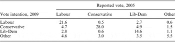
Individual-level changes in party preference among the panel respondents are displayed in Table 2. The table shows the turnover between reported vote in the May 2005 general election (Wave 3) and voting intention in July 2009 (Wave 6). In total, almost one person in three (32.5 per cent) reported a different party preference. In terms of specifics, the Conservatives garnered significant support from both Labour and the Liberal Democrats, making net gains of slightly over 4 percentage points from each of them. Sizeable gains also were made by several minor parties (British National Party (BNP), Greens, Plaid Cymru, Scottish National Party (SNP), United Kingdom Independence Party (UKIP)). Between 2005 and 2009, these parties collectively gained slightly over 11 per cent from the three major parties, while losing only just over 3 per cent.
Reported Vote in 2005 and Vote Intentions in 2009, 2005–09 BES Panel Respondents

Note: Percentages are calculated by dividing the number of respondents in each cell by the total number (N = 4,015) of 2005–09 panellists reporting a 2005 vote and a 2009 vote intention.
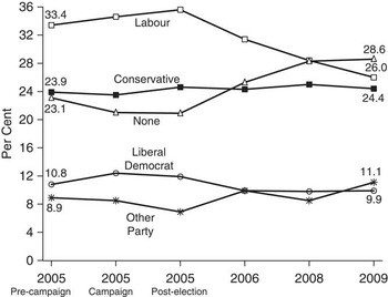
Figures 2–6 report changes in the three sets of explanatory variables that spatial and valence theories hold to be primarily responsible for (changes in) party choice. The number of time points varies across the figures because some questions were not asked in every survey wave. Figure 2 displays the aggregate-level and individual-level dynamics of party identification. As noted above, party identification is claimed as a signature variable by both spatial and valence theories. Accordingly, we treat it as a distinct explanatory factor. Figure 2a shows that identification with Labour fell substantially – from 33.4 to 26 per cent. In contrast, the percentage of Conservative identifiers in 2009 (24.5 per cent) was only slightly greater than it had been four years earlier (23.9 per cent), and still less than Labour's share. The proportion of Liberal Democrat identifiers remained more or less constant, oscillating around 10 per cent, a figure virtually identical to that which their predecessors, the Liberals, had recorded in the very first BES survey some four decades earlier.Footnote 21
Trends in Party Identification, March 2005–July 2009 BES Panel Question: ‘Generally speaking, do you think of yourself as Labour, Conservative, Liberal Democrat, (Scottish National in Scotland/Plaid Cymru in Wales) or what?’

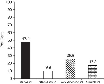
Another part of the party identification story is contained in Figure 2b, which summarizes individual-level dynamics across the multi-wave panel.Footnote 22 These data reveal that less than half of the 2005–09 panelists (47.4 per cent) were directionally stable identifiers. A further 9.9 per cent were stable non-identifiers. The large remaining group – over two-fifths of the panel – either moved between identification and non-identification one or more times (25.5 per cent) or actually switched parties once or more (17.2 per cent). As noted above, such sizeable individual-level dynamics are consistent with findings reported in recent research and with the running tally conception of partisanship articulated in valence politics theories of party support.
Individual-level dynamics in party identification, 2005–09 five-wave BES panel Note: 2005 campaign, 2005 post-election, 2006, 2008, 2009 panel waves.

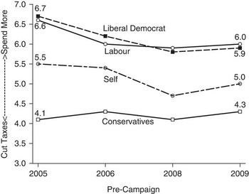
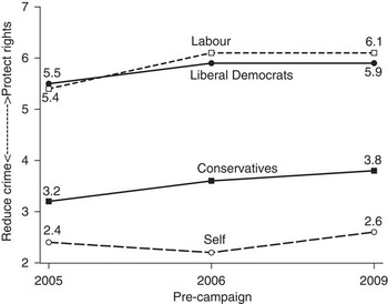
Figures 3 and 4 report changes in respondents’ self-placements and their placements of the main political parties on two eleven-point (0–10) ideological scales that previous research had shown to structure British political attitudes.Footnote 23 These are, first, a ‘cut taxes versus improve public services’ scale, which reflects general attitudes towards the size and function of the state and, secondly, a ‘punish criminals versus protect the rights of the accused’ scale, which taps preferences for authoritarian versus liberal approaches to maintaining social order while protecting human rights. Figure 3 illustrates how respondents shifted their positions on the tax/services scale. High values indicate a preference for more state activity; low values for less. From 2006 to 2009, on average, BES respondents’ perceptions both of their own positions and those of Labour and the Liberal Democrats moved slightly towards a preference for less state activity. Perceptions of the Conservatives moved marginally towards greater state activity. The average respondent also moved slightly closer to the average position assigned to the Conservatives. Similarly, small movements occurred for self-placements and party placements on the crime/rights scale (see Figure 4). Here, average self-locations became slightly less authoritarian, as did perceptions of the three main parties. In both 2005 and 2009, the average respondent clearly placed her/himself close to the ‘reduce crime’ end of the scale, and was considerably closer to the perceived position of the Conservatives than to either Labour or the Liberal Democrats.
Average positions on tax–spend scale, self-placement and placement of political parties, March 2005–July 2009 panel Question: ‘Now, another issue. Using the 0 to 10 scale on this card, where the end marked 0 means that government should cut taxes and spend much less on health and social services, and the end marked 10 means that government should raise taxes a lot and spend much more on health and social services, where would you place yourself on this scale? And where would you place … the Labour Party … the Conservative Party … the Liberal Democrat Party … ?’

Average positions on reduce crime–rights of accused scale, self-placement and placement of political parties, March 2005–July 2009 panel Question: ‘Some people think that reducing crime is more important than protecting the rights of people accused of committing crimes. Other people think that protecting the rights of accused people is more important than reducing crime. On the 0–10 scale, where would you place yourself on this scale? And where would you place … the Labour Party … the Conservative Party … the Liberal Democrat Party … ?’

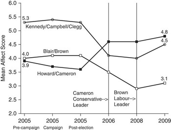
Figures 5 and 6 report the 2005–09 dynamics in two key valence politics variables – leader images and issue competence. The pattern of change in leader evaluations shown in Figure 5 indicates that from 2006 onwards the Conservative leader's ratings were running ahead of both the Liberal Democrats (who led in all three panel waves in 2005) and Labour (who also led the Conservatives in the three 2005 waves). Clearly, the Conservatives’ replacement of Howard by Cameron made a big difference. Equally clearly, after enjoying initial enthusiasm in the summer of 2007, Gordon Brown was considerably less warmly received than Tony Blair had been in 2005 and 2006 when the British public had become increasingly disillusioned over Britain's involvement in Iraq.Footnote 24 Circa 2009, Brown's average affect score was a dismal 3.1 points on the 0–10 ‘dislike–like’ scale. In fact, his score was lower than those recorded by former Conservative leaders William Hague and Michael Howard when they suffered serious electoral defeats in 2001 and 2005, respectively.
Average party leader affect ratings, March 2005–July 2009 BES panel Question: ‘Using a scale that runs from 0 to 10, where 0 means strongly dislike and 10 means strongly like, how do you feel about [name of party leader]?’

Party best able to handle most important issue, March 2005–July 2009 BES panel Question: ‘As far as you are concerned, what is the single most important issue facing the country at the present time? … Which party is best able to handle this issue?’

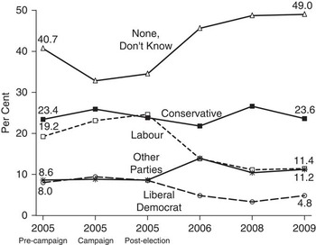
Figure 6 displays changes in judgements regarding the party best able to handle the most serious problem facing the country. As shown, large pluralities (ranging from 32.8 per cent in the run-up to the 2005 election to fully 49 per cent in 2009) stated either that there are no important issues or that no party is capable of handling them.Footnote 25 Figure 6 also shows that the Conservatives were slightly ahead of Labour in the run-up to the 2005 election, although Labour regained a minuscule lead at the time of that contest. Thereafter, the Conservatives moved well ahead, with the share of the electorate who thought Labour best on the most important issue falling from 24.6 in May 2005 to only 11.2 per cent in July 2009. The Liberal Democrats were consistently in poor shape. Only 8 per cent viewed them as best on the most important issue before the 2005 election, and four years later, merely 4.8 per cent did so.
To gauge the extent of individual-level change in perceptions of the party best on the most important issue, we construct a turnover table using the 2005 to 2009 post-election panel data. This analysis (not shown in tabular form) reveals that 29.2 per cent of the panelists maintained a consistent view of which party is most competent on their key issue. An additional 26 per cent consistently reported that no party was best, that they did not know which party was best, or that there was no important issue. Most of the large group (44.8 per cent) indicating instability in their party-issue performance judgements moved between choosing and not choosing a party (33.4 per cent), with a smaller number migrating between parties (11.4 per cent). Competence judgements on salient issues thus exhibited levels of mutability consonant with the aggregate and individual dynamics in party support discussed above.
In sum, the data reported in this section lend a priori credence to the claims of party identification, spatial position and valence judgements as explanatory factors in the evolution of party support. Partisanship manifested clear aggregate-level and individual-level dynamics, with the Conservatives improving their position relative to their competitors, but failing (just barely) to overtake Labour. In terms of spatial positions, the average voter saw her/himself as drawing closer to the Conservatives on the tax/spend scale, while remaining much closer to that party than to its rivals on the crime/rights scale. For the key valence variables of leader images and party competence, dynamism was the watchword, with the patterns of movement placing the Conservatives well ahead of their rivals. In the next section, we develop a series of individual-level models to gauge the impact of these several predictor variables on the dynamics of party support.
Model specification
To assess the claims of rival spatial and valence theories as explanations of the dynamics of party support, we use the maximum number of observations permitted by the available panel data. Since the spatial measures described in the previous section were collected only in a limited number of waves, this means that models incorporating the tax/services scale (measured in Waves 1, 4, 5 and 6) can be estimated using four effective panel waves; those incorporating the crime/rights scale (measured in Waves 1, 4 and 6) are estimated using three waves.Footnote 26 Since we are interested in the dynamics of party preference, we follow Finkel and employ lagged endogenous variable models, measuring all predictor variables in levels.Footnote 27 The inclusion of a lagged endogenous variable on the right-hand side of each model means that the reported coefficients on each predictor variable effectively measure the time t effects of that variable on partial changes in the dependent variable.Footnote 28
To compare the effects of spatial calculations and valence judgments on party support, we follow standard practice and employ statistical controls for a range of other variables that might influence vote choice. Consonant with recent research,Footnote 29 since Labour is the incumbent party throughout the 2005–09 period, the first model in each set is a binomial logit of Labour versus all other parties voting.Footnote 30 This model investigates the basic decision whether to (continue to) support the governing party. The second model is a multinomial logit specification of intending to vote for various opposition parties (Conservative, Liberal Democrat, other parties), with Labour support as the reference category. This model assesses which factors are important for prompting voters to opt for various opposition parties.
Our modelling strategy begins with a baseline specification that involves only a lagged endogenous variable:


We then add a series of predictor variables that capture various influences on party support. The first set of predictors includes standard demographic controls – age, gender, education, trade union membership, social class and home ownership – all measured in the first panel wave. The second set of predictors, also measured in wave one, includes controls for newspaper readership (dummy variables for readership of major national daily newspapers), and for views (positive or negative on a five-point scale) of Britain's involvement in the war in Iraq. The predictors in the third set are measures of party identification. We construct dummy variables for identification with Labour, Conservative, Liberal Democrat and various other parties, with each of these variables weighted by strength of identification on a 1–3 scale.Footnote 31
The fourth set of predictors taps spatial proximities. As anticipated above, we use two different spatial measures – one for tax–services and one for crime–rights. Since the crime–rights scale is available for fewer time points than the tax–services scale, we estimate two different versions of the spatial model – one that includes tax–services only and one that includes both tax–services and crime–rights.Footnote 32 The fifth set of predictors assesses valence judgements about the three major parties. The variables are affect for each of the three major party leaders; assessments of parties’ policy competence in four major issue areas;Footnote 33 and judgements regarding which party is best able to deal with the most important problem facing Britain today.Footnote 34
Finally, we specify a composite model that allows us to evaluate the explanatory power of the various sets of predictor variables. For example, the composite model for Labour versus all other party voting is:

where ‘leader images’ are affect scores on 0–10 scales, ‘party best’ is the party deemed best able to deal with the most important issue facing Britain; ‘party competence’ refers to the party's ability to handle policy on the economy, the NHS, crime and terrorism, and ‘newspapers’ is a series of dummy variables tapping newspaper readership patterns. An equivalent multinomial logit model is employed to study opposition party voting.
Spatial calculations and valence judgements
In this article, a key claim is that, in a direct comparison, valence judgements can, and do, substantially outperform spatial calculations in explaining vote choice. However, we also acknowledge that valence judgements may be influenced by spatial considerations further back in the funnel of causality. The idea is that voters’ ideal points on classic spatial issues such as tax–spend and crime–rights tradeoffs and, a fortiori, on a more general ideological continuum, such as the left–right dimension, are conditioned by basic value orientations that are reflected in distances between those ideal points and perceived party locations. Regarding the latter, the ‘issue ownership’ literature has long maintained that perceived party locations reflect not only parties’ current attempts to position themselves advantageously, but also the historically conditioned images that particular parties develop as advocates and administrators in different policy domains.Footnote 35 The end result is that, at any time t, perceived distances between parties and voters provide the latter with helpful cues for assessing how competing parties will handle salient issues. As argued above, these issues typically have valence properties.
After performing possibly ‘rough and ready’ spatial calculations, voters sensibly economize by using them as heuristic devices when assessing the performance of competing parties. For example, a voter who considers that party X is distant from her/his own spatial position will conclude that X is unable or unwilling to design and implement policies that will further the achievement of valence politics goals of interest. The very extremity of X's position cues the voter that X is unlikely to provide effective policy delivery for the valence issues that matter for that voter. By the same token, the closer party X is to a voter's ideal point, the more likely the voter is to conclude that X will deliver effective policies on those issues. These cueing properties of spatial calculations have the potential to make them important sources of valence judgements.
We investigate this conjecture by developing a set of valence models, one for each of the three major parties. This requires, first, that we construct a single valence index for each party based on the various valence indicators that are used in Equation 2 above. The valence indices for Labour and the Conservatives combine party leader evaluations, assessments of the party best able to deal with the most important problem facing the country, and evaluations of the prospective policy competence of a party with regard to the economy, the NHS, crime and terrorism. Since the BES panel surveys did not ask questions about likely Liberal Democrat policy performance, the valence index for the Liberal Democrats is based on leader evaluations and best party only.Footnote 36
When assessing the effects of spatial calculation in these analyses, we specify models that, with the obvious exception of the spatial terms themselves, exclude the independent variables employed in our vote equations. This enables us to use these same valence equations when, as discussed below, we test for the weak exogeneity of valence with respect to the vote. In the models of Labour, Conservative and Liberal Democrat valence assessments, we use six exogenous instrumental variables. The first of these is a measure of economic evaluations which combines prospective and retrospective judgements of the economy at the personal and national levels. Previous research has demonstrated that these evaluations have powerful impacts on assessments of the prospective managerial capabilities of the major parties.Footnote 37 Our expectation is that evaluations will be positively associated with valence judgements of the incumbent party and negatively associated with those of the opposition parties. To complement these cognitive evaluations of the economy, we also include a variable that reflects strong negative emotions towards the economy – a measure of whether respondents felt angry about recent economic developments. Since this variable expresses negative emotions, the expectation is that the signs on the coefficients will be the opposite of those for economic evaluations.
The third, fourth and fifth instruments are measures of trust in each of the three major parties.Footnote 38 The expectation is that valence judgements about each party should be positively associated with the level of trust in that party. Finally, we include a measure of attitudes towards the European Union (EU). The expectation here is that pro-EU attitudes will be positively associated with valence judgements about pro-EU parties (Labour and the Liberal Democrats) and negatively associated with valence judgements about broadly Eurosceptic parties (here, the Conservatives).Footnote 39 Other elements in the valence model are the six spatial proximity variables employed in Equation 2. The resulting model of valence judgments for party X is:

Exogeneity Tests
In suggesting that valence judgements are determined in part by spatial proximities, whereas valence judgements have a powerful impact on vote, we propose the existence of a recursive causal chain in which: (1) proximities affect valence judgements and (2) valence judgements affect vote. This claim requires us to address the question of possible simultaneity biases and attendant model mis-specification. To justify estimating parameters in a model for (1), we need to demonstrate the weak exogeneity of spatial proximities to valence judgements.Footnote 40 To justify (2), we similarly need to demonstrate the weak exogeneity of valence judgements with respect to the vote. We provide these justifications by conducting Hausman tests.Footnote 41 These tests involve estimating equations for each putative weakly exogenous variable using appropriate instrumental variables. Results are reported in Appendix 1. They clearly support the inferences that issue proximities are weakly exogenous to valence judgements and valence judgements are weakly exogenous to vote. These results imply that the model specifications presented in Equations 2 and 3 can be estimated without risking simultaneity bias.
Empirical results
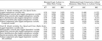
Table 3 provides summary statistics for a range of rival models of vote choice. Recall that tax–spend spatial scales are available for four data waves and crime/rights scales are available for three waves. The table accordingly differentiates between models that include only tax–services (Panel A, N = 6,768) and those that include both tax–services and crime–rights (Panel B, N = 4,260).Footnote 42 Model 1 in each panel includes only a single lagged endogenous variable, as in Equation 1a, or multiple lagged endogenous variables, as in Equation 1b. Model 2 in each panel includes the relevant lagged endogenous variables together with demographic controls (age, gender, education, trade-union membership, social class and home ownership). Model 3 includes a further set of controls for newspaper readership and attitudes towards the Iraq War. Similarly, Model 4 focuses on partisanship; Model 5 on spatial proximities; and Model 6 on valence considerations. Model 7 is a composite that includes all of the independent variables, as in Equation 3. As noted above, the Labour voting models are estimated using binomial logit. Models for choices among opposition parties are estimated using multinomial logit with Labour as the reference category.
Summary Statistics for Rival Vote Intention Models

Notes: Panel A: Models including only Tax–Spend Scales: N = 6,768; Clusters (individuals), 2,711. Panel B: Models including Tax–Spend and Crime–Rights Scales: N = 4,260; Clusters (individuals), 2,351. *McFadden R 2.
The three sets of summary fit statistics displayed in Table 3 all point to the same conclusions. Recalling that lower AIC and BIC statistics indicate superior model fit,Footnote 43 it is clear that Models 2 to 7 offer improvements over the Model 1 baseline. But the extent of improvement varies widely. For example, the improvement afforded by demographics (Model 2) is extremely modest – a mere 0.01 improvement in the McFadden R 2 and very small reductions in AIC and BIC. The newspaper readership/Iraq War control model (Model 3) does not fare much better. In contrast, the spatial proximities model (Model 5) exhibits considerably more explanatory power (e.g., the McFadden R 2 rises to 0.48 in the Panel B model for Labour, with commensurate reductions in AIC and BIC). Yet the spatial models do not perform as well as either the pure party identification models (Model 4) or the valence models (Model 6). Indeed, the statistics summarized in Table 3 testify that the valence model clearly outperforms all of its rivals, consistently exhibiting the highest pseudo R 2 values and lowest AIC/BIC scores.
However, there is more to the story. Table 3 shows that the composite model (Model 7) which includes variables from each of the rival models outperforms any of the individual rivals. The McFadden R 2 values for the composite model are typically 6 to 9 points greater than the best individual model, again with correspondingly lower AIC and BIC scores. This result indicates that there is potentially a role in the determination of vote choice for any or all of the different explanatory factors identified in Equation 3. To evaluate the relative importance of the different factors, it is necessary to go beyond overall model fit statistics to consider the impact of individual predictor variables.
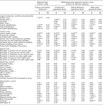
Table 4 reports the results of estimating Equation 2 for both Labour voting (Panel A) and for the choice among opposition parties (Panel B). The estimation procedure clusters the data by individual panel respondent and provides robust standard errors. Note that because of the inclusion of various lags in the models, the effective number of cases is 4,260, representing some 2,351 individuals. Models that exclude the crime–rights variables (available for only three data waves) yield more effective cases without substantially affecting any of the reported coefficients.Footnote 44
Binomial and Multinomial Logit Vote Intention Models

*p ≤ 0.05; **p ≤ 0.01; ***p ≤ 0.001.
Note: Reference category for occupational class is never worked/other. N = 4,260; clusters (individuals) = 2,351; robust standard errors reported.
The statistics in Table 4 adjudicate the competing claims of the rival theories of voter choice. Consider the coefficients and standard errors reported in Panel A, which concerns determinants of Labour vote choice. Bearing in mind that including a lagged dependent variable means that the model effectively explains partial changes in Labour support from time t−1 to time t, several conclusions are apparent. First, all of the coefficients for the lagged endogenous variable and the partisanship terms are significant and in the predicted direction: positive in the case of Labour vote at t−1 and Labour partisanship; and negative in the case of Conservative and Liberal Democrat partisanship. Secondly, most coefficients for the two sets of control variables are not statistically significant (p ≤ 0.05). None of the newspaper readership variables achieves significance, implying that changes in Labour voting intentions after 2005 owed little or nothing to exposure to information in particular newspapers. The Iraq War control term is positive (approval of the war disposed people to shift towards Labour), although not quite significant at conventional levels.
Regarding demographic controls, older people tended to move away from Labour more than did their younger counterparts (i.e., the age coefficient is significant and negative, b = −0.02). Three of the occupational class variables also produced small negative effects: compared with the base class category (‘never worked’), professional/managerial, clerical/sales and manual workers tended to move away from Labour after 2005. However, it bears emphasis that these effects are very modest in their substantive implications. Recall from Table 3 that demographic factors added little explanatory power to the baseline lagged endogenous variable model, the increase in R 2 being only 0.01.
The most important findings in Panel A concern the valence and spatial variables. Three of the six spatial variables in Panel A exhibit significant effects. Proximity to Labour on the tax/services scale correctly produces a significant positive effect (b = 0.15), whereas proximity to the Conservatives has the anticipated negative effect (b = −0.08). However, the third significant spatial coefficient – proximity to the Conservatives on crime–rights – is incorrectly signed. The positive coefficient (b = 0.10) counter-intuitively suggests that, as people drew close to the Conservatives on crime–rights, the more likely they were to support Labour. Neither of the spatial variables for the Liberal Democrats approaches significance.
The performance of valence variables in the Labour model is quite straightforward. Although a small number of these variables fail to achieve statistical significance, all are correctly signed – the signs for all the Labour valence variables are positive and all of those for the Conservative and Liberal Democrat terms are negative. The Labour leadership coefficient is sizeable, significant and positive (b = 0.24), suggesting that an important reason for the decline in Labour's support since 2005 involved the declining ratings of party leaders Blair and Brown. As also expected, the Liberal Democrat leadership coefficient is significant and negative (b = −0.12).
Regarding party performance on important issues, the effect of the ‘Labour best’ variable on voting for that party is predictably positive and significant (b = 1.05) and that for Liberal Democrats is negative and significant (b = −0.85). The effect of Conservative valence judgements on Labour voting appears to operate through the overall policy competence measure. As expected, the effect of Labour policy competence is positive and significant (b = 0.73), but there is also a significant negative effect produced by Conservative policy competence (b = −0.31). Taken together, these findings suggest that the decline in Labour support after 2005 was partly a function of growing perceptions that the party had faltered, especially on the economy, but also partly a result of the Conservatives’ ability to convince some voters that the party could perform soundly in key policy areas.
Panel B of Table 4 tells a similar story to Panel A. Most of the media and demographic control variables for the Conservatives, Liberal Democrats and other parties are not significant, although there are a few exceptions. Party identification coefficients are generally significant and are correctly signed. For example, for Conservative voting, Conservative partisanship is positively signed, Labour partisanship is negatively signed and Liberal Democrat partisanship is correctly signed but not significant. And, similar to Panel A of this table, the spatial coefficients present a somewhat inconsistent picture. For Conservative voting, the Labour and Conservative tax–services variables are significant and correctly signed (negative and positive, respectively). None of the other four variables has a significant effect. For Liberal Democrat voting, three of the six spatial terms are significant and correctly signed, although one (for Conservative policy competence) is significant and perversely signed. Regarding voting for other parties, only the Labour tax–services coefficient is significant and correctly (negatively) signed.
Once more, most coefficients for the valence variables are consistent with expectations. Of the eight valence coefficients for Conservative voting, six are significant and correctly signed. For Liberal Democrat voting, five coefficients are significant and correctly signed. Finally, four of the valence coefficients for other party voting are significant and all are correctly signed.
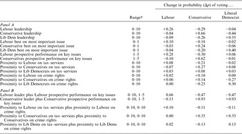
Since logit coefficients are not easily interpreted,Footnote 45 we compute changes in the probability of voting for various parties when each of the spatial and valence predictor variables is moved from its minimum to its maximum value, holding all other variables constant at their means.Footnote 46 The largest changes in probabilities (Δp values) are those associated with the valence variables (see Table 5, Panel A). None of the spatial proximities produces a change in probability of voting for any of the parties greater than 0.30, and only four of the eighteen changes are greater than 0.20. In contrast, half of the Δp values for the valence variables are greater than 0.20, and six of them exceed 0.40. For Conservative voting, a shift from 0 to10 on the party's leader scale increases the probability of voting for the party by 0.66. Similarly, an increase from 1 to 5 on the Conservative policy competence scale engenders a 0.62 increase in the probability of voting for the party.
Changes in Vote Intention Probabilities Associated With Various Predictor Variables

† Range: change in each of the predictor variables used for calculating changes in vote probabilities.
Panel B of Table 5 illustrates changes in vote probabilities associated with combinations of changes in valence and spatial measures. Here the difference between valence and spatial effects is even more pronounced. For example, a change in both Conservative leader evaluations and Conservative policy competence judgements from their minimum to their maximum values increases the probability of switching to the Conservatives by fully 0.93. This is almost three times the size of the largest spatial combination (0.35) for the combination of changes in Conservative tax–service proximity and Conservative crime–rights proximity. These differences in changes in probability values testify to the dominance of valence judgements over spatial proximities as direct determinants of vote choice.
Indirect Effects
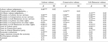
As hypothesized above, spatial considerations may have additional, indirect effects on the vote by virtue of their influence on valence judgements. Table 6 reports the results of estimating Equation 3 for each of the three main parties. Since the dependent variables are all 0–10 scales, estimation is by Ordinary Least Squares regression, with robust standard errors being calculated since the data are clustered by respondent. The models are reasonably well determined, with R 2 values ranging from 0.32 for Liberal Democrat valence judgements to 0.66 for Conservative valence judgements and 0.71 for Labour ones.Footnote 47 The values of the spatial coefficients offer strong support for the hypothesized spatial calculation-to-valence judgements causal linkage. In the three models, all coefficients are correctly signed, and seventeen out of twenty-one are statistically significant. In every case, the proximity terms for the party whose support is being analysed have positive coefficients while the proximity terms for the competing parties have negative ones. For example, in the Labour model, both Labour spatial variables – tax–services and crime–rights – have positive coefficients, whereas the comparable coefficients for Conservative and Liberal Democrat voting are negative. And, as just noted, a large majority of these coefficients are statistically significant (p < 0.001 in all cases). All spatial coefficients are significant in the Labour model; four out of six are significant in the Conservative model; and five out of six in the Liberal Democrat one. There is a clear contrast between this strong and consistent pattern for spatial effects on valence judgements in Table 6, and the weaker, more variable direct effects of spatial variables on voting intentions (see Tables 4 and 5). This contrast lends additional credence to the conjecture that a hitherto neglected component of the influence of spatial calculations on voting behaviour is indirect, operating through valence judgements.
The Impact of Spatial Proximities on Labour, Conservative and Liberal Democrat Valence Judgements

*p ≤ 0.05; **p ≤ 0.01; ***p ≤ 0.001.
Note: N = 4,612, clusters = 2,979; robust standard errors reported.
Summary and conclusion: Downs and Stokes reconsidered
Recent studies of voting behaviour in Britain, Canada and the United States have demonstrated that valence models outperform spatial rivals in analyses of electoral choice. To the extent that these studies have considered individual-level changes in party support, they have focused heavily on the official ‘short’ campaign periods preceding general elections. In this article, we have extended this line of research by investigating the dynamics of party support in the British case over the ‘long campaign’ period between 2005 and 2009. Newly available BES multi-wave panel data reveal that the valence politics model outperforms its spatial competitor in terms of direct effects on changes in vote intentions over this four-year period. However, spatial effects do not disappear when valence considerations are controlled – a composite model that includes both types of variables has the strongest explanatory power.
Another important finding is that spatial calculations act as a source of valence judgements. The hypothesis considered is that Downs undergirds Stokes – voters use spatial calculations as heuristic devices when assessing party competence. Parties viewed as closer than their competitors to voters in spatial terms are more likely to be judged as credible vehicles for achieving widely shared policy goals such as economic prosperity, health care and public safety. Analyses are consistent with this spatial cueing hypothesis. Tests for the weak exogeneity of spatial calculations with respect to valence judgements, and of valence judgements with respect to vote intentions, lend confidence that the results are not statistical artefacts.
These findings have significant substantive implications, suggesting that the dynamics of British party support after 2005 can be understood in terms of the interplay of valence and positional politics. One important consideration is that Labour lost its leadership advantage over the Conservatives. After an initial burst of enthusiasm, voters quickly soured on Blair's successor, Gordon Brown. In contrast, although new Conservative leader, David Cameron was not greeted with great warmth, he ran well ahead of his predecessor, Michael Howard, and, more importantly, well ahead of Brown. With Cameron at the helm, the leadership heuristic was no longer a barrier to his party's electoral success. The Conservatives also managed to reinvigorate their reputation for managerial competence and, although their share of partisans increased only very slightly in absolute terms, Labour's cohort of identifiers dropped by nearly 10 per cent. Consistent with the valence politics model's claim that party identification has dynamic properties, over two-fifths of the BES panellists reported changing their partisanship one or more times between 2005 and 2009.
Finally, there were forces at work consistent with the spatial cueing hypothesis. The Conservatives’ move towards the political centre under Cameron, in conjunction with moves by voters on the tax–spend scale that worked to reduce their distance from his party, played an indirect role in restoring his party's electoral fortunes. This shift to the centre helped persuade voters that the Conservatives could deal competently with challenges concerning the economy, public services and public safety. In turn, these valence judgements about prospective policy performance were a motor of increasing Conservative support.
In conclusion, the major message of this article is that both spatial and valence considerations have consequential effects on electoral choice. Spatial variables have both direct and indirect effects on the vote, but their direct effects are substantially weaker than those of their valence rivals. Thus, it is not surprising that the core terrain on which parties typically fight general elections involves valence judgements. A party's best interests lie in convincing the electorate of its competence in the three key policy areas of the economy, public services and public safety – and in contriving to tarnish the corresponding competence images of competing parties. Valence politics is not the exclusive preserve of the British voter. Rather, as recent studies in Canada and the United States underscore, valence considerations powerfully influence electoral choice in other mature democracies. What is less well understood is the relationship between valence judgements and spatial calculations and, in particular, whether there are cueing effects of the latter on the former, such as those operating in the British case. In the years ahead, the growing availability of high quality multi-wave panel data in a variety of countries should enable researchers to pursue these theoretically interesting topics central to understanding the dynamics of party support in broader comparative perspective.
Appendix 1: Exogeneity tests
Hausman tests for (weak) exogeneity involve the use of two equations – one for the dependent variable itself and one for the explanatory variable that is hypothesized to be weakly exogenous to the dependent variable.Footnote 48 The test requires that the equation for the predictor variable contains at least one instrumental variable that is not included in the equation for the dependent variable. In our case, we have several such instruments in each of our Hausman tests.
Our models of the vote intention–valence judgement relationship are:


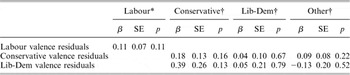
The test consists in regressing vote intentions on all the exogenous variables in both equations. Residuals from this regression are then added to the vote-intention equations reported in Table 4. If these residuals yield non-significant coefficients, then we conclude that the valence measures are weakly exogenous to vote intentions. The intuition here is that if the unexplained variance in valence is unrelated to vote intentions (which it must be if the residual terms are non-significant), then estimates of the impact of valence in the vote intention equation do not suffer from simultaneity bias.
Table A1 reports results. Parameters in the Labour vote intentions are estimated by binomial logistical regression, and the choice among opposition parties (Conservative, Liberal Democrat, other party voting, with Labour voting as the reference category), by multinomial logistic regression. Residuals from the Labour valence-judgements equation are added to the Labour equation only. Since there is no valence term for ‘other’ parties, in the multinomial logit only residuals from the Conservative and Liberal Democrat valence equation are added. As the table indicates, all the residual terms in both equations are non-significant. This result indicates that valence calculations are weakly exogenous to vote.
Hausman Test Results: Effects of Labour, Conservative and Liberal Democrat Valence Judgement Residuals in Logit and Multinomial Vote Intention Models

* Labour – not binomial model. † Opposition – multinomial logit model (base category is Labour).
The Hausman tests for the exogeneity of spatial proximities to valence are slightly more complicated than those presented in Table A1. This is because we need to specify equations for proximities on both tax–services and crime–rights. The instruments that we use in the tax–services equations are the respondents’ family income, her/his sense that s/he is treated fairly by government and her/his sense of relative deprivation.Footnote 49 The model for tax–services proximities is:

In the crime–rights models, we add further instruments of attention to politics, personal political efficacy and sense of civic duty.Footnote 50 This gives:

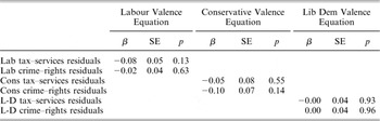
The valence model is the same as that given in Equation A2. The Hausman tests for spatial proximity exogeneity consist in (a) regressing tax–services proximities for party X on all the exogenous variables in Equations A2 and A3 and holding the residuals in XResTax; (b) regressing crime–rights proximities for party X on all the exogenous variables in Equations A2 and A4 and holding the residuals in XResCrime; (c) estimating Equation A2 with the addition of XResTax and XResCrime as predictors. Again, if the residual terms are non-significant at stage (c), then spatial proximities are weakly exogenous to valence and we are justified in estimating Equation A2.
Table A2 reports significance levels of the relevant residual terms in the Labour, Conservative and Liberal Democrat models. As the results indicate, all predictors are non-significant in all models, strongly supporting the notion that spatial calculation is weakly exogenous to valence judgements.
Hausman Test Results: Effects of Tax–Services and Crime–Rights Residuals in Labour, Conservative and Liberal Democrat Valence Judgement Models