1 Introduction
Inspired by aspects of the runout of granular materials such as ice from glacier calving, debris from landslides, dredged materials, industrial wastes, volcanic ash and snow-laden air and similar phenomena, we study the flow of granular material along the upper surface of a liquid. Key open questions include the generation of tsunami waves once the granular materials hit the surface of an ocean, lake or river, and how the granular materials spread after the initial impact. Here we address the latter and investigate the case of the flow of buoyant granular material in a channel containing liquid of a greater density, so that the granular material floats near the air–liquid interface. Such flows have only been considered for simple fluids, for example, in the viscous limit in the context of oil spreading in the sea, and ice shelf and grounding line dynamics (see, e.g. Hoult Reference Hoult1972; Lister & Kerr Reference Lister and Kerr1989; Pegler & Worster Reference Pegler and Worster2013). Similar phenomena also appear in freshwater rivers flowing into salt water oceans and intrusive gravity currents entering stratified environments (see, e.g. Holyer & Huppert Reference Holyer and Huppert1980; de Rooij, Linden & Dalziel Reference de Rooij, Linden and Dalziel1999; Maurer, Bolster & Linden Reference Maurer, Bolster and Linden2010; Carazzo & Jellinek Reference Carazzo and Jellinek2012).
Related previous studies on this topic also include the collapse of heavy beads along an inclined substrate into a shallow layer of water, inspired by landslide processes (see, e.g. Viroulet, Sauret & Kimmoun Reference Viroulet, Sauret and Kimmoun2014; Zitti et al. Reference Zitti, Ancey, Postacchini and Brocchini2016). The major focus of Viroulet et al. (Reference Viroulet, Sauret and Kimmoun2014) and Zitti et al. (Reference Zitti, Ancey, Postacchini and Brocchini2016) is on the generation of tsunami waves caused by the impact of the granular material on the shallow water. The spreading of heavier granular materials into a water-filled channel has also been investigated through a series of experiments with different initial conditions and granular materials (Hallworth & Huppert Reference Hallworth and Huppert1998; Pailha, Nicolas & Pouliquen Reference Pailha, Nicolas and Pouliquen2008; Rondon, Pouliquen & Aussillous Reference Rondon, Pouliquen and Aussillous2011) and through theoretical models (see, e.g. Pailha & Pouliquen Reference Pailha and Pouliquen2009) and numerical simulations (Topin et al. Reference Topin, Monerie, Perales and Radjai2012). Similar to the situation of dry granular spreading, investigated experimentally (Lube et al. Reference Lube, Huppert, Sparks and Hallworth2004, Reference Lube, Huppert, Sparks and Freundt2005; Balmforth & Kerswell Reference Balmforth and Kerswell2005; Thompson & Huppert Reference Thompson and Huppert2007) and theoretically (Savage & Hutter Reference Savage and Hutter1989; Pouliquen & Hutter Reference Pouliquen and Hutter2002; Staron & Hinch Reference Staron and Hinch2005; Larrieu, Staron & Hinch Reference Larrieu, Staron and Hinch2006; Staron & Hinch Reference Staron and Hinch2007), in experiments of granular collapse within a liquid of lower density, a final profile shape was observed at late times with a finite runout distance of the granular material. However, when the viscosity of the ambient liquid becomes important, the dynamics of granular collapse is modified from the case of dry granular collapse (du Pont et al. Reference du Pont, Gondret, Perrin and Rabaud2003; Pailha & Pouliquen Reference Pailha and Pouliquen2009; Topin et al. Reference Topin, Monerie, Perales and Radjai2012).
Another related topic concerns particle-laden gravity currents driven by the density difference between the particles and the ambient liquid (see, e.g. Bonnecaze, Huppert & Lister Reference Bonnecaze, Huppert and Lister1993; Bonnecaze et al. Reference Bonnecaze, Hallworth, Huppert and Lister1995). In these flows there is also a finite runout distance, because the heavy particles settle out from the current so that the bulk density difference eventually becomes zero and the current stops. The speed of particle sedimentation is typically determined by a balance between the gravitational force and viscous drag (Bonnecaze et al. Reference Bonnecaze, Huppert and Lister1993). We also note that the particle concentrations in these particle-laden flows are typically much lower than the particle concentrations in the granular collapse experiments of Hallworth & Huppert (Reference Hallworth and Huppert1998) and the granular intrusion experiments described in the current work.
In this study we focus on the temporal evolution of relatively light beads spreading from a lock into a relatively denser ambient liquid. We describe a series of experiments of granular intrusions into a water tank in § 2. We interpret the major observations on the time-dependent profile shape, front location and runout distance in § 3. We also provide scaling arguments to rescale and collapse the experimental data into universal curves, which capture the major physics during the spreading process. We summarize the major findings in § 4, and comment on open questions and future directions and the major differences between the interfacial granular intrusion and three other related problems: the intrusive gravity current, the particle-laden gravity current and the dry granular collapse problems.
2 Experimental design
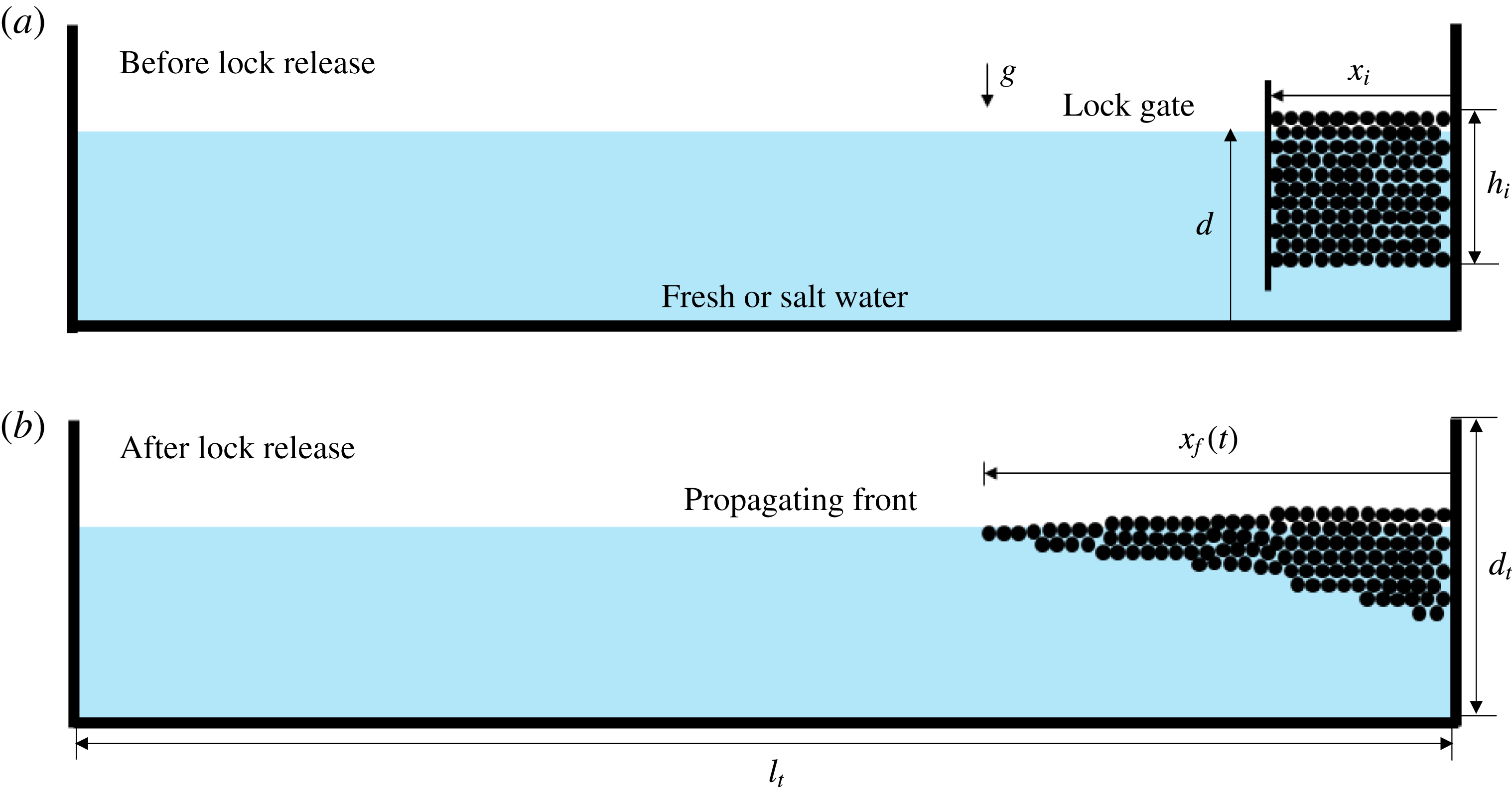
We examine the spreading of a constant volume of buoyant particles, floating on a liquid of relatively greater density. The experiments were conducted in a rectangular tank of length
 $l_{t}=2.09\pm 0.01$
m, width
 $w_{t}=0.15\pm 0.01$
m and depth
 $d_{t}=0.57\pm 0.01$
m, as sketched in figure 1. Before each experiment, the tank was filled with either fresh water, density
 $\unicode[STIX]{x1D70C}_{w}=998~\text{kg}~\text{m}^{-3}$
, or saturated sodium chloride solution, density
 $\unicode[STIX]{x1D70C}_{sw}=1180~~\text{kg}~\text{m}^{-3}$
. The water depth
 $d$
was set to
 $d=15$
or 20 cm. A lock gate of small thickness (2.5 mm) was placed at a location
 $x_{i}$
(i.e. the lock length), measured from one end of the tank (i.e. from the origin at
 $x=0$
), as shown in figure 1(a). The gap between the lock gate and the origin was filled with a mass
 $m$
of spherical polypropylene beads (McMaster Carr, 1974K2) of radius
 $r=1.6$
mm and density
 $\unicode[STIX]{x1D70C}_{b}=910~\text{kg}~\text{m}^{-3}$
. The beads were carefully maintained in an initial rectangular shape before the removal of the lock gate (figure 1
a).
To start the experiments, we quickly (within 0.1 s) lifted the lock gate vertically and the beads spread horizontally along the surface of the liquid (figure 1
b). A digital camera was used to take videos from either the side or above the tank. Digiflow software (Dalziel Reference Dalziel2005) and MATLAB image processing toolbox were used to analyse videos and extract the interface shape between the beads and water and the location of the front of the current of beads. In order to explore buoyancy effects, we used either fresh water or saturated salt water as the ambient liquid in the tank. We also varied the depth
 $d$
of the liquid and the total mass of beads
 $m$
. In addition, to explore the influence of the initial aspect ratio of the beads, we kept the mass of beads
 $m$
constant but varied the initial lock length
 $x_{i}$
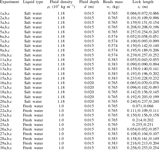
. The experimental parameters are given in table 3 and the results are summarized in table 4 in appendix A. The error estimates on the measured parameters in table 3 and thereafter come from the standard deviation of repeated experiments.
Sketch of the experimental set-up (a) before and (b) after release of the lock gate. The lock length is denoted by
 $x_{i}$
, while the front location is denoted by
 $x_{f}(t)$
.

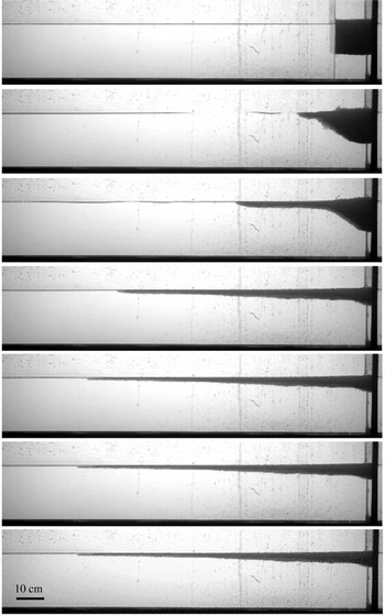
Side views of the spreading beads in a representative experiment (experiment 2a in table 3). The pictures were taken at
 $t=\{0,0.6,1.8,6.0,10,20,30\}$
s. The tank was filled with saturated salt water of depth
 $d=15\pm 0.1$
cm,
 $m=765\pm 1$
g and
 $x_{i}=10$
cm. The pictures show the initial spreading with time followed by the front coming to a halt.

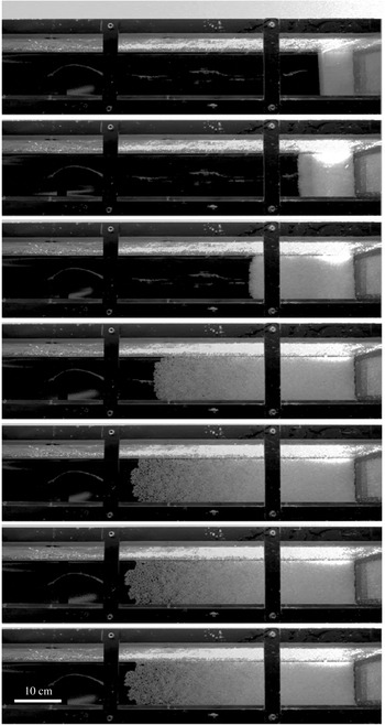
Top view of the spreading beads in a representative experiment. The propagating front remains almost uniform across the width of the tank until the current is close to its final length. The pictures were taken at
 $t=\{0,0.6,1.8,6.0,10,20,30\}$
s. The experimental parameters are the same as the experiment in figure 2.

3 Experimental results
3.1 Interface shape
Side and top views of two representative experiments are shown in figures 2 and 3. In these two experiments with identical parameters, the tank was filled with saturated salt water of depth
 $d=15\pm 0.1$
cm, the lock length was
 $x_{i}=10$
cm and the total mass of the beads was
 $m=765\pm 1$
g.
For small initial lock lengths (e.g.
 $x_{i}\leqslant 10$
cm), the interface shape exhibits an almost constant slope near the origin between
 $t=0.6$
s and
 $t=2.2$
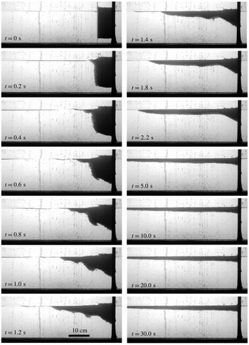
s before decreasing to a smaller angle at the end. Shear-driven instabilities also appear at the interface at the beginning of the experiments. This experiment (not included in table 3) was conducted using saturated salt water of depth
 $d=15\pm 0.1$
cm,
 $m=765\pm 1$
g and
 $x_{i}=5$
cm.

For large initial lock lengths (e.g.
 $x_{i}\geqslant 20$
cm), there exists a ‘frozen’ region near the origin where the interface shape stays unchanged. This experiment (not included in table 3) was conducted using saturated salt water of depth
 $d=15\pm 0.1$
cm,
 $m=765\pm 1$
g and
 $x_{i}=25$
cm.

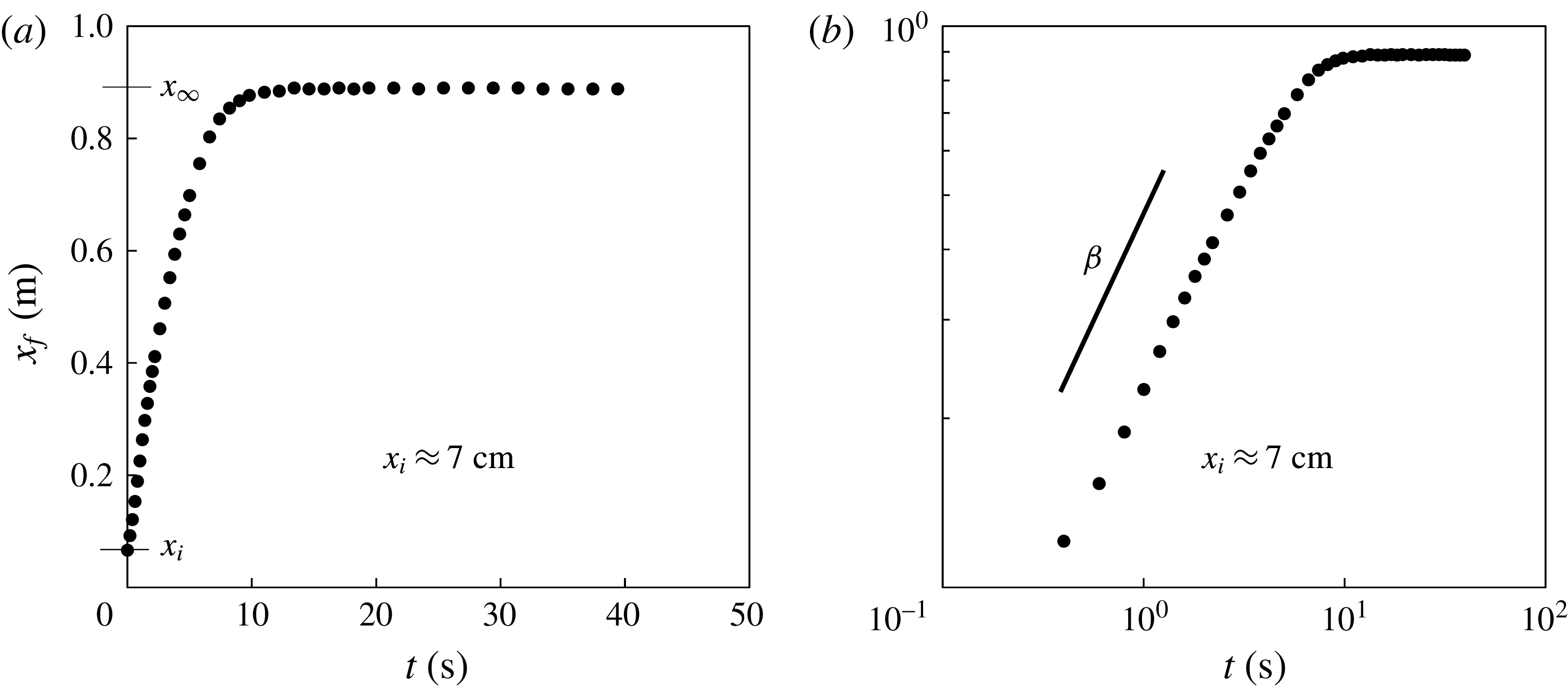
Time evolution of the propagating front in a representative experiment (experiment 1a in table 3). (a) The flow is arrested at long times and a runout distance
 $x_{\infty }$
can be defined. (b) A constant slope
 $\unicode[STIX]{x1D6FD}$
is observed during an intermediate period in the log–log plot, which suggests the scaling of
 $x_{f}(t)\propto t^{\unicode[STIX]{x1D6FD}}$
, with
 $\unicode[STIX]{x1D6FD}\approx 0.6$
in this example.

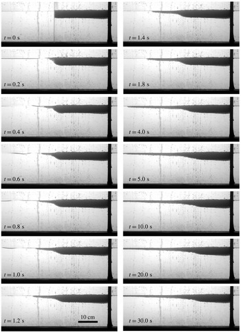
As can be seen from figure 2, the current of beads (soaked in water) propagates along the free surface and culminates in a very shallow front which is one or two beads in thickness. Eventually, in finite time, the front of the beads reaches a maximum location, all motion stops and the interface shape stays unchanged at later times. From the top view, shown in figure 3, we observe that the propagating front of the light beads remains almost planar across the width of the tank. The top view pictures also indicate that the front can become irregular towards the end of the experiments when the spreading rate is very slow, and the effects of surface tension, ambient viscosity and side wall friction may have become significant. Nevertheless, in general, the roughness of the front is small compared with the length of the current, so we neglect the variations of the front across the channel width, and define the front location
 $x_{f}(t)$
based on the side view pictures, shown in figure 2.
In addition, from the top view (figure 3), we observe that the propagating front of the light beads remains almost planar across the width of the tank. The front can become irregular near the end of the experiments, and the effects of surface tension may have become significant. Nevertheless, we neglect the variations of the propagating front across the channel width, and define the front location
 $x_{f}(t)$
based on the side view pictures (figure 2) and provide a detailed quantitative description for the time evolution of the front location
 $x_{f}(t)$
in § 3.2.
When the lock length is small (
 $x_{i}\leqslant 10$
cm) and hence, the initial depth of beads is large, near the origin the interface shape contains a region with an almost constant slope (figure 4). This is different from the observations in the fixed-volume lock-release experiments of Newtonian liquids spreading along a free surface in which the slope remains zero at the origin (Lister & Kerr Reference Lister and Kerr1989). We also note, for small lock lengths, that a shear-driven instability typically appears along the bottom of the current at the beginning of the experiments (figure 4).
When the lock length is large (
 $x_{i}\geqslant 20$
cm) and the initial depth is small, the interface shape contains a ‘frozen region’ near the origin, with an interface shape that remains almost unchanged from its initial state during the entire flow (figure 5). Similar phenomena have also been observed in the fixed-volume lock-release experiments of dry granular materials along a horizontal substrate and the deposits look like a ‘Mexican hat’ (Lajeunesse, Mangeney-Castelnau & Vilotte Reference Lajeunesse, Mangeney-Castelnau and Vilotte2004; Lube et al.
Reference Lube, Huppert, Sparks and Hallworth2004). We also note that a shear-driven instability typically appears at the interface of the water and beads at the beginning of the experiments (figure 4), when the initial lock length is small.
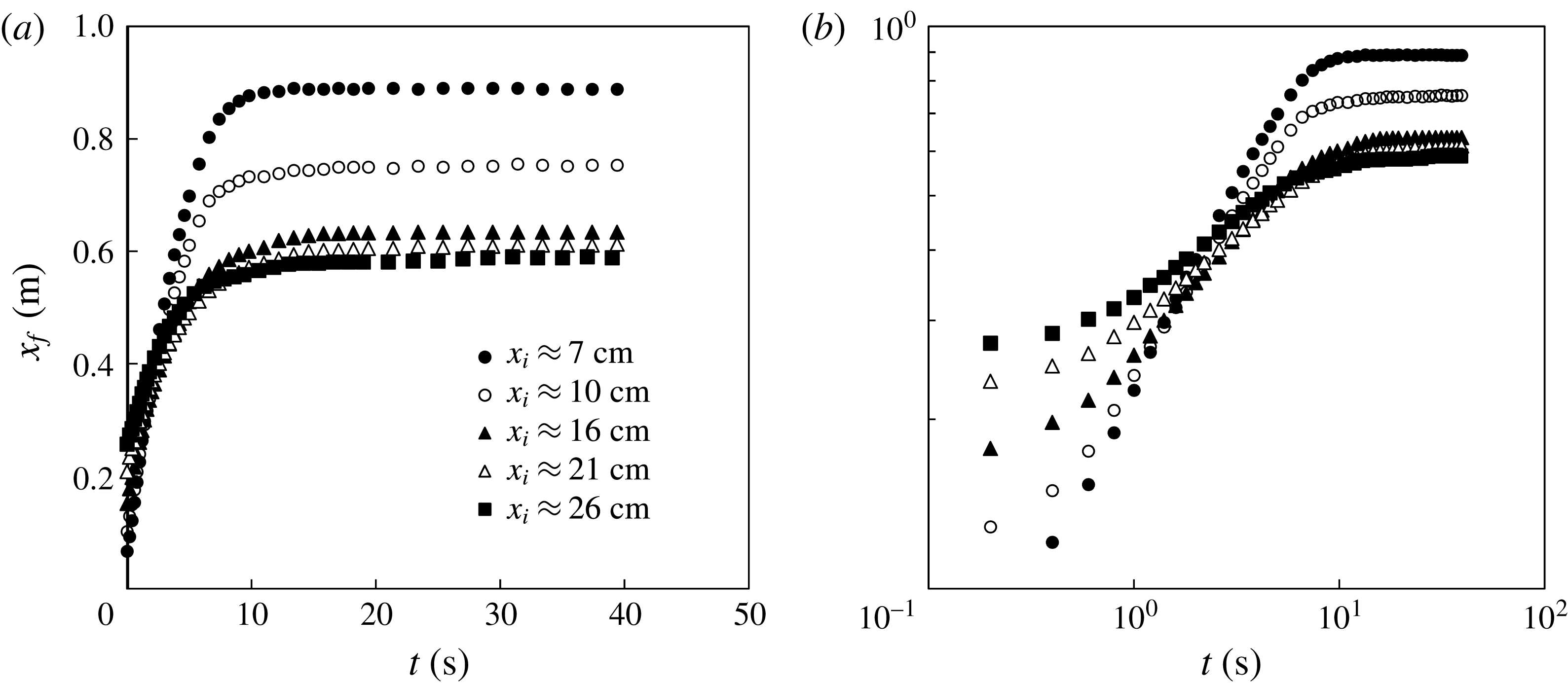
Time evolution of the propagating front
 $x_{f}(t)$
in different experiments, which demonstrates the influence of the lock length. In these experiments, the tank was filled with saturated salt water of depth
 $d=15\pm 0.1$
cm,
 $m=765\pm 1$
g and
 $x_{i}\approx \{7,10,16,21,26\}$
cm. The influence of the lock length
 $x_{i}$
on the runout distance
 $x_{\infty }$
in the arrested state, and scaling exponent
 $\unicode[STIX]{x1D6FD}$
in the intermediate period can be observed.

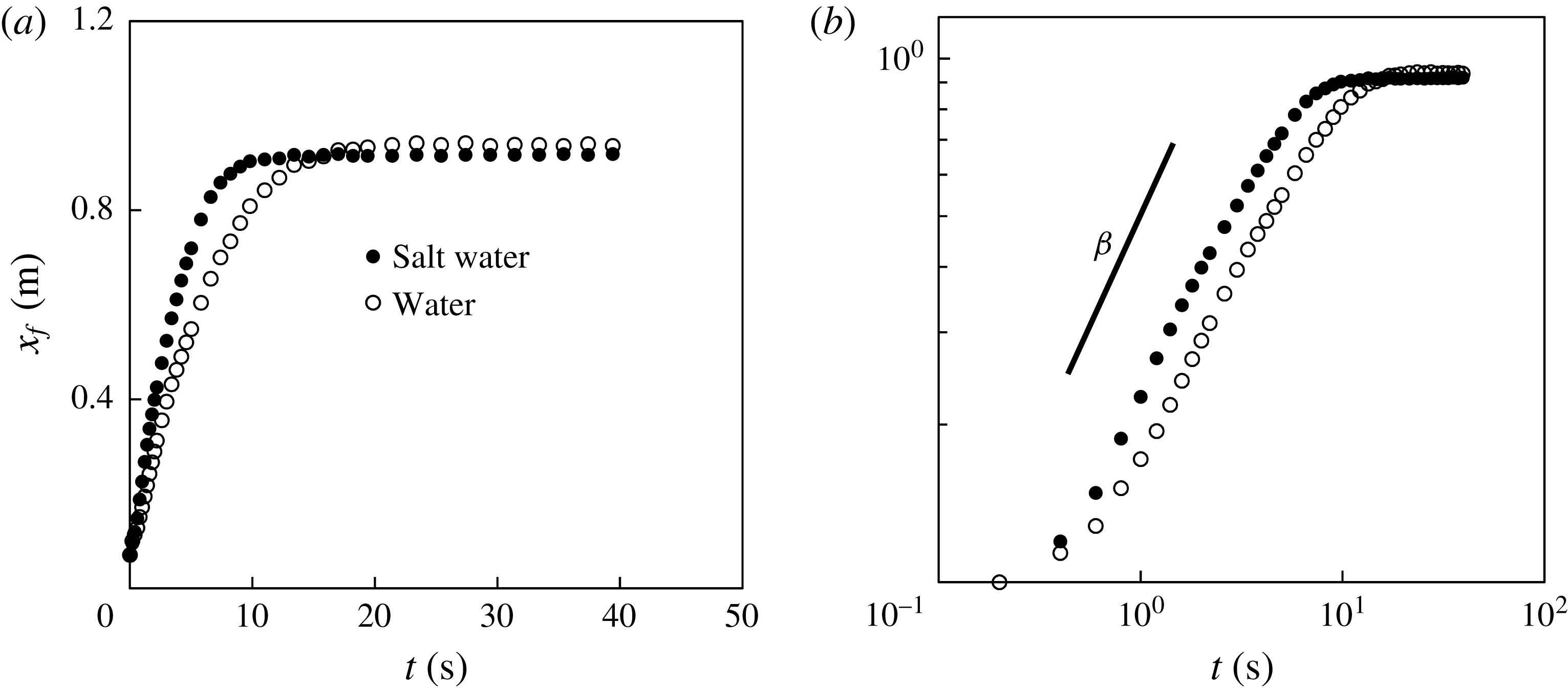
Time evolution of the propagating front
 $x_{f}(t)$
in different experiments, indicating the influence of the density of the ambient liquid. The tank was filled with either water or salt water of depth
 $d=15\pm 0.1$
cm,
 $m=765\pm 1$
g and
 $x_{i}=5$
cm in both experiments. During the intermediate period, when
 $x_{f}(t)=\unicode[STIX]{x1D6FC}t^{\unicode[STIX]{x1D6FD}}$
, the scaling exponent
 $\unicode[STIX]{x1D6FD}$
in both experiments was found to be almost the same, while the prefactor
 $\unicode[STIX]{x1D6FC}$
differed. The runout distances
 $x_{\infty }$
in the two experiments were also slightly different.

3.2 Propagating front
The time evolution of the location of the propagating front
 $x_{f}(t)$
for a representative experiment is shown in figure 6. After an initial acceleration from rest, we observed a constant slope
 $\unicode[STIX]{x1D6FD}$
in the log–log plot during an intermediate time period (
 $1~\text{s}\leqslant t\leqslant 5~\text{s}$
), as shown in figure 6(b), which indicates a scaling behaviour for the front location
 $x_{f}(t)\propto t^{\unicode[STIX]{x1D6FD}}$
. Then the spreading slowed down and the front location approached a final value
 $x_{\infty }$
, defined as the runout distance, as shown in figure 6(a), which corresponds to the final arrested state.
The scaling exponent
 $\unicode[STIX]{x1D6FD}$
in
 $x_{f}(t)=\unicode[STIX]{x1D6FC}t^{\unicode[STIX]{x1D6FD}}$
from different experiments during an intermediate period after the removal of the lock gate: (a) raw data and (b) rescaled data. The rescaled data collapse to a universal curve and the dashed curve represents a best power-law fit. The definition of the scaling exponent
 $\unicode[STIX]{x1D6FD}$
is demonstrated in figure 6(b). The dimensionless lock length is
 $X_{i}\equiv x_{i}/l_{c}$
with the characteristic length scale
 $l_{c}$
defined in (3.1), which accounts for the total mass of the beads
 $m$
.

The influence of the lock length
 $x_{i}$
on the front location
 $x_{f}(t)$
is shown in figure 7. The data show that for a fixed amount of beads, an increase in the initial local length
 $x_{i}$
corresponds to a decrease in both the scaling exponent
 $\unicode[STIX]{x1D6FD}$
during the intermediate period and the runout distance
 $x_{\infty }$
at the final arrested state. We note that the decrease in the runout distance
 $x_{\infty }$
appears progressively weaker, and
 $x_{\infty }$
eventually approaches a constant, as we further increase the lock length
 $x_{i}$
beyond a critical value. We also note that the capillary and other dissipation effects appear to become increasingly significant when we continue to increase the lock length
 $x_{i}$
, as suggested by an irregular propagating front (which contains only one layer of beads) from the top view.
The influence of the fluid density on the front location
 $x_{f}(t)$
is shown in figure 8. During the intermediate period, when the front location obeys
 $x_{f}(t)=\unicode[STIX]{x1D6FC}t^{\unicode[STIX]{x1D6FD}}$
, the scaling exponent
 $\unicode[STIX]{x1D6FD}$
in both experiments appears to be the same, while the prefactor
 $\unicode[STIX]{x1D6FC}$
differs, and a stronger buoyancy effect corresponds to a greater prefactor
 $\unicode[STIX]{x1D6FC}$
. In addition, the runout distances
 $x_{\infty }$
in the two experiments are slightly different, which is not statistically significant.
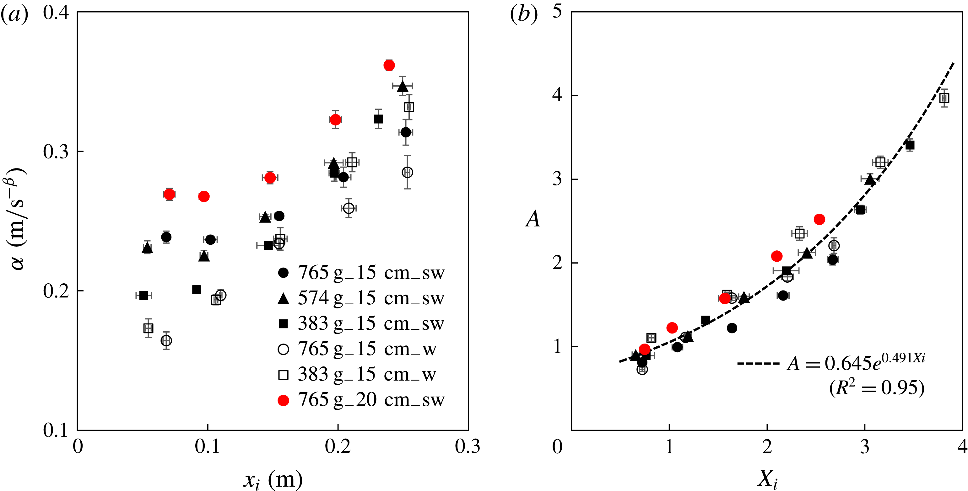
The prefactor
 $\unicode[STIX]{x1D6FC}$
in
 $x_{f}(t)=\unicode[STIX]{x1D6FC}t^{\unicode[STIX]{x1D6FD}}$
from different experiments during the intermediate period after the removal of the lock gate: (a) raw data and (b) rescaled data. The dashed curve is a best exponential fit. The dimensionless lock length is
 $X_{i}\equiv x_{i}/l_{c}$
with the characteristic length scale
 $l_{c}$
defined in (3.1), which accounts for the total mass of the beads
 $m$
. The dimensionless prefactor
 $A\equiv \unicode[STIX]{x1D6FC}/\unicode[STIX]{x1D6FC}_{c}$
with the characteristic scale
 $\unicode[STIX]{x1D6FC}_{c}$
defined in (3.3), includes the effects of both the total mass of beads
 $m$
and the buoyancy
 $\unicode[STIX]{x0394}\unicode[STIX]{x1D70C}g$
.

3.2.1 Scaling exponent
 $\unicode[STIX]{x1D6FD}$

The scaling exponent
 $\unicode[STIX]{x1D6FD}$
is plotted against the lock length in figure 9(a). Within the parameter range we considered, the experiments show a negligible influence of water depth
 $d$
, and buoyancy
 $\unicode[STIX]{x0394}\unicode[STIX]{x1D70C}g$
, where
 $\unicode[STIX]{x0394}\unicode[STIX]{x1D70C}\equiv \unicode[STIX]{x1D70C}_{l}-\unicode[STIX]{x1D70C}_{b}$
is the density difference between liquid and beads. On the other hand, for a fixed mass of beads
 $m$
, the scaling exponent
 $\unicode[STIX]{x1D6FD}$
decreases as the lock length
 $x_{i}$
increases, as mentioned previously. In addition, the total mass of beads
 $m$
has a systematic influence on the scaling exponent
 $\unicode[STIX]{x1D6FD}$
: an increase in
 $m$
corresponds to an increase in
 $\unicode[STIX]{x1D6FD}$
, and the same dependence holds for experiments in both water and salt water.
In order to address the effect of initial mass, we define a dimensionless lock length as
 $X_{i}\equiv x_{i}/l_{c}$
, based on a characteristic length scale
 $l_{c}$
defined by
 $$\begin{eqnarray}\displaystyle l_{c}\equiv \left[\frac{m}{\unicode[STIX]{x1D70C}_{b}w_{t}(1-\unicode[STIX]{x1D719})}\right]^{1/2}=(x_{i}h_{i})^{1/2}, & & \displaystyle\end{eqnarray}$$
where
 $\unicode[STIX]{x1D70C}_{b}$
is the density of the beads,
 $h_{i}$
is the initial vertical extent of the beads in the lock and
 $\unicode[STIX]{x1D719}$
is the porosity of the packed beads (the volume fraction occupied by liquid). We assume that initially the beads are closely packed spheres of equal size and take
 $\unicode[STIX]{x1D719}=0.37$
(Acton, Huppert & Worster Reference Acton, Huppert and Worster2001).
From the definitions of
 $l_{c}$
and
 $X_{i}$
, we obtain that
 $X_{i}=(x_{i}/h_{i})^{1/2}$
, which measures the inverse aspect ratio (height/length) of the initial arrangement of beads. The power-law exponent
 $\unicode[STIX]{x1D6FD}$
is plotted versus
 $X_{i}$
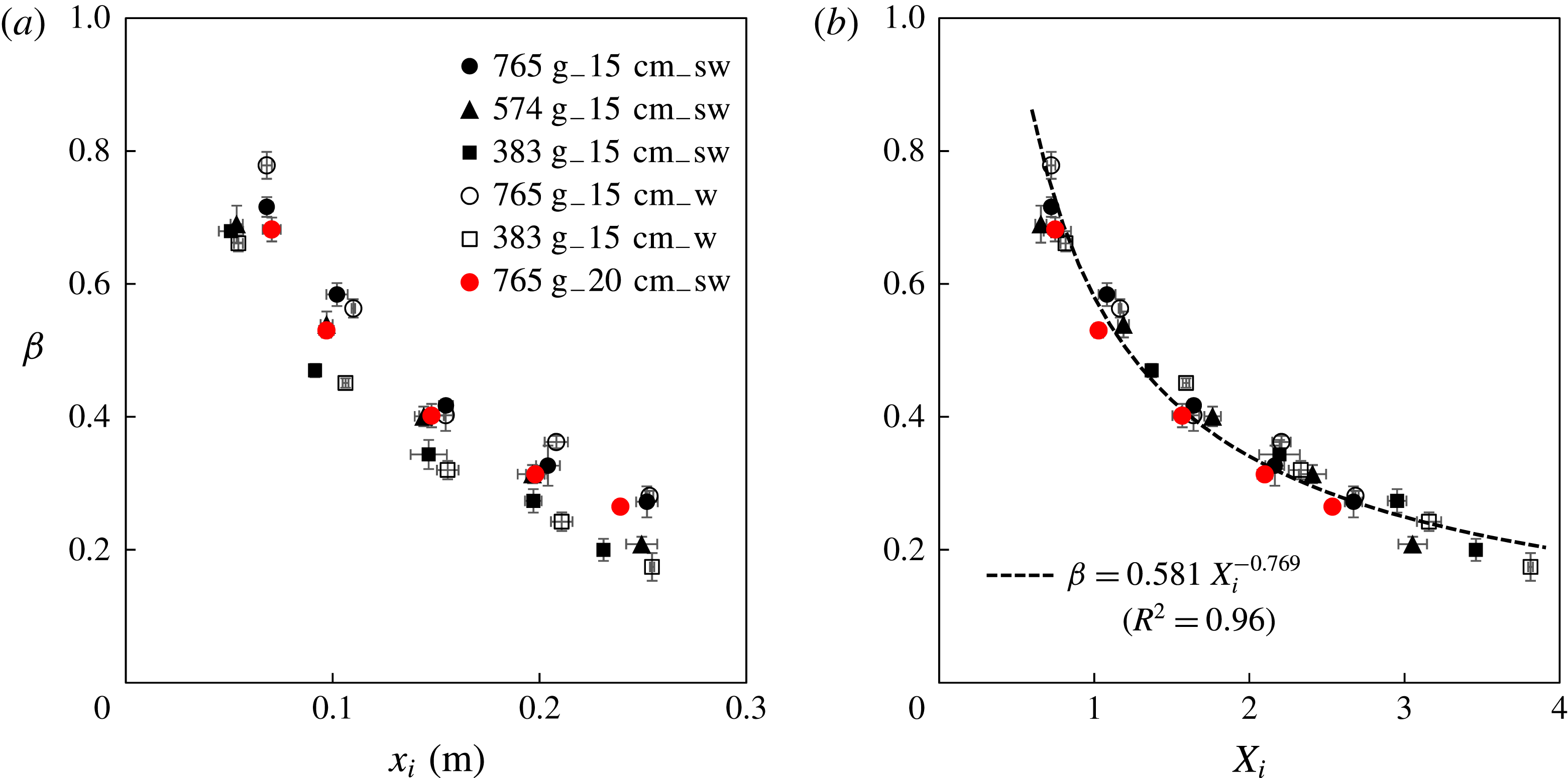
in figure 9(b). This produces a collapse of the data and shows that
 $\unicode[STIX]{x1D6FD}$
decreases as the lock aspect ratio decreases. A least squares best fit of
 $\unicode[STIX]{x1D6FD}$
as a power of
 $X_{i}$
gives
 $$\begin{eqnarray}\displaystyle \unicode[STIX]{x1D6FD}=0.581\,X_{i}^{-0.769},\quad \text{for}~0.6\leqslant X_{i}\leqslant 3.8, & & \displaystyle\end{eqnarray}$$
with
 $R^{2}=0.96$
, and is shown as the dashed curve in figure 9(b). Other fits to the experimental data are provided in appendix B.
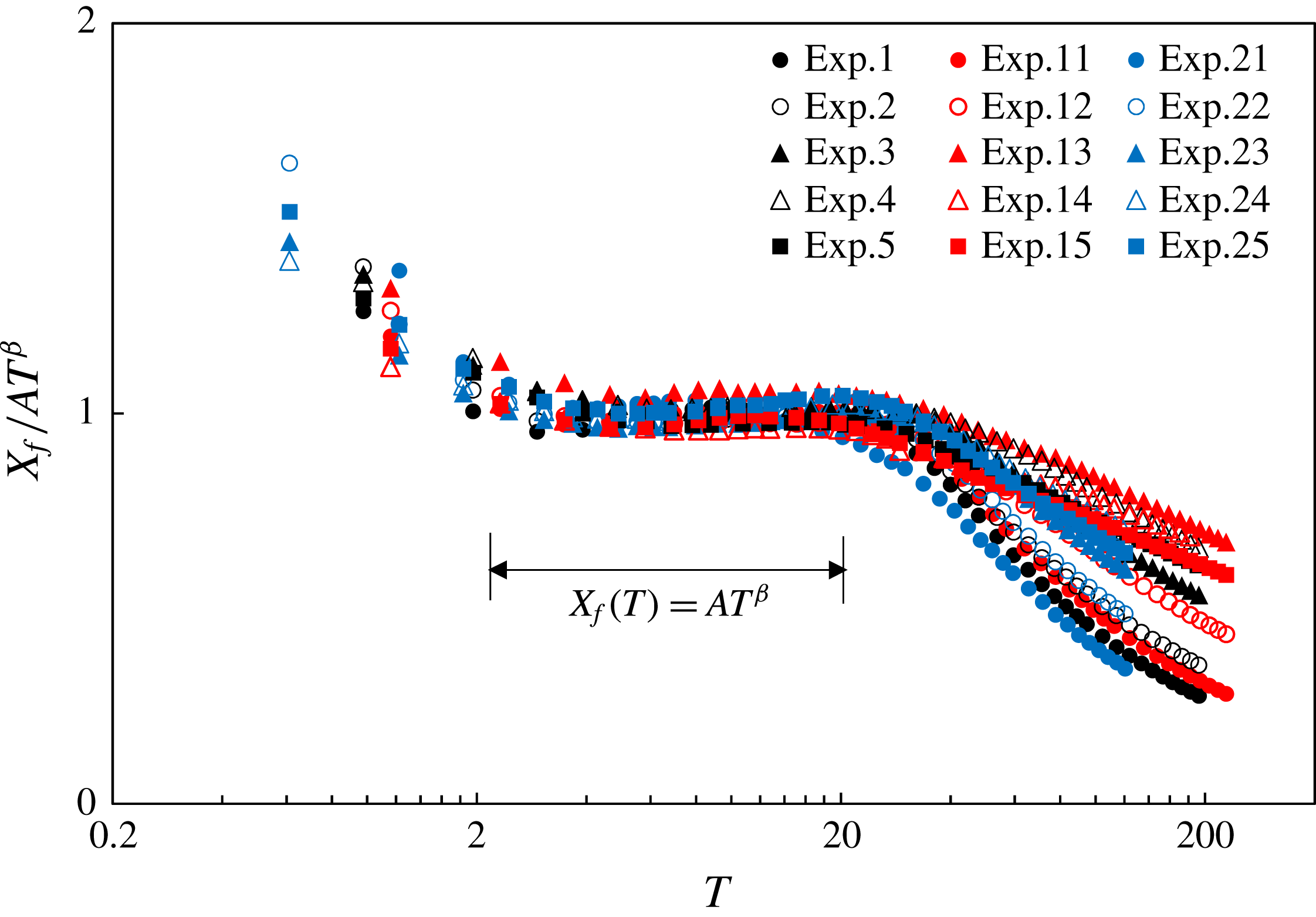
Measurements of the front location rescaled according to
 $X_{f}(T)=AT^{\unicode[STIX]{x1D6FD}}$
. We observe good data collapse in an intermediate time period (approximately
 $2\leqslant T\leqslant 20$
). The approach toward and departure from the scaling behaviour are also demonstrated. The black (
 $m=765\pm 1$
g) and red (
 $m=383\pm 1$
g) symbols indicate experiments in salt water and the blue (
 $m=765\pm 1$
g) symbols represent experiments in fresh water. The experimental parameters are listed in table 3.

3.2.2 Prefactor
$\unicode[STIX]{x1D6FC}$

The prefactor
 $\unicode[STIX]{x1D6FC}$
is plotted against
 $x_{i}$
in figure 10(a). The value of
 $\unicode[STIX]{x1D6FC}$
increases with each of
 $x_{i},m$
and
 $\unicode[STIX]{x0394}\unicode[STIX]{x1D70C}g$
. Clearly, there is a systematic dependence on the initial lock length
 $x_{i}$
, the total mass of beads
 $m$
and the buoyancy
 $\unicode[STIX]{x0394}\unicode[STIX]{x1D70C}g$
. To address these effects, we rescale the lock length
 $x_{i}$
based on the length scale
 $l_{c}$
, defined in (3.1). To find an appropriate characteristic scale for
 $\unicode[STIX]{x1D6FC}$
, we assume that it depends only on the length scale
 $l_{c}$
and the reduced gravity
 $g^{\prime }\equiv \unicode[STIX]{x0394}\unicode[STIX]{x1D70C}g/\unicode[STIX]{x1D70C}_{l}$
, where
 $\unicode[STIX]{x1D70C}_{l}$
is the density of the liquid in the tank and
 $\unicode[STIX]{x1D70C}_{l}=\unicode[STIX]{x1D70C}_{w}$
or
 $\unicode[STIX]{x1D70C}_{sw}$
, respectively. Dimensional analysis suggests that we can define a dimensionless prefactor
 $A\equiv \unicode[STIX]{x1D6FC}/\unicode[STIX]{x1D6FC}_{c}$
, where
 $$\begin{eqnarray}\displaystyle \unicode[STIX]{x1D6FC}_{c}\equiv g^{\prime (\unicode[STIX]{x1D6FD}/2)}l_{c}^{1-(\unicode[STIX]{x1D6FD}/2)}=\left(\frac{\unicode[STIX]{x0394}\unicode[STIX]{x1D70C}g}{\unicode[STIX]{x1D70C}_{l}}\right)^{\unicode[STIX]{x1D6FD}/2}\left[\frac{m}{\unicode[STIX]{x1D70C}_{b}w_{t}(1-\unicode[STIX]{x1D719})}\right]^{1/2-\unicode[STIX]{x1D6FD}/4}. & & \displaystyle\end{eqnarray}$$
We plot the rescaled prefactor
 $A$
as a function of the rescaled lock length
 $X_{i}$
in figure 10(b). This scaling collapses the data and shows that
 $\unicode[STIX]{x1D6FC}$
decreases as the aspect ratio of the initial bead configuration increases (figure 10
b). A best exponential fit for the data is
 $$\begin{eqnarray}\displaystyle A=0.645\,e^{0.491X_{i}},\quad \text{for}~0.6\leqslant X_{i}\leqslant 3.8, & & \displaystyle\end{eqnarray}$$
with
 $R^{2}=0.95$
, and is shown as the dashed curve in figure 10(b). Other best fits using different functional forms of
 $A$
versus
 $X_{i}$
are given in appendix B.
3.2.3 Propagation law
The length scale
 $l_{c}$
and reduced gravity
 $g^{\prime }$
provide a characteristic time scale
 $$\begin{eqnarray}\displaystyle t_{c}\equiv \left(\frac{l_{c}}{g^{\prime }}\right)^{1/2}=\left(\frac{\unicode[STIX]{x0394}\unicode[STIX]{x1D70C}g}{\unicode[STIX]{x1D70C}_{l}}\right)^{-1/2}\left[\frac{m}{\unicode[STIX]{x1D70C}w_{t}(1-\unicode[STIX]{x1D719})}\right]^{1/2}. & & \displaystyle\end{eqnarray}$$
Defining a dimensionless time
 $T\equiv t/t_{c}$
and a dimensionless front location
 $X_{f}(T)\equiv x_{f}/l_{c}$
, the time evolution of the front location
 $x_{f}(t)=\unicode[STIX]{x1D6FC}t^{\unicode[STIX]{x1D6FD}}$
can be rewritten in dimensionless form
 $$\begin{eqnarray}\displaystyle X_{f}(T)=AT^{\unicode[STIX]{x1D6FD}}. & & \displaystyle\end{eqnarray}$$
The front locations rescaled according to (3.6) are shown in figure 11. As expected the data collapse during the period of power-law spreading (
 $2\leqslant T\leqslant 20$
). The approach toward and departure from the scaling behaviour are also demonstrated in figure 11. We also note that the collapse of data measuring the distance of the front from the lock gate does not collapse as well.
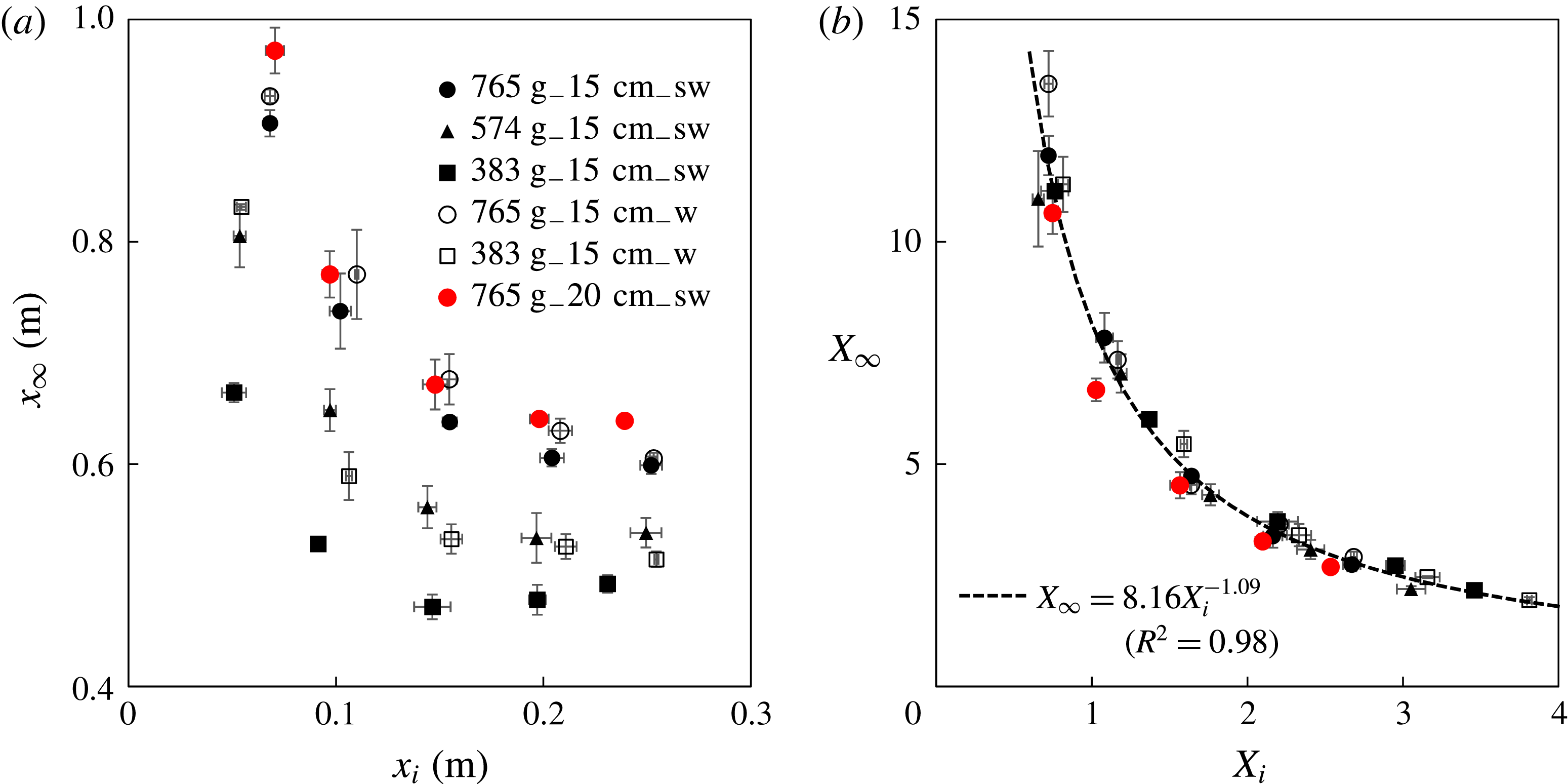
The final runout distance
 $x_{\infty }$
: (a) raw data and (b) rescaled data. The definition of the runout distance
 $x_{\infty }$
is shown in figure 6(a). The dashed curve is a best power-law fit. The dimensionless runout distance and lock length are is defined as
 $X_{\infty }\equiv x_{\infty }/l_{\infty }$
and
 $X_{i}\equiv x_{i}/l_{c}$
, respectively, with
 $l_{\infty }$
and
 $l_{c}$
defined in (3.7) and (3.1).

3.3 Runout distance
$x_{\infty }$

The final runout distance
 $x_{\infty }$
is shown in figure 12(a). For short lock lengths
 $x_{\infty }$
decreases with increasing
 $x_{i}$
, but is almost independent of lock length for
 $x_{i}>15$
cm. There is only a small difference between the fresh and salt water data, but
 $x_{\infty }$
increases with
 $m$
. Since the extension of the current occurs during the inertial spreading phase, a runout length scale
 $l_{\infty }$
can be defined as
 $$\begin{eqnarray}\displaystyle l_{\infty }\equiv \unicode[STIX]{x1D6FC}t_{c}^{\unicode[STIX]{x1D6FD}}=Al_{c}=A\left[\frac{m}{\unicode[STIX]{x1D70C}_{b}w_{t}(1-\unicode[STIX]{x1D719})}\right]^{1/2}. & & \displaystyle\end{eqnarray}$$
We define a dimensionless runout distance
 $X_{\infty }\equiv x_{\infty }/l_{\infty }$
, and plot
 $X_{\infty }$
as a function of the dimensionless lock length
 $X_{i}$
in figure 12(b). This scaling collapses the data and shows that
 $X_{\infty }$
increases with the initial aspect ratio of the bead configuration, and is independent of the buoyancy of the beads. The best power-law fit, shown as the dashed curve in figure 12(b), is given by
 $$\begin{eqnarray}\displaystyle X_{\infty }=8.16\,X_{i}^{-1.09},\quad \text{for}~0.6\leqslant X_{i}\leqslant 3.8, & & \displaystyle\end{eqnarray}$$
with
 $R^{2}=0.98$
. Other data-fitting results, using different functional forms of
 $X_{\infty }$
versus
 $X_{i}$
, are also provided in appendix B.
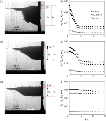
(a,c,e) Profile shapes at
 $t=0.6$
s for three representative experiments, and the definition of the maximum thicknesses
 $h_{0t}$
,
 $h_{0b}$
and
 $h_{0}$
. (b,d,f) Time evolution of the corresponding
 $h_{0t}$
,
 $h_{0b}$
. The tank was filled with saturated salt water of depth
 $d=15\pm 0.1$
cm,
 $m=765\pm 1$
g and (a,b)
 $x_{i}=10$
cm, (c,d)
 $x_{i}=15$
cm, and (e,f)
 $x_{i}=20$
cm.

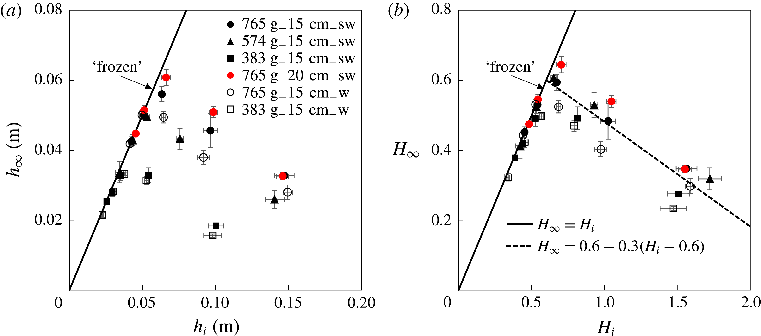
The maximum thickness
 $h_{\infty }\equiv h_{0}(t\rightarrow \infty )$
versus the initial height
 $h_{i}\equiv h_{0}(t=0)$
of the spreading beads at the origin
 $x=0$
: (a) raw data and (b) rescaled data. In (b) the dimensionless thicknesses are defined as
 $H_{\infty }\equiv h_{\infty }/l_{c}$
and
 $H_{i}\equiv h_{i}/l_{c}$
, respectively. The solid line in the figure indicates that the maximum thickness
 $h_{0}$
remains unchanged during the experiments with
 $0.3\leqslant H_{i}\leqslant 0.6$
, which corresponds to the existence of a ‘frozen’ region near the origin as shown in figure 5. The dashed line in (b) is given by (3.9).

Although viscous and surface tension effects may be expected to become important when the spreading rate is slow as the current approaches its final arrested position, the collapse of the data shown in figure 12(b) suggests that the runout distance
 $x_{\infty }$
is determined during the inertial-dominated period. We also note that the two dimensional effects, i.e. the irregularity of the propagating front across the channel width are larger with increasing lock length
 $x_{i}$
, decreasing
 $m$
and decreasing buoyancy
 $\unicode[STIX]{x0394}\unicode[STIX]{x1D70C}g$
.
3.4 Maximum thicknesses
The time evolution of the maximum thicknesses, defined at the back wall of the lock as the distances between the water level and the top surface
 $h_{0t}$
and the bottom surface
 $h_{0b}$
of the beads, respectively, are shown in figure 13. For small lock lengths
 $x_{i}<15$
cm (e.g. experiment 1a and experiment 2a) both
 $h_{0t}$
and
 $h_{bt}$
initially decreased and then became constant as the current approached its final arrested state. For longer lock length
 $x_{i}\geqslant 20$
cm (e.g., experiment 3a) both
 $h_{0t}$
and
 $h_{0b}$
remained close to their initial values, which corresponds to the existence of the ‘frozen’ region near the origin, as shown in figure 5.
The final thickness
 $h_{\infty }\equiv h_{0}(t\rightarrow \infty )$
at the rear wall of the lock is plotted in figure 14(a) as a function of initial height
 $h_{i}\equiv h_{0}(t=0)$
(figure 13). The solid line in the figure indicates the limit that
 $h_{0}$
remains unchanged during an experiment, which corresponds to the existence of a near origin ‘frozen’ regime, as shown in figure 5.
The final thickness shows a systematic increase with the mass of beads
 $m$
(figure 14
a). In order to account for this we define dimensionless final thickness as
 $H_{\infty }\equiv h_{\infty }/l_{c}$
and initial height as
 $H_{i}\equiv h_{i}/l_{c}=1/X_{i}$
, and plot the dimensionless
 $H_{\infty }$
versus
 $H_{i}$
in figure 14(b). This reduces the variation associated with different
 $m$
, and a universal curve of
 $H_{\infty }$
versus
 $H_{i}$
is obtained, which can be approximated by
 $$\begin{eqnarray}\displaystyle H_{\infty }=\left\{\begin{array}{@{}ll@{}}H_{i}, & 0.3\leqslant H_{i}\leqslant 0.6,\\ 0.6-0.3(H_{i}-0.6), & 0.6\leqslant H_{i}\leqslant 1.7.\end{array}\right. & & \displaystyle\end{eqnarray}$$
This relationship is plotted in figure 14(b). The solid line indicates that the maximum thickness
 $H_{0}$
remains unchanged when
 $0.3\leqslant H_{i}\leqslant 0.6$
(
 $1.7\leqslant X_{i}\leqslant 3.8$
), while the dashed line provides a reasonable approximation for
 $H_{\infty }$
for
 $0.6\leqslant H_{i}\leqslant 1.7$
(
 $0.6\leqslant X_{i}\leqslant 1.7$
). There appears to be a weaker but systematic buoyancy effect, i.e. an increase in
 $H_{\infty }$
with
 $\unicode[STIX]{x0394}\unicode[STIX]{x1D70C}g$
, which is not captured by the current scaling.
Summary of the major findings for the time-dependent non-dimensional front location
 $X_{f}$
, the runout distance
 $X_{\infty }$
and the final thickness at the origin
 $H_{\infty }$
. We note that some of the fitted powers are close to rational fractions.

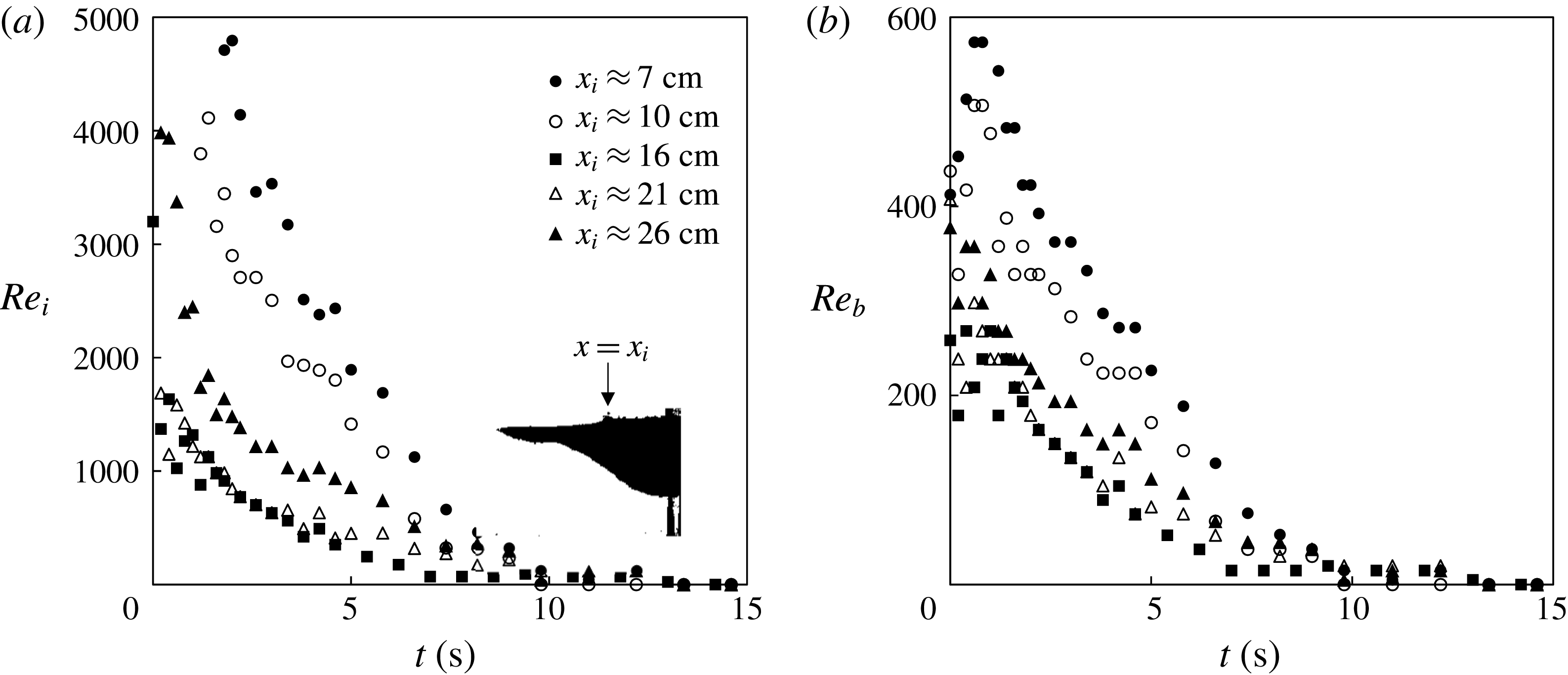
More details of the experiments are provided in appendix A. The Reynolds numbers
 $Re$
based on the current thickness or an individual bead were
 $Re\gg 1$
during the intermediate time period (e.g.
 $1~\text{s}\leqslant t\leqslant 5~\text{s}$
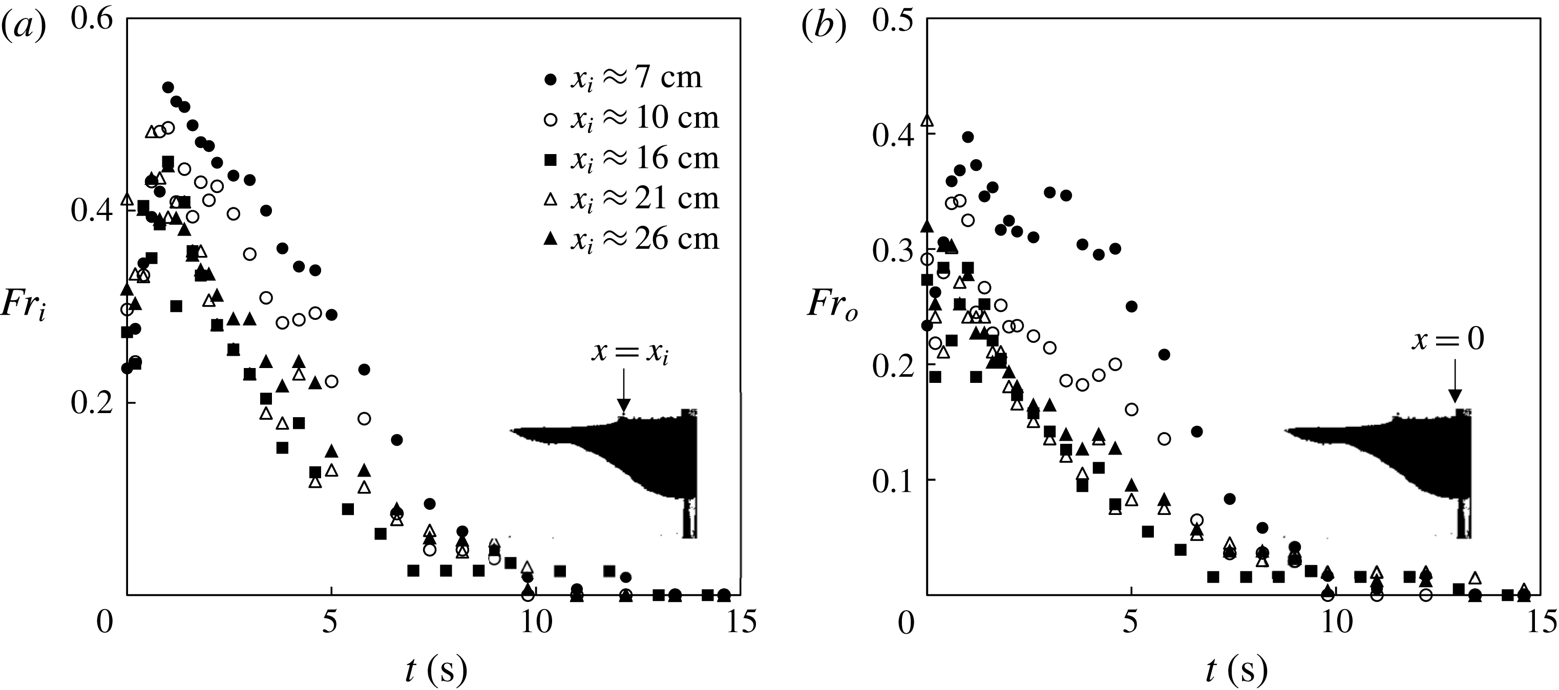
), when the front propagates according to a power-law behaviour, indicating that the current is inertial during this phase. Also, motivated by the front constraining condition of a high Reynolds number gravity current, we computed the Froude number
 $Fr$
for the experiments, e.g. based on the bead layer thickness at the origin, and we found that, after a short initial transition (e.g. 1 s),
 $Fr$
decreases as time progresses, and
 $Fr<0.5$
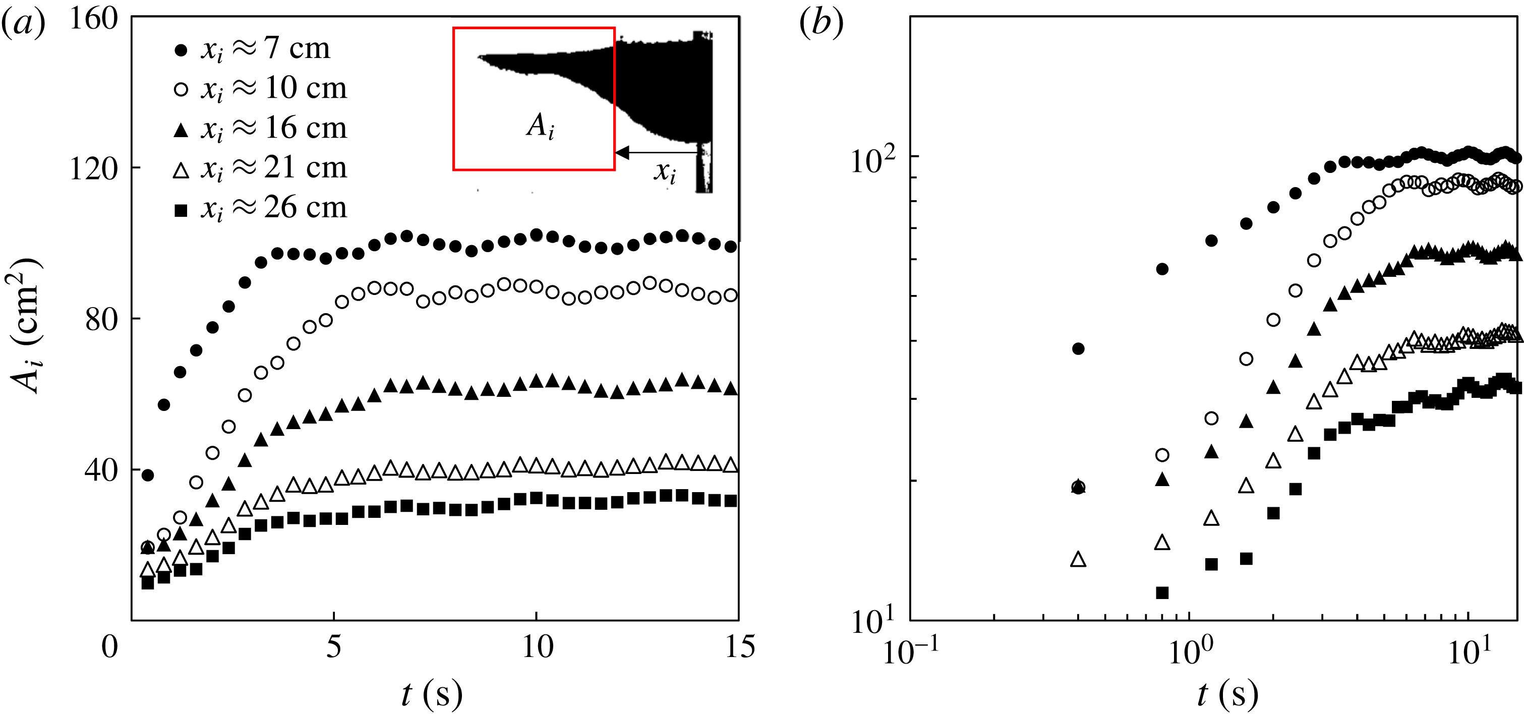
during the majority of the time evolution. This suggests that the condition for an inertial current, that the frontal Froude number is constant and of order one (see, e.g. Simpson Reference Simpson1982) is not appropriate in this situation. In addition, based on the side view pictures, we calculated the time evolution of the intruding area
 $A_{i}$
, measured between the location of the lock gate and the propagating front
 $x_{f}(t)$
. We observe that
 $A_{i}$
first increases, following the removal of the lock gate, and gradually reaches a constant at long times (e.g.
 $t=30$
s). However, to within fairly coarse resolution, we are unable to constrain any variations in the mean porosity of the current, and therefore cannot speculate further as to the evolution of the effective rheology of the current during the course of the experiments.
4 Summary and discussions
4.1 Summary
In this paper, we investigated the dynamics of a current of spreading beads upon release from behind a lock gate into a liquid of greater density. There are few previous studies on such granular flows despite a rich set of related geophysical and environmental phenomena such as debris flows, industrial waste outputs and volcanic ash spreading. We focused on the time evolution of the front location and the interface shape between the current of beads and the ambient liquid and provided a systematic experimental exploration on the effects of lock length, total amount of beads, and the density of the ambient liquids. We presented scaling arguments to address the major physics that controls the time-dependent front location, the finite runout distance and maximum thickness of the bead layer. The rescaled experimental data collapse to universal curves, which can be used to describe the dynamic behaviour of these flows. The major findings are summarized in table 1. We note that some of the fitted powers are close to rational fractions.
While we provide experimental and scaling results for the front dynamics, further theoretical work is necessary to investigate the detailed functional forms of the dependence of the scaling exponent
 $\unicode[STIX]{x1D6FD}$
, the prefactor
 $A$
, the runout distance
 $X_{\infty }$
and the maximum thickness
 $H_{\infty }$
on the initial lock length
 $X_{i}$
, respectively. Theoretical work is also needed to address the time evolution of the profile shape of the current of beads, the packing efficiency and the existence of the irregular front patterns (figure 3), the shear-driven instability (figure 4), and the ‘frozen’ region (figure 5) in different flow situations.
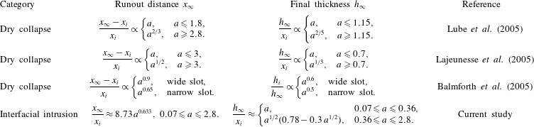
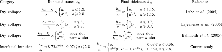
A summary of previous and current experimental measurements on the runout distance
 $x_{\infty }$
and final thickness at the origin
 $h_{\infty }$
in dry granular collapse and granular intrusion problems. Here
 $a\equiv h_{i}/x_{i}$
, which represents the initial aspect ratio. Note we have rewritten the experimental results of the current study in terms of the aspect ratio in the table, and we have used
 $A\approx 1.07\,X_{i}^{0.824}$
(appendix B) instead of
 $A\approx 0.926\,e^{-0.455X_{i}}$
for the runout distance.
4.2 Discussion
The study has shed light on a category of problems that address the flow of granular materials along a free surface of a liquid, and is expected to motivate further research. Before we close the paper, it is worthwhile to note some major differences between this flow and three other related phenomena: dry and immersed granular collapses in liquids of lower density, the intrusive gravity current, and the particle-laden gravity current. We provide a brief summary in this section.
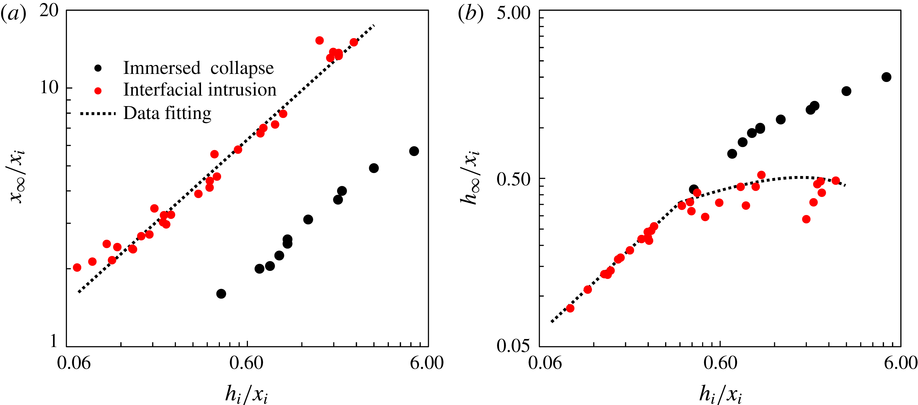
Experimental measurements for the (a) runout distance and (b) final thickness for immersed granular collapse (Rondon et al. Reference Rondon, Pouliquen and Aussillous2011) and interfacial granular intrusion (current study). The expressions for the fitting curves are given in table 2.

The time evolution of
 $Re$
in representative experiments: (a)
 $Re_{i}\equiv uh_{i}/\unicode[STIX]{x1D708}$
with
 $h_{i}$
denoting the thickness of the beads at the location of the lock gate
 $x_{i}$
and (b)
 $Re_{b}\equiv 2ur/\unicode[STIX]{x1D708}$
based on the diameter of the beads. The experiments are identical to those in figure 7.

(i) A granular density current along a free surface differs in a number of aspects from the dry granular collapse or immersed granular collapse in liquids of lower density. For example, there is no basal friction in the flow along the free surface, although surface tension may play a role, particularly as the current comes to rest. The runout distance of the experiments in this study can be estimated as the maximum horizontal extension of the intermediate period (3.7), during which the location of the spreading front follows a power-law time dependence (3.6). However, since the arrested front is only one or two beads thick we expect an increasing role of capillary forces when the granular current slows down. This surface tension may be responsible for the irregular front patterns (figure 3), observed at the end of some of the experiments. In comparison, the granular collapse experiments do not exhibit such behaviours either in dry collapse (Balmforth & Kerswell Reference Balmforth and Kerswell2005; Lajeunesse, Monnier & Homsy Reference Lajeunesse, Monnier and Homsy2005; Lube et al. Reference Lube, Huppert, Sparks and Freundt2005) or immersed collapse in a liquid of lower density (Pailha et al. Reference Pailha, Nicolas and Pouliquen2008; Rondon et al. Reference Rondon, Pouliquen and Aussillous2011). Table 2 summarizes the experimental results on the runout distance and final thickness in previous studies of dry granular collapse, which provides a comparison with the current work. In addition, we show in figure 15 the experimental data from immersed granular collapse (from figure 11 in Rondon et al. Reference Rondon, Pouliquen and Aussillous2011) and the current study. The comparison indicates that without basal friction the runout distance in the bead current is greater than that in immersed granular collapse.
(ii) For an intrusive gravity current, the front of the invading fluid continues to propagate, going through an inertial (Holyer & Huppert Reference Holyer and Huppert1980; de Rooij et al. Reference de Rooij, Linden and Dalziel1999) and then a viscous regime (Lister & Kerr Reference Lister and Kerr1989). After an initial brief period of acceleration, the front of the intrusion travels at a constant speed for multiple lock lengths before decelerating (Maxworthy et al. Reference Maxworthy, Leilich, Simpson and Meiburg2002; Maurer et al. Reference Maurer, Bolster and Linden2010), during which time the frontal
$Fr$
is constant and of order one. However, for granular flows at a free interface, there is no period of constant speed but, instead, the front decelerates and the location of the propagating front follows a power-law time dependence before coming to rest (figures 6–8). Although
$Re\gg 1$
during the spreading of the beads (figure 16),
$Fr$
decreases monotonically (figure 17), which suggests that the constant
$Fr$
condition is not appropriate during the propagation of a current of beads.(iii) A granular current along a free surface is also significantly different from the standard particle-laden gravity current. In both flow situations, the buoyant currents reach a finite runout distance. However, for granular current along a free surface, the particles are typically close to each other, and the profile shape of a granular current is set by the envelope of the closely located particles (figure 2), and the size of the beads sets the lower limit for the thickness of the bead layer. In comparison, in high Reynolds number particle-laden flows, the particles do not pack and are often assumed to distribute homogeneously within the current because of mixing effects. The buoyancy-driven flow eventually stops because the density of the current (an ‘average’ of the particle–fluid system) continues to decrease due to the fallout of the particles, and the sedimentation speed is determined by a balance between buoyancy and viscous drag (see, e.g. Bonnecaze et al. Reference Bonnecaze, Huppert and Lister1993).


The time evolution of
 $Fr$
in representative experiments: (a)
 $Fr_{i}\equiv u/\sqrt{g^{\prime }h_{i}}$
with
 $h_{i}$
denoting the thickness of the beads at the location of the lock gate
 $x_{i}$
and (b)
 $Fr_{0}\equiv u/\sqrt{g^{\prime }h_{0}}$
with
 $h_{0}$
representing the thickness of the beads at the origin
 $x=0$
.
 $u$
is the propagating speed of the front of the current of beads, and
 $g^{\prime }$
is the reduced gravity. The experiments are identical to those in figure 7.

Acknowledgements
Z.Z. is grateful for the support of a David Crighton Fellowship from the Department of Applied Mathematics and Theoretical Physics (DAMTP) at the University of Cambridge. J.A.N. is supported by a Royal Society University Research Fellowship. N.M.V. is supported by a Royal Society Dorothy Hodgkin Fellowship. We appreciate the helpful discussions with T. Ball, S. Dalziel, N. O’Keeffe, B. Rallabandi, J. M. F. Tsang and A. Thomas. We also thank M. Hallworth, D. Page-Croft, and the technicians in the GK Batchelor Laboratory in DAMTP for their help with the set-up of the experimental apparatus.
Summary of the experimental parameters. All experiments were conducted in a rectangular tank of length
 $l_{t}=2.09\pm 0.01$
m, width
 $w_{t}=0.15\pm 0.01$
m and depth
 $d_{t}=0.57\pm 0.01$
m. Either saturated salt water (saturated NaCl solution), with density
 $\unicode[STIX]{x1D70C}_{sw}=1180~\text{kg}~\text{m}^{-3}$
, or fresh water, with density
 $\unicode[STIX]{x1D70C}_{w}=998~\text{kg}~\text{m}^{-3}$
, was used in the experiments. The depth
 $d$
of the liquid, the total mass of the beads
 $m$
, and the lock length
 $x_{i}$
were also varied, as listed in the table. Spherical polypropylene beads (McMaster Carr, 1974K2) were used in all the experiments with a radius
 $r=1.59$
mm and density
 $\unicode[STIX]{x1D70C}_{b}=910~\text{kg}~\text{m}^{-3}$
, measured at room temperature. Experiments with similar parameters were conducted to test the reproducibility.
Summary of experimental results. The experimental data for the time evolution of the front location are fitted to a power-law form of
 $x_{f}(t)=\unicode[STIX]{x1D6FC}t^{\unicode[STIX]{x1D6FD}}$
during an intermediate time period. The values of the scaling exponent
 $\unicode[STIX]{x1D6FD}$
and the prefactor
 $\unicode[STIX]{x1D6FC}$
from a best least-squares fit of the experimental data are reported. The runout distance
 $x_{\infty }$
represents the length of the beads at the end of the experiments, once the motion has stopped. The initial thickness represents the thickness of the beads at the origin
 $x=0$
at the beginning of the experiments, i.e.
 $h_{i}\equiv h_{0}(t=0)$
, while the final thickness
 $h_{\infty }$
represents the thickness of the beads at
 $x=0$
at the end of the experiments, i.e.
 $h_{\infty }\equiv h_{0}(t\rightarrow \infty )$
, as shown in figure 13.

Appendix A. Additional experimental details
We provide more details on the experiments in this Appendix. We first summarize the experimental parameters and results in tables 3 and 4. We calculate the time evolution of the Reynolds number
 $Re$
and Froude number
 $Fr$
in different flow situations in § A.1. We also provide estimates for the changes of effective porosity
 $\unicode[STIX]{x1D719}_{e}$
and intruding area
 $A_{i}$
between the location of the lock gate and the front of the bead layer in § A.2.
A.1 On Reynolds number
$Re$
and Froude number
$Fr$


The time evolution of the Reynolds number
 $Re$
during the experiments is shown in figure 16. In particular, based on the thickness
 $h_{i}$
of the bead layer at the location of the lock,
 $x_{i}$
, and the diameter of the beads,
 $2r$
, we define Reynolds numbers by
 $$\begin{eqnarray}\displaystyle Re_{i}\equiv \frac{uh_{i}}{\unicode[STIX]{x1D708}},\quad \text{and}\quad Re_{b}\equiv \frac{2ur}{\unicode[STIX]{x1D708}}, & & \displaystyle\end{eqnarray}$$
where
 $u$
is the speed of the propagating front, and
 $\unicode[STIX]{x1D708}$
is the kinematic viscosity of the liquid. We note that when the front location follows a power-law behaviour (e.g.
 $1~\text{s}\leqslant t\leqslant 5~\text{s}$
), the
 $Re\gg 1$
, which suggests that the flow can be considered inviscid during this intermediate period.
We also calculate the time evolution of the Froude number
 $Fr$
in representative experiments. The definition of
 $Fr$
depends on where we measure the thickness of the current of beads. In particular, since it is difficult to identify a head region and a corresponding thickness near the front of the current of beads, we provide two calculations based on the thickness of beads
 $h_{i}(t)$
at the location of the lock gate
 $x=x_{i}$
and the thickness
 $h_{0}(t)$
at the origin
 $x=0$
, as shown in figure 17. The definitions of
 $Fr$
are
 $$\begin{eqnarray}\displaystyle Fr_{i}\equiv \frac{u}{\sqrt{g^{\prime }h_{i}}},\quad \text{and}\quad Fr_{0}\equiv \frac{u}{\sqrt{g^{\prime }h_{0}}}, & & \displaystyle\end{eqnarray}$$
where
 $u$
represents the propagating speed of the front of the current of beads and
 $g^{\prime }$
is the reduced gravity. The representative experiments are identical to those shown in figure 7 and were all conducted in salt water with depth
 $d=15\pm 1$
cm. The total mass of beads is
 $m=765\pm 1$
g, while the lock length was varied as
 $x_{i}\approx \{5,10,15,20,25\}$
cm. The calculation indicates that after a short initial transition (e.g. 1 s),
 $Fr$
decreases monotonically as time progresses, and
 $Fr<0.5$
during most of the time period. We note that the frontal
 $Fr$
is constant and of order one for an inertial current (see, e.g. Simpson Reference Simpson1982), and our calculation suggests that this constant frontal Froude number condition is not appropriate for the spreading of the current of beads. Generally, we do not expect the Froude number to be a relevant parameter for these flows.
A.2 On porosity
$\unicode[STIX]{x1D719}_{e}$
and intruding area
$A_{i}$


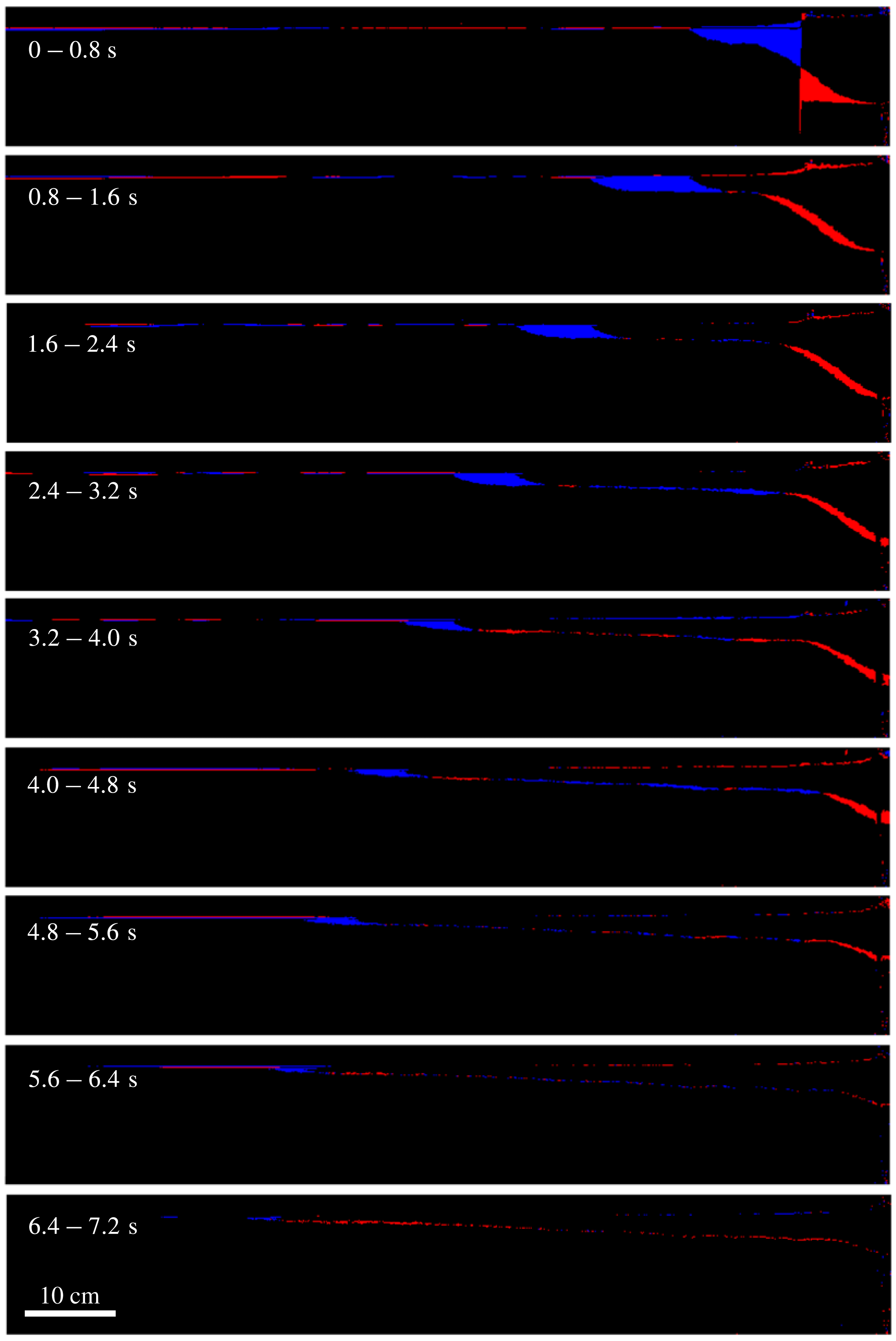
The incremental change of area of the bead layer for the experiment shown in figure 2. The blue region represents an increase in area, while the red region indicates a decrease. The downstream signals represent small changes in the free surface height.

Calculations based on side view pictures in representative experiments (a) area
 $A_{e}$
for the current of beads and (b) porosity
 $\unicode[STIX]{x1D719}_{e}$
, computed by
 $\unicode[STIX]{x1D719}_{e}\equiv 1-m/(\unicode[STIX]{x1D70C}_{b}w_{t}A_{e})$
, where
 $m$
and
 $\unicode[STIX]{x1D70C}_{b}$
are the mass and density of the beads, respectively, and
 $w_{t}$
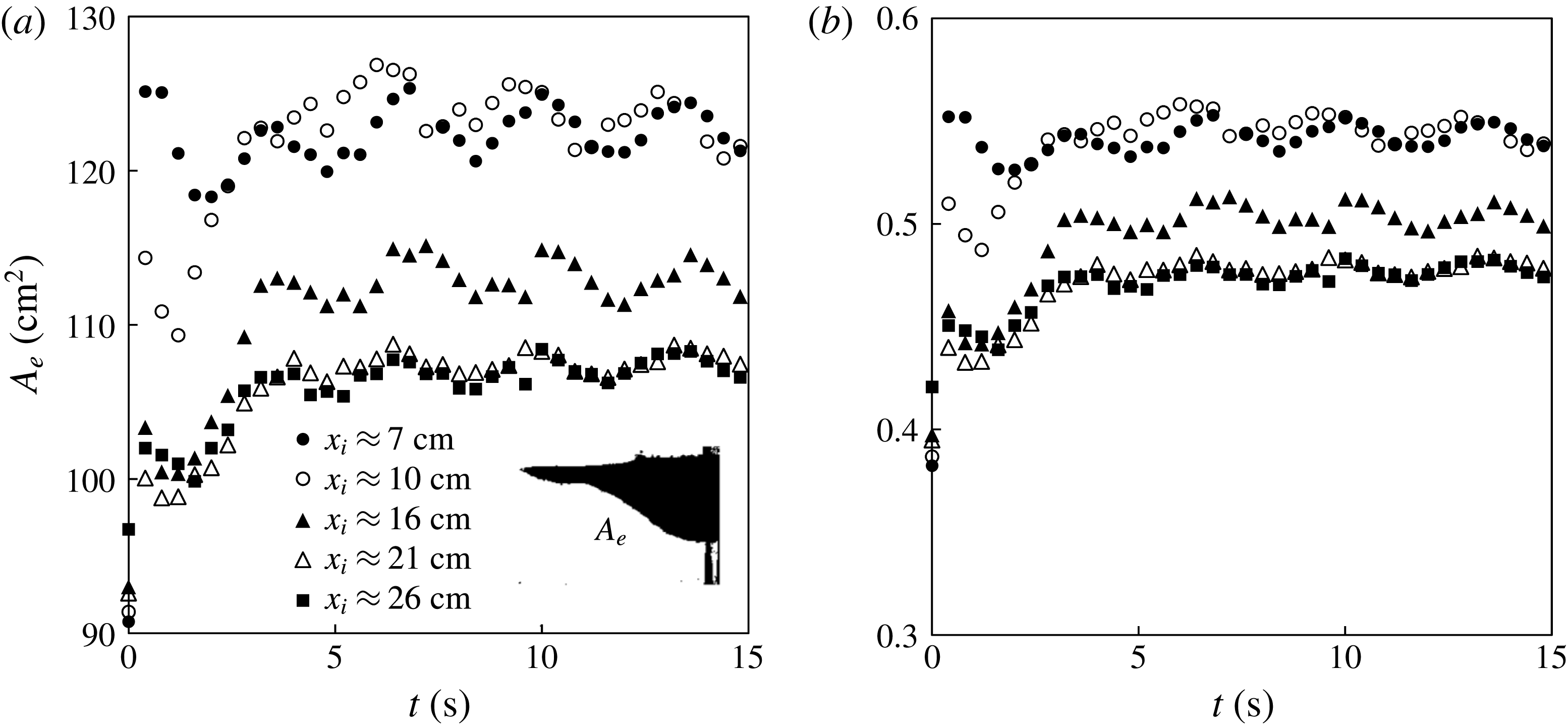
is the width of the tank. The experiments are identical to those in figure 17.

The time evolution of the intruding area
 $A_{i}(t)$
measured from the location of the lock gate
 $x_{i}$
to the front
 $x_{f}(t)$
. The definition of the intruding area is shown in the inset of (a), and the experimental results are shown in a log–log graph in (b). The experiments are identical to those in figure 17.

We show in figure 18 the incremental change of area covered by the bead layer: the blue region represents an increase in area, and the red region indicates a decrease. As time progresses, the length of the current extends, which is mainly sustained by a decrease in the thickness of the current within the lock region. The difference in the area covered by the blue and red regions indicates a porosity change for the current of beads, for which we provide a detailed calculation in this section. Eventually the front of the beads reaches a maximum location, all motion stops and the interface shape remains unchanged at later times.
First, the total area
 $A_{e}$
can be calculated from the side view pictures in representative experiments, as shown in figure 19(a). We observe an increase in
 $A_{e}$
immediately following the release of beads from the lock gate. We can then compute the effective porosity
 $\unicode[STIX]{x1D719}_{e}$
for the system of beads based on
 $\unicode[STIX]{x1D719}_{e}\equiv 1-m/(\unicode[STIX]{x1D70C}_{b}w_{t}A_{e})$
. The results are shown in figure 19(b), where we observe an increase of
 $\unicode[STIX]{x1D719}_{e}$
following the removal of the lock gate. The increase in
 $A_{e}$
and
 $\unicode[STIX]{x1D719}_{e}$
is mainly because the beads are no longer closely packed once they start to spread horizontally. In addition, based on the side view pictures, we can obtain the time evolution of the intruding area
 $A_{i}$
, measured from the location of the lock gate
 $x_{i}$
to the location of the propagating front
 $x_{f}(t)$
. The results from representative experiments are shown in figure 20, and we observe that
 $A_{i}$
first increases before gradually reaching a constant value.
We note that the thickness of beads can vary across the width of the water tank, i.e. perpendicular to the plane of the paper, which is an uncertainty in the experimental measurements. In addition, a surface wave (with an amplitude of
 ${\approx}1$
cm, for example), generated from pulling the gate out and the impact of beads, can also contribute to the experimental uncertainty. For example, the oscillations in figures 19 and 20 are likely caused by the sloshing water wave. In fact, based on long wave theory, we estimate that the water wave travels with a speed of
 $\sqrt{gd}\approx 1.2~\text{m}~\text{s}^{-1}$
. Thus, the period of the oscillations is estimated to be
 $2l_{t}/\sqrt{gd}\approx 3.4$
s, which agrees with the experimental observations.
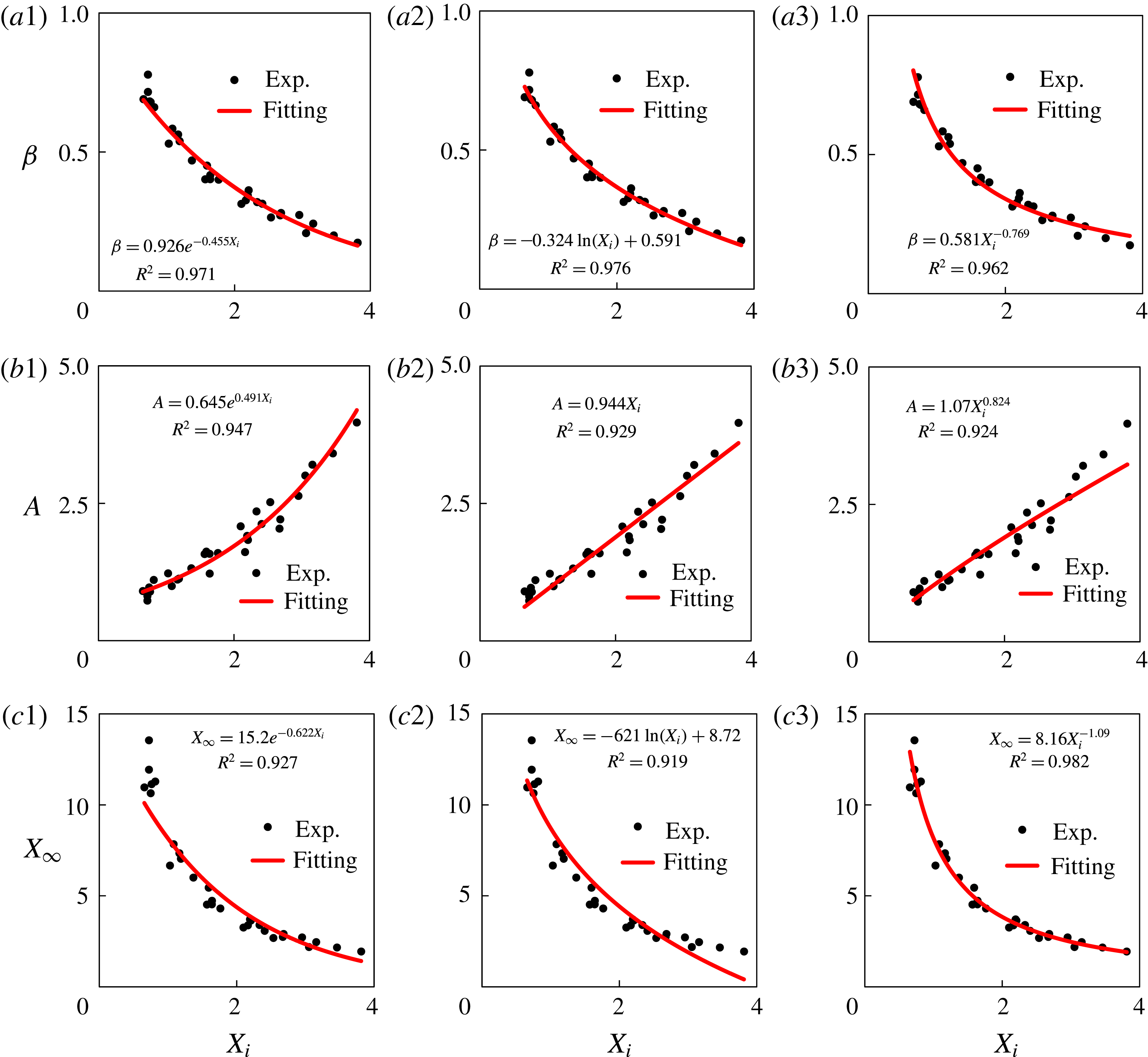
Data fitting for the experimental measurements, using different functional forms: (a1–a3) scaling exponent, (b1–b3) prefactor and (c1–c3) runout distance. The results can be used to describe the universal dynamic behaviours for the front location observed in the interfacial granular intrusion experiments.

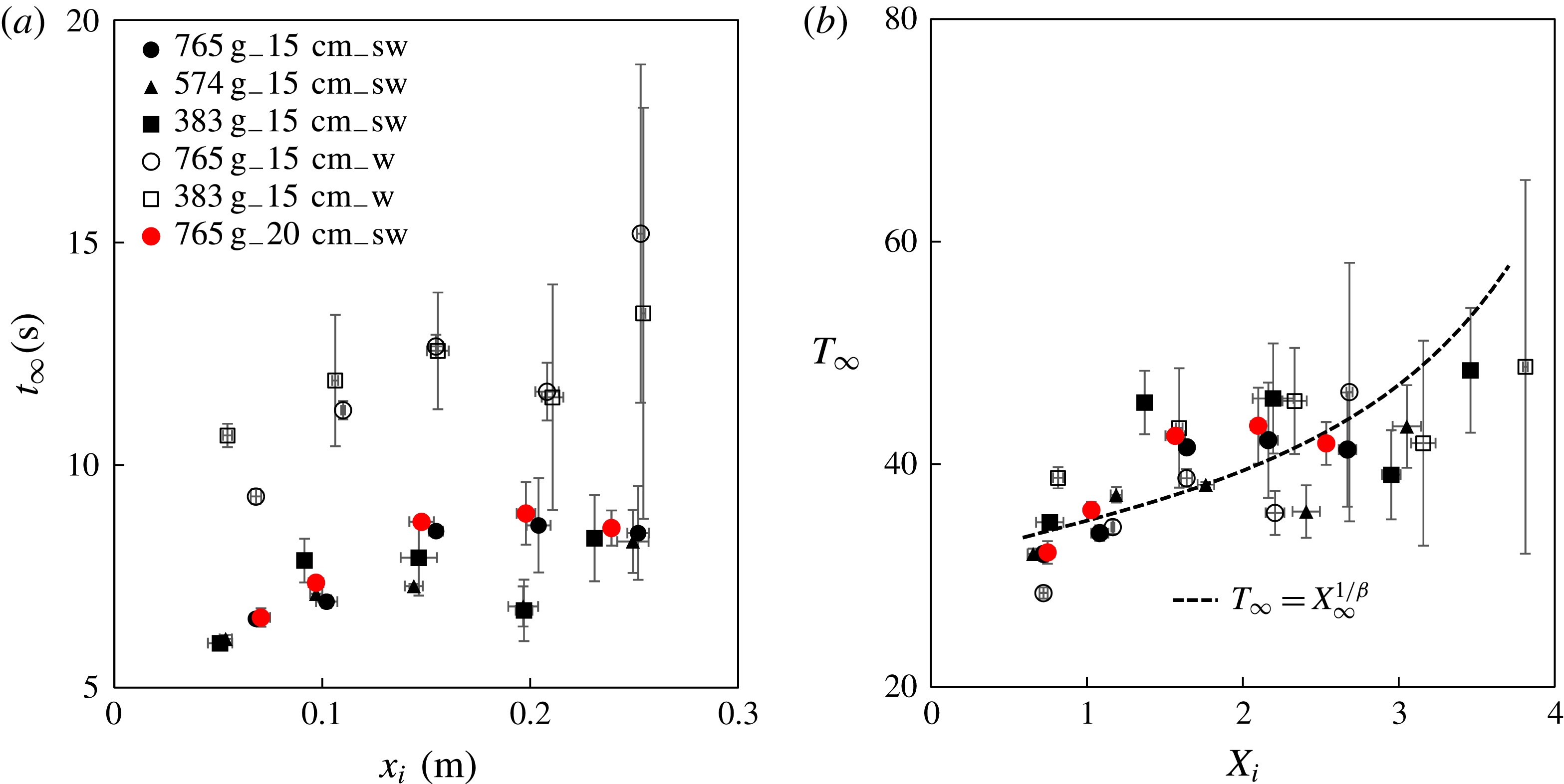
The spreading time
 $t_{\infty }$
in different experiments: (a) raw data and (b) rescaled data.
 $t_{\infty }$
is defined based on
 $x_{\infty }=\unicode[STIX]{x1D6FC}t_{\infty }^{\unicode[STIX]{x1D6FD}}$
and the dashed curve in (b) is based on (B 1b
), (B 3c
) and (C 1). The data collapse in the rescaled plot (b) and the agreement with the dashed curve further confirm that the characteristic time and length scales
 $t_{c}$
and
 $l_{c}$
, defined as (3.5) and (3.1), capture the spreading dynamics of the current of beads.

Appendix B. On experimental data fitting
We note that the experimental data can be fitted using other functional forms, besides those introduced in the main text and summarized in table 1. Here we provide more data-fitting results for the scaling exponent
 $\unicode[STIX]{x1D6FD}$
, prefactor
 $A$
, and runout distance
 $X_{\infty }$
as a function of the rescaled initial lock length
 $X_{i}$
, as also illustrated in figure 21. The results hold for
 $0.6\leqslant X_{i}\leqslant 3.8$
, as set by the experiments. We also note that some of the fitted powers are close to rational fractions.
In particular, we provide the best exponential, logarithm, and power-law fitting results for the scaling exponent
 $\unicode[STIX]{x1D6FD}$
,
 $$\begin{eqnarray}\displaystyle \unicode[STIX]{x1D6FD}=\left\{\begin{array}{@{}ll@{}}0.926\,e^{-0.455X_{i}}, & R^{2}=0.971,\\ -0.324\,\text{ln}\,X_{i}+0.591, & R^{2}=0.976,\\ 0.581\,X_{i}^{-0.769}, & R^{2}=0.962.\end{array}\right. & & \displaystyle\end{eqnarray}$$
We also provide the best exponential, linear and power-law fitting results for the dimensionless prefactor
 $A$
,
 $$\begin{eqnarray}\displaystyle A=\left\{\begin{array}{@{}ll@{}}0.645\,e^{0.491X_{i}}, & R^{2}=0.947,\\ 0.944\,X_{i}, & R^{2}=0.929,\\ 1.07\,X_{i}^{0.824}, & R^{2}=0.924.\end{array}\right. & & \displaystyle\end{eqnarray}$$
In addition, we provide the best exponential, logarithm and power-law fitting results for the dimensionless runout distance
 $X_{\infty }$
,
 $$\begin{eqnarray}\displaystyle X_{\infty }=\left\{\begin{array}{@{}ll@{}}15.2\,e^{-0.622X_{i}}, & R^{2}=0.927,\\ -6.21\,\text{ln}\,X_{i}+8.72, & R^{2}=0.919,\\ 8.16\,X_{i}^{-1.09}, & R^{2}=0.982.\end{array}\right. & & \displaystyle\end{eqnarray}$$
The data-fitting results can be used to describe the universal behaviours for the propagating front in the interfacial granular intrusion experiments.
Appendix C. On the spreading time
We investigate in this section the spreading time
 $t_{\infty }$
of the current of beads. The definition of the spreading time
 $t_{\infty }$
is given by
 $x_{\infty }=\unicode[STIX]{x1D6FC}t_{\infty }^{\unicode[STIX]{x1D6FD}}$
. Thus, once
 $\unicode[STIX]{x1D6FC}$
,
 $\unicode[STIX]{x1D6FD}$
and
 $x_{\infty }$
are identified from each experiments, the value of
 $t_{\infty }$
can be computed. The experimental data are shown in figure 22(a). The error bars are larger than those of
 $\unicode[STIX]{x1D6FC}$
,
 $\unicode[STIX]{x1D6FD}$
and
 $x_{\infty }$
, especially for fresh water experiments with a large initial lock length
 $x_{i}$
(e.g.
 $x_{i}\geqslant 15$
cm).
We can further define a dimensionless spreading time as
 $T_{\infty }\equiv t_{\infty }/t_{c}$
, where the characteristic time
 $t_{c}$
is defined by (3.5). We observe that the rescaled data collapse to a universal curve, as shown in figure 22(b), which confirms that
 $t_{c}$
correctly captures the time scale of the spreading dynamics of the granular intrusion experiments. We also note that the spreading time
 $t_{\infty }$
, based on
 $\unicode[STIX]{x1D6FC}$
,
 $\unicode[STIX]{x1D6FD}$
and
 $x_{\infty }$
and
 $T_{\infty }(X_{i})$
can be estimated by
 $$\begin{eqnarray}\displaystyle T_{\infty }=X_{\infty }^{1/\unicode[STIX]{x1D6FD}}, & & \displaystyle\end{eqnarray}$$
where
 $\unicode[STIX]{x1D6FD}(X_{i})$
and
 $X_{\infty }(X_{i})$
are provided from (B 1) and (B 3), respectively. The dashed curve in figure 22(b) is a sample calculation of
 $T_{\infty }(X_{i})$
based on (B 1b
), (B 3c
) and (C 1). The agreement with the rescaled experimental data on
 $T_{\infty }(X_{i})$
further confirms the self-consistence of the scaling arguments in this study.