2.2.1 Actuators model

At present, the actuator of the three-axis-stabilised SACS generally uses the angular momentum exchange device, which called as the wheel control system. [Reference Tu12] Considering the torque-type reaction flywheel with three-axis orthogonal fixed installation, an accurate torque balance equation needs to be introduced [Reference Chen, Zhang and Chen13], so as to describe the output torque M _m of the reaction flywheel accurately.

(1) \begin{align}{M_m} = {M_c} + {M_f} + {M_x} + {M_a} + {M_d}\end{align}

where M _c is flywheel control torque, M _f is friction torque, M _x is noise torque, M _a is aerodynamic drag torque and M _d is dynamic unbalance torque.

Briefly, the armature inductance is L, the armature resistance is R, the armature current is i(t), the opposing electromotive force is e(t), the control voltage is u(t), and the torque moment coefficient is K _m (N*m/A). The voltage balance equation of reaction flywheel can be given [Reference Chen, Zhang and Chen13]:

(2) \begin{align}\left\{ \begin{array}{l}L\dfrac{{di\left( t \right)}}{{dt}} + Ri\left( t \right) + e\left( t \right) = u\left( t \right)\\[3pt] {M_m} = {K_m}i\left( t \right)\end{array} \right.\end{align}

According to the Laplace transformation, a function relationship between the control voltage V and the motor output torque M _m is obtained.

(3) \begin{align}{M_m} = {K_m}\frac{V}{{Ls + R}}\end{align}

Based on equation (3), the simulation module in the Simulink is showed in Fig. 3.

Figure 3.

Simulation module of output torque and control voltage.

Sign the linear friction coefficient is K _l , the nonlinear friction coefficient is K _nl , the noise coefficient is K _x , the zero mean white noise is W, the aerodynamic drag coefficient is K _a and the dynamic unbalance coefficient is K _d . The function relationship between the different torque and the rotational speed Ω in the reaction flywheel [Reference Chen, Zhang and Chen13–Reference Bauer, Hong and Hughes15] is shown in equation (4):

(4) \begin{align}\left\{ \begin{array}{l}{M_f} = {K_l}\Omega + {K_{nl}}sign\left( \Omega \right)\\ \\[-7pt] {M_x} = {K_x}\left( {W/\left| {{W_{\max }}} \right|} \right)\\\\[-7pt] {M_a} = {K_a}\Omega \sqrt {\left| \Omega \right|} \\\\[-7pt] {M_d} = {K_d}{\Omega ^2}\sin \left( {\Omega t} \right)\end{array} \right.\end{align}

Based on equation (4), the functional relationship between various torque and flywheel speed can be modeled in the Simulink is showed in Fig. 4.

Figure 4.

Simulation model of torque and flywheel.

The rotational speed Ω of reaction flywheel can be integrated by the torque balance equation (14):

(5) \begin{align}\Omega = {J_c}^{ - 1}\int {{M_c}} dt\end{align}

where, J _c is the moment of inertia of reaction flywheel (kg ^* m ²).

Based on equation (5), the simulation model in the Simulink is showed in Fig. 5.

Figure 5.

Simulation model of control torque and flywheel speed.

Based on the above analysis and the reference [Reference Jiang, Wei and Cen14], the simulation model of reaction flywheel is showed in Fig. 6. Among them, the input 1 is the motor control voltage V, the output 1 is the control torque M _c of reaction flywheel, and the output 2 is the angular momentum H _a of reaction flywheel.

Figure 6.

Simulation model of reaction flywheel [Reference Jiang, Wei and Cen14].

2.2.2 Attitude dynamics model

Attitude dynamics studies the rotational motion of a satellite around its mass center under the action of external and internal torques, which not only studies the overall attitude motion of the satellite, but also studies the relative motion among various parts of the satellite [Reference Tu12]. The attitude dynamics is also related closely to the satellite structure. Regardless of the influence of the flexibility vibration, liquid fuel tank size and installation position on the attitude dynamics of the satellite, a simulation model of the attitude dynamics is established.

The dynamics equation of a satellite with flywheel can be described as follows [Reference Tu12]:

(6) \begin{align}{J_o}\dot \Omega + {J_c}\dot \omega + \omega \times \left( {{J_o}\omega + {J_c}\Omega } \right) = M\end{align}

where, J _o is the moment of inertia matrix of satellites, $\omega $ =[ $\omega $ _x $\omega $ _y $\omega $ _z ] ^T is the rotational angular velocity of satellites, M is the external torque of satellites.

The control torque M _c of reaction flywheel is ${J_c}\dot \Omega $ , so, equation (6) can be rewritten as:

(7) \begin{align}{J_o}\dot \omega + \omega \times \left( {{J_o}\omega + {J_c}\Omega } \right) = M - {M_c}\end{align}

We can integrate ${J_o}\dot \omega $ to obtain J _o $\omega $ and then multiply the inverse inv(J _o ) of moment of inertia matrix of satellite to obtain rotational angular velocity $\omega $ , and its model in the Simulink is showed in Fig. 7.

Figure 7.

Simulation model of satellite angular velocity.

The cross-multiplication of H = J _o $\omega $ + J _c Ω and the angular velocity $\omega $ can be implemented in the Simulink, the simulation model is showed in Fig. 8.

Figure 8.

Simulation model of the cross-multiplication of momentum torque and angular velocity.

Based on the above analysis and the reference [Reference Jiang, Wei and Cen14], the simulation model of attitude dynamics is showed in Fig. 9. Among them, the input 1 is the error (M-M _c ) between the external torque M and the control torque M _c , the input 2 is the momentum moment H _a of reaction flywheel, and the output 1 is the rotational angular velocity $\omega $ of the satellite.

Figure 9.

Simulation model of satellite attitude dynamics with wheel [Reference Jiang, Wei and Cen14].

2.2.3 Attitude kinematics model

When describing the change of the attitude, the method based on the quaternion only needs four parameters, and this method is no singular position; therefore, it is widely used to establish the attitude kinematics of satellites [Reference Tu12].

After the satellite rotates a certain angle around a certain axis, the Euler quaternion is defined as q =[q ₀ q ₁ q ₂ q ₃] ^T .

(8) \begin{align}\left\{ \begin{array}{l}{{q_0} = \cos \left( {\frac{\Phi }{2}} \right)} {{q_1} = {e_x}\sin \left( {\frac{\Phi }{2}} \right)} \\ {{q_2} = {e_y}\sin \left( {\frac{\Phi }{2}} \right)} {{q_3} = {e_z}\sin \left( {\frac{\Phi }{2}} \right)}\end{array} \right.\end{align}

where, $\Phi$ is the rotation angle, (e _x e _y e _z ) is the unit direction vector of rotation axis.

As ${e_x}^2 + {e_y}^2 + {e_z}^2 = 1$ , the quaternion satisfies the orthogonal constraint equation.

(9) \begin{align}{q_0}^2 + {q_1}^2 + {q_2}^2 + {q_3}^2 = 1\end{align}

The quaternion q satisfies the above constraint called normalised quaternion.

Let the satellite rotate in the order of Z-X-Y, the kinematics equation of satellite attitude based on quaternion can be described:

(10) \begin{align}\left[ {\begin{array}{c}{{{\dot q}_0}}\\ \\[-7pt]{{{\dot q}_1}}\\ \\[-7pt]{{{\dot q}_2}}\\ \\[-7pt]{{{\dot q}_3}}\end{array}} \right] = \frac{1}{2}\left[ {\begin{array}{c@{\quad}c@{\quad}c@{\quad}c}0& { - {\omega _x}}& { - {\omega _y}}& { - {\omega _z}}\\ \\[-7pt]{{\omega _x}}& 0 &{{\omega _z}} &{ - {\omega _y}}\\ \\[-7pt]{{\omega _y}} &{ - {\omega _z}} &0& {{\omega _x}}\\ \\[-7pt]{{\omega _z}} &{{\omega _y}} &{ - {\omega _1}} &0\end{array}} \right]\left[ {\begin{array}{c}{{q_0}}\\ \\[-7pt]{{q_1}}\\ \\[-7pt]{{q_2}}\\ \\[-7pt]{{q_3}}\end{array}} \right]\end{align}

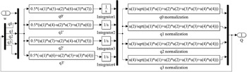
Taking the attitude angular velocity and quaternion as input, the current attitude quaternion can be obtained through integration and regularisation. According to equations (9), (10) and reference [Reference Zhang16], the simulation model of attitude kinematics based on quaternion in the Simulink is showed in Fig. 10.

Figure 10.

Simulation model of attitude kinematics based on quaternion.

The attitude matrix can be used to convert the attitude quaternion into the attitude Euler angle. The attitude matrix based on quaternion can be given [Reference Tu12]

(11) \begin{align}A = \left[ {\begin{array}{c@{\quad}c@{\quad}c}{{q_0}^2 + {q_1}^2 - {q_2}^2 - {q_3}^2} & {2\left( {{q_1}{q_2} + {q_3}{q_0}} \right)}& {2\left( {{q_1}{q_3} - {q_2}{q_0}} \right)}\\ \\[-7pt]{2\left( {{q_1}{q_2} - {q_3}{q_0}} \right)} &{{q_0}^2 - {q_1}^2 + {q_2}^2 - {q_3}^2} &{2\left( {{q_2}{q_3} + {q_1}{q_0}} \right)}\\ \\[-7pt]{2\left( {{q_1}{q_3} + {q_2}{q_0}} \right)} &{2\left( {{q_2}{q_3} - {q_1}{q_0}} \right)} &{{q_0}^2 - {q_1}^2 - {q_2}^2 + {q_3}^2}\end{array}} \right]\end{align}

Based on equation (11) and reference [Reference Zhang16], the simulation model of attitude matrix in the Simulink is showed in Fig. 11.

Figure 11.

Simulation model of attitude matrix based on quaternion.

The functional relationship between the attitude matrix and the attitude angle can be given [Reference Tu12]:

(12) \begin{align}\left[ {\begin{array}{c}\varphi \\ \\[-7pt]\theta \\ \\[-7pt]\psi \end{array}} \right] = \left[ {\begin{array}{c}{arct{g_2}\left( {2\left( {{q_0}{q_1} + {q_2}{q_3}} \right),1 - 2\left( {{q_1}^2 + {q_2}^2} \right)} \right)}\\ \\[-7pt]{\arcsin \left( {2\left( {{q_0}{q_2} - {q_3}{q_1}} \right)} \right)}\\ \\[-7pt]{arct{g_2}\left( {2\left( {{q_0}{q_3} + {q_1}{q_2}} \right),1 - 2\left( {{q_2}^2 + {q_3}^2} \right)} \right)}\end{array}} \right]\end{align}

Based on equation (12) and reference [Reference Zhang16], the simulation model in the Simulink is showed in Fig. 12.

Figure 12.

Simulation model of attitude angle based on quaternion.

Based on the above analysis, we take the attitude angular velocity as the input and establish the simulation model of attitude kinematics based on quaternion, so as to calculate the attitude angle. The simulation model is showed in Fig. 13.

Figure 13.

Simulation model of attitude angle solving based on quaternion.

2.2.4 Gyroscopes model

The three-rate integral gyros are used to measure the angular velocity of the satellite, which are parallel to the three axes of the satellite and are installed orthogonally to each other. The measurement model of the gyroscope can be given [Reference Bian, Cheng and Xue17, Reference Zhu and Li18]:

(13) \begin{align}\left\{ \begin{array}{c}{\omega _g} = \omega + b + d + {n_g}\\ \\[-7pt] \dot d = - Dd + {n_d}\end{array} \right.\end{align}

where, $\omega $ _g is the measured angular velocity of gyros, b is the constant drifting of gyros, n _g is the measured noise of gyros, d is the random drifting of gyros, n _d is the noise of random drifting and D=diag(1/τ _x 1/τ _y 1/τ _z ) is the diagonal matrix formed by the correlation time constant τ _i (i = x,y,z).

Based on equation (13), the simulation model in the Simulink is showed in Fig. 14. Among them, the input 1 is the angular velocity $\omega $ of the satellite, and the output 1 is the measured angular velocity $\omega $ _g of the gyros.

Figure 14.

Simulation model of the gyros [Reference Jiang, Wei and Cen14].

2.2.5 Earth sensors model

The earth sensors are used to measure the attitude angles of the satellite. The two earth sensors have been adopted to measure the roll angle $\varphi $ and pitch angle θ of the satellite. The measured model of earth sensors can be given [Reference Yang, Yu and Miao19, Reference Wang, Xing and You20]

(14) \begin{align}\left\{ \begin{array}{c}{\varphi _e} = \varphi + {\varphi _b} + {\varphi _n}\\ \\[-7pt] {\theta _e} = \theta + {\theta _b} + {\theta _n}\end{array} \right.\end{align}

where, $\varphi $ _e and θ _e is the measured output of earth sensors, $\varphi $ _b and θ _b is the constant deviation of earth sensors, $\varphi $ _n and θ _n is the measured noise of earth sensors.

Based on equation (14), the simulation model in the Simulink is showed in Fig. 15. Among them, the input 1 is the $\varphi $ and θ of the satellite, the output 1 is the measured angle $\varphi $ _e and θ _e of earth sensors.

Figure 15.

Simulation model of the earth sensor [Reference Jiang, Wei and Cen14].

2.2.6 Attitude determination model

According to the principle of the attitude determination based on the gyroscope and the earth sensor, and the design method of the state observer in modern control theory [Reference Tu12], the estimation value $( {\hat \varphi }\ {\hat \theta }\ {\hat \psi })$ of the roll, pitch and yaw angle can be obtained:

(15) \begin{align}\left\{ \begin{array}{l}\dot{\hat{\varphi}} = {\omega _o}\hat \psi + {\omega _{gx}} + {K_\varphi }( {{\varphi _m} - \hat \varphi })\\\dot{\hat{\theta}} = {\omega _o} + {\omega _{gy}} + {K_\theta }( {{\theta _m} - \hat \theta } )\\\dot{\hat{\psi}} = - {\omega _o}\hat \varphi + {\omega _{gz}} + {K_\psi }( {{\varphi _m} - \hat \varphi } )\end{array} \right.\end{align}

where, $( {\dot{\hat{\varphi}}}\ {\dot{\hat{\theta}} }\ {\dot{\hat{\psi}} })$ is the estimation value of attitude angular velocity, $\omega $ _o is the instantaneous angular velocity of the satellite, (K $_{\varphi} $ K $\theta $ K $\psi $ ) is the gain coefficient and its value is 0.005 $\sim $ 0.05(1/s).

Based on equation (15), the simulation model of the attitude determination in the Simulink is showed in Fig. 16. Among them, the input 1 is the measured angle $\varphi $ _e and θ _e of earth sensors, the input 2 is the measured angular velocity $\omega $ _g of gyroscopes, the output 1 is the estimation value $( {\hat \varphi }\ {\hat \theta }\ {\hat \psi } )$ of attitude angles, the output 2 is the estimation value $( {\dot{\hat{\varphi}} }\ {\dot{\hat{\theta}} }\ {\dot{\hat{\psi}} } )$ of attitude angular velocity.

Figure 16.

Simulation model of attitude determination [Reference Jiang, Wei and Cen14]‘.

The conversion relationship between the attitude Euler angle and the quaternion is as follows.

(16) \begin{align}q = \left[ \begin{array}{c} {{q_0}} \\ \\[-9pt] {{q_1}} \\ \\[-9pt] {{q_2}} \\ \\[-9pt] {{q_3}} \\ \\[-9pt] \end{array} \right] = \left[ \begin{array}{c} {\cos (\varphi /2)\cos (\theta /2)\cos (\psi /2) + \sin (\varphi /2)\sin (\theta /2)\sin (\psi /2)} \\ \\[-9pt] {\sin (\varphi /2)\cos (\theta /2)\cos (\psi /2) - \cos (\varphi /2)\sin (\theta /2)\sin (\psi /2)} \\ \\[-9pt] {\cos (\varphi /2)\sin (\theta /2)\cos (\psi /2) + \sin (\varphi /2)\cos (\theta /2)\sin (\psi /2)} \\ \\[-9pt] {\cos (\varphi /2)\cos (\theta /2)\sin (\psi /2) - \sin (\varphi /2)\sin (\theta /2)\cos (\psi /2)} \\ \\[-9pt] \end{array} \right]\end{align}

Based on equation (16), the simulation model in the Simulink is showed in Fig. 17.

Figure 17.

Simulation model of attitude quaternion solving.

2.2.7 Controller model

Assuming that the current quaternion is Q , the desired attitude quaternion is Q _d , the error quaternion Q _e can be expressed as [Reference Han21]

(17) \begin{align}{Q_e} &= {Q_d}^*Q\nonumber\\[3pt] &= \left[ {\begin{array}{c}{{q_{d0}}{q_0} - {q_d}^Tq}\\ \\[-7pt]{{q_d}{q_0} + {q_{d0}}q + {q_d} \times q}\end{array}} \right]\end{align}

where, Q _d *=[q _d0 - q _d ] ^T and Q =[q ₀ q ] ^T .

Based on equation (17), the simulation model in the Simulink is showed in Fig. 18.

Figure 18.

Simulation model of error quaternion.

In order to quickly capture the dynamic performances of the attitude changes and enable the satellite attitude to quickly stabilise to the desired position, we choose the PD controller [Reference Schwabacher22]. The error quaternion and error angular velocity are used as the control variables, and the control law is designed.

(18) \begin{align}u = - {K_p}{q_e} - {K_d}{\omega _e}\end{align}

where, K _p and K _d are the control coefficients.

Based on the above analysis, the simulation model of PD controller in the Simulink is showed in Fig. 19. Among them, the input 1 is the error attitude angular velocity $\omega $ _e , the input 2 is the error attitude quaternion q _e , and the output 1 is the control voltage V.

Figure 19.

Simulation model of PD controller.

Therefore, a complete simulation platform of the SACS is showed in Fig. 20.

Figure 20.

Simulation platform of the SACS.

3.2.1 Simulation analysis of controller faults

Assuming that the intermittent fault appears the controller output between 7 to 8 seconds, the simulation results are showed in Fig. 27. It can be seen that the intermittent faults of the controller will result in a longer response time to reach stability.

Figure 27.

Simulation results of the controller under intermittent faults.

If the mutations faults appear the controller output at the 7s, the simulation results are showed in Fig. 28. It can be seen that when the mutation faults appear the controller, the output torque of the reaction flywheel fluctuates greatly, the angular velocity tends to stable after a long time, but there is a large deviation from the expected value, the attitude angle will exhibit a periodic change. The simulation results indicate that the mutations faults of the controller can degrade the performance of the SACS.

Figure 28.

Simulation results of the controller under mutation faults.

3.2.2 Simulation analysis of actuator faults

Since each of the three axes of the satellite is equipped with a reaction flywheel, the faults may occur on the reaction flywheel at different positions. Therefore, the simulation analysis of the impact of the faults of the single reaction flywheel and the combined reaction flywheel on the system performance are done in this section.

3.2.2.1 Fault impact of single reaction flywheel

Assuming that the multiplicative fault appears the reaction flywheel 3, the simulation results of attitude angular velocity and angle are showed in Fig. 29. It can be seen that the angular velocity and attitude angle will eventually change irregularly and not be stable anymore, which indicates that the multiplicative faults of the reaction flywheel damage the stability of the SACS.

Figure 29.

Simulation results of the reaction flywheel 3 under multiplicative faults.

If the stuck fault appears the reaction flywheel 3, the simulation results of attitude angular velocity and angle are showed in Fig. 30.

Figure 30.

Simulation results of the reaction flywheel 3 under stuck faults.

From Fig. 30, it can be seen that when the stuck faults appears on the reaction flywheel, the stability of the SACS is destroyed and the system cannot be stabilized.

3.2.2.2 Fault impact of combined reaction flywheel

The impact of single reaction flywheel fault on system performance has been simulated and analysed. Next, we will analyse the simulation results of the impact of combined reaction flywheel fault on system performance. The specific combination method and simulation results are as follows.

When the fault occur on the reaction flywheel 1 and 2 at the same time, the simulation results of the attitude angular velocity and angle are showed in Fig. 31. It can be seen that the angular velocity on the X axis gradually decreases, and the angular velocity on the Z and Y axes always presents an oscillating form with a large deviation; the attitude angle is always oscillating and is difficult to maintain stable. The simulation results indicate that the stability of the system is undermined.

Figure 31.

Simulation results of the reaction flywheel 1 and 2 faults simultaneously.

When the fault occur on the reaction flywheel 1 and 3 at the same time, the simulation results of the attitude angular velocity and angle are showed in Fig. 32. It can be seen that the angular velocity tends to stabilise after a long time; the deviation of the attitude angle will gradually increase. The simulation results indicate that the stability of the system will become worse and worse.

Figure 32.

Simulation results of the reaction flywheel 1 and 3 faults simultaneously.

When the fault occur on the reaction flywheel 2 and 3 at the same time, the simulation results of the attitude angular velocity and angle are showed in Fig. 33. It can be seen that the angular velocity on the X axis gradually increases, and the angular velocity on the Y and Z axes always presents an oscillating form with a large deviation; the attitude angle is constantly oscillating and is difficult to maintain stability. The simulation results indicate that the stability of the system has been damaged.

Figure 33.

Simulation results of the reaction flywheel 2 and 3 faults simultaneously.

When the fault occur on the three reaction flywheels at the same time, the simulation results of the attitude angular velocity and angle are showed in Fig. 34. It can be seen that the angular velocity on the X and Y axes presents a divergent oscillation, and the angular velocity on the Z axis will eventually stabilise, but the deviation very large; the attitude angle has been oscillating and is difficult to maintain stability. The simulation results indicate that the stability of the system has been damaged.

Figure 34.

Simulation results of the three reaction flywheel faults simultaneously.

3.2.3 Simulation analysis of attitude sensors faults

In this paper, the attitude sensor includes gyroscopes and earth sensors. When the gyroscope occurs graded faults and the earth sensor is normal, the simulation results of the attitude angular velocity and angle are showed in Fig. 35. It can be seen that the gradual faults of the gyroscope will cause the deviation of the angular velocity to increase, and the attitude angle will show a small amplitude periodic oscillation, which will affect the stability of the system.

Figure 35.

Simulation results of gyroscope under graded faults.

When the earth sensor occurs the graded faults and the gyroscope is normal, the simulation results of the attitude angular velocity and angle are showed in Fig. 36. It can be seen that the gradual faults of the earth sensor will cause a cumulative deviation in the attitude angle, which will affect the stability of the system.

Figure 36.

Simulation results of earth sensor under graded faults.

When the gyroscope and earth sensor occur the graded faults at the same time, the simulation results of the attitude angular velocity and angle are showed in Fig. 37. It can be seen that the gradual faults of the gyroscope and the earth sensor will cause the deviation of the angular velocity to increase, and the attitude angle will show a small amplitude periodic oscillation, which will affect the stability of the system.

Figure 37.

Simulation results of gyroscope and earth sensor under graded faults.

3.2.4 Simulation analysis of measurement noise

There is measurement noise in the measurement components. We have carried out the simulation analysis of the influence of measurement noise on attitude angular velocity and angle. The simulation results are showed in the Figs 38-39. It can be seen that measurement noise will affect the attitude angular velocity and angle. The greater the measurement noise, the greater the deviation of the attitude angular velocity and angle.

Figure 38.

Simulation results of measurement noise under 10σ.

Figure 39.

Simulation results of measurement noise under 50σ.

In summary, the component faults and the measurement noise can affect the performance of the SACS and even destroy the stability of the system, and the simulation result shows that the designed simulation platform can well simulate the impact of system faults on the performance of the SACS.