





1. Introduction
1.1. Context
Understanding the fluid dynamics of viscoelastic suspensions is of great interest both for optimising industrial processes and for advancing the understanding of complex fluids used across diverse fields. These materials, which exhibit a combination of viscous and elastic properties, play a crucial role in applications ranging from paints (Osterhold Reference Osterhold2000) and foods (Moelants et al. Reference Moelants, Cardinaels, Van Buggenhout, Van Loey, Moldenaers and Hendrickx2014) to fracking fluids (Liu et al. Reference Liu, Li, Zhao, Liu and Liu2021) and biological suspensions (Brust et al. Reference Brust, Schaefer, Doerr, Pan, Garcia, Arratia and Wagner2013). In the food industry, for instance, viscoelasticity enhances product texture, stability and shelf life. Fracking fluids exploit these properties to more effectively fracture rock formations, while biological suspensions used in pharmaceuticals and biomedical applications require precise control over their viscoelastic response. In the context of the energy transition, improving operational speeds and overall process efficiency remains a major challenge for industrial stakeholders. Many industrial operations involve the flow of liquid materials in which energy, momentum or species must be transported and transferred. While modifying geometry or structural configurations (akin to adaptations observed in natural systems, Bushnell & Moore Reference Bushnell and Moore1991) often provides the most direct route to efficiency gains, an increasingly attractive alternative lies in tailoring the rheological behaviour of the working fluid itself. In that context, the present paper places emphasis on viscoelastic suspensions that consist of solid particles suspended in a viscoelastic base fluid.
It is well established that adding a small fraction of polymer to a Newtonian base fluid can significantly reduce drag in shear flows (Lumley Reference Lumley1973; Serafini Reference Serafini2022). This effect arises from the viscoelastic behaviour altering the turbulent kinetic energy cascade and/or introducing new pathways to turbulence (Steinberg Reference Steinberg2021; Boulafentis et al. Reference Boulafentis, Lacassagne, Cagney and Balabani2023; Dubief et al. Reference Dubief, Terrapon and Hof2023; Moazzen et al. Reference Moazzen, Lacassagne, Thomy and Bahrani2023; Song et al. Reference Song, Zhu, Lin, Liu and Khomami2023), where fluid elasticity modifies both the onset of instabilities and the mechanisms of transition. In particular, elastic turbulence (Steinberg Reference Steinberg2021) and its elasto-inertial counterpart illustrate how polymer-induced stresses reshape turbulence dynamics. Elasto-inertial turbulence (EIT) is observed at Reynolds numbers,
 $\mathcal{R}$
, that are significantly lower than those required for the onset of inertial turbulence in Newtonian fluids;
 $\mathcal{R}$
is defined in (1.1) for the present Taylor–Couette flow context. At the same time, it occurs at high Weissenberg numbers,
 $\mathcal{W}$
(also defined in (1.1)), which quantify the strength of elastic stresses. This regime of turbulence emerges from nonlinear interactions between polymer-generated elastic forces and fluid inertia (Dubief et al. Reference Dubief, Terrapon and Hof2023)
 \begin{align} \mathcal{R} = \frac {\rho r_i \varOmega \delta }{\mu } = \frac {\rho \dot {\gamma } \delta ^2}{\mu }, \quad \mathcal{W} = \lambda \dot {\gamma }, \quad \mathcal{E} = \frac {\mathcal{W}}{\mathcal{R}} = \frac {\lambda \mu }{\rho \delta ^2} ,\end{align}
where
 $\mathcal{R}, \mathcal{W}$
and the elastic number (
 $\mathcal{E}$
) are three dimensionless numbers frequently used in elasto-inertial transitions studies where
 $\rho$
is the fluid density in
 $\textrm{kg}\,\textrm{m}^{-3}$
,
 $\mu$
the fluid shear viscosity in
 $\textrm{Pa}\,\textrm{s}$
and
 $\lambda$
the elastic relaxation time of the solution in
 $s$
. In the Taylor–Couette context of this work,
 $r_i$
is the inner cylinder radius in
 $\textrm{m}$
,
 $\varOmega$
the inner cylinder rotational speed in
 $\textrm{s}^{-1}$
,
 $\delta$
the gap between outer and inner cylinders in
 $\textrm{m}$
and
 $\dot {\gamma }=\varOmega r_i/\delta$
the resulting shear rate in
 $\textrm{s}^{-1}$
. These dimensionless numbers are presented here, as they are reported for this study in table 2, to help the reader place the present work in the context of the literature.
While the combination of an early chaotic dynamics at low inertia and flow rates, together with the tuneable drag properties introduced by viscoelasticity and elasto-inertial effects, holds considerable promise for industrial applications, another strategy for process intensification is to modify fluid properties by dispersing solid particles into the liquid solvent. This approach enables the tailoring of physical properties such as thermal capacity or conductivity. It has driven substantial interest in the study of nanofluids (Khanafer & Vafai Reference Khanafer and Vafai2011; Briclot et al. Reference Briclot, Henry, Popa, Nguyen and Fohanno2020), where metallic nanoparticles suspended at dilute to moderate volume fractions have been shown to enhance heat transfer performance, albeit at the cost of increased pressure drops. However, due to growing health and environmental concerns associated with nanoparticles, recent research efforts have increasingly shifted towards the use of microparticles.
The primary effect of adding (micro- or nano-) particles to a liquid phase is an increase in viscosity (Einstein Reference Einstein1906; Wildemuth & Williams Reference Wildemuth and Williams1984), which at sufficiently high concentrations can lead to non-Newtonian rheological behaviour (Vázquez-Quesada et al. Reference Vázquez-Quesada, Tanner and Ellero2016). In the case of microparticles, however, it has been shown that solid inclusions, even when neutrally buoyant, can promote convective instabilities (Morris Reference Morris2020), and modify the transition to turbulence by altering the nature of the primary instability and reshaping the signatures of higher-order modes, particularly in centrifugal flows and Taylor–Couette configurations (Majji et al. Reference Majji, Banerjee and Morris2018; Ramesh et al. Reference Ramesh, Bharadwaj and Alam2019; Dash et al. Reference Dash, Anantharaman and Poelma2020; Moazzen Reference Moazzen2022; Kang et al. Reference Kang, Schatz and Mirbod2024).
While the particle- and viscoelasticity-related effects discussed above hold significant promise for process intensification, the underlying physical mechanisms remain only partially understood – both when considered separately and, even more so, when acting in combination. A summary of the current understanding of these complex viscoelastic suspensions is provided in the following paragraphs.
1.2. Current understanding of viscoelastic suspensions
A central aspect of the flow dynamics in such fluids is their rheology, which arises from the complex interactions between solid particles and the polymer matrix. In recent years, numerous studies have examined how local interaction mechanisms between polymer chains and particles influence both apparent rheological properties (e.g. viscosity, normal stress differences, extensional viscosity; Tanner Reference Tanner2019) and macroscopic behaviours such as particle migration (D’Avino et al. Reference D’Avino, Greco and Maffettone2017) or polymer degradation. These developments are summarised below.
1.2.1. Particle contribution to stress
In a dilute suspension (as defined by a particle volume fraction
 $\varPhi \lt 1\,\%$
), the particles do not interact directly with each other, but only with the neighbouring fluid. The latter exerts a pressure on the particle which, due to its non-deformability, returns this pressure to the fluid: the ‘stresslet’ (Morris Reference Morris2020). As particle concentration increases (
 $\varPhi \gt 1\,\%$
), the distance between particles decreases and inter-particle and the flow perturbation/stresslet caused by individual particles begin to overlap: this defines the semi-dilute regime. Ultimately, at even larger particle concentration, interparticle collisions become significant. This leads to exchanges of momentum, energy dissipation and, potentially, particle agglomeration (Marchioli et al. Reference Marchioli2025).
Unlike the stresslet, which only describes the interaction between a particle and the surrounding fluid (via the action–reaction law, since the particle is not deformable), an additional stress arises when the fluid is perturbed by the stresses imposed by the presence of particles. This contribution, known as the particle-induced fluid stress (PIFS), reflects the local modification of the flow (Jain et al. Reference Jain, Einarsson and Shaqfeh2019; Jain & Shaqfeh Reference Jain and Shaqfeh2021; Zhang & Shaqfeh Reference Zhang and Shaqfeh2023) and, in complex suspensions, accounts for the viscoelastic component of the response. In pure shear flow, the contribution of PIFS to the apparent viscosity has been shown to increase monotonically with fluid elasticity, even while the overall stress may decrease. This phenomenon leads to apparent shear thickening in viscoelastic suspensions upon particle addition (Guido & Shaqfeh Reference Guido and Shaqfeh2019).
Numerical simulations by Matsuoka et al. (Reference Matsuoka, Nakayama and Kajiwara2021) provide further insight into this mechanism in simple shear flow. Their results show that the local shear gradient not only intensifies but also shifts spatially with increasing particle concentration, highlighting the amplification of local gradients in the fluid. At low Weissenberg numbers, elastic effects remain negligible because the fluid relaxes the limited stored energy faster than the imposed deformation time scale, thereby preventing a significant elastic ‘memory’ effect. Their analysis also reveals that, at very low concentrations (
 $\varPhi \simeq 0.1\,\%$
), local shear is highly heterogeneous and concentrated near particle surfaces, whereas at higher concentrations it becomes more uniformly distributed. Three key pieces of local information thus emerge, providing a clearer understanding of the hydrodynamic impact of particles in a viscoelastic fluid: (i) the state of deformation (uniaxial or biaxial elongation), (ii) the vorticity field around the particles and (iii) the stretching of polymer chains, which is strongly correlated with local elastic stresses. The results show that significant polymer stretching develops at concentrations above
 $\varPhi \simeq 10\,\%$
and at larger
 $\mathcal{W}$
, particularly upstream and downstream of the particles. In this regime, elastic stresses acquire a collective character: they extend throughout the fluid rather than remaining confined near individual particles. This suggests the emergence of a network of interconnected elastic stresses, resulting in superimposed local stress fields.
Such a mechanism can be interpreted as a form of local shear thickening or strain hardening. However, in contrast to Newtonian suspensions – where thickening typically arises from particle collisions or microstructural arrangements – here, it originates from the intrinsic elastic response of the polymer matrix, amplified by hydrodynamic perturbations induced by the particles. Figure 1 conceptually illustrates the interactions between particles and polymers in a viscoelastic suspension as functions of
 $\mathcal{W}$
and the particle volume fraction
 $\varPhi$
.
Conceptual representation of stresses and interactions between particles and polymers in viscoelastic suspensions in shear flow.

Figure 1. Long description
A conceptual representation of stresses and interactions between particles and polymers in viscoelastic suspensions in shear flow. The diagram includes two main parts: a stresslet and a particle interaction flow structure (PIFS). In the stresslet, fluid pressure and particle reaction are depicted with arrows pointing towards and away from a central particle, respectively. The PIFS shows multiple particles connected by polymer chains, with elongated polymer chains indicated by spring-like structures. The diagram illustrates the interaction between these components under shear flow, highlighting the viscoelastic properties of the suspension. The stresslet and PIFS are labeled, and the direction of shear flow is indicated by arrows. The overall structure emphasizes the dynamic interactions and stresses within the viscoelastic suspension.
1.2.2. Local shear thickening, strain hardening
As discussed above, competition between the various fluid transport and relaxation mechanisms can lead to marked shear thickening when fluid elasticity is non-negligible (Einarsson et al. Reference Einarsson, Yang and Shaqfeh2018; Matsuoka et al. Reference Matsuoka, Nakayama and Kajiwara2021). This phenomenon, known as elastic strain hardening, manifests itself as an increase in apparent viscosity as a function of the Weissenberg number, even in dilute suspensions. To account for this behaviour, Einarsson et al. (Reference Einarsson, Yang and Shaqfeh2018) generalised the classical Einstein model, which predicts the effective viscosity of dilute suspensions in a Newtonian fluid, to viscoelastic fluids, taking into account the relative contribution of the polymer to viscosity and the effect of elasticity (via the
 $\mathcal{W}^2$
term in (1.3)). The shear viscosity is expressed as
 \begin{align} \mu =1+2.5\varPhi +(0.62-0.03\mu _r)\varPhi \mu _r \mathcal{W}^2 , \\[-28pt] \nonumber \end{align}
 \begin{align} \mu _r=\mu _p/(\mu _s+\mu _p) , \\[0pt] \nonumber \end{align}
where
 $\mu _r$
,
 $\mu _p$
and
 $\mu _s$
are the relative viscosity, the contribution of the polymer to the viscosity and the solvent viscosity in
 $\textrm{Pa}\,\textrm{s}$
.
One may note that this shear thickening is also observed numerically for normal stresses (Scirocco et al. Reference Scirocco, Vermant and Mewis2005; Yang & Shaqfeh Reference Yang and Shaqfeh2018; Jain et al. Reference Jain, Einarsson and Shaqfeh2019). More recently, Matsuoka et al. (Reference Matsuoka, Nakayama and Kajiwara2021) refined this model by breaking down the microscopic contributions to viscosity, distinguishing between stresslet (the particle’s mechanical resistance to shear) ((1.5)) and PIFS ((1.6)), i.e. the elastic stress generated in the fluid by the particle-induced disturbance
 \begin{align} \mu =1+2.5\varPhi +\varPhi \mu _r (\alpha _{\textit{stresslet}} + \alpha _{\textit{PIFS}}) , \\[-28pt] \nonumber \end{align}
 \begin{align} \alpha _{\textit{stresslet}} = -1.43\mathcal{W}^2 -0.06\mu _r\mathcal{W}^2 , \\[-28pt] \nonumber \end{align}
 \begin{align} \alpha _{\textit{PIFS}}=2.05\mathcal{W}^2+0.03\mu _r\mathcal{W}^2 . \\[0pt] \nonumber \end{align}
This result is essential, as it highlights two opposing effects: the contribution of the stresslet tends to reduce viscosity (shear thinning with increasing particles volume fraction), while the PIFS, on the other hand, accentuates thickening. This latter effect directly reflects the fluid’s elastic response to particle-induced hydrodynamic perturbations, and forms the core of the strain hardening mechanism observed.
1.2.3. Shear-induced migration in viscoelastic media
Beyond those macroscopic constitutive equation approaches considering the suspension as a single phase fluid, one should mention another remarkable fluid–particle interaction mechanism arising in viscoelastic suspensions: the viscoelasticity-induced migration of particles in confined flows. Particles can travel normal to the main direction of flow towards the nearest wall if confinement and viscoelasticity are present, as studied and reviewed by D’Avino et al. (Reference D’Avino, Maffettone, Greco and Hulsen2010, Reference D’Avino, Snijkers, Pasquino, Hulsen, Greco, Maffettone and Vermant2012). It has been shown that, in a viscoelastic fluid, particles tend to align to form particle chains under the effect of shear (Scirocco et al. Reference Scirocco, Vermant and Mewis2004). This effect seems to be amplified when the suspending fluid is shear thinning, where viscosity decreases nonlinearly with the shear rate due to the reorganisation of the fluid’s internal structures, thus reducing viscous dissipation. However, the effects of particle migration due to viscosity stratification are less pronounced when the suspending fluid is Boger (fluid with constant viscosity over a wide shear range). In this case, it is necessary to shear the suspension for very long periods or reach higher Weissenberg number values to observe migration (Pasquino et al. Reference Pasquino, Snijkers, Grizzuti and Vermant2010). These particle migration effects have been studied experimentally and theoretically but, to the best of the authors’ knowledge, only in isolated particle cases or in the dilute regime. The question of particle migration in a viscoelastic matrix in the semi-dilute regime remains to be explored, but would be expected to have a significant impact on hydrodynamic transitions, akin what was observed for inertial or shear-induced migration in particle-laden Newtonian fluids (Baroudi et al. Reference Baroudi, Majji and Morris2020, Reference Baroudi, Majji, Peluso and Morris2023).
1.2.4. Polymer degradation phenomena
From a more practical standpoint, polymer degradation plays a central role in understanding the dynamic behaviour of viscoelastic suspensions, and it is reasonable to assume that this process may be influenced by the presence of solid particles. While polymer chains can undergo scission due to photochemical, thermal or oxidative effects (Vohlídal Reference Vohlídal2021), mechanical degradation remains the dominant pathway when the fluid is chemically stable and temperature is controlled. In flow, velocity gradients stretch polymer chains: segments near the chain centre experience the highest extension and may rupture if shear rates are sufficiently high, while the terminal segments tend to remain coiled. As a result, maximum strain typically localises near the chain midpoint (Barth & Carlin Jr. Reference Barth and Carlin1984). Conversely, the long-term ageing of polymers in very low-shear flows can also lead to gradual scission (Brennen & Gadd Reference Brennen and Gadd1967), an effect that intensifies with increasing polymer concentration. Moreover, polymers dissolved in good solvents, where chains adopt more extended conformations, exhibit greater sensitivity to shear-induced degradation than those in more coiled states.
Two main theoretical frameworks have been proposed to describe the relationship between shear degradation and molecular weight (Barth & Carlin Jr. Reference Barth and Carlin1984). The first posits the existence of a limiting molecular weight: once polymer chains reach this critical length, no further scission occurs, as chains adapt to applied stress by moving within their solvent sheath rather than breaking primary bonds (Abdel-Alim & Hamielec Reference Abdel-Alim and Hamielec1973). The second theory argues that no such critical threshold exists; instead, the probability of chain scission decreases progressively with decreasing molecular weight (Rodriguez & Winding Reference Rodriguez and Winding1959).
1.3. Taylor–Couette flow of viscoelastic suspensions
As discussed in § 1.2, the interplay between viscous and elastic components in viscoelastic suspensions gives rise to complex behaviours that remain incompletely understood. Advancing our understanding of such suspensions is therefore essential, both for developing theoretical frameworks and for improving practical applications across scientific and industrial domains. To this end, the present study investigates viscoelastic suspensions in the canonical Taylor–Couette geometry, a configuration that has long proven to be an effective model system for exploring hydrodynamic instabilities in both Newtonian and complex fluids (Andereck et al. Reference Andereck, Liu and Swinney1986; Fardin et al. Reference Fardin, Perge and Taberlet2014; Feldmann et al. Reference Feldmann, Borrero-Echeverry, Burin, Avila and Avila2023).
The study of Taylor–Couette flow (TCF) is particularly compelling owing to its well-established analytical framework and its extensive use in recent literature to describe complex fluid dynamics (Bai et al. Reference Bai, Latrache, Kelai, Crumeyrolle and Mutabazi2023; Baroudi et al. Reference Baroudi, Majji, Peluso and Morris2023; Boulafentis et al. Reference Boulafentis, Lacassagne, Cagney and Balabani2023; Kang & Mirbod Reference Kang and Mirbod2023; Song et al. Reference Song, Zhu, Lin, Liu and Khomami2023). This configuration, defined by the motion of fluid between two concentric rotating cylinders, serves as a fundamental model system for exploring routes to turbulence. In Newtonian fluids, for example, the transition from circular–Couette flow (CCF) to Taylor–vortex flow (TVF) represents a canonical pathway through which simple shear flows evolve into more complex turbulent states (Grossmann et al. Reference Grossmann, Lohse and Sun2016; Feldmann et al. Reference Feldmann, Borrero-Echeverry, Burin, Avila and Avila2023). Furthermore, TCF experimental set-ups enable direct torque measurements on the rotating cylinders, providing quantitative insights into frictional forces and the physical mechanisms underlying flow transitions (Dash et al. Reference Dash, Anantharaman and Poelma2020; Moazzen Reference Moazzen2022; Moazzen et al. Reference Moazzen, Lacassagne, Thomy and Bahrani2023; Carré et al. Reference Carré, Moazzen, Lacassagne and Bahrani2024, Reference Carré, Lacassagne, Hani and Bahrani2026). These features make TCF an invaluable platform for both theoretical and experimental investigations in fluid mechanics.
An early experimental study by Lacassagne et al. (Reference Lacassagne, Boulafentis, Cagney and Balabani2021a
) demonstrated that adding a small particle volume fraction (around
 $\varPhi = 5\,\%$
) to a viscoelastic matrix can delay the transition to EIT, whereas in more dilute regimes, it accelerates the transition. In our recent work, combining flow visualisation and torque measurements (Carré et al. Reference Carré, Moazzen, Lacassagne and Bahrani2024) and exploring higher fluid elasticities and particle concentrations than in Lacassagne et al. (Reference Lacassagne, Boulafentis, Cagney and Balabani2021a
), we identified a novel elasto-inertial regime, termed elasto-inertial dissipation (EID). The signature of EID consists of an apparent relaminarisation: flow patterns show no secondary structures and resemble laminar Couette flow, while the friction increase with Reynolds number,
 $\mathcal{R}$
, is reduced – a phenomenon referred to as a ‘torque drop’ (TD), where measured torques on the inner cylinder fall below the laminar base flow value. This observation underlies the ‘dissipative’ designation of the new regime.
Figure 2 summarises the differences and main characteristics of the EIT and EID regimes reported in Carré et al. (Reference Carré, Moazzen, Lacassagne and Bahrani2024). Flow patterns in the EIT and EID regimes are shown using space–time diagrams, together with the corresponding torque measurements, highlighting the characteristic TD observed in the EID case.
Elasto-inertial turbulence and EID feature comparison, adapted from Carré et al. (Reference Carré, Moazzen, Lacassagne and Bahrani2024). Top lines: space–time diagrams. Bottom graph: torque measurement.

Elasto-inertial dissipation was observed only for particle volume fractions
 $\varPhi \ge 6\,\%$
, corresponding to the semi-dilute regime of viscoelastic solutions, whereas EIT persisted at lower concentrations. This critical concentration is close to that reported in Lacassagne et al. (Reference Lacassagne, Boulafentis, Cagney and Balabani2021a
) and Zhang & Shaqfeh (Reference Zhang and Shaqfeh2023) as the one for which the PIFS dynamics is drastically altered. The mechanisms responsible for the replacement of EIT by EID remain unclear but likely involve local interactions between polymers and particles (Matsuoka et al. Reference Matsuoka, Nakayama and Kajiwara2021; Zhang & Shaqfeh Reference Zhang and Shaqfeh2023). The existence of EID and the associated suppression of early polymer-induced turbulence is of critical importance, as it may impede the transport efficiency of viscoelastic solutions. Understanding the underlying mechanism is therefore essential.
In the present paper, we aim to address the central question: What types of particle–polymer interactions trigger the abrupt transition from EIT to EID in semi-dilute viscoelastic suspensions? Building on this, and based on the literature discussed above, a plausible hypothesis is that polymer degradation may play a significant role and could be enhanced by particle–polymer interactions in this regime. This leads to the specific question: Does the observed reduction in friction correlate with polymer degradation, or are other interaction mechanisms also responsible for the emergence of EID?
2. Material and methods
2.1. Fluids
The working fluids prepared for this work are composed of a water–glycerol mixture (31 %, 69 % in volume) as the viscous solvent, in which two types of additives are suspended. Each sample contains 300 ppm polymer, chosen here to be partially hydrolysed polyacrylamide (HPAM), of molecular weight
 $M_{w} = 15- 20\times 10^6 \,\textrm{g}\,\textrm{mol}^{-1}$
conferring the viscoelastic behaviour. The solvent viscosity is chosen sufficiently high for the solvent–polymer combination to lead to a Boger fluid, i.e. a constant viscosity in a wide range of shear rate (see figure 3), as will be shown in § 2.2.
(a) Flow curves
 $\mu =f(\dot {\gamma })$
of the viscoelastic suspension (markers) for each particle volume fraction (colours), along with the corresponding best fits of the Einarsson model ((1.3) – full lines). (b) Mean viscosity over the [1, 200] s
 $^{-1}$
shear-rate range as a function of particle volume fraction, fitted using a modified Krieger model:
 $\mu = \mu (\varPhi = 0\,\%)(1 - \varPhi /0.4389)^{-1.82}$
. Error bars represent the standard deviation from three repeated measurements.

Figure 3. Long description
Panel A: A line graph depicting flow curves of viscoelastic suspensions for different particle volume fractions, represented by different colors. The x-axis is labeled with shear rate (s to the power of negative 1) and ranges from 10 to the power of negative 2 to 10 to the power of 2. The y-axis is labeled with viscosity (Pa s) and ranges from 10 to the power of negative 2 to 10 to the power of 1. The graph includes experimental data points and best fit lines according to the Einarsson model. Panel B: A line graph showing the mean viscosity over the shear-rate range of 1 to 200 s to the power of negative 1 as a function of particle volume fraction. The x-axis is labeled with particle volume fraction (percent) and ranges from 0 to 10. The y-axis is labeled with viscosity (Pa s) and ranges from 0.03 to 0.05. The graph includes experimental data points with error bars representing standard deviation from three repeated measurements and a fitted line using a modified Krieger model.
The polymer is gently mixed into the solvent by a magnetic stirrer at 300 rpm for approximately one hour in total (agitation period and rest/self-diffusion period), to avoid any initial polymer degradation at the preparation stage. Poly-methyl methacrylate (PMMA) spherical particles are added after the polymer is fully dissolved, with the same agitation method. The density of particles is
 $\rho = {1192}\,\textrm {kg m}^{-3}$
, the nominal diameter
 $d_p$
is 48
 $\unicode{x03BC}$
m and samples are prepared at volume fractions
 $\varPhi = 0, 2, 4, 6 $
and 10 %. These are chosen in order to highlight the dilute to semi dilute concentrated regime transition discussed in § 1.3. Finally, 2 % of sodium chloride is added to the solvent in order for its density to exactly match that of the particles and obtain an isodense suspension.
2.2. Rheological measurements
The shear rheology of all samples is measured with an MCR702e Anton Paar rheometer. First of all, viscosity measurement is performed on parallel-plate geometry of 50 mm diameter (PP50) with
 $e=$
0.5 mm as gap (
 $e\geq 10. d_p$
). The parallel-plate geometry provides reliable measurements of
 $N_1$
, as the contribution of
 $N_2$
is generally found to be negligible in this type of viscoelastic solutions (Maklad & Poole Reference Maklad and Poole2021). In contrast, measurements performed in a cone–plate geometry are strongly affected by the presence of particles, due to enhanced particle migration (Ponche & Dupuis Reference Ponche and Dupuis2005) and to the small gap size relative to the particle diameter, which can significantly perturb the rheometrical response. Flow curves
 $\mu =f(\dot {\gamma })$
are obtained (see figure 3
a). An apparent viscosity is computed by averaging between
 $\dot {\gamma }=1$
and
 $\dot {\gamma }=200\,\textrm{s}^{-1}$
. The flow curves show a sharp increase in viscosity exclusively for the particle-free viscoelastic solution at high shear rates. This behaviour suggests that (i) an elastic instability may develop for this specific sample in the rheometer, and (ii) the presence of particles effectively stabilises the flow in the parallel-plate geometry.
These observations are consistent with stability-limit considerations reported in the literature, notably by More et al. (Reference More, Patterson, Pashkovski and McKinley2024) for cone–plate geometries and by Groisman & Steinberg (Reference Groisman and Steinberg2004) for parallel-plate configurations. In particular, the Weissenberg numbers considered here (
 $\mathcal{W}=\lambda \times \dot {\gamma }$
) remain below the instability threshold reported for our geometry by Groisman & Steinberg (Reference Groisman and Steinberg2004), which is of the order of
 $10^2$
. Nevertheless, in the particle-free case, an instability is still observed in the flow curve at high shear rates, corresponding to larger Weissenberg numbers that exceed the stability threshold reported in the literature.
The elasticity of each viscoelastic particle-laden solutions is characterised by measuring the relaxation time scale,
 $\lambda$
, by two methods. The first one relies on a shear flow in the same rotational rheometer and geometry, from which the first normal stress difference is recorded as a function of the shear rate. From the
 $N_1 = 2 \mu _p \lambda _{N_1} \dot {\gamma }^2$
, the so-called shear relaxation time
 $\lambda _{N_1}$
can be extracted (see figure 4 a). The second method places the fluid under an extensional flow and allows it to obtain an extensional relaxation time scale
 $\lambda _e$
. Indeed polymer extension properties are expected to be central to polymer–particle interactions (Einarsson et al. Reference Einarsson, Yang and Shaqfeh2018; Matsuoka et al. Reference Matsuoka, Nakayama and Kajiwara2021). The experimental set-up involves two parallel plates separating at a constant speed of
 ${5000}\,\unicode{x03BC} \textrm {ms}^{-1}$
, with a drop of constant volume bridging the gap between them. Thanks to a high-speed camera (5000 frames per second) and back-lighting set-up, the filament diameter evolution is measured as a function of time and the
 $ {d}/{d_0}=e^{({-t})/{3\lambda _e}}$
to extract the time scale from the viscoelastic-thinning section of the filament-thinning experiment (see figure 4 (b) (Calabrese et al. Reference Calabrese, Shen and Haward2024).
2.3. Taylor–Couette flow
The Taylor–Couette geometry used in this study is mounted under the same MCR-702 rheometer. The outer cylinder remains stationary while the inner is rotated by the rheometer’s motor, while the corresponding torque is measured. The gap between the cylinders is filled with the sample under investigation, occupying the total height of the inner cylinder. The Taylor–Couette geometry employed is summarised in table 1.
Parameters of the Taylor–Couette geometry.

Table 1. Long description
A table summarizing parameters of the Taylor-Couette geometry. The table has 6 columns and 5 rows. The columns are labeled as follows: Phi (percent), mu (P a s), beta, lambda N 1 (s), lambda e (s), E shear, E elong., R Phi, R f, and S I. The rows present the following data: Row 1: Phi, 0; mu, 0.026; beta, 0.056; lambda N 1, 0.903; lambda e, 0.518; E shear, 8.87; E elong., 5.09; R Phi, 0.0264; R f, 103.2; S I, 0.00587. Row 2: Phi, 2; mu, 0.028; beta, 0.053; lambda N 1, 0.600; lambda e, 0.208; E shear, 6.25; E elong., 2.13; R Phi, 0.0245; R f, 95.8; S I, 0.00545. Row 3: Phi, 4; mu, 0.031; beta, 0.047; lambda N 1, 0.526; lambda e, 0.196; E shear, 6.19; E elong., 2.31; R Phi, 0.0215; R f, 83.8; S I, 0.00477. Row 4: Phi, 6; mu, 0.036; beta, 0.041; lambda N 1, 0.441; lambda e, 0.146; E shear, 5.95; E elong., 1.97; R Phi, 0.0191; R f, 74.5; S I, 0.00424. Row 5: Phi, 10; mu, 0.043; beta, 0.034; lambda N 1, 0.362; lambda e, 0.071; E shear, 5.76; E elong., 1.13; R Phi, 0.0160; R f, 62.4; S I, 0.00355.
Rheological characterisation of viscoelastic suspensions. (a) First normal stress difference values for increasing shear rate and deduction of the shear relaxation time
 $\lambda _{N_1}$
. (b) Example of filament-thinning experiment and extensional analysis for a viscoelastic fluid loaded with
 $10\,\%$
particles. The evolution of the filament diameter is depicted by the blue gradient curve, corresponding to each linked snapshot. The final extensional relaxation time
 $\lambda _e$
is deduced.

Figure 4. Long description
The image contains two panels, each depicting different aspects of the rheological characterization of viscoelastic suspensions. Panel A: This panel features a log-log plot showing the first normal stress difference (N1) in Pascals (Pa) on the vertical axis and shear rate (gamma dot) in reciprocal seconds (s^-1) on the horizontal axis. Experimental data points are marked with blue dots, and an estimated slope is represented by a blue line. The plot includes a red triangle with the label 2μpλN1. An inset diagram illustrates a fluid setup with a rotating plate and a fluid layer, indicating the shear rate and other parameters. Panel B: This panel presents a log-log plot of the normalized filament diameter (d(t)/d0) on the vertical axis and time (t) on the horizontal axis. The blue gradient curve shows the evolution of the filament diameter over time, with snapshots at different time points illustrating the filament-thinning process. An inset diagram depicts the experimental setup with a fluid layer and a rotating plate, indicating the extensional rate and other parameters. A red triangle with the label -1/3λe is also present. The overall image aims to understand the fluid dynamics of viscoelastic suspensions by analyzing the first normal stress difference and filament-thinning behavior.
Description of the two protocols applied with the Taylor–Couette geometry. (a) Describes a ramp-up protocol (Carré et al. Reference Carré, Moazzen, Lacassagne and Bahrani2024), with the results analysed in § 3.3. (b) Describes steady shear protocols at target shear rates
 $\dot {\gamma }=100, 250, 500, 750, 1000\,\textrm{s}^{-1}$
and (c) is an example of the torque measured during one of those, here
 $\dot {\gamma }=1000\,\textrm{s}^{-1}$
with a particle-free fluid. Inset in (c) represents the configuration and geometrical parameters referenced in table 1. Results from (b) and (c) will be analysed in § 3.2.1. Here CC32 is concentric cylinder 32 mm.

Two types of protocols are performed:
-
(i) Steady shear experiments, where a constant shear rate is applied over 12 h by setting a constant inner cylinder rotation speed. Shear rates considered are
 $\dot {\gamma }=100, 250, 500, 750, 1000\,\textrm{s}^{-1}$
to assess a wide range of shear, analyse the dynamic of torque evolution and explore the same amplitude as in a ramp-up experiment (see figure 5(b)).
-
(ii) Quasi steady ramp-up experiments where the shear rate is slowly increased from
$\dot {\gamma }=1$
to
$\dot {\gamma }=1405\,\textrm{s}^{-1}$
(with
$\delta _t=30\,\textrm{s}$
and
$\delta _{\dot {\gamma }} =2\,\textrm{s}^{-1}$
steps), already used and described by the authors Moazzen et al. (Reference Moazzen, Lacassagne, Thomy and Bahrani2022, Reference Moazzen, Lacassagne, Thomy and Bahrani2023) and Carré et al. (Reference Carré, Moazzen, Lacassagne and Bahrani2024) (see figure 5 (a)).


During all experiments, the torque required to rotate the inner cylinder was measured by the rheometer at 30 s intervals. Although viscous heating effects were minor (Brinkman number
 $\mathcal{B} \ll 1$
, see details in Appendix A), fluid heating could become an issue considering the relatively long experiment duration. The rheometer temperature sensor was used to monitor the fluid temperature throughout the experiments. It was found never to increase by more than
 $1^{\,\circ}\textrm{C}$
. Finally, a lid was used throughout the experiments to prevent evaporation of the water contained in the fluid which could have led to an apparent viscosity increase, and the absence of evaporation was checked by monitoring the height of fluid in the gap and ensuring it stayed constant during the experiment. It should be noted that similar trends are observed for the temporal evolution of
 $N_1$
measured on the cylinder axis by the rheometer during the steady-shear experiments. This confirms that the drop in torque is indeed a consequence of an alteration of the polymer chains properties which manifests both as a reduced contribution to the viscosity and a lower elasticity. However, these data are significantly noisier, which is why in what follows, our focus is on the viscosity and, consequently, the torque measurements.
3. Results and discussions
3.1. Rheological characteristics
The shear rheology results (see figure 3
a) display a Boger type behaviour (Boger Reference Boger1977; David Reference David2009) no matter the particle concentration: the viscosity stays constant with
 $\dot {\gamma }$
across a wide range of shear rates. This presents the advantage of simplifying the definition of any non-dimensional parameters involving a reference viscosity (such as
 $\mathcal{R}$
), avoid the introduction of shear-thinning effects known to alter elasto-inertial transitions in TCFs (Lacassagne et al. Reference Lacassagne, Cagney and Balabani2021b
), and provides an experimental counterpart of Oldroyd-B or finite extensible nonlinear elastic - Peterlin numerical models for viscoelastic fluids. Achieving a Boger fluid requires a high base fluid viscosity
 $\mu _s$
such that the polymer contribution to the viscosity
 $\mu _p$
is small and the polymer-to-solvent viscosity ratio is
 $\beta =\mu _p/\mu _{\textit{tot}}=\mu _p/(\mu _s+\mu _p+\mu _{\varPhi })\rightarrow 0$
.
For each sample, the reference viscosity is computed by averaging over the
 $1$
to
 $200\,\textrm{s}^{-1}$
 $\dot {\gamma }$
range on which it remains constant and reported in figure 3(b). Lower shear rates are discarded as yielding torque values below the rheometer precision limit, while torsional elasto-inertial instabilities are found to arise for higher shear rates of such highly elastic fluids (More et al. Reference More, Patterson, Pashkovski and McKinley2024), creating an artificial viscosity increase. As expected (Einstein Reference Einstein1906; Einarsson et al. Reference Einarsson, Yang and Shaqfeh2018), particle addition is found to increase the overall viscosity in a nonlinear fashion given the non-dilute concentration cases investigated, following a Krieger–Dougherty type model (Krieger & Dougherty Reference Krieger and Dougherty1959)
 $\mu = \mu (\varPhi =0\,\%)(1-\varPhi /\varPhi _m)^{B}$
represented as a black line. Here,
 $\varPhi _m = 0.44$
and
 $B = -1.82$
yield the best fit, to be compared with the parameters obtained for suspensions of rigid spheres in a Newtonian solvent where
 $B = 2.5$
and
 $\varPhi _m = 0.64$
(Fazekas et al. Reference Fazekas, Török and Kertész2007).
Einarsson et al. (Reference Einarsson, Yang and Shaqfeh2018) proposed a theoretical model for the viscosity of such viscoelastic suspensions as a function of the shear rate. This model is computed here with the present fluids’ parameters and is overlaid on figure 3. The figure indicates that the viscosity is expected to increase with
 $\dot {\gamma }$
through an elastic thickening behaviour, which is obviously not reported here. This is believed to be due to the fact that, in the model, the major contribution to the apparent viscosity is that of the particle–polymer interactions and the local PIFSs, avoiding boundary effects, while the experimental measurements are highly influenced by complex edge effects which are included in the global apparent viscosity measurement and may alter the extensional mechanisms that more freely develop in boundary-free numerical simulations. As will be shown later, steady-shear experiments and ramp-up experiments will show that no significant increase in the viscosity occurs in the Taylor–Couette geometry with increasing shear rate either, confirming that elastic thickening may occur as a local bulk mechanism but does not dominate the apparent viscosity and torque dynamics. Moreover, the TD effect (torque decreasing below the laminar trend) observed during ramp-up protocols contrasts with the potential shear-thickening behaviour typically associated with an increase in shear rate.
The elastic behaviour of the working fluid is quantified by measuring their relaxation time scale (figure 6), assumed unique for a given fluid and
 $\dot {\gamma }$
-independent as usually done with Boger fluids. As indicated in § 2, two methods are used: a shear measurement where the first normal stress difference
 $N_1$
is recorded for increasing shear rates, and an extensional protocol where the diameter of a thinning filament is measured with time. The first method provides a measurement of the shear relaxation time noted
 $\lambda _{N_1}$
and the second one a measurement of the extensional relaxation time noted
 $\lambda _e$
. The values of those two time scales, reported in table 2, are fairly different for a given fluid, which is expected (Gaillard et al. Reference Gaillard, Gutierrez, Deblais, Eggers and Bonn2023). The relaxation times are thus here scaled by their particle-free value,
 ${\lambda }/{\lambda (\varPhi =0\,\%)}$
to probe and compare their evolution as a function of
 $\varPhi$
, in figure 6. Once scaled, the evolution of the time scale is quite similar for the two methods: the addition of a small particle volume fraction (
 $\varPhi =2\,\%$
) first leads to a sharp decrease in the apparent relaxation time, while further increasing
 $\varPhi$
only leads to a more moderate
 $\lambda$
decrease. All the rheological values (viscosity and elasticity) are compiled in table 2. Finally, regarding the Pakdel–McKinley criterion, the calculation provides an elastic threshold of
 $\mathcal{W}=({M_{\textit{crit}}}/{\sqrt {2\times (1-\beta )}})( {1}/{\sqrt { {\delta }/{r_i}}})= 17.58$
(Pakdel & McKinley Reference Pakdel and McKinley1996). According to this criterion, purely elastic instabilities are not expected to be triggered in the present conditions; the flow dynamics and the associated frictional response are therefore dominated by elasto-inertial effects rather than by purely elastic turbulence. Moreover, based on an estimation of the polymer overlap concentration,
 $C^*= {0.77}/{[\mu ]} = 3977$
ppm, using the Solomon & Ciută (Reference Solomon and Ciută1962) and Graessley (Reference Graessley1980) relation, the polymer concentration used in this study remains well below the overlap threshold, ensuring that all experiments are conducted in the dilute regime.
Rheological viscoelastic suspension properties, viscosity ratio
 $\beta =\mu _p/\mu =\mu _p/(\mu _s+\mu _p+\mu _{\varPhi })$
and dimensionless associated numbers:
 $\mathcal{R}_{\varPhi } = {\rho \dot {\gamma }d_p^2}/{\mu }$
,
 $\mathcal{R}_{f} = {\rho \dot {\gamma }\delta ^2}/{\mu }$
and
 $\mathcal{S}_t = ({1}/{18})( {\rho _{\varPhi }d_p^2}/{\mu })$
. The shear rate used for these calculations is
 $\dot {\gamma }=1000\,\textrm{s}^{-1}$
.

Table 2. Long description
A table with three columns and seven rows. The columns are labeled Parameter, Symbol, and Value. The table lists the following parameters: Inner cylinder radius with symbol r_i and value 16 millimeters, Outer cylinder radius with symbol r_o and value 17.5 millimeters, Gap with symbol delta and value 1.5 millimeters, Height with symbol h and value 16 millimeters, Radius ratio with symbol eta and value 0.914, Aspect ratio with symbol Gamma and value 10.66.
Relaxation time as a function of the particle volume fraction
 $\varPhi$
in shear (circles) and extensional (triangle) flows. Error bars represent the standard deviation from three repeated measurements for shear flow and between 3 and 9 for extensional flow.

3.2. Steady-shear degradation: friction measure
3.2.1. Torque behaviour during steady-shear experiments
In this first section, the long steady-shear experiments performed are analysed, is order to extract the potential degradation trends for the polymeric solutions as a function of time, shear rate and particle volume fraction. Degradation is hereinafter monitored trough torque measurement on the inner cylinder only: what is directly measured is the reduction of apparent viscosity, which is deemed to be an effect of polymer chain degradation through scission. Indeed, the polymer contribution to the viscosity, albeit small, is related to the molecular weight of the polymer chains
 $M_w$
. Scission of polymer chains leading to a reduction in
 $M_w$
thus translates into smaller apparent viscosity and torque measured according to the Mark–Houwink law:
 $\mu = K. M_w^a$
, where
 $K$
reflects solvent quality and polymer–solvent interactions and
 $a$
polymer conformation and chain flexibility (Houwink Reference Houwink1940; Hu Reference Hu2013). It is assumed that this reduction in viscosity through degradation also translates into a reduction in fluid elasticity, since the relaxation time scale of polymeric fluids (and Boger fluids in particular) can be related to
 $M_w$
as well (Thimm et al. Reference Thimm, Friedrich, Marth and Honerkamp1999).
Raw torque measurements obtained during constant-shear experiments (protocol (b) of figure 5) for various particle volume fractions. The results are presented with
 $\varPhi$
increasing from left to right, with colours corresponding to the colour bar in the preceding figures. Each shear rate is represented from lightest to darkest shades.

Figure 7. Long description
The image contains five line graphs labeled (a) through (e), each representing raw torque measurements obtained during constant-shear experiments. The graphs are arranged side by side, with each graph corresponding to a different particle volume fraction (Φ). The x-axis of each graph represents time (t) in hours, ranging from 0 to 10 hours. The y-axis represents torque (τ) in Newton meters (N.m), ranging from 0 to 3.0 x 10^-3 N.m. Each graph includes multiple lines, each representing a different shear rate, with colors corresponding to a color bar in preceding figures. The shear rates are 100 s^-1, 250 s^-1, 500 s^-1, 750 s^-1, and 1000 s^-1, represented from lightest to darkest shades. Panel (a) shows data for Φ = 0 percent, Panel (b) for Φ = 2 percent, Panel (c) for Φ = 4 percent, Panel (d) for Φ = 6 percent, and Panel (e) for Φ = 10 percent. Each graph shows a decrease in torque over time for all shear rates, with higher shear rates generally showing higher initial torque values. The torque values decrease more rapidly at higher particle volume fractions.
Figure 7 displays the 12 h torque measurements for all 5 particle volume fractions at 5 different shear rates. For the sake of readability, only 1 in 20 experimental points in time is represented. In general, the torque values logically increase with increasing shear rates, but not so much with particle volume fractions, despite particles contributing to increasing the apparent viscosity. This is a first indication that the effect of particle addition into the viscoelastic solvent on the hydrodynamics goes beyond a simple apparent viscosity increase and that specific particle-induced mechanisms are at play. While degradation is clearly negligible at
 $\dot {\gamma }=100\,\textrm{s}^{-1}$
regardless of the particle volume fraction, all higher shear rates lead to a visible degradation especially in the early stages of the experiment. The degradation seems to increase, mostly with increasing shear rate, and moderately with increasing particle volume fraction.
The general trend to
 $\tau =f(\dot {\gamma })$
curves for
 $\dot {\gamma }\gt 100\,\textrm{s}^{-1}$
is depicted by the blue curve in figure 8 (case of a particle-free sample sheared at
 $\dot {\gamma }=1000\,\textrm{s}^{-1}$
). From curves of figure 7 and as sketched in figure 8, several
 $\varPhi$
- and
 $\dot {\gamma }$
-dependent indicators can be extracted. The initial slope,
 $\alpha$
, is determined during the period ranging from t = 0 to
 $\varDelta _t$
of shearing the fluid, as indicated by the green line, and corresponds to the initial degradation rate as experienced by a fresh fluid sample in the early stages of shear. The final torque value,
 $\tau _{\infty }$
is represented by the yellow line. It corresponds to the limit torque values reached when time tends to infinity, in other words, the ultimate stage of degradation that can be reached at a given volume fraction and a given shear rate. The intersection of these two lines yields a characteristic time (
 $t_c$
), which broadly divides the torque behaviour into two distinct regions, the beginning and the asymptotic degradation. The latter and the former will be discussed in the next subsections.
Typical result from a degradation experiment (blue curve) for the example of a particle-free sample sheared at
 $\dot {\gamma }=1000\,\textrm{s}^{-1}$
, together with the identification of degradation parameters
 $\alpha$
and
 $\tau _{\infty }$
.

3.2.2. Asymptotic degradation
In figure 9(a), the asymptotic torque
 $\tau _{\infty }$
, towards which the measurement converges at the end of the experiment, is represented as a function of
 $\varPhi$
(abscissa) and
 $\dot {\gamma }$
(colour bar). Full lines serve as guides to the eye for the trends with
 $\varPhi$
. Figure 9(b) reports those same
 $\tau _{\infty }$
value but this time normalised by the laminar torque
 $\tau _{s+\varPhi } = {4 \pi r_i^2 h \mu _{s+p} \varOmega _i}/{1-\eta ^2}$
(Martínez-Arias Reference Martínez-Arias2015) with
 $\mu _{s+p}$
the polymer-free viscosity (noted as
 $_{s+p}$
for solvent + particle contribution) of the suspension. This laminar torque value for solvent + particle is the theoretical torque for ultimate degraded viscoelastic suspension, as it corresponds to the torque obtained when there is no remaining contribution of the polymer to the viscosity, analogue to
 $M_w\rightarrow 0$
.
(a) Asymptotic torque after 12 h of shear
 $\tau _{\infty }=\tau (t\rightarrow 12h)$
as a function of
 $\varPhi$
and
 $\dot {\gamma }$
(colour bar), with straight lines drawn as guide to the eye for the
 $\varPhi$
trends at a given
 $\dot {\gamma }$
. (b) Asymptotic torque normalised by the laminar torque contribution from solvent and particles
 $\tau _{s+\varPhi } = {4 \pi r_i^2 h \mu _{s+p} \varOmega _i}/{1-\eta ^2}$
. Black dashed line represents the fully degraded limit. Results are averaged over all shear rates for each
 $\varPhi$
and error bars represent the standard deviation of
 $\tau _{\infty }/\tau _{s+\varPhi }$
across shear rates (represented by smaller markers whose opacity increases with
 $\dot {\gamma }$
).

Figure 9. Long description
Two graphs illustrate the relationship between torque and particle concentration in viscoelastic suspensions. Panel A: A line graph shows the asymptotic torque after 12 hours of shear as a function of particle concentration (Φ) and shear rate (γ). The x-axis represents particle concentration (Φ) ranging from 0 to 0.10, and the y-axis represents asymptotic torque (τ∞) in N.m, multiplied by 10^-3. The color bar indicates different shear rates (γ) in s^-1, ranging from 100 to 1000. Straight lines are drawn as guides to the eye for the trends at a given shear rate. Panel B: A scatter plot shows the asymptotic torque normalized by the laminar torque contribution from solvent and particles (τ∞/τs+Φ) as a function of particle concentration (Φ). The x-axis represents particle concentration (Φ) ranging from 0 to 0.10, and the y-axis represents the normalized torque (τ∞/τs+Φ). The color bar indicates different particle concentrations (Φ) in percent, ranging from 0 to 10. The black dashed line represents the fully degraded limit. Results are averaged over all shear rates for each particle concentration, and error bars represent the standard deviation of τ∞ across shear rates. Smaller markers with increasing opacity represent higher shear rates.
It can be shown that the ultimate degradation after 12 h increases as the particle volume fraction increases, regardless of the shear rates. This suggests that particle addition affects the ultimate degraded state that the suspension can reach, reducing its plateau viscosity (and thus the ultimate torque). From figure 9(b), one can show that, upon increasing
 $\varPhi$
,
 $\tau _{\infty }\rightarrow \tau _{s+\varPhi }$
. Values represented in this sub-figure are averaged over all shear rates for a given
 $\varPhi$
and (with standard deviation as error bars). This can be interpreted as follows: for low
 $\varPhi$
, degradation acts in the early stages on large polymer chains (large
 $M_w$
), smaller polymer chains originating from the breakup of larger ones in turn do not break, leaving sufficiently large asymptotical
 $M_w$
values with thus a significant polymer contribution to the viscosity and
 $\tau _{\infty }\gt \tau _{s+\varPhi }$
. Increasing
 $\varPhi$
increases the particles’ ability to break smaller and smaller polymer chains by reducing the interparticle distance. This reduction increases both the interparticle stress enhancement and the probability of polymer chain breakage. As a result, the terminal
 $M_w$
is lower, leading to a reduced polymer contribution to the overall viscosity. The latter eventually converges towards its polymer-free value which results in
 $\tau _{s+\varPhi }$
. The particle load is thus found to promote ultimate chain scission and asymptotical polymer degradation.
3.2.3. Degradation rate quantification
Now considering the early degradation rate
 $\alpha$
, one first has to determine the
 $\varDelta _t$
period over which to assume a linear
 $\tau$
decay and estimate the slope (figure 8). Several
 $\varDelta _t$
values were tested, progressively increasing from
 $30\,\textrm{s}$
(corresponding to the duration of a step during ramp-up experiments). The retained
 $\varDelta _t$
value is the largest one for which the determination coefficient of the linear fit of
 $\tau (0\rightarrow \varDelta _t)=f(t(0\rightarrow \varDelta _t))$
stays above 0.9. This yields
 $\varDelta _t=24. \lambda _{N_1}$
, which corresponds to 138–213 times the viscous time scale
 $t_v = {\rho \delta ^2}/{\mu }$
. The
 $\alpha$
values for all fluids and shear rates are reported in figure 10, where the horizontal axis represents the particle volume fraction, the vertical axis the shear rate and the colour scale the magnitude of
 $\alpha$
in N m s
 $^{-1}$
. Experimental data points are represented as coloured circles. The background colour illustrates a continuous model fitted according to the following equation:
 \begin{align} \alpha (\varPhi , \dot {\gamma })=f(\varPhi ,\dot {\gamma })= a\varPhi +b\varPhi ^2 +c\dot {\gamma } +d\dot {\gamma }^2 +e\varPhi \dot {\gamma } . \end{align}
The fitting parameters obtained are reported in table 3. Both
 $\varPhi$
and
 $\dot {\gamma }$
play a role in defining
 $\alpha$
. The non-negligible quadratic behaviour in
 $\varPhi$
stresses a nonlinear effect of the particle concentration which may be a consequence of a shift from the dilute to semi-dilute regime. The
 $\varPhi ^2$
dependence of
 $\alpha$
echoes the nonlinear dependency of rheological properties on particle concentration (Krieger & Dougherty Reference Krieger and Dougherty1959). Finally, the e constant is non-negligible, which suggest a nonlinear coupling between both parameters. Beyond discussing the relative impacts of
 $\varPhi$
and
 $\dot {\gamma }$
on the early degradation rate, (3.1) also provides a continuous model for
 $\alpha$
, that can be evaluated at any
 $\varPhi$
or
 $\dot {\gamma }$
value, which opens the door for an attempt at modelling the degradation dynamics during a ramp-up experiment. This is the purpose of § 3.3.
Best-fit coefficients of the selected model.

Table 3. Long description
A table with five rows and three columns. The columns are labeled ‘Coefficient’, ‘Associated variable’, and ‘Value’. The rows list the following data: Row 1: Coefficient a, Associated variable φ, Value 1.48e-06. Row 2: Coefficient b, Associated variable φ^2, Value 1.56e-05. Row 3: Coefficient c, Associated variable γ, Value -5.31e-10. Row 4: Coefficient d, Associated variable γ^2, Value 0. Row 5: Coefficient e, Associated variable Φγ, Value -5.17e-09.
Early degradation rate
 $\alpha$
(colour bar) as a function of
 $\varPhi$
and
 $\dot {\gamma }$
. Circles correspond to experimental points, and the background colour map to the continuous model fitted from (3.1).

3.3. Torque drop in ramp-up experiments
3.3.1. Torque and friction properties
In this section, focus is on a ramp-up protocol, as described in § 2.3 and figure 5, during which
 $\dot {\gamma }$
is progressively increased from 1 to
 $1405\,\textrm{s}^{-1}$
in
 $\delta _t=30\,\textrm{s}$
and
 $\delta _{\dot {\gamma }}=2\,\textrm{s}^{-1}$
steps. The aim is to investigate whether the torque dynamics reported for EID by Carré et al. (Reference Carré, Moazzen, Lacassagne and Bahrani2024), and in particular the TD behaviour in which the torque curve ‘drops’ below its laminar CCF trend, can be understood and modelled from the polymer degradation perspective.
The results for torque,
 $\tau$
, values as a function of
 $\dot {\gamma }$
during ramp-up experiments are reported in figure 11. The results are qualitatively similar to the ones obtained by Carré et al. (Reference Carré, Moazzen, Lacassagne and Bahrani2024), in that for
 $\varPhi \lt 6\,\%$
the laminar trend is followed by a torque jump at the onset of EIT, after which the torque keeps increasing following a trend close to the pre-jump one. For
 $\varPhi \geq 6\,\%$
, no torque jump is reported and the measured gradually drops below the laminar trend.
Measured torque (points) as a function of shear rate for various particle concentrations (
 $\varPhi = 0\,\%$
to
 $10\,\%$
), with the corresponding laminar trend for each curve (dashed lines). Inset shows measured torque for lighter shear rates (represented in full lines for a better visibility).

Several notable differences from the results of Carré et al. (Reference Carré, Moazzen, Lacassagne and Bahrani2024) are yet important to point out. Firstly, considering the viscosity of the present working fluids, the transition to EIT and onset of EID are reported at
 $\mathcal{R}$
values much smaller (of approximately
 $\mathcal{R} = 5$
to
 $25$
) than those reported in Carré et al. (Reference Carré, Moazzen, Lacassagne and Bahrani2024). This is interpreted to be due to the much higher elastic number values (5–8) compared with the ones discussed in Carré et al. (Reference Carré, Moazzen, Lacassagne and Bahrani2024) (0.5–2). Secondly, following the first point and as from the fluid properties, a relatively large shear-rate range is allowed for the low
 $\varPhi$
fluids to experience prior to the onset of EIT range in which a sensible drop from the laminar torque trend also begins to appear, resulting in the post-jump measured torque still being below the laminar trend. Moreover, after the onset of EIT, the
 $\tau =f(\dot {\gamma })$
slope is also slightly lower than its initial laminar state value, not identical as was reported in Moazzen et al. (Reference Moazzen, Lacassagne, Thomy and Bahrani2023). This suggests that the TD effect may not only be an EID signature but may instead be an underlying effect of any ramp-up of viscoelastic suspensions, more or less pronounced depending on
 $\varPhi$
: exactly as is degradation.
In order to further investigate the evolution of torque with increasing inertia, the friction coefficient (quantifying the drag on the inner cylinder) of the presented experiments is compared with those obtained for purely viscoelastic solutions and Newtonian suspensions previously tested in the same apparatus using a similar solvent.
The friction coefficient
 $\textit{CMz}$
is scaled by its value at the onset of the secondary flow state (EIT, EID or TVF) such that
 $\mathcal{F}={\textit{CMz}}/{\textit{CMz}(\dot {\gamma }_c)}$
, with
 $\textit{CMz} = {\mathcal{N}}/{\mathcal{R}}$
and
 $\mathcal{N} = {({\tau }/{2\pi h \mu ^2/\rho })}/{( {2 \eta \mathcal{R}}/{(1+\eta )(1-\eta )^2})}$
. This quantity is plotted as a function of the Reynolds number, scaled similarly as
 $\tilde {\mathcal{R}} = {\mathcal{R}}/{\mathcal{R}(\dot {\gamma }_c)}={\mathcal{R}}/{\mathcal{R}_c}$
. Figure 12 compares the results of the present study with those reported by Moazzen et al. (Reference Moazzen, Lacassagne, Thomy and Bahrani2023) for a particle-free viscoelastic solution and by Moazzen et al. (Reference Moazzen, Lacassagne, Thomy and Bahrani2022) for suspensions with different particle concentrations in a Newtonian solvent. Viscoelasticity has a stronger impact on the friction coefficient than the presence of particles. In a Newtonian fluid, adding particles does not significantly modify the friction coefficient; instead, it mainly affects the onset of TVF, where the particle concentration plays a role in the triggering of this instability, but the trend of the scaled quantities
 $\mathcal{F}$
and
 $\tilde {\mathcal{R}}$
remain similar. In contrast, in viscoelastic fluids, particle addition either promotes (EIT) or inhibits (EID) secondary flows, which leads to drastically different drag behaviours. Overall, the effect of particles on the friction coefficient is primarily linked to the triggering of instabilities, which can be either enhanced or suppressed depending on the flow conditions.
Normalised friction coefficient as a function of the Reynolds number. For each curve, the normalisation was performed by dividing the friction coefficient by its corresponding value at the critical shear rate,
 $\dot {\gamma }_c$
.

3.3.2. Degradation-based modelling of torque during a ramp-up experiment
In order to investigate the degradation effects during ramp-up experiments, data from figure 11 are reshaped in the following way. Firstly, for
 $\varPhi \lt 6\,\%$
cases where EID is reported and no torque jump or EIT is evidenced (Carré et al. Reference Carré, Moazzen, Lacassagne and Bahrani2024), the laminar trend
 $\tau _{\textit{lam}}(\dot {\gamma },\varPhi )$
is obtained by linearly fitting the ramp-up torque curve on the early stages of the experiment. This trend is then subtracted to the raw torque signal in order to obtain a degradation signal:
 $D_{\textit{real}}(\dot {\gamma },\varPhi )=|\tau (\dot {\gamma },\varPhi )-\tau _{\textit{lam}}(\dot {\gamma },\varPhi )|$
(where
 $D_{\textit{real}}$
would typically be negative without the absolute value). Secondly, while EID is not strictly speaking reported for the two case where
 $\varPhi \lt 6\,\%$
, those will also be considered with a minor twist in the data analysis procedure:
 $\tau _{\textit{lam}}$
is either taken as the linear trend of the early times of the experiment, or as this linear trend shifted upwards by the torque jump magnitude once this torque jump is reached, after the onset of EIT. This process allows us to detect if any degradation also occurs while in the EIT regime, where the trend for
 $\tau =f(\dot {\gamma })$
is also expected to be linear and of a similar slope than pre-onset of EIT from Moazzen et al. (Reference Moazzen, Lacassagne, Thomy and Bahrani2023).
A cumulative degradation model is then computed, using the data from steady-shear degradation experiments reported in § 3.2.1 and complied into the
 $\alpha$
model of (3.1), using the following steps:
-
(i) Firstly, the degradation for each
$\dot {\gamma }$
step performed during the ramp-up experiment is computed as(3.2)The use of
\begin{align} D_{\textit{step}}^{\textit{ra}w}(\dot {\gamma },\varPhi )=|\alpha (\dot {\gamma },\varPhi ).\delta _t| . \end{align}
$\alpha$
at this step implies that the accuracy of the degradation prediction will be good for the first few steps of the ramp-up experiments, where the fluid is expected to behave as a fresh fluid and respond with its initial degradation rate
$\alpha$
. However, as the ramp-up experiment unfolds, the fluid will accumulate a significant shear history, and as can be see from figure 7, this will likely result in milder degradation rates, hence the need to introduce a degradation attenuation parameter over time.
-
(ii) The second step serves the latter purpose, such that
(3.3)The attenuation function is taken as
\begin{align} D_{\textit{step}}(\dot {\gamma },\varPhi )=D_{\textit{step}}^{\textit{ra}w}(\dot {\gamma },\varPhi ). A(t(\dot {\gamma })) . \end{align}
$A(t)=exp(-t. k_c)$
such that
$A(0)=1$
and
$A\rightarrow 0$
for
$t\rightarrow 12 \,\textrm{h}$
. The choice of this exponential attenuation is justified by the exponential shape of the torque curves in figure 7.
-
(iii) The value of
$k_c$
in the above attenuation function is selected by differentiating the torque curves from figure 7, plotting
$\partial _t\tau =f(t)$
, fitting that curve with an expression of type
$\partial _t\tau =\alpha . exp(-t . k_c )$
for all experiments (all
$\varPhi$
and
$\dot {\gamma }$
) and averaging over
$k_c$
values. -
(iv) Finally, the cumulative degradation along the ramp-up experiment is computed as
(3.4)where
\begin{align} D_{m}(\dot {\gamma },\varPhi )=\sum ^{\dot {\gamma }}_0 D_{\textit{step}}(\dot {\gamma },\varPhi ) , \end{align}
$\dot {\gamma }$
denotes the history of the encountered shear rate during the ramp-up process.


(a) Measured degradation
 $D_{\textit{real}}=|\tau -\tau _{\textit{lam}}|$
(dots) as a function of
 $\dot {\gamma }$
and of the particle volume fraction (colour), during a ramp-up experiment (protocol a from figure 5), compared with the degradation model
 $D_m$
from (3.4). (b) Same data as in (a) (circles) compared with a rescaled model
 $\tilde {D}_m$
from (3.5).

Figure 13. Long description
Two line graphs depict the measured degradation as a function of shear rate and particle volume fraction. Panel A: The graph shows measured degradation (dots) compared with a degradation model (dotted lines) during a ramp-up experiment. The x-axis represents shear rate in s^-1, ranging from 200 to 1400, and the y-axis represents degradation in N m, ranging from 0 to 7 x 10^-4. Different colors represent varying particle volume fractions. The legend indicates that the measured degradation is compared with the model from equation 3.4. Panel B: The graph shows the same data as in Panel A (circles) compared with a rescaled model (dotted lines) from equation 3.5. The axes and color representations are consistent with Panel A. The rescaled model adjusts the original model by a factor of 0.57 times the ratio of the particle volume fraction to a critical volume fraction. The graphs illustrate how well the models predict the measured degradation for different particle volume fractions.
Figure 13(a) shows the curves for
 $D_{\textit{real}}$
(measured) and
 $D_m$
(model) as a function of
 $\dot {\gamma }$
for ramp-up experiments at four non-zero
 $\varPhi$
values. The model trend agrees remarkably well with the experimental data. No significant degradation occurs at the lower
 $\dot {\gamma }$
values, which is expected from the very low
 $\alpha$
values reported in this range. The degradation becomes significant at
 $\dot {\gamma }$
around 300–400 s
 $^{-1}$
and progressively increases, at a rate which reduces from 800 or 900 s
 $^{-1}$
and onward (mostly visible for the 10
 $\,\%$
is an experimental case). The latter flattening of the
 $D_{\textit{real}}$
curve can be interpreted using the
 $D_m$
model as an effect of the attenuation degradation introduced by the function
 $A$
: the
 $\alpha$
increase with increasing shear rate (figure 10 is compensated by a decrease in degradation rate visible in figure 7 and expressed in
 $A$
, thus leading to a reduction of the
 $D_{\textit{real}}$
slope).
It should be emphasised that the computation of
 $D_m$
does not involve any free fitting parameter: all steps are based on direct measurement of the steady-shear degradation response and on empirical modelling of the latter through (3.1) and the attenuation function
 $A$
. It is thus remarkable that the model matches the experiments quite well both in trend but also in magnitude of the torque reduction. This indicates that polymer degradation is indeed in place during ramp-up, and a key mechanism responsible for the TD behaviour, which is a salient feature of EID.
An interesting observation can be made on the
 $\varPhi =2\,\%$
and
 $\varPhi =4\,\%$
cases, for which EIT and a torque jump were evidenced (thus would not be labelled as EID in the definition of Carré et al. Reference Carré, Moazzen, Lacassagne and Bahrani2024). There, and taking
 $\tau _{\textit{lam}}$
as the post-jump laminar trend, degradation (non-zero
 $D_{\textit{real}}$
values) is still reported and the degradation trend resembles that evidenced during EID at higher
 $\varPhi$
cases. This shows that polymer degradation is a mechanism that can apply to both EIT and EID, and is thus not necessarily the origin of the absence of EIT or the existence of EID. This point will be further discussed in paragraph § 3.5.
While the
 $D_m$
model is also able to predict that degradation increases with increasing
 $\varPhi$
, a much weaker
 $\varPhi$
influence is modelled as compared with the measured ramp-up data. This can be easily understood by looking at figure 7 or 10, where it appears that the measured
 $\alpha$
dependency on
 $\varPhi$
is much weaker than on
 $\dot {\gamma }$
, which translates into a computed
 $D_m$
that is quite similar across the
 $\varPhi$
range at a given
 $\dot {\gamma }$
. The fact that the experimental curve spreading across
 $\varPhi$
is greater implies that there might be additional
 $\varPhi$
-related effects responsible for the torque dynamics and not captured by the degradation model. In figure 13(b), the
 $D_m$
curves from figure 13(a) are rescaled such that
 \begin{align} \tilde {D}_m=0.57\frac {\varPhi }{\varPhi _c}. D_{m} , \end{align}
with
 $\varPhi _c$
a critical volume fraction for the switch from EIT to EID behaviours estimated at
 $\varPhi _c=4.04\,\%$
(see next paragraph), and 0.57 a constant empirically determined to ensure the best match with the
 $D_{\textit{real}}$
data across all
 $\varPhi$
. A linear
 $\varPhi$
based correction to the degradation model thus appears to lead to a good description of the experimental degradation data. The physical mechanism for this extra
 $\varPhi$
dependency is still to be determined, but could find its origin in reversible particle–polymer interactions (see § 3.5) or elasticity-induced particle migration (Clarke & Davoodi Reference Clarke and Davoodi2024).
Present experimental data (markers) for some selected experiments, fitted by the polymer scission model adapted from Vonlanthen & Monkewitz (Reference Vonlanthen and Monkewitz2013) (dashed lines). Chosen cases are
 $\varPhi =0,6\,\%$
((a) and (b) sub-figures, respectively) and
 $\dot {\gamma } = 500, 1000\,\textrm{s}^{-1}$
(top and bottom curves, respectively).

3.4. Mechanistic scission model for degradation
Before addressing what those potential additional interactions could be, further insight into the shape of the torque curves reported during steady-shear experiments (§ 3.2.1) can be gained by considering a mechanistic polymer chain scission model, as proposed by Vonlanthen & Monkewitz (Reference Vonlanthen and Monkewitz2013) in the context turbulence generation by grids in the channel flow of polymeric solutions. They assume that, at each lap made by the fluid in the circuit, a polymer chain encountering the grid was subject to scission and broken into two halves. Although this degradation model is conceptual and discrete in time, it was found to match quite well the measured drag reduction properties. Here, polymer chain scission in the Taylor–Couette cell can be analogously modelled as a halving of the chain length at each revolution, or continuously as a function of time. Writing
 $M_w(t)$
as the time varying apparent molecular weight of the solution, and
 $M_w^0$
the initial, unbroken, molecular weight, the model assumes that mechanical tearing of the original molecules produces on average molecules with
 ${M_w^0}/{2}$
, which in turn are torn into pieces of
 ${M_w^0}/{2^2}$
, etc. The mass fractions
 $m_i$
of polymers with molecular weight
 ${M_w^0}/{2^i}$
are modelled by the cascade
 \begin{align} \hspace {0pt} \begin{aligned} m_i &= e^{-a\times t}, \quad i=0,\\ m_i &= \left [1-\sum _{j=0}^{i-1} m_j\right ] e^{-a\times b^i\times t}, \quad i\gt 0 ,\end{aligned} \end{align}
where
 $a$
and
 $b$
are model parameters accounting for the temporal dynamics of the degradation, the rate
 $a\times b^i$
becoming progressively smaller with
 $i$
. The apparent molecular weight is then modelled as
 \begin{align} M_w(t)=M_w^0\times \sum _{i=0}^{\infty }\frac {m_i}{2^i} . \end{align}
Model parameters obtained for each cases shown in figure 14 are summarised in table 4. In practice, approximately 100 modes are found sufficient to properly describe the scission dynamics. From
 $M_w(t)$
, one can estimate the apparent viscosity with
 \begin{align} \mu (t)=K\times M_w(t)^{\gamma } , \end{align}
where
 $\gamma$
denotes the quality of the solvent. Best fit is found with
 $\gamma =0.65$
across all experiments performed. Finally, the torque is computed as
 $\tau \sim \mu$
in laminar flow, with a proportionality constant set by the Taylor–Couette geometry. The model is fitted onto the measured torque curves for selected runs, using a least square fitting algorithm. This results are shown in figure 14.
Scission model parameters ((3.6), (3.7), (3.8)) obtained for four cases:
 $\varPhi =0-6\,\%$
,
 $\dot {\gamma }=500-1000\,\textrm{s}^{-1}$
.

Table 4. Long description
A table summarizing scission model parameters for four different cases. The table has four rows and five columns. The columns are labeled as Case, γ, K, a, and b. The row labels describe different experimental conditions with varying values of Φ and γ. Row 1: Case Φ = 0 percent, γ = 500 per second, γ = 0.65, K = 5 times 10 to the power of -3, a = 0.65, b = 0.03. Row 2: Case Φ = 0 percent, γ = 1000 per second, γ = 0.65, K = 5 times 10 to the power of -3, a = 0.86, b = 0.03. Row 3: Case Φ = 6 percent, γ = 500 per second, γ = 0.65, K = 5 times 10 to the power of -3, a = 38.22, b = 0.03. Row 4: Case Φ = 6 percent, γ = 1000 per second, γ = 0.65, K = 5 times 10 to the power of -3, a = 2.90, b = 0.03. The table provides a detailed comparison of the model parameters under different experimental conditions.
This curve shows that the model proposed by Vonlanthen captures well the temporal (or shear-dependent) dynamics of polymer chain degradation. The fitted values for the
 $b$
constant are found to stay approximately identical across all cases tested, with
 $b\simeq 0.03$
, while the
 $a$
values depend on the considered case and are determined through fitting the model to the experimental data. However, adding particles remains a challenge to the model. While the
 $a$
values would tend to increase with increasing
 $\varPhi$
, thus confirming stronger degradation, the major effect of particle addition is to alter the torque reduction dynamics, leading to a poorer agreement with the model. This indicates that, for
 $\varPhi \neq 0\,\%$
, the assumption that a polymer chain breaks continuously under the shear-rate effect is no longer valid. The model would therefore need to be complemented by additional physical mechanisms, such as those discussed in this work: inter-particle distance effects as discussed in the next section, or even polymer adsorption in the presence of particles (see Appendix C), migration effects, etc.
3.5. Origin of the critical particle volume fraction
As discussed above, although polymer degradation does seem to be enhanced by particle addition, it is difficult to extract from the previous data a critical particle volume fraction above which degradation would be sharply enhanced as compared with more dilute cases, and hence to formally ascribe the absence of EIT to polymer degradation effects. Moreover, the fact that the torque degradation dynamics is also observable in EIT cases suggests that, while polymer degradation can be deemed as a dominant factor of the high shear-rate torque drifting behaviours, it is not necessarily accompanied by an absence of elasto-inertial instabilities. In this section, results from Carré et al. (Reference Carré, Moazzen, Lacassagne and Bahrani2024) and the present work will be revisited from the perspective of interparticle distance and particle–polymer interactions.
Considering a suspension at a given particle volume fraction
 $\varPhi$
and with a given particle diameter
 $d_p$
, the volume of a single particle is
 $V_1 = {\pi d_p^3}/{6}$
and the total number of particles in the fluid is
 $N = {\varPhi V_{\textit{tot}}}/{V_1} = {6 \varPhi V_{\textit{tot}}}/{\pi d_p^3}$
. Then,
 $V_{\textit{cell}} = {V_{\textit{tot}}}/{N} = {V_1}/{\varPhi } = {\pi d_p^3}/{6\varPhi }$
is the volume of the fluid cell including a single particle. Assuming a homogeneous particle distribution, the average inter-particle distance (centre to centre) can be computed as
 $l$
:
 $l=V_{\textit{cell}}^{ {1}/{3}} = ({\pi d_p^3}/{6\varPhi })^{ {1}/{3}}$
. The inter-particle distance (surface-to-surface) can thus be expressed as
 \begin{align} \delta _s = l-d_p = \left(\frac {\pi d_p^3}{6\varPhi } \right)^{\tfrac {1}{3}} - d_p . \end{align}
Now considering the characteristics of the polymer chains used in both studies, HPAM, those are an assembly of monomers themselves made of two groups,
 $\textrm{C}_3\textrm{H}_5\textrm{NO}$
of molecular weight
 $71.08\,\textrm{g}\,\textrm{mol}^{-1}$
, and
 $\textrm{C}_3\textrm{H}_4\textrm{O}_2$
of molecular weight
 $72.06\,\textrm{g}\,\textrm{mol}^{-1}$
, with a 30
 $\,\%$
hydrolysis degree. The resulting monomer molecular weight is
 $M_{\textit{monomer}} = 71.37\,\textrm{g}\,\textrm{mol}^{-1}$
, while the chain molecular weight is
 $M_w = 15.10^6\,\textrm{g}\,\textrm{mol}^{-1}$
. The approximate number of monomers per chain is thus:
 $\tilde {N} = {M_w}/{M_{\textit{monomer}}} \simeq 2.1 \times 10^5$
. Estimating the size of the monomer
 $a$
using its molecular structure, one gets
 $a=3.08 \times 10^{-10}\, \textrm{m}$
. Considering now that the maximum extension length of the polymer chains when completely unfolded is simply the size of a monomer
 $a$
multiplied by the number of monomers in a chain
 $\tilde {N}$
, one gets
 $L_m = a.\tilde {N}\simeq 64\,\mu \textrm{m}$
here.
Inter-particle surface distance
 $\delta _s$
as a function of the particle volume fraction
 $\varPhi$
(blue continuous line), and maximal polymer chain length
 $L_m$
(dashed red line). The dashed blue lines correspond to the standard deviation of
 $\delta _s$
expected from propagating the realistic distribution of particle diameters
 $d_p$
into (3.9).

Reversing (3.9), it is possible to estimate a critical volume fraction above which the inter-particle distance (surface-to surface) drops beyond a given minimum value. Using
 $L_m$
as this minimum value yields
 $\varPhi _c = {\pi d_p^3}/{6(L_m+d_p)^3} = 4.04 \,\%$
(as graphically illustrated in figure 15). Further taking into account polydispersity effects (of polymers and particles) as detailed in Appendix B allows us to estimate a confidence interval for this
 $\varPhi _c$
value which is represented as the shaded area in figure 15 and corresponds to
 $\varPhi _c=4.04 \pm 1.29 \,\%$
. The polymer polydispersity is taken from the supplier’s datasheet, while that of the particles is estimated from granulometry measurements on a representative sample, which gives a standard deviation of
 $7.02\times 10^{-6} \,\textrm{m}$
on the particle size, represented as dashed lines in figure 15.
In other words, above
 $\varPhi _c=4.04 \pm 1.29 \,\%$
the interparticle distance is such that it prevents polymer chains from elongating to their maximum length
 $L_m$
, as depicted in figure 1, thus inhibiting part of their ability to store energy elastically, which is the essence of the viscoelastic instability mechanism (Larson Reference Larson1992). This critical concentration value over which elastic instability mechanisms are expected to be alleviated is strikingly close to the one for which a shift from EIT to EID behaviours is observed.
Interestingly, a very similar behaviour was reported in the direct numerical simulation study of particle-laden viscoelastic channel flows by Rosti & Brandt (Reference Rosti and Brandt2020). In this different flow context, the authors clearly show that polymer chain stretching is limited and constrained by the presence of rigid particles. This was found to significantly inhibit viscoelastic effects, notably drag reducing properties. Moreover, the authors identify a critical particle volume fraction at around
 $\varPhi \simeq 5$
%, quite similar to the one reported in the present study, and also close to critical volume fractions found by Zhang & Shaqfeh (Reference Zhang and Shaqfeh2023) for the modification of the PIFS around particles in simple shear flows. This suggests that this viscoelastic response suppression by inhibition of elongation would not be specific to the present configuration and may also occur in other geometries and for other polymer–particle systems beyond those investigated in this work.
4. Conclusion
In this study, we experimentally investigated the TCF of particle-laden Boger fluids through the lens of particle–polymer interactions and their effects on the friction dynamics. The viscosity of these suspensions was systematically measured and compared against numerical predictions, allowing for a critical assessment of the agreement between experimental observations and theoretical models (Matsuoka et al. Reference Matsuoka, Nakayama and Kajiwara2021). Elasticity was quantified through the relaxation time of each fluid using two complementary methods (shear and extensional relaxation), revealing consistent trends but distinct values due to the nature of the elastic response. The shear flow behaviour was analysed in the Taylor–Couette set-up, beginning with steady-shear experiments to elucidate the influence of shear on degradation and the ensuing viscosity variation with time. Key parameters, such as the asymptotic torque and the initial degradation rate quantification, were extracted from these measurements. Our findings demonstrate that particle loading increases ultimate chain scission and asymptotic polymer degradation, and accelerates the degradation process. A mechanistic polymer chain scission model to that proposed in Vonlanthen & Monkewitz (Reference Vonlanthen and Monkewitz2013) was found to capture well the torque decrease dynamics in particle-free fluids, but not in particle-laden fluids, suggesting that the polymer chain scission is no longer dominated by mean shear in such fluids. A bi-parameter empirical model was proposed for the linear early degradation rate,
 $\alpha$
, as a function of the shear rate and particle volume fraction. This was used as the basis for a cumulative degradation model, aimed at describing the torque evolution measured during a ramp-up experiment. The latter process allowed us to recover the TD trend previously uncovered in Carré et al. (Reference Carré, Moazzen, Lacassagne and Bahrani2024) and suggests that polymer degradation is indeed an underlying mechanism of what is labelled as EID, but also arises together with EIT. Moreover, the model fails to capture the strong dependency of the TD behaviour and EIT–EID transition on the particle volume fraction. Finally, we estimated and compared interparticle distances with maximum polymer chain length. Our analysis identifies a critical volume fraction,
 $\varPhi \simeq 4\,\%$
, at which the polymer chain length equals the interparticle distance. This threshold lies squarely between the dilute regime (where EIT persists) and the onset of EID Carré et al. (Reference Carré, Moazzen, Lacassagne and Bahrani2024).
In Carré et al. (Reference Carré, Moazzen, Lacassagne and Bahrani2024), the EID behaviour was identified as a combination of suppressed elasto-inertial transitions and reduction in inner cylinder friction, or TD. While the data pointed at polymer–particle interactions as the origin of such a behaviour, it was unclear what the exact mechanisms could be. This work indicates that polymer degradation does occur in the investigated contexts, but that it cannot be deemed solely responsible for (i) the absence of EIT and (ii) the full ramp-up dynamics. Indeed, degradation models fail to capture the strong
 $\varPhi$
-dependency of the TD trends and do not allow us to identify any critical particle volume fraction in the semi-dilute regime. Reversible particle–polymer interactions also seem to be at play, such as an inhibition of the polymer chain elongation upon reducing inter-particle distance (increasing
 $\varPhi$
), which phenomenologically captures the critical concentration for the EIT–EID shift, while other physical mechanisms may not (migration, adsorption – see Appendix C), although further investigations are still required to fully identify the mechanisms at play in the flow of such suspensions.
In future studies, measuring degradation through a ramp-down protocol (deceleration of the inner cylinder) would allow one to assess the influence of the fluid’s prior degradation history and how it affects the nature of the bifurcation, offering valuable insight into the mechanisms involved. Future investigations with various polymer initial molecular weights, particle size distributions and polymer-solvent matrices could help unravel the universality of the EID behaviour and the underlying role polymer degradation or additional particle–polymer interactions play in it.
The above conclusions further stress the need to develop local micro-rheology experimental methods, which would allow us to directly probe local fluid stress and polymer conformation/elongation in viscoelastic fluids, in particular in the vicinity of particle. To date, this information is only accessible to numerical simulations (Zhang & Shaqfeh Reference Zhang and Shaqfeh2023).
The main conclusion of this work is that, while polymer chains do break, thereby impacting the measured flow friction properties, chain scission dynamics in particle laden fluids differs from that of particle-free fluids and degradation alone does not fully explain the physical mechanisms underlying EID. As an extension of this work, particle image velocimetry, performed with refractive index matching while preserving the fluid properties (same range of elasticity and viscosity, Boger fluid, isodense suspension), would allow a more detailed investigation of the internal flow structures. Such measurements could potentially reveal particle–particle or particle–elasticity interactions that, to the authors’ knowledge, have not yet been observed.
Funding
This work was funded by the French National Research Agency (ANR-22-CE05-0017-01).
Declaration of interests
The authors declare no conflict of interest.
Appendix A. Brinkman number estimation
In order to estimate if there is significant viscous heating in our flow, the Brinkman number (Brinkman Reference Brinkman1951), denoted
 $\mathcal{B}$
(comparing heat flux due to viscous dissipation and conductive heat transfer) is calculated (White & Muller Reference White and Muller2003):
 $\mathcal{B} = {\mu \varOmega ^2}/{\kappa T_{\textit{ref}}}$
, with
 $\varOmega$
the inner cylinder rotational speed in
 $\textrm {s}^{-1}$
,
 $\kappa$
the thermal conductivity in
 $\textrm {W m}^{-1}\,\textrm {K}^{-1}$
and
 $T_{\textit{ref}}$
the room temperature in
 $\textrm {K}$
in the absence of a thermal source;
 $\mathcal{B} ={\mu (r_i \varOmega )^2}/{\kappa T_{\textit{ref}}}$
with
 $\varOmega = {\delta \dot {\gamma }}/{r_i}$
. At the highest rotational speed corresponding to strongest viscous heating effects,
 $\mathcal{B} \sim O(10^{-4}) \ll 1$
, indicating that viscous heating effects can be neglected.
Appendix B. Critical volume fraction
$\varPhi _c$
determination

Accounting for non-zero particle polydispersity, the standard deviation of the particle diameter distribution is sought. Here,
 $\sigma (d_p) = 7.023 \times 10^{-6}\,\textrm{m}$
is calculated using a particle size distribution graph obtained from a Beckman Coulter analyser employing polarisation intensity differential scattering. Furthermore, by incorporating the supplier’s data for the polymer (including a polydispersity index of
 $0.8$
for the polymer chain lengths), two Gaussian distributions are obtained for these two characteristic sizes,
 $P_{\varPhi }$
and
 $P_{poly}$
. The superposition of these two Gaussian distributions is represented in figure 16 in blue. This probability overlap therefore indicates that
 $L_m = \delta _s$
for different particle concentrations. Thus, the critical concentration at which the probability of having
 $L_m = \delta _s$
is
 $\varPhi _c = 4,04\,\%$
.
Probability overlap between inter-particle distances (
 $\delta _s$
) and fully extended polymer chain lengths (
 $L_m$
), highlighting the critical particle concentration
 $\varPhi _c$
(green line).

Appendix C. Polymer adsorption by particles
C.1 Depletion number
The adsorption of polymer chains onto the particles has been considered as a possible hypothesis to explain the observed decrease in torque over time, the suppression of EIT or both. We aim to elucidate the question of polymer chain adsorption at the particle surface. Following the model proposed by (Fleer et al. Reference Fleer, Stuart, Scheutjens, Cosgrove and Vincent1998), a ‘depletion number’,
 $\mathcal{D}_{pl}={\varGamma _{\textit{max}} A_{\textit{tot}}}/{\tilde {C}_{\textit{init}}}$
, is introduced. This dimensionless quantity allows one to assess the extent of polymer depletion in the bulk due to adsorption.
Here,
 $\varGamma _{\textit{max}}={m_{_{\textit{HPAM}}}}/{S_{\varPhi }^1}$
denotes the adsorption capacity of a single isolated particle of surface
 $S_{\varPhi }^1=\pi (d_p/2)^2$
and volume
 $V_{\varPhi }^1 = {\pi d_p^3}/{6}$
,
 $A_{\textit{tot}}= {A_{abs}}/{V_{\textit{tot}}}$
(m
 $^{-1}$
) is the surface area available due to the presence of particles per unit volume,
 $V_{\textit{tot}}=h\pi (r_0^2-r_i^2)$
, and
 $A_{abs}=N \pi d_p^2$
, where
 $N= {\varPhi V_{\textit{tot}}}/{V_{\varPhi }^1}$
is the number of particles. The initial polymer concentration is converted into mg l−1:
 $\tilde {C}_{\textit{init}} = 300\,\textrm{ppm} \rightarrow \tilde {C}_{\textit{init}} = 336\,\textrm{mg}\,\textrm{l}^{-1}.$
-
(i) If
$\mathcal{D}_{pl} \ll 1$
, adsorption is negligible. -
(ii) If
$\mathcal{D}_{pl} \simeq 1$
, adsorption is significant but not complete. -
(iii) If
$\mathcal{D}_{pl} \gg 1$
, complete depletion through adsorption is expected.


C.2 Discussion
The value of
 $\varGamma _{\textit{max}}$
is difficult to quantify precisely, since it strongly depends on the PMMA surface treatment, polymer molecular weight, solvent quality, temperature, pH and other physico-chemical parameters. Nevertheless, values typically reported for polymer solutions generally fall within the range
 $0.1 \lt \varGamma _{\textit{max}} \lt 2\,\textrm{mg}\,\textrm{m}^{-2}$
(Fleer et al. Reference Fleer, Stuart, Scheutjens, Cosgrove and Vincent1998). In order to estimate the maximum possible value of the depletion number, we consider the case of stronger adsorption, i.e.
 $\varGamma _{\textit{max}} = 2\,\textrm{mg}\,\textrm{m}^{-2}$
. The quantity
 $A_{\textit{tot}}={S_{\textit{tot}}}/{V_{\textit{tot}}}$
(m
 $^{-1}$
) represents the available surface area due to the presence of particles per unit volume. Similarly,
 $\tilde {C}_{\textit{init}}$
is expressed in mg l−1.
As shown in table 5, the maximised values of
 $\mathcal{D}_{pl}$
are significantly smaller than 1, indicating that adsorption is negligible in our system, even when considering the most favourable conditions for this mechanism. Furthermore, the depletion number increases linearly with
 $\varPhi$
with no change in trend around
 $\varPhi =4\,\%$
suggesting that the EIT–EID transition may not be explained by adsorption.
Maximal depletion number for each particle volume fraction.

Table 5. Long description
A table titled ‘Maximal depletion number for each particle volume fraction’ presents data on the relationship between particle volume fraction and depletion number. The table has two columns and five rows. The first column is labeled with the symbol for particle volume fraction (Phi) in percent, and the second column is labeled with the symbol for depletion number (D subscript p l). The rows list the following values: Row 1: Phi (percent), 0; D subscript p l, 0. Row 2: Phi (percent), 2; D subscript p l, 0.015. Row 3: Phi (percent), 4; D subscript p l, 0.030. Row 4: Phi (percent), 6; D subscript p l, 0.045. Row 5: Phi (percent), 10; D subscript p l, 0.074. The table indicates that the depletion number increases linearly with the particle volume fraction.
In order to complete this analysis with experimental input, additional rheological measurements were performed on viscoelastic suspensions after long-term contact between polymers and particles. Viscoelastic fluids initially containing particles (
 $2\,\%$
and
 $10\,\%$
) were left at rest for several months, allowing complete sedimentation, after which the particle-free fluid was extracted and characterised. A significant reduction of the first normal stress difference
 $N_1$
is observed, which becomes more pronounced with increasing initial particle concentration. This loss of elasticity suggests that long-term contact with particles alters the polymer contribution to the elastic response, pointing to adsorption mechanisms that may affect the rheological behaviour beyond purely hydrodynamic effects. However, as pointed out in Fleer et al. (Reference Fleer, Stuart, Scheutjens, Cosgrove and Vincent1998), hydrodynamic effects are expected to play a significant role in the effective ‘gripping’ of polymer chains by particles. The additional experiment discussed here was conducted under very different flow conditions (sedimentation versus ‘high-shear’ TCF), which may explain the observed decrease in
 $N_1$
and apparent contradiction with the depletion number conclusions.
Finally, it is well established that adsorption is a very fast, if not instantaneous, process, which is not consistent with the time scale of the observed torque decrease during steady-shear experiments (of the order of one hour).
In conclusion, although partial adsorption in a sample at rest conditions is highly probable, neither the estimated extent of adsorption nor its characteristic time scale appears compatible with the observed suppression of viscoelastic instabilities and associated decrease in torque.


 μ=f(γ˙)
 −1
 μ=μ(Φ=0%)(1−Φ/0.4389)−1.82


 λN1
 10%
 λe

 γ˙=100,250,500,750,1000s−1
 γ˙=1000s−1
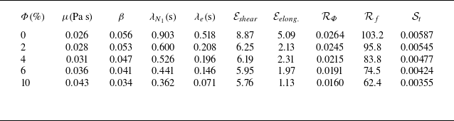
 β=μp/μ=μp/(μs+μp+μΦ)
 RΦ=ργ˙dp2/μ
 Rf=ργ˙δ2/μ
 St=(1/18)(ρΦdp2/μ)
 γ˙=1000s−1

 Φ

 Φ

 γ˙=1000s−1
 α
 τ∞

 τ∞=τ(t→12h)
 Φ
 γ˙
 Φ
 γ˙
 τs+Φ=4πri2hμs+pΩi/1−η2
 Φ
 τ∞/τs+Φ
 γ˙


 α
 Φ
 γ˙

 Φ=0%
 10%

 γ˙c

 Dreal=|τ−τlam|
 γ˙
 Dm
 D~m

 Φ=0,6%
 γ˙=500,1000s−1

 Φ=0−6%
 γ˙=500−1000s−1

 δs
 Φ
 Lm
 δs
 dp

 δs
 Lm
 Φc


 Open access

