

INTRODUCTION
Cold-water coral reefs support large and diverse ecosystems (Fosså et al., Reference Fosså, Mortensen and Furevik2002; Roberts et al., Reference Roberts, Wheeler, Freiwald and Cairns2009; van Oevelen et al., Reference van Oevelen, Duineveld and Lavaleye2009) and typically exist in deep water, between 100 and 3000 m with a few exceptions and with relatively constant cold temperatures, normally between 4 and 12°C. Such reefs face a number of threats to their continued existence, such as ocean acidification (IPCC, 2007), and mechanical destruction due to fishery activities (Fosså et al., Reference Fosså, Mortensen and Furevik2002). The impact of climate change on cold-water reef ecosystems has yet to be quantified but the threat posed by an increase of environmental temperatures beyond the physiological tolerances of reef fauna is very real (IPCC, 2007). The rapid changes of temperature measured at Tisler cold-water coral reef are described here and the wider oceanographic and environmental chain of causation is discussed.
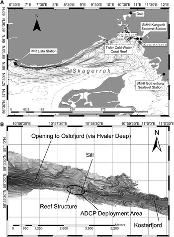
Tiser Reef is located in the north-eastern Skagerrak Strait (Figure 1A). The largest portion of water in the Skagerrak is derived from the North Sea and ingressing water is characterized by strong haline stratification in the upper layers (Gustafsson, Reference Gustafsson1999). Such ingressing surface water into the Skagerrak mixes with brackish water from the Kattegat as it follows the cyclonic flow around the strait. Increased inflow from the Atlantic Ocean to the North Sea results in an increased flow to the Skagerrak being strongly influenced by westerly winds (Winther & Johannessen, Reference Winther and Johannessen2006).
(A) Location of Tisler cold-water coral reef in the north-eastern Skagerrak. Tisler Reef is located on the sill of the Kosterfjord; (B) the Kosterfjord connects to the Norwegian Trench and the Oslofjord via the Hvaler Deep.

The Kattegat, with a mean depth of 26 m, and the Belt Sea, with a mean depth of 13 m, separate the Skagerrak from the brackish Baltic Sea (Stigebrandt, Reference Stigebrandt1983). Bottom water is advected from the Skagerrak into the Kattegat and Baltic while surface water flow is in the opposite direction. The Baltic Sea has a net inflow to the Skagerrak (Winther & Johannessen, Reference Winther and Johannessen2006) with an outflowing (towards the Baltic) mean salinity (psu) 17.4 and an inflowing mean salinity of 8.7 (Stigebrandt, Reference Stigebrandt1983).
The Skagerrak Front, between the Skagerrak and the Kattegat, governs inflow and outflow from the Baltic Sea. The Skagerrak Front is geostrophically balanced and typically exists between Jutland, at the northern tip of Denmark, across to the Swedish coast (Stigebrandt, Reference Stigebrandt1983). The front has a dynamic position and may change rapidly due to the barotrophic forcing of sea height differences and sea surface wind forcing (Rodhe, Reference Rodhe1996).
Freshwater runoff from fjords also plays a large part in the surface salinities in the Skagerrak. A large number of fjords, such as the Gullmar Fjord, Sweden, and the Oslofjord, Norway, empty into the Skagerrak. The topography and hydrography of fjords cause them to be dynamic environments but sheltered from extreme currents, consequently, a large number of Lophelia pertusa reefs are found in fjords on the Norwegian coastline (Freiwald et al., Reference Freiwald, Fosså, Grehan and Koslow2004; Roberts et al., Reference Roberts, Wheeler and Freiwald2006).
Tisler Reef (Figure 1A) is dominated by L. pertusa and is thought to be between 8600 and 8700 years old (Wisshak & Ruggeberg, Reference Wisshak and Ruggeberg2006). The reef is 2 km long, 200 m wide at its widest point and has a depth-range of between 90 and 120 m. Situated on the sill of the Kosterfjord, north of the Tisler Islands, the reef connects the Kosterfjord with the Hvaler Deep, which in turn is connected to the Oslofjord and the Norwegian Trench (Figure 1B). The Kosterfjord is not a fjord in the traditional sense as it is open to the sea at both ends and stretches 48 km along the west coast of Sweden, to the east of the Koster Islands (Dahlgren et al., Reference Dahlgren, Wiklund, Kallstrom, Lundalv, Smith and Glover2006). The environmental conditions at the reef are similar to the larger Skagerrak with strong baroclinic stratification of the water masses and a wide temperature range with February and March the coldest months, often bringing surface ice (Wisshak & Ruggeberg, 2005). The semidiurnal tidal amplitudes of the Skagerrak are very low at 0.05 ms−1 and 0.1 ms−1 for neap and spring tides respectively (Lavaleye et al., Reference Lavaleye, Duineveld, Lundälv, White, Guihen, Kiriakoulakis and Wolff2009), thus residual flows are the dominant driver of current at the reef. Residual and tidal flows over the reef are primarily along the channel axis, which runs from north-west to south-east (Lavaleye et al., Reference Lavaleye, Duineveld, Lundälv, White, Guihen, Kiriakoulakis and Wolff2009; Wagner et al., Reference Wagner, Purser, Thomsen, Jesus and Lundälv2011).
Tisler Reef is composed of large coral stands of over 1 m in height as well as smaller outcrops of coral growth. The living coral is surrounded by an area of coral rubble fragments. The topography of the reef is very rough with coral framework forming banks and depressions of several metres. The surface is a matrix of coral skeleton and rubble, infilled with sediment and organic material as well as benthic organisms, their tubes and shells. Ongoing survey work of the ecosystem and coral framework of Tisler Reef is performed by the Sven Lovén Centre using the high definition cameras on-board a remotely-operated vehicle. The reef exhibits some damage, most likely caused by trawling but for the most part is healthy with a high number of associated infauna (Lavaleye et al., Reference Lavaleye, Duineveld, Lundälv, White, Guihen, Kiriakoulakis and Wolff2009).
One sponge species typical of Tisler Reef is Geodia barretti (Bowerbank, Reference Bowerbank1858). Geodia barretti (also known in the literature as G. baretti) is one of the most commonly encountered large sponge species on the Norwegian coast, growing to a diameter of 1 m, and is distributed widely in large clusters along the margins of the North Atlantic, from northern Norway, to western Sweden to Greenland (Klitgaard & Tendal, Reference Klitgaard and Tendal2004) though the species has also been reported in the Aegean Sea (Voultsiadou & Vafidas, Reference Voultsiadou and Vafidis2004). Areas of seabed covered by G. barretti and related sponges, typically found deeper than 50 m, are referred to in fishermen's charts as Ostur, meaning ‘cheese bottom', due to the sponge's white, round appearance (Klitgaard & Tendal, Reference Klitgaard and Tendal2004) and is a testament to the sponges abundance in these areas. Sponges typically make up 19% of the biomass at cold-water coral sites on the Rockall Bank (van Oevelen et al., Reference van Oevelen, Duineveld and Lavaleye2009), and most likely play a role in the carbon cycling at Tisler Reef.
A primary scientific interest in G. barretti is the extraction of biologically active compounds with pharmacological applications, such as barettin (Lidgren & Bohlin, Reference Lidgren and Bohlin1988). Despite the scientific and commercial interest in G. barretti, little is known of its in situ physiological tolerances. Here we describe the observation of temperature shocks at Tisler Reef, explore the causes of these shocks and discuss the potential relationship between the shocks and the loss of sponge biomass.
MATERIALS AND METHODS
As coral reefs are delicate ecosystems, equipment cannot simply be deployed as free-fall landers. Instead a remotely-operated vehicle (ROV) was used in order to select sites and deploy instruments with precision in order to minimize the impact of sampling at the reef. All instrument deployments were made with the aid of a Sperre SUB-fighter 7500 DC ROV, which is equipped with high definition photographic equipment, a manipulator arm, sample collection tray, conductivity–temperature–depth (CTD) probes and an acoustic transducer for accurate underwater positioning. The use of an ROV allowed for a careful deployment of instruments. Precise geographical positioning information of equipment deployments using the ROV telemetry data allowed for accurate mapping and recovery without surface markers.
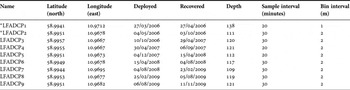
To date more than forty-four months of current flow data have been recorded at Tisler Reef using an RDI 300 kHz Acoustic Doppler Current Profiler (ADCP). Nine deployments of the ADCP, mounted in a gimbal, were made at the reef (Table 1). In all but the first two deployments a Seabird Electronics SBE 37 MicroCAT temperature and conductivity logger was attached to the frame. Data were collected at sample intervals of 20 or 30 minutes and each deployment was made independently. Most of the deployments were made on or near the sill of the Kosterfjord (Figure 1B), which delimits the south-eastern edge of the large reef structure. Exact instrument positioning was typically dictated by sea state conditions and the requirement to not damage coral, therefore the deployments were not made at the same spot on each occasion. The distribution of the low frequency ADCP deployments spanned no more than 500 m at its most extreme and the vertical range of the long-term datasets is between 70 and 100 m above the seabed.
300 kHz Acoustic Doppler Current Profiler deployments made at Tisler Reef. Absence of a MicroCAT TS logger is denoted by*.

The attached Seabird MicroCAT measured the bottom temperature and conductivity of the water. The internal clock of both units was synchronized and for each deployment, a matching sample interval was set. On recovery of the deployment, the ADCP data were quality controlled using beam correlation and acoustic signal strength data.
Wind and sea level data for the Skagerrak were kindly provided by the Swedish Meteorological and Hyrdrographic Institute. The wind data were collected at North Koster Island, which lies 8 km south of Tisler Reef. The Skagerrak sea-level data were collected at the Kungsvik (north) and Gothenburg (south) stations, and span the 150 km of the Swedish Skagerrak coast. Temperature profile data from the Lista station were provided by the Institute for Marine Research, Norway (IMR). The station lies 250 km west of Tisler Reef and is the closest temperature profile station with available data for the period of interest. Despite its distance from the reef and its position on the periphery of the North Sea, the Lista station is hydrodynamically connected to the northern Skagerrak by the Norwegian Coastal Current, which follows the Norwegian coast from the Oslofjord to the Norwegian Sea.
RESULTS
Temperatures
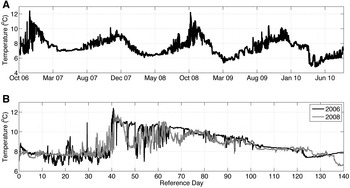
The measurements of temperature at the reef show a typical cycle of seasonal change (Figure 2A). The average weekly temperature was observed to drop from a high of almost 10°C in late November to a low of 6.5°C in early April. The rise in temperatures between April and November was observed to be slow and steady. The standard deviation in mean annual temperatures is small during the spring (<0.5°C) with little variation continuing through the summer months. Towards the end of the year, from October through to December (week 40 onwards), the standard deviation in temperature was seen to increase (>1°C). This increase in the standard deviation is attributable to different patterns of temperature increase in the latter months of the year.
(A) Composite of bottom temperature time-series compiled from T-S loggers deployed at Tisler Reef between September 2006 and September 2010; (B) a comparison of the 2006 (black) and 2008 (grey) temperature events measured near the seabed. The 2006 event occurred three weeks earlier in the year than the 2008 event. A time scale of days since early onset is used for comparison. In both cases the temperatures rose by over 4°C in less than 24 hours.

During the autumn months of the deployment the bottom temperature at the reef was observed to increase rapidly to over 12°C in both 2006 and 2008, while in 2007 and the recorded portion of 2009, the maximum temperatures were less than 11°C.
The temperature event in 2006 commenced on 21 November and the event of 2008 commenced on 30 October. The 2006 event was preceded by a sharp spike in temperature to almost 11°C, 10 days prior to the main temperature event. This feature was not evident in the 2008 event (Figure 2B).
There is a difference of 21 days in the calendar occurrence of the temperature events in 2006 and 2008. The patterns of rapid changes in temperatures are, however, remarkably similar. Both 2006 and 2008 time-series show small and short jumps in temperature of approximately 1°C before increasing at almost the same rate (~4°C/24 hours) and to temperatures within 0.2°C of each other (Figure 2B).
The temperature quickly dropped from its peak by 0.5°C during a number of hours before falling by over 3°C in both cases, though the 2006 event showed a greater variability in temperature. The rapid fluctuations in temperature continued for the next 30 days with a period of between weeks and 3 days, though the amplitude decreased over time. After 50 days of oscillation, the temperature became less variable and was observed to cool progressively.
Currents
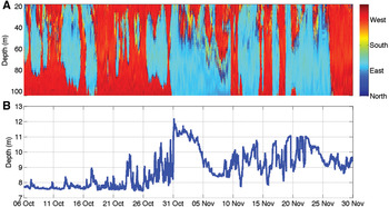
The occurrence of the temperature shock and the oscillations seen within the time-series, correlate strongly with the current direction at the seabed. The temperature jumps in both 2006 and 2008 were preceded by a sustained flow to the north-west (Figure 3A). As the flow reversed, the temperature increased rapidly to its peak before slightly subsiding (Figure 3B). A large initial drop in temperatures in both years was associated with the change in flow for the north-west before jumping again on flow reversal. Successive temperature oscillations were associated with flow reversals; flow to the north-west coinciding with temperature reduction while flow to the south-east correlated with temperature increases.
The 2008 temperature event showing (A) the direction of the water flow through the water column as measured by the low frequency Acoustic Doppler Current Profiler and (B) the bottom temperature measured by the associated T-S logger.

Increases in temperature were associated with the decrease in salinity resulting in decreased σt (density-1000). In 2006 the σt of the water at the seabed varied between 27.4 in the cold phase to as low as 25.5 during the warmest period. The density was observed to swing either side of a σt of between 26.5 and 27 in rapid, episodic events and as the water masses mixed and cooled, the σt variability decreased.
DISCUSSION
In the month preceding both temperature events, the wind, measured at the north Koster station, was above 10 ms−1 30% of the time and was predominantly to the north. The wind occasionally gusted up to gale forces with speeds in excess of 20 ms−1. In both 2006 and 2008, the flow reversal at the seabed, and hence the temperature events, occurred directly after a significant change in the wind characteristics. The 2006 initial temperature spike occurred during a short-lived reversal in wind direction with the major event occurring after a slowing of the wind and deflection to the west (Figure 4A). The 2008 temperature shock was preceded by a reversal in wind direction and a large decrease in speed (Figure 4B).
Progressive vector diagram of the wind measured in the weeks leading up to the (A) 2006 and (B) 2008 temperature shock. Wind was recorded at the nearby Koster Islands by the Swedish Meteorological and Hyrdographical Institute.

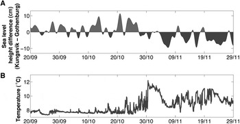
Sea level data collected by the SMHI along the western Swedish coast during both the 2006 and 2008 events shows that the difference between the sea level in the northern and southern Skagerrak increased before the event with a peak difference of 10 cm between Kungsvik in the north and Gothenburg in the south (Figure 5A). The initially relatively high sea level measured at Kungsvik corresponded with the strong winds blowing to the north (Figure 5B) and is a result of the wind piling up the seawater in the northern Skagerrak. The sea level at Kungsvik was then observed to fall quickly while the level at Gothenburg rose immediately after the change in the wind direction.
(A) Sea level difference between Kungsvik in the northern Skagerrak and Gothenburg in the southern Skagerrak during the temperature events of 2008, with a 2 day filter applied to remove tidal influence; (B) 2008 bottom temperature during the same time period.

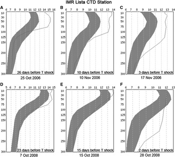
Temperature profile data collected by the IMR at the Lista station were used to estimate the thermocline depth of the northern Skagerrak before and after the temperature shock events of 2006 and 2008. A deepening of the thermocline could potentially allow warmer, summer solar heated surface water to mix with the cooler water below. The temperature shock event of 2006, which occurred on 21 November, was preceded by a deepening of the thermocline from 75 m on 25 October to 125 m on 17 November (Figure 6A–C). The temperatures recorded above the thermocline during this period were also between 1 and 2°C higher than the computed climatology, based on observations from 1942 to 1994. The deepening of the thermocline also corresponded with a weakening in the temperature gradient. These developments in the thermocline were echoed in 2008 though the surface temperatures were as far outside the computed normal values as in 2006 (Figure 6D–F).
Temperature profile data from the IMR Lista station preceding the (A, B & C) 2006 and 2008 (D, E & F) temperature shock events. The dark band displays the computed expected values based on records from 1942 to 1994. Data reproduced courtesy of the Institute of Marine Research, Norway (http://data.nodc.no/stasjone).

Temperature records at Tisler Reef reflect a typical seasonal heating pattern. Differences in the cycle between successive years were evident, with a prominent heating pattern observed during autumn of both 2006 and 2008. The maximum temperatures of 12.5°C recorded during these years are much higher than the maximum temperature of 9°C previously observed at the reef by the nearby Sven Löven Centre for Marine Science (T. Lundälv, personal communication) and occurred rapidly, rising in both cases by 4°C in less than 24 hours. The peak temperatures were not sustained beyond several days. The temperature event of 2006 occurred 21 days later in the year than the 2008 event though the peak temperatures and pattern of occurrence, particularly at onset, are almost indistinguishable.
The warming with a south-east flow indicates that the warm bottom water came via the Oslofjord while the cooler north-west flow came from the Kosterfjord. Temperature changes were observed to occur hours after flow reversals. The shifting of the post-shock temperature time-series between two states, i.e. approximately 10.5 and 8.5°C, suggests the baroclinic movement of a temperature gradient back and forth over the reef.
The temperature shock event of 2006 resulted in a rapid decrease of 1.7 in σt, indicating that the ingress of warmer water was not caused by a density driven flow. The large temperature range at low salinity (between 33.75 and 34) suggests that the gradual increase in density was the result of cooling. A similar T-S pattern was observed in the 2008 event. The significant decrease in salinity, associated with the σt drop, suggests the influence of a freshwater source of warm water. The similarity in the pattern of the events further is suggestive of a common mechanism in the transport of high temperature water to the reef. Such a mechanism would exist on a scale much greater than the reef, thus the array of instrument deployments at Tisler Reef alone is not sufficient for assessing the origin of the warmer temperatures or the driving force behind its delivery.
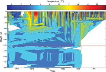
There are no frequent measurements of temperatures at the Tisler Reef that span through several decades. A fish stock survey has, however, been conducted in the Kosterfjord by the Swedish Fisheries Board (personal communications to T. Lundälv) since the 1960s. As part of the survey, CTD measurements were undertaken and, while not complete, give a record of temperatures in the Kosterfjord from 1968 to 2000. Measurements made by the Swedish Fisheries Board within 15 km of Tisler Reef show that temperatures above 9°C were not recorded in the northern Kosterfjord during the sampling (Figure 7). The dataset resolution is variable with time and depth. Surveys became more frequent after 1980 but the depth of sampling was restricted to the upper 40 m.
Conductivity–temperature–depth data from the north of Kosterfjord, close to Tisler Reef, from 1968 to 2000. Data courtesy of the Swedish Meteorological and Hydrographical Institute.

Despite the sampling inconsistencies and the aliasing of the data when presenting such a fragmented time-series, the intention is to show from these data an absence of higher temperature records at depth rather than provide an analysis of trends. It is clear that at no time were temperatures above 9°C recorded below 100 m. Temperatures of over 12°C were only recorded at depths shallower than 70 m, 50 m above the seabed while the 2006 and 2008 temperature shocks were recorded at the seabed. During the 1970s the frequency of sampling was reduced with the result that the individual seasonal cycles could not be identified. Furthermore, in 1991, the sampling of water between 40 m and the seabed was halted resulting in a large gap in temperature time-series at the reef level.
The absence of any temperatures as high as those observed during deployments at Tisler Reef is sufficient to support the claim that the temperature shocks of 2006 and 2008 are, at least, highly unusual events. It is notable that in the late 1980s and early 1990s, water temperatures of between 10 and 12°C were recorded at progressively deeper depths. This may be a result of the increased inflow from the North Atlantic into the North Sea and the elevated sea surface temperatures recorded during this time (Reid et al., Reference Reid, de Fatima Borges and Svendsen2001).
The coincidence of the south and south-westerly winds with the north-westward flow over the reef suggests that the driving force of the warm water transport from the south was the wind. The fall in the salinity during the temperature shocks and the transport of the warm water from the south suggests that the water mass may have come from the Kattegat, through which the low salinity Baltic outflow water enters the Skagerrak. The strong winds blowing north across the Kattegat may therefore have caused a pulse of warm surface water, originating in the Baltic, to escape the Skagerrak front and travel north along the Swedish coast.
The less consistent wind regime before the temperature shock in 2006 may account for the greater short-term variability seen in the bottom temperature measurements during this period. The rapid onset of the current reversal after the wind shifts indicates that flow reversal at the seabed was not directly caused by wind stress. Furthermore, the decrease in density associated with the temperature shocks rules out a current reversal caused by a density driven flow as density was observed to decrease during the shock.
The mechanism for the transport of warm water to Tisler Reef is hypothesized to be a result of above average sea surface temperatures in the Skagerrak and Baltic in conjunction with strong south-easterly winds blowing across southern Scandinavia. The sea level therefore, having piled up in the north, began to equilibrate once the opposing force of the wind was removed. The shift in the position of the high water from north to south occurred just prior to the peak of the temperature shocks and was consistent with the timing of the flow reversal. The equilibrating sea level caused a rapid current flow reversal as water pushed to the south thus carrying the warm, surface-mixed water from the northern Skagerrak back over the reef. Small, unsustained increases in temperature that grew larger before the onset of the temperature shocks were coincident with short, low amplitude shifts of high sea level to the south (Figure 5). This early onset feature of the temperature shock suggests that each sea level change brought the warm front closer to the reef before finally pushing it all the way. A similar pattern was observed in the wake of both temperature shocks where high sea level in the north was associated with sharp drops in the temperature as the warm pulse retreated from the reef. The seeming regularity of the temperature changes after the temperature events is evidence of the migration of the warm front back and forth over the reef. This is borne out by the apparent oscillation of the sea level high position between north and south (Figure 5A) as the Skagerrak sea surface equilibrated after the winds changed.
It is startling that the two known recorded incidents of sudden temperature shock occurred within 23 months of each other and during a period of apparent warming of the mean sea surface temperatures in the region (Reid et al., Reference Reid, de Fatima Borges and Svendsen2001). Such a finding begs the question of a climate change mediated impact on the reef ecosystem. The positive assertion of such a correlation is beyond the scope of this research though these observations are sufficiently alarming as to warrant further, long-term monitoring of environmental parameters at the reef.
The frequency of the events and the correlation with far field environmental parameters will help to test the hypothesis of high temperature water transport to the reef. Regular CTD transects or thermister chain deployment in the Oslofjord and the Kosterfjord will greatly enhance the understanding of the mixing of the water masses involved in the events. The current description of the thermocline dynamics prior to the temperature shock is based on measurements made 250 km from the reef, which while not unreasonable due to the Norwegian Coastal Current linkage, is less than ideal. Similar work in the southern Skagerrak and Kattegat will establish the source of the warm water and determine if a pulse crosses the Skagerrak Front.
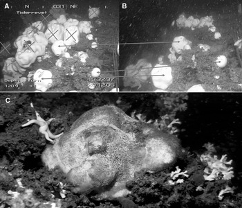
The temperature shock events of both 2006 and 2008 preceded by several weeks the observation, by ROV operators using high definition video cameras at the Sven Löven Centre, of mass mortality in the sponge species Geodia barretti (Bowerbank, Reference Bowerbank1858) at the reef (Figure 8). The mass mortality amongst the sponges (Hogg et al., Reference Hogg, Tendal, Conway, Pomponi, van Soest, Gutt, Krautter and Roberts2010) was anecdotally estimated by observers at 95% in the worst affected areas of the reef, though a more rigorous survey of the mortality has not yet been conducted. The coincidence of the temperature shock events with mass mortality in the species suggests an exceedance of the sponge's physiological limits though the direct cause of the mortality is not known. Though an analysis of the pathway to mortality in sponges is outside the scope of the current research, it is suggested that microbially induced anaerobic degradation may be the cause. Stress has been shown to weaken the immune response of G. baretti, causing a loss of control over intrinsic and foreign bacteria (Hoffmann et al., 2006). The necrosis of G. baretti described by Hoffmann et al. (Reference Hoffmann, Rapp and Reitner2006) resulted in the precipitation of iron sulphide, giving the sponge tissue a black colour.
(A) The presence of the sponge Geodia barretti at a site on Tisler Reef in December 2005. Arrows highlight the missing sponges in (B) November 2008; (C) the sponge tissue turns blue and black as it decays.

Geodia barretti is a very slow growing species (Klitgaard & Tendal, 2006) and though the time required to grow to full diameter is not known, it is estimated to be between several decades and a century (Hogg et al., Reference Hogg, Tendal, Conway, Pomponi, van Soest, Gutt, Krautter and Roberts2010). Any previous mortality event on this scale would necessarily have occurred with a period greater than the maturing time of the sponge. That the vast majority of the standing crop at the reef was apparently removed by rapid temperature increases offers additional support for the rarity of the temperature events.
The increase in temperature to over 12°C on both occasions, which is above some estimates of L. pertusa temperature tolerance (Dodds et al., Reference Dodds, Roberts, Taylor and Marubini2007), means that future temperature events at the reef, if of the same magnitude, may have severe consequences for the health of the reef ecosystem. It should be noted that while mortality of G. baretti was observed at Tisler Reef, no such observations were made of mortality in other phyla. This may be due to specific tolerances to short term, high temperature exposure.
The phenomenon of temperature shock at Tisler Reef has been observed only twice thus the relevant satellite derived sea surface temperature (SST) dataset is currently very limited and is at best suggestive of the source of the warm water pulses. Long term investigation of the heating patterns in the Skagerrak and correlation with future temperature shocks, should they occur, is required to establish a causal relationship between the events at the reef and the wider climate context. One such climate context is the North Atlantic Oscillation teleconnection index (NAO). Increased flow from the north-east Atlantic into the Skagerrak via the North Sea is highly likely to be positively correlated with the NAO (Winther & Johannessen, Reference Winther and Johannessen2006). The NAO values also correlate well with North Sea winter surface temperatures, suggesting that surface heat loss is reduced due to the westerly winds carrying warm, moist air. This correlation is not found during other seasons (van Aken, Reference van Aken2010).
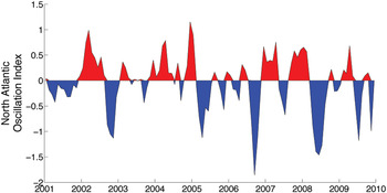
While two data points currently exist for temperature shock occurrence, it is significant that on both occasions the shocks were preceded by at least three months of sustained low NAO values, with a 3 month running mean below −1 (Figure 9), both falling below −1.25 at some point. These strongly low NAO features are very rare in the whole time-series, which dates in some forms back to 1865, and occurring only six times since 1950. Low NAO characterizes an atmospheric pressure condition that would tend to block westerly winds across northern Europe (Hurrell, Reference Hurrell1995). Such a condition would direct south-easterly winds across Scandinavia. Coupled with SST trends and atmospheric data, further analysis and long term monitoring in the Skagerrak may confirm the role of climate in ecosystem change at Tisler Reef.
Three month running mean of North Atlantic Oscillation for the years 2001–2009. Data courtesy of the National Oceanic and Atmospheric Administration, United States of America (http://www.cpc.noaa.gov/products/precip/CWlink/pna/nao_index.html).

ACKNOWLEDGEMENTS
This work was funded by FP6 EU-project HERMES (EC contract no. GOCE-CT-2005-511234). The authors thank the staff of the Sven Lovén Centre for Marine Sciences, Tjärnö. Thanks to the Swedish Meteorological and Hydrographical Institute, the Swedish Fisheries Board and the Institute for Marine Research, Norway for providing data referenced in the text. The authors are grateful for the advice and comments of the three referees who helped to improve the manuscript.