





Nomenclature
-
 $C_{D*},C_{L*}$
-
drag and lift coefficients
-
$C_{\{l*,m*,n*\}}$
-
body-axis moment coefficients
-
$C_{T*},C_{Q*}$
-
propeller thrust and torque coefficients
-
$C_{\{X,Y,Z\}}$
-
body-axis force coefficients
-
$D$
-
drag force [N]
-
$\mathcal{D}$
-
propeller diameter [m]
-
${\bf I}$
-
aircraft inertia tensor [kg m
${^2}$
] -
$I_p$
-
propeller moment of inertia [kg m
${^2}$
] -
$I_{\{x,y,z,xz\}}$
-
aircraft moments and product of inertia [kg m
${^2}$
] -
$J$
-
advance ratio [-]
-
${\bf J}$
-
Fisher information matrix
-
$L$
-
lift force [N]
-
$\mathcal{N}(\boldsymbol{\mu },\Sigma )$
-
multivariate Gaussian distribution
-
${\bf P}$
-
parameter covariance matrix
-
$P_{*}$
-
power [W]
-
$Q$
-
propeller torque [Nm]
-
$\boldsymbol{R}$
-
SO(3) rotation matrix
-
$S$
-
wing planform area [
${\mathrm m^2}$
] -
$T$
-
propeller thrust [N]
-
$V_a$
-
true airspeed [m/s]
-
$X_u$
-
speed-damping [N s m
${^{-1}}$
] -
$Z_u$
-
heave-damping [N s m
${^{-1}}$
] -
$a_x,a_y,a_z$
-
specific force in body axes [
${\mathrm m/s^2}$
] -
$b$
-
wingspan [m]
-
$\bar {c}$
-
mean aerodynamic chord [m]
-
$g$
-
gravitational acceleration [
${\mathrm m/s^2}$
] -
$h$
-
altitude [m]
-
$k_{\alpha }$
-
blending steepness parameter [
${\mathrm{rad}^{-1}}$
] -
$m$
-
aircraft mass [kg]
-
$m_r$
-
ice-rod mass [kg]
-
$p,q,r$
-
body-axis angular rates [rad/s]
-
$p^{\ast },q^{\ast },r^{\ast }$
-
nondimensional rates [-]
-
$\dot p,\dot q,\dot r$
-
body-axis angular accelerations [
${\mathrm{rad}/{\textrm s}^2}$
] -
$\bar {q}$
-
dynamic pressure [Pa]
-
$\boldsymbol{q}$
-
attitude quaternion
-
$\boldsymbol{r}$
-
position vector [m]
-
$u,v,w$
-
body-axis linear velocities [m/s]
-
${\mathrm w}_{\alpha }$
-
angle-of-attack blending weight [-]
-
$\boldsymbol{v}$
-
linear velocity vector [m/s]
-
$\boldsymbol{w}$
-
wind velocity vector [m/s]
-
$x,y,z$
-
body-axis position coordinates [m]
-
$\Delta _{\alpha }$
-
blending interval width [rad]
-
$\Omega _p$
-
propeller angular speed [rad/s]
-
$\alpha _{0}$
-
blending centre [rad]
-
$\alpha$
-
angle-of-attack [rad]
-
$\beta$
-
angle of sideslip [rad]
-
$\delta _{{\mathrm a}},\delta _{\mathrm {e}}$
-
aileron and elevator deflections [rad]
-
$\delta _{el},\delta _{er}$
-
left and right elevon deflections [rad]
-
$\delta _t$
-
normalised throttle [-]
-
$\zeta _{ph}$
-
phugoid damping ratio [-]
-
$\eta _*$
-
efficiency or scale factor [-]
-
$\boldsymbol{\theta }$
-
model parameter vector
-
$\mu$
-
mean value
-
$\rho$
-
air density [
${\mathrm{kg/m}^3}$
] -
$\sigma$
-
standard deviation
-
$\phi ,\theta ,\psi$
-
Euler roll, pitch, yaw angles [rad]
-
$\boldsymbol{\omega }$
-
angular rate vector [rad/s]
-
$\omega _{ph}$
-
phugoid natural frequency [rad/s]
-
$ {}_a$
-
aerodynamic subscript
-
$ {}_w$
-
wind subscript
-
$ {}^{\star }$
-
trimmed state superscript
-
$(\! \cdot \!)^{+},(\! \cdot \!)^{-}$
-
high- and low-
$\alpha$
regimes in blended model -
$ \{{\mathrm b}\}$
-
body frame
-
$ \{{\mathrm n}\}$
-
north-east-down frame


1.0 Introduction
The operational envelope of small fixed-wing unmanned aerial vehicles (UAVs) is rapidly expanding to include high-intensity commercial logistics and year-round, beyond visual line-of-sight (BVLOS) missions [1]. As these missions scale, extended exposure to environmental hazards, such as atmospheric in-flight icing, has emerged as a limiting factor [2]. While typical battery-powered multirotor flights are often restricted to 15–30 minutes, fixed-wing platforms can easily fly for hours [Reference Tacconi, Marini, Saraceno, Foresti, Cinque and Mecca3]. This extended flight capability elevates atmospheric icing to a severe operational hazard. Several recent climatological assessments aimed at quantifying this threat indicate that low-altitude UAVs can encounter icing conditions at non-negligible rates, especially during winter months [Reference Sørensen, Borup, Hann, Bernstein and Pellicano4, Reference Hansbø and Hoelsæter5].
Although the hazard of atmospheric icing has been extensively studied and mitigated in general aviation, these traditional frameworks cannot be directly applied to smaller, unmanned platforms. Aerodynamically, small UAVs operate at significantly lower Reynolds numbers and employ much thinner aerofoil sections than conventional aircraft, making them inherently more sensitive to the performance penalties of ice accretion and surface contamination [Reference Hann and Johansen6, Reference Cao, Tan and Wu7]. Beyond these aerodynamic differences, the direct transfer of conventional physical ice protection systems (IPSs) to small fixed-wing UAVs remains constrained by stringent size, weight and power (SWaP) limitations [Reference Hann and Johansen6, Reference Jones and Gross8]. While these constraints do not preclude icing mitigation altogether, they typically restrict IPS usage, such as allowable duty cycles or spatial coverage. Consequently, small UAVs (less than 25 kg) can benefit greatly from information-driven strategies that adapt guidance, navigation and control (GNC) and IPS behaviour based on the aircraft’s aerodynamic state, rather than relying on predefined anti-icing and de-icing cycles. Successfully implementing such strategies requires the flight controller to recognise ice accretion in flight, making an ice detection system (IDS) a critical prerequisite. Although the latest literature reviews highlight the availability of various IDS technologies [Reference Løw-Hansen, Hann, Stovner and Johansen9, Reference Maio, Moore, Cook and Potluri10], their direct integration into small UAVs remains challenging. Consequently, since existing commercial sensors are often prohibitively expensive or exceed allowable SWaP budgets, there is still a need for alternative detection methodologies tailored specifically for lightweight aircraft.
Accurate aerodynamic modelling of icing effects can therefore be used as a tool to enable safe and robust UAV operations in icing conditions. Model-based detection, decision support and adaptive control strategies all presuppose the availability of reliable rigid-body models that capture how ice accretion alters aerodynamic forces, moments and dynamic modes. For manned aircraft, this need has long been recognised. Previous work has shown that icing effects can be incorporated into flight dynamics models through structured parameter extensions [Reference Bragg, Hutchison and Merret11], later refined into regime-dependent
 $\Delta$
-model frameworks with explicit stall and separation representations [Reference Deiler12, Reference Deiler13]. These modelling concepts, supported by extensive icing wind tunnel (IWT) and flight-test campaigns, have enabled detailed analysis of icing-induced changes in stability and control characteristics for general aviation aircraft [Reference Broeren, Potapczuk, Lee, Woodard, Bragg and Smith14–Reference Cao, Wu and Su16].
While these foundational methodologies provide a vital reference, their specific aerodynamic results cannot be directly transferred to smaller unmanned platforms. In contrast to large transport aircraft, (lighter) business jets or regional aircraft, small UAVs possess unique airframe configurations (e.g. position and design of wing(s) and empennage) and fundamentally different baseline mass properties. Specifically, the relationship between vehicle size and accreted ice mass is disproportionate for smaller UAVs, leading to unique dynamic penalties. Therefore, although the system identification techniques developed for manned aviation offer an excellent methodological baseline, the dynamic response of iced UAVs remains an open research question that must be evaluated using dedicated flight-test data.
To date, experimentally identified icing models for small fixed-wing UAVs remain largely absent from the open literature. A recent review of flight-test-based system identification studies for small UAVs [Reference Løw-Hansen, Hann, Gryte, Johansen and Deiler17, Table 2] shows that while numerous clean-aircraft models exist, such as those developed for model-based navigation [Reference Longobardi and Skaloud18], none explicitly address atmospheric icing. Existing UAV icing research has instead focused primarily on static aerodynamic degradation and ice morphology [Reference Hann, Hearst, Sætran and Bracchi19–Reference Han22], or on propulsion system effects such as propeller icing [Reference Liu, Li, Chen, Tian and Hu23–Reference Løw-Hansen, Müller, Coates and Johansen28]. Although these studies consistently demonstrate substantial performance penalties, they do not quantify how icing alters the flight dynamic modes and control characteristics for small fixed-wing UAVs.
Several authors have proposed model-based icing detection and adaptive control strategies as surveyed in Refs [Reference Løw-Hansen, Hann, Stovner and Johansen9, Reference Maio, Moore, Cook and Potluri10], and recent large-scale efforts such as work done within the Horizon 2020 project SENS4ICE [Reference Deiler29] further highlight the importance of model-based decision support. However, these approaches fundamentally rely on the availability of accurate rigid-body aerodynamic models for iced configurations. For small fixed-wing UAVs, such models have yet to be established experimentally, so recent research on flight control in icing conditions [Reference Adelina Ghindaoanu, Gryte, Reinhardt and Johansen30–Reference Kleiven, Gryte and Johansen32] has relied on models with limited validation.
Motivated by this gap, the present work addresses the following research questions (RQs):
-
RQ1: How does wing icing alter the aerodynamics of a small fixed-wing UAV?
-
RQ2: Can quasi-steady models capture these icing-induced changes?
-
RQ3: What are the implications for IPS/IDS and GNC of small fixed-wing UAVs?
To answer these questions, we perform a flight-test-based system identification study of the Skywalker X8 UAV (Figure 1 and Table 1) in clean and wing-iced configurations. Artificial ice shapes are produced in an IWT (Section 2) and installed on the airframe; the resulting rigid-body changes are quantified and accounted for in the analysis (Section 3). Using a structured quasi-steady aerodynamic model (Section4) and output-error identification on dedicated manoeuvres (Section 5), we quantify icing-induced aerodynamic changes and assess model adequacy and identification challenges. Results and implications are presented in Sections 6–8.
Physical properties of the flight-ready Skywalker X8 UAV

Table 1. Long description
A table listing the physical properties of the Skywalker X8 UAV. The table has two columns: Property and Value. It contains eight rows with the following data: Row 1: Property, Mass; Value, 3.730 kilograms. Row 2: Property, Moment of inertia; Value, Ix, 0.335 kilograms per meter squared. Row 3: Property, Moment of inertia; Value, Iy, 0.140 kilograms per meter squared. Row 4: Property, Moment of inertia; Value, Iz, 0.400 kilograms per meter squared. Row 5: Property, Product of inertia; Value, Ixz, -0.029 kilograms per meter squared. Row 6: Property, Mean chord length; Value, 0.36 meters. Row 7: Property, Wing span; Value, 2.10 meters. Row 8: Property, Planform area; Value, 0.75 square meters. Row 9: Property, Sweep angle; Value, 28.3 degrees.
Skywalker X8 UAV takeoff during the flight campaign near Trondheim, Norway.

2.0 Creation of the artificial ice shapes
2.1 Icing wind tunnel campaign
The artificial ice shapes used for the comparative clean/iced flight tests were generated during an IWT campaign at the VTT Technical Research Centre of Finland in Helsinki [Reference Tiihonen, Jokela and Makkonen33]. The facility is an open-loop tunnel with a 700 mm x 700 mm test section. The 3D wing segment was mounted in an open-jet configuration at the test section exit using external brackets (see Figure 2). The wing was fixed at an angle-of-attack of
 ${4}^\circ$
, selected as a representative cruise condition derived from prior flight-test campaigns with this UAV family [Reference Løw-Hansen, Hann, Gryte, Johansen and Deiler17, Reference Borup, Fossen and Johansen34]. Previous characterisations of the facility’s flow field revealed substantial spatial variability in the liquid water content (LWC) outside the tunnel core [Reference Hann, Müller and Lindner35]. However, the calibration also identified a 200 mm
 $\times$
100 mm central region exhibiting low LWC variation. To ensure uniform droplet exposure and minimise localised trajectory distortions near the mounting brackets, the representative test segment was limited to a width of 150 mm (as can be recognised by the chord-wise markings on the wing in Figure 2).
Placement of the wing in the IWT during accretion experiments. The visible chord-wise lines mark the boundaries of three splittable wing sections, with the central 150 mm portion serving as the isolated test segment for representative ice extraction. (The tape covering the splits was changed between experiments).

In defining the meteorological conditions for this uniform test region, the continuous maximum icing conditions detailed in FAA Part 25, Appendix C [Reference Jeck36] were used as a guiding framework. While these conditions provide a widely recognised baseline for manned aviation, their representativeness for the lower-altitude regimes of small UAVs remains an open research question [Reference Hann and Johansen6]. Specifically, the IWT target conditions were set to an LWC of
 $0.52\,{\mathrm {g/m}^3}$
with a median volume diameter (MVD) of
 $27.4\,{\unicode{x03BC}{\mathrm m}}$
at
 $-10\,^{\circ }\textrm {C}$
. Although this LWC is higher than the nominal Appendix C continuous maximum envelope for this droplet size (
 ${0.26}\,{\mathrm {g/m}^3}$
), a more substantial ice accretion was deliberately targeted. This over-scaling ensures that the resulting geometry is representative of intentionally pronounced rime ice accretions. Consequently, the ice generates an aerodynamic penalty of sufficient magnitude to clearly overcome flight-test measurement noise and state-estimation uncertainties, such as the
 $\sigma _\alpha = 0.6^\circ$
angle-of-attack variance detailed in subsection 5.4, allowing the clean and iced states to be robustly distinguished in the final identified models.
The tunnel airspeed was maintained at 25 m/s, slightly above the UAV’s nominal cruise speed of 18 m/s, to ensure consistency with a concurrent experimental baseline. Furthermore, to simulate realistic prolonged exposure to an icing environment during BVLOS operations, the accretion duration was set to 20 min. At this selected airspeed, a 20-minute duration yields a theoretical cloud traverse distance close to the standard 17.4 NM (32.2 km) horizontal extent defined for Appendix C continuous maximum encounters (21.5 min at 25 m/s).
2.2 Photogrammetry digitisation and 3D printing
After the ice accretion run, the middle segment was detached and trimmed to retain a 118 mm spanwise ice extent. To capture its complex geometry, the ice shape was digitised into a full 3D model using the photogrammetry methodology detailed in Ref. [Reference Hann, Müller and Lindner35]. By comparing the physical weight of the sample to the volume of the 3D model, the density of the accreted ice was computed to
 ${0.4}\,\,{\mathrm {g/cm}^3}$
, which falls within the realistic range of
 ${0.1}$
to
 ${0.9}\,{\mathrm {g/cm}^3}$
reported in Ref. [Reference Macklin37]. A comparison between the original ice, the digitised model and the resulting print is shown in Figure 3.
The final flight-test ice shapes were produced by additive manufacturing (3D printing). Since only a 118 mm spanwise segment was available, the digitised ice was linearly scaled according to the chord length variation along the entire wing span, with six segments per wing. Right-wing segments were obtained by mirroring about the chordwise axis. While this linear scaling assumption provides a baseline for system identification experiments, true spanwise ice accretion on swept wings is more complex. As demonstrated in large-scale swept-wing icing studies [Reference Camello, Lee, Lum and Bragg38, Reference Potapczuk and Broeren39], the ice shape depends on the variations in wing geometry, such as changes in the leading-edge radius.
Comparison of the original ice shape created in the IWT and the digitised photogrammetry ice shape.

Figure 3. Long description
Panel A: A photograph of the original rime ice shape. The ice shape is irregular and rough, with varying textures and protrusions. Panel B: A photogrammetry model of the ice shape. The model closely resembles the original ice shape, capturing its irregularities and textures. Panel C: A 3D printed shape of the ice. The printed shape is green and has a rough, textured surface similar to the original ice shape. Panel D: A line graph showing ice shape 2D cross sections. The x-axis is labeled ‘x (m)’ and the y-axis is labeled ‘y (m)’. The graph includes three lines: a black line labeled ‘Clean’, a blue line labeled ‘IWT maximum combined cross section’, and a black line labeled ‘IWT 75 mm cross section’. The lines show different profiles of the ice shape cross sections.
Furthermore, testing swept-wing segments in confined wind tunnel environments can alter the spanwise stagnation and attachment line locations. This effect has been shown to be significant for large commercial transport wings and requires explicit computational matching procedures to correct the flow over truncated models [Reference Fujiwara and Bragg40]. For the work presented here, where the goal is a representative ice shape for system identification, these corrections are deemed less critical given the other limitations of the ice shape generation method – notably the deliberately over-scaled LWC and the linear spanwise scaling of a single 118 mm segment.
The mass of the segments was matched to the total estimated ice mass by adjusting infill settings during 3D printing. Table 2 summarises the estimated segment masses from the fitted 3D model and the corresponding printed masses; small segment-level deviations are expected due to chord scaling, print tolerances and discrete infill settings, while the total mass match is preserved. Printing was performed using an Ultimaker S5 3D-printer. The installed ice shapes are shown in Figure 4. The total added mass was 420 g (210 g per wing), resulting in a 6 mm forward shift of the centre of gravity (CG) measured by a 3-point balance and weight meter.
Estimated and 3D-printed ice-segment masses (rounded to the nearest gram)

Table 2. Long description
A table comparing estimated and 3D-printed ice-segment masses across six segments. The table has 7 rows and 8 columns. Column headers are Seg. 1, Seg. 2, Seg. 3, Seg. 4, Seg. 5, Seg. 6, and Total. Row labels are Estimated and 3D printed. Row 1: Estimated, Seg. 1, 62 g; Seg. 2, 62 g; Seg. 3, 34 g; Seg. 4, 24 g; Seg. 5, 18 g; Seg. 6, 13 g; Total, 213 g. Row 2: 3D printed, Seg. 1, 58 g; Seg. 2, 48 g; Seg. 3, 34 g; Seg. 4, 28 g; Seg. 5, 24 g; Seg. 6, 18 g; Total, 210 g.
Ice shapes used for the iced configuration flights, installed continuously from root to tip. The complete leading-edge accretion on each wing consists of six 3D-printed segments: one black at the root, three coloured in the middle and two black near the tip.

As seen in Figure 4, the installed ice shapes introduce a sharp geometric edge at the inboard root, which is expected to generate localised flow separation and artificially contribute to the identified drag penalty. Conversely, this artificial representation does not cover secondary airframe components that would accrue ice in practice, omitting realistic drag contributions. To perfectly isolate the aerodynamic effects of leading-edge accretion, future experimental iterations should incorporate spanwise edge smoothing and/or full-airframe icing models.
3.0 Rigid-body changes due to wing icing
Leading-edge icing affects the identified flight dynamics not only through aerodynamic degradation, but also through rigid-body changes. The added ice mass is distributed away from the fuselage centreline, increasing the moments of inertia and shifting the CG forward. To capture these effects, the accretion is approximated by six cylindrical rods per wing, attached symmetrically along the span as illustrated in Figure 5. Each rod contribution is shifted to the aircraft CG using the parallel-axis theorem
 \begin{align} I_{{\mathrm UAV}} = I_{{\mathrm rod}} + m_r d^2, \end{align}
where
 $m_r$
is the rod mass and
 $d$
is the perpendicular distance from the rod centroid to the axis of rotation.
Relative placement of the ice-rod segments used for modelling rigid-body changes.

The total mass increased from 3.73 to 4.15 kg, corresponding to an increase of 11%. The ice shapes are installed symmetrically about the aircraft
 $x$
–
 $z$
plane (left–right symmetry), such that the added mass does not influence
 $I_{xy}$
and
 $I_{yz}$
. The vertical offset of the added ice relative to the
 $x$
–
 $y$
plane is assumed negligible, implying a negligible contribution to
 $I_{xz}$
; consequently, the products of inertia are assumed unchanged. The resulting inertia tensors are given by
 \begin{align} \mathbf{I}_{\text{clean}} &= \begin{bmatrix} 0.335 &\quad 0 &\quad -0.029 \\[1pt] 0 &\quad 0.140 &\quad 0 \\[1pt] -0.029 &\quad 0 &\quad 0.400 \end{bmatrix} \;\text{kg m}^2 , \ \mathbf{I}_{\text{iced}} &= \begin{bmatrix} 0.480 &\quad 0 &\quad -0.029 \\[1pt] 0 &\quad 0.145 \quad& 0 \\[1pt] -0.029 &\quad 0 &\quad 0.550 \end{bmatrix} \;\text{kg m}^2 \end{align}
While a higher-fidelity volumetric integration of the exact 3D ice shape or experimental validation via swing testing could yield more precise mass properties, the expected gain is minimal relative to the added uncertainty. Because the added ice mass is concentrated at the leading edge, its contribution to the aircraft’s total inertia is heavily dominated by its distance from the CG (
 $m_r d^2$
), rather than its local geometric details. Consequently, the difference between an exact 3D volume integration and the rod-segment approximation is negligible for the overall rigid-body dynamics. Furthermore, conducting physical swing tests (e.g. via a bifilar pendulum) on fixed-wing UAVs introduces non-negligible aerodynamic added-mass effects due to entrained air, which inherently complicates the measurements [Reference Jardin and Mueller41]. Correctly isolating these effects would require considerable effort, which in this case is left for future work.
The CG location was measured using a dedicated CG balance rig, with all quantities referenced to a centre of origin (CO) coincident with the inertial measurement unit (IMU)/estimator frame. The measured longitudinal offsets are
 \begin{align*} {\bf r}_{{\mathrm {CO}}\rightarrow {\mathrm {CG}}}^{{\mathrm {clean}}} = [0.110\,\,0\,\,0]^\top \,{\mathrm m}, \qquad {\bf r}_{{\mathrm {CO}}\rightarrow {\mathrm {CG}}}^{{\mathrm {iced}}} = [0.116\,\,0\,\,0]^\top \,{\mathrm m}, \end{align*}
corresponding to a forward shift of 6 mm. The CG was not measured along the vertical axis; the vertical offset is assumed unchanged and treated as a source of uncertainty.
Aerodynamic forces and moments are evaluated about the CG. The aerodynamic centre (AC) is assumed to coincide with the CG in both configurations. This simplifying assumption is reasonable because the CG is not expected to change during flight, and the distance between the true AC and the CG is small. From classical static stability theory [Reference Anderson42, Chap. 4.9], the offset is proportional to the static margin:
 \begin{align} x_{{\mathrm {ac}}} - x_{{\mathrm {cg}}} = - \bar {c} \frac {C_{m\alpha }}{C_{L\alpha }} \end{align}
Based on the identified coefficients in subsection 6.4, this yields a theoretical offset of 2.7 cm in the clean case (with the AC located behind the CG).
Finally, the accreted ice modifies the effective reference geometry by changing the aerofoil geometry and increasing the chord length. Based on the reconstructed ice geometry, the mean aerodynamic chord increases from
 $\bar {c}= {0.36}$
to
 $\bar {c}_{{\mathrm{ ice}}}={0.38}\,{\mathrm m}$
, and the projected wing planform area increases from
 $S= {0.75}$
to
 $S_{{\mathrm {ice}}}\approx {0.81}\,{\mathrm m^2}$
. These iced-geometry values are reported for completeness; however, to ensure direct comparability between clean and iced results, all aerodynamic coefficients in this paper are nondimensionalised using the clean reference quantities
 $(S,\bar {c},b)$
for both configurations.
4.0 Aerodynamic modeling
This section outlines the methodology for aerodynamic system identification. It details the procedures required to isolate bare-airframe aerodynamics from propulsive effects, reconstruct aerodynamic forces and moments from flight kinematics, and formulate a model structure capable of characterising both the clean and iced configurations.
4.1 Computed coefficients from flight data
System identification is performed by fitting parametric coefficient models to equivalent aerodynamic coefficients reconstructed from flight data. The reconstruction follows Ref. [Reference Løw-Hansen, Hann, Gryte, Johansen and Deiler17] and uses IMU-specific force measurements expressed in the body frame and transformed to the CG
 $(a_x,a_y,a_z)$
, together with gyroscope body rates
 $(p,q,r)$
. The IMU measurements are corrected using the bias estimates from the ArduPilot’s extended Kalman filter (EKF) before any transformations are applied. Angular accelerations
 $(\dot p,\dot q,\dot r)$
are obtained from
 $(p,q,r)$
using a 5-point local quadratic least-squares differentiator [Reference Morelli and Klein43]. The measurements are scaled by dynamic pressure
 $\bar {q}=\frac {1}{2}\rho V_a^2$
, where
 $V_a$
is the true airspeed at CG and
 $\rho$
is the air density. Using these quantities (with thrust and torque compensation from subsection 4.2), the reconstructed coefficients are computed as:
 \begin{align} C_X {} &=\frac {m a_x-T}{\bar {q} S}, \\[-9pt] \nonumber \end{align}
 \begin{align} C_Y {} &=\frac {m a_y}{\bar {q} S},\\[-9pt] \nonumber \end{align}
 \begin{align} C_Z {} &=\frac {m a_z}{\bar {q} S}, \\[-9pt] \nonumber \end{align}
 \begin{align} C_l {} &=\frac {1}{\bar {q} S b}\left [I_x \dot {p}-I_{x z}(p q+\dot {r})+\left (I_z-I_y\right ) q r + Q\right ],\\[-9pt] \nonumber \end{align}
 \begin{align} C_m {}& =\frac {1}{\bar {q} S \bar {c}}\left [I_y \dot {q}+\left (I_x-I_z\right ) p r+I_{x z}\left (p^2-r^2\right ) + I_p \Omega _p r\right ],\\[-9pt] \nonumber \end{align}
 \begin{align} C_n {} &=\frac {1}{\bar {q} S b}\left [I_z \dot {r}-I_{x z}(\dot {p}-q r)+\left (I_y-I_x\right ) p q - I_p \Omega _p q\right ]. \\[9pt] \nonumber \end{align}
The propeller gyroscopic coupling terms
 $I_p\Omega _p r$
and
 $-I_p\Omega _p q$
, where
 $I_p$
is the propeller inertia and
 $\Omega _p$
is the propeller speed, are retained in Equations (4e) and (4f), whereas the inertial torque term proportional to the propeller angular acceleration
 $I_p\dot {\Omega }_p$
is omitted. In normal flight, this can often be justified since the motor speed is fairly constant. Moreover, the motor-speed measurement is available at only 10 Hz, and numerical differentiation introduces uncertainty that outweighs the benefit of including this term. Nevertheless, in settings where
 $\Omega _p$
is not measured and is instead inferred from electrical power and efficiency models, including
 $I_p\dot {\Omega }_p$
may be beneficial; this was considered in Ref. [Reference Løw-Hansen, Hann, Gryte, Johansen and Deiler17].
4.2 Propulsion and actuator models
The propulsion model provides the thrust and torque compensation necessary to separate airframe drag from thrust-induced acceleration. The torque and thrust coefficients,
 $C_Q$
and
 $C_T$
, are represented as second-order polynomials of the nondimensional advance ratio
 $J$
:
 \begin{align} J {}&= \frac {2 \pi V_a}{ \Omega _p \mathcal{D}} ,\\[-9pt] \nonumber \end{align}
 \begin{align} C_Q(J) {}&= C_{Q0} + C_{Q1} J + C_{Q2} J^2 \;, \\[-9pt] \nonumber \end{align}
 \begin{align} C_T(J) {}&= C_{T0} + C_{T1} J + C_{T2} J^2 \;, \\[10pt] \nonumber \end{align}
where
 $\mathcal{D}$
is the propeller diameter,
 $V_a$
is the airspeed and
 $\Omega _p$
is the propeller angular speed.
To account for configuration-dependent installation effects, the dimensional torque and thrust are computed with empirical scaling factors,
 $\eta _Q$
and
 $\eta _T$
:
 \begin{align} Q {}= \eta _Q \frac {\rho \mathcal{D}^5}{4 \pi ^2} C_Q(J) \Omega _p^2 \;, \\[-9pt] \nonumber \end{align}
 \begin{align} T {}= \eta _T \frac {\rho \mathcal{D}^4}{4 \pi ^2} C_T(J) \Omega _p^2 \;. \\[10pt] \nonumber \end{align}
The Skywalker X8 UAV used in this study was flown with an Aero-naut CAM Z Carbon 14x8 folding propeller. The baseline polynomial parameters, in Tables 3 and 4, were identified from isolated wind-tunnel experiments following the methodology in Ref. [Reference Løw-Hansen, Müller, Coates and Johansen28].
Thrust and torque coefficients

Table 3. Long description
A table comparing thrust and torque coefficients. The table has two columns labeled C_T and C_Q, each containing three rows of data. Under C_T, the values are: C_T0, 0.1537; C_T1, -0.1059; C_T2, -0.0967. Under C_Q, the values are: C_Q0, 0.0084; C_Q1, 0.0100; C_Q2, -0.0200.
Propeller parameters

Table 4. Long description
The table lists various propeller parameters and their corresponding values. It includes the diameter, moment of inertia, thrust scale, and torque scale. The diameter is given as 0.3556 meters or 14 inches. The moment of inertia is 3.46 times 10 to the power of -4 kilograms square meters. The thrust scale is 1.00 for clean and 0.81 for iced conditions. The torque scale is 1.00 for clean and 0.83 for iced conditions.
For the clean UAV configuration, it is assumed that the installed pusher propeller behaves sufficiently similarly to the isolated wind-tunnel tests. Therefore, the baseline models are used without scaling (
 $\eta _T = 1.0$
,
 $\eta _Q = 1.0$
). However, applying these uninstalled models directly to the iced configuration introduces significant physical inconsistencies. The iced airframe forces the powertrain into a regime where the polynomials identified in the wind tunnel over-predict the propulsive output. To quantify this discrepancy, two apparent operational efficiencies are defined based on the unscaled wind-tunnel models: the apparent electromechanical efficiency
 $\eta _{\mathrm{mech} }$
and the apparent overall propulsive efficiency
 $\eta _{\mathrm {prop}}$
:
 \begin{align} \eta _{\mathrm{mech} } = \frac {Q \, \Omega _{p}}{P_{{\mathrm {batt}}}} \quad , \quad \eta _{\mathrm {prop}} = \frac {T \, V_{a}}{P_{{\mathrm {batt}}}} \;, \end{align}
where
 $P_{{\mathrm {batt}}}$
is the power drawn from the battery, computed as the product of the measured voltage and current. Evaluating the mean of these ratios over the respective flights yields:
-
• Clean configuration:
$\eta _{\mathrm{mech} } \approx 0.8959$
,
$\eta _{\mathrm {prop}} \approx 0.6454$
. -
• Iced configuration:
$\eta _{\mathrm{mech} } \approx 1.0809$
,
$\eta _{\mathrm {prop}} \approx 0.7962$
.


The unphysical iced apparent electromechanical efficiency (
 $\eta _{\mathrm{mech} } = 1.0809$
) proves that the uninstalled propeller model over-predicts loads when extrapolated to the iced UAV configuration. This notable loss of propulsive performance could be linked to the pusher propeller ingesting the turbulent wake generated by the sharp inboard edges of the artificial ice shapes, motivating the use of smoothed spanwise transitions for future experiments. Aerodynamically, because the propeller operates in this momentum deficit, using the true airspeed (
 $V_a$
) to compute the advance ratio (
 $J$
) neglects the locally reduced inflow velocity, mathematically inflating the predicted torque and thrust. Lacking an in-flight thrust meter to decouple these aero-propulsive effects, the uncorrected output error (OE) algorithm would erroneously absorb this inflated thrust and torque into overestimated aerodynamic drag and rolling moments. Indeed, initial estimations using unscaled models yielded a power penalty equal to 230% of the measured change.
To prevent this, the iced powertrain model is anchored to the clean apparent efficiency baseline using scaling factors
 $\eta _T = 0.8106$
and
 $\eta _Q = 0.8289$
. Although true propeller efficiency likely degrades further in the turbulent iced wake, making additional corrections without direct thrust measurements would be arbitrary. Thus, this baseline anchoring is a deliberate engineering choice: it neutralises the propulsive over-prediction and forces any true propulsive degradation to be absorbed by the identified aerodynamic coefficients. As will be demonstrated in subsection 6.6, this strategy yields a representative systemic model that reasonably bounds the modelled power penalty due to ice accretion.
Model parameters for a
 ${2}^{{\mathrm{nd}}}$
order servo system controlling the elevons

Table 5. Long description
A table displaying model parameters for a servo system controlling the elevons. The table has four columns and one row. The columns are labeled Natural frequency, Damping, Input delay, and Deflection range. The row contains the following values: Natural frequency is 100 rad/s, Damping is 0.707, Input delay is 0.12 s, and Deflection range is ±19°.
The servo delay was determined from clean experiment data by computing the mean lag between the initial elevator step inputs and the resulting pitch-rate response, while the natural frequency and damping were carried over from Ref. [Reference Løw-Hansen, Hann, Gryte, Johansen and Deiler17]. The resulting servo model parameters are listed in Table 5.
4.3 Aerodynamic coefficient model
The coefficient parametrisation determines which aerodynamic states are required for model evaluation and simulation. A classical representation in angle-of-attack
 $\alpha$
, angle of sideslip
 $\beta$
, nondimensional angular rates and elevator/aileron inputs is adopted to align with the aircraft icing literature, where changes in lift and drag are commonly reported as functions of angle-of-attack and ice accretion [Reference Bragg, Hutchison and Merret11–Reference Deiler13, Reference Hann, Hearst, Sætran and Bracchi19, Reference Lindner, Wallisch and Hann21, Reference Deiler, Ohme, Raab, Mendonca and Silva44–Reference Bragg, Broeren and Blumenthal46].
The aerodynamic angles are computed starting from the body-axis velocity and the estimated wind, in component form:
 \begin{align} \begin{bmatrix} u_a \\ v_a \\ w_a \end{bmatrix} = \begin{bmatrix} u - u_w \\ v - v_w \\ w - w_w \end{bmatrix} ,\end{align}
with true airspeed
 $V_a$
and aerodynamic angles computed as:
 \begin{align} V_a = \sqrt {u_a^2 + v_a^2 + w_a^2}, \quad \alpha = \tan ^{-1}\!\left (\frac {w_a}{u_a}\right ), \quad \beta = \sin ^{-1}\!\left (\frac {v_a}{V_a}\right ). \end{align}
The nondimensional angular rates are given by:
 \begin{align*} p^{\ast } = \frac {p b}{2 V_a}, \quad q^{\ast } = \frac {q \bar {c}}{2 V_a}, \quad r^{\ast } = \frac {r b}{2 V_a}. \end{align*}
The Skywalker X8 is a flying-wing UAV with right and left elevons
 $(\delta _{er},\delta _{el})$
, which are mapped to equivalent elevator and aileron deflections
 $(\delta _{\mathrm {e}},\delta _{{\mathrm a}})$
by:
 \begin{align} \begin{bmatrix} \delta_{\textit{e}} \\ \delta_{\textit{a}} \end{bmatrix} = \frac{1}{2} \begin{bmatrix} 1 &\quad 1 \\ -1 &\quad 1 \end{bmatrix} \begin{bmatrix} \delta_{\textit{er}} \\ \delta_{\textit{el}} \end{bmatrix} \end{align}
The model terms were selected using a stepwise regression algorithm applied to a candidate pool of linear, non-linear and coupled aerodynamic regressors. Initial modelling attempts with a globally smooth, quasi-steady longitudinal formulation produced convergent fits, but closer inspection of reconstructed coefficient trends (see Section 6) showed that a global linear model could not simultaneously fit the distinct lift, pitching-moment and drag curves at positive and negative angles of attack, suggesting a regime change near
 $\alpha \approx {0}^{\circ }$
. This is consistent with the break-point modelling approach for iced aircraft presented in Ref. [Reference Deiler12].
Accordingly, the longitudinal model is represented by two regimes blended by a continuous weight
 ${\mathrm w}_\alpha$
, defined as:
 \begin{align} {\mathrm w}_{\alpha } = \frac {1}{1 + \exp \!((\alpha -\alpha _0) k_{\alpha })}, \qquad k_{\alpha } = \frac {2\log (9)}{\Delta _{\alpha }} \end{align}
where the factor
 $2\log\! (9)$
is chosen so that the weight transitions from 0.9 to 0.1 over the interval
 $\Delta _\alpha$
centered at
 $\alpha _0$
. In this case, the interval was set to
 $\Delta _\alpha = {0.0175}\,\mathrm {rad}={1}^{\circ }$
.
During the initial system identification, the centre of this transition (
 $\alpha _0$
) was treated as a free parameter and converged within a band around
 ${-2}^{\circ }$
and
 ${0}^{\circ }$
for both configurations. However, allowing the break-point to wander within this range degraded the overall convergence and stability of the aerodynamic derivatives. To prevent this,
 $\alpha _0$
was fixed at the data-driven consensus value of
 ${-0.02}\,\mathrm {rad}$
(approximately
 $-1.1^{\circ }$
).
The two resulting regime models are denoted by superscripts
 $^+$
and
 $^-$
and are blended by
 ${\mathrm w}_\alpha$
. Candidate break-point extensions were selected by inspection of coefficient trends and refined through trial-and-error to avoid numerical ill-conditioning. To keep the structure minimal, only coefficients required by the data were split between regimes; in particular, the lift and pitching-moment terms were split only for the iced configuration.
The resulting longitudinal model is:
 \begin{align} C_L^+ {}&= C_{L0} + C_{L\alpha } \alpha + C_{Lq} q^{\ast } + C_{L\delta \mathrm {e}} \delta _{\mathrm {e}}\;, \\[-9pt] \nonumber \end{align}
 \begin{align} C_L^- {}&= C_{L0} + C_{L\alpha }^- \alpha + C_{Lq} q^{\ast } + C_{L\delta \mathrm {e}}^- \delta _{\mathrm {e}}\;, \\[-9pt] \nonumber \end{align}
 \begin{align} C_D^+ {}&= C_{D0} + C_{Dq} q^{\ast } + C_{Dk1} C_L^+ + C_{Dk2} {C_L^+}^2\;, \\[-9pt] \nonumber \end{align}
 \begin{align} C_D^- {}&= C_{D0} + C_{Dq}^- q^{\ast } + C_{Dk1}^- C_L^- + C_{Dk2}^- {C_L^-}^2\;, \\[-9pt] \nonumber \end{align}
 \begin{align} C_m^+ {}&= C_{m0} + C_{m\alpha } \alpha + C_{mq} q^{\ast } + C_{m\delta \mathrm {e}} \delta _{\mathrm {e}}\;, \\[-9pt] \nonumber \end{align}
 \begin{align} C_m^- {}&= C_{m0} + C_{m\alpha }^- \alpha + C_{mq} q^{\ast } + C_{m\delta \mathrm {e}}^- \delta _{\mathrm {e}}\;, \\[-9pt] \nonumber \end{align}
 \begin{align} C_L {}&= (1-{\mathrm w}_{\alpha }) C_L^+ + {\mathrm w}_{\alpha } C_L^-\;, \\[-9pt] \nonumber \end{align}
 \begin{align} C_D {}&= (1-{\mathrm w}_{\alpha }) C_D^+ + {\mathrm w}_{\alpha } C_D^-\;, \\[-9pt] \nonumber \end{align}
 \begin{align} C_m {}&= (1-{\mathrm w}_{\alpha }) C_m^+ + {\mathrm w}_{\alpha } C_m^-\;. \\[9pt] \nonumber \end{align}
The lateral model is kept symmetric:
 \begin{align} C_Y {}&= C_{Y0} + C_{Y\beta } \beta + C_{Yp} p^{\ast } + C_{Yr} r^{\ast } + C_{Y\delta {\mathrm a}} \delta _{{\mathrm a}}\;, \\[-9pt] \nonumber \end{align}
 \begin{align} C_l {}&= C_{l0} + C_{l\beta } \beta + C_{lp} p^{\ast } + C_{lr} r^{\ast } + C_{l\delta {\mathrm a}} \delta _{{\mathrm a}}\;, \\[-9pt] \nonumber \end{align}
 \begin{align} C_n {}&= C_{n0} + C_{n\beta } \beta + C_{np} p^{\ast } + C_{nr} r^{\ast } + C_{n\delta {\mathrm a}} \delta _{{\mathrm a}}\;. \\[9pt] \nonumber \end{align}
A thrust-related term was also tested in the drag model in Equations (15c) and (15d) similar to Ref. [Reference Løw-Hansen, Hann, Gryte, Johansen and Deiler17], but did not yield a meaningful improvement. In this case, it led to an unrealistically small zero-lift drag
 $C_{D0}$
, implying significant drag reductions at low throttle. Thrust-related terms were therefore excluded from the final drag model.
5.0 Experiment setup
This section summarises the flight-test campaign and the data processing steps used to obtain measurements for the system identification process.
Overview of performed system identification manoeuvres at 18 m/s

Table 6. Long description
A table comparing different system identification maneuvers at 18 m/s. The table has six rows and six columns. Column headers are Direction, Type, Pulse duration, Amplitude, Fitting, and Validation clean/iced. Row 1: Direction, Lateral; Type, 1-2-1; Pulse duration, [0.1 s, 0.5 s]; Amplitude, [15°, 8°]; Fitting, [3,3]; Validation clean/iced, [3,3]/[3,3]. Row 2: Direction, Lateral; Type, Doublet; Pulse duration, [0.1 s, 0.6 s, 3.0 s]; Amplitude, [15°, 8°, 5°]; Fitting, [3,"3",3]; Validation clean/iced, [3,"4",2]/[3,"3",2]. Row 3: Direction, Longitudinal; Type, 3-2-1-1; Pulse duration, [0.2 s, 1.5 s]; Amplitude, [12°, 6°]; Fitting, [3,3]; Validation clean/iced, [3,3]/[2,2]. Row 4: Direction, Longitudinal; Type, Doublet; Pulse duration, [0.3 s, 2.3 s]; Amplitude, [12°, 6°]; Fitting, [3,3]; Validation clean/iced, [2,3]/[5,3].", "EDH": "
5.1 Flight campaign
Three flight tests were performed within a three-hour window on the morning of 19th November 2024 at Brenslan, Trondheim, Norway. Cruise altitude and airspeed were held at approximately 100 m and 18 m/s. The ground temperature was
 $-2\,^{\circ }\textrm {C}$
, with estimated wind speeds of 2 m/s to 4 m/s. Each flight was powered by a 16 V, 8 Ah battery. Because the iced configuration increased power consumption, the iced dataset was split across two flights:
-
• Flight 1: Clean configuration (lateral and longitudinal manoeuvres).
-
• Flight 2: Iced configuration (lateral manoeuvres).
-
• Flight 3: Iced configuration (longitudinal manoeuvres).
In total, 106 manoeuvres were extracted: 53 in the clean configuration and 53 in the iced configuration. Each manoeuvre lasted 15–35 s yielding approximately 2200 s of experiment data. Roughly half of this dataset captures active dynamic excitations, while the remainder establishes the steady-state trim conditions before and after each manoeuvre.
5.2 Excitation manoeuvres and closed-loop execution
A set of pre-programmed excitation signals was injected by an onboard companion computer (Khadas Vim3) to achieve repeatable excitation while maintaining safe flight. A detuned custom attitude controller [Reference Coates, Reinhardt, Gryte and Johansen47] ran on the companion computer in parallel with ArduPilot, utilising ArduPilot’s guidance-driven roll and pitch references alongside the EKF-based attitude estimate. During the flight, a separate script on the companion computer injected the excitation signal offsets; consequently, the realised control surface deflections were superimposed on the closed-loop response rather than acting as clean open-loop perturbations.
The manoeuvre set follows standard flight system identification practice and consists of four manoeuvre families (lateral 1-2-1, lateral doublet, longitudinal 3-2-1-1 and longitudinal doublet). Within these families, pulse durations and amplitudes were varied, giving nine distinct excitations in total; the full set is summarised in Table 6. The pulse parameters were selected based on the clean-aircraft campaign in Ref. [Reference Løw-Hansen, Hann, Gryte, Johansen and Deiler17]. Moreover, prior to flight testing, ground experiments were conducted to map pulse-width modulation (PWM) commands to elevon deflection angles, ensuring that the desired deflection angles are correctly translated from degrees to the commanded PWM.
For each configuration, 27 manoeuvres were used for parameter estimation and the remaining 26 manoeuvres were reserved for validation presented in Section 6.
Summary of primary data sources. All data were resampled to the reference EKF time series at 20 Hz

Table 7. Long description
A table with 8 rows and 3 columns. The columns are labeled Data type, Source, and Logged frequency. The rows are as follows: Row 1: Data type, Attitude, linear velocity; Source, Estimated (ArduPilot EKF); Logged frequency, 20 Hz (reference). Row 2: Data type, Acceleration and rate biases; Source, Estimated (ArduPilot EKF); Logged frequency, 20 Hz. Row 3: Data type, Horizontal wind state; Source, Estimated (ArduPilot EKF); Logged frequency, 20 Hz. Row 4: Data type, Acceleration, angular rate; Source, Measured (ICM20602/ICM20948); Logged frequency, 50 Hz. Row 5: Data type, GNSS; Source, Measured (Here3+); Logged frequency, 5 Hz. Row 6: Data type, Airspeed (pitot-static); Source, Measured (MS4525DO); Logged frequency, 10 Hz. Row 7: Data type, Motor speed; Source, Measured (HW-BQ2017); Logged frequency, 10 Hz. Row 8: Data type, Battery voltage and current; Source, Measured (Analog Power Module); Logged frequency, 10 Hz. Row 9: Data type, Control commands; Source, Generated (Khadas Vim3); Logged frequency, 25 Hz.
Although the experiments were executed with stabilising feedback, the identification uses the measured plant data in the sense of `direct’ closed-loop identification, i.e. applying a prediction error method directly to input–output data while ignoring possible feedback. In the prediction-error framework, this approach remains consistent provided that the tracked reference sufficiently excites the relevant dynamics and the model structure is adequate [Reference Ljung48, Chap. 13.4]. A detailed closed-loop perspective is given by Forssell and Ljung [Reference Forssell and Ljung49], and a recent flight-test application of closed-loop identification, albeit using a frequency-domain joint input–output approach, is discussed in Ref. [Reference Ågren, Ruan, Malpica, Withrow-Maser and Meyn50].
5.3 Flight data processing and synchronisation
The Skywalker X8 flight stack is built around the Cube Orange autopilot running ArduPilot firmware. Logged signals include EKF-estimated attitude and velocity, EKF-estimated horizontal wind, inertial measurements from the IMU, global navigation satellite system (GNSS) position and velocity, pitot-static airspeed, motor speed, battery voltage and current and the injected control commands from the companion computer. A reference time base was established from the EKF velocity timestamps, yielding a sampling frequency of 20 Hz. All channels were resampled to this reference time base using linear interpolation. Table 7 summarises the primary data sources and their original sampling rates.
5.4 Estimator and sensor measurement limitations
While the EKF does not explicitly estimate vertical wind, several factors suggest that the resulting reconstructed aerodynamic angles remain suitable for comparative analysis. The experiments were conducted within a three-hour window on a day with light winds; as shown in Figure 6, the average horizontal wind magnitude varied by only 1 m/s between flights. Given that the vertical wind component in the atmospheric boundary layer is typically several orders of magnitude smaller than the horizontal component [Reference Stull51, Chap. 1.2], changes in the mean vertical bias between flights are expected to be negligible. As an order-of-magnitude check, a vertical wind shift of 0.1 m/s at
 $V_a \approx {18}\,{\mathrm {m/s}}$
would correspond to
 $\Delta \alpha \approx {0.3}^\circ$
.
Averaged EKF state variances during system identification manoeuvres

Table 8. Long description
A table comparing state variances in clean and iced conditions. The table has 3 columns and 8 rows. The columns are labeled ‘State’, ‘Clean variance’, ‘Iced variance’, and ‘Unit’. The rows are labeled with different states and their corresponding variances. Row 1: State v_n, Clean variance 2.013 10^-2, Iced variance 2.111 10^-2, Unit (m/s). Row 2: State v_e, Clean variance 2.020 10^-2, Iced variance 2.113 10^-2, Unit (m/s). Row 3: State v_d, Clean variance 1.241 10^-2, Iced variance 1.227 10^-2, Unit (m/s). Row 4: State w_n, Clean variance 1.243 10^-2, Iced variance 1.226 10^-2, Unit (m/s). Row 5: State w_e, Clean variance 1.078 10^-2, Iced variance 1.082 10^-2, Unit (m/s). Row 6: State q0, Clean variance 4.642 10^-5, Iced variance 4.930 10^-5, Unit -. Row 7: State q1, Clean variance 7.603 10^-6, Iced variance 7.760 10^-6, Unit -. Row 8: State q2, Clean variance 7.611 10^-6, Iced variance 7.736 10^-6, Unit -. Row 9: State q3, Clean variance 3.175 10^-5, Iced variance 3.296 10^-5, Unit -.
Angle-of-attack
 $\alpha$
and sideslip
 $\beta$
are not measured directly but are reconstructed from the EKF states, making them subject to estimation uncertainty. The computation involves the body velocities, wind velocities and attitude quaternion
 $[\boldsymbol{v}^{{\mathrm n}}, \boldsymbol{w}^{{\mathrm n}}, \boldsymbol{q}]$
, which are first transformed to the body frame in CG and then used as shown in Equations (11) and (12). To quantify the output uncertainty, a Monte Carlo analysis was performed. Specifically, to determine the uncertainty in the angle-of-attack at the nominal trim condition,
 $N = 50000$
samples were drawn from a multivariate Gaussian distribution given by:
 \begin{align} \boldsymbol{x} \sim \mathcal{N}\left (\boldsymbol{\mu }_{trim}, \Sigma _{EKF}\right ) \end{align}
where
 $\boldsymbol{x} = [\boldsymbol{v}^{{\mathrm n}}, \boldsymbol{w}^{{\mathrm n}}, \boldsymbol{q}]^T$
and
 $\boldsymbol{\mu }_{trim}$
represents the identified trimmed states for steady level flight at
 $V_a = 18\,{\mathrm {m/s}}$
and zero wind. The diagonal covariance matrix
 $\Sigma _{EKF}$
is populated by the mean EKF variances in Table 8 available from the recorded experiments. As the vertical wind component is not estimated by the ArduPilot EKF, its variance was approximated as the average of the estimated horizontal wind variances,
 $\sigma ^2_{\boldsymbol{w}d} = \frac {1}{2}(\sigma ^2_{\boldsymbol{w}n} + \sigma ^2_{\boldsymbol{w}e})$
.
Horizontal wind magnitude and direction estimated by the ArduPilot EKF during the experiments.

Figure 6. Long description
Panel A: A histogram displays the probability density of wind magnitude in meters per second (m/s) for clean and iced conditions. The x-axis represents wind magnitude ranging from 1.5 to 3.5 m/s, and the y-axis represents probability density. The clean condition data is shown in orange, while the iced condition data is shown in blue. The histogram shows that the wind magnitude for clean conditions peaks around 2.2 m/s, while for iced conditions, it peaks around 3.2 m/s. Panel B: A polar plot shows wind direction in degrees with the x-axis representing wind direction from 0 to 360 degrees and the y-axis representing the magnitude of the wind. The clean condition data is represented by a red arrow pointing towards 180 degrees, and the iced condition data is represented by a blue arrow pointing towards 270 degrees.
Propagating these samples through the kinematic transformations and evaluating Equation (12) yields an aggregated standard deviation of
 $\sigma _\alpha \approx {0.6}^\circ$
. While a systematic bias in the angle-of-attack primarily affects the constant intercept terms (e.g.
 $C_{L0}$
,
 $C_{m0}$
), identified slope coefficients are less susceptible as they are constrained by the dynamic excitation during manoeuvres. Crucially, as the identical state-estimation and identification pipeline is applied to both configurations, the relative trends (deltas) between clean and iced parameters remain reliable, even if absolute magnitudes are subject to the baseline estimation uncertainty.
5.4.1 Pitot-static probe limitations
Although pitot-static measurements provide an independent airspeed source, simple pitot tubes are subject to well-known errors during highly dynamic manoeuvres, particularly at high-flow angles and under unsteady conditions [Reference Larson52]. Specifically, rapid pitch variations can introduce nonphysical high-frequency oscillations into the measured airspeed as shown in Figure 7.
Because airspeed defines the dynamic pressure used to nondimensionalise all aerodynamic coefficients, propagating these sensor-induced oscillations would artificially contaminate the identified models. While transforming the measured airspeed to the CG, through the lever arm
 ${\bf r}_{{\mathrm pitot}\rightarrow {\mathrm CO}} = $
 $[\!-0.504\,\,0\,\,0.096]^\top \,{\mathrm m}$
(
 ${\mathrm {CO}}_z \approx {\mathrm {CG}}_z$
), accounts for the kinematic lever arm, it does not eliminate the observed aerodynamic artefacts. To mitigate this, the true airspeed used for dynamic pressure computation is instead derived from the EKF kinematic state estimates transformed to CG (
 $V_{a,\mathrm {EKF}}$
). As shown in Figure 7, this estimator-derived airspeed accurately tracks the low-frequency trend while remaining insensitive to the high-frequency artefacts correlated with the pitch rate.
Aerodynamic parameters and weighted outputs used during estimation

Table 9. Long description
A table with 27 maneuvers and their corresponding aerodynamic parameters and weighted outputs. The table is divided into two main sections: longitudinal and lateral maneuvers. Each section lists specific parameters and their weighted outputs. The table has 10 rows and 4 columns. The columns are labeled as follows: Data, Parameter, Weighted outputs, Parameter, Weighted outputs. The rows are grouped into different types of maneuvers: 6 longitudinal 3-2-1-1, 6 longitudinal doublet, 6 lateral 1-2-1, and 9 lateral doublet. Each row lists the specific parameters and their weighted outputs for each maneuver type. The parameters and weighted outputs are listed in pairs for each maneuver type.
Note: The listed outputs constitute the full set available; depending on manoeuvre and convergence behaviour, some output weights were disabled during fitting iterations.
5.5 Weighted outputs and parameter groups
The aerodynamic parameters were estimated using a weighted output set comprising kinematic states, angular rates, accelerations and reconstructed force/moment coefficients. To reduce reliance on estimated states, body-axis velocities were not directly used as weighted outputs. Table 9 summarises the parameter groups and weighted outputs.
Measured and estimated airspeed comparison.

As demonstrated in Ref. [Reference Løw-Hansen, Hann, Gryte, Johansen and Deiler17], classic OE formulations [Reference Jategaonkar53] that weight only time-domain kinematic outputs can struggle to converge for small fixed-wing UAVs when direct flow angle measurements (e.g. from a five-hole probe) are unavailable, and estimated flow angles are used instead. Unlike large aircraft, which benefit from high inertial stability and high-fidelity direct air-data measurements, small UAVs are highly susceptible to wind gusts and must frequently rely on noisy, estimator-reconstructed states. This degrades the kinematic signal-to-noise ratio. To overcome these limitations, we employ a hybrid OE method that additionally weights the reconstructed aerodynamic coefficients during parameter fitting. Because these pseudo-measurements are derived from the same state and air-data sensors, their inclusion violates the maximum-likelihood assumption of uncorrelated measurement noise. Nevertheless, this augmented formulation provides essential force and moment constraints, improving numerical conditioning and ensuring a physically consistent model.
The parameter estimation is performed using a Gauss–Newton output-error method. In each iteration, the parameter update
 $\Delta \boldsymbol{\theta }$
is obtained by solving
 \begin{align} \Delta \boldsymbol{\theta } = {\bf J}^{-1}\,{\bf g}, \end{align}
where
 ${\bf g}$
denotes the gradient of the negative log-likelihood cost function, and
 ${\bf J}$
is a Gauss–Newton approximation of the associated Hessian,
 \begin{align} {\bf J} = \sum _{k=0}^{N-1} \left ( \frac {\partial {\bf y}(k)}{\partial \boldsymbol{\theta }} \right )^{\!T} {\bf R}^{-1} \left ( \frac {\partial {\bf y}(k)}{\partial \boldsymbol{\theta }} \right ) \end{align}
where
 ${\bf y}(k)$
denotes the model output vector and
 ${\bf R}$
the measurement noise covariance matrix.
In the maximum-likelihood formulation implemented in DLR’s FITLAB toolbox for MATLAB [Reference Deiler, Mönnich, Seher-Weiß and Wartmann54],
 ${\bf J}$
represents an estimate of the Fisher information matrix [Reference Jategaonkar53, Chap. 4.XVII]. The parameter covariance is estimated as
 ${\bf P}={\bf J}^{-1}$
and reported uncertainties correspond to standard deviation estimates
 $\sigma (\theta _i)=\sqrt {P_{ii}}$
. The uncertainty estimates assume independent and identically distributed (IID) residuals; in closed-loop identification residuals are often correlated, so the reported values reflect the precision around a local optimum and may underestimate the true uncertainty, particularly in the presence of model mismatch and unmodeled dynamics. Since Gauss–Newton is a local method, the solution is highly sensitive to initialisation and can easily fall into nonphysical local optima; to mitigate this, parameters in this study were initialised using a combination of equation-error estimates and previously identified models [Reference Løw-Hansen, Hann, Gryte, Johansen and Deiler17].
6.0 Results
The results section first quantifies the measured differences between the clean and iced datasets using reconstructed aerodynamic coefficients, and then assesses how well the identified models reproduce these trends, including the implied changes in stability and damping.
6.1 Observed aerodynamic changes in the flight data
A comparative overview of the aerodynamic coefficients reconstructed from the clean and iced experiments according to Equation (4) is shown in Figure 8. The excitation manoeuvres drive the UAV through rapid, high-amplitude attitude changes spanning both positive and negative angles of attack, which enables a direct clean–iced comparison over a broader longitudinal envelope than is typically available in manned-aircraft icing datasets.
Comparison of the aerodynamic coefficients reconstructed from the clean and iced configuration experiments. The shown data includes both the training and validation sets.

Figure 8. Long description
The image contains six scatter plots comparing aerodynamic coefficients for clean and iced configurations of small UAVs. Each plot uses blue dots for clean configurations and orange dots for iced configurations. Panel A: A scatter plot of the lift coefficient (C L) versus angle of attack (α in degrees). The data points show a positive correlation for both clean and iced configurations, with iced configurations generally having lower lift coefficients. Panel B: A scatter plot of the moment coefficient (C m) versus angle of attack (α in degrees). The data points are more scattered, but a slight positive correlation is visible for both configurations. Panel C: A scatter plot of the lift coefficient (C L) versus drag coefficient (C D). The data points show a negative correlation, with iced configurations generally having higher drag coefficients. Panel D: A scatter plot of the side force coefficient (C Y) versus sideslip angle (β in degrees). The data points show a roughly linear relationship, with iced configurations having slightly different slopes. Panel E: A scatter plot of the inboard rolling moment coefficient (C l) versus sideslip angle (β in degrees). The data points are scattered around zero, with no clear trend for either configuration. Panel F: A scatter plot of the normal force coefficient (C n) versus sideslip angle (β in degrees). The data points show a positive correlation, with iced configurations generally having higher normal force coefficients.
The reconstructed longitudinal coefficients exhibit several distinct features. Notably, the iced configuration shows a clear increase in drag, especially at higher angles of attack. Furthermore, the lift and drag profiles display an asymmetry around
 $\alpha \approx 0^\circ$
that suggests an aerodynamic regime change, while the iced pitching-moment exhibits a noticeably flatter slope at small angles of attack. In contrast, no corresponding asymmetry is evident in the lateral coefficients, consistent with the lateral model being kept symmetric.
6.2 Static lift–drag characteristics and break-point behaviour
To visualise the identified longitudinal behaviour without measurement noise and manoeuvre transients, Figure 9 shows the static lift curve, lift–drag curve and lift-to-drag ratio for the clean and iced models evaluated without any control surface deflection (
 $\delta _{\mathrm {e}}= 0^\circ$
) and pitch rate (
 $q= 0\,{\mathrm {rad/s}}$
). The break-point formulation yields two smoothly blended regimes. As demonstrated in the lift coefficient plot, the lift generation is only slightly degraded by the ice accretion, showing a minor reduction in lift slope primarily at positive angles of attack. Instead, the most dominant aerodynamic penalty is the increase in drag. The iced lift–drag curve is shifted to higher
 $C_D$
values across most of the flight envelope. This substantial drag increase at positive angles of attack significantly degrades the aircraft’s aerodynamic efficiency, roughly halving the maximum lift-to-drag ratio compared to the clean aircraft.
Identified static lift and drag model curves evaluated at
 $\delta _{\mathrm {e}}=q=0$
. The break-points at
 $\alpha _0 = -0.02\,\mathrm {rad}$
are indicated by the filled dots.

6.3 Model adequacy
The correspondence between the reconstructed coefficient measurements and the model outputs on the validation set (Table 6) is visually assessed in Figures 10 and 11. To quantitatively define model adequacy and evaluate the quality of the fit, statistical properties of the aerodynamic residuals – specifically the mean (
 $\mu$
), standard deviation (
 $\sigma$
), and skewness – are presented in Table 10. A model is considered highly accurate if it can reproduce the measurements with minimal residuals, both in the measured outputs and the model parameters (output error and equation error).
Validation-set measurements and model outputs for the clean configuration.

Figure 10. Long description
The image contains six scatter plots comparing measured and model data for various aerodynamic coefficients. Panel A: A scatter plot showing the lift coefficient (C L) versus angle of attack (α) in degrees. Measured data points are in black, and model data points are in red. Panel B: A scatter plot showing the moment coefficient (C m) versus angle of attack (α) in degrees. Measured data points are in black, and model data points are in red. Panel C: A scatter plot showing the lift coefficient (C L) versus drag coefficient (C D). Measured data points are in black, and model data points are in red. Panel D: A scatter plot showing the side force coefficient (C Y) versus sideslip angle (β) in degrees. Measured data points are in black, and model data points are in red. Panel E: A scatter plot showing the roll moment coefficient (C l) versus sideslip angle (β) in degrees. Measured data points are in black, and model data points are in red. Panel F: A scatter plot showing the yaw moment coefficient (C n) versus sideslip angle (β) in degrees. Measured data points are in black, and model data points are in red.
Validation-set measurements and model outputs for the iced configuration.

Across both configurations, the lateral coefficients have very small remaining errors, indicated by the presented mean
 $\mu$
, standard deviation
 $\sigma$
and skewness. It is also noteworthy that the statistical values for the clean and iced configurations are highly comparable in magnitude and sign for the lateral aerodynamic coefficients, further indicating that the model structure is well chosen to represent the aircraft’s lateral aerodynamics.
For the longitudinal aerodynamics, the residual statistics also indicate a good model fit, although with larger values than for the lateral axes. Visually, the clean model closely matches the reconstructed coefficient trends, accurately reproducing both the lift slope
 $C_L(\alpha )$
and the
 $C_L$
–
 $C_D$
curve. However, the mean error and standard deviation in the lift and drag coefficients are slightly higher than for the remaining coefficients. These longitudinal coefficients are inherently more challenging to accurately identify due to aero-propulsive coupling. Because the current identification method relies on the analytical cancellation of propulsion forces and moments to isolate the pure aerodynamic terms, any unmodeled thrust interactions directly propagate into the
 $C_L$
and
 $C_D$
residuals.
Focusing on the iced configuration, the agreement is visibly weaker, and the predicted coefficient spread becomes narrower (
 $C_L \; {\mathrm {vs}} \; C_D$
in Figure 11). The large skewness for the iced lift coefficient indicates some remaining model deficiencies, suggesting that complex flow disruptions from the ice shapes likely exacerbate the propulsive coupling. Compounding this, the given aircraft, with its specific configuration (flying wing) and the complex aerodynamics of ice on the leading edge, poses significant challenges for model development, as already discussed. Despite these obstacles, the overall modelling approach (model structure and identified parameters) successfully captures the aircraft’s aerodynamics. Consequently, the overall fit and model match are considered very good, as supported by the cross plots in Figures 10 and 11 and the time-domain reconstructions presented later in Figure 12.
Statistical properties of the longitudinal and lateral aerodynamic model residuals

Table 10. Long description
A table comparing statistical properties of aerodynamic model residuals for clean and iced conditions. The table has 6 rows and 6 columns. The columns are labeled with statistical properties: mean (μ), standard deviation (σ), and skewness for both clean and iced conditions. The rows are labeled with different aerodynamic coefficients: C_L, C_D, C_m, C_Y, C_l. Each cell contains numerical values representing the statistical properties. Row 1: C_L, Clean μ 3.14e-3, Clean σ 2.85e-2, Clean Skewness -0.30, Iced μ 4.75e-3, Iced σ 4.52e-2, Iced Skewness -1.15. Row 2: C_D, Clean μ -1.91e-3, Clean σ 7.10e-3, Clean Skewness -0.23, Iced μ -4.33e-3, Iced σ 9.12e-3, Iced Skewness -0.17. Row 3: C_m, Clean μ 8.08e-6, Clean σ 2.55e-3, Clean Skewness -1.28, Iced μ -6.29e-5, Iced σ 2.78e-3, Iced Skewness -0.06. Row 4: C_Y, Clean μ 4.27e-5, Clean σ 7.30e-3, Clean Skewness 0.09, Iced μ -1.41e-4, Iced σ 5.89e-3, Iced Skewness 0.05. Row 5: C_l, Clean μ 4.54e-5, Clean σ 1.12e-2, Clean Skewness 0.42, Iced μ -4.56e-5, Iced σ 1.18e-2, Iced Skewness 0.66.
Selected time-domain reconstruction comparison for clean and iced configurations.

Figure 12. Long description
The image contains four sets of line graphs, each comparing flight data and model predictions for different configurations. Panel A shows longitudinal data for a clean configuration, while Panel B shows longitudinal data for an iced configuration. Panel C displays lateral data for a clean configuration, and Panel D shows lateral data for an iced configuration. Each set of graphs includes multiple subplots with time (s) on the horizontal axis. Panel A and B include graphs for elevator angle (deg), longitudinal acceleration (m/s^2), vertical acceleration (m/s^2), pitch rate (deg/s), pitch angle (deg), airspeed (m/s), and angle of attack (deg). Panel C and D include graphs for aileron angle (deg), lateral acceleration (m/s^2), roll rate (deg/s), yaw rate (deg/s), roll angle (deg), yaw angle (deg), and sideslip angle (deg). The blue lines represent flight data, and the orange lines represent model predictions. The graphs show how the model predictions align with the actual flight data under different conditions.
6.3.1 Time-domain reconstruction
Selected time-domain reconstructions are shown in Figure 12. Overall, the models reproduce the manoeuvre responses well: the dominant acceleration and attitude trends are captured, and the simulations remain phase-consistent through the main excitation and subsequent settling. Minor differences in the realised elevator input are expected, because the manoeuvres are executed under stabilising feedback and the control surfaces reflect the closed-loop response of the autopilot rather than the pure manoeuvre commands, as detailed in subsection 5.2.
For the longitudinal case (Figure 12a and b), the clean model provides a close match across the measured outputs. It is noteworthy that these manoeuvres excite large angle-of-attack excursions, reaching approximately
 $\pm 10^\circ$
in the clean configuration and exceeding
 $\pm 10^\circ$
in the iced case. While such amplitudes approach the boundaries of the linear aerodynamic regime, similar excursions are not uncommon for small UAVs, as corroborated by 5-hole pitot flight measurements in Ref. [Reference Tian, Chao, Flanagan, Hagerott and Gu55]. Furthermore, higher-order lift terms were explicitly evaluated during the stepwise regression but did not meaningfully improve the model.
Turning to the iced reconstruction, the model remains qualitatively correct but exhibits reduced fidelity; in particular, the pitch rate, pitch angle and airspeed are not captured as tightly. Notably, the iced model takes longer to settle and shows a less sharp initial pitching reaction. Overall, the behaviour during the elevator manoeuvre indicates that the iced UAV configuration has slower pitch dynamics, consistent with a reduction in short-period frequency; this interpretation is supported by the eigenvalue analysis presented later in subsection 6.5.
For the lateral 1-2-1 manoeuvres (Figure 12c and d), the clean and iced time-domain responses are visually very similar. Both models reproduce the measured roll- and yaw-rate dynamics well, and the overall reconstruction quality is comparable across configurations. The most noticeable difference is a slightly reduced lateral-acceleration response in the iced case, suggesting a modest reduction in the effective side-force generated for a comparable lateral excitation. Beyond this, any icing-induced changes in lateral dynamics are subtle in the raw time histories for this manoeuvre class. Further insight is provided by the subsequent mode analysis, which shows that the roll and Dutch-roll modes shift toward slower dynamics even though the time-domain differences remain difficult to isolate by visual inspection alone.
6.4 Identified coefficients
The numerical values and uncertainties of the identified coefficients are reported in Tables 11 and 12, with a visual summary provided in Figure 13. The uncertainties, computed as described in subsection5.5, reflect the relative precision of the estimates: lateral model derivatives generally converge with lower relative uncertainty than the longitudinal, consistent with the reduced longitudinal time-domain fidelity observed in the iced case.
Identified coefficients of the nonlinear longitudinal aerodynamic model Eq. (15) for clean and iced configurations at 18 m/s

Table 11. Long description
A table comparing coefficients of a nonlinear longitudinal aerodynamic model for clean and iced configurations at 18 m/s. The table has 16 rows and 7 columns. Column headers are Param., Clean, StdDev. (Rel.%), Iced, StdDev. (Rel.%), and C_ice/clean (Δ%). Row labels include parameters such as C_L0, C_Lα, C_D0, C_D1, and others. Each row presents values for clean and iced configurations, their standard deviations, and the percentage change between them. Notable trends include significant variations in coefficients between clean and iced configurations, with some parameters showing large percentage changes.
Identified coefficients of the lateral aerodynamic model Eq. (16) for clean and iced configurations at 18 m/s

Table 12. Long description
A table with 15 rows and 6 columns comparing identified coefficients of the lateral aerodynamic model for clean and iced configurations at 18 m/s. The columns are labeled Param., Clean, StdDev. (Rel.%), Iced, StdDev. (Rel.%), and C_iced/clean (%). Each row lists a parameter, its value for clean and iced configurations, the standard deviation as a percentage, and the ratio of iced to clean values. Notable trends include variations in the coefficients and their uncertainties between clean and iced configurations.
Overall, the estimated changes agree with the trends already visible in the reconstructed coefficients and with the subsequent mode analysis. In the longitudinal model, icing primarily manifests as a drag penalty, reflected by a 50% increase in zero-lift drag (
 $C_{D0}$
) and a substantially larger lift-dependent drag curvature (
 $C_{Dk2}$
), together with a reduced lift-curve slope in the main (
 $\alpha \gt 0$
) regime (
 $C_{L\alpha }$
:
 $-23 \%$
). Percent changes for coefficients with near-zero clean values should be interpreted with caution. Most notably, the clean
 $C_{Dk1}$
term exhibits a high relative uncertainty (86.4%), rendering it statistically indistinguishable from zero and arguably unnecessary for the clean baseline structure, albeit retained here for comparison purposes. Because this baseline value is effectively zero, the calculated relative change for the iced configuration (+2982%) is mathematically inflated. Consequently, the total change in drag presented in Figure 9 provides a more robust comparison between the clean and iced models. Turning to the lift behaviour in the negative angle-of-attack regime, the slope (
 $C_{L\alpha }^{-}$
) changes only modestly compared to the primary regime.
Furthermore, the strong reductions in effective pitch stiffness (
 $C_{m\alpha }$
:
 $-83 \%$
) and pitch-rate damping (
 $C_{mq}$
:
 $-80\, \%$
) provide a direct parametric explanation for the slower longitudinal behaviour observed in the iced time histories. Crucially, the collapse in
 $C_{m\alpha }$
indicates a significant degradation of the aircraft’s longitudinal static stability. Recalling Equation (3), the dimensionless static margin (
 $-C_{m\alpha }/C_{L\alpha }$
) drops from 7.5% in the clean configuration to 1.7% in the iced case. Due to the simplifying AC and CG assumptions, and the model uncertainty around the iced pitch dynamics, these values should not be interpreted in absolute terms; however, the overall trend is clear: the static stability margin is significantly reduced in the iced case. In the lateral model, the aerodynamic changes are generally smaller. In particular,
 $C_{Y\beta }$
remains unchanged, which is consistent with the fact that the winglets and fuselage were not modified.
Visual comparison of the identified coefficients.

Figure 13. Long description
Panel A: A bar graph titled ‘Lift coefficients’ compares various lift coefficients under clean and iced conditions. The x-axis lists coefficients such as C_L0, C_Lα, C̅_Lα, C_Lq, C_Lδ_e, and C̅_Lδ_e. The y-axis represents the magnitude of these coefficients. Clean conditions are represented by orange bars, while iced conditions are represented by blue bars. Error bars indicate standard deviation. Panel B: A bar graph titled ‘Sideforce coefficients’ compares sideforce coefficients under clean and iced conditions. The x-axis lists coefficients such as C_Y0, C_Yβ, C_Yp, C_Yr, and C_Yδ_a. The y-axis represents the magnitude of these coefficients. Clean conditions are represented by orange bars, while iced conditions are represented by blue bars. Panel C: A bar graph titled ‘Drag coefficients’ compares drag coefficients under clean and iced conditions. The x-axis lists coefficients such as C_D0, C_Dq, C̅_Dq, C_Dk1, C̅_Dk1, C_Dk2, and C̅_Dk2. The y-axis represents the magnitude of these coefficients. Clean conditions are represented by orange bars, while iced conditions are represented by blue bars. Panel D: A bar graph titled ‘Roll moment coefficients’ compares roll moment coefficients under clean and iced conditions. The x-axis lists coefficients such as C_l0, C_lβ, C_lp, C_lr, and C_lδ_a. The y-axis represents the magnitude of these coefficients. Clean conditions are represented by orange bars, while iced conditions are represented by blue bars. Panel E: A bar graph titled ‘Pitch moment coefficients’ compares pitch moment coefficients under clean and iced conditions. The x-axis lists coefficients such as C_m0, C_mα, C̅_mα, C_mq, C_mδ_e, and C̅_mδ_e. The y-axis represents the magnitude of these coefficients. Clean conditions are represented by orange bars, while iced conditions are represented by blue bars. Panel F: A bar graph titled ‘Yaw moment coefficients’ compares yaw moment coefficients under clean and iced conditions. The x-axis lists coefficients such as C_n0, C_nβ, C_np, C_nr, and C_nδ_a. The y-axis represents the magnitude of these coefficients. Clean conditions are represented by orange bars, while iced conditions are represented by blue bars.
6.5 Linearized dynamics
To connect the identified aerodynamic changes to classical handling-quality metrics, the clean and iced nonlinear models were trimmed and linearised at the same nominal condition (level flight at
 $V_a=18$
m/s, zero wind). The resulting pole locations are shown in Figure 14 and summarised in Table 13. Mode-based comparisons are widely used in the icing literature as they provide a compact description of how stability and response characteristics change with configuration [Reference Deiler15, Reference Cao, Wu and Su16].
Clean and iced poles trimmed at (
 $V_a=\textit{18}\,{ {m/s}}$
, level flight, no wind)

Table 13. Long description
A table comparing clean and iced poles in level flight with no wind. The table has 8 rows and 5 columns. Columns are labeled Mode, Pole, Damping, Frequency (rad/s), and Time constant (s). Rows are labeled Phugoid, Short-period, Spiral, Dutch-roll, and Roll. Each mode has values for both clean and iced conditions. For Phugoid: Clean pole is -0.22 ± 0.64i, damping 0.32, frequency 0.68 rad/s, time constant 4.63 s; Iced pole is -0.16 ± 0.60i, damping 0.25, frequency 0.62 rad/s, time constant 6.34 s. For Short-period: Clean pole is -8.58 ± 10.72i, damping 0.63, frequency 13.73 rad/s, time constant 0.12 s; Iced pole is -4.83 ± 4.79i, damping 0.71, frequency 6.80 rad/s, time constant 0.21 s. For Spiral: Clean pole is -0.43, damping 1.00, frequency 0.43 rad/s, time constant 2.34 s; Iced pole is -0.24, damping 1.00, frequency 0.24 rad/s, time constant 4.13 s. For Dutch-roll: Clean pole is -2.19 ± 4.03i, damping 0.48, frequency 4.59 rad/s, time constant 0.46 s; Iced pole is -0.84 ± 4.23i, damping 0.19, frequency 4.32 rad/s, time constant 1.19 s. For Roll: Clean pole is -11.79, damping 1.00, frequency 11.79 rad/s, time constant 0.08 s; Iced pole is -7.47, damping 1.00, frequency 7.47 rad/s, time constant 0.13 s.
Pole plot showing the aerodynamic modes of the linearised Skywalker X8 dynamics in clean (colored) and iced (black) configurations.

In the longitudinal dynamics, the phugoid mode shifts slightly towards the origin in the iced case. This contrasts with the reported trend that wing-ice drag penalties move the phugoid roots away from the origin, indicating increased damping, through a reduced
 $L/D$
ratio [Reference Deiler15]. The latter decreases from 5.81 (clean case) to 5.12 (iced case), which would be basically in line with the findings in Ref. [Reference Deiler15]. Nevertheless, there are three UAV-specific artefacts likely contributing to the found disagreement. First, the added ice mass is non-negligible (
 $+11\%$
), which shifts the trim, given in Table 13, to a higher angle-of-attack and thus a higher
 $L/D$
than if the mass change was negligible. Second, because the iced coefficients are normalised by the clean reference geometry, any effective increase in lifting planform manifests as a larger trimmed lift coefficient
 $C_L^{\star }$
, which mathematically reduces the ratio
 $C_D^{\star }/C_L^{\star }$
and thus reduces the predicted phugoid damping. The classical phugoid mode approximation [Reference Etkin and Reid56, Chap. 6] reveals this fundamental relation between the damping ratio
 $\zeta _{ph}$
and the trim
 $L/D$
ratio when thrust-velocity coupling is neglected:
 \begin{align} \omega _{ph} \approx \sqrt {2}\frac {g}{u^{\star }}, \qquad \zeta _{ph} \approx \frac {C_{D}^{\star }}{C_{L}^{\star }} \end{align}
However, a more complete approximation from the same text demonstrates that phugoid damping is strictly governed by the dimensional speed-damping derivative
 $X_u$
:
 \begin{align} \zeta _{ph} \approx \frac {-X_u/m}{2}\sqrt {\frac {u^{\star }}{-g Z_u/m}} \quad \mathrm {where} \quad X_u = \left ( \frac {\partial T}{\partial u} - \frac {\partial D}{\partial u} \right ) \end{align}
The third UAV-specific artefact directly alters this speed-damping term. Because the pusher propeller operates within the turbulent wake of the iced wings as detailed in subsection 4.2, the thrust-velocity coupling (
 $\partial T/\partial u$
) is reduced. This degradation is directly observable when linearising the identified models at trim: (
 $X_u/m$
) decreases in magnitude from
 $-0.44\,{\mathrm{s}^{-1}}$
in the clean to
 $-0.39\,{\mathrm{s}^{-1}}$
in the iced configuration, while the mass-normalised heave-damping (
 $Z_u/m$
) changes from
 $-0.60\,{\mathrm{s}^{-1}}$
to
 $-0.66\,{\mathrm{s}^{-1}}$
. Evaluating the approximation in Equation (21) with these parameters predicts a phugoid damping reduction from 0.38 in the clean case to 0.33 in the iced case, which mirrors the trend of the full linearised poles (going from 0.32 to 0.25) reported in Table 13. Thus, this complex aero-propulsive interaction decouples the phugoid damping from pure aerodynamic drag, providing a mathematically consistent explanation for the observed reduction in damping.
In contrast, the short-period mode exhibits the largest longitudinal change: the oscillation frequency decreases markedly and the real part moves closer to the origin. This is consistent with the time-domain reconstructions, where the iced response in the fastest part of the manoeuvre is visibly slower. The identified reductions in effective pitch stiffness
 $C_{m\alpha }$
and pitch-rate damping
 $C_{mq}$
corroborate the slower short-period response, which is also consistent with wing-ice observations in manned-aircraft studies reporting frequency reductions under leading-edge ice accretion [Reference Deiler15]. In the lateral dynamics, the roll and Dutch-roll poles move toward the origin, indicating reduced roll damping. This is consistent with the reductions in roll- and yaw-rate damping derivatives identified in Table 12, as well as the considerable increase in moments of inertia about the roll and yaw axes (detailed in section 3). The spiral mode becomes less stable as well at this trim point; both stabilisation and destabilisation under wing ice are reported in the literature, reflecting the mode’s sensitivity to complex roll–yaw coupling rather than a single dominant derivative [Reference Deiler15, Reference Cao, Wu and Su16].
6.6 Steady-state power balance
To validate the operational utility of the identified aerodynamic models, a steady-state energy balance was evaluated. By isolating the mechanical aerodynamic power from the coupled electrical powertrain, the fidelity of the identified drag penalty can be assessed against the measured battery power.
The theoretical aerodynamic drag power predicted by the identified static models (
 $P_{D,{\mathrm {model}}}$
) and the equivalent measured drag power derived from the battery (
 $P_{D,{\mathrm {batt}}}$
) are defined as:
 \begin{align} P_{D,{\mathrm {model}}} = \bar {q} S C_D V_a \\[-9pt] \nonumber \end{align}
 \begin{align} P_{D,{\mathrm {batt}}} = P_{{\mathrm {batt}}} \, \eta _{\mathrm {prop}} \\[10pt] \nonumber \end{align}
Using the established apparent overall propulsive efficiency baseline (
 $\eta _{\mathrm {prop}} = 0.6454$
) in subsection4.2, the measured electrical battery power was scaled to its equivalent aerodynamic drag power. This was compared to the model predictions evaluated at the trim conditions outlined in Table 13. The resulting longitudinal power balance is summarised in Table 14.


Table 14. Long description
The table presents a comparison of aerodynamic drag power and electrical battery power for clean and iced flight configurations. It has two rows for configurations and four columns for measured and modeled values with errors. The columns are labeled ‘Aerodynamic drag power’ and ‘Electrical battery power’, each with sub-columns for ‘Measured’ and ‘Modeled (Error)’. Row 1: Clean flight, Aerodynamic drag power Measured 113.9 W, Modeled 113.0 W (0.8%), Electrical battery power Measured 176.6 W, Modeled 175.1 W (0.8%). Row 2: Iced flight, Aerodynamic drag power Measured 132.3 W, Modeled 142.4 W (+7.6%), Electrical battery power Measured 205.0 W, Modeled 220.6 W (+7.6%). The table shows that the modeled values have a relative error compared to the measured flight data.
Note: Modeled values use identified aerodynamic coefficients anchored to the clean apparent efficiency (subsection 4.2). Percentages show relative error against measured flight data.
Overall, the steady-state power balance demonstrates close agreement with flight data. The models predict the required electrical battery power with relative errors of
 $-0.8\%$
and
 $+7.6\%$
for the clean and iced configurations, respectively. The resulting over-prediction of the battery power penalty (45.5 W modelled vs. 28.4 W measured) could be a consequence of the efficiency anchoring assumption. By forcing propulsive efficiency to remain constant across both configurations, any unmodelled propeller efficiency degradation would be absorbed into the aerodynamic drag. While decoupling these effects would require wind-tunnel tests of the UAV-mounted propeller, this lumped-parameter approach safely bounds the operational penalty, yielding a conservative endurance model suitable for icing-aware flight operations.
7.0 Discussion
7.1 Pilot observations
During the iced flights the pilot indicated a less responsive aircraft with reduced sensitivity to gusts. Moreover, in the landing phase the aircraft required a higher angle-of-attack, making touchdown handling more demanding. These qualitative observations are consistent with the identified increase in drag, reduced lift and reduced control surface effectiveness.
7.2 Relation to literature on aircraft icing
Overall, the identified coefficient changes are qualitatively consistent with the other reported aerodynamic signatures of wing leading-edge icing: a pronounced drag penalty, a reduced effective lift-curve slope in the operational
 $\alpha$
range and degraded control effectiveness. For example, the presented increase in zero-lift drag (
 $C_{D0}$
) of
 $50\%$
is of the same order as the
 $60\%$
increase reported in Ref. [Reference Bragg, Hutchison and Merret11] for the NASA DHC-6 Twin Otter aircraft, which was measured following a 45-minute natural icing encounter at 67.4 m/s airspeed (LWC =
 ${0.20}\,{\mathrm {g/m}^3}$
,
 ${\mathrm {MVD}} = 15\,{\unicode{x03BC}{\mathrm m}}$
, at
 $-5.3\,^{\circ }\textrm {C}$
). Similar large drag increases are also reported in system-identification-based studies of an Embraer light business jet equipped with artificial leading-edge ice, including isolated wing zero-lift drag penalties exceeding
 $70\%$
[Reference Deiler12]. These comparisons support that the ice-induced drag degradation inferred for the present UAV is not atypical in order of magnitude, even though the airframe scale and Reynolds number differ.
The reduction in lift-curve slope in the primary regime (
 $C_{L\alpha }$
:
 $-23\%$
) aligns with the expected degradation of lifting performance under leading-edge ice, but the magnitude is larger than the
 $-8\%$
reported for the natural icing encounter in Ref. [Reference Bragg, Hutchison and Merret11]. This larger sensitivity is plausible for a small fixed-wing UAV because leading-edge roughness and separation-bubble formation can have a more disproportionate effect at low Reynolds numbers [Reference Oo, Richards and Sharma57], and because the present accretion severity is intentionally pronounced. Consistent with this interpretation, leading-edge ice in Ref. [Reference Deiler12] is specifically associated with stronger lift-curve degradation of
 $-15\%$
in the higher-
 $\alpha$
regime.
The pitching-moment and control derivatives indicate a substantial loss of longitudinal stiffness and pitch-rate damping:
 $C_{m\alpha }$
and
 $C_{mq}$
decrease in magnitude by about
 $83\%$
and
 $80\%$
, respectively, while elevator effectiveness
 $C_{m\delta _{\mathrm {e}}}$
decreases by about
 $57\%$
. The direction of these changes is consistent with reduced static stability and damping, and provides a direct mechanism for the observed short-period mode shift. However, the magnitude is considerably larger than typical derivative changes reported in some full-scale benchmarks (e.g.
 $10\%$
reduction in
 $C_{m\alpha }$
in Ref. [Reference Bragg, Hutchison and Merret11]). Although this is the most direct quantitative comparison available, the discrepancy is expected since the Twin Otter benchmark evaluated simulated glaze ice isolated to the tail surfaces. Furthermore, for the presented closed-loop UAV identification with a quasi-steady aerodynamic structure, part of the icing-induced unmodeled dynamics can be absorbed into the apparent moment derivatives. This motivates treating the modal consequences related to pitch dynamics (short-period slowdown) as the most robust dynamic implication, instead of focusing on the individual coefficients.
Compared to the significant degradation observed in the longitudinal dynamics, the changes in the lateral-directional coefficients are generally much smaller. In particular, the unchanged
 $C_{Y\beta }$
is consistent with the fact that the primary vertical surfaces were not directly modified by the applied wing-leading-edge ice. At the same time, a systematic reduction is observed across all roll- and yaw-rate derivatives (
 $C_{lp}$
,
 $C_{lr}$
,
 $C_{np}$
,
 $C_{nr}$
,
 $C_{Yp}$
,
 $C_{Yr}$
). This uniform loss of rotational damping and cross-coupling effectiveness, combined with the increased rotational inertia of the iced wings, provides the parametric basis for the observed slower roll and Dutch-roll modes. The combination of small visible differences in time-series responses but measurable changes in modal properties makes the lateral dynamics inherently harder to analyse from raw flight data alone. As noted in Ref. [Reference Deiler12], lateral changes are generally reported to be much more configuration- and geometry-dependent than the universally dominant, drag-driven longitudinal trends.
7.3 Unsteady aerodynamic effects
Unsteady stall identification studies have shown that once separation occurs, aerodynamic forces and moments cannot be represented as functions of angle-of-attack alone, but require internal states to capture delayed separation, hysteresis and load overshoot [Reference Fischenberg58]. Modern unsteady aerodynamics further emphasises that separated flows exhibit phase lag, memory effects and vortex shedding, which may introduce oscillatory loads even at nearly constant kinematic conditions [Reference Gülçat59]. Under severe icing, these mechanisms can become dominant because ice-induced roughness and leading-edge shape changes promote earlier separation and stronger history dependence (hysteresis/lag). Consistent with this, the lower fidelity of the iced longitudinal reconstructions compared to the clean case suggests that the icing-induced dynamics are not fully represented by a quasi-steady coefficient map in
 $(\alpha ,q^\ast ,\delta _{\mathrm {e}})$
.
A possible extension of the present framework is to augment the longitudinal model with an unsteady component, e.g. an internal separation state with first-order lag driven by angle-of-attack or potentially normalised pitch rate (
 $q^\ast$
), which can represent load delay without requiring an explicit angle-of-attack time derivative (
 $\dot {\alpha }$
) in the measurement model. Such dynamic augmentations are closely aligned with
 $\Delta$
-model concepts used for iced-aircraft identification, where additional terms are introduced to capture configuration-dependent, non-quasi-steady behaviour when static maps are insufficient [Reference Deiler12]. More detailed extensions (e.g. hysteresis loops or multiple wake/vortex states) are possible but would likely require improved air-data instrumentation to remain identifiable from flight data.
8.0 Conclusion
This study provides quantitative answers to the three defined research questions:
RQ1: How does wing icing alter the aerodynamics of a small fixed-wing UAV?
Wing icing produced a clear aerodynamic degradation dominated by a substantial drag penalty that roughly halved the maximum lift-to-drag ratio, alongside a reduced lift-curve slope in the primary regime (
 $\alpha \gt 0$
). Longitudinally, the identified reductions in effective pitch stiffness (
 $C_{m\alpha }$
) and pitch-rate damping (
 $C_{mq}$
) led to a significantly reduced static stability margin and slower short-period pitch dynamics. This was further compounded by reduced elevator effectiveness. In contrast, the lateral coefficients and time-domain reconstructions showed smaller changes, with the primary observed effect being a slower response in the linearised roll mode and reduced Dutch-roll damping.
RQ2: Can quasi-steady models capture these icing-induced changes?
A quasi-steady coefficient model with a minimal break-point structure captures the dominant static lift/drag trends and provides good time-domain reconstructions, with a higher fidelity in the clean case and reduced longitudinal fidelity in the iced case. The remaining discrepancies are most pronounced in pitching-moment-related channels, indicating that icing introduces additional unmodeled dynamics that are not fully represented within the adopted quasi-steady structure. For lateral dynamics, the quasi-steady model adequately represents the flight measurements without requiring structural modifications.
RQ3: What are the implications for IPS/IDS and GNC of small fixed-wing UAVs?
The identified parameter shifts and modal trends suggest actionable signatures and design drivers for icing-aware autonomy. For IDS, the most informative indicators are the drag-related changes and the consistent shift in short-period and lateral modal properties, which affect response rate and damping. For robust GNC and envelope protection, the results highlight the need to preserve stability margins under reduced longitudinal stiffness/damping (i.e. reduced
 $C_{m\alpha },C_{mq}$
) and slower roll response, e.g. via gain scheduling on estimated icing severity, setting conservative bandwidth targets and explicit monitoring of modal damping proxies. Furthermore, the mathematically closed aero-propulsive baseline scaling yields an accurate, slightly conservative systemic endurance model. This enables development of battery-aware return-to-home algorithms and path planning in icing conditions.
The major contributions of this paper are:
-
• An experimental system-identification study of leading-edge wing icing effects on a small fixed-wing UAV, using 3D-printed shapes representative of intentionally severe rime ice accretions generated in an IWT. The identified aerodynamic effects are explicitly compared and contextualised against established aircraft icing results from manned-aviation literature.
-
• Validation of the identified quasi-steady aerodynamic model against measured flight power consumption, yielding a conservative energy baseline capable of predicting realistic icing-induced power requirements.
-
• Identification and validation of clean and iced aerodynamic models, providing a quantitative baseline for future icing-aware flight control, detection systems and envelope protection for small UAVs operating in adverse weather.
8.1 Future work
Future work directions are: (i) simulation-based evaluation of clean/iced models in representative manoeuvres and development of transitional icing models for scenario studies, (ii) augmentation of the longitudinal model with minimal unsteady aerodynamics to better capture iced pitch dynamics and (iii) development of model-based icing detection and protection logic adapted to small fixed-wing UAVs.
Acknowledgements
The work is sponsored by the Research Council of Norway and Ubiq Aerospace AS through the projects 316425 and 350469. The authors thank the NTNU UAV Lab, especially Pål Kvaløy, Morten Einarsve and Dr. Kristoffer Gryte for their help with the setup of the UAV as well as organising and performing the flight experiments.
Data availability
The 106 flight experiments that support the findings of this study are available through the DataverseNO public repository [Reference Løw-Hansen, Hann and Lindner60].
Competing interests
The authors declare none.
Use of artificial intelligence
During the preparation of this work, the author(s) used Google Gemini 3.1 Pro to assist with language editing, phrasing refinement and readability improvements. After using this tool, the authors rigorously reviewed and edited the content and take full responsibility for the final manuscript.
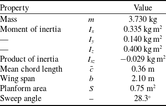




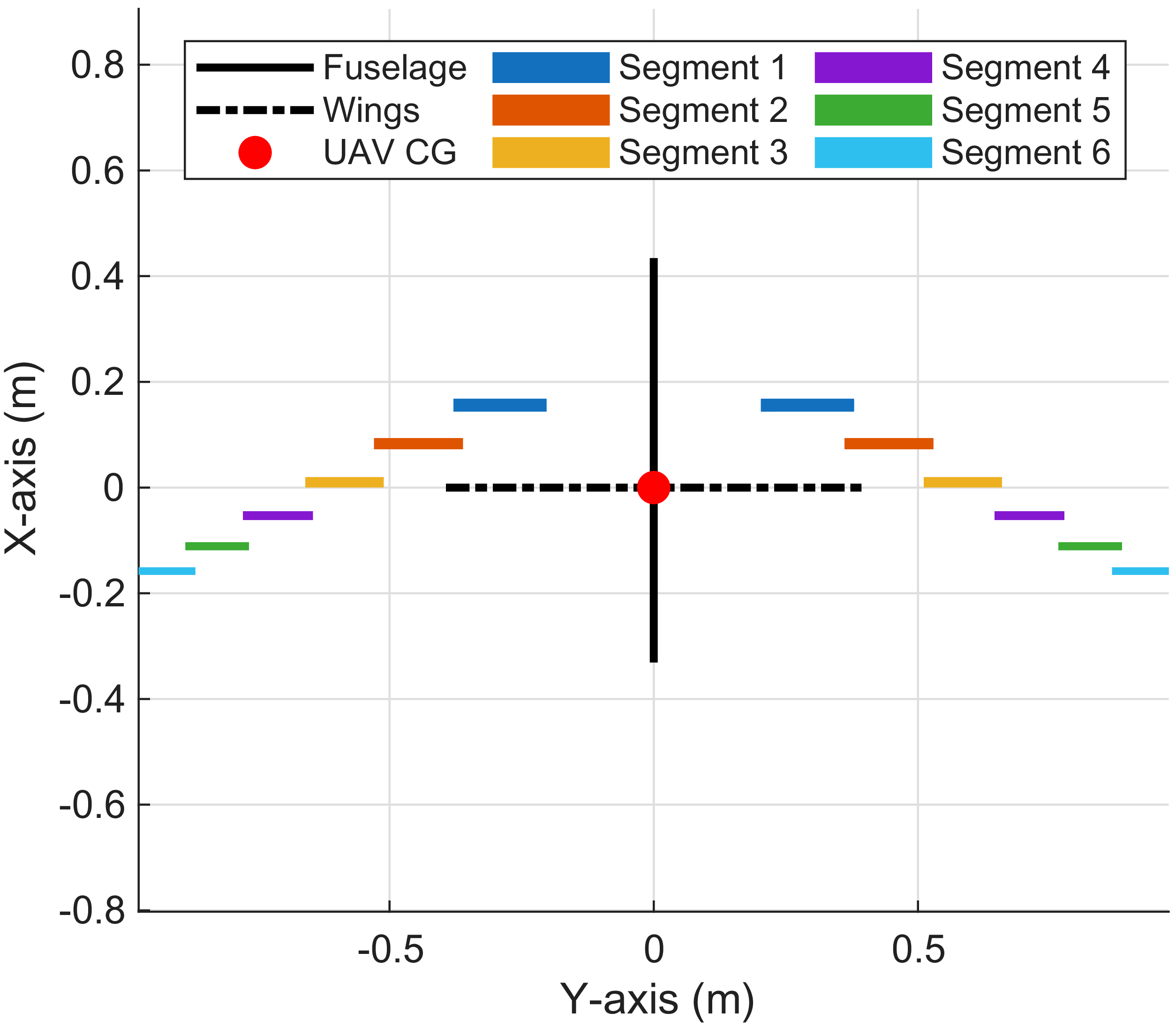
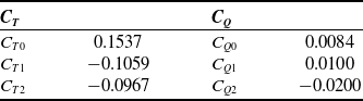
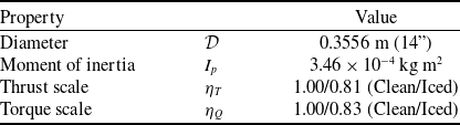

 2nd

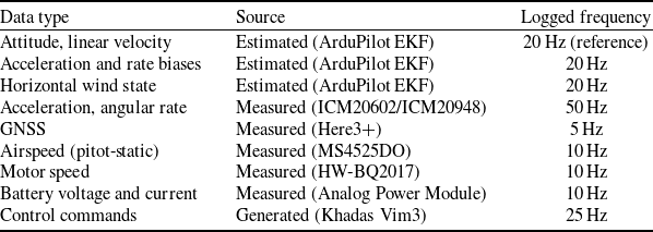
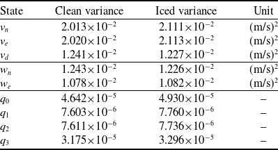




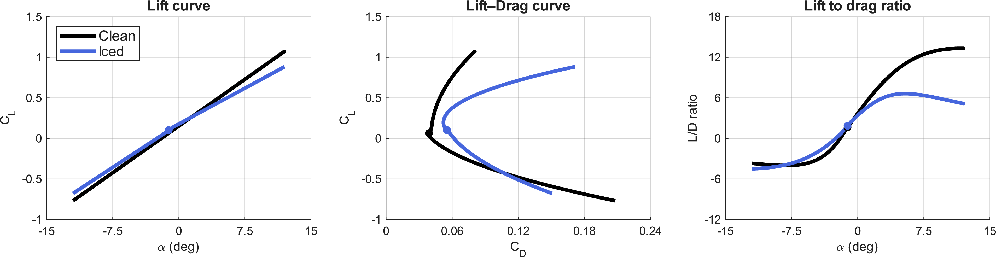
 δe=q=0
 α0=−0.02rad


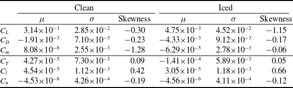

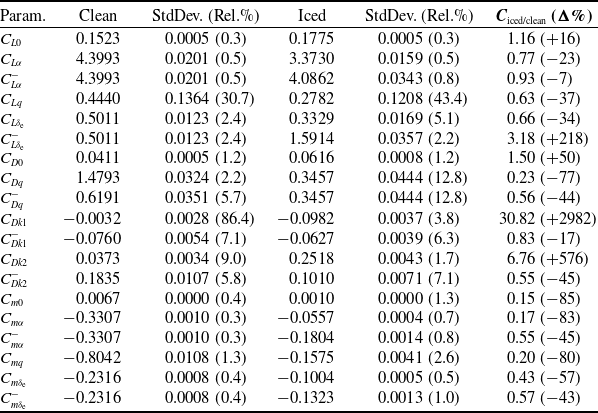
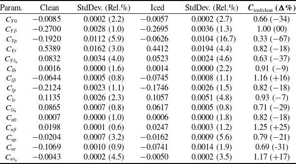
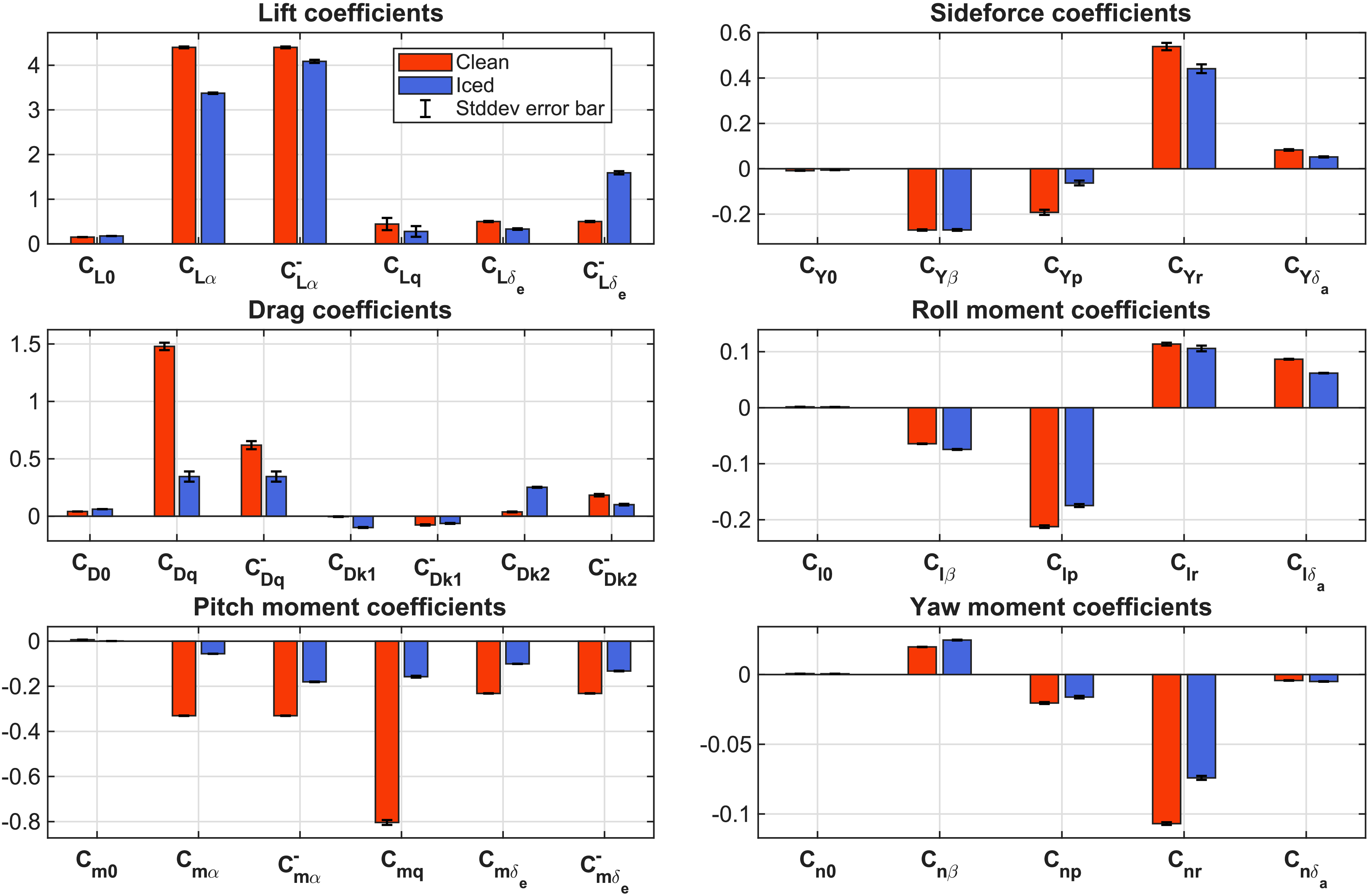
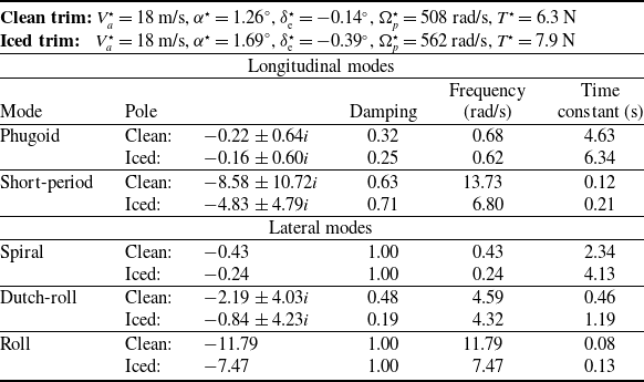
 Va=18m/s


 Va=18m/s

 Open access

