2.1 Elements of differential geometry

In this subsection, we focus on fundamentals of differential geometry. We consider fluid motion on an $n$ -dimensional manifold $M$ which at this point does not have to be equipped with a metric. The manifold $M$ is taken to be fixed, that is, time independent, and to have fixed boundary $\unicode[STIX]{x2202}M$ (which could be empty). Free-surface effects are therefore ignored, though they could be incorporated in essentially the same formalism. Obvious examples of manifolds $M$ of interest are the Euclidean space $\mathbb{R}^{n}$ , with $n=2,3$ , the torus $\mathbb{T}^{n}$ , the 2-sphere $\mathbb{S}^{2}\subset \mathbb{R}^{3}$ given by $r=1$ and the spherical shells $r_{0}\leqslant r\leqslant r_{1}$ in $\mathbb{R}^{3}$ , where $r$ is the radial component of spherical polar coordinates. We treat $M$ in a coordinate-independent way but, since we deal with non-relativistic fluids, retain the special role of the time coordinate $t$ .

The basic object in fluid mechanics, and more generally in continuum mechanics, is the flow map, $\unicode[STIX]{x1D719}_{t}$ , which maps the positions of fluid particles at the initial time $t=0$ to their positions at time $t$ . Thus, if $x$ denotes the position at time $t$ of the particle initially at $a$ ,

The flow map is a diffeomorphism, that is, a smooth invertible map from $M$ to itself. We write $\unicode[STIX]{x1D719}_{t}:M\rightarrow M$ and $\unicode[STIX]{x1D719}_{t}\in \text{Diff}(M)$ , where $\text{Diff}(M)$ is the set of all diffeomorphisms from $M$ to $M$ . We shall be mostly be concerned with the subset $\text{SDiff}(M)$ of $\text{Diff}(M)$ consisting of all the volume-preserving diffeomorphisms from $M$ to $M$ . For convenience, we generally omit the subscript $t$ from the flow map in what follows, simply remembering that $\unicode[STIX]{x1D719}$ depends on time, as essentially do most of the objects introduced. Being fixed, the boundary $\unicode[STIX]{x2202}M$ is preserved under the action of any flow map $\unicode[STIX]{x1D719}$ ; if it has more than one connected component, $\unicode[STIX]{x1D719}$ must map each component to itself, otherwise $\unicode[STIX]{x1D719}$ would be not be continuously connected to the identity map, the flow map at $t=0$ .

In the standard Eulerian description of fluids, $\unicode[STIX]{x1D719}$ does not appear explicitly; instead, it is the velocity field $u=u(\cdot )$ that appears as the fundamental dynamical variable. It is defined by

where the overdot denotes time derivative and $a\in M$ is arbitrary. Equivalently,

where $\circ$ denotes composition. In writing (2.2) we have adhered to our convention of omitting to make explicit the time dependence of $u$ on $t$ . When the velocity field is known, the flow map is deduced by integrating the ordinary differential equations (2.2) with the initial condition $\unicode[STIX]{x1D719}|_{t=0}=\text{id}$ , that is, the identity map.

Figure 1.

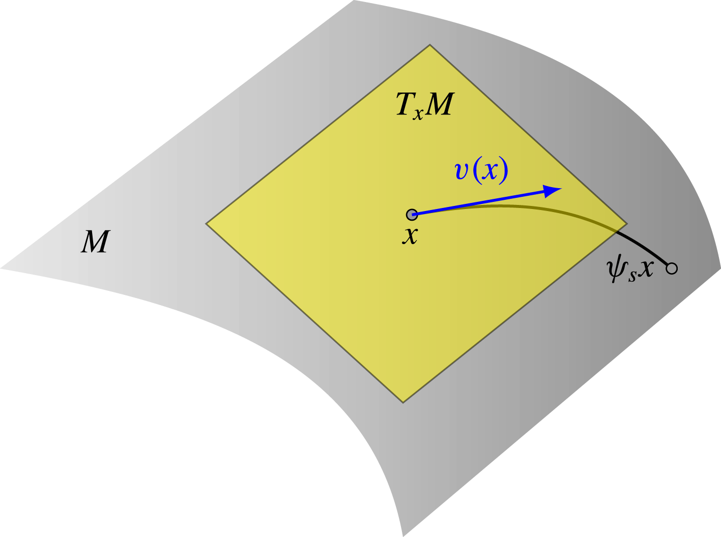
A vector $v(x)$ in the tangent space $T_{x}M$ at $x\in M$ is defined by a curve $\unicode[STIX]{x1D713}_{s}x$ according to (2.4).

The velocity field is an example of a vector field on $M$ . In general, a vector at $x$ such as $v(x)$ can be identified as an equivalence class of curves through $x\in M$ sharing the same tangent. If $\unicode[STIX]{x1D713}_{s}x$ is one such curve parameterised by $s$ and with $\unicode[STIX]{x1D713}_{0}x=x$ , we write that

where $T_{x}M$ is the tangent space to $M$ at $x$ (the set of all vectors at $x$ ). This formalises the interpretation of vectors as displacements – arrows – between two infinitesimally close points $x$ and $y=\unicode[STIX]{x1D713}_{s}x$ with $s\rightarrow 0$ , as illustrated in figure 1. (Note that (2.2) is an instance of (2.4) with $\unicode[STIX]{x1D713}_{s}=\unicode[STIX]{x1D719}_{t+s}$ .) A vector field, then, is a map $v$ from $M$ to the tangent bundle $TM$ (the union of the tangent spaces $T_{x}M$ at all points $x\in M$ ) with the property that $v(x)\in T_{x}M$ . We emphasise this property because traditional GLM formulations involve objects such as $u\circ \unicode[STIX]{x1D719}$ which are not vector fields (since $(u\circ \unicode[STIX]{x1D719})(x)=u(\unicode[STIX]{x1D719}x)\in T_{\unicode[STIX]{x1D719}x}M\not =T_{x}M$ ) and, in our opinion, are best avoided for clarity in a general setting. Note that if $M$ has a fixed boundary $\unicode[STIX]{x2202}M$ , the velocity field is tangential to it, $u\Vert \unicode[STIX]{x2202}M$ (meaning that $u(x)\in T_{x}\unicode[STIX]{x2202}M$ for boundary points $x\in \unicode[STIX]{x2202}M$ ).

Fluid dynamics on arbitrary manifolds is formulated most naturally using fields of differential one-forms in addition to vector fields. A one-form at $x$ is defined as a linear map from vectors in $T_{x}M$ to the real numbers. One-forms at $x$ make up a vector space, the cotangent space $T_{x}^{\ast }M$ , and their application to vectors of $T_{x}M$ is interpreted as a pairing (or interior product) which produces a real number. If $v$ is a vector field on $M$ and $\unicode[STIX]{x1D708}$ is a field of one-forms, the pairing at $x$ is denoted as

and defines a scalar field, a real function over the whole manifold $M$ . In coordinates, with $v^{i}(x)$ and $\unicode[STIX]{x1D708}_{i}(x)$ denoting the components of the vector and one-form, the pairing (2.5) is simply given by $\unicode[STIX]{x1D708}(v)=v^{i}\unicode[STIX]{x1D708}_{i}$ at each point $x$ . Note that the coordinates $x^{i}$ need not be orthogonal; indeed ‘orthogonality’ is meaningless since no metric has yet been introduced. Pictorially, one-forms can be represented as stacks of infinitesimally close planes (in dimension $n=3$ ; hyperplanes of dimension $n-1$ in general) and their pairing with a vector interpreted as measuring the number of planes pierced by the vector. (Note that, although we will not adopt this terminology, vectors such as $v(x)$ are traditionally referred to as ‘contravariant vectors’ and one-forms such as $\unicode[STIX]{x1D708}(x)$ as ‘covariant vectors’, and their pairing as ‘contraction’.)

Higher-order forms (and fields thereof) are defined similarly as linear maps on sets of vectors, with added skew-symmetry properties: a $k$ -form $\unicode[STIX]{x1D6FC}$ acts linearly on $k$ vectors $v_{1},\ldots ,v_{k}$ to produce the real number $\unicode[STIX]{x1D6FC}(v_{1},\ldots ,v_{k})$ which is invariant under even permutations of its arguments and flips signs under odd permutations. For example, a two-form $\unicode[STIX]{x1D6FC}$ acts linearly on pairs of vectors $u$ , $v$ , with $\unicode[STIX]{x1D6FC}(u,v)=-\unicode[STIX]{x1D6FC}(v,u)\in \mathbb{R}$ ; in coordinates, it has components $\unicode[STIX]{x1D6FC}_{ij}$ that are anti-symmetric, $\unicode[STIX]{x1D6FC}_{ij}=-\unicode[STIX]{x1D6FC}_{ji}$ , and satisfy $\unicode[STIX]{x1D6FC}(u,v)=\unicode[STIX]{x1D6FC}_{ij}u^{i}v^{j}$ . Zero-forms are simply scalars. For an $n$ -dimensional $M$ , the set of $k$ -forms makes up a vector space of dimension $\binom{n}{k}$ , so that all $n$ -forms are scalar multiples of one another and therefore proportional to a reference $n$ -form, termed the ‘volume-form’ and denoted by $\unicode[STIX]{x1D714}$ . Differential forms may be naturally integrated, along curves for one-forms, surfaces for two-forms, etc. (e.g. Schutz Reference Schutz1980; Frankel Reference Frankel1997). The wedge (or exterior) product $\wedge$ combines a $k$ -form $\unicode[STIX]{x1D6FC}$ with an $l$ -form $\unicode[STIX]{x1D6FD}$ to produce a $(k+l)$ -form $\unicode[STIX]{x1D6FC}\wedge \unicode[STIX]{x1D6FD}$ and is defined as an anti-symmetrised tensor product.

Figure 2.

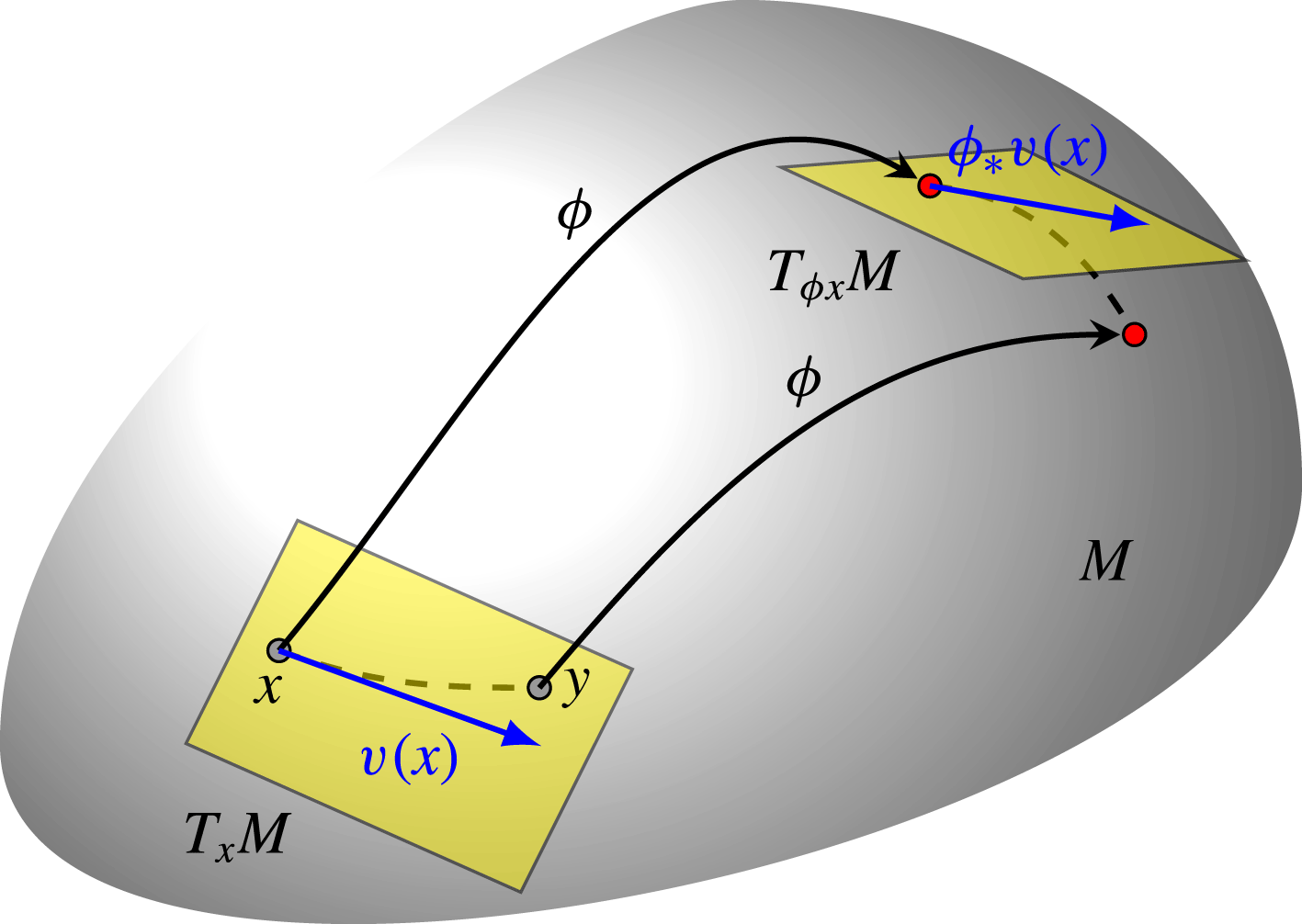
Push-forward of a vector $v(x)$ at $x$ : a curve $\unicode[STIX]{x1D713}_{s}x$ tangent to $v(x)$ at $x$ (dashed line) which includes a point $y$ is mapped to a curve passing through $\unicode[STIX]{x1D719}x$ and $\unicode[STIX]{x1D719}y$ . The tangent of the latter curve at $\unicode[STIX]{x1D719}x$ defines the push-forward $\unicode[STIX]{x1D719}_{\ast }v(x)$ .

The geometric tools used in this paper include the push-forward and pull-back of vectors and differential forms (and indeed any tensor) by diffeomorphisms such as the flow map. The definition of the push-forward $\unicode[STIX]{x1D719}_{\ast }$ by a map $\unicode[STIX]{x1D719}:M\rightarrow M$ recognises that the action of diffeomorphisms on points naturally induces an action on vectors thought of as infinitesimal displacements. The push-forward $\unicode[STIX]{x1D719}_{\ast }v(x)\in T_{\unicode[STIX]{x1D719}x}M$ of $v(x)$ is a vector at the image point $\unicode[STIX]{x1D719}x$ defined as the tangent to the curve $\unicode[STIX]{x1D719}(\unicode[STIX]{x1D713}_{s}x)$ , with $\unicode[STIX]{x1D713}_{s}x$ a curve tangent to $v$ at $x$ to satisfy (2.4); explicitly, we have

see figure 2. The push-forward $\unicode[STIX]{x1D719}_{\ast }$ , often termed the differential of $\unicode[STIX]{x1D719}$ , is linear. It provides a way to map entire vector fields $v$ according to

and arises naturally in applications of the chain rule, for example in (3.3) below. In coordinates $x^{i}$ , the push-forward takes the form

A well-known example of the push-forward of a vector field arises in MHD with the observation that, for incompressible flow in the absence of diffusion, the magnetic field is a ‘frozen’ vector field, transported by the flow according to the Cauchy solution. The magnetic field $b$ at any $t$ is then the push-forward of the initial magnetic field $b_{0}$ by the volume-preserving flow map: $b=\unicode[STIX]{x1D719}_{\ast }b_{0}$ .

Once the push-forward of a vector is defined, the definitions of the push-forward and pull-back of various tensors follow naturally. The pull-back $\unicode[STIX]{x1D719}^{\ast }$ of a vector $v(x)\in T_{x}M$ by $\unicode[STIX]{x1D719}$ is simply the push-forward under the inverse map $\unicode[STIX]{x1D719}^{-1}$ , that is,

using the invertibility of the diffeomorphism. The pull-back of one-forms is defined using their duality with vectors: if $\unicode[STIX]{x1D708}(x)\in T_{x}^{\ast }M$ is a one-form, its pull-back $\unicode[STIX]{x1D719}^{\ast }\unicode[STIX]{x1D708}(x)\in T_{\unicode[STIX]{x1D719}^{-1}x}^{\ast }M$ satisfies

With this definition, the coordinate expression of the pull-back of a one-form field $\unicode[STIX]{x1D708}=\unicode[STIX]{x1D708}_{i}\,\text{d}x^{i}$ is readily obtained from (2.8) as

The pull-back of other differential forms is defined similarly via pairing with vectors; the push-forward is defined as the pull-back by the inverse map in a way that mirrors (2.9). Note that the pull-back and push-forward of scalar functions (zero-forms) are simple compositions: $\unicode[STIX]{x1D719}^{\ast }f=f\circ \unicode[STIX]{x1D719}$ and $\unicode[STIX]{x1D719}_{\ast }f=f\circ \unicode[STIX]{x1D719}^{-1}$ .

Another important differential-geometric tool is the Lie derivative with respect to a vector field $v$ . For any tensor field (vector or form) $\unicode[STIX]{x1D70F}$ , the Lie derivative is defined by

where the map $\unicode[STIX]{x1D713}_{s}$ is the flow of $v$ in the sense that

An application to the fluid flow map $\unicode[STIX]{x1D719}$ and associated (time-dependent) vector field $u$ gives the useful formula

holding when $\unicode[STIX]{x1D70F}$ depends explicitly on $t$ . Another useful property concerns the action of pull-back on Lie derivatives: for any vector field $v$ ,

Both properties (2.14) and (2.15) are derived in § A.1, and in Soward & Roberts (Reference Soward and Roberts2010, Reference Soward and Roberts2014) using coordinate methods. Coordinate expressions for Lie derivatives are obtained by writing the map $\unicode[STIX]{x1D713}_{s}$ in (2.12) as $(\unicode[STIX]{x1D713}_{s}x)^{i}=x^{i}+sv^{i}(x)+o(s)$ and using the coordinate expression of the pull-back. This gives

for the Lie derivatives of scalar fields $f$ (zero-forms), vector fields $v$ and one-form fields $\unicode[STIX]{x1D708}$ , respectively. An interpretation of the Lie derivative of a vector field is used repeatedly in what follows: if a map $\unicode[STIX]{x1D713}_{s,t}$ depends on the two parameters $s$ and $t$ , we can define the two $s$ - and $t$ -dependent vector fields

in the manner of (2.2). The Lie derivative of $v$ with respect to $u$ then satisfies

The final operation needed in what follows is the exterior derivative $\text{d}$ which acts on a $k$ -form field to produce a $(k+1)$ -form field. It is defined by its action on a scalar field $f$ , giving a one-form field $\text{d}f$ with the property that $(\text{d}f)(v)={\mathcal{L}}_{v}f$ for any vector field $v$ , by the property that $\text{d}^{2}\unicode[STIX]{x1D6FC}=0$ for any form $\unicode[STIX]{x1D6FC}$ , and by its action on the exterior (wedge) products of forms, $\text{d}(\unicode[STIX]{x1D6FC}\wedge \unicode[STIX]{x1D6FD})=\text{d}\unicode[STIX]{x1D6FC}\wedge \unicode[STIX]{x1D6FD}+(-1)^{k}\unicode[STIX]{x1D6FC}\wedge \text{d}\unicode[STIX]{x1D6FD}$ where $\unicode[STIX]{x1D6FC}$ is a $k$ -form. For our purpose, an important property of the exterior derivative is that it commutes with pull-backs/push-forwards by diffeomorphisms and with Lie derivatives:

Another is Cartan’s formula

relating the Lie derivative of a $k$ -form $\unicode[STIX]{x1D6FC}$ to its exterior derivative by means of the interior product $\unicode[STIX]{x1D704}_{v}\unicode[STIX]{x1D6FC}$ defined as the $(k-1)$ -form such that $(\unicode[STIX]{x1D704}_{v}\unicode[STIX]{x1D6FC})(v_{1},\!\ldots \,,v_{k-1})=\unicode[STIX]{x1D6FC}(v,v_{1},\ldots ,v_{k-1})$ for all vectors $v_{1},\ldots ,v_{k-1}$ .

2.2 Fluid dynamics on a Riemannian manifold

We now review the geometric formulation of fluid dynamics which naturally emerges from Arnold’s (Reference Arnold1966) interpretation of the motion of a perfect incompressible fluid on an arbitrary manifold as geodesic motion (see also Ebin & Marsden Reference Ebin and Marsden1970; Arnold & Khesin Reference Arnold and Khesin1998; Holm, Marsden & Ratiu Reference Holm, Marsden and Ratiu1998). This requires the manifold $M$ to have a Riemannian structure, that is, to be equipped with a metric $g(\cdot ,\cdot )$ , a positive-definite bilinear form which, at each point $x\in M$ , maps pairs of vectors to non-negative real numbers, thus generalising the scalar product of Euclidean space. The metric induces a preferred $n$ -form, which we take as the reference volume form $\unicode[STIX]{x1D714}$ . This volume form defines the volume element on $M$ and appears naturally in integrals over the domain such as $\int _{M}f\unicode[STIX]{x1D714}$ where $f$ is a scalar function. A fluid motion is incompressible provided the associated flow map $\unicode[STIX]{x1D719}$ preserves volume in the sense that

This is the explicit form of $\unicode[STIX]{x1D719}\in \text{SDiff}(M)\subset \text{Diff}(M)$ .

The metric $g$ induces a distance $d(x,y)$ between points $x$ and $y$ on $M$ . This is the length of the shortest path from $x$ to $y$ , which is defined by

where $\unicode[STIX]{x1D6FE}_{s}$ denotes paths joining $x$ and $y$ , and the prime denotes an $s$ -derivative. The distance here does not depend on the parameterisation of the path, including the choice of interval $[0,S]$ . It is then a standard result that obtaining $d(x,y)$ by the above variational principle is equivalent to a more convenient formula for the distance squared,

Here the parameterisation is no longer arbitrary, and the minimising path $\unicode[STIX]{x1D6FE}_{s}$ is characterised by a constant kinetic energy $g(\unicode[STIX]{x1D6FE}_{s}^{\prime },\unicode[STIX]{x1D6FE}_{s}^{\prime })/2$ . We refer the reader to Arnold & Khesin (Reference Arnold and Khesin1998) for more discussion; we write other types of distances using formulae of the type (2.23) in what follows without further comment.

The distance $d(x,y)$ in (2.22) or (2.23) between points in $M$ does not play an immediate role in the dynamics of fluids on $M$ . The key role is rather played by the distance between two points in $\text{SDiff}(M)$ , that is, between pairs of volume-preserving diffeomorphisms $\unicode[STIX]{x1D719},\unicode[STIX]{x1D713}$ . This distance is defined by

where $\unicode[STIX]{x1D6FE}_{s}$ now denotes paths joining $\unicode[STIX]{x1D719}$ to $\unicode[STIX]{x1D713}$ in $\text{SDiff}(M)$ . Introducing the $s$ -dependent vector field $q=\unicode[STIX]{x1D6FE}_{s}^{\prime }\circ \unicode[STIX]{x1D6FE}_{s}^{-1}$ and using volume preservation, this can be rewritten as

This makes explicit the right invariance of the metric associated with $D^{2}$ , that is, the invariance of the integral over $M$ in (2.24) with respect to the right translations $\unicode[STIX]{x1D6FE}_{s}\mapsto \unicode[STIX]{x1D6FE}_{s}\circ \unicode[STIX]{x1D712}$ for an arbitrary $s$ -independent $\unicode[STIX]{x1D712}\in \text{SDiff}(M)$ . This invariance implies that $D(\unicode[STIX]{x1D719},\unicode[STIX]{x1D713})=D(\unicode[STIX]{x1D719}\circ \unicode[STIX]{x1D713}^{-1},\text{id})$ . In physical terms, $D^{2}$ is twice the $s$ -integrated kinetic energy for a flow that joins the two configurations $\unicode[STIX]{x1D713}$ and $\unicode[STIX]{x1D719}$ of the fluid.

The geometric view of the Euler equations for an incompressible perfect fluid on $M$ is that they arise as geodesic equations on $\text{SDiff}(M)$ equipped with the distance (2.25). Specifically, the Euler equations are obtained by minimising the action

over all time-dependent flow maps $\unicode[STIX]{x1D719}\in \text{SDiff}(M)$ (with corresponding velocity $u=\dot{\unicode[STIX]{x1D719}}\circ \unicode[STIX]{x1D719}^{-1}$ ) which join two fixed flow maps between $t=0$ and $t=T$ . The motion which achieves the minimum is an incompressible flow with constant kinetic energy. When the Euler equations are derived in this fashion, the natural dynamical variable is not the velocity field $u=\dot{\unicode[STIX]{x1D719}}\circ \unicode[STIX]{x1D719}^{-1}$ but the momentum conjugate to it, that is, the one-form $\unicode[STIX]{x1D708}$ obtained from $u$ using the metric $g$ according to

say, meaning that $\unicode[STIX]{x1D708}(v)=g(u,v)$ for all $v\in T_{x}M$ . Equation (2.27) defines the so-called inertia operator which associates a one-form such as $\unicode[STIX]{x1D708}$ to a vector such as $u$ ; we say that $\unicode[STIX]{x1D708}$ is dual to $u$ . In coordinates (2.27) amounts to the familiar lowering of an index: $\unicode[STIX]{x1D708}_{i}=g_{ij}u^{j}$ . This observation motivates the musical notation $u_{\flat }$ (and its inverse $\unicode[STIX]{x1D708}_{\sharp }$ ). The one-form (2.27) dual to the velocity field will be called the ‘momentum one-form’.

Minimising the action $\mathscr{A}$ in (2.26) leads to the Euler equations in the form

where $\unicode[STIX]{x1D70B}$ is a Lagrange multiplier enforcing volume preservation and $\operatorname{div}u$ is defined by ${\mathcal{L}}_{u}\unicode[STIX]{x1D714}=(\operatorname{div}u)\unicode[STIX]{x1D714}$ (see appendix B for a derivation, and Holm, Marsden & Ratiu (Reference Holm, Marsden and Ratiu1998) for a general formulation applicable to a broad class of fluid models). In this derivation, $\unicode[STIX]{x1D708}$ appears as the variational derivative of the Lagrangian $\int _{M}g(u,u)\unicode[STIX]{x1D714}$ with respect to $u$ , hence its interpretation as the conjugate momentum, noted above. Applying the metric, (2.28) can be rewritten in terms of the vector field $u=\unicode[STIX]{x1D708}_{\sharp }$ as

where $p=\unicode[STIX]{x1D70B}+g(u,u)/2$ is the usual pressure, $\unicode[STIX]{x1D735}p=(\text{d}p)_{\sharp }$ and $\unicode[STIX]{x1D735}_{u}$ is the covariant derivative based on $g$ (see (2.36) below for a coordinate expression). The derivation of (2.29) uses the identity

(e.g. Arnold & Khesin Reference Arnold and Khesin1998, Theorem IV.1.17). While (2.29) may have the more familiar form, (2.28) turns out to be superior in the context of GLM theories. Its advantages are hinted at by the ease with which Kelvin’s circulation theorem follows, as we now show. Using (2.14) and (2.19), (2.28) can be rewritten as

Now, let $C_{0}\subset M$ be a closed curve in the initial fluid configuration and $\unicode[STIX]{x1D719}C_{0}$ its image as deformed under the flow map $\unicode[STIX]{x1D719}$ , then

This shows that the circulation around any material curve

The vorticity is the two-form $\text{d}\unicode[STIX]{x1D708}$ . It is transported by the flow: taking the exterior derivative $\text{d}$ of (2.28) and using that $\text{d}^{2}=0$ gives the vorticity equation

This means that vorticity is pushed forward by the flow map from the initial condition, $\text{d}\unicode[STIX]{x1D708}=\unicode[STIX]{x1D719}_{\ast }\,\text{d}\unicode[STIX]{x1D708}|_{t=0}$ ; see Besse & Frisch (Reference Besse and Frisch2017) for discussion of this and applications to helicity.

For completeness, we record the coordinate version of (2.28) and (2.29). Using (2.16), (2.28) is written explicitly as

where the expression for the divergence is obtained using that $\unicode[STIX]{x1D714}=|g|^{1/2}\,\text{d}x^{1}\wedge \text{d}x^{2}\wedge \cdots \wedge \text{d}x^{n}$ , with $|g|$ the determinant of $g_{ij}$ . Introducing $\unicode[STIX]{x1D708}_{i}=g_{ij}u^{j}$ into the first equation of (2.35) leads after a short computation to

where $\unicode[STIX]{x1D6E4}_{jk}^{i}=g^{il}(\unicode[STIX]{x2202}_{j}g_{lk}+\unicode[STIX]{x2202}_{k}g_{lj}-\unicode[STIX]{x2202}_{l}g_{jk})/2$ is the Christoffel symbol (Hawking & Ellis Reference Hawking and Ellis1973; Schutz Reference Schutz1980). This is the coordinate version of (2.29).

2.3 Other fluid models

To conclude this section we note that more complicated fluids than the perfect incompressible fluids considered so far are governed by equations that have a structure similar to that of the Euler equations. The three-dimensional ( $n=3$ ) Boussinesq equations are widely used to model rotating–stratified geophysical fluids. In coordinate-free notation, they take the form

where $\unicode[STIX]{x1D703}$ is the buoyancy acceleration, $\unicode[STIX]{x1D6F7}$ the geopotential divided by $g$ , given by $z$ in the Euclidean case, and $\unicode[STIX]{x1D708}_{a}$ is the absolute momentum one-form

Here $A$ is a one-form that encodes planetary rotation; on the $f$ -plane, with $f$ the constant Coriolis parameter and in Cartesian coordinates, it is given by

up to an irrelevant differential. Like the Euler equations, the Boussinesq equations have a variational formulation: (2.37) may be obtained by minimising the action

over time-dependent flow maps $\unicode[STIX]{x1D719}$ and with $\unicode[STIX]{x1D703}=\unicode[STIX]{x1D719}_{\ast }\unicode[STIX]{x1D703}_{0}$ transported from its initial value (e.g. Holm, Marsden & Ratiu Reference Holm, Marsden and Ratiu1998).

Taking the exterior derivatives of (2.37a ) and (2.37b ) gives

The two-form $\text{d}\unicode[STIX]{x1D708}_{a}$ corresponds to the absolute vorticity. The conservation

of the potential-vorticity three-form

follows immediately. The more familiar scalar Rossby–Ertel potential vorticity $Q$ is defined by $Q\unicode[STIX]{x1D714}={\mathcal{Q}}$ and is also conserved: $(\unicode[STIX]{x2202}_{t}+{\mathcal{L}}_{u})Q=0$ . We note that ${\mathcal{Q}}$ can be interpreted as the mass of Haynes & McIntyre’s (Reference Haynes and McIntyre1987) potential-vorticity substance and its impermeability property related to the alternative form ${\mathcal{Q}}=\text{d}(\unicode[STIX]{x1D708}_{a}\wedge \text{d}\unicode[STIX]{x1D703})$ (see also Haynes & McIntyre Reference Haynes and McIntyre1990; Bretherton & Schär Reference Bretherton and Schär1993).

Similarly, a perfect compressible fluid, with equation of state $p=P(\unicode[STIX]{x1D70C},\unicode[STIX]{x1D703})$ , where $\unicode[STIX]{x1D70C}$ and $\unicode[STIX]{x1D703}$ are the density and entropy, is governed by the equations

Here the mass $m$ is defined as the $n$ -form $m=\unicode[STIX]{x1D70C}\unicode[STIX]{x1D714}$ , so that (2.44b ) is equivalent to the continuity equation $\unicode[STIX]{x2202}_{t}\unicode[STIX]{x1D70C}+\operatorname{div}(\unicode[STIX]{x1D70C}u)=0$ . The conservation

of the potential-vorticity three-form $\text{d}\unicode[STIX]{x1D708}\wedge \text{d}\unicode[STIX]{x1D703}$ follows from observing that $\text{d}p\wedge \text{d}\unicode[STIX]{x1D70C}\wedge \text{d}\unicode[STIX]{x1D703}=0$ by virtue of the dependence $p=p(\unicode[STIX]{x1D70C},\unicode[STIX]{x1D703})$ . In three dimensions, $n=3$ , the more usual scalar Rossby–Ertel potential vorticity $Q$ is defined by the relation $Qm=\text{d}\unicode[STIX]{x1D708}\wedge \text{d}\unicode[STIX]{x1D703}$ (Schutz Reference Schutz1980). Its conservation (as a scalar) is an immediate consequence of the conservation of the two three-forms $\text{d}\unicode[STIX]{x1D708}\wedge \text{d}\unicode[STIX]{x1D703}$ and $m$ .

Finally, we formulate the equations governing the dynamics of ideal MHD flows in a coordinate-free way, in $n=3$ dimensions (e.g. Frankel Reference Frankel1997). We let $b$ be the magnetic (vector) field, $\unicode[STIX]{x1D6FD}=g(b,\cdot )=b_{\flat }$ its dual one-form, and the flux two-form $B$ be defined by the interior product $\unicode[STIX]{x1D704}_{b}\unicode[STIX]{x1D714}=\unicode[STIX]{x1D714}(b,\cdot ,\cdot )=B$ . The condition that the magnetic field be divergence free, $\operatorname{div}b=0$ , amounts to requiring that $\text{d}B=0$ (the two-form $B$ is said to be closed). This is preserved under the induction equation, which is simply transport of $B$ by the flow $u$ ,

The corresponding equation for magnetic field is then

This extra term ensures that $b$ remains divergence free and means that $b$ is transported as a ‘tensor of weight $-1$ ’, as is density $\unicode[STIX]{x1D70C}$ (see below (2.44)). We will not use the machinery of tensor weights in this paper; see the parallel development in Soward & Roberts (Reference Soward and Roberts2014) and note that if the flow is incompressible, $\operatorname{div}u=0$ and $b$ is transported as a vector field.

The momentum equation may be written, in general, as

The two versions of the Lorentz force term are linked by the Cartan formula, giving here ${\mathcal{L}}_{b}\unicode[STIX]{x1D6FD}=\unicode[STIX]{x1D704}_{b}\,\text{d}\unicode[STIX]{x1D6FD}+\text{d}(\unicode[STIX]{x1D704}_{b}\unicode[STIX]{x1D6FD})$ . Compressible MHD is governed then by (2.46) or (2.47), (2.48), conservation of mass (2.44b ) and an equation of state such as $p=P(\unicode[STIX]{x1D70C})$ . Note that the Lorentz force term involves both the magnetic (vector) field $b$ and the corresponding one-form $\unicode[STIX]{x1D6FD}$ as discussed by Holm (Reference Holm2002b ) and Roberts & Soward (Reference Roberts and Soward2006a ).

3.1 Generalising GLM to arbitrary manifolds

GLM and other Lagrangian-mean theories can be thought of as extensions to $\text{SDiff}(M)$ of the classical (Krylov–Bogoliubov–Mitropolsky) averaging of ordinary differential equations (e.g. Nayfeh Reference Nayfeh1973; Sanders & Verhulst Reference Sanders and Verhulst1985). The central idea is to seek a variable transformation that represents the state of the system as the sum of a mean position and a perturbation. Crucially the mean is defined, if possible, in such a way that the perturbation remains bounded and small for long times, so that the fluctuating states stay close to the mean state. The mean dynamics is of course affected by the perturbation; as a result, the equations governing the mean dynamics contain terms representing the average effect of the perturbation. Often these terms depend only on a few features of the perturbation so there is no need to work out all the details of its evolution.

In a similar manner, in GLM one wishes to define a mean configuration of the fluid – a mean flow map $\bar{\unicode[STIX]{x1D719}}$ – that stays close to the exact fluctuating flow maps but evolves in a simpler manner because it filters out fluctuations. The theory applies to different types of averaging: the fast-time averaging that appears in asymptotic treatments of two-time-scale models, averaging along a particular direction, or a probabilistic average when fluctuations model uncertainty. For this reason it is customary since Andrews & McIntyre (Reference Andrews and McIntyre1978a ) to develop GLM theories for an arbitrary ensemble average, only stipulating the ensemble when applications are made specific. We follow this approach and consider an ensemble of flow maps $\unicode[STIX]{x1D719}^{\unicode[STIX]{x1D6FC}}$ , where the parameter $\unicode[STIX]{x1D6FC}$ indexes the ensemble. It is useful to think of $\unicode[STIX]{x1D6FC}$ taking a few integer values, with the ensemble consisting of a few different flows, or real values, so that the ensemble consists of a one-parameter family of flows. The theory is not restricted to these cases however and applies to the most general situation when the ensemble is determined by specifying a measure on $\text{SDiff}(M)$ .

Figure 3.

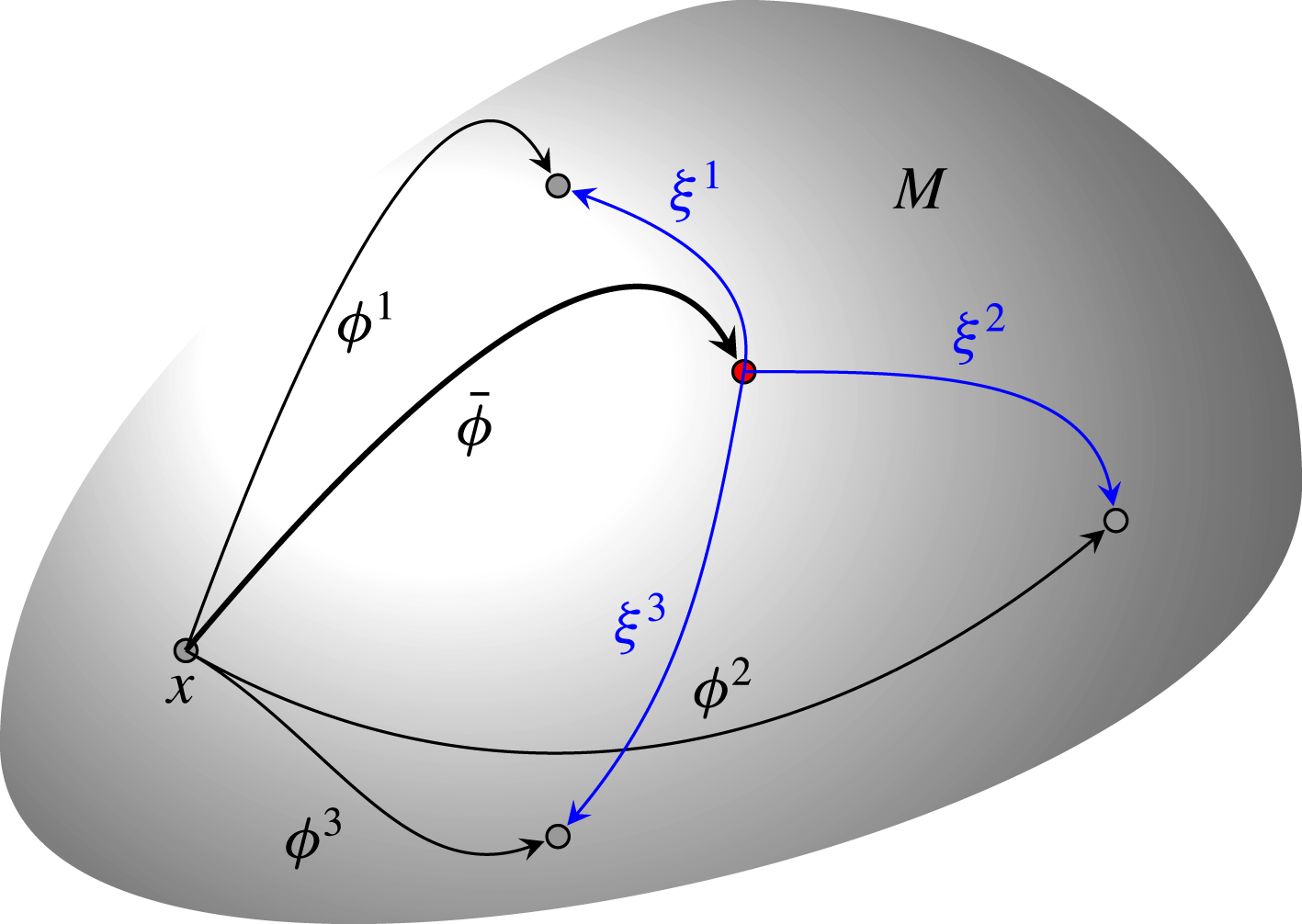
Decomposition $\unicode[STIX]{x1D719}^{\unicode[STIX]{x1D6FC}}=\unicode[STIX]{x1D709}^{\unicode[STIX]{x1D6FC}}\circ \bar{\unicode[STIX]{x1D719}}$ of the flow maps shown acting on a single point $x\in M$ .

It is natural to write each fluctuating flow map $\unicode[STIX]{x1D719}^{\unicode[STIX]{x1D6FC}}$ in the ensemble as the composition

of a perturbation map $\unicode[STIX]{x1D709}^{\unicode[STIX]{x1D6FC}}$ with a mean flow map $\bar{\unicode[STIX]{x1D719}}$ . The maps $\unicode[STIX]{x1D719}^{\unicode[STIX]{x1D6FC}}$ then stay close to $\bar{\unicode[STIX]{x1D719}}$ when the maps $\unicode[STIX]{x1D709}^{\unicode[STIX]{x1D6FC}}$ stay close to the identity. Expression (3.1) was used, for example, by Holm (Reference Holm2002a ,Reference Holm b ) and Marsden & Shkoller (Reference Marsden and Shkoller2003), and naturally extends to arbitrary manifolds the sum $\boldsymbol{x}$ + $\unicode[STIX]{x1D743}(\boldsymbol{x},t)$ of mean position $\boldsymbol{x}$ and perturbation $\unicode[STIX]{x1D743}(\boldsymbol{x},t)$ of standard GLM. 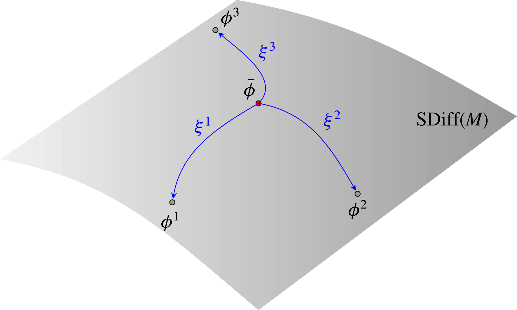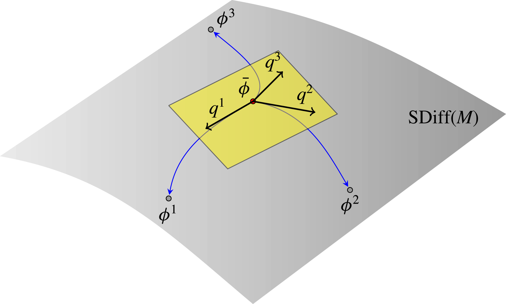It can be visualised either by thinking of the decomposition of $\unicode[STIX]{x1D719}^{\unicode[STIX]{x1D6FC}}x$ for a particular point $x\in M$ (see figure 3), or by thinking of $\unicode[STIX]{x1D719}^{\unicode[STIX]{x1D6FC}}$ as a point on the infinite-dimensional manifold $\text{SDiff}(M)$ (see figure 4). Note that we do not insist that $\unicode[STIX]{x1D719}^{\unicode[STIX]{x1D6FC}}=\text{id}$ at $t=0$ . The ensemble of maps can accommodate an ensemble of different initial conditions.

Figure 4.

Decomposition $\unicode[STIX]{x1D719}^{\unicode[STIX]{x1D6FC}}=\unicode[STIX]{x1D709}^{\unicode[STIX]{x1D6FC}}\circ \bar{\unicode[STIX]{x1D719}}$ of the flow maps, with each map thought of as a point in the infinite-dimensional group of diffeomorphisms $\text{SDiff}(M)$ .

Of course the foregoing cannot uniquely define the mean map. Nor is the problem of defining it straightforward, since we cannot use linear averaging. The definition has to be geometrically intrinsic, thus coordinate independent, and preferably ensure that $\bar{\unicode[STIX]{x1D719}}\in \text{SDiff}(M)$ . We discuss possible definitions in § 4, and in § 5 examine their form under the simplifying assumption of small-amplitude perturbations. In the remainder of the current section, we derive averaged dynamical equations that hold for arbitrary $\bar{\unicode[STIX]{x1D719}}$ . This highlights properties that depend only on the geometric structure of the Euler and related equations and on the mean–perturbation decomposition (3.1), independently of any particular definition of $\bar{\unicode[STIX]{x1D719}}$ .

3.2 Geometric GLM

We start by defining the mean velocity field $\bar{u}$ as the time derivative of the mean flow map:

We emphasise that this is not the Eulerian-mean velocity: $\bar{u}\not =\langle u^{\unicode[STIX]{x1D6FC}}\rangle$ . While the notation $\bar{u}$ is often employed for the Eulerian-mean velocity, we will reserve the explicit $\langle u^{\unicode[STIX]{x1D6FC}}\rangle$ for the few instances when this velocity will be needed. While our choice of notation is unconventional, it is completely natural in view of the right-hand side of (3.2) and we trust that it will not lead to confusion. Our $\bar{u}$ is a Lagrangian-mean velocity in the sense that the flow map it generates takes fluid particles $a$ to positions $\bar{\unicode[STIX]{x1D719}}a$ that are as close as possible, in some sense, to the ensemble of positions $\unicode[STIX]{x1D719}^{\unicode[STIX]{x1D6FC}}a$ . We nonetheless refrain from using the notation $\overline{u}^{L}$ or terming it ‘Lagrangian-mean velocity’ for reasons that will become apparent shortly.

Taking the time derivative of (3.1) and evaluating it at $x=\bar{\unicode[STIX]{x1D719}}a$ leads to

with $u^{\unicode[STIX]{x1D6FC}}=\dot{\unicode[STIX]{x1D719}}^{\unicode[STIX]{x1D6FC}}\circ (\unicode[STIX]{x1D719}^{\unicode[STIX]{x1D6FC}})^{-1}$ as in (2.3). Defining the ensemble of perturbation velocity fields

equation (3.3) can be written as an equality between vector fields,

Pulling back by $\unicode[STIX]{x1D709}^{\unicode[STIX]{x1D6FC}}$ and averaging leads to the equality

with the second equality following from $\langle \bar{u}\rangle =\bar{u}$ . This can be thought of as a geometrically consistent version of the GLM equation $\bar{\boldsymbol{u}}^{L}(\boldsymbol{x})=\langle \boldsymbol{u}(\boldsymbol{x}+\unicode[STIX]{x1D743}(\boldsymbol{x}))\rangle$ . On a general manifold $M$ the latter equality would involve averaging vectors lying in different tangent planes and so is simply not defined. Similarly, (3.5) indicates that $w^{\unicode[STIX]{x1D6FC}}$ and $\unicode[STIX]{x1D709}^{\unicode[STIX]{x1D6FC}\ast }w^{\unicode[STIX]{x1D6FC}}$ are geometrically consistent relatives of GLM’s $\boldsymbol{u}^{\ell }(\boldsymbol{x})=\boldsymbol{u}(\boldsymbol{x}+\unicode[STIX]{x1D743}(\boldsymbol{x}))-\overline{\boldsymbol{u}}^{L}(\boldsymbol{x})$ .

The main aim of Lagrangian-mean theories is the derivation of equations governing the mean flow that take as simple a form as possible. For a perfect incompressible fluid, this is best achieved starting with the Euler equation (2.28) in terms of the one-form $\unicode[STIX]{x1D708}^{\unicode[STIX]{x1D6FC}}$ for each member $\unicode[STIX]{x1D6FC}$ of the ensemble, pulling back with $\unicode[STIX]{x1D709}^{\unicode[STIX]{x1D6FC}}$ then averaging. For stratified Boussinesq fluids, compressible fluids and MHD flows, a similar procedure can be applied to (2.37), (2.44) and (2.46), (2.48), respectively. A simple property, derived in Soward & Roberts (Reference Soward and Roberts2010, Reference Soward and Roberts2014) and in § A.2, is key to this procedure: for any ensemble- and time-dependent tensor $\unicode[STIX]{x1D70F}^{\unicode[STIX]{x1D6FC}}$ ,

Note how the Lie derivative on the right-hand side is taken with respect to the mean velocity $\bar{u}$ which, however the mean flow map is chosen, is fluctuation free, i.e. the same for each realisation $\unicode[STIX]{x1D6FC}$ . Applying this to the Euler equation (2.28), using (2.19) and averaging yields

This suggests defining the Lagrangian mean of any tensorial object $\unicode[STIX]{x1D70F}^{\unicode[STIX]{x1D6FC}}$ as

We emphasise the following: with this definition, the mean velocity $\bar{u}$ is not the Lagrangian mean of the velocity in the sense of the Lagrangian-mean operator (3.9),

For the equality to hold, that is to say for $\bar{u}=\langle \unicode[STIX]{x1D709}^{\unicode[STIX]{x1D6FC}\ast }u^{\unicode[STIX]{x1D6FC}}\rangle$ to hold, we would have to impose that $\overline{w}^{L}=\langle \unicode[STIX]{x1D709}^{\unicode[STIX]{x1D6FC}\ast }w\rangle =0$ (see (3.6)). However, as detailed in § 4, while this apparently provides a possible definition for the mean flow map, it is unacceptable because it leads to a mean flow that drifts away from the fluctuating flows, even if the latter are wavelike and form a cluster in $\text{SDiff}(M)$ . Note that standard GLM manages to maintain the equality in (3.10) but only by sidestepping intrinsic geometry (by transforming vector fields as $\boldsymbol{u}(\boldsymbol{x}+\unicode[STIX]{x1D743}(\boldsymbol{x}))$ , i.e. using parallel transport, rather than following proper pull-back transformation rules involving $\boldsymbol{u}(\boldsymbol{x}+\unicode[STIX]{x1D743}(\boldsymbol{x}))\boldsymbol{\cdot }(\unicode[STIX]{x1D735}(\boldsymbol{x}+\unicode[STIX]{x1D743}(\boldsymbol{x})))^{-1}$ , with the superscript $-1$ denoting matrix inverse, as appropriate even in Euclidean spaces; see Soward & Roberts (Reference Soward and Roberts2010)).

With the definition (3.9), $\overline{\unicode[STIX]{x1D708}}^{L}=\langle \unicode[STIX]{x1D709}^{\unicode[STIX]{x1D6FC}\ast }\unicode[STIX]{x1D708}^{\unicode[STIX]{x1D6FC}}\rangle$ and (3.8) takes the simple form

This is a central result for any GLM-like theory: irrespective of the specific definition of the mean flow map $\bar{\unicode[STIX]{x1D719}}$ , the Lagrangian-mean momentum, defined as a one-form, satisfies the averaged Euler equations (3.11). An Euclidean-space version was obtained by Soward & Roberts (Reference Soward and Roberts2010); the manipulations of Andrews & McIntyre (Reference Andrews and McIntyre1978a ), following Soward (Reference Soward1972) and leading to their Theorem I, can similarly be interpreted as the pull-back of the momentum equation leading to (3.11). Note that (3.11) can be derived from an averaged variational principle, in a manner that generalises to arbitrary manifolds the derivation of Salmon (Reference Salmon2013). This is described in appendix C.

A consequence of (3.11) is that the Lagrangian-mean Kelvin circulation is conserved,

when the contour of integration is transported by the mean velocity $\bar{u}$ . Equivalently, the Lagrangian-mean vorticity

is conserved as a two-form:

Naturally, these also follow by applying $\unicode[STIX]{x1D709}^{\unicode[STIX]{x1D6FC}\ast }$ to (2.33) and (2.34), and averaging. Key to these calculations are the properties (2.19) that the operator $\text{d}$ commutes with pull-backs and Lie derivatives.

The physics of the wave–mean-flow interactions is encoded in the relation between the mean velocity $\bar{u}$ and Lagrangian-mean momentum $\overline{\unicode[STIX]{x1D708}}^{L}$ , that is, between the advecting velocity and advected momentum in (3.11). Unlike in the original Euler equations, these are not related through the inertia operator $\flat$ associated with the metric $g$ . Rather, they are related in a more complicated way, which depends on the precise definition of the mean flow map and on the transport of the metric by the $\unicode[STIX]{x1D709}^{\unicode[STIX]{x1D6FC}}$ , arising when the pull-back is applied to $\unicode[STIX]{x1D708}^{\unicode[STIX]{x1D6FC}}$ as defined in (2.27).

It is natural to consider the difference

between the Lagrangian-mean momentum and the one-form dual to the mean velocity vector since this characterises the manner in which waves or perturbations modify the mean Kelvin circulation, hence the mean vortical dynamics, compared with that of the Euler equations. The one-form $\unicode[STIX]{x1D631}$ defined in (3.15) generalises the pseudomomentum $\unicode[STIX]{x1D665}$ of Andrews & McIntyre (Reference Andrews and McIntyre1978a ), and we will use the same terminology. (Note that the sign of $\unicode[STIX]{x1D631}$ is chosen according to a GLM standard convention ensuring that $\unicode[STIX]{x1D631}$ reduces to the familiar product of wave action with wavevector in a small-amplitude, Wentzel–Kramers–Brillouin (WKB) regime; see Andrews & McIntyre Reference Andrews and McIntyre1978a ). Parameterising the effect of perturbations on the mean flow can then be interpreted as providing an expression for $\unicode[STIX]{x1D631}$ , for example by means of a closure in terms of $\bar{u}$ .

Expressions for $\unicode[STIX]{x1D631}$ making it clear that it is quadratic to leading order in the perturbation amplitude $\unicode[STIX]{x1D700}$ , say, (and is thus an $O(\unicode[STIX]{x1D700}^{2})$ ‘wave property’) are readily found from (3.15). Defining the perturbation velocity $\tilde{w}^{\unicode[STIX]{x1D6FC}}$ alternative to $w^{\unicode[STIX]{x1D6FC}}$ by

we rewrite (3.15) as

The right-hand sides are quadratic since, to leading order, $\unicode[STIX]{x1D709}^{\unicode[STIX]{x1D6FC}}$ is the identity at $O(1)$ and the velocities $\tilde{w}^{\unicode[STIX]{x1D6FC}}$ and $w^{\unicode[STIX]{x1D6FC}}$ have vanishing averages at $O(\unicode[STIX]{x1D700})$ . The second term in each of these equivalent expressions is reminiscent of the standard GLM definition of pseudomomentum. Equation (3.17b ) can also be written as

where $\overline{g}^{L}=\langle \unicode[STIX]{x1D709}^{\unicode[STIX]{x1D6FC}\ast }g\rangle$ , consistent with our general definition (3.9) of Lagrangian averaging. The first two terms represent the effect on the mean flow of the wave-induced change in the average geometry; the third term represents the effect of the wave velocities, as in standard GLM.

3.3 Other fluid models

We now sketch the construction of mean equations for the more complex fluid models of § 2.3. The Lagrangian-mean version of the three-dimensional Boussinesq equations (2.37) is obtained by applying $\unicode[STIX]{x1D709}^{\unicode[STIX]{x1D6FC}\ast }$ to (2.37a )–(2.37b ) to obtain the momentum and buoyancy equations

and to (2.42) to obtain the conservation of the Lagrangian-mean potential vorticity

The last term in (3.18a ), explicitly $\langle (\unicode[STIX]{x1D709}^{\unicode[STIX]{x1D6FC}\ast }\unicode[STIX]{x1D703}^{\unicode[STIX]{x1D6FC}})\,\text{d}(\unicode[STIX]{x1D709}^{\unicode[STIX]{x1D6FC}\ast }\unicode[STIX]{x1D6F7}^{\unicode[STIX]{x1D6FC}})\rangle$ , is inconvenient but can be simplified by assuming that the buoyancy $\unicode[STIX]{x1D703}^{\unicode[STIX]{x1D6FC}}$ in each flow realisation $\unicode[STIX]{x1D6FC}$ results from the transport of the same initial buoyancy distribution, $\unicode[STIX]{x1D703}_{0}$ say. With this assumption,

is independent of $\unicode[STIX]{x1D6FC}$ and hence equal to its average. The momentum and potential-vorticity equations then simplify as

and

The Lagrangian-mean Rossby–Ertel potential vorticity $\overline{Q}^{L}=\langle \unicode[STIX]{x1D709}^{\unicode[STIX]{x1D6FC}\ast }Q^{\unicode[STIX]{x1D6FC}}\rangle$ is also transported by the flow. When $\bar{u}$ is non-divergent (i.e. $\bar{\unicode[STIX]{x1D719}}$ preserves volume), it is related straightforwardly to its three-form counterpart by $\overline{Q}^{L}\unicode[STIX]{x1D714}=\overline{{\mathcal{Q}}}^{L}$ . When $\bar{u}$ is divergent, this relationship is more complicated: introducing a mean density $\bar{\unicode[STIX]{x1D70C}}$ such that $\bar{\unicode[STIX]{x1D719}}_{\ast }\unicode[STIX]{x1D714}=\bar{\unicode[STIX]{x1D70C}}\unicode[STIX]{x1D714}$ , it reads as $\overline{Q}^{L}\bar{\unicode[STIX]{x1D70C}}\unicode[STIX]{x1D714}=\overline{{\mathcal{Q}}}^{L}$ , noting that $\unicode[STIX]{x1D709}^{\unicode[STIX]{x1D6FC}\ast }\unicode[STIX]{x1D714}=\bar{\unicode[STIX]{x1D70C}}\unicode[STIX]{x1D714}$ is independent of $\unicode[STIX]{x1D6FC}$ . The potential-vorticity equation is most useful in the limit of rapid rotation and strong stratification, when the mean flow can be assumed to be near geostrophic and in hydrostatic balance, and entirely slaved to the potential vorticity. We discuss this further in § 6.

For a compressible fluid governed by (2.44a ), applying $\unicode[STIX]{x1D709}^{\unicode[STIX]{x1D6FC}\ast }$ and averaging leads to

on using (3.7). The momentum equation (3.23a ) is complicated by a right-hand side that is not immediately expressed in terms of the Lagrangian mean of $p^{\unicode[STIX]{x1D6FC}}$ , $\unicode[STIX]{x1D70C}^{\unicode[STIX]{x1D6FC}}$ and $\unicode[STIX]{x1D708}^{\unicode[STIX]{x1D6FC}}$ . Furthermore, averaging the equation of state gives $\overline{p}^{L}=\langle P(\unicode[STIX]{x1D709}^{\unicode[STIX]{x1D6FC}\ast }\unicode[STIX]{x1D70C}^{\unicode[STIX]{x1D6FC}},\unicode[STIX]{x1D709}^{\unicode[STIX]{x1D6FC}\ast }\unicode[STIX]{x1D703}^{\unicode[STIX]{x1D6FC}})\rangle$ , with a right-hand side that is, again, not expressed in terms of Lagrangian means. However, the conservation of the potential vorticity $\text{d}\unicode[STIX]{x1D708}^{\unicode[STIX]{x1D6FC}}\wedge \text{d}\unicode[STIX]{x1D703}^{\unicode[STIX]{x1D6FC}}$ in (2.45) implies that the Lagrangian-mean potential vorticity

is conserved. A conserved scalar in three dimensions is obtained as the quotient of the conserved three-forms $\overline{\text{d}\unicode[STIX]{x1D708}\wedge \text{d}\unicode[STIX]{x1D703}}^{L}$ and $\overline{m}^{L}$ .

As in the Boussinesq case, simplifications arise if we assume that the mass $m^{\unicode[STIX]{x1D6FC}}$ and entropy $\unicode[STIX]{x1D703}^{\unicode[STIX]{x1D6FC}}$ in each of the flow realisations $\unicode[STIX]{x1D6FC}$ are obtained by transporting single initial distributions, $m_{0}$ and $\unicode[STIX]{x1D703}_{0}$ , say. In this case,

are both independent of $\unicode[STIX]{x1D6FC}$ and thus equal to their average. (The first assumption is also made by Bhat et al. (Reference Bhat, Fetecau, Marsden, Mohseni and West2005) in their Lagrangian averaging of compressible flows.) This simplifies the averaged equation of state into $\overline{p}^{L}=\langle P(\unicode[STIX]{x1D709}^{\unicode[STIX]{x1D6FC}\ast }\unicode[STIX]{x1D70C}^{\unicode[STIX]{x1D6FC}},\overline{\unicode[STIX]{x1D703}}^{L})\rangle$ and, more importantly, the form of the conserved Lagrangian potential-vorticity volume form,

and of its scalar equivalent.

The averaging of the MHD equations parallels that of the Euler equations; see Holm (Reference Holm2002b ) for GLM and related developments. Applying $\unicode[STIX]{x1D709}^{\unicode[STIX]{x1D6FC}\ast }$ to the induction equation (2.46) and averaging gives

The mean magnetic field $\bar{b}$ defined by $\unicode[STIX]{x1D704}_{\bar{b}}\unicode[STIX]{x1D714}=\overline{B}^{L}$ remains divergence free since $\text{d}\overline{B}^{L}=0$ , even though the mean velocity $\bar{u}$ may be divergent (this is equivalent to the pull-back of $b$ under $\unicode[STIX]{x1D709}^{\unicode[STIX]{x1D6FC}}$ with tensor weight $-1$ in Soward & Roberts (Reference Soward and Roberts2014)). To make some progress with the momentum equation we again assume that the mass distribution and magnetic flux are transported in each realisation from the same initial mass $m_{0}$ and flux $B_{0}$ , so that

independent of $\unicode[STIX]{x1D6FC}$ . With $\bar{\unicode[STIX]{x1D70C}}\unicode[STIX]{x1D714}=\overline{m}^{L}$ defining a mean density $\bar{\unicode[STIX]{x1D70C}}$ , we find that $\unicode[STIX]{x1D704}_{\bar{b}/\bar{\unicode[STIX]{x1D70C}}}\,\overline{m}^{L}=\overline{B}^{L}$ ; since $\overline{m}^{L}$ and $\overline{B}^{L}$ are both transported by the flow, so is $\bar{b}/\bar{\unicode[STIX]{x1D70C}}$ (as a vector field). We note that

follows from pulling back $\unicode[STIX]{x1D704}_{b^{\unicode[STIX]{x1D6FC}}/\unicode[STIX]{x1D70C}^{\unicode[STIX]{x1D6FC}}}m^{\unicode[STIX]{x1D6FC}}=B^{\unicode[STIX]{x1D6FC}}$ by $\unicode[STIX]{x1D709}^{\unicode[STIX]{x1D6FC}}$ to obtain

and averaging.

Applying $\unicode[STIX]{x1D709}^{\unicode[STIX]{x1D6FC}\ast }$ to (2.48) written as

averaging and using (3.29) yields

It is then natural to define the one-form field $\unicode[STIX]{x1D629}$ by, say,

which, like the pseudomomentum (3.15), encodes the effect of the waves on the mean field in (3.32) and measures the lack of commutation between averaging and application of the inertia operator, in this instance to the magnetic field. This field is termed (minus) the ‘magnetisation induced by the Lagrangian mapping’ by Holm (Reference Holm2002b ), but could also be called the ‘pseudomagnetising force’ (cf. Roberts & Soward Reference Roberts and Soward2006a ) or perhaps just the ‘pseudofield’ for short.

Finally suppose that the original MHD flow is incompressible, the density $\unicode[STIX]{x1D70C}$ is a constant, and all the maps $\unicode[STIX]{x1D709}^{\unicode[STIX]{x1D6FC}}$ are volume preserving (which excludes standard GLM). Then $\bar{\unicode[STIX]{x1D70C}}$ also remains constant throughout and, taking this as unity, we can write

without explicitly appealing to the two-form $B$ .

4.1 Preliminaries

In the previous section, we derived a generic form for the average of the Euler equations and their relatives and showed how key features, central to which is the simplicity and natural averaging of Kelvin’s circulation when expressed in terms of $\overline{\unicode[STIX]{x1D708}}^{L}$ , hold regardless of the specific definition of the mean flow map. In this section we consider possible definitions of the mean flow map $\bar{\unicode[STIX]{x1D719}}$ from which the mean velocity $\bar{u}$ is deduced.

As already discussed, there are two guiding principles in the choice of this definition. First, the mean flow map must be defined, if possible, in a way that ensures that the image of particles $\bar{\unicode[STIX]{x1D719}}a$ remains close to the images $\unicode[STIX]{x1D719}^{\unicode[STIX]{x1D6FC}}a$ in each flow realisation, as one expects from the intuitive notion of mean. We expect this to be possible for wave-like, as distinct from turbulent, flows. ‘Remains close’ can be made precise in the perturbative context: if the $\unicode[STIX]{x1D719}^{\unicode[STIX]{x1D6FC}}$ are close together, in the sense that the maps $(\unicode[STIX]{x1D719}^{\unicode[STIX]{x1D6FC}})^{-1}\circ \unicode[STIX]{x1D719}^{\unicode[STIX]{x1D6FD}}$ are close to the identity map for all $\unicode[STIX]{x1D6FC}$ and $\unicode[STIX]{x1D6FD}$ , then $(\unicode[STIX]{x1D719}^{\unicode[STIX]{x1D6FC}})^{-1}\circ \bar{\unicode[STIX]{x1D719}}$ should be close to the identity for long times (say times $O(\unicode[STIX]{x1D700}^{-1})$ or longer if the maps are $\unicode[STIX]{x1D700}$ -close). Second, the definition of the mean should be geometrically sound in the sense that it does not depend on a particular coordinate choice and relies on the same geometric structure as the Euler equations themselves.

We remark that the first principle rules out simple definitions based on constraining the velocity perturbations $w^{\unicode[STIX]{x1D6FC}}$ in (3.4), $\unicode[STIX]{x1D709}^{\unicode[STIX]{x1D6FC}\ast }w^{\unicode[STIX]{x1D6FC}}$ or $\tilde{w}^{\unicode[STIX]{x1D6FC}}$ in (3.16) to have zero average. The constraints such definitions impose can ensure that the mean velocity is close to the ensemble of velocities but they do not prevent the drift of the mean trajectory away from the ensemble of trajectories over long times.

To illustrate this point, we consider a very simple set-up in which the velocities of the ensemble of flows consist of phase-shifted versions of a single, time-periodic, zero-mean velocity $U$ : $u^{\unicode[STIX]{x1D6FC}}(x,t)=\unicode[STIX]{x1D700}U(x,t-\unicode[STIX]{x1D6FC})$ , where $\unicode[STIX]{x1D700}\ll 1$ and $\unicode[STIX]{x1D6FC}\in \mathbb{R}$ . Then, writing the perturbation map in coordinates as the expansion

we examine the implications for $\unicode[STIX]{x1D709}_{2}^{\unicode[STIX]{x1D6FC}i}$ of constraining $w^{\unicode[STIX]{x1D6FC}}$ or $\tilde{w}^{\unicode[STIX]{x1D6FC}}$ . The perturbation velocity $w^{\unicode[STIX]{x1D6FC}}$ associated with (4.1) has the form

where $\dot{\unicode[STIX]{x1D709}}_{1}^{\unicode[STIX]{x1D6FC}i}=U^{\unicode[STIX]{x1D6FC}i}$ . Imposing that $\langle w^{\unicode[STIX]{x1D6FC}}\rangle =0$ then gives

where the right-hand side, which can be recognised as a Stokes drift, does not vanish in general. This indicates that $\langle \unicode[STIX]{x1D709}_{2}^{\unicode[STIX]{x1D6FC}i}\rangle$ grows secularly and hence that the condition $\langle w^{\unicode[STIX]{x1D6FC}}\rangle =0$ does not lead to a satisfactory definition of the mean. To the order considered, it is equivalent to the use of the Eulerian mean which corresponds to $\langle \tilde{w}^{\unicode[STIX]{x1D6FC}}\rangle =0$ , hence $\bar{u}=\langle U\rangle =0$ (see (3.16)), and whose deficiencies are well known.

An alternative is to impose that $\langle \unicode[STIX]{x1D709}^{\unicode[STIX]{x1D6FC}\ast }w^{\unicode[STIX]{x1D6FC}}\rangle =0$ , leading, as mentioned in § 3.2, to the attractive feature that $\bar{u}=\overline{u}^{L}$ in the sense of (3.9). However, this too is unsatisfactory, for the same reason. Indeed, a short calculation shows that

so that

which again indicates secular growth.

These failures show that the definition of the mean flow map must be based on constraining particle positions rather than particle velocities. For this purpose we freeze the evolution of the flows and consider the ensemble of fluctuating flow maps $\unicode[STIX]{x1D719}^{\unicode[STIX]{x1D6FC}}$ at a fixed time $t$ . We want to define a mean flow map $\bar{\unicode[STIX]{x1D719}}$ that in some sense is as close as possible to the maps $\unicode[STIX]{x1D719}^{\unicode[STIX]{x1D6FC}}$ . We consider several possibilities. Two are based on a distance between diffeomorphisms that is an alternative to the distance (2.25) used to derive the Euler equations, namely

where $\unicode[STIX]{x1D6FE}_{s}:[0,1]\rightarrow \text{Diff}(M)$ denotes an $s$ -dependent diffeomorphism and $q=\unicode[STIX]{x1D6FE}_{s}^{\prime }\circ \unicode[STIX]{x1D6FE}_{s}^{-1}$ is the corresponding velocity field. Note that this distance differs from (2.25) in that it relaxes the assumption of volume preservation imposed on the maps $\unicode[STIX]{x1D6FE}_{s}$ (even when the endpoint maps $\unicode[STIX]{x1D719}$ and $\unicode[STIX]{x1D713}$ are volume preserving).

We now discuss four possible definitions of the mean flow map $\bar{\unicode[STIX]{x1D719}}$ which we term ‘extended GLM’, ‘optimal transport’, ‘geodesic’ and, following Soward & Roberts (Reference Soward and Roberts2010), ‘glm’. We keep the discussion at a formal level, ignoring for the most part the technical issues associated with the existence, smoothness and invertibility of $\bar{\unicode[STIX]{x1D719}}$ and only point out the most striking difficulties of some definitions in § 4.6.

4.2 Extended GLM

We define the mean flow as

where $\text{arg}\;\text{min}$ denotes the minimising map. This definition is coordinate independent and can be recognised as the standard definition of the centre of mass on a Riemannian manifold, also termed the Fréchet mean or Karcher mean (e.g. Berger Reference Berger2003, Pennec Reference Pennec2006; see appendix D). It will turn out – see below (4.13) – that this choice delivers a mean velocity field $\bar{u}$ that coincides with GLM’s $\overline{\boldsymbol{u}}^{L}$ when $M$ is Euclidean.

The minimiser $\bar{\unicode[STIX]{x1D719}}$ is obtained by expanding the distance in (4.7) using (4.6) and seeking minimising paths $\unicode[STIX]{x1D6FE}_{s}^{\unicode[STIX]{x1D6FC}}$ joining $\bar{\unicode[STIX]{x1D719}}$ to $\unicode[STIX]{x1D719}^{\unicode[STIX]{x1D6FC}}$ when $s$ runs from $0$ to $1$ . This is best done using the associated $s$ -dependent velocity fields

where we recall that the prime denotes differentiation with respect to $s$ . We stress that $s$ is a fictitious time variable: when measuring the distance between the two $t$ -dependent diffeomorphisms $\bar{\unicode[STIX]{x1D719}}$ and $\unicode[STIX]{x1D719}^{\unicode[STIX]{x1D6FC}}$ , the real time variable $t$ is frozen and treated as a fixed parameter for the paths $\unicode[STIX]{x1D6FE}_{s}^{\unicode[STIX]{x1D6FC}}$ , $0\leqslant s\leqslant 1$ . The vector field $q^{\unicode[STIX]{x1D6FC}}$ associated with these paths is similarly unrelated to the velocities $\bar{u}$ and $u^{\unicode[STIX]{x1D6FC}}$ ; it depends on both $s$ and $t$ , though we do not make this dependence explicit. The perturbation maps $\unicode[STIX]{x1D709}^{\unicode[STIX]{x1D6FC}}$ are simply given by $\unicode[STIX]{x1D6FE}_{s}^{\unicode[STIX]{x1D6FC}}$ at the endpoint $s=1$ : since $\unicode[STIX]{x1D719}^{\unicode[STIX]{x1D6FC}}=\unicode[STIX]{x1D6FE}_{1}^{\unicode[STIX]{x1D6FC}}\circ \bar{\unicode[STIX]{x1D719}}$ ,

A computation sketched in appendix E shows that the one-forms $q_{\flat }^{\unicode[STIX]{x1D6FC}}=g(q^{\unicode[STIX]{x1D6FC}},\cdot )$ satisfy the equation of a pressureless fluid in fictitious time, that is,

or equivalently,

At the endpoints $s=0$ and $s=1$ , the paths $\unicode[STIX]{x1D6FE}_{s}^{\unicode[STIX]{x1D6FC}}$ are constrained to satisfy $\unicode[STIX]{x1D6FE}_{0}^{\unicode[STIX]{x1D6FC}}=\bar{\unicode[STIX]{x1D719}}$ and $\unicode[STIX]{x1D6FE}_{1}^{\unicode[STIX]{x1D6FC}}=\unicode[STIX]{x1D719}^{\unicode[STIX]{x1D6FC}}$ , respectively. Minimisation over the $\unicode[STIX]{x1D6FC}$ -independent but otherwise arbitrary $\bar{\unicode[STIX]{x1D719}}$ imposes

or, equivalently,

since the inertia operator mapping $q_{\flat }^{\unicode[STIX]{x1D6FC}}|_{s=0}$ to $q^{\unicode[STIX]{x1D6FC}}|_{s=0}$ is linear and $\unicode[STIX]{x1D6FC}$ -independent.

The constraint (4.13) determines the mean flow map implicitly. It can be made more transparent by noting that, for each $x\in M$ and each ensemble member $\unicode[STIX]{x1D6FC}$ , $\unicode[STIX]{x1D6FE}_{s}^{\unicode[STIX]{x1D6FC}}x$ is the geodesic on $M$ starting from $\bar{\unicode[STIX]{x1D719}}x$ at $s=0$ with speed $q^{\unicode[STIX]{x1D6FC}}|_{s=0}$ to end at $\unicode[STIX]{x1D719}^{\unicode[STIX]{x1D6FC}}x$ at $s=1$ . In the Euclidean case, the geodesics are straight lines, corresponding to $s$ -independent vector fields $q^{\unicode[STIX]{x1D6FC}}$ which can be identified with the displacement vectors $\unicode[STIX]{x1D743}$ of standard GLM. Thus our construction directly generalises GLM’s $\boldsymbol{x}^{\unicode[STIX]{x1D743}}=\boldsymbol{x}+\unicode[STIX]{x1D743}(\boldsymbol{x})$ , with the constraint (4.13) generalising $\langle \unicode[STIX]{x1D743}\rangle =0$ . It follows that, in this Euclidean case, the GLM velocity $\overline{\boldsymbol{u}}^{L}$ corresponds to our mean velocity $\bar{u}$ . Note again however that GLM’s $\overline{\boldsymbol{u}}^{L}$ , our $\bar{u}$ , is not a Lagrangian mean in the sense of (3.9), for the reasons mentioned below (3.10). On curved manifolds, $\bar{u}$ is not obviously related to what may seem like a natural extension of (1.2), namely the velocity obtained by parallel-transporting (using the Levi-Civita connection associated with the metric $g$ , see Frankel (Reference Frankel1997, Ch. 9)) the velocities $u^{\unicode[STIX]{x1D6FC}}$ along the geodesics $\unicode[STIX]{x1D6FE}_{s}^{\unicode[STIX]{x1D6FC}}x$ back to the mean position $x$ , then averaging.

Our generalisation of GLM to arbitrary manifolds $M$ respects their geometry in the sense that $\bar{\unicode[STIX]{x1D719}}$ maps $M$ to $M$ and it thus remedies the problem of mean trajectories leaving $M$ encountered in standard GLM. Because there is no constraint that $\bar{\unicode[STIX]{x1D719}}$ be volume preserving, however, the mean velocity $\bar{u}$ is divergent in general (McIntyre Reference McIntyre1988), an unavoidable price for the convenience of (4.13). This can be addressed by including a volume-preservation constraint as we now describe.

4.3 Optimal transport

An obvious generalisation of the above imposes volume preservation in the definition of $\bar{\unicode[STIX]{x1D719}}$ as a minimiser:

This definition relates $\bar{\unicode[STIX]{x1D719}}$ to the problem of optimal transportation (e.g. Brenier Reference Brenier, Friedlander and Serre2003; Villani Reference Villani2003). Indeed, using (4.6), the definition can be rewritten more explicitly as

Ignoring smoothness issues (which lead to a distinction between diffeomorphisms and more general rearrangements), we see that $\bar{\unicode[STIX]{x1D719}}$ is chosen among volume-preserving maps to ensure the minimum total cost for the transport from the mean fluid configuration to the perturbed configurations reached by the maps $\unicode[STIX]{x1D709}^{\unicode[STIX]{x1D6FC}}=\unicode[STIX]{x1D719}^{\unicode[STIX]{x1D6FC}}\circ \bar{\unicode[STIX]{x1D719}}^{-1}$ .

Carrying out the minimisation in (4.14) leads, as before, to equation (4.10) for a pressureless fluid. The constraint on $\bar{\unicode[STIX]{x1D719}}$ leads to the different end condition

where the function $\unicode[STIX]{x1D713}:M\rightarrow \mathbb{R}$ is a Lagrange multiplier enforcing the volume preservation of $\bar{\unicode[STIX]{x1D719}}$ (see appendix E). The corresponding condition on the mean of the vector fields $q^{\unicode[STIX]{x1D6FC}}$ now reads

Equation (4.17) together with the requirement of geodesic paths is obtained by McCann (Reference McCann2001) in his treatment of optimal transport on a manifold, here with additional averaging and without the technical condition of $\unicode[STIX]{x1D713}$ being $d^{2}/2$ -convex (which is necessary to ensure that $\bar{\unicode[STIX]{x1D719}}$ is a minimiser and not just a critical point).

Figure 5.

Definition of $\bar{\unicode[STIX]{x1D719}}$ as Riemannian centre of mass in the group of volume-preserving diffeomorphisms.

4.4 Geodesic

Since the distance (2.25) on $\text{SDiff}(M)$ plays a fundamental role in incompressible fluid dynamics through the geodesic interpretation of the Euler equations, the most natural average is arguably that defined as a Riemannian centre of mass using this distance:

The maps $\unicode[STIX]{x1D719}^{\unicode[STIX]{x1D6FC}}$ are reached from $\bar{\unicode[STIX]{x1D719}}$ (or equivalently the maps $\unicode[STIX]{x1D709}^{\unicode[STIX]{x1D6FC}}$ are reached from $\text{id}$ ) by integrating the time-dependent divergence-free velocity fields $q^{\unicode[STIX]{x1D6FC}}=q_{s}^{\unicode[STIX]{x1D6FC}}$ that satisfy the Euler equations in fictitious time $s$ ,

with the constraint that

hence

Thus, compared with the extended GLM definition of § 4.2, the only difference is the replacement of paths $\unicode[STIX]{x1D6FE}_{s}^{\unicode[STIX]{x1D6FC}}$ in $\text{Diff}(M)$ satisfying the pressureless fluid equations (and hence unconstrained by volume preservation) by paths in $\text{SDiff}(M)$ satisfying the Euler equations for incompressible fluids. Thus the construction of the mean flow map is taking place entirely within $\text{SDiff}(M)$ , as illustrated in figure 5. Note that the pressure $\unicode[STIX]{x1D70B}^{\unicode[STIX]{x1D6FC}}$ is also fictitious and is simply present to ensure that the flow $q^{\unicode[STIX]{x1D6FC}}$ is divergence free; we spare the reader the introduction of a new symbol here.

While the mean-map definition (4.18) is inspired by the geodesic interpretation of the Euler equations, it can be used for other fluid models, even though the distance on $\text{SDiff}(M)$ appearing in (4.18) is then no longer identical to the action functional governing the model’s variational structure (for the rotating Boussinesq model, for instance, the action includes rotational and potential-energy terms; see (2.40)). In this case, the auxiliary one-form $q_{\flat }^{\unicode[STIX]{x1D6FC}}$ continues to satisfy the Euler equations (4.19) in contrast to the dynamical momentum $\unicode[STIX]{x1D708}^{\unicode[STIX]{x1D6FC}}$ which satisfies more complicated equations. Alternatively, it may be possible to construct a mean flow map using only the relevant action functional, although sign indefiniteness could make this problematic. We do not explore this possibility in the present paper.

4.5 glm

The fourth possible definition of $\bar{\unicode[STIX]{x1D719}}$ we discuss is that proposed by Soward & Roberts (Reference Soward and Roberts2010) in their ‘glm’ reformulation of GLM. This relies on the group structure of $\text{SDiff}(M)$ , but not on a metric. In our framework, it simply amounts to choosing $q^{\unicode[STIX]{x1D6FC}}$ to be divergence free and independent of the fictitious time $s$ :

The perturbation maps can then be written as

where the exponential is the Lie-group exponential on $\text{SDiff}(M)$ , defined as the flow map at time $s=1$ of the $s$ -independent vector field $q^{\unicode[STIX]{x1D6FC}}$ . The glm mean flow map is then defined by imposing

This definition is clearly coordinate independent and guarantees that the mean and perturbation maps are volume preserving. This is achieved by imposing the constraint of vanishing average to linear objects, the vector fields $q^{\unicode[STIX]{x1D6FC}}$ which act as proxies for the perturbation flow maps $\unicode[STIX]{x1D709}^{\unicode[STIX]{x1D6FC}}$ . (Note that we use the term ‘glm’ for Soward & Roberts’ choice (4.23)–(4.24) without implying a restriction to small-amplitude perturbations that accompanied Holm’s (Reference Holm2002b ) original introduction of the term.)

4.6 Remarks

We conclude this section with some remarks, first on the limitations of the definitions. It is clear that the four definitions can at best define a mean flow map locally, when the maps $\unicode[STIX]{x1D719}^{\unicode[STIX]{x1D6FC}}$ are close enough to one another. Any theory can at best work for finite-amplitude displacements from the mean, but within finite limits which we will not attempt to specify here. For the first three, it is enough to note that even in finite dimension, centres of mass often fail to exist globally, as the example of the mean of points uniformly distributed on the sphere demonstrates. Furthermore, it is possible, even in standard GLM in Euclidean geometry, that the mean flow map $\bar{\unicode[STIX]{x1D719}}$ fail to be invertible. Non-smooth solutions are usual in the theory of optimal transport and, while they may provide acceptable solutions in other contexts, it is unclear what their relevance would be for wave–mean-flow interaction. On the other hand, results on the local existence of smooth solutions could be used to check that the definitions of the mean flow map make sense locally.

For the geodesic definition of § 4.4, in particular, the existence of a unique geodesic between sufficiently close volume-preserving diffeomorphisms (Ebin & Marsden Reference Ebin and Marsden1970) suggests the local existence of a unique Riemannian centre of mass. For the glm definition, given an ensemble of fields $q^{\unicode[STIX]{x1D6FC}}$ satisfying the conditions (4.22), a mean flow map $\bar{\unicode[STIX]{x1D719}}$ and corresponding perturbed maps $\unicode[STIX]{x1D719}^{\unicode[STIX]{x1D6FC}}$ can be generated, and the governing equations can be averaged as, for example, in dynamo applications (Soward & Roberts Reference Soward and Roberts2014). If, however, we regard arbitrary perturbed maps $\unicode[STIX]{x1D719}^{\unicode[STIX]{x1D6FC}}$ as a starting point, the glm definition is more problematic. This is because the set of flow maps that can be written as the exponential of an $s$ -independent vector field in the manner of (4.23) is limited (see Ebin & Marsden Reference Ebin and Marsden1970, § 9, for the difference between accessibility by geodesics and accessibility by the Lie-group exponential). To see this, it is enough to notice that the flows generated by time-independent vector fields cannot have isolated periodic points (since the whole orbit of such points consists of periodic points), and so cannot generate general maps.

The constructions in §§ 4.3–4.5 ensure that the mean flow map is volume preserving and are appropriate for the Boussinesq or incompressible MHD equations as well as for the incompressible Euler equations. For a compressible fluid, in contrast, there is no reason to insist that the mean flow map be volume preserving. It may be advantageous to impose other constraints that lead to simplifications of the mean dynamics. We suggest two possibilities. The first is to impose that the Lagrangian-mean density $\overline{\unicode[STIX]{x1D70C}}^{L}=\langle \unicode[STIX]{x1D709}^{\unicode[STIX]{x1D6FC}\ast }\unicode[STIX]{x1D70C}^{\unicode[STIX]{x1D6FC}}\rangle$ and the mean mass form in (3.5) satisfy the natural relation $\overline{m}^{L}=\overline{\unicode[STIX]{x1D70C}}^{L}\unicode[STIX]{x1D714}$ . Pulling back by $\bar{\unicode[STIX]{x1D719}}^{\ast }$ , this constraint can be rewritten as $\langle \unicode[STIX]{x1D719}^{\unicode[STIX]{x1D6FC}\ast }m^{\unicode[STIX]{x1D6FC}}\rangle =\langle \unicode[STIX]{x1D719}^{\unicode[STIX]{x1D6FC}\ast }\unicode[STIX]{x1D70C}\rangle \bar{\unicode[STIX]{x1D719}}^{\ast }\unicode[STIX]{x1D714}$ and, since (3.5) implies that $\langle \unicode[STIX]{x1D719}^{\unicode[STIX]{x1D6FC}\ast }m^{\unicode[STIX]{x1D6FC}}\rangle \langle \unicode[STIX]{x1D719}^{\unicode[STIX]{x1D6FC}\ast }(\unicode[STIX]{x1D70C}^{\unicode[STIX]{x1D6FC}})^{-1}\rangle =\langle \unicode[STIX]{x1D719}^{\unicode[STIX]{x1D6FC}\ast }\unicode[STIX]{x1D714}\rangle$ ,

An alternative is to choose $\bar{\unicode[STIX]{x1D719}}$ to simplify the averaging of the equation of state. Writing this equation as $m^{\unicode[STIX]{x1D6FC}}=R(p^{\unicode[STIX]{x1D6FC}},\unicode[STIX]{x1D703}^{\unicode[STIX]{x1D6FC}})\unicode[STIX]{x1D714}$ , simplifications would ensue if $\bar{\unicode[STIX]{x1D719}}$ could be chosen to ensure that $\overline{m}^{L}=R(\overline{p}^{L},\overline{\unicode[STIX]{x1D703}}^{L})\unicode[STIX]{x1D714}$ also; the mean flow would then satisfy the same equation of state as the individual flows.

5.1 Preliminaries

The definitions of the mean flow map in §§ 4.2–4.5 are somewhat involved. To exploit them in practice requires us to work perturbatively, order-by-order in a small-amplitude parameter $\unicode[STIX]{x1D700}\ll 1$ . This is conveniently done in terms of the $s$ -dependent vector fields $q^{\unicode[STIX]{x1D6FC}}$ : the perturbative framework is introduced simply by expanding these in powers of $s$ ,

where the $q_{i}^{\unicode[STIX]{x1D6FC}}$ are independent of $s$ , and by taking the maps $\unicode[STIX]{x1D709}^{\unicode[STIX]{x1D6FC}}$ as the flows of $q^{\unicode[STIX]{x1D6FC}}$ at $s=\unicode[STIX]{x1D700}$ instead of $s=1$ . By repeated differentiation with respect to $s$ of the identity

where $\unicode[STIX]{x1D70F}$ is an arbitrary tensor, we obtain the Taylor expansion

In particular, applying this to the coordinate function $x^{i}$ gives

Introducing (5.1) into the equation satisfied by $q^{\unicode[STIX]{x1D6FC}}$ in each mean-flow definition leads to

where $\unicode[STIX]{x1D617}$ denotes projection onto divergence-free vector fields, and

The constraint at the endpoint $s=0$ simply implies that $\langle q_{1}^{\unicode[STIX]{x1D6FC}}\rangle =0$ for the GLM, geodesic and glm definitions. For optimal transport, this only holds to leading order in $\unicode[STIX]{x1D700}$ : the $O(\unicode[STIX]{x1D700})$ function $\unicode[STIX]{x1D713}$ in (4.17) is determined by the volume-preservation constraint $\bar{\unicode[STIX]{x1D719}}^{\ast }\unicode[STIX]{x1D714}=\unicode[STIX]{x1D714}$ , hence $\langle \unicode[STIX]{x1D709}^{\ast \unicode[STIX]{x1D6FC}}\unicode[STIX]{x1D714}\rangle =\unicode[STIX]{x1D714}$ ; using (5.3) this imposes that

Since $\operatorname{div}q_{1}=O(\unicode[STIX]{x1D700})$ and, from (5.5a ), $q_{2}$ is divergent, the $O(\unicode[STIX]{x1D700})$ part of $\langle q_{1}^{\unicode[STIX]{x1D6FC}}\rangle$ introduced by the gradient in (4.17) must be chosen such that

5.2 Mean flow and Lagrangian-mean momentum

We can now express the mean velocity $\bar{u}$ , Lagrangian-mean momentum $\overline{\unicode[STIX]{x1D708}}^{L}$ , and hence pseudomomentum $\unicode[STIX]{x1D631}$ perturbatively in terms of the $q_{i}^{\unicode[STIX]{x1D6FC}}$ . We assume that the velocity and momentum have the dual expansions

with $\langle u_{1}^{\unicode[STIX]{x1D6FC}}\rangle =\langle \unicode[STIX]{x1D708}_{1}^{\unicode[STIX]{x1D6FC}}\rangle =0$ . The mean velocity is deduced from (3.6), which requires the expansion

This is obtained by considering the paths $\unicode[STIX]{x1D6FE}_{s}^{\unicode[STIX]{x1D6FC}}$ in (4.8)–(4.9) as functions of both $s$ and $t$ . Defining the corresponding velocities $w_{s}^{\unicode[STIX]{x1D6FC}}=\dot{\unicode[STIX]{x1D6FE}}_{s}^{\unicode[STIX]{x1D6FC}}\circ (\unicode[STIX]{x1D6FE}_{s}^{\unicode[STIX]{x1D6FC}})^{-1}$ (such that $w^{\unicode[STIX]{x1D6FC}}=w_{s}^{\unicode[STIX]{x1D6FC}}|_{s=\unicode[STIX]{x1D700}}$ ), we can apply (2.18) to find

from which (5.9) follows by Taylor expansion.

Now, for the GLM, geodesic and glm mean flows, we can treat $q_{1}^{\unicode[STIX]{x1D6FC}}$ and $q_{2}^{\unicode[STIX]{x1D6FC}}$ as $\unicode[STIX]{x1D700}$ -independent. This is not true for the optimal-transport mean flow since (5.7) implies that $q_{1}^{\unicode[STIX]{x1D6FC}}$ contains an $O(\unicode[STIX]{x1D700})$ term. We handle this complication with minimal inconvenience by noting that, to the order $O(\unicode[STIX]{x1D700}^{2})$ considered here, (5.3) and (5.9) involve $q_{2}^{\unicode[STIX]{x1D6FC}}$ only in the combination $q_{1}^{\unicode[STIX]{x1D6FC}}+(\unicode[STIX]{x1D700}q_{2}^{\unicode[STIX]{x1D6FC}})/2$ . This makes it possible to redefine $q_{1}^{\unicode[STIX]{x1D6FC}}$ as the value of $q_{1}^{\unicode[STIX]{x1D6FC}}$ at $\unicode[STIX]{x1D700}=0$ and to incorporate its $O(\unicode[STIX]{x1D700})$ -part in a redefined $q_{2}^{\unicode[STIX]{x1D6FC}}$ . This reduces (5.7) to $\langle q_{2}^{\unicode[STIX]{x1D6FC}}\rangle =-\unicode[STIX]{x1D617}\langle \unicode[STIX]{x1D735}_{q_{1}^{\unicode[STIX]{x1D6FC}}}q_{1}^{\unicode[STIX]{x1D6FC}}\rangle$ . Because this also holds for the geodesic mean flow, see (5.5b ), and because $\langle q_{2}^{\unicode[STIX]{x1D6FC}}\rangle$ is the only part of $q_{2}^{\unicode[STIX]{x1D6FC}}$ that matters to order $O(\unicode[STIX]{x1D700}^{2})$ , the form of $\bar{u}$ and $\overline{\unicode[STIX]{x1D708}}^{L}$ is the same for the optimal-transport and geodesic mean-flow definitions. We take advantage of this to bypass the complication associated with the optimal-transport definition in what follows.

Introducing (5.9) into (3.5) gives to the first three orders $\bar{u}_{0}=u_{0}$ ,

and, upon averaging,

where we have used that $\langle q_{1}^{\unicode[STIX]{x1D6FC}}\rangle =0$ as follows from (5.11).

The Lagrangian-mean momentum is computed from its definition: using (5.3) we find that

Averaging and using that $\langle q_{1}^{\unicode[STIX]{x1D6FC}}\rangle =0$ , we obtain

where

Equations (5.12) and (5.15) give explicit, coordinate-free expressions for the first non-trivial term in the expansion of the mean velocity and Lagrangian-mean momentum. Using (5.5), we can specialise these expressions for each of the mean-flow definitions to obtain:

These are key results of this paper. Together with the Lagrangian-averaged momentum equation (3.11), they govern the mean dynamics, providing an evolution equation for $\langle \unicode[STIX]{x1D708}_{2}^{\unicode[STIX]{x1D6FC}}\rangle$ . The Eulerian-mean momentum $\langle \unicode[STIX]{x1D708}_{2}^{\unicode[STIX]{x1D6FC}}\rangle$ appears as part of the advected Lagrangian-mean momentum $\overline{\unicode[STIX]{x1D708}}^{L}$ , while the Eulerian-mean velocity $\langle u_{2}^{\unicode[STIX]{x1D6FC}}\rangle$ appears as part of the advecting mean velocity $\bar{u}$ . They are explicitly related through any of the pairs of equations in (5.16), depending on the choice of mean-flow definition, and by the identity $\langle \unicode[STIX]{x1D708}_{2}^{\unicode[STIX]{x1D6FC}}\rangle =\langle u_{2}^{\unicode[STIX]{x1D6FC}}\rangle _{\flat }$ . The equation for $\langle \unicode[STIX]{x1D708}_{2}^{\unicode[STIX]{x1D6FC}}\rangle$ is not closed: a model for the dynamics of the ensemble of perturbations, linking $q_{1}^{\unicode[STIX]{x1D6FC}}$ or $u_{1}^{\unicode[STIX]{x1D6FC}}$ to the mean quantities (and consistent with (5.11)), is necessary to evaluate the quadratic perturbation terms in (5.16). This can be done in a heuristic manner, as in the derivation of $\unicode[STIX]{x1D6FC}$ - and related models (e.g. Holm Reference Holm2002b ; Marsden & Shkoller Reference Marsden and Shkoller2003), or based on the $O(\unicode[STIX]{x1D700})$ dynamical equations. We do not consider this closure problem further in this paper.

It is interesting to express the condition satisfied by $\langle q_{2}^{\unicode[STIX]{x1D6FC}}\rangle$ in terms of the coordinate-dependent $\unicode[STIX]{x1D709}_{2}^{\unicode[STIX]{x1D6FC}i}$ to connect our results with standard GLM. From (5.4), (5.5a ) and the form of the covariant derivative we find that

In the case where $M=\mathbb{R}^{n}$ with Cartesian coordinates, $\unicode[STIX]{x1D6E4}_{jk}^{i}=0$ and the standard GLM condition $\langle \unicode[STIX]{x1D709}_{1}^{\unicode[STIX]{x1D6FC}i}\rangle =\langle \unicode[STIX]{x1D709}_{2}^{\unicode[STIX]{x1D6FC}i}\rangle =0$ is recovered. On general manifolds, however, $\langle \unicode[STIX]{x1D709}_{2}^{\unicode[STIX]{x1D6FC}i}\rangle \not =0$ as is required to ensure that the mean flow is tangent to the manifold. The mean flow is not volume preserving, however, since $\operatorname{div}\langle q^{\unicode[STIX]{x1D6FC}}\rangle \not =0$ . This is remedied for the other mean flows for which we obtain similarly

and

The latter expression recovers a key result in Soward & Roberts (Reference Soward and Roberts2010). Observe the similarities between expressions (5.17), (5.18) and (5.19) for $\langle \unicode[STIX]{x1D709}_{2}^{\unicode[STIX]{x1D6FC}i}\rangle$ obtained for the various definitions of the mean: the glm term (5.19) is common to all expressions; the other three expressions contain an additional term that depends on the metric and is rendered divergence free by projection in the case of the optimal transport and geodesic definitions. For $M=\mathbb{R}^{n}$ , $\unicode[STIX]{x1D735}_{\unicode[STIX]{x1D709}_{1}^{\unicode[STIX]{x1D6FC}}}\unicode[STIX]{x1D709}_{1}^{\unicode[STIX]{x1D6FC}i}=\unicode[STIX]{x1D709}_{1}^{\unicode[STIX]{x1D6FC}j}\unicode[STIX]{x2202}_{j}\unicode[STIX]{x1D709}_{1}^{\unicode[STIX]{x1D6FC}i}$ , and the difference between glm on the one hand, and optimal transport and geodesic on the other hand, is the projection $(\unicode[STIX]{x1D610}-\unicode[STIX]{x1D617})$ on gradient vector fields (spanning the complement to divergence-free vector fields); thus, in this sense, $\langle \unicode[STIX]{x1D709}_{2}^{\unicode[STIX]{x1D6FC}i}\rangle$ is larger for glm than for the optimal transport and geodesic definitions of the mean.