1. INTRODUCTION
Space-based ocean surveillance has great significance in military and civilian applications, and it has become an important development direction of satellite technology because of its advantages of longer range and wider coverage compared with shore-based and air-based monitoring platforms. Electronic intelligence satellites, as one of the most effective means of space-based ocean surveillance, can monitor ships over a wide range without significant influence from weather and other factors (Sun et al., Reference Sun, Zou, Ji, Zhou and Lu2015). Meanwhile, the data obtained via this type of satellite can be quickly processed to guide imaging satellites for further observation and identification.
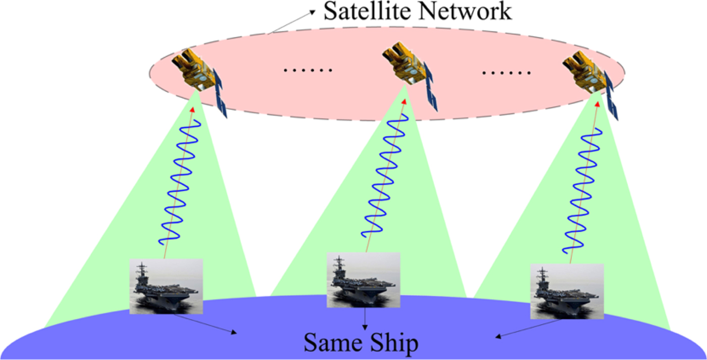
From public information, a few countries, such as the United States of America (USA) and Russia, currently have electronic intelligence satellites (Globalsecurity.org, 1993), and some commercial systems are planned to launch to perform high-precision geolocation of ships or other platforms (CaJacob et al., Reference CaJacob, McCarthy, O'Shea and McGwier2016). The USA has developed a third generation of electronic intelligence system for ocean surveillance as depicted in Figure 1, which can detect radars and other emitters from ships at sea and locate them to km-level positioning accuracy. Through a network consisting of multiple satellites, the surveillance system can monitor and track ships dozens of times per day.
Ocean surveillance system.

Emitter or passive tracking has been previously based mainly on various tracking frameworks, such as Joint Probabilistic Data Association (JPDA), Multiple Hypothesis Tracking (MHT) (Reid, Reference Reid1979; Blackman and Popoli, Reference Blackman and Popoli1999) and Random Finite Set (RFS) (Vo et al., Reference Vo, Vo and Cantoni2008). Among them, MHT is based on multi-frame data association, and it includes the whole process of tracking. MHT is more suitable for target tracking under high data association uncertainty although it is of greater computational complexity. JPDA and other single-frame tracking methods, which assume that the number of targets is fixed, can have errors once the number in the scene changes. RFS is a new theory used for tracking, mainly including Probability Hypothesis Density (PHD), Bernoulli filter, etc. These filters do not take into account data association between measurements and tracks, and only estimate the target state for a high computational efficiency, and need to add labels or further combine other methods to obtain targets' tracks. To make use of other information to improve tracking performance, there are many improved algorithms using the features of emitters, such as algorithms combining features with JPDA (Lei et al., Reference Lei, Tang and Gang2008) and PHD (Zhu and Zhou, Reference Zhu and Zhou2014). Due to the complex research background of electronic intelligence satellites, there is little relevant published research on ship tracking.
In our proposal for ship tracking with satellite electronic information, the main work includes multi-ship track estimation (the number of ships and their motion states) and multi-emitter state estimation (the number of emitters and their feature parameters) for each ship. In cases without prior knowledge of emitters, the process of tracking ships requires feature parameter estimation while tracking. The estimated parameters are used for further identification with multi-source information. However, the revisit time of the satellite network (usually an hour-level revisit interval) is long and unequal, and the emitter turns on randomly, making satellite electronic information discontinuous compared with an active detection system (second-level sampling rate). The low positioning accuracy and some clutter caused by environment noise and self-noise of passive location (Xia et al., Reference Xia, Zou, Lei and Zhu2014) have also increased the difficulty of tracking. Moreover, ships often carry multiple emitters: for example, an aircraft carrier is equipped with multiple radars working at different frequencies for air search, sea search, air traffic control, and target illumination. The above problems make it difficult to estimate the states of ships accurately by single-frame tracking methods, while MHT is preferred for this track application and the track performance can be ensured by multi-frame data association. An electronic intelligence satellite (usually in low orbit) can obtain multiple measurements of the same emitter over a short period by intercepting emitter signals, but it is hard to estimate the motion state using these measurements due to the slow movement of a ship and poor positioning accuracy. For example, the time of a satellite passing overhead of a ship is about 5 min with 3 km positioning error, and the speed of the ship is about 10 m/s. Ten positions of the ship are obtained, so the change of ship position is relatively small compared with the positioning error. Ignoring the short distance of ship movement during the time of a satellite overhead, we assume that all measurements of an emitter are obtained at the same time, and each emitter can be regarded as an extended target. There are several published approaches to solve the Extended Target Tracking (ETT) problem. The main methods include a Bayesian solution under different hypotheses (Koch, Reference Koch2008; Baum and Hanebeck, Reference Baum and Hanebeck2014), RFS (Granstrom et al., Reference Granstrom, Lundquist and Orguner2012; Granstrom and Orguner, Reference Granstrom and Orguner2012) and classical tracking methods with pre-processing (Vivone and Braca, Reference Vivone and Braca2016). Considering the characteristics of an emitter and the computational burden, we use pre-processing and a MHT to solve the ETT problem in this paper.
This paper is organised as follows. We introduce a standard MHT method in Section 2 and then discuss the modelling of a ship target based on the characteristics of satellite electronic information of emitters in Section 3. In Section 4, we propose an improved MHT method with feature information, which is the main contribution of our paper. In particular, the incorporation of feature information into the MHT framework is presented. Simulation results are discussed in Section 5, followed by a summary of the work and conclusions in Section 6.
2. MHT FRAMEWORK
MHT is a multiple target tracking algorithm, which has been widely used in many tracking applications. A key strategy in MHT is to use multi-frame measurements for data association, through delaying a decision by keeping multiple hypotheses to resolve data association ambiguities. MHT involves track initiation, track maintenance and track termination in a unified framework, which is more prominent in the case of low detection probability, large clutter density and dense targets. There are mainly two kinds of MHT frameworks (Blackman, Reference Blackman2004): Hypothesis-Oriented MHT (HOMHT) and Track-Oriented MHT (TOMHT). Because the TOMHT approach is preferred in tracking applications due to its efficiency (Ren et al., Reference Ren, Huang, Sun, Liu and Wu2014; Kim et al., Reference Kim, Li, Ciptadi and Rehg2015), this paper focuses on TOMHT and details of some elements of a typical TOMHT are described in this section.
2.1. Track tree formation
TOMHT uses the structure of track trees to manage targets. A track tree corresponds to a target, each node on the track tree corresponds to a measurement (including dummy measurements) and each path from the root node to the leaf node corresponds to a track hypothesis, of which only one track corresponds to the real track of the target. At each frame, a new track tree is constructed for each measurement to account for a new target. The previously existing track is extended by spawning a separate branch for each measurement within its gating area. If no measurements are associated with the track, an empty node is spawned.
2.2. Track score
The track score is used to evaluate each track in MHT, and it can be defined as the cumulative Log-Likelihood Ratio (LLR). According to Bayesian theory, the score of the j-th track at frame j can be expressed in the following recursive form,
 $$S^j(k)=S^j(k-1)+\Delta S^j(k)$$
where ΔS j(k) is the increment of the track score, which is calculated as
 $$\Delta S^j(k) = \left\{ {\matrix{ {\ln \left( {\displaystyle{{P_{\rm D}} \over {{(2\pi )}^{q/2}(\rho _{\rm n} + \rho _{\rm f})\sqrt { \vert \sum\limits_k^j \vert } }}} \right) - \displaystyle{{d_{\rm M}^2 } \over 2},} \hfill & {i > 0} \hfill \cr {\ln {\mkern 1mu} (1 - P_{\rm D}),} \hfill & {i = 0} \hfill \cr } } \right.$$
where P D is the probability of detection, ρn and ρf are the spatial density of new targets and clutter, respectively,  $\sum^{j}_{k}$ is the covariance matrix which is estimated by a Kalman filter for the j-th track at frame k, q is the state dimension and d M is the Mahalanobis distance between an observation location and a predicted location. i > 0 means the j-th track is associated with the i-th measurement at frame k while i = 0 means the j-th track is associated with the dummy measurement. Each measurement can initialise a new track, and the initial score of each track is S j(1) = ρ n/ρ f.
2.3. Global hypothesis formation and pruning
The global hypothesis formation is equivalent to the Multidimensional Assignment (MDA) or the Maximum Weight Independent Set (MWIS) problem (Papageorgiou and Salpukas, Reference Papageorgiou and Salpukas2009) and the MWIS problem is relatively easy to solve. An undirected graph G(V, B) is constructed by assigning each track to a graph vertex g j, g j ∈ V. A weight w j of the vertex g j corresponds to its track score S j(k). An edge (i, j) ∈ B connects two vertices g i and g j if the two tracks share common observations. An independent set is a set of vertices with no edges in common. Hence, finding MWIS is equivalent to finding the set of compatible tracks that maximises the total track score. This can be expressed as an integer linear programming problem,
 $$\eqalign{\max_{g_i} &\quad \sum_i g_iw_i \cr \hbox{s.t.}&\quad g_i+g_j\le 1,\ \forall(i,j)\in B\quad g_i\in \{0,1\},\ \forall i }$$
where s.t. is the abbreviation of “subject to”. Because of the exponential increase in the number of track hypotheses over time (Kim et al., Reference Kim, Li, Ciptadi and Rehg2015), it is necessary to apply some strategies to reduce computational complexity. There are many pruning mechanisms in a classical MHT implementation. In this paper, we use N-scan pruning and global pruning based on the posterior probability of each track. The N-scan pruning makes the data association decisions at frame k − N + 1 using old measurements from frame k − N + 1 to k. After N-scan pruning is completed, global track deletion is performed based on the track probability. All tracks with a probability lower than a threshold will be deleted. For more details about pruning mechanisms, see Blackman and Popoli (Reference Blackman and Popoli1999).
3. MODELLING OF TARGET
3.1. Motion model
Ships' tracks mainly include great-circle and rhumb-line navigation tracks (Sölver and Marcus, Reference Sölver and Marcus1958). The former is the shortest track, but in reality, piecewise rhumb-line tracks are normally used to approximate the great-circle track due to its frequent changes of course. Therefore, the latter is studied in this paper. Latitude and longitude are usually used to describe position and can be transformed into plane coordinates by projections, such as the Transverse Mercator (TM) projection and the Universal TM (UTM) projection. The revisit interval of an electronic intelligence satellite network is so long that the target state has a deformation in the projection plane, which affects the precision of prediction of the target state. Therefore, we describe the target state in geographical coordinates, that are defined in frame k as
 $${\bi x}_k=(\lambda_k, \dot{\lambda}_k, \varphi_k,\dot{\varphi}_k)^{\rm T}$$
where λk, φk and  $\dot{\lambda}_{k}$,
 $\dot{\varphi}_{k}$ represent the position and velocity components along longitude and latitude directions, respectively. The basic unit of latitude, longitude, and course is the degree (°). The units of distance, time and velocity are nautical miles (nm), hours (h), knots (kn, kn = nm/h), respectively. The locations in the northern and southern hemisphere are denoted as positive and negative latitudes, respectively, while locations in the eastern and western hemisphere are denoted as positive and negative longitudes, correspondingly. Given the speed v k and the course θk over ground (relative to true north), it can be obtained that
 $$\left\{ {\matrix{ {{\dot \lambda }_k = v_k\sin \theta _k} \cr {{\dot \varphi }_k = v_k\cos \theta _k} \cr } } \right.$$
Middle latitude sailing is simpler and more convenient to use in the dead reckoning of a rhumb-line track (Sölver and Marcus, Reference Sölver and Marcus1958), so we use it for track prediction. The state transition model from one point (λ1, φ1) to the other point (λ2,φ2) is
 $$\left\{ \matrix{\varphi _2 = \varphi _1 + \dot \varphi T/a \hfill \cr \lambda _2 = \lambda _1 + \dot \lambda T{\mkern 1mu} {\rm sec}(\varphi ^{\rm m})/a \hfill} \right.$$
where T is the time interval, a is the conversion factor which equals 60 nm/° since 1° of longitude along the equator is approximately 60 nm. φm is the middle latitude at which the arc length of the parallel separating the meridians passing through two specific points is exactly equal to the departure in proceeding from one point to the other. φm is approximately the mean latitude in sailing (Bowditch, Reference Bowditch2011),
 $$\varphi^{\rm m}=(\varphi_1+\varphi_2)/2=\varphi_1+\dot{\varphi}T/(2a)$$
As can be seen from Equation (6), λ2 is prone to larger errors at high latitudes than at low latitudes when the errors of φm are the same due to the secant function. λ2 tends to infinity when  $\varphi^{\rm m}=\pm90^{\circ}$, so Equation (6) cannot be used accurately in the high north or the far south. If we want to track ships at high latitudes (latitude higher than 80°), we should use other coordinate systems, such as universal polar stereographic coordinates which cover the Earth's polar regions (Hager et al., Reference Hager, Behensky and Drew1989). In this paper, the region in which we are interested is at low and middle latitudes. The motion model can be described as
 $${\bi x}_k=f_{k-1}({\bi x}_{k-1})+{\bi G}_{k-1}{\bi v}_{k-1}$$
where f k−1( · ) is the state transition function, and Gk−1 and vk−1 are the process noise matrix and process noise, respectively. We define  ${\bi v}_{k-1}=\lpar \ddot{\lambda}_{k-1}\comma \; \ddot{\varphi}_{k-1}\rpar ^{\rm T}$ and vk−1 represents a multivariate Gaussian with zero mean. The standard deviations of
 $\ddot{\lambda}_{k-1}$ and
 $\ddot{\varphi}_{k-1}$ are both set to σv. Derived from Equation (6), the state transition equation is
 $$\matrix{ {x_k} \hfill & { = \left[ {\matrix{ {\lambda _k} \cr {{\dot \lambda }_k} \cr {\varphi _k} \cr {{\dot \varphi }_k} \cr } } \right] = \left[ {\matrix{ {\lambda _{k - 1} + {\dot \lambda }_{k - 1}T_{k - 1}{\rm sec}(\varphi _{k - 1}^{\rm m} )/a} \cr {{\dot \lambda }_{k - 1}} \cr {\varphi _{k - 1} + {\dot \varphi }_{k - 1}T_{k - 1}/a} \cr {{\dot \varphi }_{k - 1}} \cr } } \right]} \hfill \cr {} \hfill & {\quad + \left[ {\matrix{ {{(T_{k - 1})}^2{\mkern 1mu} {\rm sec}(\varphi _{k - 1}^{\rm m} )/(2a)} & 0 \cr {T_{k - 1}} & 0 \cr 0 & {{(T_{k - 1})}^2/(2a)} \cr 0 & {T_{k - 1}} \cr } } \right]\left[ {\matrix{ {{\ddot \lambda }_{k - 1}} \cr {{\ddot \varphi }_{k - 1}} \cr } } \right]} \hfill \cr } $$
with T k−1 = t k − t k−1,  $\varphi^{\rm m}_{k-1}=\varphi_{k-1}+\dot{\varphi}_{k-1}T_{k-1}/\lpar 2a\rpar $, where t k−1 and
 $\varphi^{\rm m}_{k-1}$ are the time stamp and the middle latitude at frame k − 1, respectively.
3.2. Measurement model
By means of geolocation processing (multi-satellite time difference of arrival technique, etc.) in the short receiving time available, we can get the longitude and latitude of an emitter, which is used as the position measurement zk. The measurement equation for position information at frame k is
 $${\bi z}_k={\bi H}_k{\bi x}_k+{\bi w}_k,{\bi w}_k\sim N(\bf{0},{\bi R}_k)$$
 $${\bi H}_k = \left[ {\matrix{ 1 & 0 & 0 & 0 \cr 0 & 0 & 1 & 0 \cr } } \right]$$
 $${\bi R}_k = \left[ {\matrix{ {\sigma _\lambda ^2 } & 0 \cr 0 & {\sigma _\varphi ^2 } \cr } } \right]$$
where Hk is the observation matrix, wk is the position noise and Rk is the error covariance matrix which dominates the spread of measurements (spatial extension or shape). σ λ and σ φ are the standard deviations of positioning in longitude and latitude, respectively. Different circles of latitude have different lengths, and the Equator is the longest. To correspond to Equation (6), we set
 $$\sigma_\varphi=\sigma_{\rm p},\sigma_\lambda=\alpha\sigma_{\rm p},\alpha\ge 1$$
where σp is the standard deviation of positioning at the Equator, α is the weight in longitude and it should increase with an increase of latitude. To simplify processing, α is set to a constant in the surveillance region. Since an emitter is regarded as an extended target, we assume that the number of measurements from each emitter obtained by the satellite receiver is in a Poisson distribution.
An electronic intelligence satellite can not only acquire position information of emitters, but also obtain rich feature information such as Centre Frequency (CF), Pulse Repetition Interval (PRI) and Pulse Width (PW) by the processing of emitter signals. The CF is the carrier frequency of the electromagnetic wave and it is more able to reflect the characteristics of an emitter compared with other features.
Therefore, in order to simplify the feature model, only the CF of an emitter is used as the feature information in this paper. In reality, the CF often changes for anti-jamming and anti-reconnaissance, and the changes of CF of different emitters vary. For example, the CF range of a navigation radar is much smaller than that of an early-warning radar, and the frequency of some phased array radars can range over a few hundred Mega-Hertz (MHz). We assume that each ship is equipped with one or more emitters, and the CF of each emitter is a one-dimensional Gaussian distribution with different means and variances. As the measure accuracy of frequency is high (generally less than 1 MHz), the measurement error of the CF can be negligible compared with the frequency range. The measurement equation for frequency information is defined as follows,
 $$f_k=e^i_k,e^i_k\sim N(\mu_i,\sigma^2_i)$$
where f k denotes the frequency measurement,  $e^{i}_{k}$ is the true CF of the i-th emitter of a ship and μi and σi are the mean and the standard deviation of CF, respectively.
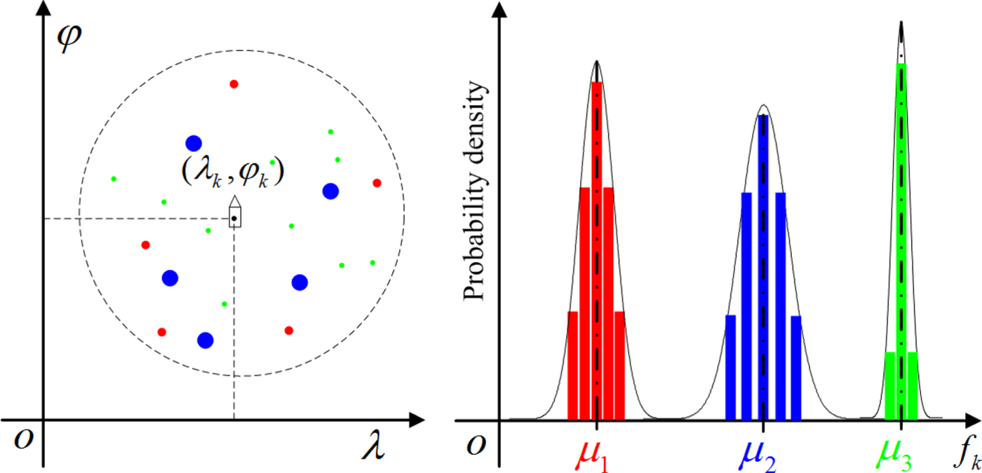
In this paper, both position information and feature information are used in a measurement and the augmented measurement is denoted as  $\tilde{{\bi z}}_{k}=\lcub {\bi z}_{k}\comma \; f_{k}\rcub $ when satellites revisit the target at frame k. As shown in Figure 2, by simulation, a ship is equipped with three emitters with different means and variances of CF, and each emitter can produce multiple measurements during the short time when a satellite passes over the ship. The positions of measurements (left part of Figure 2) are distributed around the ground truth position of the ship. Points in different colours represent the measurements of different emitters. The centre frequencies of measurements (right part of Figure 2) are distributed around different means.
A simulated example of measurement distribution of a ship.

4. JOINT KINEMATIC AND FEATURE TRACKING
4.1. Pre-processing of measurements
In a complex electromagnetic environment, an electronic intelligence satellite can not only receive emitter signals, but also receive clutter resulting in a large number of false positioning measurements. Measurements of an extended target cannot be directly used for tracking. Therefore, a pre-processing of measurements, which mainly includes two clustering operations, is performed to feed the tracking algorithm. The first clustering operation is to cluster the measurements of the same emitter to get a new measurement and reduce clutter, and the second operation is to cluster different emitters from the same ship, so as to track ships instead of tracking emitters and improve the accuracy of tracking.
To solve the clustering problem with the number of targets unknown, we use agglomerative hierarchical clustering (Jain et al., Reference Jain, Murty and Flynn1999) with the location and frequency information. The new measurements obtained after the first and the second clustering are represented as a dot and two dots on the top of measurements, respectively. The process is as follows:
(1) First clustering operation.
Input: Measurement set  $\tilde{{\bi Z}}_{k}=\lcub \tilde{{\bi z}}^{i}_{k}\comma \; 1\le i\le N_{k}\rcub $,
 $\tilde{{\bi z}}^{i}_{k}=\lcub {\bi z}^{i}_{k}\comma \; f^{i}_{k}\rcub $, where N k indicates the total number of measurements at the k-th revisit time.
Initialisation: Select each measurement as the initial cluster which is defined as  $W_{i}=\lcub \tilde{{\bi z}}^{i}_{k}\rcub $. The maximum distance between the clusters is used to measure similarity, that is
 $$d(W_i,W_j)=\max_{\tilde{{\bi z}}^m_k\in W_i,\tilde{{\bi z}}^n_k\in W_j} d(\tilde{{\bi z}}_k^m,\tilde{{\bi z}}_k^n)$$
The distance between two measurements is defined as
 $$d(\tilde{{\bi z}}_k^i ,\tilde{{\bi z}}_k^j ) = \left\{ {\matrix{ {\displaystyle{{ \vert f_k^i - f_k^j \vert } \over {\Delta f_k}},} \hfill & {{\rm if }d_{\rm M}({\bi z}_k^i ,{\bi z}_k^j ) \le \sqrt {\delta _{{\rm P}_{\rm G}}} } \hfill \cr {1,} \hfill & {{\rm otherwise}} \hfill \cr } } \right.$$
 $$d_{\rm M}({\bi z}_k^i ,{\bi z}_k^j ) = \sqrt {{({\bi z}_k^i - {\bi z}_k^j )}^T{\left[ {\matrix{ {2{(\sigma _{\rm p})}^2} & 0 \cr 0 & {2{(\alpha \sigma _{\rm p})}^2} \cr } } \right]}^{ - 1}({\bi z}_k^i - {\bi z}_k^j )} $$
where Δ f k is the range of frequency measurement at frame k,  $\Delta f_{k}=\max\limits_{i} f_{k}^{i}-\min\limits_{i} f_{k}^{i}$ and
 $d_{\rm M}\lpar {\bi z}_{k}^{i}\comma \; {\bi z}_{k}^{j}\rpar $ denotes the Mahalanobis distance between two measurements. Ignoring slow movement of ships during the time that satellites are overhead, d M2 is a χ2 distribution with two degrees of freedom.
 $\delta_{{\rm P}_{\rm G}}$ is a threshold which can be computed using inverse cumulative χ2 distribution for a given probability P G, where
 $\delta_{{\rm P}_{\rm G}}=\hbox{invchi}2\lpar P_{\rm G}\rpar $, and invchi2( · ) is the function of inverse cumulative χ2 distribution. If
 $\delta_{{\rm P}_{\rm G}}$ is small, measurements from the same emitter cannot be clustered, which would cause a lot of false targets. If
 $\delta_{{\rm P}_{\rm G}}$ is too large, measurements from different emitters (relatively close to each other with equal frequencies) may be clustered. However, the impact of wrong clustering caused by a large
 $\delta_{{\rm P}_{\rm G}}$ on tracking can be reduced by multi-frame data association. We set
 $\delta_{{\rm P}_{\rm G}}=8$ for
 $P_{G}\approx98\percnt $ to ensure measurements of the same emitter can belong to the same cluster and reduce false targets.
Loop: Find the nearest two clusters W m and W n, and merge them to obtain a new cluster W t,  $W_{t}=W_{m}\cup W_{n}$. When the distance between clusters is greater than a threshold f T, we stop clustering. Taking into account the frequency range of the same emitter, f T is set to 200/Δ f, which means frequency measurements within 200 MHz will be regarded as one cluster.
Output: Cluster set {W i, 1 ≤ i ≤ N m}, where N m is the number of clusters. Considering that more than one measurement of an emitter can be obtained, W i is saved when the number of measurements is greater than one, otherwise it is regarded as clutter to be removed. The new cluster set is defined as  $\lcub \dot{W}_{t}\comma \; 1\le i\le \dot{N}_{\rm m}\rcub $, where
 $\dot{N}_{\rm m}$ is the number of saved clusters. We define a new measurement set as
 $\dot{\tilde{{\bi Z}}}=\lcub \dot{\tilde{{\bi z}}}^{i}_{k}\comma \; 1\le i\le \dot{N}_{m}\rcub $, where
 $\dot{\tilde{{\bi Z}}}^{i}_{k}=\lcub \dot{{\bi z}}^{i}_{k}\comma \; F^{i}_{k}\rcub $,
 $F^{i}_{k}=\lsqb \mu^{i}_{k}\comma \; \sigma^{i}_{k}\comma \; L^{i}_{k}\rsqb $.
 $\dot{\tilde{{\bi Z}}}^{i}_{k}$ is the mean of position measurements in
 $\dot{W}_{i}$,
 $\mu^{i}_{k}$,
 $\sigma^{i}_{k}$ and
 $L^{i}_{k}\lpar L^{i}_{k}\ge 2\rpar $ are the mean, the standard deviation and the number of frequency measurements in
 $\dot{W}_{i}$, respectively. The standard deviations of positioning for a new position measurement
 $\dot{{\bi z}}^{i}_{k}$ in latitude and longitude are approximately
 $\sigma_{\rm p}/\sqrt{L^{i}_{k}}$ and
 $\alpha\sigma_{\rm p}/\sqrt{L^{i}_{k}}$, respectively.
(2) Second clustering operation.
According to the above clustering method, we merge measurements in  $\dot{\tilde{{\bi Z}}}_{k}$ if their Mahalanobis distance
 $d_{\rm M}\lpar \dot{{\bi z}}^{i}_{k}\comma \; \dot{{\bi z}}^{j}_{k}\rpar $ is below the threshold
 $\sqrt{\delta_{{\rm P}_{\rm G}}}$,
 $$d_{\rm M}({\dot{{\bi z}}^{i}_{k}},{\dot{{\bi z}}^{j}_{k}}) = \sqrt {{({\dot{{\bi z}}^{i}_{k}} - {\dot{{\bi z}}^{j}_{k}})}^{\rm T}{\left[ {\matrix{ {{(\sigma _{\rm p})}^2(1/L_k^i + 1/L_k^j )} & 0 \cr 0 & {{(\alpha \sigma _{\rm p})}^2(1/L_k^i + 1/L_k^j )} \cr } } \right]}^{ - 1}({\dot{{\bi z}}^{i}_{k}} - {\dot{{\bi z}}^{i}_{k}})} $$
We also define a new measurement set as  $\ddot{\tilde{{\bi Z}}}_{k}=\lcub \ddot{\tilde{{\bi z}}}^{i}_{k}\comma \; 1\le i\le \ddot{N}_{\rm m}\rcub $ after the second clustering operation, where
 $\ddot{\tilde{{\bi z}}}^{i}_{k}=\lcub \ddot{\tilde{{\bi z}}}^{i}_{k}\comma \; E^{i}_{k}\rcub $,
 $E^{i}_{k}=\lcub F^{i}_{n\lpar k\rpar }\vert 1\le n\le N^{i}\rcub $. N̈ m is the number of clusters,
 $\ddot{{\bi z}}^{i}_{k}$ is the mean of position measurements in the i-th cluster, and
 $E^{i}_{k}$ is the frequency parameter set which contains multiple frequency measurements
 $F^{i}_{k}$ and
 $N^{i}_{k}$ is the number of
 $F^{i}_{k}$. In this paper,
 $\ddot{\tilde{{\bi Z}}}_{k}$ is used as the measurement set feeding the tracking. To simplify processing for tracking, we take
 $\sigma_{\rm p}/\sqrt{2}$ (the maximum after the first and the second clustering) in latitude and
 $\alpha\sigma_{\rm p}/\sqrt{2}$ in longitude as the unified standard deviations of positioning for all new measurements in the form of Equation (13).
4.2. Track score combined with features
The frequency measurement and the frequency state can be both regarded as Gaussian distributions. To better describe the feature similarity between emitters, Jensen-Shannon Divergence (JSD) (Lin, Reference Lin1991) is used to measure the distance of two frequency distributions. Assuming two Gaussian distributions p 1(x) = N(x; m1, P1) and p 2(x) = N(x; m2, P2), the JSD distance between them is defined as
 $$JSD(p_1\ \vert p_2)=\displaystyle{{1}\over{2}}(KLD(p_1\ \vert p_3)+KLD(p_2\ \vert p_3)),p_3=\displaystyle{{p_1+p_2}\over{2}}$$
 $$KLD(p_1\ \vert p_3)=\displaystyle{{1}\over{2}}\{\ln(\hbox{det}({\bi P}_3)/\hbox{det}({\bi P}_1))+ \hbox{tr}({\bi P}_1{\bi P}_3^{-1})-\hbox{dim}({\bi x})+({\bi m}_1-{\bi m}_3)^{\rm T} {\bi P}_3^{-1}({\bi m}_1-{\bi m}_3)\}$$
 $$KLD(p_2\ \vert p_3)=\displaystyle{{1}\over{2}}\{\ln(\hbox{det}({\bi P}_3)/\hbox{det}({\bi P}_2))+ \hbox{tr}({\bi P}_2{\bi P}_3^{-1})-\hbox{dim}({\bi x})+({\bi m}_2-{\bi m}_3)^{\rm T} {\bi P}_3^{-1}({\bi m}_2-{\bi m}_3)\}$$
 $${\bi m}_3=\displaystyle{{{\bi m}_1+{\bi m}_2}\over{2}}$$
 $${\bi P}_3=\displaystyle{{{\bi P}_1+{\bi m}_1^T{\bi m}_1+{\bi P}_2+{\bi m}_2^T{\bi m}_2}\over{2}}-{\bi m}_3^T{\bi m}_3$$
where KLD is Kullback-Leibler Divergence (KLD) (Duchi, Reference Duchi2007) and dim(·) represents the dimensionality of features. We define  $\hat{E}^{j}_{k-1}$ as the frequency state of the j-th track at frame k − 1, and
 $E^{i}_{k}$ as the i-th frequency measurement at frame k,
 $$\hat{E}^j_{k-1}=\{\hat{F}^j_{m(k-1)} \vert 1\le m\le M^j\},\hat{F}^j_{m(k-1)}=[\hat{\mu}^j_{m(k-1)},\hat{\sigma}^j_{m(k-1)},I^j_{m(k-1)}]$$
 $$E^j_k=\{F^i_{n(k)} \vert 1\le n\le N^i\},F^i_{n(k)}=[\mu^i_{n(k)},\sigma^i_{n(k)},L^i_{n(k)}]$$
where M j and N i may not be equal. We define the distance between two sets as
 $$d(E^i_k,\hat{E}^j_{k-1})=\min_{1\le n\le N^i}\min_{1\le m\le M^j} JSD(N(x;\mu^i_{n(k)},(\sigma^i_{n(k)})^2)\ \vert\vert N(x;\hat{\mu}^j_{n(k-1)},(\hat{\sigma}^j_{n(k-1)})^2))$$
To convert the distance into likelihood, we use Fuzzy C-Means (FCM) clustering (Jain et al., Reference Jain, Murty and Flynn1999) to calculate the membership degree of feature information. This clustering algorithm, which assumes each sample can belong to multiple categories, is a soft partition method based on an optimal function. Providing that there are N s samples from N c categories given a weighted power b, the FCM clustering problem can be expressed as
 $$\eqalign{ \min &\quad \sum^{N_{\rm s}}_{i=1}\sum^{N_{\rm c}}_{j=1}(u_{ij})^b(d_{ij})^2 \cr \hbox{s.t.}&\quad u_{ij}\in [0,1], i=1,2,\ldots,N_{\rm s}\quad j=1,2,\ldots,N_{\rm c} \cr &\quad \sum^{N_{\rm c}}_{j=1}u_{ij}=1,\forall i\quad 0< \sum^{N_{\rm s}}_{i=1}u_{ij}< N_{\rm s},\forall j }$$
where u ij and d ij represent the membership degree and the distance between the i-th sample and the j-th category respectively. Using the Lagrange multiplier method, the fuzzy membership degree is given by
 $$u_{ij}=\displaystyle{{1}\over{\displaystyle\sum^{N_{\rm c}}_{k-1}\left(\displaystyle{{d_{ij}}\over{d_{ik}}}\right)^{\displaystyle{{2}\over{b-1}}}}}=\displaystyle{{(d^2_{ij})^{\displaystyle{{1}\over{1-b}}}}\over{\sum^{N_{\rm c}}_{k-1}\lpar d_{ij}^2\rpar ^{\displaystyle{{1}\over{1-b}}}}}$$
Through the above formula, we can obtain u ij between  $E^{i}_{k}$ and
 $\hat{E}^{j}_{k-1}$ within the gating area. Taking into account the measurement error, the error of the estimated position and the maximum distance, the gating distance between the current measurement position and estimated position at a previous time is set to satisfy the constraint,
 $$(\ddot{{\bi z}}^i_k-{\bi H}_{k-1}{\bi x}^j_{k-1})^T (\ddot{{\bi z}}_k^i-{\bi H}_{k-1}{\bi x}^j_{k-1})\le {\bi v}_{\rm max}{\bi T}_{k-1}/a+\sqrt{2}\alpha\sigma_{\rm p}$$
where vmax is the maximum speed. The increment of the i-th track's score with feature information can be defined as
 $$\Delta S^j(k) = \left\{ {\matrix{ {\omega \Delta S_{{\rm kin}}^j (k) + (1 - \omega )\Delta S_{{\rm fea}}^j (k),} \hfill & {i > 0} \hfill \cr {\ln (1 - P_{\rm D}),} \hfill & {i = 0} \hfill \cr } } \right.$$
where  $\Delta S^{j}_{\rm kin}\lpar k\rpar $ and
 $\Delta S^{j}_{\rm fea}\lpar k\rpar $ are the increments of the kinematic and feature scores at frame k respectively, ω is the weight of kinematic information and
 $\Delta S^{j}_{\rm kin}\lpar k\rpar $ is calculated by Equation (2).
 $$\Delta S^j_{\rm fea}(k)=\ln (u_{ij}/p_e)$$
where p e denotes the possibility of a measurement belonging to an extraneous (false or new) target.
4.3. Prediction and update
The prediction and update of the track information include kinematic and feature information. As the state transition equation is nonlinear, we use a first-order Extended Kalman Filter (EKF) to predict and update the motion state. For an EKF, it is important to calculate the state transition matrix Fk−1, which is a Jacobi matrix obtained by using a partial derivative of the state vector in Equation (9), and it is obtained as
 $${\bi F}_{k-1} = \left[ {\matrix{ 1 & {\displaystyle{{T_{k - 1}{\rm sec}(\varphi _{k - 1}^{\rm m} )} \over a}} & {\displaystyle{{{\dot \lambda }_{k - 1}T_{k - 1}\tan (\varphi _{k - 1}^{\rm m} )} \over {a\cos (\varphi _{k - 1}^{\rm m} )}}} & {\displaystyle{{{\dot \lambda }_{k - 1}{(T_{k - 1})}^2\tan (\varphi _{k - 1}^{\rm m} )} \over {2a^2\cos (\varphi _{k - 1}^{\rm m} )}}} \cr 0 & 1 & 0 & 0 \cr 0 & 0 & 1 & {T_{k - 1}/a} \cr 0 & 0 & 0 & 1 \cr } } \right]$$
The detailed process of prediction and update can refer to a standard EKF (Jazwinski, Reference Jazwinski2007), which is not described here. The frequency information of the track is updated but not predicted, and the update can be expressed as
 $$\hat{E}^j_k=J(\hat{E}^j_{k-1}, F^i_{n(k)})\cup F^i_{l(k)}$$
where  $F^{i}_{n\lpar k\rpar }$ and
 $F^{i}_{l\lpar k\rpar }$ represent the frequency measurement used for estimation of an existing frequency and a new frequency, respectively, that satisfy
 $$ \vert \hat{\mu}^j_{m(k-1)}-\mu^i_{n(k)} \vert < \Delta f_1\quad \hbox{and}\quad \vert \hat{\sigma}^j_{m(k-1)}-\sigma^i_{n(k)} \vert < \Delta\sigma_1$$
 $$ \vert \hat{\mu}^j_{m(k-1)}-\mu^i_{l(k)} \vert >\Delta f_2,\forall m$$
That means the frequency measurement within tolerances Δ f 1 and Δσ 1 is used to update, and it is added as a new frequency if there is a difference of frequency excess Δ f 2 compared with all frequency states. J(·) denotes that  $F^{i}_{n\lpar k\rpar }$ is used to update
 $\hat{E}^{j}_{k-1}$ and the update of frequency information of the m-th emitter of the j-th ship is
 $$\hat{\mu}^j_{m(k)}=\displaystyle{{I^j_{m(k-1)}\hat{\mu}^j_{m(k-1)}+L^i_{n(k)}\mu^i_{n(k)}}\over{I^j_{m(k-1)}+L^i_{n(k)}}}$$
 $$(\hat{\sigma}^j_{m(k)})^2=\displaystyle{{I^j_{m(k-1)}[(\hat{\mu}^j_{m(k-1)})^2+(\hat{\sigma}^j_{m(k-1)})^2]+ L^i_{n(k)}[(\mu^i_{n(k)})^2+(\sigma^i_{n(k)})^2]}\over{I^j_{m(k-1)}+L^i_{n(k)}}}-(\hat{\mu}^j_{m(k)})^2$$
 $$I^j_{m(k)}=I^j_{m(k-1)}+L^j_{n(k)}$$
We use a logic-based method to perform track extraction. Tracks are confirmed by M-of-N test (we use 3-of-4 test) and are terminated after K (we set K = 3) missed detections. The new frequency of target is confirmed and outputted after the times of update is not less than a certain number (we use two times) in the whole process of tracking.
5. EXPERIMENTS
In order to evaluate the performance of the proposed algorithm, the improved MHT method with frequency feature (N-scan pruning parameter is set to 5, 3 and 1 separately) and the standard MHT method without frequency feature (N-scan pruning parameter is set to 5) are compared. In this paper, we adopt an Optimal Sub-Pattern Assignment (OSPA) (Schuhmacher et al., Reference Schuhmacher, Vo and Vo2008) distance as a performance metric which takes account of both the errors of location and the number of targets. The OSPA distance of two sets is defined as
 $$\bar{d}^{(c)}_p(X,Y)=\left[\displaystyle{{1}\over{n}}\left(\min_{\pi\in \Pi_n}\sum^m_{i=1}d^{(c)}(x_1,y_{\pi(i)})^p+c^p(n-m)\right)\right]^{1/p}$$
if m ≤ n, otherwise  $\bar{d}_{p}^{\lpar c\rpar }\lpar X\comma \; Y\rpar =\bar{d}_{p}^{\lpar c\rpar }\lpar Y\comma \; X\rpar $, where X = {x 1, …, x m} and Y = {y 1, …, y n} are the set of true target positions and the set of target position estimates respectively and 1 ≤ p ≤ ∞, c > 0, Πn is the set of all possible permutations of {1, 2, …, n} and the truncated Euclidean distance is d (c)(x i, y π(i)) = min(c, d (c)(x i, y π(i))). The cut-off distance c and order parameter p of OSPA for evaluating motion states are set to c = 1, p = 2 throughout our experiments. Since the means and standard deviations of the CF are required for estimation in our algorithm, these parameters are also measured using the OSPA distance, and the OSPA distance is calculated by
 $\lsqb \hat{\mu}\comma \; \hat{\sigma}\rsqb $ obtained by the end of tracking. As the range of positions and that of frequencies are different, we set a different cut-off distance with c = 1, 000 (p is unchanged) for evaluating feature states. The simulation environment is given as follows.
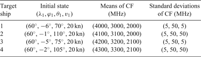
We suppose that there are four ships in the surveillance region during tracking and each ship is equipped with three emitters. The CF of each emitter is in a Gaussian distribution, and the detailed simulation parameters of targets are given in Table 1, where the unit of frequency is MHz. The measurements of each emitter of each ship are independent. The number of measurements of each emitter at each frame is assumed to follow a Poisson distribution with an expected number of 10, and the detection probabilities P D of each emitter are all set to 0.9. At each time, the clutter measurements are evenly distributed in the monitoring area, the number of clutter measurements is 400 and the frequencies of clutter are uniformly distributed in the range 1,000–5,000 MHz. The revisit time of the satellite constellation is set at unequal intervals, evenly distributed in the range of 0.5 ~ 2 h, and the number of overpasses is 40. The initial process noise standard deviation σv is set to 0.1 nm/h2. As the surveillance region is at low latitudes (near the equator), α is set to 1. The measurement noise standard deviation σp is set to 1/30°, approximately 3.7 km both in the x-axis and y-axis in Cartesian coordinates. The measurements are simulated by Equations (9)–(14). The main parameters used in our processing algorithm are set as: p e = 0.1, ω = 0.2, v max = 35 kn, Δf 1 = 50 MHz, Δσ 1 = 10 MHz, Δf 2 = 500 MHz. σ v = 0.1 nm/h2 and σ p = 1/30° in the EKF of MHT.
Parameters of four ships.

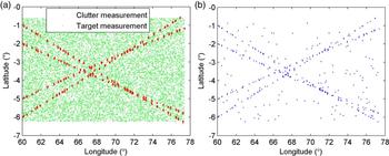
The measurement distribution generated by a simulation is shown in Figure 3(a), where target measurements and clutter measurements are mixed. Figure 3(b) shows the distribution of measurements after clustering twice. From the comparison before and after clustering, the effect of clustering combined with position and feature information is evident, as it can effectively reduce clutter and save valid measurements to improve the performance of the follow-up tracking algorithm.
Position distribution of measurements. (a) Input measurements. (b) Measurements after clustering.

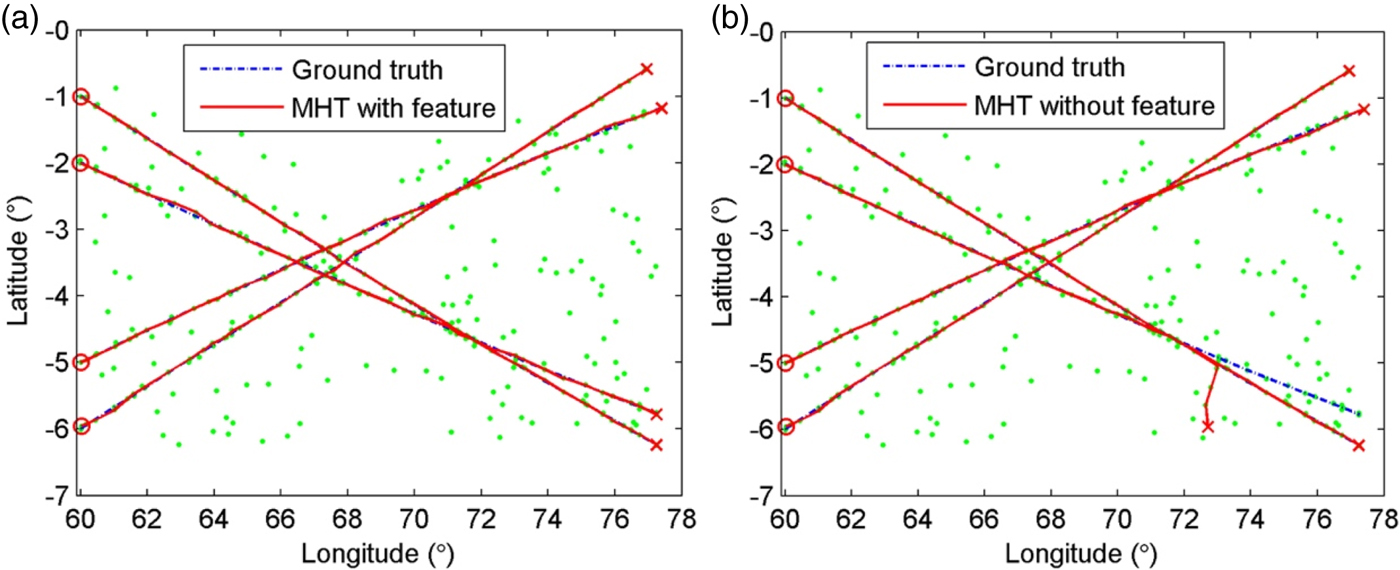
Figure 4 shows the tracking results of our algorithm and the standard MHT algorithm (Scan-5) under a simulation, where “o” represents the start of the track and “ + ” represents the end of the track. It can be seen that when the targets cross, track swap has occurred in the standard MHT algorithm, and there are some track fragmentations and false tracks, while the improved MHT algorithm can obtain the correct track with good stability of data association.
Tracking results of different algorithms. (a) MHT with feature. (b) MHT without feature.

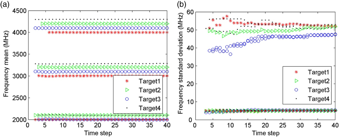
Figure 5 shows the estimation of means and standard deviations of CF under a simulation of the proposed algorithm. It can be seen that the algorithm can track while estimating parameters. This process can adaptively add the frequency information of emitters to realise an accurate estimation of frequency parameters in the case of random detection of each emitter. With the increase of tracking time, the frequency parameters gradually close to the ground truth.
Parameter estimation of frequency feature. (a) Means of CF. (b) Standard deviations of CF.

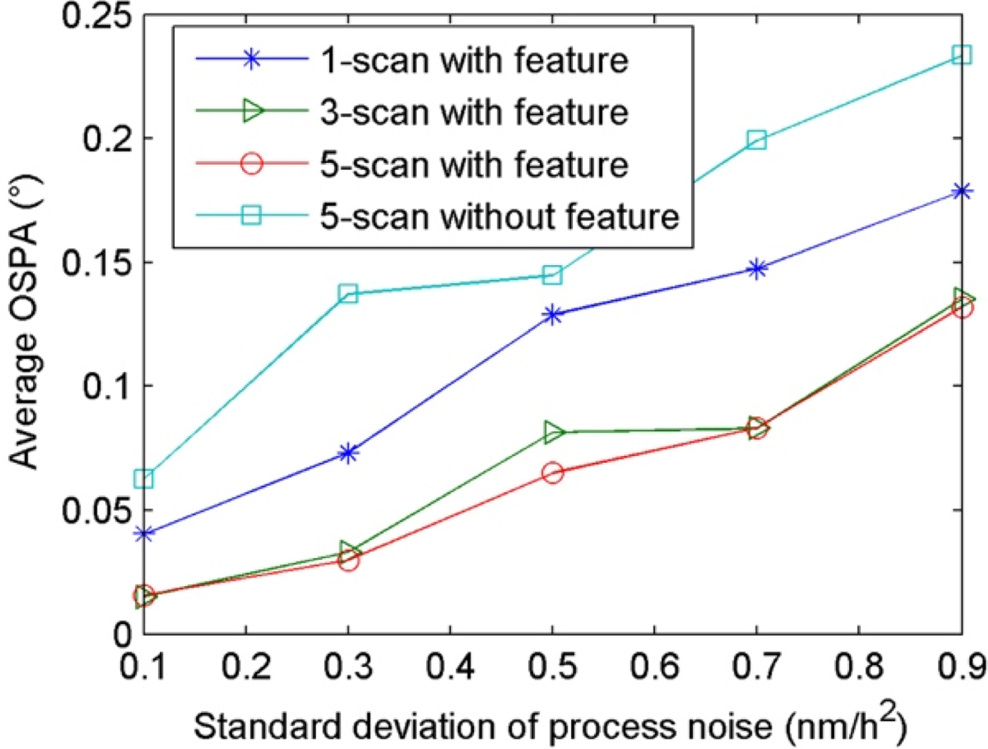
To verify the tracking performance of the proposed algorithm with a different uncertainty of the motion model, we compare the average OSPA (Monte Carlo experiments are repeated 100 times in each case) of two algorithms with different process noise standard deviations σv in a measurement simulation (other parameters are unchanged) as shown in Figure 6. Generally, for a greater σv, the more the uncertainty of movement will increase. It can be seen that the performance of MHT with the frequency feature is better than that of the standard MHT algorithm due to the feature incorporated into data association. In the standard MHT algorithm, the mismatch of process noise between filter and measurement reduces the accuracy of position estimation, causing track swap and track miss-association, thus increasing OSPA distance.
Tracking performance under different σv.

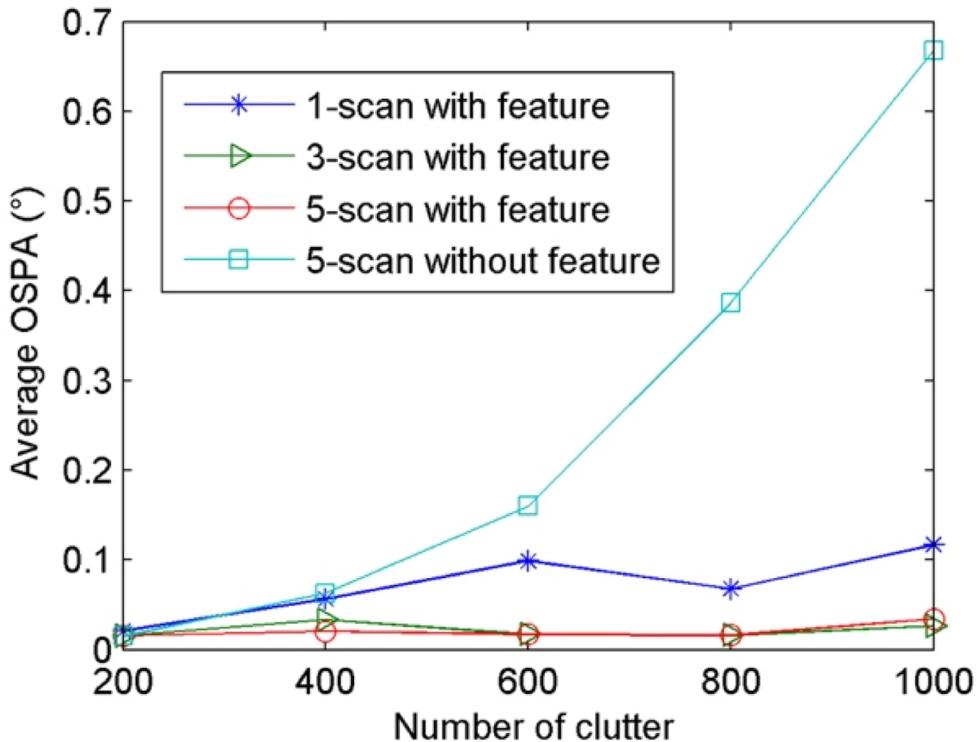
To validate the performance of our algorithm in the case of different clutter densities, the average OSPA distances (100 repetitions of Monte Carlo experiments) are compared under different amounts of clutter as shown in Figure 7. It can be seen that the performance of our algorithm using feature information is less sensitive to clutter, and can adapt to different clutter densities and estimate the target state accurately. This is mainly because most of the clutter is removed in pre-processing and the clutter is further reduced by using kinematic and feature information in data association. The tracking performance of MHT without frequency features drops sharply with the increasing amount of clutter due to false tracks caused by the wrong data association with clutter. The tracking performance of MHT with Scan-3 and Scan-5 are approximate, but they are better than the performance with Scan-1. This is because the multi-frame processing can resolve data association ambiguities effectively by keeping multiple hypotheses while MHT with Scan-1 is prone to produce false tracks even using features.
Tracking performance under different amounts of clutter.

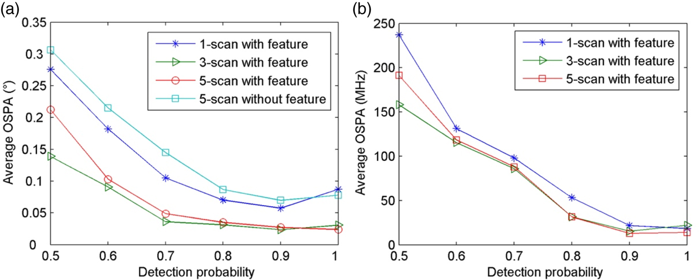
To further verify the tracking and parameter estimation performance of this algorithm in the scenario of multiple ships using multiple emitters with different detection probabilities, average OSPA distances are (100 repetitions of Monte Carlo experiments) compared under different P D for tracking and parameter estimation respectively, as shown in Figure 8. The lower the P D, the more randomness of detection will increase and the fewer measurements there will be. As can be seen from Figure 8(a), with the increase of P D, the performance of each algorithm increases. The performance of MHT with frequency features is better and results in an above 30% improvement in tracking. In Figure 8(b), we can see that with the increase of P D, the performance of parameters estimation is also improved, and the algorithm with multiple frames (Scan-5 and Scan-3) has higher parameter estimation performance than single-frame processing (Scan-1) in general, due to the higher tracking accuracy.
(a) Tracking performance under different P D. (b) Performance of parameter estimation under different P D.

Through the above experiments we can see that the performance of MHT with frequency features is better than that of MHT without frequency features, especially under clutter interference and randomness of detection. It also can be seen that the processing of multiple frames in MHT with frequency features is superior to single-frame processing. In view of the computation complexity, the processing of between three and five scans is suitable for most applications.
6. CONCLUSION
To achieve multi-ship track estimation and multi-emitter feature estimation using satellite electronic information, this paper proposes an improved tracking algorithm based on the MHT framework. The characteristics of this algorithm are as follows:
(1) The location and frequency information from emitters are used for clustering twice to partition measurements without prior knowledge, significantly reducing clutter and the complexity of data processing, improving the accuracy of tracking and the parameter estimation of targets.
(2) The track scores of frequency information based on JSD distance and FCM clustering are incorporated into the standard MHT framework, improving the accuracy and robustness of the data association.
(3) Tracks of multiple ships are generated based on prediction and update of motion states in geographical coordinates while an estimation of the emitter features is carried out, achieving a joint estimation of motion and feature states.
(4) The joint kinematic and feature tracking of ships has much better tracking performance than tracking using only kinematic information in the simulated scenarios. Meanwhile, the multi-frame data association in MHT can effectively improve the quality of data association and give better tracking accuracy than single-frame data association.
Satellite electronic information is obtained by passive location, so frequent silences of emitters will make detection probability low and tracking performance poor with track discontinuity and fragmentation. Therefore, in future work, we intend to study the fusion of multi-source information, especially the information from imaging satellites, to achieve better monitoring of ships.
FINANCIAL SUPPORT
This work was supported by National Natural Science Foundation of China under Grant No.91538201.