1. Introduction
The question of whether convergence exists between wealthy and impoverished nations stands as a central inquiry in the empirical growth literature (Barro and Sala-i-Martin, Reference Barro and Sala-i-Martin1992). This inquiry has spurred numerous studies investigating whether the income per capita, and more recently, labor productivity of poorer economies, is converging towards those of richer ones (Baumol, Reference Baumol1986; Barro and Sala-i-Martin, Reference Barro and Sala-i-Martin1992; Rodrik, Reference Rodrik2013). Among this extensive body of research, considerable attention is devoted to analyzing income and productivity convergence within the Eurozone. This focus is particularly intriguing as it offers insights into the productivity dynamics of economic integration and development within the Eurozone — a unique economic experiment wherein countries with diverse economic structures and levels of development share a common currency and monetary policy framework.
However, despite the abundance of research, evidence concerning convergence within the Eurozone remains inconclusive. For instance, Sondermann (Reference Sondermann2014) finds no evidence of convergence at the aggregate level but identifies signs of convergence for certain service sectors and manufacturing sub-industries. Similarly, Martino (Reference Martino2015) observes convergence in financial and business-related market services but not in manufacturing and aggregate productivity. In contrast, Rodrik (Reference Rodrik2013) provides a contrasting view, presenting evidence of strong unconditional convergence in manufacturing industries across over 100 countries, including those within the Eurozone.
This study aims to contribute to the existing literature by examining productivity convergence in manufacturing industries within the Eurozone from 1963 to 2018. To achieve this, we employ two related, innovative models: constant and varying-coefficient hierarchical panel data convergence regression models with two sets of latent factor structures—one set of global factors and another of industry-specific factors. Compared with conventional convergence regression models, these two models offer advantages in addressing three econometric issues largely overlooked in the convergence literature: (1) cross-sectional dependence, (2) parameter heterogeneity, and (3) data hierarchical structure (Durlauf et al. Reference Durlauf, Johnson, Temple, Durlauf, Johnson and Temple2005; Feng et al. Reference Feng, Gao and Peng2022).
Firstly, our hierarchical panel data models allow for cross-sectional dependence, a critical but often overlooked issue in the literature. Cross-sectional dependence refers to interdependencies among individual units due to common shocks, strategic interactions, or spillover effects. This issue has gained recent attention in panel data econometrics because neglecting it can lead to misleading inferences and inconsistent estimators (Andrews, Reference Andrews2005; Phillips and Sul, Reference Phillips and Sul2007). In the empirical growth literature, studies like Durlauf and Quah (Reference Durlauf, Quah, Durlauf and Quah1999) have shown that cross-sectional dependence significantly influences convergence dynamics. Pesaran (Reference Pesaran2004) also emphasizes the importance of accounting for cross-sectional dependence in growth regressions. Despite its significance, few studies in the cross-country convergence literature consider cross-sectional dependence.
In our study, cross-sectional dependence can occur at two levels: the total manufacturing level and the sub-manufacturing level. At the total manufacturing level, it impacts all manufacturing industries across all countries and can result from large-scale shocks like world oil price fluctuations and global financial crises. On the other hand, at the sub-manufacturing level, it affects specific subsets of industries and can stem from industry-specific events such as the implementation of Euro 6 standards, which primarily impact the automotive industry by necessitating investments in new emission-reducing technologies. Hence, it’s vital to consider cross-sectional dependencies at both levels. To address this, we incorporate two sets of latent factor structures into our convergence regression: one for global factors capturing dependencies at the total manufacturing level, and the other for industry-specific factors capturing dependencies at the sub-manufacturing level.
Secondly, our varying-coefficient hierarchical panel data model addresses parameter heterogeneity across industries, an issue often overlooked in the cross-country convergence literature. Many empirical studies in this field, as well as the broader empirical growth literature, assume uniform coefficients of convergence regressions across countries or industries. While this assumption aligns with new classical growth models, emerging research (e.g., Durlauf and Johnson, Reference Durlauf and Johnson1995; Durlauf et al. Reference Durlauf, Kourtellos and Minkin2001; Salimans, Reference Salimans2012) suggests heterogeneity in these coefficients. For example, Durlauf and Johnson (Reference Durlauf and Johnson1995) employ regression tree analysis to unveil distinct regimes in cross-sectional regression, indicating varied aggregate production functions among countries based on their development levels. Similarly, Durlauf et al. (Reference Durlauf, Johnson, Temple, Durlauf, Johnson and Temple2005) reveal compelling evidence of parameter heterogeneity across countries using a varying coefficient growth model.
In our study, we accommodate parameter heterogeneity by allowing convergence regression coefficients to vary across sub-manufacturing industries. This aspect of the model, coupled with the utilization of industry-specific factor structures, empowers us to investigate convergence dynamics not only at the aggregate manufacturing level but also at the sub-manufacturing industry level—a dimension scarcely explored in existing literature.
Thirdly, our hierarchical panel data models capitalize on the hierarchical structure inherent in industry-level data. In the empirical growth literature, the predominant use of country-level data often limits the depth of analysis and may overlook variations across different industries. By leveraging industry-level data, our study can exploit this nested structure to capture heterogeneity more effectively and offer nuanced insights into productivity dynamics. This approach is in line with recommendations from leading scholars. For instance, Hsiao (Reference Hsiao2014) underscores the advantages of hierarchical modeling in econometric analysis, emphasizing its capacity to accommodate nested data structures and capture within-group variations. Similarly, Gelman and Hill (Reference Gelman and Hill2007) advocate for hierarchical modeling techniques to handle hierarchical data structures and enhance parameter estimation precision. Through the integration of industry-level data and the adoption of a nested structure, our study aims to bolster the robustness and validity of its findings by more comprehensively elucidating the intricacies of productivity dynamics in the manufacturing industries with the Eurozone.
We apply the aforementioned models to a dataset encompassing 23 manufacturing industries across the 20 Eurozone countries over the period from 1963 to 2018. Our findings reveal both conditional and unconditional convergence within the manufacturing industry as a whole, as well as among the majority of the 23 sub-manufacturing industries at the ISIC two-digit level. Additionally, we observe notable disparities in convergence dynamics across sub-manufacturing industries. Furthermore, our robustness check, conducted using different subperiods, corroborates these findings. Finally, we compare the results of our model with those from two alternative models, further validating our conclusions.
The remainder of the paper is organized as follows: Section 2 introduces the hierarchical panel data convergence regression models. Section 3 outlines the estimation method employed for these models. Section 4 provides a brief description of the dataset used. Section 5 presents and discusses the empirical results. Section 6 compares these findings with those from alternative models. Finally, Section 7 concludes the paper.
2. The three-dimensional hierarchical panel data convergence regression model
In this section, we introduce the three-dimensional hierarchical panel data convergence regression model. We start by presenting the conventional two-dimensional country-level productivity convergence regression in Section 2.1. Then, we demonstrate the extension of this conventional model to derive the three-dimensional hierarchical panel data convergence regression model by incorporating cross-sectional dependence in Section 2.2 and parameter heterogeneity in Section 2.3. In Section 2.4, we highlight the novelty of our three-dimensional hierarchical panel data framework by comparing it with two notable recent studies.
2.1 The conventional two-dimensional productivity convergence regression
Most conventional convergence studies employ “cross-country growth regressions” using country-level data over a specified period. These regressions involve regressing the average growth rates of per capita income (or productivity) over an extended period against the initial level of income per capita (or productivity), along with additional control variables. A negative and significant coefficient on the initial labor productivity (or income per capita) is interpreted as evidence supporting
 $\beta$
-convergence. As highlighted by Durlauf (Reference Durlauf2003), “While
 $\beta$
-convergence is not the only statistical measure of convergence that has been developed, it is the dominant measure.”
Specifically, the conventional two-dimensional country-level productivity convergence regression is written as
 \begin{equation} y_{jt} = \mathbf {x}'_{jt} \boldsymbol {\beta }_0 + \epsilon _{jt}, \end{equation}
where
 $ j = 1, 2, \ldots , N$
indexes countries;
 $ t = 1, 2, \ldots , T$
indexes time;
 $ y_{jt}$
represents the rate of growth in labor productivity;
 $ \mathbf {x}_{jt}$
represents a set of observable explanatory variables including initial labor productivity and others suggested by Solow as well as other growth models, and
 $ \boldsymbol {\beta }_0$
denotes a coefficient vector associated with
 $ \mathbf {x}_{jt}$
; and
 $ \epsilon _{jt}$
represents an error term. This framework provides the foundation for examining productivity convergence by linking initial productivity levels and explanatory variables to subsequent growth rates. Equation (1) represents conditional convergence. Unconditional convergence is similar to Equation (1) but omits the control variables, resulting in a specification where initial productivity is the only explanatory variable. This allows for testing whether productivity disparities diminish over time purely through economic growth mechanisms, without accounting for structural or policy differences.
However, as outlined in the Introduction, the conventional country-level convergence regression model (1) faces three significant econometric challenges. Firstly, it assumes no cross-sectional dependence across countries and industries. Secondly, it fails to effectively utilize the hierarchical structure of industry-level data. Thirdly, it assumes that the parameters (i.e.,
 $\boldsymbol {\beta }_0$
) are homogeneous across all industries. To address these challenges, we extend the conventional cross-country convergence regression model in three ways: In Subsection 2.2, we incorporate cross-sectional dependence into the model through two sets of latent factor structures — one comprising global factors and the other industry-specific factors. In Subsection 2.3, we introduce parameter heterogeneity into the model by allowing its coefficients to vary across industries. Additionally, in both of these two sections we extend the two-dimensional conventional convergence regression model into a three-dimensional (country, industry, and time) hierarchical panel data convergence regression model, thereby enabling us to better utilize the hierarchical structure of industry-level data.
2.2 Dependence
We incorporate cross-sectional dependence into the conventional convergence regression in (1) by introducing two sets of unobservable factors: a set of global factors
 $(\boldsymbol {\gamma }^{G\prime }_{ij} \mathbf {f}^{\,G}_{t})$
and a set of industry-specific factors
 $(\boldsymbol {\gamma }^{S\prime }_{ij} \mathbf {f}^{\,S}_{it})$
:
 \begin{equation} y_{ijt} = \mathbf {x}'_{ijt} \boldsymbol {\beta }_{0} + \boldsymbol {\gamma }^{G\prime }_{ij} \mathbf {f}^{\,G}_{t} + \boldsymbol {\gamma }^{S\prime }_{ij} \mathbf {f}^{\,S}_{it} + \epsilon _{ijt}. \end{equation}
where
 $i = 1, 2, \ldots , L$
indexes industries and
 $j = 1, 2, \ldots , N_{i}$
.
 $\mathbf {f}^{\,G}_{t}$
represents a set of global factors that that affect all industries while
 $\boldsymbol {\gamma }^{G}_{ij}$
represents their associated loadings. Similarly,
 $\mathbf {f}^{\,S}_{it}$
represents a set of industry-specific factors that affect a subset of industries while
 $\boldsymbol {\gamma }^{S}_{ij}$
represents their associated loadings.
It is noteworthy that our hierarchical factor structure is quite general, encompassing several widely-used fixed effects as special cases. For example, when
 $\boldsymbol {\gamma }^{G}_{ij} = (\alpha _i + \gamma _j, 1)'$
and
 $\mathbf {f}^{\,G}_{t} = (1, g_{t})'$
, it reduces to the three-way fixed effects used in Abowd et al. (Reference Abowd, Kramarz and Margolis1999). Similarly, when
 $\gamma ^{G}_{ij} = D_{j}$
,
 $f^{G}_{t} = 1$
,
 $\gamma ^{S}_{ij} = 1$
and
 $f^{S}_{it} = D_{it}$
, our hierarchical factor structure reduces to the fixed effects employed in Rodrik (Reference Rodrik2013).
2.3 Parameter heterogeneity
We incorporate parameter heterogeneity by allowing the coefficients (i.e.,
 $\boldsymbol {\beta }_0$
) in (1) to vary across different sub-manufacturing industries, leading to the following modified version of the hierarchical panel data convergence regression model:
 \begin{equation} y_{ijt} = \mathbf {x}'_{ijt} \boldsymbol {\beta }_{i} + \boldsymbol {\gamma }^{G\prime }_{ij} \mathbf {f}^{\,G}_{t} + \boldsymbol {\gamma }^{S\prime }_{ij} \mathbf {f}^{\,S}_{it} + \epsilon _{ijt}. \end{equation}
From an economic perspective, equation (3) allows each sub-manufacturing industry to follow a different convergence process. From an econometric perspective, allowing the coefficients to vary across different industries in the hierarchical panel data convergence regression model facilitates consistent estimations of each industry-specific parameter vector,
 $\boldsymbol {\beta }_{i}$
. This is because it recognizes the inherent heterogeneity among industries, thereby improving the model’s accuracy and robustness.
It should be noted that we will estimate both versions of the hierarchical panel data convergence regression model (i.e., equation (2) and equation (3)). To distinguish between these two versions, in what follows we will refer to the one in (2) as the constant-coefficient hierarchical panel data convergence regression model while referring to the one in (3) as the varying-coefficient hierarchical panel data convergence regression model.
2.4 A novel hierarchical panel data framework
This section highlights the novelty of our three-dimensional hierarchical panel data framework by comparing it with two notable recent studies, Sun et al. (Reference Sun, Lin and Li2024) and Henderson and Soberon (Reference Henderson and Soberon2024), focusing on their research focus and approaches to addressing two critical issues in hierarchical panel data models: cross-sectional dependence and parameter heterogeneity.
First, we compare the research focus of the three studies, as their differing objectives result in distinct approaches to addressing cross-sectional dependence and parameter heterogeneity. Our framework introduces a three-dimensional parametric hierarchical panel data model specifically designed to analyze productivity convergence across the Eurozone’s manufacturing industries. In contrast, Sun et al. (Reference Sun, Lin and Li2024) extend earlier work on two-dimensional nonparametric panel data models with random effects to a three-dimensional framework, introducing two estimators for their proposed model. Similarly, Henderson and Soberon (Reference Henderson and Soberon2024) focus on summarizing and advancing the literature on three-dimensional nonparametric and semiparametric panel data models with fixed effects.
Second, we evaluate the distinct approaches of the three studies in addressing cross-sectional dependence. Because their research primarily targets other objectives, neither Sun et al. (Reference Sun, Lin and Li2024) nor Henderson and Soberon (Reference Henderson and Soberon2024) adequately address strong cross-sectional dependence arising from global shocks affecting all industries across countries or industry-specific shocks impacting subsets of industries. This limitation makes their models unsuitable for analyzing productivity convergence across the Eurozone’s manufacturing industries.
Specifically, Sun et al. (Reference Sun, Lin and Li2024) assume that errors in their model exhibit weak cross-sectional and temporal dependence, decomposing the error term into three pairwise random effects—individual-group-specific, individual-time-specific, and group-time-specific effects—along with an i.i.d. error term. While this approach effectively captures simple cross-sectional dependence, it assumes uncorrelated random components and does not allow for interactions across hierarchical levels. As a result, it cannot simultaneously model global shocks that affect all levels and industry-specific shocks that operate within subgroups. For example, while it captures dependencies within specific levels (e.g., individual-time or group-time effects), it fails to represent nested relationships, limiting its ability to capture the interplay between macroeconomic and sectoral forces.
Henderson and Soberon (Reference Henderson and Soberon2024), on the other hand, employ a fixed effects specification to address unobserved heterogeneity by removing means along various dimensions (e.g., individuals, time, and groups). Although this method is effective in eliminating simple forms of dependence, it assumes that dependencies can be fully captured by demeaning observed variables. This assumption limits its ability to model interactions across hierarchical levels. For instance, it cannot simultaneously account for global shocks (e.g., financial crises) and sector-specific shocks (e.g., regulatory changes), resulting in an incomplete representation of cross-sectional relationships.
In contrast, our proposed hierarchical panel data framework explicitly models nested dependencies, effectively capturing both broad macroeconomic influences and sector-specific shocks. By overcoming the limitations of Sun et al. (Reference Sun, Lin and Li2024) and Henderson and Soberon (Reference Henderson and Soberon2024), our framework offers a more accurate and comprehensive understanding of cross-sectional dependence among sub-manufacturing industries in the Eurozone, providing deeper insights into the dynamics of productivity convergence within these industries.
Third, we compare the approaches of the three studies in addressing parameter heterogeneity. Since their analyses are tailored to other research objectives, neither Sun et al. (Reference Sun, Lin and Li2024) nor Henderson and Soberon (Reference Henderson and Soberon2024) consider parameter heterogeneity arising from technological differences across sub-manufacturing industries. As a result, both studies assume homogeneity of coefficients across dimensions, making their models unsuitable for analyzing productivity convergence in the Eurozone’s manufacturing industries.
In contrast, our varying-coefficient hierarchical panel data model explicitly incorporates parameter heterogeneity. This flexibility enables the model to capture distinct convergence processes across industries, recognizing that each sub-manufacturing sector may follow its own trajectory due to structural or technological differences. For example, the convergence dynamics in labor-intensive industries, such as textiles, may differ significantly from those in capital-intensive industries, such as machinery and equipment. By allowing coefficients to vary across sub-industries, our framework provides deeper insights into the heterogeneity of productivity growth and convergence rates.
3. Estimation of the slope coefficients and the factor structure
In this section, we present the estimation of both the constant- and varying -coefficient hierarchical panel data convergence regression models in equations (2) and (3) respectively, as well as the factor structure.
We start by estimating the constant-coefficient hierarchical panel data convergence regression model in (2), which can be rewritten in vector form as follows:
 \begin{equation} \mathbf {Y}_{ij} = \mathbf {X}_{ij} \boldsymbol {\beta }_{0} + \mathbf {F}^{\,G} \boldsymbol {\gamma }^{G}_{ij} + \mathbf {F}^{\,S}_{i} \boldsymbol {\gamma }^{S}_{ij} + \mathbf {E}_{ij}, \end{equation}
where
 $\mathbf {E}_{ij} = (\epsilon _{ij1}, \ldots , \epsilon _{ijT})'$
;
 $\mathbf {Y}_{ij}$
and
 $\mathbf {X}_{ij}$
are defined in a similar manner.
 $\mathbf {F}^{\,G} = (\mathbf {f}^{\,G}_{1}, \ldots , \mathbf {f}^{\,G}_{T})'$
and
 $\mathbf {F}^{\,S}_{i} = (\mathbf {f}^{\,S}_{i1}, \ldots , \mathbf {f}^{\,S}_{iT})'$
. To estimate
 $\boldsymbol {\beta }_{0}$
and
 $\mathbf {F}=(\mathbf {F}_1,\ldots , \mathbf {F}_{i},\ldots ,\mathbf {F}_L)$
, where
 $\mathbf {F}_{i}=(\mathbf {F}^{\,G},\mathbf {F}^{\,S}_{i})$
, we firstly apply the following weighted least square method:
 \begin{equation} (\hat {\boldsymbol {\beta }}, \hat {\mathbf {F}}) = \textrm {argmin} Q(\boldsymbol {\beta }, \mathbf {F}), \end{equation}
where we have abused notation slightly on F for notational simplicity,
 \begin{equation} Q(\boldsymbol {\beta }, \mathbf {F}) = \sum _{i=1}^{L} \sum _{j=1}^{N_{i}} (\mathbf {Y}_{ij} - \mathbf {X}_{ij} \boldsymbol {\beta })' \mathbf {M}_{\mathbf {F}_i} (\mathbf {Y}_{ij} - \mathbf {X}_{ij} \boldsymbol {\beta }), \end{equation}
where
 $\mathbf {M}_{\mathbf {F}_i}$
is the orthogonal projection matrix obtained from
 $\mathbf {F}_i$
, such that
 $\mathbf {F}_i'\mathbf {F}_i/T=\mathbf {I}_{d_{\max }}$
, and
 $d_{\max } \, (\ge l^G+\max _i l_i^S)$
is a user specified large positive constant. Here, we require
 $T$
and
 $\min _{i}$
 $N_{i}$
to diverge in order to ensure consistent estimation, a requirement that becomes particularly evident when estimating each
 $\boldsymbol {\beta }_{i}$
. The strategy has been well adopted in the literature since Bai and Ng (Reference Bai and Ng2002). Obviously, (6) implies
 \begin{equation} \hat {\boldsymbol {\beta }} = \left ( \sum _{i=1}^{L} \sum _{j=1}^{N_{i}} \mathbf {X}_{ij}' \mathbf {M}_{\hat {\mathbf {F}}_i} \mathbf {X}_{ij} \right )^{-1} \sum _{i=1}^{L} \sum _{j=1}^{N_{i}} \mathbf {X}_{ij}' \mathbf {M}_{\hat {\mathbf {F}}_i} \mathbf {Y}_{ij}, \end{equation}
and, for
 $\forall i$
,
 $\hat {\mathbf {F}}_{i}$
is obtained via the following PCA (Principal Component Analysis) operation:
 \begin{equation*} \hat {\mathbf {F}}_{i} \hat {\mathbf {V}}_{i} = \hat {\boldsymbol {\Sigma }}_{i} \hat {\mathbf {F}}_{i}, \end{equation*}
where
 $\hat {\mathbf {V}}_{i} = \mathrm {diag}(\hat {\lambda }_{i,1}, \ldots , \hat {\lambda }_{i,d_{\max }})$
with
 $\hat {\lambda }_{i,1}, \ldots , \hat {\lambda }_{i,d_{\max }}$
being the largest
 $d_{\max }$
eigenvalues of
 $\hat {\boldsymbol {\Sigma }}_{i} = \sum _{j=1}^{N_{i}} (\mathbf {Y}_{ij} - \mathbf {X}_{ij} \hat {\boldsymbol {\beta }}) (\mathbf {Y}_{ij} - \mathbf {X}_{ij} \hat {\boldsymbol {\beta }})'$
.
Secondly, we turn to estimating the numbers of factors (
 $l^{G}$
and
 $l^{S}_{i}$
’s). The global factors affect all industries across all countries, while the industry-specific factors impact only a subset of industries. This distinction is crucial from a signal-to-noise ratio perspective, making it advantageous to ascertain the number of global factors initially. As outlined by Feng et al. (Reference Feng, Gao and Peng2022),
 $l^{G}$
and
 $l^{S}_{i}$
can be estimated respectively as follows:
 \begin{equation} \hat {l}^{G} = \textrm {argmin}_{l \leq d_{\max }} \left \{ \frac {\hat {\lambda }_{G,l+1}}{\hat {\lambda }_{G,l}} \cdot I(\hat {\lambda }_{G,l} \geq \omega ) + I(\hat {\lambda }_{G,l} \lt \omega ) \right \}, \end{equation}
and
 \begin{equation} \hat {\boldsymbol {\ell }}^{S} = \textrm {argmin}_{\boldsymbol {\ell }^{S}} \sum _{i=1}^{L} \left \{ \frac {\hat {\lambda }_{i,l_{i}^{S}+1}}{\hat {\lambda }_{i,l_{i}^{S}}} \cdot I(\hat {\lambda }_{i,l_{i}^{S}} \geq \omega ) + I(\hat {\lambda }_{i,l_{i}^{S}} \lt \omega ) \right \} , \end{equation}
where
 $\omega = 1/\log (T)$
,
 $\hat {\lambda }_{G,l} = 1$
is a mock eigenvalue,
 $\hat {\lambda }_{G,l}$
stands for the
 $l$
th largest eigenvalue of
 $\hat {\boldsymbol \Sigma }_{G} = \sum _{i=1}^{L} \hat {\boldsymbol {\Sigma }}_{i}$
,
 $\boldsymbol {\ell }^{S} = (l^{S}_{1}, \ldots , l^{S}_{L})$
with
 $0 \leq l^{S}_{i} \leq d_{\max }$
for
 $i \in [L]$
,
 $\hat {\lambda }^{S}_{i, 0} = 1$
is a mock eigenvalue, and
 $\hat {\lambda }^{S}_{i,l_{i}^{S}}$
stands for the
 $l_{i}^{S}$
th largest eigenvalue of
 $\hat {\boldsymbol \Sigma }^{S}_{i} = \mathbf {M}_{\hat {\mathbf {F}}_{G}}\hat {\boldsymbol {\Sigma }}_{i} \mathbf {M}_{\hat {\mathbf {F}}_{G}}$
with
 $\hat {\mathbf F}_{G}$
being the eigenfactors associated with the
 $\hat {l}^{G}$
largest eigenvalues of
 $\hat {\boldsymbol \Sigma }_{G}$
.
Finally, with
 $\hat {l}^{G}$
and
 $\hat {\boldsymbol {\ell }}^{S}$
in hand, we redo (5) to update our estimate of
 $\boldsymbol {\beta }_0$
. The estimation techniques described in equations (8) and (9) build upon frameworks introduced by Lam and Yao (Reference Lam and Yao2012) and Ahn and Horenstein (Reference Ahn and Horenstein2013). However, Lam and Yao (Reference Lam and Yao2012) emphasize an unresolved challenge in bounding the ratio of eigenvalues that approach zero from below. To address this issue, we introduce a tuning parameter, denoted as
 $\omega$
, which allows us to circumvent the difficulties associated with ratios whose denominators converge to zero. By incorporating an indicator function into equations (8) and (9), we construct a U-shaped curve, thus avoiding the need to directly address the problematic ratio. After fully recovering the factor structure, we can construct the confidence interval for
 $\boldsymbol {\beta }_0$
following the methodology outlined in Theorem 4 of Bai (Reference Bai2009).
With regard to the varying-coefficient hierarchical panel data convergence regression model in (3), a consistent estimator for each
 $\boldsymbol {\beta }_{i}$
can be established as in either Pesaran (Reference Pesaran2006) or Bai (Reference Bai2009), depending on the restrictions imposed on the regressors. For example, in Kapetanios et al. (Reference Kapetanios, Pesaran and Yamagata2021), the Common Correlated Effects approach of Pesaran (Reference Pesaran2006) is adopted by assuming that the regressors follow a factor structure. Once each
 $\boldsymbol {\beta }_{i}$
is consistently estimated (denoted by
 $\hat {\boldsymbol {\beta }}_{i}$
), one can estimate the global factors and the industry-specific factors by slightly modifying equations (8) and (9) as follows:
 \begin{eqnarray} &&\hat {\boldsymbol \Sigma }_{G} = \sum _{i=1}^{L} \sum _{j=1}^{N_{i}} (\mathbf {Y}_{ij} - \mathbf {X}_{ij} \hat {\boldsymbol {\beta }}_{i}) (\mathbf {Y}_{ij} - \mathbf {X}_{ij} \hat {\boldsymbol {\beta }}_{i})', \end{eqnarray}
 \begin{eqnarray} && \hat {\boldsymbol \Sigma }^{S}_{i} = \mathbf {M}_{\hat {\mathbf F}_{G}} \sum _{j=1}^{N_{i}} (\mathbf {Y}_{ij} - \mathbf {X}_{ij} \hat {\boldsymbol {\beta }}_{i}) (\mathbf {Y}_{ij} - \mathbf {X}_{ij} \hat {\boldsymbol {\beta }}_{i})' \mathbf {M}_{\hat {\mathbf F}_{G}}. \end{eqnarray}
4. Data
For labor productivity (or real value added per employee), we adopt the methodology outlined by Rodrik (Reference Rodrik2013), utilizing UNIDO’s INDSTAT2 database, which furnishes statistics for 23 manufacturing industries at the ISIC two-digit levelFootnote 1 across numerous countries. INDSTAT2 encompasses data on value added (in nominal U.S. dollars) and employment, among other indicators. Real value added is derived by deflating nominal value added using the U.S. producer price index. Subsequently, labor productivity is calculated by dividing real value added by employment (or the number of employees). The growth in labor productivity is then quantified as the percentage change in labor productivity.
Our variable of interest is the initial labor productivity, while our control variables include a broad spectrum of factors that have been deemed significant in assessing convergence. These factors include human capital (measured by high school enrollment) (Barro, Reference Barro1991; Sala-I-Martin et al. Reference Sala-I-Martin, Doppelhofer and Miller2004), investment price (De Long and Summers, Reference De Long and Summers1991; Jones, Reference Jones1994), trade openness and terms of trade (Frankel and Romer, Reference Frankel and Romer1999; Dollar and Kraay, Reference Dollar and Kraay2003), institutions (measured by civil liberties) (Rodrik, Reference Rodrik2004; Acemoglu et al. Reference Acemoglu, Naidu, Restrepo and Robinson2019), and government consumption share (Sala-I-Martin et al. Reference Sala-I-Martin, Doppelhofer and Miller2004; Salimans, Reference Salimans2012). It is important to note that geographical factors, being typically time-invariant, are encompassed by the factor structures and therefore are not included into the control variables.
In measuring dependent and independent variables, we follow the approach delineated by Feng et al. (Reference Feng, Gao and Peng2022) and Salimans (Reference Salimans2012), treating them differently. Specifically, the dependent variable is computed as a five-year moving average of productivity growth, while all explanatory variables are assessed at the onset of each five-year period. This methodology offers several advantages: (1) it mitigates the potential effects of short-term fluctuations; (2) it preserves a substantial number of time series observations; and (3) notably, it alleviates concerns regarding reverse causality or simultaneity between regressors and growth in labor productivity. Another common practice in the literature is to employ a five-year simple moving average for both dependent and independent variables.Footnote 2 While this latter technique is capable of reducing the potential effects of short-term fluctuations and maintaining a high number of time series observations, it may still suffer from reverse causality or simultaneity, because causality between regressors and growth could go the other way or some regressors and growth in productivity may be simultaneously determined (e.g., Bils and Klenow, Reference Bils and Klenow2000).
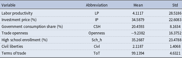
Table 1 lists the 23 manufacturing industries included in our sample, while Table 2 presents the names, means, and standard deviations of the explanatory variables. Additionally, our sample covers the period from 1963 to 2018 and consists of the 20 countries in the Eurozone, including Austria, Belgium, Croatia, Cyprus, Estonia, Finland, France, Germany, Greece, Ireland, Italy, Latvia, Lithuania, Luxembourg, Malta, the Netherlands, Portugal, Slovakia, Slovenia, and Spain.
Manufacturing industries at the International Standard Industrial Classification of All Economic Activities two-digit level, and the numbers of countries of each industry

Summary statistics of the data

5. Empirical results
This section consists of three subsections. In the first subsection (Section 5.1), we discuss results on conditional convergence. In the second subsection (Section 5.2), we analyze results on unconditional convergence. In the third subsection (Section 5.3), we conduct a robustness check using different subperiods.
5.1 Results from the conditional convergence regression
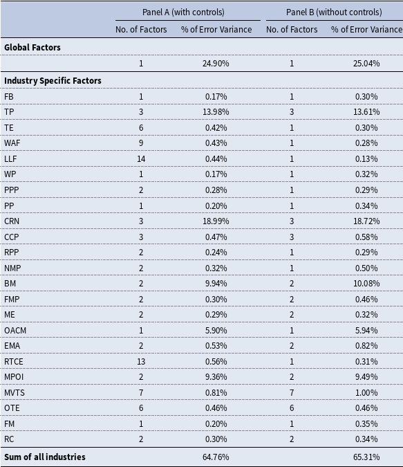
We begin by examining conditional convergence using the constant-coefficient hierarchical panel data convergence regression model in equation (2.1). The first column of Table 3.A. presents the number of unobserved global and industry-specific factors. As shown, we have identified one global factor influencing the growth in labor productivity across every individual manufacturing industry. In terms of industry-specific factors, the number varies across industries, ranging from 1 to 14, with an average of 4.
Estimates of the global and industry-specific factors

To better understand the role of global and industry-specific factors in explaining the total variance of the error terms, represented as
 $(Y_{ij}-X_{ij}\hat {\boldsymbol {\beta }}_{i})$
, we calculate the proportion of the total variance attributed to these two sets of factors. The results are presented in the second column of Table 3.A. As shown in the table, the global factor accounts for 24.90% of the total variance, while the industry-specific factors collectively contribute to 64.76% of the total variance. The contribution of individual industry-specific factors ranges from 0.17% to 18.99%. The significant role played by industry-specific factors highlights that accounting for global factors alone is insufficient for analyzing convergence with multi-level data, emphasizing the need for a hierarchical model.
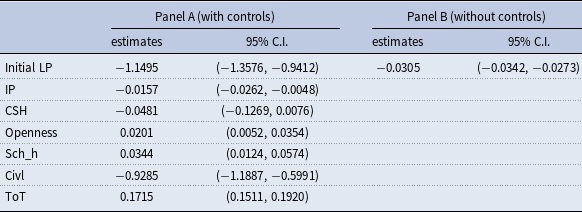
Table 4.A displays the estimated coefficients for the total manufacturing industry. All control variables show expected signs. For example, the coefficient for the price of investment goods is notably negative, suggesting that a lower initial price of these goods in each five-year period correlates strongly and positively with subsequent growth in labor productivity. This finding supports the notion that lower investment costs encourage spending on essential assets, such as machinery and equipment. It also incentivizes firms to adopt new technologies and upgrade their production processes, thereby promoting labor productivity growth (De Long and Summers, Reference De Long and Summers1991, Reference De Long and Summers1992). Moreover, the significantly positive coefficient for high school enrollment aligns with previous research affirming that higher education levels enhance human capital, fostering a workforce adept at adopting new technologies and enhancing productivity (Barro, Reference Barro1991). Additionally, the statistically positive coefficient for trade openness echoes the findings of Coe and Helpman (Reference Coe and Helpman1995), indicating that increased trade openness enables firms to tap into broader markets and cutting-edge technologies, thereby promoting the adoption of efficient production methods and spurring innovation.
Estimated coefficients

The estimated coefficient for initial productivity in the overall manufacturing industry, as presented in Table 4.A, stands at
 $-1.1495$
and is highly significant, with a 95% confidence interval of (
 $-1.3576$
,
 $-0.9412$
). This indicates that, after accounting for country-specific characteristics, higher initial labor productivity negatively correlates with subsequent labor productivity growth. Essentially, this provides evidence of conditional convergence in labor productivity across the total manufacturing sector. This finding echoes Rodrik (Reference Rodrik2013), who also noted conditional convergence in labor productivity for manufacturing. It aligns with the income convergence literature (Islam, Reference Islam1995; Sala-I-Martin et al. Reference Sala-I-Martin, Doppelhofer and Miller2004), which suggests that when country characteristics are considered, the initial income coefficient turns negative and statistically significant.
It is worth noting that our estimated coefficient for initial productivity, at
 $1.1495$
(in absolute value), significantly exceeds the
 $0.018$
reported by Rodrik (Reference Rodrik2013) for 118 countries worldwide. This suggests that Eurozone countries converge at a faster rate in productivity compared to the broader sample studied by Rodrik. Several factors contribute to this accelerated convergence. First, Eurozone countries share a unified monetary policy managed by the European Central Bank, promoting economic convergence by ensuring price stability and supporting investment. Second, deep economic integration and trade among Eurozone members facilitate efficient resource allocation, technology transfer, and economies of scale, fostering productivity convergence. Third, alignment of economic policies and regulations with EU standards reduces trade barriers, promotes competition, and encourages innovation, all enhancing productivity growth and convergence. Fourth, well-developed infrastructure networks in the Eurozone, including transportation, communication, and energy systems, facilitate the movement of goods, services, capital, and labor, thereby reducing transaction costs and improving market access. Fifth, high levels of institutional quality within the Eurozone, such as strong legal frameworks and property rights protection, provide a stable environment for business operations and investment, further fostering productivity growth and convergence.
Furthermore, the disparity in convergence rates between our study and Rodrik (Reference Rodrik2013) may also stem from the following factors. Firstly, while Rodrik (Reference Rodrik2013) employs simple averages derived from four sub-periods for both dependent and independent variables, our analysis utilizes five-year moving averages. Secondly, our regression equation for conditional convergence incorporates both regressors and hierarchical factor structures, whereas Rodrik (Reference Rodrik2013) only includes fixed effects. This discrepancy in model specification could also contribute to the variation in estimated convergence coefficients between Rodrik’s study and ours.
Estimated industry-specific coefficients from the conditional convergence regression

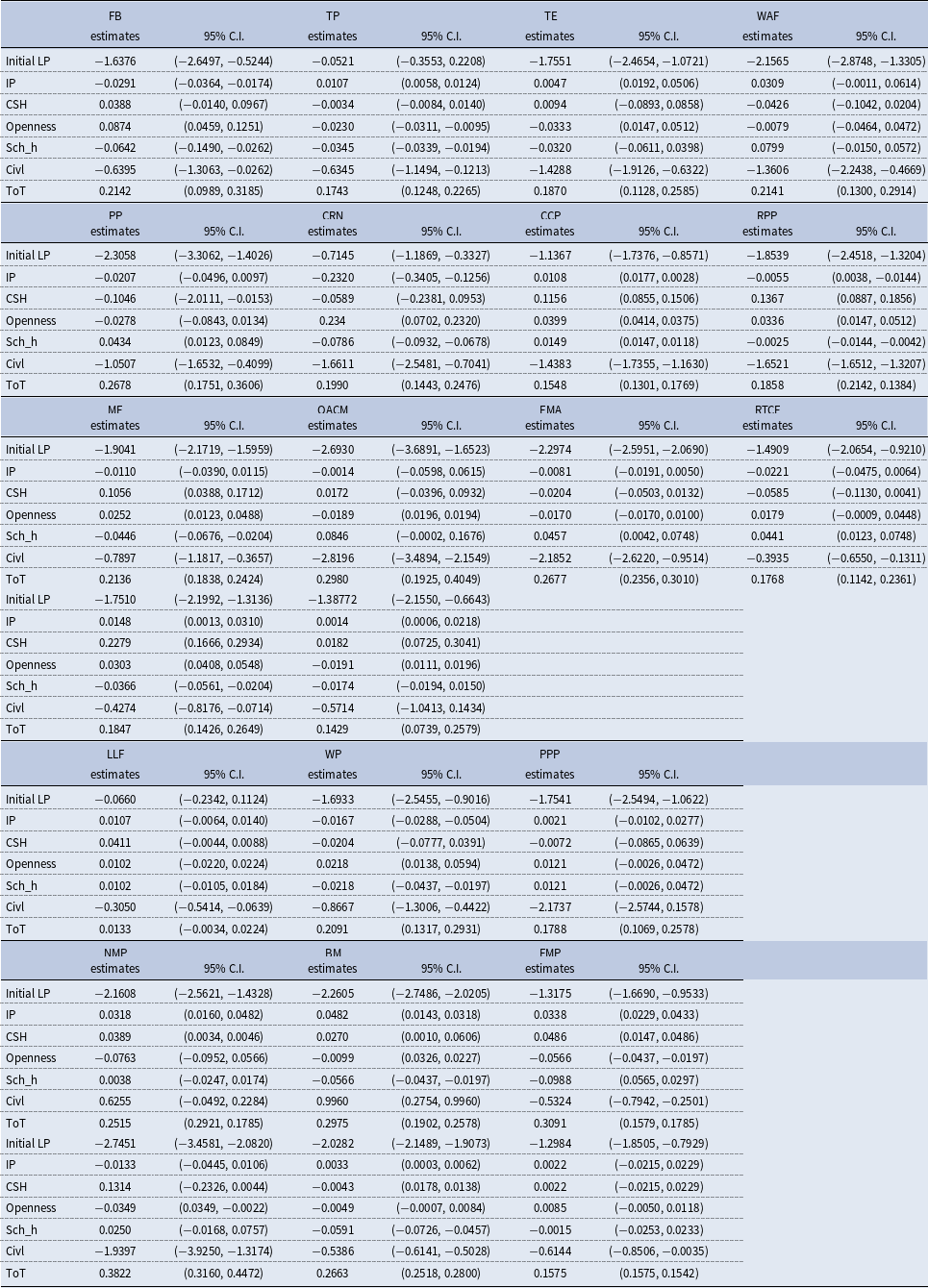
In our final analysis, we evaluate conditional convergence across 23 manufacturing industries using the varying-coefficient hierarchical panel data convergence regression model outlined in equation (3). This model allows for industry-specific coefficients and incorporates all relevant components, including initial productivity, control variables, and hierarchical factors. Table 5 presents the results, which largely align with those observed for the manufacturing sector as a whole. Specifically, of the 23 industries examined, 21 display a significantly negative coefficient on initial productivity, varying from
 $-0.7145$
(CRN, i.e., coke, refined petroleum products, nuclear fuel industry) to
 $-2.7451$
(MPOI, i.e., medical, precision and optical instruments). The only exceptions are TP (tobacco products industry) and LLF (leather, leather products and footwear), where the conditional convergence coefficients are also negative but are not statistically different from zero. These results indicate that almost all individual manufacturing industries exhibit conditional convergence in labor productivity.
5.2 Results from the unconditional convergence regression
Tests for unconditional convergence employ a regression specification similar to that used in conditional convergence tests but omit country characteristic controls (i.e., equation (2.1) without control variables). Initially, we examine results for the total manufacturing industry. Table 3.B provides insights into the number and contributions of global and industry-specific factors in explaining the total error variance. Generally speaking, these findings closely mirror those presented in Table 3.A. A single global factor influences all industries, while industry-specific factors range from 1 to 7 per industry, averaging 2. The global factor accounts for 25.04% of the total variance, and industry-specific factors collectively explain 65.31%, with individual contributions ranging from 0.13% to 18.72%.
In Table 4.B, the estimated coefficient on the initial productivity for the total manufacturing industry is also statistically significant, with a point estimate of
 $-0.0305$
and a 95% confidence interval of (
 $-0.0342$
,
 $-0.0273$
). This implies that, even in the absence of country-specific attributes, higher initial labor productivity is associated with a subsequent decline in labor productivity growth. In other words, there’s evidence of unconditional convergence in labor productivity across the manufacturing sector as a whole, confirming Rodrik (Reference Rodrik2013)’s findings of unconditional convergence in manufacturing labor productivity. This is also consistent with the finding of Mankiw et al. (Reference Mankiw, Romer and Weil1992) that unconditional convergence can occur among a group of relatively homogeneous countries, as in our case.
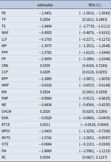
To explore whether this unconditional convergence extends to individual manufacturing industries, we conducted an analysis without control variables using equation (3). Table 6 presents the estimated industry-specific coefficient of initial labor productivity for all 23 manufacturing industries. This coefficient varies significantly across industries, ranging from
 $-2.9050$
(PP, i.e., printing and publishing industry) to
 $0.5559$
(CRN, i.e., coke, refined petroleum products, nuclear fuel industry). Specifically, among the 23 industries examined, 16 exhibit a significantly negative coefficient on initial productivity, ranging from
 $-0.0085$
(OTE, i.e., other transport equipment industry) to
 $-2.9050$
(PP, i.e., printing and publishing industry). 6 industries display a significantly positive coefficient on initial productivity, ranging from
 $0.0209$
(CCP, i.e., other transport equipment industry) to
 $0.5559$
(CRN, i.e., coke, refined petroleum products, nuclear fuel industry), while 1 industry (RTCE, i.e., Radio, television and communication equipment) shows a positive but statistically insignificant coefficient. These results suggest that the majority of individual manufacturing industries exhibit unconditional convergence, with only a few displaying unconditional divergence or an ambiguous relationship between initial productivity and subsequent growth.
Estimated industry-specific coefficients of initial productivity from the unconditional convergence regression

It’s notable that the convergence rate is significantly higher for conditional convergence (
 $1.1495$
in absolute value) than that for unconditional convergence (
 $0.0305$
in absolute value) in the Eurozone. This finding is not surprising. Conditional convergence models, by controlling for factors such as institutional quality, policy environment, and structural characteristics, focus on the convergence process after accounting for initial disparities. In contrast, unconditional convergence models do not account for these factors, leading to a slower convergence rate as they overlook the heterogeneity in initial conditions among Eurozone countries.
5.3 Robustness check
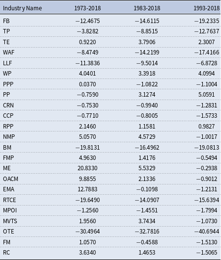
To ensure the robustness of the findings outlined in Subsections 5.1 and 5.2, we conducted a thorough examination using different sample periods. This robustness check involved re-estimating the constant-coefficient hierarchical panel data convergence regression model presented in equation (2) and the varying-coefficient hierarchical panel data convergence regression model presented in equation (3). We performed these estimations both with and without control variables for three distinct subperiods: 1973–2018, 1983–2018, and 1993–2018.
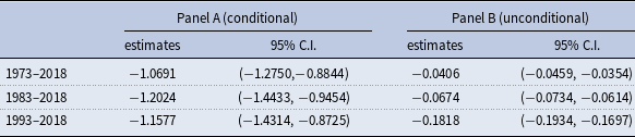
Specifically, equation (2) with control variables was utilized to assess conditional convergence for the total manufacturing industry for the three subperiods, while equation (2) without control variables was employed to examine unconditional convergence. The ensuing results are detailed in Panel A and Panel B of Table 7, respectively. In Panel A of Table 7, the estimated coefficients on initial productivity from equation (2) with control variables are consistently negative and statistically significant for the total manufacturing industry across all subperiods, indicating conditional convergence regardless of the time period. Similarly, Panel B shows that the estimated coefficients on initial productivity from equation (2) without control variables remain consistently negative and statistically significant for the total manufacturing industry across all subperiods, confirming unconditional convergence regardless of the time period.
Estimated coefficients of initial productivity across different subperiods

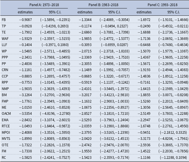
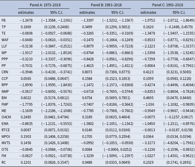
Additionally, we also re-estimated the varying-coefficient hierarchical panel data convergence regression model in equation (3) with and without control variables for the same subperiods. Equation (3) with control variables tests for conditional convergence for individual manufacturing industries, while equation (3) without control variables tests for unconditional convergence. The results are presented in Table 8 and 9, respectively.
Estimated industry-specific coefficients of initial productivity across different subperiods (conditional model)

Estimated industry-specific coefficients of initial productivity across different subperiods (unconditional model)

In Table 8, the estimated coefficients on initial productivity from equation (3) with control variables are consistently negative and statistically significant for the majority of the 23 manufacturing industries across all subperiods, indicating conditional convergence regardless of the time period. Specifically, out of the 23 manufacturing industries, 21 show statistically significant conditional convergence for the subperiod 1973–2018, 21 show statistically significant conditional convergence for the subperiod 1983–2018, while 21 show statistically significant conditional convergence for the subperiod 1993–2018.
Similarly, Table 9 shows that for the majority of the 23 manufacturing industries, the estimated coefficients on initial productivity from equation (3) without control variables remain consistently negative and statistically significant across all subperiods, confirming unconditional convergence regardless of the time period. Specifically, out of the 23 manufacturing industries, 15 show statistically significant unconditional convergence for the subperiod 1973–2018, 14 show statistically significant unconditional convergence for the subperiod 1983–2018, while 16 show statistically significant unconditional convergence for the subperiod 1993–2018.
6. Comparison with other models
In this section, we conduct a more comprehensive robustness analysis by comparing the results of the hierarchical panel model with those derived from two other models commonly used in the convergence literature: the Log t-test proposed by Phillips and Sul (Reference Phillips and Sul2007, Reference Phillips and Sul2009) and conventional panel data regression models, including the pooled panel data model and the fixed effects panel data model. As the findings presented below reveal, the results from the Log t-test are generally consistent with those of the hierarchical panel model. Furthermore, the hierarchical panel model demonstrates superior performance compared to the conventional panel data regression models.
6.1 Comparison with the Phillips and Sul (Reference Phillips and Sul2007, Reference Phillips and Sul2009) Log t Test
The Phillips and Sul (Reference Phillips and Sul2007, Reference Phillips and Sul2009) log t-test is a flexible, nonparametric framework for identifying convergence patterns and detecting club convergence. Based on a time-varying factor model, the test evaluates whether the relative transition paths of individual units converge to a common steady-state trajectory. It involves estimating a regression of the logarithm of the cross-sectional variance of the relative transition parameters over time, with convergence assessed under the null hypothesis using a t-statistic. At the 5% significance level, a critical value of -1.65 is applied, where a t-statistic greater than this value indicates convergence, while a lower value suggests divergence.
6.1.1 Results from the Phillips and Sul (Reference Phillips and Sul2007, Reference Phillips and Sul2009) Log t Test
Since the Phillips and Sul (Reference Phillips and Sul2007, Reference Phillips and Sul2009) log t-test is designed for standard panel data frameworks and is unsuitable for hierarchical data structures, we apply it separately to each of the 23 sub-manufacturing industries, as each exhibits a standard panel structure. Table 10 reports the log t-test results for these industries, showing that 16 out of 23 industries have t-statistics exceeding the critical value of -1.65, providing strong evidence of productivity convergence within these sub-manufacturing industries. These findings align with the results from the hierarchical panel model, as both approaches indicate convergence in most of the sub-manufacturing industries.
T-test statistics for the 23 sub-manufacturing industries

For the seven sub-manufacturing industries (FB, TP, WAF, LLF, BM, RTCE, and OTE) where overall convergence is not observed, we further investigate the possibility of club convergence. The Phillips and Sul (Reference Phillips and Sul2007, Reference Phillips and Sul2009) log t-test can be extended to analyze club convergence by ranking countries based on their transition parameters or growth rates. An iterative log t-test is then applied to subsets of the ranked units to identify clusters where the t-statistic meets or exceeds the critical value of -1.65. Units satisfying the convergence criterion are grouped into a club, and the process is repeated for the remaining units until all potential clubs are identified.
Table 11 presents the results of the club convergence analysis for these seven sub-manufacturing industries. Notably, club convergence is observed in all seven industries, with most countries concentrated in a single dominant club in six of them. For example, in the TP (Tobacco products) industry, two clubs are identified, with one club encompassing 17 of the 20 Eurozone economies. Similarly, in the RTCE (Radio, television and communication equipment) industry, two clubs are identified, with one club including 16 of the 20 Eurozone economies. These findings indicate that while overall convergence is absent in these six industries, majority-driven club convergence is present, offering further evidence of productivity convergence within the Eurozone’s manufacturing industries.
Club convergence analysis for the seven sub-manufacturing industries lacking overall convergence

An identified club must consist of at least two countries. A single country that does not belong to any club or cannot merge with another country is classified as a divergent unit.
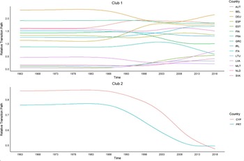
In addition to applying the log t-test to the 23 sub-manufacturing industries, we also follow Phillips and Sul (Reference Phillips and Sul2007, Reference Phillips and Sul2009) by plotting the relative transition paths for each industry. These plots provide a visual means to assess whether individual countries within each industry converge to a common steady-state path or form distinct convergence clubs. Due to space constraints, we present the relative transition paths for two representative industries: (1) wood products (WP), one of the 16 sub-manufacturing industries demonstrating overall convergence, and (2) other transportation equipment (OTE), one of the 7 sub-manufacturing industries exhibiting club convergence. Figure 1 illustrates the relative transition paths for WP, showing heterogeneity across countries but a notable reduction in the dispersion of transition curves over time. This narrowing of curves toward a common steady-state reflects diminishing variance and aligns with the log t-test results, providing clear evidence of overall convergence. In contrast, Figure 2 depicts OTE, where overall convergence is absent, but two distinct subgroups emerge, each converging toward their own steady states, demonstrating clear club convergence.
Relative transition paths for the woods products industry.

Relative transition paths for the other transport equipment industry.

Finally, we apply the Phillips and Sul (Reference Phillips and Sul2007, Reference Phillips and Sul2009) log t-test to three subperiods: 1973–2018, 1983–2018, and 1993–2018, as outlined in Subsection 5.3. Table 12 presents the results for the 23 sub-manufacturing industries across these subperiods. As shown, the t-statistic exceeds the critical value of -1.65 for the majority of the 23 sub-manufacturing industries in all subperiods, indicating convergence for most industries regardless of the time period. Specifically, 16 out of the 23 industries exhibit statistically significant convergence during the 1973–2018 subperiod, 16 during the 1983–2018 subperiod, and 15 during the 1993–2018 subperiod. The finding that convergence occurs in most sub-manufacturing industries, irrespective of the time period, closely aligns with the results from the hierarchical panel model presented in Subsection 5.3, further reinforcing the robustness of the analysis.
T-test statistics for the 23 industries across different subperiods

In summary, the results of the Phillips and Sul (Reference Phillips and Sul2007, Reference Phillips and Sul2009) log t test align closely with those of the hierarchical panel model discussed in Section 5, as both approaches reveal that the majority of the 23 sub-manufacturing industries exhibit convergence. Furthermore, our club convergence analysis indicates that even in industries where overall convergence is absent, most countries are grouped into a single dominant club, providing additional evidence of productivity convergence within the Eurozone’s manufacturing sector.
6.1.2 A comparison between the Phillips and Sul (Reference Phillips and Sul2007, Reference Phillips and Sul2009) method and the hierarchical panel data model in addressing transition paths, common factors, and heterogeneity
While the results from the Phillips and Sul (Reference Phillips and Sul2007, Reference Phillips and Sul2009) log t-test and the hierarchical panel model are generally consistent, it is important to emphasize their key methodological differences in addressing transition paths, common factors, and heterogeneity.
First, the Phillips and Sul (Reference Phillips and Sul2007, Reference Phillips and Sul2009) method and the hierarchical panel data model differ in their treatment of transition paths and long-term dynamics. The Phillips and Sul method explicitly accounts for transition paths and long-term dynamics through its use of a time-varying factor model that tracks the relative transition paths of individual countries in a panel. By normalizing each country’s trajectory relative to the group average, the method captures dynamic adjustments over time, enabling the identification of whether countries converge to a common steady-state path. For example, in Section 6.1.1, Figure 1 illustrates that in the wood products (WP) industry, individual countries show a progressive narrowing of relative transition paths over time, signifying overall convergence toward a shared steady-state trajectory. In contrast, Figure 2 reveals that in the other transport equipment (OTE) industry, where overall convergence is not observed, the relative transition paths form distinct subgroups, providing clear evidence of club convergence dynamics.
In contrast, our hierarchical panel model, grounded in beta convergence, captures long-term dynamics by linking initial productivity levels to subsequent growth rates, reflecting adjustments toward a steady-state equilibrium over time. This approach provides insights into both the speed of convergence and the progress in closing productivity gaps. For example, the results in Section 5 reveal that the manufacturing sector as a whole and most of the 23 sub-manufacturing industries exhibit a negative relationship between initial productivity levels and subsequent growth rates, signaling a gradual movement toward their respective steady states. However, while this method effectively models long-term convergence trends, it does not explicitly capture the dynamic transitional paths emphasized in Phillips and Sul’s framework, highlighting the complementary of the two approaches in analyzing convergence processes.
Second, the Phillips and Sul (Reference Phillips and Sul2007, Reference Phillips and Sul2009) method and the hierarchical panel data model differ in how they handle common factors. The Phillips and Sul (Reference Phillips and Sul2007, Reference Phillips and Sul2009) method decomposes panel data into a common growth factor shared by all units and idiosyncratic deviations unique to each unit. The common growth component captures shared dynamics or shocks, while relative transition paths track individual deviations. By analyzing cross-sectional variance over time, the method implicitly captures the influence of the common growth component without explicitly modeling its form. As a result, the Phillips and Sul (Reference Phillips and Sul2007, Reference Phillips and Sul2009) method does not explicitly estimate common factors and their loadings.
In contrast, the hierarchical panel model adopts a more explicit and structured approach by incorporating two sets of latent common factors: global factors, which capture dependencies at the manufacturing level, and industry-specific factors, which account for dependencies within sub-manufacturing industries. This framework allows for the explicit estimation of both common factors and factor loadings. For instance, in Section 5, we not only identified the number of factors but also estimated the corresponding common factors and factor loadings. In this way, our explicit estimation of latent factors and their loadings complements the implicit dynamics modeled within Phillips and Sul’s framework.
Finally, the Phillips and Sul (Reference Phillips and Sul2007, Reference Phillips and Sul2009) method and the hierarchical panel model take distinct approaches to addressing heterogeneity. The Phillips and Sul method employs a nonlinear factor model with time-varying idiosyncratic components, enabling each unit to exhibit unique transitional dynamics relative to a common growth trajectory. By focusing on relative transition paths, the method identifies convergence clubs—subgroups of units that converge to their own distinct steady states rather than the overall average. For instance, in Section 6.1.1, we identified seven sub-manufacturing industries where countries exhibit convergence to different steady states.
In contrast, the hierarchical panel model captures heterogeneity by allowing coefficients to vary across sub-manufacturing industries, enabling each industry to follow a distinct and industry-specific convergence trajectory. For instance, as shown in Section 5, the estimated coefficients on initial productivity differ significantly across the 23 sub-manufacturing industries, indicating that each industry exhibits a unique convergence path. It is important to note that the hierarchical panel model and the Phillips and Sul (Reference Phillips and Sul2007, Reference Phillips and Sul2009) method address different dimensions of heterogeneity. The former focuses on heterogeneity across sub-manufacturing industries within a three-dimensional panel data framework, while the latter emphasizes heterogeneity across countries in a standard two-dimensional panel data setting.
6.2 Comparing with conventional panel data models
In this subsection, we compare the proposed hierarchical panel model with two conventional panel data models—the fixed effects panel data model and the pooled panel data model. To address space limitations and effectively highlight the advantages of the hierarchical panel model, our analysis focuses exclusively on the total manufacturing industry within the context of conditional convergence. This focus is well-suited for illustrating the hierarchical panel model’s ability to manage hierarchical data structures, while the examination of conditional convergence underscores the model’s effectiveness in estimating the coefficient on initial productivity and other control variables.
6.2.1 Statistical performance of the three models
We begin by evaluating the statistical performance of the fixed effects, pooled, and hierarchical panel models using the Bayesian Information Criterion (BIC), Akaike Information Criterion (AIC), and residual diagnostics through Pesaran’s cross-sectional dependence (CD) test for cross-sectional dependence. As shown in Table 13, the hierarchical panel model outperforms the others, achieving the lowest BIC (238660.9) and AIC (238604.0), which reflects its superior ability to balance model fit and complexity. In contrast, the fixed effects and pooled models yield higher BIC values (239348.5 and 240190.3) and AIC values (239291.6 and 240117.1), underscoring their limitations in capturing the underlying complexities of the data.
Goodness of fit and cross-sectional dependence test for the three competing models

The numbers in the table represent the count of sub-manufacturing industries belonging to the corresponding clubs. OLS: Ordinary Least Squares.
Furthermore, residual diagnostics from Pesaran’s CD test confirm the robustness of the hierarchical model, with no significant cross-sectional dependence detected (p-value = 0.28), whereas both conventional models exhibit strong residual dependence (p-value = 0.00). These results underline the importance of addressing CSD and heterogeneity in analyzing productivity convergence.
6.2.2 Productivity results: hierarchical model vs. Conventional models
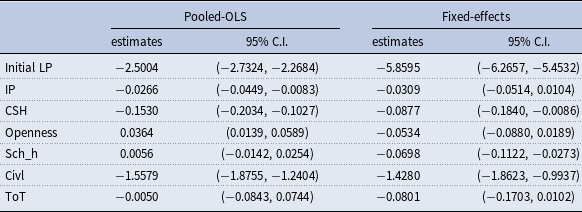
Table 14 presents the estimated coefficients from the fixed effects and pooled models. Both models provide evidence of conditional convergence in the manufacturing industry as a whole, as reflected by the negative and statistically significant coefficients for initial productivity. However, the convergence rates estimated by these models are substantially higher than that of the hierarchical panel model. Specifically, the fixed effects model yields a convergence rate of 5.8595 per year, while the pooled model estimates a rate of 2.5004 per year, compared to the lower rate of 1.1495 per year produced by the hierarchical panel model.
Estimated coefficients for the pooled-OLS and fixed-effects models

This discrepancy can be attributed to two key factors. First, the fixed effects and pooled models fail to account for cross-sectional dependence at both the aggregate manufacturing and sub-manufacturing levels. Ignoring these interconnections can introduce bias into the convergence estimates, leading to potentially misleading conclusions (Andrews, Reference Andrews2005; Phillips and Sul, Reference Phillips and Sul2007). Second, both models impose constant coefficients across industries, disregarding the varying adjustment speeds that naturally exist among different sub-manufacturing industries.
In addition to differences in convergence rates, we observe discrepancies in the estimated coefficients for some control variables between the fixed effects and pooled models and the hierarchical panel model. Specifically, the fixed effects and pooled models produce coefficients for certain control variables that deviate substantially from those estimated by the hierarchical panel model and, in some cases, lack theoretical plausibility. For instance, the fixed effects model estimates a negative coefficient for trade openness, implying that higher trade openness is associated with slower productivity convergence—an outcome that contradicts established economic theory. Similarly, the pooled model estimates a statistically insignificant coefficient for high school enrollment, failing to capture the critical role of education in driving productivity growth. These inconsistencies likely result from the inability of the fixed effects and pooled models to account for cross-sectional dependence and varying coefficients across sub-manufacturing industries, leading to biased and unreliable estimates. In contrast, the hierarchical panel model produces coefficients that align more closely with theoretical expectations, further underscoring its robustness and reliability.
In summary, the fixed effects and pooled models underperform relative to the hierarchical panel model due to their failure to address cross-sectional dependence and heterogeneity. Specifically, the hierarchical model excels across all key statistical metrics, including BIC, AIC, and Pesaran’s CD Test. Additionally, the fixed effects and pooled models produce inflated convergence rates compared to that produced by the hierarchical model. Furthermore, the coefficients for control variables in the conventional models often lack theoretical plausibility. These results underscore the robustness and reliability of the hierarchical panel model in accurately and comprehensively capturing productivity dynamics.
7. Conclusion
In this study, we investigate the conditional and unconditional convergence in labor productivity within the manufacturing industries of the Eurozone, spanning the period from 1963 to 2018. This is done by employing a sophisticated framework of constant and varying-coefficient hierarchical panel data convergence regression models with two sets of latent factor structures: one set of global factors and one set of industry-specific factors. The first set of latent factors impacts all manufacturing industries across all countries while the second set of latent factors affects a subset of sub-manufacturing industries These models offer two advantages, allowing for both global and industry-specific cross-sectional dependencies and accommodating coefficients that vary across individual industries.
Our findings offer compelling evidence of both conditional and unconditional convergence within the manufacturing industry as a whole, as well as among the majority of its sub-industries. Moreover, our analysis reveals significant variation in convergence patterns across sub-manufacturing industries, underscoring the importance of industry-specific approaches in understanding productivity dynamics. Robustness checks conducted using different subperiods further confirm these results. Lastly, a comparison of our model’s results with those of two alternative models offers additional validation for our conclusions.