

1. Introduction: the controversy over agrarian protectionism
When international grain prices fell and imports of grain into Western Europe sharply increased in the 1870s and 1880s, it caused falling profitability for grain producers and reduced land prices in West European countries. The grain invasion provoked different responses in different countries. While some countries, notably Denmark and the UK, stuck to free trade in agricultural commodities, others, such as France, Germany and Sweden, imposed tariffs to protect landowners. According to Kevin O'Rourke (Reference O'Rourke1997), the varying responses to the grain invasion depended on its impact on land rents and the role of agriculture in national economic life. In the UK the weight of the agricultural sector in the national economy was already much reduced and in Denmark farmers were already well on their way in switching over to animal produce. In contrast, on the European continent cereal production was much more important. The response to the grain invasion probably also had something to do with the political clout of landowners. In a classical study Alexander Gerschenkron (Reference Gerschenkron1943) argued that in Germany agrarian protectionism only benefited a minority of relatively large landowners specializing in bread-grain production. According to Gerschenkron, small farmers did not gain much from agricultural protection even though they produced grain, since they used their grain produce primarily for their own consumption and for fodder. Against Gerschenkron, Steven Webb (Reference Webb1982) has argued that the output mix did not differ much between small farms and large farms and that animal produce also received substantial tariff protection in Germany.
In Sweden as in Germany, the campaign for grain tariffs was primarily conducted by large landowners, specializing in bread-grain production. The majority of small farmers typically specialized in animal husbandry, which was much less exposed to overseas competition. Agrarian protectionism was filled with controversy from the beginning. In the debates on trade policy in the 1880s critics pointed out that grain tariffs primarily served the interests of large landowners in southern and central-eastern Sweden, specializing in producing bread-grain. In answer, to win over the majority of small farmers, the protectionists also campaigned for the introduction of tariffs on maize and pork. Maize was considered a substitute for oats in the feeding of pigs, and adherents of protectionism argued that the maize tariff would primarily benefit small farmers since oats were their most important crop. However, as free traders pointed out, pig farming was also more important for small and middle-sized farms than for large farms, and the feeding of pigs was made more expensive by the maize tariff. Moreover, the most important source of revenue for small farmers derived from milk, which was unprotected (Gellerman Reference Gellerman1958, pp. 17–43).
After intense debates over tariffs in the 1880s, the controversy faded during the general economic upswing in the 1890s, when the protectionist system had been settled. A new controversy over food tariffs was again brought to the fore around 1910. Many male workers now had a yearly income exceeding 800 kr and had thereby gained the right to vote in parliamentary elections. Accordingly, the Social Democrats could now muster a sizable representation in the parliament. Increasing unemployment in the wake of the economic crises in 1907 resulted in hardships for many workers. Food tariffs, in particular grain tariffs, were now singled out for critique by the Social Democrats in alliance with the so called Norrland liberals, representing small farmers from northern Sweden, where grain production had always been of marginal importance. However, the critique of grain tariffs proved to be half-hearted since the Social Democrats feared that abolishing agricultural tariffs would lead to demands from farmers for the dismantling of tariffs also on industrial products. Since many industries were dependent on tariffs, the Social Democrats feared that their withdrawal would lead to increased unemployment. In addition, grain tariffs were now an important source of revenue for the government and it was believed that their withdrawal would lead to a fiscal crisis. This would in turn have necessitated compensatory increases in other taxes. A firm stance against agrarian protectionism was also prevented by differences among Social Democrats on the issue. Many small farmers had now joined the party and they were generally in favour of agrarian protectionism.
The only practical result of the renewed controversy over agrarian tariffs was that the maize tariff was abolished in 1911. Critics of food tariffs were hampered by lack of factual knowledgeFootnote 1 of conditions in agriculture and the probable impact of dismantling agrarian tariffs on different farmers. Data collected in the 1910s and the early 1920s have improved our knowledge of the output mix of farms of different sizes, which makes it possible to answer some of the issues at stake in the contemporary debates on food tariffs before World War I.
The purpose of this article is to explore the income distributional consequences of agrarian tariffs in Sweden before World War I. Did agrarian and food tariffs benefit only a minority of relatively large landowners specializing in bread-grain production, or did the majority of small farmers also profit from them, and how did they affect real wages of urban workers and the rate of return on capital in the manufacturing industry? The fact that social strata with opposing material interests played an important role in the shaping of trade policy has long since been recognized by political scientists (Rogowski Reference Rogowski1989), but what has been lacking from this literature is a quantitative assessment of the impact of tariffs on different social classes and strata. This article joins the earlier examples of economic historians such as Webb (Reference Webb1982) and O'Rourke (Reference O'Rourke1997) in trying to make such an assessment. Sweden makes an interesting intermediate case between high-protectionist countries such as Germany and France and free-trade countries such as Denmark. In Sweden high tariffs were imposed on bread-grain, but not on oats, the most important crop for the majority of farmers who increasingly converted their output in the direction of more animal produce.
In the next section I outline some of the main features of agricultural development in Sweden in the late nineteenth and early twentieth centuries. Thereafter, I show how the output of crop products and animal produce was distributed between farms of different sizes on the eve of World War I, and present data on the varying extent to which these farms benefited from agrarian protectionism. In the final section the distributional impact of agrarian tariffs is explored by means of a Computable General Equilibrium model, calibrated with data from 1913.
2. Swedish agriculture in 1870–1913, bread-grain protection and increasing specialization in animal produce
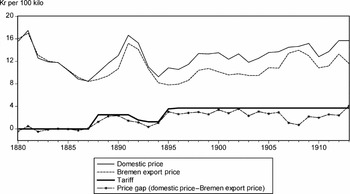
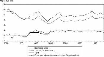
The perhaps most visible sign that the world economy had entered an era of globalization in the late nineteenth century was the emergence of an international grain market that determined grain prices in each corner of the world. To stem the competition from overseas grain, landowners campaigned for the reintroduction of grain tariffs. In 1888 the protectionists won the majority in the Swedish parliament and tariffs on bread-grain and flour were introduced as well as tariffs on animal food products (Bohlin Reference Bohlin2005). The tariff on barley, rye and wheat was set to 2.5 kr per 100 kilo, while oats were protected by 1 kr per 100 kilo. When international grain prices rose at the beginning of the 1890s, tariffs on barley, rye and wheat were lowered to 1.25 kr per 100 kilo in 1892, while the tariff on oats was abolished. Thereafter world market prices fell again. To protect Swedish producers, the tariff on barley, rye and wheat was raised to 3.70 kr in 1896, and stayed unchanged thereafter. For barley and rye, the specific tariff on bread-grain translated into an ad valorem protection of 30–35 per cent for most years, while the protection for wheat was somewhat lower due to its higher price. Tariffs on flour were introduced concomitantly with grain tariffs. In 1888, a tariff of 4.30 kr per 100 kilo was imposed on flour. It was lowered to 2.50 kr per 100 kilo in 1892 and raised to 6.50 kr per 100 kilo in 1896, which amounted to an ad valorem tariff of 40–45 per cent for most years.
The impact of the bread-grain tariff on Swedish grain prices can be seen from Figures 1 and 2, showing the evolution of world market prices and domestic prices for rye and wheat, and the extent to which the tariff drove a wedge between world market prices and domestic prices. Swedish producers more or less entirely utilized the tariff on wheat (Figure 2), whilst for rye the price gap between Swedish and world market prices did not make up the whole tariff (Figure 1). Especially when world market prices rose, as they did between 1905 and 1910, the gap between Swedish and world market prices in rye diminished.
Rye, domestic price and Bremen export price
Source: Åmark (Reference Åmark1924, pp. 118–26).
Note: Prices are yearly averages of monthly prices. Domestic prices are averages of prices in Stockholm and Malmö.


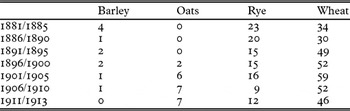
The grain tariff thus succeeded in elevating Swedish grain prices above world market prices. After grain tariffs were introduced in 1888, the export of Swedish bread-grain virtually ended, since producers profited more by selling in the protected home market. For rye, the grain tariff also led to a decline in the share of imports in the home market. The import penetration ratio in rye declined from over 20 per cent in the early 1880s to 12 per cent in 1911/13 (Table 1). Demand for wheat was more income elastic than for rye, but the Swedish climate and soil quality were generally less suited for growing wheat. Only on the plains of Scania and central-eastern Sweden was it profitable to grow wheat to any extent, despite the fact that tariffs made it possible for Swedish wheat producers to obtain prices which were 25–30 per cent above world market prices. Consequently, the import penetration ratio in wheat increased from 30–35 per cent in the 1880s to about 60 per cent around the turn of the century. Thereafter, Swedish producers were able to increase their market share to about 50 per cent of the domestic market on the eve of World War I (Table 1).
Import penetration ratio (%) of the domestic market for grain, 1881/85–1911/13

Sources: Lindahl et al. (Reference Lindahl, Dahlgren and Kock1937, pp. 30–7, table 66).
Note: The import penetration ratio is calculated as imports /(domestic output − exports + imports).
Animal produce also received protection. Tariffs on livestock were low and quite inconsequential, however, since transport costs and quarantine rules made for low trade volumes anyhow. More important was the tariff on pork of 0.20 kr per kilo, amounting to an ad valorem tariff of about 20 per cent. The most important animal product, milk, was free of duty. It may be argued that milk producers enjoyed protection since the dairies, a major market for milk producers, were protected by a specific tariff on butter and margarine of 0.20 kr per kilo, translating into an ad valorem tariff protection of about 15 per cent for dairy products (Bohlin Reference Bohlin2005). However the butter tariff was largely inconsequential, since most Swedish butter was exported and the Swedish butter price was more or less the same as the world market price (Jörberg Reference Jörberg1972, p. 211). Denmark was the leading exporter of butter at the time (Henriksen and O'Rourke Reference Henriksen and O'Rourke2005). A comparison of Swedish and Danish prices of butter of similar quality show that they seldom deviated by more than 2–3 per cent.Footnote 2
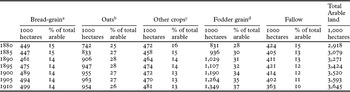
Bread-grain tariffs may have caused an increase in cereal acreage in Sweden, in contrast to Britain and Denmark, who adhered to free trade (O'Rourke Reference O'Rourke1997, table 4). That tariffs influenced farmers’ choice of output mix can be seen clearly if we compare regions in Scania in southern Sweden with regions in neighbouring Denmark with similar climate and soil quality. In Scania, wheat growing expanded after the imposition of grain tariffs, while it declined in the Danish regions. In the Swedish regions bread-grain output increased its share of the total acreage from slightly below 15 to about 20 per cent from the 1870s to World War I, while in the Danish regions it declined from 15 to about 10 per cent. By contrast, fodder grain output and animal produce increased more in the Danish regions (Höijer Reference Höijer1921a, p. 13). However, the most salient feature of Swedish land use in the late nineteenth century is not that the area devoted to bread-grain production increased, but the much stronger increase in cultivated land used for growing fodder grains and green fodder of various sorts. Reclaimed land and land converted from meadows to arable was primarily used to produce fodder for the animals. These tendencies are clearly visible from Table 2. The bread-grain acreage increased by 11 per cent between 1880 and 1910. At the same time, the acreage devoted to the growing of oats, which was primarily used as fodder, increased by 28 per cent, and the fodder grain acreage increased by 62 per cent. The area occupied by meadows declined by 33 per cent between 1880 and 1910 (Höijer Reference Höijer1921b).
Distribution of total arable land in Sweden, 1880–1910 (1,000 hectares) among different uses

Source: Höijer (Reference Höijer1921b, pp. 18–20, table 14a).
Notes:
a Rye and wheat.
b Oats and mixed grain (a mixture of oats and rye, which was used for animal fodder).
c Barley, beans and peas, potatoes and other root crops, textile plants.
d Cultivated crops used for producing hay and for grazing.
To sum up, the percentage of the total cultivated acreage devoted to animal fodder increased from 57 to 63 per cent between 1885 and 1913, while at the same time the bread-grain acreage declined from 15 to 14 per cent. Swedish agricultural statistics on cultivated land have been accused of overstating the increase in the cultivated acreage in the late nineteenth century (Holgersson Reference Holgersson1974). However, in 1910 and probably also in the 1890s it should be fairly accurate.Footnote 3 It is also agreed that the percentage distribution of land between different crops is more accurate than the estimate of the total cultivated acreage.Footnote 4 The trend in land use is anyhow unmistakable, and corrected numbers of the cultivated area would most likely show an even slower growth in the area devoted to bread-grain.
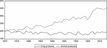
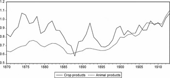
The change in the distribution of land use towards more fodder grains must be seen against the background of an ongoing transformation of Swedish agriculture in the direction of more animal produce. While the volume of crop products for sale outside the agricultural sector stagnated or even declined after 1870, the volume of animal produce increased by 2.3 per cent per year between 1870 and 1913, as is visible from Figure 3. Prices for animal products did not decline nearly as much as for crop products from the 1870s to the 1890s (Figure 4). When prices of crop products increased in the 1890s the prices of animal produce followed suit. Of even more importance than prices for the increasing specialization in animal produce was the fact that the income elasticity of demand for animal products was much higher than for crop products. In addition, milk, the major product of Swedish animal husbandry, also benefited from increased export demand, since it was indirectly exported in the form of butter. Butter was a major export item at the time (Staffansson Reference Staffansson1995, pp. 99 ff.). Its share of total Swedish exports was 10–13 per cent at its height in the 1890s, but after the turn of the century butter exports stagnated and its relative share of Swedish exports sank to about 5–7 per cent.Footnote 5
Volume of crop products and animal produce in Swedish agriculture, 1870–1913
Source: Unpublished data underlying graph 3 in Schön (Reference Schön1995, p. 61), provided by Lennart Schön.
Note: It should be noted that the volumes include only products for sale outside the agricultural sector. For example, grain produced for seeds or animal fodder is not included in the volume of crop products, and milk used for feeding animals is not included in the volume of animal produce.

Prices for crop products and animal products (1913 = 100)
Source: Animal products and crop products, implicit price indices calculated from unpublished data provided by Lennart Schön; see Figure 3 above.

3. Output mix and effective protection for farms of different sizes
3.1. Distribution of land and output mix among farms of different sizes
Data collected in the 1910s and the early 1920s have improved our knowledge of the output mix of farms of different sizes, which makes it possible to answer some of the issues at stake in the contemporary debates on food tariffs before World War I. From a special investigation from 1919 we have information on the distribution of cultivated land on farms of different sizes, measured by cultivated acreage. We also have information on the number of animals of various sorts on these farms. From these data it is possible to obtain estimates of the output of crops and animal products on farms of different sizes in 1913.Footnote 6
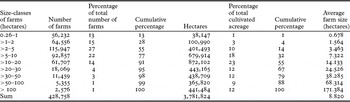
Table 3 reveals that the distribution of land among farms was unequal. The majority of farms cultivated an acreage that was smaller than 5 hectares. Of all farms 77 per cent were smaller than 10 hectares. They cultivated about one-third of the total acreage. Measured in cultivated acreage, only 2 per cent of the farms were larger than 50 hectares, but they cultivated about 20 per cent of the total acreage.
Distribution of farms on various size-classes (hectares) and the cultivated acreage per size-class, Sweden 1919

Source: Höijer (Reference Höijer1921b, pp. 62–5, table 14).
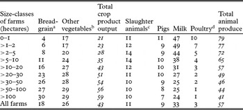
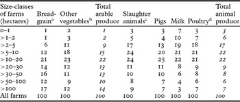
The output mix of crops and animal products of various sorts among farms of different sizes is shown in Table 4. Small farms (up to 10 hectares) clearly specialized in animal produce. Grain output on these farms was largely complementary to animal output, since it consisted predominantly of oats, which were mainly used to feed the animals. Production of bread-grain was of marginal importance on small farms. In contrast, for the larger farms cultivating land of more than 30 hectares bread-grain accounted for about 30 per cent of total output.
Percentage distribution of output (%) on farms of different sizes

Sources: See Appendix 1.
Notes:
a Barley, wheat, rye and other crops protected by tariffs, i.e. sugar beet, peas and beans.
b Oats, mixed grain (a mixture of rye and oats used for feeding animals) and potatoes. These crops were not protected by tariffs.
c Horses, cattle, sheep and goats.
d Hens for slaughter, chickens and eggs.
The different roles of arable and animal products on farms of varying sizes also emerge clearly from Table 5, showing how much of total output of various products was supplied by farms of different sizes. Production of bread-grain was largely concentrated in large farms. Of total bread-grain output, small farms (up to 10 hectares) produced only 20 per cent. If we consider only wheat farming, small farms were of even less importance; of total wheat output they only produced about 10 per cent. Small farms on the other hand accounted for almost 60 per cent of milk output.
Distribution of agricultural output (%) on farms of different sizes

Sources: See Appendix 1.
Notes: See Table 4.
The much more important role for bread-grain production on large farms is also confirmed by Ernst Höijer (Reference Höijer1921c) in a report commissioned by the public investigation committee on the tariff system, appointed after World War I. Höijer explored the extent to which farms of different sizes were able to produce enough bread-grain to provide for the consumption by family members and hired farm-hands between 1913 and 1919. He calculated that people with farms of up to 5 hectares were dependent on purchasing bread-grain to cover their deficits, while farms of between 5 and 10 hectares barely covered their consumption from their own production. Only large farms, over 30 hectares, produced sizable marketable surpluses of bread-grain. According to Höijer's estimate, more than half of the countryside population was dependent on purchase from larger farms for their consumption of bread-grain.
3.2. Effective protection for farms of different sizes
We have seen that the rate of protection varied considerably between different agricultural products. Since farms of different sizes specialized in different kinds of products they did not benefit to the same degree from the protectionist system. Of concern for the farmers was not only the tariff protection they received on their own produce, but also the extent to which their costs increased because of tariffs that they might have to pay on purchased inputs. If tariffs increased their revenues by a higher percentage than the cost of their purchased inputs, they gained from the protectionist system. The rate of effective protection gauges by how much value added increases compared to a hypothetical situation of free trade (Corden Reference Corden1971).
The following formula is used to calculate effective protection rates:  , where gj stands for the effective protection rate on product j, tj and ti are nominal protection rates on products j and i, and aij is an input–output coefficient showing the cost share of i in producing a unit of product j. It shows that effective protection rates rise above/fall below nominal protection rates if the nominal protection rate is higher/lower than the sum of input tariffs multiplied by their input–output coefficients, the more so the larger the share of costs in the value of output.
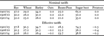
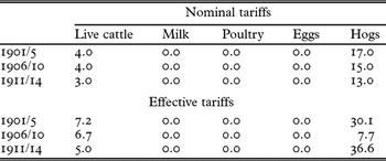
In calculating effective protection rates I have assumed that fertilizers were the only purchased inputs in arable production and that concentrated fodder of various sorts, such as oats, hay and oil-seed cakes, were the only purchased inputs in animal production. My estimates of nominal and effective tariff protection for various agricultural products are displayed in Tables 6 and 7.
Nominal and effective protection for crop products (%) 1901/5–1911/14

Sources: See Appendix 1.
Nominal and effective protection for animal products (%), 1901/5–1911/14

Sources: See Appendix 1.
Effective protection rates were generally higher than nominal protection rates. Since the share of costs for purchased fertilizers in the sales value of grain only amounted to 5–10 per cent or less and the tariff rate on fertilizer was quite low (4–5 per cent), the difference between the nominal and the effective protection rate was not large for grains. For oats and potatoes the effective protection rate was even slightly negative since they were unprotected, while the farmers’ costs for fertilizers were raised by tariffs.
In animal produce it was only the production of hogs that was protected to a substantial extent, but the maize tariff also made the feeding of hogs more expensive. In 1901/6 the maize tariff of 1.25 kr per 100 kilo amounted to an ad valorem tariff of 11–13 per cent. When in 1906 the tariff on maize, the price of which had declined relatively to oats, was raised to 3.7 kr per 100 kilo, the effective protection of hog production was sharply reduced. However, it was still positive, since even if the maize tariff was now higher than the tariff on hogs the cost share of maize was still slightly below 70 per cent of the output value, meaning that tariffs still raised output price more than total costs. The reduced effective protection was not enough to stimulate production and output from hogs fell, leading to increased import penetration of pork. In 1908 the maize tariff was reduced to 1.5 kr per 100 kilo, after which it was abolished in 1911. The dismantling of the maize tariff stimulated Swedish pig farming. Import penetration of pork fell and Swedish producers captured a larger share of the home market.
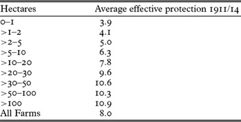
To sum up, Table 7 shows clearly that, with the notable exception of pig farming, animal produce was considerably less protected than arable produce. By putting together information gathered in Tables 5, 6, and 7 we may calculate the rate of protection for farms in different size-classes in 1911/14. The results from such a calculation are displayed in Table 8.Footnote 7
Average effective protection (%) for farms of different sizes 1911/14

Note: The effective protection rate for each size-class is a weighted average obtained by multiplying the product-specific effective protection rate by its share of total value added in each size-class.
Since in Sweden the share of unprotected goods, such as oats and milk, was much more important in the output mix of small farms than of large farms, we may conclude that the majority of small farmers benefited to a much smaller degree than large farmers from agricultural protectionism. The data presented so far explain why owners of large estates were the most ardent supporters of agrarian protectionism. Large landowners also succeeded in rallying support for tariffs from small farmers, as owners of small farms would also lose revenues from a withdrawal of tariffs, although not to the same extent as large farmers. However, counterfactual speculations of this sort do not take into account that the level of output and the output mix would hardly have stayed unchanged after a tariff reform. As a result of tariff changes prices would have changed, not only agricultural and food prices but all prices, not the least factor prices. Changes in relative prices would in their turn have affected resource allocation, which would have affected product prices and so forth. These issues will be explored in a general equilibrium framework in the following sections.
4. A Computable General Equilibrium model of the Swedish economy in 1913
The general idea behind a Computable General Equilibrium model (CGE model) is the interdependence of an economic system. Changes in one market will have repercussions on all markets. A CGE model has four types of exogenous variables: endowments, technology, consumer preferences, and policy variables such as taxes of various sorts. Endowments and technology determine the economy's production possibility frontier. The technology of a sector, expressed by a production function, specifies how inputs may be combined to produce output. Cost functions derived from production functions generate demand functions for the factors which are owned by agents who receive income from their ownership and use these incomes to buy goods guided by their preferences.Footnote 8
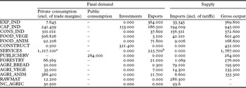
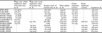
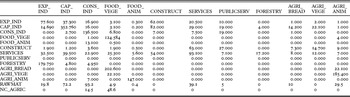
To be usable for analysing real problems, the abstract CGE model must be calibrated with data for a real economy in a benchmark year, in which the economy is assumed to be in a state of general equilibrium. When exogenous parameters are changed, a new equilibrium in the model economy will be established by the altering of relative prices. Concomitantly, factors of production will be reshuffled between the sectors and output levels of the various sectors will change. In order to analyse trade policy issues, I have constructed a model of the Swedish economy in 1913, which is used to explore what happens to factor prices when agricultural and food tariffs are removed. The empirical backbone of the model is a Social Accounting Matrix (SAM), exhibited in Appendix 2 (Tables A2.1, A2.2 and A2.6).
There are twelve producing sectors in the model, seven of which do not produce agricultural goods and food: export industry (EXP_IND),Footnote 9 capital goods industry (CAP_IND), consumer goods industry (CONS_IND), Forestry (FORESTRY), building and construction (CONSTRUCT), private services (including housing, transport and communications) (SERVICES), public services (PUBLICSERV). To explore the impact of agrarian tariffs, I have subdivided the agricultural sector into three sectors: a bread-grain sector (AGRI_BREAD),Footnote 10 a sector producing other arable products (AGRI_VEGE) and a sector producing animal products (AGRI_ANIM).Footnote 11 For the same purpose, I have also subdivided the food industry into two sectors: a sector producing animal food products (FOOD_ANIM)Footnote 12 and another sector using bread-grain, vegetables and other crop products as inputs (FOOD_VEGE). In addition, two sectors of non-competitive imports have been included in the model to account for goods consumed but not produced in Sweden, namely non-competing capital goods and raw materials (RAWMAT),Footnote 13 and non-competing agricultural goods (NC_AGRIC).Footnote 14
Each sector uses intermediate goods in fixed proportions to value added, that is the elasticity of substitution between intermediate goods and the value-added aggregate is zero (the Leontieff technology assumption). Capital and labour in combination produces value added. As is customary in CGE models, it is assumed that the ‘technology’ can be described by a Constant Elasticity of Substitution (CES) production function.
There are two types of labour in the model: urban and rural. It can be shown that in the real world wage rates for labour of the same kind differ persistently between sectors. These differences may be caused by variations in the composition of skill and gender, and institutional factors such as varying bargaining powers of capital and labour. To model the persistence of such ‘wage distortions’ I have assumed that relative wages between sectors do not change for labour of the same kind. The wage rate in a sector is always a given proportion of the average wage for all workers in the same labour category. To give an example: from Table A2.2 it can be calculated that the wage rate in the CAP_IND sector (wage sum divided by number of urban employees in that sector) was 16 per cent higher in 1913 than the average wage for all urban employees, whilst the wage rate in the CONS_IND sector was 20 per cent lower. This wage differential is kept throughout all simulations. Shifts in the demand and supply curves affect the price of labour and alter the relative price of urban and rural labour, but the wage structure for labour of the same kind stays intact.Footnote 15
The possibility to reallocate factors of production is limited in the short run. While labour moves between sectors, capital goods do not. Once an investment has been made and a capital good is put in place, it is considered specific for that sector. In other words, the rate of return on capital varies between sectors. In the literature on CGE models it is common to distinguish between land and capital as two separate factors (O'Rourke and Williamson Reference O'Rourke and Williamson1995). There is no need to make such a distinction in this model, where capital is specific to each sector. For the farmer the distinction between land and capital is uninteresting anyway. He bought or inherited his farm in one piece. He does not know and does not care if his revenues emanate from his farm buildings, his equipment or his soil. The classical theory of land rent is at heart a theory of differential rent. Since all land in each agricultural sector is assumed to be equally fertile and worked with the same amount of equipment and labour, there is no place in the model for ‘land’ as a separate factor besides ‘capital’.
Three sectors of the model economy produced only for the home market and were insulated from competition by imports: the building and construction sector, the private services plus transport sector, and the public services sector. Other sectors faced competition from the world market. I have assumed that Sweden was a ‘small country’ as far as its imports were concerned. Accordingly, if domestically produced and imported goods were exactly alike, Swedish prices for goods facing import competition would be equal to world market prices, including transport costs, plus tariffs. In that case, trade theory predicts that countries specializing according to their comparative advantage will import and export different types of goods. However, economic statistics show that specialization is never complete; countries export and import the same types of goods. Arguably the statistics are too aggregated, but even with quite disaggregated statistics it has been shown that the phenomenon of ‘cross-hauling’ does not disappear. To accommodate this empirical fact I apply the customary Armington assumption, according to which domestically produced goods and imported goods in a sector are separate goods that may be substituted for each other. The degree to which a price change calls forth a substitution between domestically produced goods and imported goods is determined by an elasticity of substitution.
Sweden was a major exporter in, for example, iron ore, sawn timber, pulp and paper, so we cannot assume that Swedish exporters faced infinitely elastic demand curves for their exports. In each sector foreign demand for Swedish exports is expressed by export demand functions with sector-specific export demand elasticities. It is assumed that the exporting sectors decided on whether to supply their products to the home market or to the export markets on the basis of relative prices in the two markets. A common device in CGE modelling, which is used also in this article, is to assume that home-market goods and export goods in a sector could be transformed into each other via a constant elasticity of transformation (CET) function.
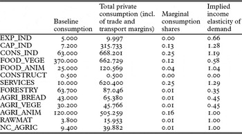
There are three income recipients in the model: a representative consumer, the government, and a fictitious agent called the investor. The representative consumer receives income in the form of factor rewards, net of income tax. It is assumed that a constant fraction of incomes is saved by the consumer. The remaining disposable income is used to buy goods. When income and prices change it is highly unlikely that the pattern of consumption stays unchanged. In other words, the income elasticity of demand differs between various types of good. To allow for such effects, I have modelled consumption by means of the Linear Expenditure System (LES) (Stone Reference Stone1954). In the LES, the consumption of a good consists of two parts. One part, which may be labelled the subsistence level of expenditure, stays the same irrespective of what happens to prices and/or income. The other part is proportional to the income that remains after the subsistence quantities have been bought and may also be viewed as the marginal propensity to consume a good.Footnote 16
In the model there is only one representative consumer; in other words, capitalists, workers and farmers are assumed to consume and save in exactly the same manner. That is obviously a gross oversimplification. If data had permitted it would have been preferable to have several separate income recipients, each with separate utility functions and savings rates. The latter typically varies a lot between different social classes; members of the working class save a tiny fraction of their income, while the bulk of savings derive from profits. In the real world changes in income distribution therefore affect the aggregate savings rate and thereby consumption. However, in the following static simulations the distribution between profits and wages typically changes by only 1–2 per cent of national income, so the failure to model differences in savings behaviour between social classes should not materially affect the results.
The government receives income by collecting taxes and uses this income to demand the output of the public services sector. The government is the only consumer of the output of the public services sector (PUBLICSERV). I have assumed that the level of government expenditures is exogenously given. If the government's income is larger than its outlay, which was the case in 1913 according to the benchmark SAM, the difference is saved.
Tariffs were an important source of revenue for the government. In 1913 tariffs accounted for about 25 per cent of total taxes. Of these, grain and food tariffs (excluding so called fiscal tariffs) made up roughly 25 per cent (in the model economy roughly one-third). If agricultural and food tariffs had been abolished, the government budget would turn from surplus to deficit if not compensated by other taxes. In the counterfactual simulations with the model I assume as part of a tariff reform package that income tax would rise endogenously to cover the eventual deficit resulting from diminishing tariff revenues.
The investor collects the savings of the representative consumer and the government. In addition, this agent also receives any capital inflow from the rest of the world and services foreign debt incurred in earlier periods. Since the value of imports generally exceeded export incomes, capital inflow was an important feature of Swedish economic development from the 1870s to World War I (Schön Reference Schön and Dahmén1989). The debts contracted in these decades resulted in contractual interest payments on the loans and accordingly an additional outflow of foreign exchange in addition to the current trade deficit. It was only in the years immediately preceding World War I that the Swedish trade balance started to turn positive. The debt service on foreign loans was only partly ameliorated by the money sent home to relatives by Swedish emigrants to the United States. This inflow of foreign exchange was nevertheless of some importance at the time and it is included in the endowment of foreign savings in the benchmark.
The investor uses the domestic and foreign savings he commands over to demand investment goods. There are no inventories in the model and hence no inventory investments. It is assumed that the volume of investment in fixed capital (machinery, equipment and buildings) is fixed, conceivably because it was ordered in a previous period. The model is closed by letting foreign savings adapt to ensure that total savings will always equal investments.
A CGE model solves for relative prices; one commodity must be assigned the role of a numeraire. For this purpose I use the price of foreign exchange, the exchange rate, which is set to unity. While the use of a numeraire does not affect relative prices in the model, and therefore not the results, certain aspects may be easier to elucidate depending on which numeraire is chosen. There is no monetary unit in a CGE model and hence the notion of a general price level is somewhat out of place since how nominal prices evolve is dependent on the chosen numeraire. However, in the real world with financial contracts and wage settlements expressed in money, the evolution of the general price level is obviously of great concern to the agents in an economy. In our period of interest Sweden was on the gold standard and accordingly used a fixed exchange rate. Expressing prices in the counterfactual simulations in terms of the price of foreign exchange seems to be the best way to mimic how nominal prices would have evolved in the real world.
Before we proceed to exercises with the model, some limitations of essentially static simulations should be mentioned. We explore the consequences of a tariff reform on the eve of World War I. We cannot from these simulations really tell what the Swedish economy would have looked like if agrarian and food tariffs had never been installed in 1888. Capitalists’ decisions to invest and workers' decisions to migrate or not, and thereby also the long-run evolution of factor endowments, would surely have been different if Sweden had followed a free trade policy, and technology might have been different too. A way to accommodate such long-run effects in CGE models is to simulate a sequence of equilibriums through time. In the period between the different equilibriums, endowments and possibly other exogenous variables are updated and then a new general equilibrium is solved and so on.Footnote 17 It is, however, very difficult to model the rate of investments, their sectoral composition and the rate of technical progress. More common seems to be to use CGE models in comparative static explorations. In these counterfactual scenarios it is typically assumed that capital is malleable, that it can be reshuffled between the sectors. In the present context this is tantamount to assuming that had the economy evolved without agrarian and food tariffs, capital goods with the same technical characteristics and with exactly the same total value as in the 1913 benchmark would have been accumulated; only their distribution among the various sectors would be different since capital owners would have had time to adjust their investments to the pattern of demand in a Swedish economy without food tariffs. The idea seems to be that by making this thought experiment of complete capital mobility, static counterfactual simulations tell us something about the long-run effects of tariffs. As will be seen in the following counterfactual simulations, we obtain about the same income-distributional impact of agrarian tariffs whether we assume fixity of capital in each sector or full capital mobility. In each simulation the model has been solved using the GAMS/MPSGE software.
5. What would have happened if agrarian tariffs had been removed? Counterfactual simulations
5.1. Preliminary remarks on data
To better interpret the counterfactual scenarios reported in this section it is useful to first make a few remarks about the data and elasticities used in the model. The input–output table of the Swedish economy in 1913 (Appendix 2, Table A2.6) and the final demand table (Appendix 2, Table A2.1) clearly show that the main outlet for the products of the agricultural sector was the food industry; the AGRI_BREAD sector provided the FOOD_VEGE sector with inputs and the AGRI_ANIM sector supplied the FOOD_ANIM sector. The forward linkages from the agricultural sectors to other sectors were of little importance. As a consequence, the other sectors would be little affected by a withdrawal of agrarian and food tariffs, except through changes in wages and labour availability. It should also be noted that the AGRI_VEGE sector is essentially an adjunct to the AGRI_ANIM sector. Most of its output was delivered to the AGRI_ANIM sector and the two sectors might as well have been aggregated to one sector.
A special problem in calibrating the model is the choice of elasticities. There is admittedly not much empirical basis for deciding on the various elasticities that are used in the model. There seem to be three approaches in the literature: own econometric estimates, use of estimates obtained from other studies, and more or less educated guess work.
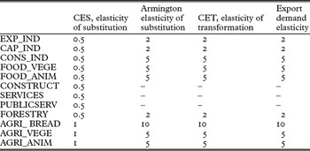
There is a large econometric literature on CES production functions. However, it has been shown that estimates of substitution elasticities are much dependent on the chosen specification (Heathfield and Wibe Reference Heathfield and Wibe1987, ch. 9). According to an estimate by Jungenfelt (Reference Jungenfelt1966), the elasticity of substitution in Swedish manufacturing was 0.6 in 1870–1950. Jungenfelt's estimate seems to have been accepted in other CGE models for Sweden (Karlström Reference Karlström1985; O'Rourke and Williamson Reference O'Rourke and Williamson1995; Vikström Reference Vikström2000), and an elasticity of substitution of about 0.5–0.6 for the manufacturing industry also appears to be standard in CGE modelling (Federico and O'Rourke Reference Federico, O'Rourke, Pamuk and Williamson2000). I have therefore decided on an elasticity of substitution of 0.5 in the CES production functions for all but the agricultural sectors where the elasticity is set to unity, as seems to be common in many CGE applications, the argument being that if there is any activity where substitution between the factors of production is feasible to any extent it is within agriculture.
There have also been many attempts to estimate Armington elasticities econometrically, but these typically refer to more recent data. Moreover, it has been shown that such estimates are very sensitive to the level of aggregation and the frequency of the data; more disaggregated data yield higher estimates and high-frequency data generally yield lower estimates than low-frequency data (McDaniel and Balistreri Reference McDaniel and Balistreri2003). In the absence of econometrically well-founded estimates I have used figures for Armington elasticities similar to the ones used in other CGE models. It is reasonable to assume that the elasticity of the world supply curve facing Swedish grain consumers was high, so that the percentage change in the import penetration ratio would have been quite large as a result of a dismantling of bread-grain tariffs. With this argument, I have set the Armington elasticity to ten for the bread-grain sector. It seems likely that the Armington elasticity was lower for processed food products than for bread-grain, because of varying national tastes. I have therefore decided on an Armington elasticity of five in the FOOD_VEGE and the FOOD_ANIM sectors. Partly based on own estimates on trade data, I have also set the Armington elasticity for the consumer goods industry, the CONS_IND sector, to five while it is set to two in the remaining sectors.
The empirical basis for deciding on export price elasticities and CET transformation elasticities is even weaker than is the case for Armington elasticities and CES substitution elasticities. It seems to be standard practice in CGE models to set high numbers on CET transformation elasticities.Footnote 18 I have followed this practice for agricultural goods and have simply used the same numbers for the export demand and CET elasticities as for the Armington elasticities.
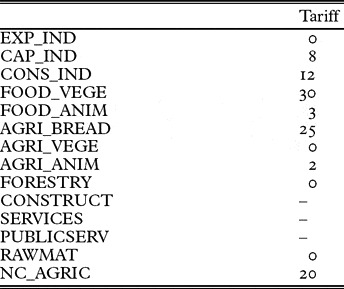
In the following three counterfactual simulations, we look at what happens in the model when we remove all agricultural tariffs and the tariffs protecting the food industries. The sales tax on the output value of the FOOD_VEGE sector is also removed, but tariffs on NC_AGRIC imports are kept.
5.2. Simulation 1: sector-specific capital in all sectors, no labour mobility between urban and rural labour markets
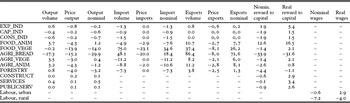
In this simulation, land and farm capital is specific to each sector of agricultural produce, that is, land used for growing bread-grain cannot be used for pasture or for growing other arable products. The result from this simulation is reported in Table 9. The most obvious effect is that prices fall steeply for bread-grain producers. Import prices are reduced by 20 per cent resulting in a rise of import volumes by almost 50 per cent. Bread-grain output contracts since labour inputs are reduced. The revenues of bread-grain producers fall by 30 per cent, primarily as a result of falling sales prices. As a result, the factor rewards for owners of bread-grain farms take a dive of more than 30 per cent.
Simulation 1: sector-specific capital in all sectors, separate urban and rural labour markets. Percentage changes in output and prices

The labour released from the bread-grain sector is employed in other agricultural sectors, leading to a slight increase (about 3 per cent) in their output, which is sold at prices reduced by roughly the same amount. On balance the AGRI_VEGE and the AGRI_ANIM sectors are little affected by the tariff reform package. The reward to capital in these sectors only declines slightly in nominal terms, but when deflated by a consumer price index,Footnote 19 which falls by 3.4 per cent, buying power of profits rises so that in real terms the rewards to farm owners in these sectors increase.
Post-tax nominal wages for rural workers declines by 7.2 per cent. Because of increased imports of bread-grain the demand curve for labour shifts inwards in the agricultural sectors. Since full employment of rural labour is assumed, the labour supply curve is infinitely inelastic and the inward shift of the labour demand curve leads to a commensurate decline in nominal wages. In the urban sectors, nominal wages decline by 0.6 per cent. However, both rural and urban labour benefit from lower prices on consumer goods. Hence post-tax real wages for rural workers fall by 4 per cent, while they rise for urban workers by 2.9 per cent. To prevent the government budget from falling into deficit as a result of declining tariff revenues, income tax is raised by 1.1 percentage units to 5.8 per cent.Footnote 20
In real terms, in other words, profits deflated by a consumer price index, the reward to capital owners in non-food urban industries increases. They benefit from falling nominal wages while their own output prices only fall slightly. Of particular interest is what happens to the food industries. The output of the animal food industry (FOOD_ANIM) increases more than prices are reduced. With declining nominal wages and falling input prices this leads to an increase in the rewards to capital owners by more than 15 per cent in real terms. The vegetable food industry (FOOD_VEGE), on the other hand, faces harder competition from imports. The import volume increases by 75 per cent and sales prices in this sector fall by almost 15 per cent, but the output volume is only slightly altered. The reward to capital owners only falls slightly in nominal terms, and even rises by 2 per cent in real terms. Apparently, falling input prices and nominal wages were enough compensation for falling output prices.
5.3. Simulation 2: sector-specific capital in urban sectors, common factor ‘land’ in agrarian sectors, no labour mobility between urban and rural labour markets
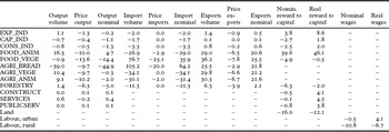
In this simulation, the results of which are reported in Table 10, I drop the assumption that land used for growing bread-grain is confined to producing these crops. Surely the owners of this land could convert their wheat fields and rye fields to pasture or to the growing of oats and green fodder of various sorts. To increase their stock of animals would take time and incur investment costs, but in this simulation we ignore these facts of the real world and envisage that their farm capital could somehow be effortlessly remoulded (fewer wheat fields, more pasture and livestock). Thus, in the simulation reported in this section I assume that ‘land’ can be used equally well for producing milk as for producing wheat or other crops, so that in all agricultural sectors the primary factors are land and labour. I keep the assumption that there are two labour markets: one for rural and one for urban workers with no labour mobility between them.
Simulation 2: sector-specific capital in urban sectors, common factor ‘land’ in agrarian sectors, separate urban and rural labour markets. Percentage changes in output and prices

The most obvious change following a tariff reform is that bread-grain output falls by 39 per cent and prices by 10 per cent. As a result, sales revenues fall by more than 40 per cent. The reason behind the contraction in bread-grain output is of course increased competition from imports. According to the simulation, the volume of bread-grain imports increases by 105 per cent. Bread-grain landowners, pressed by competition from imports, switch over to other crops (AGRI_VEGE) and to animal produce (AGRI_ANIM), which raises output in these sectors. In order for the increased output to be absorbed by the market, prices would have to fall at approximately the same rate, leaving nominal output only slightly changed. All in all, the rewards to landownership fall by 17 per cent in nominal terms or 13 per cent in real terms as a result of the tariff reform.
Imports of vegetable food products increase by more than 75 per cent. The percentage change in imports is large also in the other agricultural and food-producing sectors, but the initial import levels were quite low (see Appendix 2, Table A2.1) so a high percentage rate of change only generates small level changes. Exports from the agricultural and food-producing sectors are affected by a tariff reform, but among these sectors only the animal food industry (FOOD_ANIM) had any sizable export from the beginning. Thus the 29 per cent increase in the export volume of the FOOD_ANIM sector generates more export income than the combined increase in exports of the other sectors. The output of the vegetable food industry does not change much, but sales prices decline by almost 15 per cent, leading to a decline of sales revenues at approximately the same rate. Prices fall also in the animal food industry (by 8 per cent), but output increases more (by 16 per cent), leading to increased sales revenues.
The reward to capital owners in the animal food industry rises by a staggering 46 per centFootnote 21 in real terms, while it stays basically unaffected in the FOOD_VEGE sector. Value-added shares were low in the food-producing industries, particularly in the animal food industry, hence falling input prices weigh much heavier in their costs than changes in the wage rate.
The factor rewards to owners of capital in non-food-producing urban sectors generally improve in real terms, particularly in the export industry, since its most important input, emanating from the forestry sector, falls in price, because of the fall in rural wages.
Rural wages net of income taxFootnote 22 decline by 11 per cent while urban wages stay largely unaffected. Of interest for workers would have been not only how money wages developed. Above all, they would have been interested in what they could buy for their wages. The consumer price index declines by 4.4 per cent, so that post-tax real wages in the urban sectors rise by 4.1 per cent, while those of rural workers decline by 6.7 per cent.
5.4. Simulation 3: sector-specific capital in urban sectors, common factor ‘land’ in agrarian sectors, labour mobility between urban and rural labour markets
In this simulation I release the assumption of no connection between the labour markets for urban and rural workers and assume instead that there is labour mobility between the urban and rural sectors. This is the only change compared to simulation 2. I still maintain the assumption that there were persistent wage differences between the various sectors for each labour category caused by a ‘wage distortion’ factor.
To model rural–urban labour mobility I use a fictitious sector ‘producing’ rural and urban labour with ‘raw labour’ as input. In the benchmark the output of rural and urban labour is the same as was factually the case in 1913 (see Table A2.2). When the rural–urban wage differential changes, there is a concomitant change in the output of rural and urban labour. In other words, labour moves between the urban and rural labour market in response to changes in relative wages. How much labour mobility reacts to a change in relative wages, or in model technical terms how much rural and urban labour is ‘produced’, is modelled by a Constant Elasticity of Transformation function.Footnote 23 The extent of rural–urban labour migration, and therefore also how much the rural–urban wage differential is affected by it, is dependent on the chosen CET elasticity, which roughly tells by how many percentage units the urban–rural employment ratio changes in response to a percentage change in the urban–rural wage ratio. If, for example, the CET elasticity is set to unity, a 5 per cent increase in the urban–rural wage ratio would lead to a 5 per cent increase in the urban–rural employment ratio. In other words, a high CET elasticity means that rural–urban migration responds strongly if the relative gap between urban and rural wages widens, which in its turn prevents the gap widening as much as it would in the absence of labour mobility.
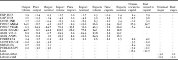
In the following simulation, the results of which are reported in Table 11, I assume a CET elasticity of 5. That is probably an unrealistically high figure,Footnote 24 but it has the advantage of illustrating the importance of labour mobility for the level of urban and rural wages. When allowing for such a high degree of labour mobility between the urban and rural labour markets, nominal post-tax wages for urban workers fall by 5 per cent following a withdrawal of agricultural and food tariffs. Rural workers moving to the urban sectors put a downward pressure on wages and the income tax rate increases from 4.7 per cent to 5.7 per cent to compensate for falling tariff revenues. In this simulation the consumer price index falls by 5.1 per cent, so that urban real wages stay largely unaffected. With less competition for jobs in the rural labour market, the lot of rural workers is improved compared to the earlier simulations which did not allow for rural–urban labour mobility; rural post-tax wages fall by 6 per cent in nominal terms or by 1 per cent in real terms.Footnote 25 A lower degree of rural–urban labour mobility would obviously be beneficial for urban workers. If we lower the CET elasticity to 0.5, urban real wages increase by 2 per cent and rural real wages decline by 3.8 per cent, while an elasticity of unity leads to a rise in urban real wages of 1.3 per cent and a fall in rural real wages by 2.7 per cent.
Simulation 3: sector-specific capital in urban sectors, common factor ‘land’ in agrarian sectors, one labour market. Percentage changes in output and prices

It may be argued that nominal wages were not fully flexible downwards and that therefore the assumption of full employment is unwarranted. In another simulation I experimented with letting nominal wages be completely inflexible downwards; in other words, they are not allowed to fall below the benchmark level. In this case, with a transformation elasticity of 5, unemployment rises to about 5 per cent after a dismantling of agricultural and food tariffs, while obviously those workers who keep their jobs benefit from lower prices, leading to improved real wage rates for both urban and rural workers.
The reward to landowners falls by about as much as in the previous simulation. The real beneficiaries of rural–urban labour mobility are urban capitalists. In real terms, urban capitalists would generally gain a lot from cheapened labour costs when supply increases in the urban labour market, following labour migration from the rural sectors. How much capital owners gain may be readily seen if we assume that capital moves between the urban sectors so that profit rates are equalized.Footnote 26 In that case the real reward to capital owners (the return to capital deflated by a consumer price index) would increase by 3.9 per cent compared to the benchmark with tariffs. This is about the same figure that we get if we calculate the weighted average of real rates of return to capital in Table 11, using each sector's benchmark share of the total value of capital as weights (see Table A2.2). In general, the results of a simulation with mobile capital change very little compared to Table 11.
5.5. General discussion of the simulation results: winners and losers of agrarian protectionism
A CGE model is based on some quite restrictive assumptions. While obviously the exact figures of the counterfactual simulations should be taken cum grano salis, they should be able to produce reasonable numbers on key parameters and a few general conclusions seem possible. Before discussing the income-distributional impact of agrarian and food tariffs, some other results from the simulations should be mentioned.
One effect of protectionism was that it tended to raise the general price level. According to the simulations, consumer prices fall by about 5 per cent in terms of the price of foreign exchange after a withdrawal of agricultural and food tariffs. It is also possible to calculate the change in the GDP-deflator in the counterfactual simulations. It falls 1–2 percentage units less than the consumer price index. With fixed exchange rates, as was the case under the gold standard, a fall in the general price level makes the service of foreign loans dearer in real terms. Moreover, a fall in the general price level would affect the position of creditors and debtors generally in the economy, but these effects are not taken into account in the model simulations, where there are no financial assets except foreign loans.
In the late nineteenth and early twentieth centuries, tariffs were not only an important industrial policy measure, but also an important source of revenue for the government. Important for the simulations results is that income tax rises by about 1 per cent of factor incomes to compensate the government for falling tariff revenues. Thereby a distortionary tax (agricultural and food tariffs) is substituted by a non-distortionary tax (a general income tax).Footnote 27 The effect of the tax reform on real GDP is marginal. It only changes by a tiny fraction of a percentage unit in the simulations, which is unsurprising since technology and endowments remain unchanged throughout the simulations. Nevertheless general welfare rises since price declines on consumer goods improve the real income of the representative consumer, measured in terms of the benchmark consumption basket, by about half a per cent or slightly more. The static welfare gain of a tax reform is small; its main effects would be on income distribution not the level of income.
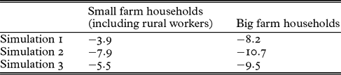
Those who benefited most from agrarian protectionism were obviously farmers specializing in bread-grain production. They would unequivocally lose a lot from a removal of agrarian tariffs. What would have happened to farmers specializing in animal produce depends on the extent to which producers in the bread-grain sector were able to switch over to animal husbandry. If we disregard transition costs, output of animal products would expand at the expense of bread-grain. The reward to landownership would in this case fall by roughly 10–15 per cent in real terms (simulations 2 and 3). This figure should be interpreted as what the average landowner would lose from the dismantling of agrarian and food tariffs given the opportunity to switch over from bread-grain to animal produce. Small farmers would in general fare better since most of them already specialized in animal husbandry, but they would still lose since even if small farms specialized heavily in animal produce they also produced some bread-grain. Moreover, small farmers were also dependent on wage income for their livelihood, whether on imputed wages for labour they performed on their own farms or wages for part-time labour on larger estates. Some back-of-the-envelope calculations may suggest the approximate numbers involved. If we define farms up to sizes of 10 hectares as ‘small’, their share of output in the various agricultural sectors can be seen from Table 5 above. If we further assume, based on Höijer (Reference Höijer1921c, p. 52), that 85 per cent of the agricultural labour force was employed in small farms, or as non-family employees in ‘big farms’,Footnote 28 we may calculate the effects of agrarian tariffs on the real income of households of small farm owners and landless rural workers on the one hand and big farm households on the other. The results are displayed in Table 12. The most advantageous simulation for households of small farmers and rural workers is simulation 1, where real reward to capital in animal produce slightly rises. In this simulation, real incomes of small farm households fall by about 4 per cent compared to the benchmark, while they fall by 8 per cent for big farm households.
Percentage change in real incomes in counterfactual simulations compared with benchmark. ‘Small farm’ households (including rural workers) and ‘big farm’ households
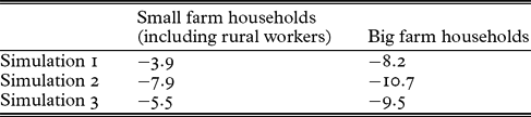
Table 12 probably overstates the losses that households of small farmers and rural workers would incur after a tariff reform since the consumer price indexes used to deflate nominal incomes in the simulations understate the price decline in the consumer basket of rural workers and small farmers. Those households had incomes much below the average and should therefore have consumed proportionally more food products, especially vegetable food products. Given figures on the total consumption outlay of rural workers and small farmers and income elasticities of demand, we may calculate the share of the various goods in their 1913 consumption basket and thereby how much its price would have fallen in the various simulations.Footnote 29 It falls by roughly 2 percentage units more than the price index of the representative consumer, mainly because vegetable food products account for a third or slightly more in the consumption basket, compared to slightly below 25 per cent for the representative consumer. Falling food prices would have cheapened consumption more for rural workers and small farmers than for urban workers. Still their income would have fallen more than prices for the goods they bought. The results of the counterfactual simulations underline what can be shown by effective protection rates; namely that small farmers gained from agrarian protectionism, although not at all to the same extent as large landowners.
After removing agrarian tariffs, nominal wages of rural workers would generally fall more than prices of consumer goods, leading to falling real wages. What would have happened to urban workers depends on the extent to which the rural and urban labour markets were integrated. If the two labour markets were insulated from each other, money wages of urban workers would be little affected and they would enjoy increasing real wages because of falling food prices. If we allow for labour mobility between rural and urban labour markets, the real wage gains of urban workers resulting from falling food prices would be less certain. The gain of urban workers from a tariff reform is dependent on the extent of rural–urban labour migration. If labour migration responds strongly to a change in the urban–rural wage differential, the gains of the urban workers from a tariff reform might even vanish. However, reasonable assumptions regarding the extent of rural–urban labour migration lead to the conclusion that urban workers would gain from a withdrawal of agricultural and food tariffs.
Capital owners in non-food urban industries would generally gain from a dismantling of agricultural and food tariffs, on average by 3–4 per cent in the simulations. Since there were hardly any backward linkages from these industries to agriculture, they would primarily be affected by changes in product wages, tax payments and final demand for their products following a tariff reform. For most of these industries the most favourable of our simulations is the one with extensive migration between the urban and rural labour markets when nominal wages would decline in urban industries following increased labour supply.
Of special interest for the issues in this article is how capital owners in the food industries would be affected. In the simulations the reward to capital owners in the animal food industry increases considerably, since output increases as a result of enlarged exports while input costs decline. Their peers in the vegetable food industry would only lose slightly or not at all as in the first simulation, despite sharply falling sales prices. Apparently, lower nominal wages and input prices compensate for falling output prices.
The results may be put in perspective by comparing them with O'Rourke's CGE model for Sweden calibrated with data from 1871 (O'Rourke Reference O'Rourke1997, p. 792, table 7). O'Rourke assumed a high degree of rural–urban labour mobility so his results should be compared with simulation 3 in this article. My 1913 model calibrated with data from 1913 differs in a number of aspects from O'Rourke's; for example, there were no bread-grain tariffs in the 1870s and accordingly no need to model compensatory increases in other taxes to substitute for withdrawn tariffs. He also assumed a larger price shock in his counterfactual simulations in line with the fall in wheat prices following the ‘grain invasion’ in the 1870s. Above all, the structure of the economy had changed considerably between 1871 and 1913. Animal husbandry was much more important in 1913 and employment in agriculture as a share of total employment had declined from almost 70 per cent to less than 45 per cent (Jungenfelt Reference Jungenfelt1966, pp. 224–9). These changes make understandable the differences in simulation results. Reward to landownership declines somewhat less in my 1913 model, which is natural given the substantial decline in the share of bread-grain of agrarian output between 1871 and 1913. Another difference is that the profitability of capital owners in urban industries benefited more from a fall in agrarian prices in O'Rourke's 1871 model. This is also explainable by the change in economic structure, since the influx of rural labour to urban industries would have been relatively less important in 1913, generating a smaller rate of increase in labour supply in urban industries, which now occupied a much larger share of the economy than in the 1870s.
6. Conclusion
The invasion of cheap overseas grain in the 1880s provoked the reintroduction of grain tariffs in Sweden as in many other countries on the European continent. Agrarian protectionism was filled with controversy from the beginning. Tariffs were high on bread-grain while oats, the most important crop for the majority of farmers, were left unprotected. Protection of animal products was low or non-existent. Despite high protection of bread-grain its share of output declined while the output of animal produce increased strongly. Agricultural protectionism slowed down this process somewhat, but did not alter its general course. Small farmers in particular specialized in animal produce, and they had consequently less to gain from agricultural protectionism than larger farms.
Counterfactual simulations with a computable general equilibrium model of the Swedish economy calibrated with data from 1913 suggest that on average agrarian protectionism raised the reward to landownership by 10–15 per cent in real terms. Real income of households of small farmers and rural labourers would have fallen by about half of that amount, or slightly less, if agrarian tariffs had been abolished. Even though they specialized in animal output, small farmers also produced some bread-grain, and they also derived income from rural labour for which real wages would have declined if agrarian protectionism had been dismantled.
As economic theory predicts, there would also have been gainers from a tariff reform. Simulations suggest that profits of urban capitalists would have increased by 3–4 per cent in real terms. Given reasonable assumptions on rural–urban labour mobility, urban labour would also have gained since money wages would have declined less than prices of consumer goods, leading to real wage increases of 2–4 per cent.
Economic development in the preceding centuries had made the agricultural sector less sensitive to a price shock of the sort that would have followed upon a withdrawal of agrarian and food tariffs. Still, the benefits and burdens of adjustments would have been unequally shared by different social classes and strata, which made the proposals for a tariff reform controversial. The article illustrates a general theme in the literature on the political economy of tariffs. There was one group that clearly benefited from agrarian protectionism, namely predominantly large landowners specializing in bread-grain production. The eventual benefit to other groups in society of a dismantling of agrarian protectionism was smaller and less clear-cut. This also explains why agrarian protectionism, though controversial, showed great persistency once instituted.
Acknowledgements
The research for this article was supported by a grant from Stiftelsen Riksbankens jubileumsfond. I have benefited from comments by participants at the Sixth Conference of the European Historical Economics Society in Istanbul 2005 and at the Economic History Seminar at the Department of Economic History, Gothenburg University, where earlier versions of the article were presented. Carl-Johan Gadd and Martti Rantanen have educated me on some aspects of late nineteenth-century Swedish agriculture, while Svante Prado made many suggestions of a more general character on different versions of the article. The article was also improved by critical comments from two anonymous referees. As always, I take full responsibility for all remaining errors.
Appendix 1: Sources and methods used for calculating farm output, labour use and effective protection rates at farms in different size-classes
A1.1. Farm output
For the year 1919, we have data on the number of farms and hectares cultivated by farmers in the following size-classes: 0–0.25 hectares, 0.25–2 hectares, 2–5 hectares, 5–10 hectares, 10–20 hectares, 20–30 hectares, 30–50 hectares, 50–100 hectares, larger than 100 hectares (Höijer Reference Höijer1921b, pp. 64–5, table 14). From the same source, we also have information for the different size-classes of farms on how large a share of the acreage was used for fallow and for the growing of various crops (Höijer Reference Höijer1921b, p. 90, table 17a). In addition, there are data for the same size-classes of farms on output (harvest and seed) for wheat, rye, barley, oats, peas and beans (Höijer Reference Höijer1921c, pp. 54–74, table 51). For other crops, I have assumed that the output and seeds for each crop on each farm were the same per hectare as the national average. In order to calculate output for the various crops per classes of farm size, I have assumed that their shares of output in 1913, as given by Lindahl et al. (Reference Lindahl, Dahlgren and Kock1937, pp. 30–48, table 66), were the same as the corresponding shares in 1919.
From Historical National Income statistics, we have estimates for each year on the number of animals (horses, bullocks, bulls, cows, young cattle and calves, sheep, goats, pigs and poultry) (Lindahl et al. Reference Lindahl, Dahlgren and Kock1937, pp. 92–8, table 69). To estimate the number of animals for different farm sizes in 1913, I have assumed that the size distribution for the various animals was the same as in 1919. For the latter year, we have information for each size-class of farms on the number of horses, cows, young cattle and calves, bullocks, bulls, pigs, goats, sheep and lambs (Höijer Reference Höijer1921b, p. 102, table 23a–b). For poultry, we lack information on the size distribution of the number of animals. Poultry was more common among small farmers. To make an educated guess on the distribution of hens among farms of different sizes I have used information (Höijer Reference Höijer1919, pp. 246–64, tables 1–2), which gives data on the number of hens per size-class in 27 härads (an administrative unit) in southern and central Sweden for the year 1917. To estimate the output of animal food products on the various size farms in 1913, I have simply assumed that the output per animal of meat, milk, eggs and so on was the same as the national average according to historical national accounts (Lindahl et al. Reference Lindahl, Dahlgren and Kock1937, pp. 92–8, table 69; p. 111, table 73b; p. 117, table 74; pp. 30–1, table 75).
Output of the various crop products and animal products has been valued at prices given by Lindahl et al. (Reference Lindahl, Dahlgren and Kock1937, pp. 53–4, table 68; pp. 110–11, table 73a–b).
A1.2. Labour use
To calculate the labour input in the various parts of arable and animal husbandry, I have used estimates of normal labour use in different agricultural activities provided by Nanneson (Reference Nanneson1922).Footnote 30 Accordingly, it is assumed that the work hours per hectare and animal in each line of production were the same for each farm size.
A1.3. Calculations of effective protection rates
In order to calculate effective tariffs, we need data on nominal tariffsFootnote 31 and cost shares for inputs. I have assumed that fertilizer was the only purchased input in the production of grain and other crop products.Footnote 32 I have made an educated guess on the cost shares of fertilizer from material presented by Nanneson (Reference Nanneson1916, pp. 30–3, 62–6). It is assumed that the use of fertilizer per hectare and crop was the same in each size-class of farms.
The only purchased input in animal production is concentrated fodder. Based on data given by Nanneson (Reference Nanneson1916, pp. 57–62), I assume that the cost share of concentrated fodder (mainly hay, oats and oil-seed cakes, all of which were duty-free) was 40 per cent of the sales value of live cattle in 1911/14.
For hog production, I have assumed that the cost share of purchased inputs in the sales value of hogs was 70 per cent in 1911/14 and that maize accounted for 85 per cent of these inputs. Poultry output was largely concentrated in small farms, and chickens and hens were to a large extent fed by leftovers from the farm households. For simplicity, I have assumed in the calculation of effective protection rates that no purchased inputs were used in poultry production.
Assuming the same physical input–output relationships for other years, the cost shares of purchased inputs for 1901/5 and 1906/10 have been calculated on the basis of price data given by Ljungberg (Reference Ljungberg1990) and Swedish foreign trade statistics.
Appendix 2: Benchmark data for the CGE model
Income and sales taxes
The tax system at the time was a complicated mixture of taxes of various sorts. For simplicity, I assume that all factor owners pay an income tax amounting to 4.7 per cent of their income. This rate conforms fairly well to total state and municipal income taxes in 1913 (Gårestad Reference Gårestad1987, pp. 196–7, table 1). If data had permitted it would have been preferable to make a distinction between income tax on wages and other factor incomes. The income tax rate for workers was lower than for other income categories and some workers with low income paid no income tax at all. Another important source of revenues for the government was indirect taxes. Sales taxes were levied on liquor, sugar and beer (Gårestad Reference Gårestad1987, pp. 208–9, table 3). I assume that the FOOD_VEGE sector paid 5 per cent of sales revenues in sales tax.
Final demand and supply, 1913 m kr

Sources: See Table A2.5.
Notes:
aIndustrial and agricultural goods were not sold directly to the final consumer. They were processed by the retail trade sector before final consumption. In line with Swedish Historical National Accounts (Krantz Reference Krantz1991), I have assumed that those goods were marked up by the SERVICES sector by a given percentage on the sales value. Of the consumption figure for the SERVICES sector, 596.7 m kr was consumption of retail services. Accordingly, the margin of transport and trade services on final consumption goods was 30.8 per cent.
bExports from the private services and transport sector (SERVICES) resulted from commercial margins on commodity exports from other sectors and from shipping the export goods to foreign ports. Exports from this sector should be viewed as input to final exports. Accordingly, exports from the other sectors valued ex factory are marked up by 31.6 per cent by exports from the SERVICES sector to arrive at final exports.
Factor payments and capital stock (1913 m kr). Employment (1000s)

Sources: Appendix 1; Flodström Reference Flodström1912; Jungenfelt Reference Jungenfelt1966; Schön Reference Schön1988; Sveriges officiella statistik. Industri, 1913; SOU 1923:37.
Note: Employment in the manufacturing industry is derived from Swedish industrial statistics (Sveriges officiella statistik, Industri, 1913). The employment figures also include employees in small firms and handicrafts not included in the industrial statistics, derived from Schön (Reference Schön1988, pp. 109–15, table 14). For data on total employment in the agricultural sector (including forestry and fishing), see Jungenfelt (1966, pp. 224–9, table 1). The estimation of employment in each of the agricultural sectors is described in Appendix 1. The number of employees in the forestry sector is an educated guess based on the total number of employees in agriculture (including forestry and fishing) according to Jungenfelt and estimates of agricultural employment in Appendix 1, above. Data on employment in other sectors also derive from Jungenfelt.
To calculate wage sums we also need data on wage rates. For the manufacturing sectors these derive from wage sum data (SOU 1923:37) and data on employment and sales values from the industrial statistics (Sveriges officiella statistik, Industri, 1913). Wage data from the other sectors derive from Jungenfelt.
Capital stock data for the manufacturing sectors derive from a public investigation on costs in the manufacturing industry in 1913 (SOU 1923:37). For the other sectors they are based on 1908 data presented by Flodström (Reference Flodström1912). Flodström's 1908 figures have been marked up by 10 per cent to arrive at data for 1913. It should be noted that capital stocks data are only needed for the calculation of depreciation rates; otherwise they are not needed for calibration of the CGE model. For this we only need income shares of labour and capital.
Consumption data for formulation of Stone-Geary utility function, 1913 m. kr

Note: Baseline consumption levels have been calculated by means of own econometric estimates which have been hand adjusted to make them internally consistent. The income elasticity of demand for a good is calculated as the marginal consumption share divided by the total private consumption share of that good.
Elasticities used in counterfactual simulations

Benchmark tariffs on imports (%)

Savings
The difference between post-tax factor incomes, after deduction of depreciation on fixed capital,Footnote 33 and the value of total private consumption is saved. Accordingly, the savings rate of the representative consumer is computed as (Factor incomes – income tax – depreciations – total private consumption)/ (Factor incomes – income tax – depreciations). This savings rate is applied in all counterfactual simulations. Government savings equal the difference between the sum of all taxes (tariffs, income and sales taxes) and the governments purchase of PUBLICSERV output, which is fixed. In the counterfactual simulations income tax adapts to ensure that the government will not incur debts as a result of the removal of agricultural and food tariffs. Government savings, private savings and depreciations are transferred to ‘the Investor’.
Apart from domestic savings the Investor also receives or transfers foreign exchange to the outside world. I have assumed that the rate of interest on the stock of foreign debt was 3 per cent, which was paid on a foreign debt of 2,660 m kr in 1913. This results in a ‘negative endowment’ of foreign exchange in the benchmark amounting to 79.8 m kr. There is also an inflow of emigrant remittances amounting to 36 m kr. according to the estimates by (Lindahl et al. Reference Lindahl, Dahlgren and Kock1937, pp. 598–9, table 174).The difference between imports (exclusive of tariffs) and exports is filled by foreign savings. Hence foreign savings in the benchmark is: imports – exports – emigrant remittances + interest payment on foreign debt. In the counterfactual simulations foreign savings adapt to ensure that total investments equal total savings.
Input–output table of the Swedish economy 1913, m kr

Sources: See input–output table for the Swedish economy in Bohlin (Reference Bohlin2007) and the sources cited therein.