1 Introduction
When modeling data in supervised learning, we most commonly evaluate induced predictive models by computing the accuracy measures that are averaged across all testing examples. Such averaged accuracy measures are, for example, the mean squared error (MSE) and the relative mean squared error (RMSE), which summarize the error contributions of test examples but do not provide any information about the expected error of a particular unseen example. In modeling efforts, which include achieving the best possible prediction accuracy for the unseen examples that were not included in the learning process (Kononenko & Kukar, Reference Kononenko and Kukar2007), we might find such information about single prediction reliability (Crowder et al., Reference Crowder, Kimber, Smith and Sweeting1991) important and beneficial.
Important potential application areas of the individual prediction reliability estimates are the risk-sensitive applications of machine learning (e.g. medicine, financial, control applications, and so on). Namely, the availability of additional information about prediction reliability can enable users of the decision-making applications to decide to what degree they can trust the prediction. The physicians, managers, operators, and so on can therefore use the reliability estimates to decide whether they will accept the system’s prediction and perform a corresponding action in the real-world (e.g. prescribe a medicine, make a business decision, change navigation direction, and so on) or not. In contrast to the averaged accuracy measures, which allow the user to evaluate the model’s accuracy (induced on a given set of training examples) on the whole, the individual prediction reliability estimates, therefore, allow users to perform accuracy evaluation on an example basis.
Besides providing reliability information, the concept of estimating individual predictions reliabilities has also an advantage to the averaged accuracy measures. Since this approach, in contrast to the averaged accuracy measures, does not require test examples and knowledge of their true labels, the reliability estimates can be computed for an arbitrary unseen example. This advantage is illustrated in Figure 1, which shows a contrast between the average reliability estimate (e.g. MSE) and the reliability estimates of individual predictions.
Reliability estimate for the whole regression model (a) in contrast to reliability estimates for individual predictions (b)

At a glance, in contrast to the averaged accuracy measures, which accurately express prediction accuracy for some test set, the task of predicting reliability for yet unseen examples poses as harder. The success of individual prediction reliability estimation (Figure 1b) indeed mostly depends on the design of such methods. To tackle this challenge, the related work in this area included the development of various methods. Basically, we can divide these methods into two families, with respect to how they are bound to the underlying prediction model. These two families are: (i) model-dependent approaches and (ii) model-independent approaches. The first group of approaches is focused on extending formalizations of specific classification and regression models, hence upgrading them to output reliability estimates as a supplemental information to the predictions. Due to exact model-related formalizations, these approaches are able to exploit the model-specific properties and can, therefore, be defined with the probabilistic interpretation (meaning that the estimate’s values belong to the interval [0,1], where 0 represents the confidence of the most inaccurate prediction and 1 the confidence of the most accurate one).
In contrast, the model-independent approaches are more general and utilize the predictive models as their parameters (black box principle). The approaches from this group are mostly based on estimating the reliability of the individual examples by observing the local influence of a particular learning example to a model, either by influencing the parameters, which are available in any supervised learning framework (e.g. the learning set, attributes, and so on), local modeling or by exploiting general properties of the input space. Since the formalizations of these approaches do not depend on models’ formalizations, they are harder to evaluate analytically with the individual models. The reliability estimates that are based on these approaches are, therefore, usually not probabilistically interpretable, meaning that they can take values from an arbitrary interval of numbers.
Our previous work (Bosnić & Kononenko, Reference Bosnić and Kononenko2007, Reference Bosnić and Kononenko2008b) aimed at developing general, model-independent approaches, which can be used to estimate prediction reliability of the arbitrary regression model. We proposed and compared nine model-independent reliability estimates (their basic versions and their variants) that were based on various approaches: sensitivity analysis, measuring variance of bagged predictors, local cross-validation, density-based estimation and local error estimation. The testing results of individual reliability estimates, achieved by measuring the correlation of the reliability estimates to the prediction error, showed that the estimates have a potential for estimation of the prediction reliability. However, although using model-independent reliability estimates, the results showed that different estimates achieve different performance on different domains and with different regression models. This issue left an open challenge to design an approach for the automatic selection of the reliability estimate that would perform best (i.e. to achieve best correlation with the prediction error among all available estimates) for the given domain and the given model.
In this paper, we propose and test two approaches to automatic selection of the best performing reliability estimate for a given problem domain and regression model: internal cross-validation and meta-learning. The paper is organized as follows. Section 2 summarizes previous work from related areas of individual prediction reliability estimation and Section 3 summarizes the reliability estimates that we use in the proposed approaches for automatic reliability estimate selection. We describe our testing environment and the testing protocol in Section 4. Sections 5 and 6 define and evaluate the proposed two approaches for automatic reliability estimate selection. In Section 7, we describe an application of the developed methodology on a real problem from medical prognostics. The final Section 8 provides the comparison of both approaches, conclusions and ideas for further work.
2 Related work
The work presented here is based on the ideas from a number of related fields. In Section 2.1, we start by presenting the related work in estimation of the individual prediction reliability. Afterwards, in Sections 2.2 and 2.3, we focus on the sensitivity analysis-based reliability estimates and other traditional approaches to reliability estimation, for which we evaluate the automatic selection procedures in this paper. Sections 2.4 and 2.5 present the related work in internal cross-validation and meta-learning, which we adapt and evaluate in our paper for the purpose of the selection of the most appropriate reliability estimate.
2.1 Estimation of individual prediction reliability
The idea of reliability estimation for individual predictions originated in statistics, where confidence values and intervals are used to express the reliability of estimates. On the same basis, the reliability estimation was implemented in machine learning methods, where the statistical properties of predictive models were utilized to expand their predictions with adjoined reliability estimates. Although these approaches are specific for a particular predictive model and cannot be generalized, they provide favorable results to the general approaches. Such reliability estimates were developed for the Support Vector Machines (Gammerman et al., Reference Gammerman, Vovk and Vapnik1998; Saunders et al., Reference Saunders, Gammerman and Vovk1999), the ridge regression model (Nouretdinov et al., Reference Nouretdinov, Melluish and Vovk2001), the multilayer perceptron (Weigend & Nix, Reference Weigend and Nix1994), the ensembles of neural networks (Heskes, Reference Heskes1997; Carney & Cunningham, Reference Carney and Cunningham1999) and others.
In contrast to the latter group of methods, the general (i.e. model-independent) methods utilize approaches, such as local modeling of prediction error based on input space properties and local learning (Birattari et al., Reference Birattari, Bontempi and Bersini1998; Giacinto & Roli, Reference Giacinto and Roli2001), meta-predicting the leave-one-out error of a single example (Tsuda et al., Reference Tsuda, Rätsch, Mika and Müller2001), transductive reasoning (Vapnik, Reference Vapnik1995; Kukar & Kononenko, Reference Kukar and Kononenko2002) and sensitivity analysis (Breierova & Choudhari, Reference Breierova and Choudhari1996; Kearns & Ron, Reference Kearns and Ron1997; Kleijnen, Reference Kleijnen2001; Bousquet & Elisseeff, Reference Bousquet and Elisseeff2002). In our previous work, we focused mostly on applying the sensitivity analysis to the context of reliability estimation for regression predictions (Bosnić et al., Reference Bosnić, Kononenko, Robnik-Šikonja and Kukar2003; Bosnić & Kononenko, Reference Bosnić and Kononenko2007, Reference Bosnić and Kononenko2008a). We proposed the standard framework for the use of sensitivity analysis in machine learning, supported by the Minimum Description Length principle (Li & Vitányi, Reference Li and Vitányi1993), and evaluated the sensitivity reliability estimates with many different regression models.
2.2 Sensitivity analysis in the context of reliability estimation
An approach which allows to analyze the local particularities of learning algorithms is the sensitivity analysis (Breierova & Choudhari, Reference Breierova and Choudhari1996; Kearns & Ron, Reference Kearns and Ron1997; Kleijnen, Reference Kleijnen2001; Bousquet & Elisseeff, Reference Bousquet and Elisseeff2002), which is used in statistics and mathematical programming. Sensitivity analysis aims at determining how much the variation of input can influence the output of a system. The idea for putting the reliability estimation in the context of the sensitivity analysis framework is, therefore, in observing the changes in model outputs by modifying its inputs. Treating the predictive model as a black box, the sensitivity analysis approach, therefore, indirectly analyzes qualitatively describable aspects of the model, such as generalization ability, bias, resistance to noise, avoidance of overfitting, and so on.
In our previous work (Bosnić & Kononenko, Reference Bosnić and Kononenko2007), we based the sensitivity reliability estimates on observing the change in prediction when expanding the initial learning set with an additional example. The motivation came from the related fields, which have implied the dependencies between learning set composition and model accuracy. The related fields were data perturbation (Wolpert, Reference Wolpert1992; Breiman, Reference Breiman1996; Freund & Schapire, Reference Freund and Schapire1997; Tibshirani & Knight, Reference Tibshirani and Knight1999; Elidan et al., Reference Elidan, Ninio, Friedman and Schuurmans2002), usage of unlabeled examples in supervised learning (de Sa, Reference de Sa1993; Blum & Mitchell, Reference Blum and Mitchell1998; Mitchell, Reference Mitchell1999; Goldman & Zhou, Reference Goldman and Zhou2000; Seeger, Reference Seeger2000), active learning (Cohn et al., Reference Cohn, Atlas and Ladner1990; Linden & Weber, Reference Linden and Weber1992; Cohn et al., Reference Cohn, Ghahramani and Jordan1995), transductive reasoning, meta-learning and reinforcement learning (Whitehead, Reference Whitehead1991; Schmidhuber & Storck, Reference Schmidhuber and Storck1993). The testing results on numerous benchmark and real-world domains showed the potential for the usage of the sensitivity estimates in practice.
2.3 Traditional approaches to reliability estimation for individual examples
In the later work (Bosnić & Kononenko, Reference Bosnić and Kononenko2008b), the performance of sensitivity estimates was compared to four other approaches to reliability estimation for individual examples. The novel reliability estimates were either adapted from the traditional approaches (generalized for the usage with the arbitrary regression model) or proposed as a novelty. The summarized definition of these estimates is given in Section 3.
The performance (correlation of the estimate to the prediction error) of all implemented reliability estimates was evaluated using eight regression models (regression trees, linear regression, neural networks, bagging with regression trees, support vector machines, locally weighted regression, random forests and generalized additive model) on 28 testing domains. The testing results of individual reliability estimates showed that the estimates have a potential for estimation of the prediction reliability. However, the results also demonstrated that different estimates achieved different performance on different domains and with different regression models. Finding this out, we tried to define a new estimate as a combination of individual estimates, which would achieve such performance using a particular regression model/domain as the best estimate constituting the combination. Although the results showed the improvement in the performance, we are still motivated to explore the other approaches that might improve the results.
2.4 Internal cross-validation
If lacking relevant problem-specific knowledge, cross-validation methods may be used to empirically select a learner (Schaffer, Reference Schaffer1993). When faced with a number of possible learning strategies and having no prior knowledge about the data, a natural idea is to allow the data itself to indicate which method will work best. Using the cross-validation approach, we divide the data into two parts, use one part as an input to a number of learning algorithms and then choose the algorithm that produces the most accurate model on the second part. This idea can also be conducted as a cross-validation study, partitioning the data into a number of groups, using each in turn as a test set for models produced on the basis of the remaining data. The finally chosen method is the one that achieves the highest average accuracy.
Besides selecting the most appropriate learning algorithm, internal cross-validation can be used also for related purposes, for example, for examining the stability of data in clustering (Krieger & Green, Reference Krieger and Green1999). Our work utilizes the adapted general cross-validation approach for selection of the most appropriate reliability estimate for a given domain and model. We define our approach in Section 5.
2.5 Meta-level reasoning
Similarly to internal cross-validation, a way to relate the performance of the algorithms to the characteristics of the data sets is using the meta-level learning (Michie et al., Reference Michie, Spiegelhalter and Taylor1994). The purpose of the meta-learning process is in generating a set of rules capable of relating these two concepts based on our past empirical knowledge concerning the algorithms. In order to achieve this aim, one needs to determine which features for describing this problem are relevant, thus defining a set of meta-level attributes for this problem. The meta-level rules can be constructed manually or with the help of machine learning methods on the basis of past cases.
In related work, other approaches to meta-learning have also been implemented. Schmidhuber et al. (1996) interpret meta-learning as generating useful shifts of inductive bias by adapting the learning strategy. Based on the ability to choose the bias dynamically, meta-learning differs from the base-learning in which the bias is fixed a priori or user-parameterized (Vilalta & Drissi, Reference Vilalta and Drissi2002). Based on this definition, Gordon and desJardins (1995) develop a framework for the study of dynamic bias as a search over three tiers: hypothesis space, hypothesis parameters (strength and size) and a tier for defining the meta-spaces. Among the other such approaches, the most well-known include: stacked generalization (Wolpert, Reference Wolpert1992), which is considered a form of meta-learning because the transformation of the training set conveys information about the predictions of the base-learners; selecting a learning algorithm for each individual test example based on the algorithm’s performance exhibited in the example’s neighborhood (Merz, Reference Merz1996); and inductive transfer of learnt knowledge across domains or tasks (Caruana, Reference Caruana1997; Pratt & Jennings, Reference Pratt and Jennings1998).
This paper focuses on adapting a general approach of meta-learning, which consists of defining a set of domain characteristics or meta-features that are relevant to the performance of the learning algorithm and to inducing a predictive model (Aha, Reference Aha1992; Gama & Brazdil, Reference Gama and Brazdil1995). Instead of selecting the most appropriate learning algorithm, we adapt the general meta-learning approach to select the most appropriate reliability estimate for a given domain and model, based on the domain and model characteristics. Section 6 provides the description of the proposed approach.
3 Overview of reliability estimates
In this paper, we propose two approaches to automatic selection of the reliability estimates for individual regression predictions, which were proposed and evaluated in our previous work (Bosnić & Kononenko, Reference Bosnić and Kononenko2008b). These nine reliability estimates (basic versions and their variants) were based on the following five approaches: sensitivity analysis, variance of bagged models, local cross-validation, density-based estimation and local error estimation.
Since the estimates were designed to be independent of a used regression model, they belong to the family of estimates that are generally not probabilistically interpretable (see Section 1). The presented reliability estimates are therefore designed as metrics, of which values estimate the true prediction error (which is unknown for the unlabeled examples). Values of each estimate belong to estimate-dependent interval, which is not related to the prediction error interval. This therefore does not enable the users to estimate the exact prediction error, but to relatively distinguish between more and less reliable predictions (greater estimate values denote greater estimated prediction error). In the previous work, we measured the performance of such reliability estimates by evaluating their correlation coefficients with the prediction errors of test cases (in the leave-one-out cross-validation setting). We denoted the experiment (using a particular model and domain) as successful, if the estimate statistically significantly positively correlated with the prediction error, and unsuccessful if the correlation was significantly negative (undesired result) or not significant (estimate does not correlate to the prediction error). For statistical evaluation, t-test for correlation coefficients was used with the significance level α ⩽ 0.05.
In the following, we summarize the core ideas behind the definition of each estimate and briefly present the most relevant results. All testing results are expressed as the percentage of successful experiments with respect to the number of all experiments performed (for each combination of 28 testing domains and 8 regression models, 28 × 8 = 224 experiments). For more details, see Bosnić and Kononenko (Reference Bosnić and Kononenko2007, Reference Bosnić and Kononenko2008b).
Savar: Reliability estimate, based on the sensitivity analysis (see Section 2.2), which measures the prediction variance, achieved with different sensitivity models (i.e. models built on the modified versions of the learning set). The testing results showed the prevailing percent of experiments with the significant positive correlations to the prediction error (54%) with linear regression and generalized additive model.
SAbias-s: Estimate, based on the sensitivity analysis (see Section 2.2), which measures the local prediction bias. The bias is computed using the differences between the prediction of the original regression model and the predictions of the sensitivity models. Since values of this reliability estimate can also be negative (suffix -s denotes signed), the estimate also provides the additional information about the error direction (whether the value of prediction was too high or too low), which holds a potential for the further work in correcting the initial predictions. The estimate achieved outstanding results using the regression trees (82% of experiments with the significant positive correlations to the prediction error).
SAbias-a: The absolute version of SAbias-s (suffix -a denotes absolute), which is tested for correlation with the absolute prediction error only.
BAGV: The variance of predictions in the bagged (Breiman, Reference Breiman1996) aggregate. In the previous work, the estimate was tested using aggregates of 50 model instances. Since bagging can be used with an arbitrary regression model, this estimate was adapted from the usage with the neural networks (Heskes, Reference Heskes1997; Carney & Cunningham, Reference Carney and Cunningham1999). Besides achieving the best average performance, the evaluation showed that this estimate is the most appropriate for the usage with the locally weighted regression (46% of the successful tests).
LCV: The estimate locally models the prediction error by applying the cross-validation procedure locally (Woods et al., Reference Woods, Kegelmeyer and Bowyer1997; Birattari et al., Reference Birattari, Bontempi and Bersini1998; Schaal & Atkeson, Reference Schaal and Atkeson1998, Reference Schaal and Atkeson1994; Giacinto & Roli, Reference Giacinto and Roli2001). The estimate is computed as the weighted average of leave-one-out prediction errors, obtained by applying the leave-one-out cross-validation procedure only to the subspace defined by the nearest neighbors of the particular example (for which we are estimating the prediction reliability). The evaluation revealed that LCV is the most appropriate estimate for the usage with the support vector regression (61% of the successful tests), locally weighted regression (46% of the successful tests) and random forests (61% of the successful tests).
DENS: The reliability estimate, based on the distribution of learning examples in the input space (Wand & Jones, Reference Wand and Jones1995). It is defined as an inverted value of the estimated probability density function (Silverman, Reference Silverman1986; Jeon & Landgrebe, Reference Jeon and Landgrebe1994) for a given unlabeled example. The estimate did not achieve remarkable results with any of the testing regression models.
CNK-s: Reliability estimate that models the prediction error locally as the difference between averaged nearest neighbors’ label and the prediction of the example in question. Similarly to SAbias-s, the estimate is signed and therefore provides the potential for the further work in correcting the initial predictions. It achieved the best performance using the regression trees (86% of the successful tests).
CNK-a: The absolute version of CNK-s, which is tested for correlation with the absolute prediction error only. The estimate achieved the best results using the linear regression and the generalized additive model (57% of the successful tests with both models).
BVCK: Linear combination of estimates BAGV and CNK-a, which outperformed (achieved higher percent of the significant positive correlations with the prediction error) all of the above individual estimates. The estimate achieved the best results with neural networks (54% of the successful tests) and with bagging (61% of the successful tests).
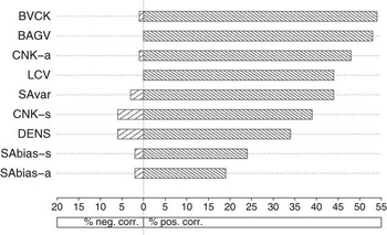
The best average testing results were achieved using the estimates BVCK, BAGV, CNK-a, LCV and SAvar in the decreasing order with respect to the percent of the significant positive correlations. The estimate SAbias-a achieved the worst average results. The comparison of the results, averaged across all regression models, is for all reliability estimates displayed in Figure 2.
Ranking of reliability estimates by the average percent of significant positive correlations with the prediction error (average percent of significant negative correlations is also displayed)

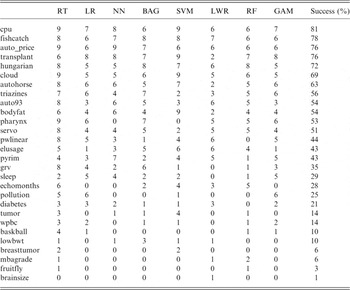
The results indicate that the estimates BVCK, SAbias, CNK, BAGV and LCV have a good potential for estimation of the prediction reliability. However, the results also showed that these estimates performed differently with different regression models and in different domains. This can be seen from Table 1, which shows a contingency of successful reliability estimates (i.e. estimates that significantly positively correlated to the prediction error) among testing domains and regression models (testing domains and model abbreviations are further described in Section 4). The dependence of the reliability estimates on the particular models and domains motivated us to explore approaches to automatic selection of the best-performing reliability estimate for a given domain and regression model. These are discussed in Sections 5 and 6.
The numbers of reliability estimates (out of nine) that were successful (achieved significant positive correlation to the prediction error) in different domains and using different regression models

RT = Regression trees; LR = Linear regression; NN = Neural networks; BAG = Bagging; SVM = Support vector machines; LWR = Locally weighted regression; RF = Random forests; GAM = Generalized additive model.
The rows are sorted in decreasing order of values in column Success that present a percentage of the successful estimates, averaged across all regression models. The ordering therefore ranks the domains by their difficulty of the reliability estimation task with the nine estimates at hand.
4 Experimental environment
We tested and compared the performance of nine individual estimates, presented in previous section (SAvar, SAbias-s, SAbias-a, BAGV, LCV, DENS, CNK-s, CNK-a and BVCK) to the performance of the two proposed approaches, presented in Sections 5 (internal cross-validation) and 6 (meta-learning). For each given domain and model, the most appropriate reliability estimate was first selected. Afterwards, the testing was performed using the leave-one-out cross-validation procedure. For each learning example that was left out in the current iteration, the prediction and all the tested reliability estimates were computed. Having completed all iterations, the leave-one-out errors and reliability estimates were therefore computed for all available examples. The performance of the reliability estimates was measured by computing the Pearson correlation coefficient between the reliability estimate and the prediction error. The significance of the correlation coefficient was afterwards statistically evaluated using t-test.
The testing was performed using eight regression models, implemented in statistical package R (R Development Core Team, 2006). In the following, we provide a brief description of some key properties of used models.
Regression trees (RT): Trees (Breiman et al., Reference Breiman, Friedman, Olshen and Stone1984) with the mean squared error used as the splitting criterion; the values in leaves represent the average label of corresponding training examples;
Linear regression (LR): Linear regression with no explicit parameters;
Neural networks (NN): Three-layered perceptron (Rumelhart et al., Reference Rumelhart, Hinton and Williams1986) with five hidden neurons, tanh activation function, the backpropagation learning algorithm using adaptive gradient descent;
Bagging (BAG): Bagging (Breiman, Reference Breiman1996) with 50 regression trees;
Support vector machines (SVM): The version of regression SVM (Vapnik, Reference Vapnik1995; Smola & Schölkopf, Reference Smola and Schölkopf1998), implemented in the LIBSVM library (Christiannini & Shawe-Taylor, Reference Christiannini and Shawe-Taylor2000; Chang & Lin, Reference Chang and Lin2001); When we used the third-degree RBF kernel, the precision parameter was ε = 0.1;
Locally weighted regression (LWR): Local regression with Gaussian kernel for weighting examples according to their distance;
Random forests (RF): Random forests (Breiman, Reference Breiman2001) with 100 trees;
Generalized additive model (GAM): Linear model (Hastie & Tibshirani, Reference Hastie and Tibshirani1990; Wood, Reference Wood2006) with no special parameters.
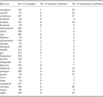
For testing we used 28 standard benchmark data sets, well known across the whole machine learning community. Each data set is a regression problem. The application domains vary from medical, ecological and technical to mathematical and physical domains. Most of the data sets are available from UCI Machine Learning Repository (Asuncion & Newman, Reference Asuncion and Newman2007) and from StatLib DataSets Archive (Department of Statistics at Carnegie Mellon University, 2005). All data sets are available from authors upon request. A brief description of data sets is given in Table 2.
Basic characteristics of testing data sets

5 Internal cross-validation
We adapted the basic cross-validation approach (Schaffer, Reference Schaffer1993) to select the most appropriate reliability estimate instead of the most appropriate learning algorithm. The proposed approach is described in the following.
5.1 Definitions
The internal cross-validation approach divides the learning examples to n equally sized subsets, as in the standard cross-validation approach. Each subset (selection set) is used for performance evaluation (correlation to the prediction error) of all testing reliability estimates. Based on acquired n correlation coefficients for each reliability estimate (one acquired between the estimate and the prediction error on each of the n subsets), the final (most appropriate) reliability estimate is selected as the one with the highest average correlation. This estimate is then used to estimate the reliability of all testing examples in that particular model and domain. The pseudocode of the procedure is shown in Figure 3.
The pseudocode for the internal cross-validation testing

5.2 Empirical evaluation
The testing was performed by correlating the reliability estimate, chosen by internal cross-validation procedure, with the prediction error of examples. The reliability estimate and the prediction errors were computed using the leave-one-out cross-validation procedure, that is, for each learning example that was left out in the current iteration. Having completed all iterations, the leave-one-out errors and reliability estimates were, therefore, computed for all available examples. The performance of the reliability estimates was measured by computing the Pearson correlation coefficient between the reliability estimate and the prediction error. The significance of the correlation coefficient was afterwards statistically evaluated using t-test for correlation coefficients with significance level α ⩽ 0.05.
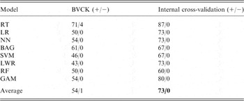
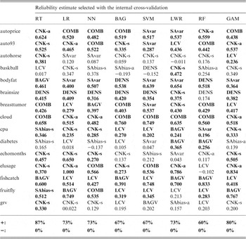
The summarized testing results are shown in Table 3 and the detailed results in Table 8 in the Appendix. Due to the extensive time complexity of nested cross-validation and the computation of all reliability estimates, it was not timely feasible to evaluate this approach on all available testing domains. The approach was, therefore, tested on the subset, consisting of 15 domains (brainsize, diabetes, elusage, sleep, pollution, mbagrade, pyrim, tumor, auto93, baskball, cloud, grv, fishcatch, autoprice, servo). To achieve representative results, these domains were approximately uniformly sampled from the ordering in Table 1 to include the domains with higher as well as with lower coverage by the reliability estimates.
The performance comparison of the most successful individual estimate BVCK and the estimate, selected with the internal cross-validation

RT = Regression trees; LR = Linear regression; NN = Neural networks; BAG = Bagging; SVM = Support vector machines; LWR = Locally weighted regression; RF = Random forests; GAM = Generalized additive model.
The table shows the percentage of experiments exhibiting significant positive/negative correlations between the reliability estimates and the prediction error.
The results show that the automatic selection of reliability estimates using the internal cross-validation achieved better performance than any of the individual testing estimates. We can see that on average, with the internal cross-validation the 73% of estimates significantly positively correlated with the prediction error, while 0% of estimates significantly negatively correlated with the prediction error. With the aim to compare this approach to another, possibly less time-demanding, we also propose a meta-learning approach, presented in the next section.
6 Meta-learning in domain/model problem space
To develop an approach for automatic prediction of the most appropriate reliability estimate, we also adapted the basic meta-learning approach (Aha, Reference Aha1992; Gama & Brazdil, Reference Gama and Brazdil1995). The proposed approach, which performs the estimate selection on the given domain and on the model basis, is defined and empirically evaluated in the following.
6.1 Definitions
Within our meta-learning approach we propose a meta-classifier, which is intended to predict the optimal reliability estimate for a given problem domain/regression model pair. The reliability estimates therefore represent class values to be predicted, the learning set consists of optimal selections for known domain/model pairs, and the attributes describe the domain/model characteristics that are related to a particular example.
Within this meta-learning task, a challenge arises on how to define the suitable meta-attributes. Since this task differs from meta-selecting the predictive model, we cannot rely on the fact that the same meta-attributes would be suitable for our task, as well. In addition, since the reliability estimates are model-independent, we cannot use attributes that extract specific model features, but can focus only on more general model description (i.e. performance of the model on particular domain). With this objective, we defined and proposed the following seven attributes for this meta-learning task:
• Regression model (discrete nominal attribute), used on a problem domain (in the following referred to as model);
• Number of learning examples in a given domain (no.examples);
• Number of attributes in a given domain (no.attr);
• Relative mean squared error, achieved by the given regression model on a domain using the tenfold cross-validation (cv.rmse);
• Average density of the problem space, estimated by Parzen windows and sampled in points, given by learning examples (avg.dens);
• Average distance to the five nearest neighbors, averaged across all learning examples (avg.DA);
• Average difference between the prediction for a given example and the predictions for the five nearest neighbors, averaged across all learning examples (avg.DK).
We can see that the attributes model, cv.rmse and avg.DK describe the regression model used, while the others provide a description of the data.
To each meta-learning example we assigned a class value, representing a reliability estimate that achieved maximum positive correlation with the prediction error (irrespective of whether the correlation was statistically significant or not) for a given regression model. The correlation coefficients between estimate values and prediction errors were computed using a leave-one-out scenario on each particular data set. The possible class values therefore were: SAvar, SAbias-s, SAbias-a, CNK-s, CNK-a, LCV, BAGV, DENS and BVCK.
6.2 Empirical evaluation
Since we experimented with 28 domains and 8 regression models, we, therefore, formed the meta-learning set consisting of 28 × 8 = 224 learning examples. To assure the unbiasedness of the testing procedure, in every experiment we removed the example from the meta-learning set that represented that domain/model combination, for which we were meta-predicting the optimal reliability estimate.
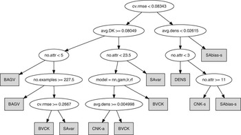
Meta-classifier. Using the above set of the meta-learning examples, we constructed a decision tree meta-classifier for prediction of the most appropriate reliability estimate. We decided to use the decision tree as the meta-model due to its interpretability, which helps us understand the decision on when the use of each estimate is more appropriate. An example of such decision tree (constructed on all 224 meta-learning examples, without removing any) is shown in Figure 4 (the tree was pruned using the 1-SE rule and the cost-complexity pruning algorithm (Breiman et al., Reference Breiman, Friedman, Olshen and Stone1984; Torgo, Reference Torgo2003)).
Meta-decision tree for prediction of the most appropriate reliability estimate

Although knowing that the performance of reliability estimates varies with different regression models, the results are rather interesting. We can see that the decision tree in Figure 4 shows that the most important attribute (more important than regression model), which constitutes the root node of the tree, is the RMSE, achieved by the given regression model on a domain using the tenfold cross-validation (cv.rmse). The tree shows that the estimates BAGV, BVCK, SAvar and CNK-a better perform with more accurate regression models, while the estimates DENS, CNK-s and SAbias-s better perform with less accurate regression models.
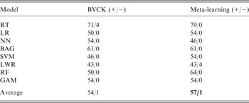
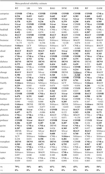
The testing results of the automatic selection of the best performing estimate using the meta-learning approach are shown in Table 4. The detailed results are shown in Table 7 in the Appendix. From comparison with the most successful (the largest number of significant positive correlations with the prediction error) individual reliability estimate BVCK we can see, that we achieved better average results using the meta-learning approach. However, compared to the results of the internal cross-validation approach (Table 3) we can see that the latter approach outperforms the meta-learning approach. Nevertheless, being less time-demanding and achieving better results than the most successful individual estimate BVCK, the proposed meta-learning approach shows the potential for predicting the domain/model-based optimal reliability estimate.
Performance comparison of the most successful individual estimate BVCK and the meta-predicted optimal estimate

RT = Regression trees; LR = Linear regression; NN = Neural networks; BAG = Bagging; SVM = Support vector machines; LWR = Locally weighted regression; RF = Random forests; GAM = Generalized additive model.
The table shows the percentage of experiments exhibiting significant positive/negative correlations between the reliability estimates and the prediction error.
Note that the present meta-learning approach requires further study (see Section 8). Besides evaluating stability and properties of the current meta-model, performance of other classifiers shall also be tested and evaluated. The current meta-learning problem shall also be optimized in terms of proposing/selecting more appropriate meta-attributes, using larger set of meta-examples and selecting the most appropriate set of target classes (i.e. set of reliability estimates).
7 Application on a real domain
The proposed methodology for automatic selection of the most appropriate estimate was preliminarily tested in a real domain. The data consisted of 1035 breast cancer patients, who had surgical treatment for cancer between 1983 and 1987 in the Clinical Center in Ljubljana, Slovenia. The patients were described using standard prognostic factors for breast cancer recurrence. The goal of the research was to predict the time of possible cancer recurrence after the surgical treatment. The analysis showed that this is a difficult prediction problem, because the possibility for recurrence is continuously present for almost 20 years after the treatment. Furthermore, the data present a mixture of two prediction problems, which additionally hinders the learning performance: (i) yes/no classification problem, whether the illness will recur at all, and (ii) the regression problem for the prediction of the recurrence time. In our study, the bare recurrence predictions were therefore complemented with our reliability estimates, helping the doctors with the additional validation of the predictions’ accuracies.
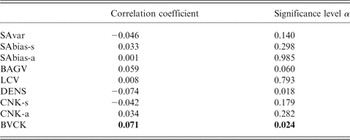
After the performance comparison of various regression models, the locally weighted regression was chosen for the use with this prediction problem, due to its low RMSE. For test examples, all nine available reliability estimates were computed, achieving the correlation to the prediction error as shown in Table 5. The statistical evaluation of the correlation coefficients revealed that only the estimate BVCK significantly positively correlates to the prediction error. This indicates that the oncological problem is a difficult domain for estimation of prediction reliability, in terms of domain ordering as shown in Table 1.
The correlation coefficients and their significance levels between the reliability estimates and the prediction error on the oncological application domain

On this particular problem, we tested both of our proposed methods for automatic selection of the most appropriate reliability estimate. Both, the internal cross-validation approach, as well as the meta-learning approach, selected the BVCK as the most appropriate estimate, which also turned out to be the optimal estimate for this problem, according to the results in Table 5. This result, therefore, shows the potential of the proposed methodology in practice.
8 Discussion
The testing of the individual reliability estimates, developed in our previous work, exhibited different potentials for the usage of different estimates with particular regression models. In addition, the results also showed that the success of the chosen reliability estimate may also be domain-dependent.
To deal with this problem, in the paper we proposed and tested two novel approaches for automatic selection of the most appropriate estimate for a given domain and regression model: the internal cross-validation approach and the meta-learning approach. With both approaches, the selection of estimates was performed from the set of nine estimates, based on various approaches, that is sensitivity analysis, variance of bagged models, local cross-validation, density-based estimation and local error estimation.
We implemented the internal cross-validation approach, which selects the most appropriate reliability estimate based on a subset of available examples. For the purpose of testing, we performed the partitioning as in standard cross validation, thus nesting the inner leave-one-out procedure (for computation of reliability estimates and the prediction error) in an outer tenfold cross-validation loop.
Next, we showed how reliability estimate selection can be turned into a meta-learning task by proposing meta-attributes and defining other meta-space parameters. By building a meta-decision tree classifier, we used it to predict a most appropriate reliability estimate for various domain and model combinations.
We compared the performance of both procedures for automatic selection of estimate, as well as to the performance of each individual estimate. The empirical results of both approaches showed the advantage of dynamically selected reliability estimate for a given domain/model pair, when compared to individual reliability estimates in terms of higher positive correlation to the prediction error. The best results were achieved using the internal cross-validation procedure. With this approach, the selected reliability estimates significantly positively correlated with the prediction error in 73% of domains and significantly negatively correlated with the prediction error in none.
Figure 5 displays a performance comparison of individual estimates and both approaches for the most appropriate estimate selection. The graphs show the percentage of experiments with the significant positive correlations (desired result) and the percentage of experiments with the significant negative correlation (undesired). We can see that internal cross-validation performed better than any of the other estimates in seven out of eight regression models. Meta-learning approach has empirically proven to perform good as well, since its performance was in top half of the ranking with all used regression models. The achieved results indicate that it is reasonable to approach the problem of automatic estimate selection using the proposed approaches.
Comparison (ranking) of meta-learning (META) and internal cross-validation (ICV) performance to the performance of individual reliability estimates. Graphs show the percent of experiments with the significant positive and negative correlations with the prediction error

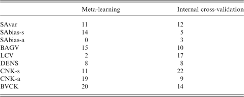
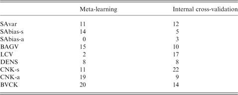
Comparison of both approaches. By analyzing how often was each of nine reliability estimates selected (in percent), as shown in Table 6, we can compare both of the proposed approaches. The comparison shows that the internal cross-validation approach most frequently selected such estimates that also perform well in specific domains (this can be seen by comparing Table 8 to detailed performance results of individual estimates, which cannot be presented here due to their extent—approximately 10 pages. The results are available from the authors on request). In contrast, the meta-learning approach most frequently selected the estimates that generally perform well also as individual reliability estimates, that is BVCK, BAGV and CNK-a.
The percent of each automatically selected reliability estimates using the meta-learning and internal cross-validation approach
We explain this phenomenon based on the main characteristics of both the approaches, as follows:
1. The proposed meta-learning approach is based on modeling of the dependence between the domain/model properties and the reliability estimate. By using the available meta-attributes, the meta-classifier’s predictive power is, therefore, limited by their descriptiveness of the particular domain and model. In contrast to this, the internal cross-validation operates directly with the available data and tests the candidate estimates on the subset of examples. If we assume that learning and test examples originate from the same distribution, it is likely that the estimate that correlates best with the prediction error on a subset of examples will also correlate well on the rest of the examples. This therefore enables the internal cross-validation approach to select estimates that are more tailored to the domain itself.
2. The purpose of the meta-learning approach is to induce a generalized rule for selection of the most appropriate estimate. This fact implies that, for preserving the generality of the rule (avoiding overfitting), the predicted estimates would most often be the ones that also perform well on average.
Time complexity of both approaches. The experiments showed that the internal cross-validation approach turned out to be more demanding than the meta-learning approach. Since reliability estimates are independent of a particular regression model, we discuss the time complexity of both approaches in terms of the number of regression models they require to be constructed.
The design of the internal cross-validation approach shows that nine reliability estimates have to be computed in the two nested loops (10 times leave-one-out procedure), out of which the most demanding estimate BAGV requires constructing 50 regression models for each example. Considering other reliability estimates (SAvar and SAbias require ten models, LCV five and CNK one), this therefore means that for testing domain with 100 examples, at least 6600 models would need to be constructed.
We can discuss the complexity of the meta-learning approach from the following two perspectives: the complexity of generating the meta-learning set (which depends on the proposed meta-attributes) and the complexity of modeling and predicting the final estimate. The former requires computing six meta-attributes, which include computing distances, local models and prediction errors. Among these attributes, the computation of the RMSE is the most time-consuming (tenfold cross-validation requires constructing ten models). Not considering computing distances and auxiliary costs, this means that for computation of the meta-learning set of size 100, we would require construction of 1000 models. In contrast, the other complexity perspective of the meta-learning approach (generating the final model and predicting the most appropriate estimate) requires inducing of only one model.
The case of our study shows that the greater time complexity of the internal cross-validation approach clearly pays off with its better performance.
Further work. The achieved results in the field of estimating reliability for individual predictions offer the challenges for further work, which includes:
• A good correlation of signed reliability estimates (SAbias-s and CNK-s) with the signed prediction error implies the potential for the usage of reliability estimates for the correction of regression predictions. We shall, therefore, explore whether these two reliability estimates can be utilized to reduce the error of regression predictions.
• Different performances of reliability estimates in different testing domains (see Table 1) indicate that the potential for estimation of prediction reliability is in some domains more feasible than in the others. The domain characteristics, which lead to a good performance of reliability estimates, shall be analyzed in more detail.
• The meta-learning approach shall be further analyzed by employing other predictive models, proposing new attributes and evaluating their quality.
• The preliminary experiments with meta-learning have shown that the selection of a regression model with low RMSE and the selection of a model on which reliability estimates will perform well, is a trade-off criteria. This phenomenon shall be analyzed in further theoretical and empirical work.
Appendix A: Detailed results
Automatically selected reliability estimates using the meta-predictor and their correlation coefficients with the prediction error

RT = Regression trees; LR = Linear regression; NN = Neural networks; BAG = Bagging; SVM = Support vector machines; LWR = Locally weighted regression; RF = Random forests; GAM = Generalized additive model.
Statistically significant values (α ⩽ 0.05) are denoted with boldface. Significant negative values (undesired negative correlations) are additionally underlined.
Automatically selected reliability estimates using internal cross-validation and their correlation coefficients with the prediction error

RT = Regression trees; LR = Linear regression; NN = Neural networks; BAG = Bagging; SVM = Support vector machines; LWR = Locally weighted regression; RF = Random forests; GAM = Generalized additive model.
Statistically significant values (α ⩽ 0.05) are denoted with the boldface. There were no significant negative values (undesired negative correlations).