





1. Introduction
The response of wall-bounded flows to prescribed spatio-temporal wall modulation provides a canonical setting for isolating how boundary forcing alters near-wall structure, instability growth and the route to turbulence. A natural reference state is the zero-pressure-gradient (ZPG) flat-plate boundary layer, whose transition routes have been studied extensively. In low-disturbance environments, instability develops through the exponential amplification of Tollmien–Schlichting (TS) waves, followed by secondary instability, vortex breakdown and turbulent-spot formation (Schubauer & Skramstad Reference Schubauer and Skramstad1947; Schlichting et al. Reference Schlichting, Gersten and Krause2000; Saric et al. Reference Saric, Reed and White2003). Under stronger environmental disturbances, transition may proceed through bypass routes involving the amplification of streaks, shear-layer instabilities and rapid breakdown (Kendall Reference Kendall1985; Reshotko Reference Reshotko2001; Matsubara & Alfredsson Reference Matsubara and Alfredsson2001; Fransson et al. Reference Fransson, Brandt, Talamelli and Cossu2005a ). As both pathways are receptive to surface non-uniformity and imposed forcing, prescribed wall geometry and motion provide controlled means of modifying the transition onset, location and mechanism.
Static sinusoidal wall geometry has been studied for decades as a generator of separation, secondary instability and modified turbulence production, where periodic crests and troughs redistribute momentum, impose alternating pressure gradients and may generate separated shear layers that modify instability growth and turbulence production (Lin et al. Reference Lin, Walsh, Watson and Balasubramanian1983; Abrams & Hanratty Reference Abrams and Hanratty1985; Hudson et al. Reference Hudson, Dykhno and Hanratty1996; De Angelis et al. Reference De Angelis, Lombardi and Banerjee1997; Günther & Rudolf Von Rohr Reference Günther and Rudolf Von Rohr2003; Kruse et al. Reference Kruse, Kuhn, von and von Rohr2006; Hamed et al. 2015, 2016; Yang et al. Reference Yang, Sadique, Mittal and Meneveau2016; Martins Segunda et al. Reference Martins Segunda, Ormiston and Tachie2018). Stability analyses have shown that corrugation-induced base-flow distortion can destabilise TS-like modes and introduce centrifugal, three-dimensional (3D) and transient-growth mechanisms (Floryan Reference Floryan1997; Cabal et al. Reference Cabal, Szumbarski and Floryan2002; Floryan Reference Floryan2005; Asai & Floryan Reference Asai and Floryan2006; Floryan Reference Floryan2002, Reference Floryan2007; Szumbarski & Floryan Reference Szumbarski and Floryan2006; Mohammadi et al. Reference Mohammadi, Moradi and Floryan2015). Thus, even without temporal motion, periodic wall geometry can reorganise the mean flow and its instability spectrum.
Travelling-wave walls add a second mechanism through the propagation speed of the imposed surface pattern. Linear analyses have shown that wall vibrations can strongly amplify disturbances when their wavelength and frequency approach those of neutral TS waves, while detuning produces weaker or transient responses (Floryan et al. Reference Floryan, Szumbarski and Wu2002; Floryan & Zandi Reference Floryan and Zandi2019). Related studies have identified wavenumber lock-in, parametric resonance and interactions between multiple imposed patterns (Hossain et al. Reference Hossain, Floryan and Floryan2012; Floryan & Floryan Reference Floryan and Floryan2015; Floryan & Inasawa Reference Floryan and Inasawa2021; Hossain & Floryan Reference Hossain and Floryan2022).
For a travelling wave with frequency
 $f$
, wavelength
 $\lambda$
and phase speed
 $c=f\lambda$
, the phase-speed ratio
 $\textit{St}_w=c/U_\infty =f\lambda /U_\infty$
, where
 $U_{\infty}$
is the freestream velocity, can be written in a Strouhal-like form and compares the propagation speed of the boundary pattern with the free-stream velocity. The present standing-wave wall instead has a spatially stationary pattern, and its forcing is characterised by the convection-based Strouhal number
 $\textit{St}=f_w\lambda /U_{c,m}=f_w/f_{\textit{conv}}$
, which compares the wall-oscillation frequency with the convection frequency of the coherent structures. The wall deflection may be represented as
 $\eta (x,t)=a\sin (2\pi x/\lambda )\cos (2\pi f_wt)$
, which oscillates in time about a fixed streamwise-periodic shape and therefore has zero net streamwise phase propagation. Shen et al. (Reference Shen, Zhang, Yue and Triantafyllou2003) considered a streamwise-travelling wall-normal deformation in fully turbulent flow at
 $\textit{Re}_\lambda \approx 10\,170$
, where
 $\textit{Re}_\lambda$
is the Reynolds number based on the wall wavelength. In contrast, the present study examines how a spatially stationary, time-periodic wall-normal deformation affects laminar-to-turbulent transition.
A combined experimental and numerical approach is adopted because the two methods provide complementary capabilities for the present problem. The experiments establish the physical realisability and repeatability of the standing-wave wall forcing under controlled low-disturbance conditions and provide validation data for the evolving transitional boundary layer. The direct numerical simulation (DNS), in turn, provides phase-resolved access to coherent structures and the instability dynamics over a broader range of forcing frequencies than is experimentally practical. The approaches are also complementary in parameter space: low-frequency forcing is experimentally favourable because the long oscillation periods would require prohibitively long DNS integration times for converged statistics, whereas higher-frequency forcing is more efficiently explored numerically due to the demanding temporal-resolution requirements of phase-locked experiments.
Using this combined framework, we investigate boundary-layer development over a surface undergoing sinusoidal standing-wave oscillations. Our goal is to uncover the physical mechanisms by which standing-wave wall forcing modifies boundary-layer growth, transition location and the organisation of coherent motions. By systematically varying the wall-oscillation frequency across 18 cases, we isolate its role in advancing or delaying transition and show that the non-monotonic response results from reinforcing and suppressing phase relations between the wall motion and convecting shear-layer structures. The study therefore identifies a transition regime controlled not only by wall waviness but also by the synchronisation between the imposed forcing and the intrinsic boundary-layer dynamics.
The remainder of the paper is organised as follows. Section 2 describes the custom-designed wind-tunnel facility and the DNSs. Section 3 presents the principal observations and analysis, with emphasis on synchronisation effects, transition modulation and the evolution of coherent structures. Section 4 discusses the broader implications of the results, and § 5 summarises the main findings and outlines directions for future work.
(
 $a$
) Basic schematic of the customised wind tunnel illustrating reference dimensions, (
 $b$
) Measured actuated surface at four instants used in the phase-locked PIV: envelopes and negligible amplitudes.

Figure 1. Long description
Panel A: A diagram of a customized wind tunnel setup. The setup includes four adjustable DC fans with honeycomb-shaped flow straighteners, an elliptical contraction, and a high-speed 80 W laser. The wind tunnel has a length of approximately 1.3 meters and a width and height of approximately 0.305 meters. A standing wavy wall with a wavelength of 100 mm and amplitude of 5 mm is actuated at frequencies of 0.5, 1, 2, and 4 Hz. The mechanical system includes high-speed 4 MP CMOS cameras and synchronized DC motors connected to central shafts. Panel B: A graph showing the measured actuated surface at four instants used in phase-locked particle image velocimetry (PIV). The graph plots the wall displacement (y_w) against the non-dimensionalized x-axis (x/λ) and shows the envelopes and negligible amplitudes of the wavy wall at different phases.
2. Experimental and numerical set-ups
The experiments and DNSs were designed to mirror one another as closely as possible in geometry and forcing conditions, enabling direct cross-validation while exploiting the complementary strengths of each approach.
2.1. Laboratory experiments
Laboratory experiments were conducted in a specially designed, open-circuit, pressure-type wind tunnel equipped with an adjustable standing-wave wall. The test section has a cross-section of 308 mm
 $\times$
308 mm and a length of 1.3 m. Upwind of the test section, a larger chamber with four identical DC fans, power-supply controlled, provides the flow. The chamber transitions into an elliptical contraction with a 4 : 1 area ratio, followed by a double-layer flow straightener, a 200-mm-long smooth inlet, an 800-mm-long flexible wall with eight sinusoidal standing waves, and a 305 mm downstream smooth section. To ensure high-flow uniformity, the flow-conditioning section includes honeycomb grids with a cell size of 3.2 mm, which effectively suppress non-uniformities and residual swirl. Although the tunnel design differs from traditional suction-type facilities, it provides fully controlled inflow conditions with uniform mean velocity and negligible free-stream turbulence. Repeatability and inflow stability were checked by measuring incoming flow fields and turbulence levels before each run and over time; the mean drifts were negligible.
In the scenario with flat wall, the flow exhibited a canonical Blasius boundary-layer profile with free-stream turbulence intensity below 0.1 %, as verified by particle image velocimetry (PIV). For the corresponding smooth flat-plate boundary layer, the Reynolds number based on the displacement thickness,
 $\textit{Re}_{\delta ^\ast }$
, reaches approximately 524 at the downstream end of the measurement domain, which is close to the classical critical value
 $\textit{Re}_{\delta ^\ast ,\textit{crit}} \approx 520$
associated with the onset of TS instability in low-disturbance ZPG flows. This indicates that, in the absence of wall waviness and temporal forcing, the baseline boundary layer remains nominally subcritical over most of the test section; the observed transition is therefore attributed to the imposed wall geometry and its controlled standing-wave modulation.
A customised mechanical actuation system integrated into the bottom wall of the wind tunnel generates standing waves with adjustable frequency. The oscillatory wall consists of a 3.2 mm thick impermeable polyvinyl chloride foam sheet supported by sixteen ribs spaced 50 mm apart. The flexible wall forms eight standing waves, each with a wavelength of
 $\lambda = 100$
mm and amplitude
 $a = 5$
mm. The foam is fixed at the wave nodes by rigid supports to ensure repeatable boundary conditions and smooth curvature during operation. Each rib is driven by an individual cam mounted on a common camshaft, which is mechanically phased such that adjacent ribs oscillate with a
 $180^{\circ }$
phase difference, thereby producing the desired standing-wave pattern. The camshaft is powered by a stepper motor, allowing for precise control of rotational speed and, consequently, the wall-oscillation frequency. The system can accommodate either a static flat wall or an actuated wavy wall. A general schematic of the facility is shown in figure 1(a), where the origin of the streamwise coordinate,
 $x = 0$
, is defined at the leading edge of the actuated surface, and the vertical coordinate,
 $y = 0$
, is defined at the mean wall position at the start of the wavy section.
The standing-wave wall motion introduces a spatio-temporal forcing through a prescribed wall displacement of the form
 $y_w(x,\varphi )=a\cos (2\pi x/\lambda +\pi /2 )\sin (\varphi )$
, where
 $\varphi =2\pi (1/4+f_w t)$
. The developing boundary layers were characterised using PIV at wall frequencies
 $f_w=0$
,
 $1/2$
, 1, 2 and 4 Hz at the same
 $\textit{Re}_a = U_{\infty }a/\nu \approx 390$
(or bulk
 $\textit{Re}_H = U_{\infty } H / \nu = 2.4 \times 10^{4}$
), where
 $U_{\infty }$
denotes the free-stream velocity at the beginning of the standing waves,
 $\nu$
is the kinematic viscosity of air and
 $H$
the test-section height. To accurately capture and monitor the wall motion, the experiments included tracking the wall by imaging the deforming surface at a sampling frequency of 240 Hz for the
 $f_w=1/2$
and 1 Hz cases, and at 480 Hz for the
 $f_w=2$
and 4 Hz scenarios (see figure 1
b).
The PIV measurements were conducted in two modes: time resolved and phase locked. Time-resolved measurements were performed at a sampling rate of 200 Hz over a field of view
 $x/\lambda \in [6,7]$
and
 $y/a\in [-1,10]$
, yielding 3600 velocity fields. Phase-locked measurements were acquired using two partially overlapping fields of view spanning
 $x/\lambda \in [5, 7.5]$
and
 $y/a \in [-1, 10]$
. For each frequency case, a total of 8400 velocity fields were collected, with 2100 fields acquired at each of the four phases
 $(\varphi /\pi = 0, 1/2, 1, 3/2)$
. For the static wavy-wall case, 2400 velocity fields were obtained. The PIV measurements employed single- and dual-camera configurations using 4 MP Phantom M340 CMOS sensors with a resolution of 2560
 $\times$
1600 pixels. Flow seeding was achieved using nebulisers (Philips InnoSpire Essence) generating approximately
 $1\,{\unicode[Arial]{x03BC}}$
m particles. Illumination was provided by a 50 mJ diode-pumped 527 nm Nd:YLF laser for time-resolved measurements and a 250 mJ double-pulsed 532 nm Nd:YAG laser for phase-locked measurements, producing a laser sheet of approximately 1 mm thickness. These configurations yielded spatial resolutions of
 $\Delta x=320$
and 780
 ${\unicode[Arial]{x03BC}}$
m (with 50 % overlap) for time-resolved and phase-locked measurements, respectively. More than 95 % of velocity vectors were validated across all datasets, and phase triggering was confirmed to be stable within each oscillation cycle. To present the PIV parameters in non-dimensional form, the Kolmogorov length and time scales,
 $\eta$
and
 $\tau _\eta$
, were estimated from the energy dissipation rate following Tanaka & Eaton (Reference Tanaka and Eaton2007) and Gomes-Fernandes et al. (Reference Gomes-Fernandes, Ganapathisubramani and Vassilicos2012). The resulting dimensional and non-dimensional PIV parameters are summarised in table 1.
Particle image velocimetry measurement and DNS sampling parameters used for comparison. DNS fields were interpolated onto a uniform Cartesian grid.

Table 1. Long description
The table compares particle image velocimetry (PIV) and direct numerical simulation (DNS) sampling parameters. It has three columns labeled PIV, Kolmogorov-scaled, and DNS, and four rows labeled Grid spacing, Sampling interval, Sampling duration, and Field of view. Row 1: Grid spacing, 320 micrometers; 0.8 times Delta x times eta less than or equal to 1.4; (Delta x, Delta y) equals (333, 366) micrometers. Row 2: Sampling interval, 5 milliseconds; 0.4 times Delta t times eta less than or equal to 0.8; 1.66 milliseconds. Row 3: Sampling duration, 18 seconds; 1500 times T times eta less than or equal to 3400; 1 second times 350 z-planes. Row 4: Field of view, 100 times 55 square millimeters; 238 times Lx times eta less than or equal to 454; 800 times 55 square millimeters.
2.2. Numerical simulations
Direct numerical simulations were performed using NekRS (Fischer et al. Reference Fischer2022) which is a GPU-accelerated version of Nek5000, a NEAMS open-source computational fluid dynamics solver. The NekRS solver is based on the spectral element method, which combines rapid convergence and tensor-product efficiency with the geometric flexibility of the finite element method for solution of the incompressible Navier–Stokes equations. It is especially suited to the simulation of transitional and turbulent flows in complex geometries. We used a dimensionless formulation of the incompressible governing equations
 \begin{equation} \frac {\partial \boldsymbol{u}}{\partial t} + \boldsymbol{u} \boldsymbol{\cdot }\boldsymbol{\nabla }\boldsymbol{u} = -\boldsymbol{\nabla }\!p + \frac {1}{\textit{Re} _a} \boldsymbol{\nabla} ^2\boldsymbol{u} \quad \text{and} \quad \boldsymbol{\nabla }\boldsymbol{\cdot }\boldsymbol{u} = 0, \end{equation}
where
 $\boldsymbol{u}$
and
 $p$
are the velocity and pressure field. These equations are cast into their weak form and spatially discretised using Nth-order Lagrange interpolants on Gauss–Lobatto–Legendre (GLL) points for both velocity and pressure fields. Time integration is performed using NekRS’s second-order semi-implicit splitting scheme. A constant non-dimensional time step corresponding to a maximum Courant–Friedrichs–Lewy number of 0.5 was chosen to ensure numerical stability and adequate temporal resolution of the smallest scales. At each step, the velocity–pressure coupling is enforced through a preconditioned conjugate gradient solver for the pressure Poisson equation, with a relative residual tolerance of
 $10^{-6}$
.
At the inlet, a spatially varying inhomogeneous Dirichlet velocity boundary condition is prescribed. To represent the experimental inflow downstream of the honeycomb flow straighteners, the mean streamwise velocity is constructed from a laminar boundary-layer profile modulated by a localised hexagonal-cell pattern. The baseline vertical variation is given by a fitted Blasius-type profile, while within each honeycomb cell the streamwise velocity is adjusted using a two-dimensional (2D) Gaussian modulation. The hexagonal pattern is generated by tiling the inlet plane with regular hexagonal cells of side length
 $s$
, giving a streamwise-periodic unit cell of width
 $\sqrt {3}\,s$
and height
 $3s$
. For each inlet point, the local in-plane coordinates are reduced modulo these periodic lengths, and the distance
 $r$
is defined as the minimum distance to the centres of the five surrounding hexagonal-cell cores in the unit-cell construction. The honeycomb modulation is then prescribed as
 $G(r)=\exp (-r^2/\sigma ^2 ),$
where
 $\sigma$
controls the width of the cell-core region and is taken proportional to the side length, here
 $\sigma = s/2$
. The streamwise velocity is finally written as the fitted boundary-layer profile multiplied by a weak honeycomb correction proportional to
 $G(r)-\overline {G}$
, where
 $\overline {G}$
is a constant chosen so that the modulation has zero mean over the repeating cell pattern. In the present set-up,
 $s=0.3666$
and
 $\sigma =0.1833$
in non-dimensional units. This synthetic honeycomb pattern is repeated periodically across the inlet plane to match the cross-sectional structure of the flow straightener. Low-amplitude perturbations are superimposed on the transverse velocity components to represent residual disturbances introduced by the inflow hardware. These perturbations generate a three-component (3C) turbulence intensity of approximately
 $0.5\,\%$
at the inlet, consistent with a low-disturbance laboratory inflow. All production simulations use this honeycomb-modulated inflow with weak fluctuations. At the outlet, pressure is stabilised using the method of Dong et al. (Reference Dong, Karniadakis and Chryssostomidis2014). The flat surfaces at the top and bottom are treated as no-slip static walls corresponding to homogeneous Dirichlet velocity boundary conditions. The sinusoidal walls undergo the prescribed standing-wave motion, with zero velocity in the streamwise and spanwise directions and a vertical velocity determined by the imposed oscillation. In contrast to the experiments, which can capture a large number of snapshots for statistical averaging, the simulations would require significantly longer runtimes to achieve similar temporal statistics. To compensate, periodic boundary conditions are applied in the spanwise direction, enabling efficient spanwise averaging.
A conforming hexahedral mesh of
 $210\times 50\times 50$
spectral elements spans the streamwise, spanwise and vertical directions, respectively. The vertical element sizes are distributed according to GLL spacing to provide finer resolution near the wall and accurately capture boundary-layer structures. With a seventh-order polynomial representation within each element, the discretisation yields a total of 268.8 million grid points. For comparison with the planar PIV measurements, the DNS solution was interpolated from the spectral element GLL mesh onto a uniform Cartesian grid during post-processing. Due to the periodic spanwise boundary conditions, each stored DNS snapshot provides 350 statistically equivalent spanwise planes. Consequently, a physical sampling duration of 1 s corresponds to an effective planar sampling duration of approximately 350 s when compared with single-plane PIV measurements. Simulations were carried out on leadership-class GPU systems at the Argonne Leadership Computing Facility and the Oak Ridge Leadership Computing Facility, using a fixed decomposition of 96 MPI ranks, with one rank assigned per GPU tile/GCD. To reduce the influence of start-up transients, each case was initialised from a previously converged solution. The simulation was then advanced for approximately ten flow-through times to allow residual transients to leave the computational domain. After statistical stationarity was reached, flow statistics were accumulated over an additional twelve flow-through times.
The DNSs of developing boundary layers considered 16 scenarios with wall frequencies of
 $f_w=0$
, and 4–15 Hz in increments of 1 Hz, as well as 18, 21 and 24 Hz. Due to the large size of the data set, only the 0, 4, 6, 12, 18, 21 and 24 Hz cases were selected to store with full streamwise extent of
 $x/\lambda \in [0,8]$
. However, all cases were saved for a limited streamwise extent of
 $x/\lambda \in [6,7]$
, as every case except the 24 Hz case experienced transition before or within this region. All of the stored data were 2D-two-component (2C) data and saved with sampling frequency of 600 Hz with a number of snapshots between 1600 and 3600. The experiments and simulations overlapped at scenarios with
 $f_w=0$
(static wavy wall) and 4 Hz to test and validate the approaches. To calculate phase-averaged statistics, triple decomposition was used to decompose the signal into mean, periodic and turbulent component. Starting from the Reynolds decomposition
 \begin{equation} u_i(\boldsymbol{x},t) = U_i(\boldsymbol{x}) + u_i'(\boldsymbol{x},t), \end{equation}
where
 $\boldsymbol{x}$
,
 $t$
,
 $u_i$
,
 $U_i$
and
 $u_i'$
denote the Eulerian coordinate, time, instantaneous velocity, time-averaged velocity and velocity fluctuations, respectively. The triple decomposition partitions the velocity fluctuation component
 $u_i'$
further into a deterministic periodic component and a stochastic turbulent component. Specifically,
 \begin{equation} {u_i}(\boldsymbol{x},t) = {U_i}(\boldsymbol{x}) + \tilde {u_i}(\boldsymbol{x},\varphi ) + {u_i''}(\boldsymbol{x},t), \end{equation}
 \begin{equation} \langle u_i\rangle =U_i+\tilde {u}(\boldsymbol{x},\varphi ), \end{equation}
where
 $\langle \boldsymbol{\cdot }\rangle$
is the phase-averaging operator,
 $\tilde {u_i}$
is the phase-locked, coherent response synchronised with the wall motion and
 $u_i''$
is the residual, uncorrelated turbulent fluctuation. For more details on triple decomposition, see Reynolds & Hussain (Reference Reynolds and Hussain1972). Figure 2 compares the phase-averaged statistics between the experimental and simulation cases, showing very good agreement. The normalised 2D cross-correlation was computed to quantify the similarity between the experimental and simulated contours shown in figures 2(g) and 2(h), yielding a coefficient of approximately 0.8, which supports the validity of the simulation results.
Comparison between experiments and numerical simulations for the scenario under standing waves at
 $f=4$
Hz at
 $\varphi =\pi /2\,(a{-}d)$
and
 $\varphi =\pi \,(e{-}h)$
with (
 $a,e$
) streamwise velocity,
 $\langle u\rangle /U_{\infty }$
, and (
 $b,f$
) vertical velocity,
 $\langle v\rangle /U_{\infty }$
, (
 $c,g$
) phase-averaged turbulence intensity,
 $\sqrt {\langle {u''}^2\rangle }/U_{\infty }$
, and (
 $d,h$
) phase-averaged kinematic shear stress
 $- \langle {u''v''}\rangle /U_{\infty }^2$
. Black curves indicate profiles at intervals of
 $\Delta x/\lambda =1/4$
.

3. Results
The response of the boundary layer to the dynamic wavy wall is first organised in terms of the non-dimensional parameters that describe the coupling between wall forcing and coherent-structure convection. The wall motion imposes both a fixed spatial scale,
 $\lambda$
, and a forcing frequency,
 $f_w$
, so the relevant time-scale comparison is between the wall-oscillation period and the time required for coherent structures to convect over one wavelength. We therefore first estimate the convective velocity and define the reduced frequency,
 $\textit{St}$
, in § 3.1. Using
 $\textit{St}$
as the organising parameter, we then examine the time- and phase-averaged statistics in § 3.2, boundary-layer characteristics in § 3.3, phase interaction between wall motion and coherent-structure convection in § 3.5, spectral features in § 3.6 and secondary effects in § 3.7.
3.1. Convection-velocity estimation
Because the standing-wave wall imposes both a fixed spatial wavelength,
 $\lambda$
, and a temporal frequency,
 $f_w$
, the flow response can be organised by comparing the wall-oscillation period with the time required for coherent structures to convect over one wavelength. We therefore use the reduced frequency
 \begin{equation} \textit{St}=\frac {f_w\lambda }{U_{c,m}} =\frac {f_w}{f_{\text{ conv}}} =\frac {\lambda }{\lambda _w}, \end{equation}
where
 $f_{\text{ conv}}=U_{c,m}/\lambda$
and
 $\lambda _w=U_{c,m}/f_w$
is the distance travelled by a coherent structure during one wall-oscillation period. Near-integer values,
 $\textit{St}\approx n$
, correspond to recurrence at approximately the same wall phase, whereas near-half-integer values,
 $\textit{St}\approx n+1/2$
, produce an approximately
 $\pi$
-shifted phase. As shown below, the near-integer and near-half-integer cases are associated with suppressing and reinforcing interactions, respectively.
The mean convection velocity
 $U_{c,m}$
was estimated by following the method of Dennis & Nickels (Reference Dennis and Nickels2008) as the structure of experimental and simulation data is planar 2D-2C data. Other estimation methods that require spanwise gradient (del Álamo & Jiménez Reference del Álamo and Jiménez2009) or 3D-3C (Lozano-Durán & Jiménez Reference Lozano-Durán and Jiménez2014) data were not able to be applied here. The method of Dennis & Nickels (Reference Dennis and Nickels2008) was adapted to address the strong periodicity in the Reynolds-decomposed fluctuation component, which arises from the periodic wall modulation
 \begin{equation} R_{u''u''} (\Delta x,y,\Delta t) = \frac {\overline {u''(x,y,t)u''(x+\Delta x,y,t+\Delta t)}}{u''_{\textit{rms}}(y)u''_{\textit{rms}}(y)}. \end{equation}
The convection velocity at each vertical height,
 $U_{\text{ conv}}(y)$
, was obtained from the slope of the dominant peak ridge in the space–time correlation map defined in (3.2). This procedure was applied to the triple-decomposed fluctuation,
 $u_i''$
, rather than to the Reynolds fluctuation, because the latter retains a strong phase-locked component associated with the wall motion. At higher forcing frequencies, this periodic contribution produces multiple correlation ridges and obscures the convective ridge associated with the turbulent structures. Using
 $u_i''$
removes the deterministic wall-locked component and yields a more robust estimate of structure convection across the transitional region.
For cases with full streamwise data over
 $x/\lambda \in [0,8]$
, the domain was divided into windows of length
 $\lambda$
with 50 % overlap, and (3.2) was applied within each window, as shown in figure 3. The local boundary-layer thickness,
 $\delta _{95}$
, was obtained from the streamwise-averaged mean velocity profile over the same window. The convection-velocity profiles show spatial convergence by the downstream windows. For the
 $f_w=12$
and
 $21\,\mathrm{Hz}$
cases, fewer upstream profiles could be resolved because distinct correlation peaks were not always identifiable; however, the difference between the final two windows was negligible. The window
 $x/\lambda \in [6,7]$
was therefore used to compute
 $U_{c,m}$
because it satisfied this convergence criterion and provided the broadest data coverage across cases. As shown in figure 4, the resulting convection velocities remain close to the standard estimate for boundary-layer coherent structures,
 $U_c\approx 0.8U_\infty$
. Thus, the purpose of this analysis is not to establish a new convection-velocity scaling, but to provide a consistent case-by-case estimate of
 $U_{c,m}$
for calculating
 $\textit{St}$
. The mean convection velocity, obtained by averaging
 $U_{\text{ conv}}$
from the first near-wall point to
 $y=\delta _{95}$
, ranges between
 $0.79 \leqslant U_{c,m}/U_\infty \leqslant 0.85$
. For the 24 Hz case, where no distinct correlation peak could be identified,
 $U_{c,m}=0.8U_\infty$
was used to compute
 $\textit{St}$
.
Development of convection velocity in the streamwise direction. Here,
 $\delta _{95}$
was calculated with mean streamwise velocity profile averaged in each window.

Figure 3. Long description
Five line graphs depict the development of convection velocity in the streamwise direction under different conditions. Each graph represents a different wall modulation frequency (4 Hz, 6 Hz, 12 Hz, 18 Hz, and 21 Hz). The x-axis represents the normalized convection velocity (U_conv/U_infinity), and the y-axis represents the normalized wall-normal coordinate (y/delta_95). Each line within a graph corresponds to a different range of x/lambda values, as indicated by the legend. The colors of the lines vary to distinguish between different x/lambda ranges. The graphs show how the convection velocity changes with the wall-normal coordinate for each frequency and x/lambda range. The trends indicate the influence of wall modulation on the flow structure and transition to turbulence.
Convection velocity at
 $x/\lambda \in [6,7]$
. Here,
 $\delta _{95}$
was calculated with mean streamwise velocity profile averaged in the window.

Figure 4. Long description
A line graph with the horizontal axis labeled U conv over U infinity ranging from 0.6 to 1.0 and the vertical axis labeled y over delta 95 ranging from 0.2 to 1.0. The graph includes multiple lines representing different frequencies: 4 H z, 6 H z, 8 H z, 10 H z, 11 H z, 12 H z, 13 H z, 14 H z, 15 H z, 18 H z, and 21 H z. Each line shows a trend of how the normalized convection velocity changes with normalized height for the respective frequency. The lines generally show an upward trend, indicating an increase in normalized convection velocity with increasing normalized height.
It is important to note that the convective velocity within a turbulent boundary layer is not a singular, absolute metric; its calculated value inherently depends on the chosen method and spatial points or boundaries. Consequently, the values of
 $U_{c,m}$
and the resulting
 $\textit{St}$
may vary depending on one’s specific operational definition. Rather than presenting these as universally absolute values, the objective of this approach is to establish a mathematically rigorous and internally consistent framework for this specific study. By applying this systematic definition across all cases, we can robustly characterise the dynamic coupling between the wall oscillation and the overlying turbulent structures using
 $\textit{St}$
.
3.2. Time- and phase-averaged statistics
(
 $a$
) Time-averaged streamwise velocity, (
 $b$
) turbulence kinetic energy and (
 $c$
) kinematic shear stress, time-averaged quantities for several oscillation periods, over oscillating walls relative to the wall surface,
 $y_w$
, for wall frequencies
 $\textit{St}=0.41$
(experiments),
 $\textit{St}=0.62$
(earliest transition, simulations) and
 $\textit{St}=1.2$
(latest transition, simulations).

The time-averaged statistics for selected reduced frequencies,
 $\textit{St}=0.41$
, 0.62 and 1.2, at
 $x/\lambda \in [6, \ 7]$
are presented in figure 5, showing contours of the mean streamwise velocity, in-plane turbulent kinetic energy (TKE),
 $ (\overline {u'^2} + \overline {v'^2}) / 2U_\infty ^2$
and Reynolds shear stress,
 $- \overline {u'v'}/U_\infty ^2$
, where the over-bar is time-averaging operator. For the standing-wave cases, the mean velocity field expressed relative to the instantaneous wall position,
 $y-y_{w\textit{all}}$
, does not show the strong streamwise modulation typical of a canonical static wavy-wall boundary layer. Instead, the time-averaged streamwise velocity is comparatively uniform along
 $x$
for the frequencies shown. This behaviour differs from the static wavy-wall measurements of Hudson et al. (Reference Hudson, Dykhno and Hanratty1996), where the boundary-layer structure depends strongly on the phase along the wave. Thus, in a time-averaged sense, the mean boundary-layer structure is not simply locked to the local wall geometry. Nevertheless, changing
 $f_w$
produces systematic differences in boundary-layer thickness: the
 $\textit{St}=0.41$
and
 $\textit{St}=1.2$
cases are noticeably thinner than the
 $\textit{St}=0.62$
case. This thickness variation indicates distinct transitional pathways, implying that wall forcing does not simply superimpose periodic motion but alters the conditions for instability growth. The differences are not limited to boundary-layer thickness; as shown later, they coincide with changes in the coherence and spatial distribution of turbulence production, revealing a delicate interplay between wall-induced forcing, shear-layer roll-up, and transition onset.
Instantaneous snapshot of coherent vortical structures over the standing-wave wall at
 $f_w=6$
Hz, with
 $\lambda _2=-0.005$
iso-surface coloured by the local velocity magnitude. It illustrates the onset of turbulence and the downstream growth of vortical complexity, with initially organised wave-induced structures evolving into increasingly 3D coherent motions over successive wavelengths.

Figure 6. Long description
Panel: A visualization of coherent vortical structures over a standing-wave wall. The iso-surface is colored by the local velocity magnitude. The structures show the onset of turbulence and the downstream growth of vortical complexity, with initially organized wave-induced structures evolving into increasingly 3D coherent motions over successive wavelengths.
Experimental phase-averaged statistics at
 $\textit{St}=0.10$
.
 $(a,b)$
Streamwise velocity,
 $\langle u \rangle /U_\infty$
,
 $(c,d)$
phase-averaged turbulence intensity,
 $\sqrt {\langle {u''}^2 \rangle } /U_\infty$
, and
 $(e,f)$
kinematic shear stress,
 $-\langle u''v''\rangle /U_\infty ^2$
. The phase of figures on the left column
 $(a,c,e)$
is
 $\varphi =\pi /2$
and the phase of figures on the right column
 $(b,d,f)$
is
 $\varphi =\pi$
.

Figure 7. Long description
Panel A: A heat map showing streamwise velocity at phase 0. The x-axis is labeled x/λ and ranges from 5.25 to 7.25. The y-axis is labeled y/a and ranges from 0 to 8. The color scale ranges from 0 to 1, with blue indicating lower values and red indicating higher values. The velocity is higher near the top and lower near the bottom. Panel B: A heat map showing streamwise velocity at phase π. The axes and color scale are the same as in Panel A. The velocity distribution is similar but slightly different in pattern. Panel C: A heat map showing phase-averaged turbulence intensity at phase 0. The x-axis is labeled x/λ and ranges from 5.25 to 7.25. The y-axis is labeled y/a and ranges from 0 to 8. The color scale ranges from 0 to 0.20, with blue indicating lower values and red indicating higher values. The turbulence intensity is higher near the top and lower near the bottom. Panel D: A heat map showing phase-averaged turbulence intensity at phase π. The axes and color scale are the same as in Panel C. The turbulence intensity distribution is similar but slightly different in pattern. Panel E: A heat map showing kinematic shear stress at phase 0. The x-axis is labeled x/λ and ranges from 5.25 to 7.25. The y-axis is labeled y/a and ranges from 0 to 8. The color scale ranges from 0 to 8, with blue indicating lower values and red indicating higher values. The shear stress is higher near the top and lower near the bottom. Panel F: A heat map showing kinematic shear stress at phase π. The axes and color scale are the same as in Panel E. The shear stress distribution is similar but slightly different in pattern.
Figures 5(b) and 5(c) present the TKE and Reynolds shear-stress fields. The two lower-frequency cases (
 $\textit{St}=0.41$
and 0.62) exhibit intensified regions of TKE and shear stress, consistent with enhanced shear-layer activity. The DNS predicts a larger magnitude of Reynolds shear stress than the PIV in figure 5(c). Nevertheless, the dominant shear-stress structure appears at a similar
 $x/\lambda$
location and exhibits comparable inclination and spatial organisation in both datasets. These regions originate from the local flow separation over the wave crests, induced by the adverse pressure gradients inherent to the wall geometry, and mark the onset of rapid amplification of the dominant horseshoe-shaped vortices, as shown in figure 6. It illustrates iso-surfaces of
 $\lambda _2$
coloured by velocity magnitude where
 $\lambda _2$
is the second largest eigenvalue of
 $\mathcal{S}^2+ {\varOmega }^2$
, where
 $\mathcal{S}$
and
 ${\varOmega }$
denote the symmetric and antisymmetric parts of the velocity-gradient tensor (Jeong & Hussain Reference Jeong and Hussain1995). The associated growth of TKE and momentum exchange reflects a more efficient transfer of energy from the mean flow to the fluctuating field. This behaviour is consistent with observations from static wavy-wall flows (Hudson et al. Reference Hudson, Dykhno and Hanratty1996; De Angelis et al. Reference De Angelis, Lombardi and Banerjee1997; Kruse et al. Reference Kruse, Kuhn, von and von Rohr2006; Hamed et al. Reference Hamed, Kamdar, Castillo and Chamorro2015), where increased production near separation zones accelerates the development of turbulent boundary layers.
In contrast, the
 $\textit{St}=1.2$
case displays a broader distribution of TKE, while its Reynolds shear-stress field forms an alternating lobe pattern (last row of figure 5). The regions of strong shear stress are confined closer to the wall and exhibit a sharper negative peak, indicating enhanced damping of instability amplification. The more spatially uniform TKE field, together with this organised shear-stress pattern, suggests that turbulence at
 $\textit{St}=1.2$
is sustained primarily by local energy input from the oscillating boundary rather than by outer-layer shear-layer interactions. This behaviour differs fundamentally from the
 $\textit{St}=0.41$
and 0.62 cases, where turbulence intensification arises from the growth and breakdown of coherent vortical structures convected along the wavy surface.
To isolate phase-specific features of the wall motion, figure 7 illustrates phase-locked fields for
 $x/\lambda \in [5,\ 7.5]$
at the phases of maximum and minimum wall displacement for
 $\textit{St}=0.10$
. Shown are the phase-averaged mean velocity, streamwise turbulence intensity and Reynolds shear stress. At this comparatively low frequency, the flow organises into a separation-driven shear layer akin to that over a directly measured static wavy-wall case (not shown for the brevity) and Hudson et al. (Reference Hudson, Dykhno and Hanratty1996) which had same roughness to wavelength ratio. In figure 7(a), no closed reverse-flow region is observed in the phase-averaged streamwise velocity field, unlike what is typically expected for a static wavy wall with comparable
 $a/\lambda$
. This difference reflects the unsteady nature of the standing-wave forcing: shear-layer structures generated near the crest do not remain fixed over the downslope region, but are convected downstream as the wall shape evolves. At maximum wall displacement, figures 7(c) and 7(e) show a pronounced crest-originating shear layer that persists for nearly one wavelength, accompanied by elevated turbulence intensity and Reynolds shear stress. This shear-layer development is consistent with prior observations over static wavy walls of comparable
 $2a/\lambda$
(Hudson et al. Reference Hudson, Dykhno and Hanratty1996).
At the vanishing wall amplitude phase, separation is absent. However, the previously formed shear layer, and the associated regions of high TKE and Reynolds shear stress, do not vanish; rather, figure 7
 $b$
shows that it deforms, adopting a more uniform thickness in the streamwise direction. Consistently, figures 7(d) and 7( f) reveal that the peaks of turbulence intensity and Reynolds shear stress are displaced downstream relative to their locations at maximum amplitude. This phase-to-phase evolution indicates that the dominant coherent structure does not break down immediately but retains its identity as it convects and reshapes downstream, providing a mechanistic link between crest-triggered separation and subsequent amplification during the oscillation cycle.
(
 $a$
) Normalised boundary-layer thickness,
 $\delta _{95}/a$
, at node locations
 $x/\lambda =6$
and 7 as a function of reduced frequency,
 $\textit{St}$
. Horizontal grid lines mark the mean value for the Blasius solution and static sinusoidal wall within that region. (
 $b$
) Mean streamwise velocity contour,
 $U/U_\infty$
, within
 $x/\lambda \in [6,\ 7]$
for maximum and minimum
 $\delta _{95}/a$
cases.

Figures 5 and 7 reveal that wall-oscillation frequency modulates boundary-layer transition through several interacting mechanisms. Increasing the oscillation frequency injects additional energy from the moving boundary, yet this input remains largely confined to the near-wall region where viscous effects dominate. Higher
 $\textit{St}$
alters the effective pressure-gradient landscape experienced by the convecting flow, reshaping the balance between favourable and adverse segments across each wave. Most importantly, the imposed wall motion can either amplify or attenuate the convection of dominant coherent structures depending on their phase relationship with the oscillation. When forcing and convection are synchronised, constructive interaction strengthens shear-layer roll-up and promotes earlier transition; when out of phase, destructive interference suppresses amplification and delays it. These coupling effects form the physical basis for the frequency-dependent modulation examined in the following section.
3.3. Boundary-layer characteristics
To evaluate the impact of wall oscillations on boundary-layer development, and to connect these effects with the previously discussed shear-layer formation and convection mechanisms, we focus on the representative region
 $x/\lambda \in [6,7]$
, where transition consistently occurs across all cases.
Figure 8(a) shows the normalised boundary-layer thickness,
 $\delta _{95}/a$
, as a function of wall-oscillation frequency
 $\textit{St}$
. Here
 $\delta _{95}$
, the vertical location where the time-averaged mean velocity reaches 95 % of the free-stream value, is used as a consistent measure of boundary-layer thickness among all configurations. The results demonstrate that standing-wave forcing can either thin or thicken the boundary layer depending on
 $\textit{St}$
. In certain regimes,
 $\delta _{95}$
drops below the classical Blasius prediction for a flat plate, whereas in others it increases markedly, even surpassing the static wavy-wall reference. This variation spans more than a factor of two, highlighting the high sensitivity of boundary-layer growth to oscillation frequency. Distinct minima in
 $\delta _{95}$
appear at
 $\textit{St}=1.2$
and
 $2.5$
, while maxima occur around
 $\textit{St}\approx 0.62$
and
 $1.8$
. These alternating bands of enhanced and suppressed growth are clearly visible in figure 8(b) (specifically at
 $\textit{St}=0.62$
and
 $1.2$
). Between these frequencies,
 $\delta _{95}$
exhibits an almost linear variation with
 $\textit{St}$
, suggesting a quasi-periodic modulation of the mean boundary-layer thickness with the wall-forcing cycle.
Boundary-layer thickness development:
 $(a)$
development of the normalised boundary-layer thickness,
 $\delta _{95}/a$
, across the full streamwise domain compared against the Blasius solution; and
 $(b)$
focused downstream development of the normalised boundary-layer thickness deviation,
 $(\delta _{95}-\delta _{\textit{Blasius}})/a$
, isolating a targeted subset of reduced frequencies that exhibit boundary-layer suppression. Shaded regions denote areas of localised boundary-layer suppression relative to the Blasius profile.

Figure 9 presents the streamwise evolution of the normalised boundary-layer thickness,
 $(\delta _{95}-\delta _{\textit{Blasius}})/a$
, for several wall-oscillation frequencies. Comparison with the Blasius flat-plate reference reveals distinct growth patterns across frequencies. At
 $\textit{St}=1.2$
and 1.8, the boundary layer follows a Blasius-like evolution up to
 $x/\lambda \approx 6.2$
and
 $4.8$
, respectively, before diverging as transition occurs. These cases illustrate that oscillatory forcing can modulate the rate of boundary-layer development and postpone the onset of turbulence. Such behaviour cannot be attributed solely to the unsteady pressure gradients induced by the wall motion; it reflects instead the combined effect of wall forcing and large-scale shear-layer dynamics. The dependence of
 $\delta _{95}/a$
on
 $\textit{St}$
further reveals a frequency-selective response, suggesting that the transition is governed by the phase synchronisation between the imposed wall motion and the convective transport of dominant coherent structures.
Iso-surfaces of coherent motions (
 $\lambda _2$
= -0.005) over standing waves at various wall frequencies,
 $f_w$
. Blue-dashed enclosures show the maximum turbulence transition delay crisis at reduced frequencies
 $\textit{St}=1.2$
and 2.5.

Figure 10. Long description
Panel A: A series of visualizations showing iso-surfaces of coherent motions over standing waves at different wall frequencies. The frequencies range from 0 to 10 Hz, with corresponding Strouhal numbers (St) indicated. Panel B: Another series of visualizations showing iso-surfaces of coherent motions over standing waves at different wall frequencies. The frequencies range from 11 to 24 Hz, with corresponding Strouhal numbers (St) indicated. Blue-dashed enclosures highlight the maximum turbulence transition delay crisis at specific reduced frequencies and Strouhal numbers.
3.4. Transition to turbulence
Figure 10 illustrates iso-surfaces of
 $\lambda _2$
and reveal how the transition location and structure of coherent vortices vary with wall-oscillation frequency. As
 $\textit{St}$
increases, the emergence and convection of vortical structures shift downstream, highlighting the frequency-dependent modulation of transition. Supplementary Movies 1–3 are available at https://doi.org/10.1017/jfm.2026.12137 provide the corresponding time-resolved dynamics for the static wall and for the oscillating cases at
 $\textit{St}=0.62$
and 1.2, capturing the formation, deformation and downstream propagation of the dominant coherent motions. The earlier transitions occur at
 $\textit{St}\in [0.41,\ 0.62]$
and [1.5, 1.8], whereas delayed transitions appear at
 $\textit{St}=1.2$
and 2.5, revealing alternating regimes of constructive and destructive coupling between the imposed wall motion and the convective dynamics of the flow.


A central feature of the flow response is the relationship between the reduced frequency,
 $\textit{St}$
, and the transition location,
 $x_{\text{ tr}}$
, shown in figure 11. The transition point is quantitatively defined using an intermittency criterion described in Appendix A. The dependence of
 $x_{\text{ tr}}/\lambda$
on
 $\textit{St}$
exhibits a quasi-periodic pattern across the investigated range of
 $f_w$
cases, alternating between early and delayed transition as the phase relation between wall forcing and convective motion shifts. This trend is represented as the sum of a monotonic baseline and an oscillatory departure
 \begin{equation} \frac {x_{\text{ tr}}}{\lambda } \approx c_0 + c_1 \textit{St} + c_2 \cos \left (\frac {2\pi }{T} \textit{St} + \phi \right )\!, \end{equation}
where
 $c_0+c_1\textit{St}$
describes the baseline downstream shift of transition with increasing
 $\textit{St}$
, while the cosine term captures the alternating advance and delay associated with constructive and destructive phase coupling. The parameters were obtained in two steps. First, a linear fit was used to estimate and remove the monotonic baseline, where this baseline can be interpreted as decreasing effective slope or pressure-gradient effects as wall-forcing frequency increases (which will be discussed again in § 3.7). A nonlinear least-squares fit was then applied to the detrended residuals to determine the oscillatory component, giving
 $c_1\approx 2.3$
,
 $c_2\approx 1.4$
,
 $T\approx 1.3$
and
 $\phi \approx 0.32\pi$
. It is worth pointing out that
 $\textit{St}$
is dependent on the
 $U_{c,m}$
estimation; thus, the fitted period value is sensitive to the convection-velocity definition discussed in connection with (3.2) and shown in figure 4. Indeed, the fitted
 $T\approx 1.3$
for
 $U_{c,m}/U_\infty \approx 0.8$
maps to a free-stream normalised period
 $T_\infty =(U_{c,m}/U_\infty )T\approx 1.0$
, consistent with the possibility that the coherent structures convect increasingly close to
 $U_\infty$
as they develop and move away from the near-wall region downstream. This fit of (3.3), indicated by the solid black line in figure 11, is used only as a compact empirical description of the observed trend, not as a predictive law.
This captures the alternating constructive and destructive coupling between the wall oscillation and the convection of coherent structures. The fit is not intended as a predictive law, but as a concise empirical representation of the observed phase-locked response. For
 $\textit{St} \approx 0.62$
, transition occurs early near
 $x_{\text{ tr}}/\lambda \approx 2$
, whereas increasing
 $\textit{St}$
toward
 $1.2$
results in a pronounced delay, with
 $x_{\text{ tr}}/\lambda$
reaching 6–7. Beyond this range, the trend reverses, dropping to 4–5 near
 $\textit{St} \approx 1.7$
before rising again to approximately 7.5 at
 $\textit{St} \approx 2.2$
. This oscillatory dependence reflects the alternating synchronisation states between the imposed wall motion and the convective transport of coherent structures: constructive alignment near
 $\textit{St} \approx 0.62$
and
 $1.7$
accelerates transition, while destructive dephasing near
 $\textit{St} \approx 1.2$
and
 $2.2$
suppresses instability growth. At higher forcing frequencies (
 $\textit{St}\gtrsim 1.2$
), the transition location shifts downstream but remains phase locked to the same pattern, highlighting the persistence of frequency–flow coupling across the examined range.
The results indicate that resonance between the wall oscillation and the convection of coherent structures governs the modulation of boundary-layer transition. When the forcing and convective time scales align (
 $\textit{St}\approx$
0.62 and 1.7), phase lock-in enhances the amplification of shear-layer instabilities and accelerates the breakdown process. At
 $\textit{St}\approx 1.2$
, however, the phase relationship becomes destructive, weakening the coupling between wall forcing and coherent-structure convection, which suppresses boundary-layer growth and delays transition. While the present analysis isolates the influence of oscillation frequency, the amplitude of wall motion is also expected to affect the strength of coupling and the spatial extent of lock-in, a topic to be explored in future work.
3.5. Phase interaction between wall oscillation and convection of coherent structures
 $(a)$
Time series of streamwise (solid) and vertical (dashed) velocity fluctuations, and kinematic shear stress, at
 $(x/\lambda ,\ y/a)=(2,\ 2.5)$
(location marked by
 $\times$
in
 $(b)$
).
 $(b)$
Representative
 $\lambda _2$
snapshots showing instantaneous velocity fields for
 $\textit{St}=0.62$
(
 $f_w=6$
Hz).

Figure 12. Long description
Panel A: Two line graphs show time series of streamwise (solid line) and vertical (dashed line) velocity fluctuations, and kinematic shear stress. The x-axis represents normalized time (t/T) ranging from 0 to 3, and the y-axis represents normalized velocity fluctuations and shear stress. The graphs display periodic fluctuations over time. Panel B: Eight snapshots of instantaneous velocity fields are shown, each corresponding to a specific normalized time point (t1/T to t8/T). The x-axis represents normalized distance (x/λ) ranging from 0 to 3, and the y-axis represents normalized height (y/a) ranging from 0 to 4. Each snapshot shows the distribution of velocity fields with marked points and arrows indicating specific features.
 $(a)$
Time series of streamwise (solid) and vertical (dashed) velocity fluctuations, and kinematic shear stress, at
 $(x/\lambda ,\,y/a)=(7,\,2.5)$
(location marked by
 $\times$
in
 $(b)$
).
 $(b)$
Representative
 $\lambda _2$
snapshots showing instantaneous velocity fields for
 $\textit{St}=1.2$
(
 $f_w=12$
Hz).

Close inspection of the
 $\lambda _2$
fields and representative streamwise and vertical velocity fluctuations,
 $u'$
and
 $v'$
, provides insight into how the phase relationship between wall oscillation and the convection of dominant coherent structures governs boundary-layer transition. Two characteristic cases are examined:
 $\textit{St} = 0.62$
and
 $\textit{St} = 1.2$
, corresponding to the early and delayed-transition scenarios shown in figures 12 and 13, respectively.
At
 $\textit{St} = 0.62$
, the convective velocity of the coherent structures nearly matches the phase velocity,
 $f_w\lambda$
, of the wall oscillation, establishing phase synchronisation between the forcing and convective time scales, as illustrated in figure 12(b). Lock-in initiates when shear-layer instability emerges on the adverse-pressure-gradient (APG) side of the first wavy element (arrow at
 $t=t_1$
). Because the convective time over one wavelength is then comparable to the forcing period, the structures reappear over successive APG regions at nearly the same phase of the wall motion. This phase recurrence maintains coherence across wavelengths and promotes cumulative amplification of the shear layer. Although passage through favourable-pressure-gradient (FPG) regions locally weakens the growth, it does not eliminate the phase organisation established over the APG portions of the wall. The resulting resonance-like reinforcement accelerates the transition and produces a thicker boundary layer, as reflected in the increase in
 $\delta _{95}/a$
, along with enhanced turbulence production over a substantial wall-normal extent. This interpretation is consistent with the elevated TKE and Reynolds shear-stress peaks shown in figures 5(b) and 5(c).
At higher forcing frequencies, the shortened oscillation period reduces the effective pressure gradient and limits the interaction between the oscillating wall and the APG regions, thereby suppressing large-scale shear-layer instability and producing a distinct transition pathway. A representative case,
 $\textit{St} = 1.2$
, is shown in figure 13. The
 $\lambda _2$
field reveals elongated, streak-like near-wall structures generated by the rapid wall motion, a characteristic feature observed in all cases with
 $\textit{St} \ge 1.2$
. Intermittent packets of small-scale coherent structures are also evident (figure 13
 $b$
), which undergo localised breakdown and gradually trigger transition. However, the ratio of convective to forcing time scales primarily determines the onset, the phase interactions remain relevant even in high-frequency regime as evidenced by the earlier transition onset for the
 $\textit{St}=1.8$
case compared with the
 $\textit{St}=1.2$
case.
For
 $\textit{St}\approx 1.2$
and 2.2, the forcing and convection cycles are out of phase, leading to destructive interference between wall-induced oscillations and shear-layer instability. As a result, coherent structures are alternately displaced between the APG and FPG zones, where their growth is inhibited during FPG passages. The net effect is a suppression of cumulative amplification, yielding a more persistent laminar or weakly transitional boundary layer that extends farther downstream when compared with the synchronised
 $\textit{St}$
cases.
Time series of
 $-\lambda _2/|\lambda _2|_{max}$
at selected flow cases and downstream locations at a fixed height of
 $y/a=3$
:
 $\textit{St}=0.62$
,
 $x/\lambda =2$
and
 $(b)$
 $\textit{St}=1.2$
 $x/\lambda =6.5$
.

Spectra of
 $\lambda _2$
at a fixed height of
 $y/a=3$
for selected wall-frequency scenarios:
 $(a)\,\textit{St}=0.62$
and
 $(b)\,\textit{St}=1.2$
. Black, red, green and blue colours denote
 $(a)\, x/\lambda =1$
, 1.5, 2, 2.5 and
 $(b)\, x/\lambda =5.5$
, 6, 6.5 and 7.

3.6. Spectral features
Spectral analysis of the
 $\lambda _2$
signal at
 $y/a=3$
provides quantitative insight into the periodic evolution of coherent structures. The
 $\lambda _2$
field directly reflects vortex organisation, though care must be taken in interpreting the
 $\textit{St}=1.2$
case, where elevated
 $\lambda _2$
values not associated with convecting structures are also present (figure 13). Representative time series of
 $\lambda _2$
are shown in figure 14. For
 $\textit{St}=0.62$
(figure 14
 $a$
), the signal exhibits strong periodicity at the wall-forcing period
 $T_w$
, consistent with the cyclic convection of coherent structures seen in figure 12. Secondary modulations occur within each cycle, marking the onset of structural breakdown; this pattern persists throughout the record. In contrast, the
 $\textit{St}=1.2$
case (figure 14
 $b$
) lacks persistent periodicity, showing instead intermittent, sharp peaks corresponding to sporadic vortex packets, in agreement with figure 13.
The corresponding frequency spectra (figure 15) further highlight these contrasting regimes. At
 $\textit{St}=0.62$
, a pronounced spectral peak appears at
 $f/f_w=1$
, with secondary harmonics present, indicating strong synchronisation between the wall oscillation and the convective dynamics of coherent structures. By contrast, at
 $\textit{St}=1.2$
(figure 15
 $b$
), the spectrum is broadband and lacks a dominant peak at
 $f/f_w=1$
, confirming the loss of phase synchronisation and the prevalence of intermittent, non-periodic activity characteristic of the dephased regime.
Further insight is gained by examining how spectral energy evolves downstream. At
 $\textit{St} = 0.62$
, the amplitude of the dominant spectral peak increases progressively with streamwise distance up to the transition point (
 $x_{\text{ tr}}/\lambda = 2.2$
), indicating the gradual amplification of coherent structures as they convect downstream. This behaviour arises from the near match between the convective velocity and wall-wave speed, which maintains phase lock-in and allows structures initiated in the APG regions to amplify cumulatively until breakdown. In contrast, at
 $\textit{St} = 1.2$
, no distinct peaks are present at
 $f/f_w$
or its harmonics across the streamwise domain. Instead, the spectral energy exhibits an abrupt broadband rise between
 $x/\lambda = 5.5$
and 6, marking a rapid onset of turbulence, in contrast to the gradual amplification observed at
 $\textit{St}=0.62$
.
3.7. Secondary effects
Beyond phase interaction, boundary-layer development as
 $\textit{St}$
varies is also influenced by the pressure-gradient environment experienced by the convecting structures. For lower forcing frequencies, such as
 $\textit{St}=0.41$
–0.62, coherent packets seeded at the APG crests grow into an outer shear layer and feed turbulence production over a substantial vertical extent, consistent with the high TKE and Reynolds shear-stress peaks in figures 5(b) and 5(c). At higher forcing frequencies, such as
 $\textit{St}=1.2$
, the direct viscous response remains confined closer to the wall: the Reynolds shear stress forms alternating near-wall lobes, and the TKE field becomes more spatially uniform rather than organised around discrete packet roll-up. This indicates that, at high
 $\textit{St}$
, turbulence is maintained primarily through local energy input from the oscillating wall with limited coupling to the outer shear layer, whereas at lower
 $\textit{St}$
it is driven by packet amplification and roll-up that extend farther into the boundary layer.
Increasing wall-oscillation frequency shortens the forcing time scale and effectively weakens the pressure gradients perceived by the flow. As a result, the mean streamwise velocity profile progressively approaches that of a canonical flat-plate boundary layer (figure 16
 $a$
). In contrast, at lower
 $\textit{St}$
the flow more strongly follows the wall waviness, producing an internal boundary layer whose modulation extends well into the outer region (figure 16
 $b$
). Thus, although the directly forced viscous region becomes thinner as
 $\textit{St}$
increases, the weakened outer-shear-layer amplification dominates, shifting transition downstream.
Mean streamwise velocity profiles at
 $x/\lambda =6.5$
for selected wall-oscillation frequencies.
 $(a)$
Profiles plotted as a function of
 $y/a$
.
 $(b)$
Same data with logarithmic vertical scale to emphasise near-wall variation.

Figure 16. Long description
Panel A: A line graph shows mean streamwise velocity profiles as a function of y/a. The x-axis represents U/U∞, and the y-axis represents y/a. The graph includes multiple data series for different Strouhal numbers (St) and a reference line labeled Blasius. Panel B: Another line graph presents the same data with a logarithmic vertical scale to emphasize near-wall variation. The x-axis represents U/U∞, and the y-axis represents U/U∞ on a logarithmic scale. Different symbols represent various Strouhal numbers.
Although all cases ultimately transition to turbulence by the downstream end (figure 10), which was discussed in § 3.4, the boundary layers evolve through markedly different developmental paths. First-order estimates of characteristic parameters help quantify this modulation. In particular, the friction velocity
 $u_\ast$
, aerodynamic roughness length
 $z_0$
, and displacement height
 $d_0$
capture the effect of wall forcing on near-wall momentum transfer, especially under vertical wall motion. These quantities are linked to the approximated logarithmic law of the wall
 \begin{equation} \frac {U}{u_\ast } = \frac {1}{\kappa } \ln \left (\frac {y - d_0}{z_0}\right )\!, \end{equation}
where
 $\kappa \approx 0.41$
is the von Kármán constant. The friction velocity is estimated from the normalised Reynolds shear stress,
 $\overline {u'v'}/u_\ast ^2$
, while
 $d_0$
and
 $z_0$
are obtained from semi-logarithmic fits to the mean velocity profiles.
Table 2 summarises the resulting parameters for three representative conditions: early transition (
 $\textit{St} = 0.62$
), maximum transition delay (
 $\textit{St} = 1.2$
) and the Blasius reference case. The wall shear stress
 $\tau _w$
and
 $u_\ast = (\tau _w/\rho )^{1/2}$
increase in the synchronised regime (
 $\textit{St} = 0.62$
), consistent with intensified momentum transfer and enhanced turbulent production. The delayed-transition case (
 $\textit{St} = 1.2$
) exhibits lower
 $u_\ast$
and reduced displacement height, reflecting weaker wall–flow coupling and a more stable boundary-layer configuration.
Estimated boundary-layer parameters at
 $x/\lambda \approx 7.5$
-8 for two standing-wave cases with distinct reduced frequencies
 $\textit{St}$
. The Blasius flat-plate case is included for reference.

Table 2. Long description
The table presents boundary-layer parameters for three conditions: Blasius, St = 0.62, and St = 1.2. It has four rows and five columns. The columns are labeled Parameter, Blasius, St = 0.62, and St = 1.2. The rows are labeled with different parameters: δ95 [mm], u* [m s⁻¹], d0/a, and z0/a. The values in the table are as follows: Row 1: δ95 [mm], Blasius 2.9, St = 0.62 5.6, St = 1.2 3.2. Row 2: u* [m s⁻¹], Blasius 0.041, St = 0.62 0.076, St = 1.2 0.067. Row 3: d0/a, Blasius 0, St = 0.62 0.20, St = 1.2 0. Row 4: z0/a, Blasius —, St = 0.62 0.016, St = 1.2 0.015.
These quantities, together with the streamwise evolution shown in figure 9, show the contrasting effects of wall forcing on boundary-layer development. For
 $\textit{St} = 0.62$
, the boundary-layer thickness is approximately 70 % greater than that for
 $\textit{St} = 1.2$
. The synchronised case (
 $\textit{St} = 0.62$
) also exhibits higher
 $u_\ast$
and a non-zero displacement height
 $d_0$
, consistent with intensified vertical momentum exchange and a raised effective roughness origin produced by the wall’s vertical motion. The presence of
 $d_0\gt 0$
indicates a measurable aerodynamic blockage effect arising from oscillatory forcing, signalling an active, turbulence-generating regime. In contrast, the dephased case (
 $\textit{St} = 1.2$
) displays reduced
 $\delta _{95}$
and
 $u_\ast$
, with negligible displacement height, suggesting that the imposed oscillations at this frequency impart minimal blockage and insufficient energy input to sustain a fully developed turbulent state. The correspondingly lower
 $z_0$
and weaker shear are consistent with a delayed transition and suppressed turbulent activity in this regime.
4. Discussion
The laminar–turbulent transition over oscillating wavy walls emerges from the subtle interplay between phase synchronisation, and pressure-gradient modulation. Rather than a single trigger, transition is governed primarily by the coordinated action of phase matching between wall forcing and coherent-structure convection, represented by the reduced frequency
 $\textit{St}$
, and the alternating adverse and FPGs imposed by the wall geometry. Constructive interaction between phase alignment and the pressure-gradient sequence promotes transition, while destructive interference suppresses it. As
 $\textit{St}$
approaches regions (
 $\textit{St}\approx 0.62, 1.7$
), the wall-oscillation period becomes commensurate with the convective time scale of dominant structures, resulting in phase synchronisation or lock-in. In this regime, structures repeatedly interact with the APG crests in phase, reinforcing shear-layer roll-up and enhancing energy transfer into the boundary layer. By contrast, when
 $\textit{St}$
is near 1.2 and 2.2, the wall motion and structure convection are dephased; the APG exposure weakens, the amplification loop collapses, and the transition is delayed. The resulting oscillatory variation of
 $x_{\text{ tr}}/\lambda$
with
 $\textit{St}$
reflects alternating constructive and destructive synchronisation bands.
Thus, transition modulation is attributed primarily to phase coupling between wall motion, pressure-gradient forcing and coherent-structure convection.
The transition pathways are organised primarily by
 $\textit{St}$
. In lock-in conditions, wall-induced oscillations remain phase aligned with the convecting structures over successive APG regions, thereby intensifying Reynolds shear and kinetic energy production. In dephased conditions, the near-wall response is out of sync with the convecting structures, resulting in weaker coupling, reduced shear and a delayed transition. Increasing the oscillation frequency further shortens the effective exposure to APG segments, diminishing the net pressure gradient perceived by the flow and driving the mean profile toward a canonical flat-plate behaviour. These mechanisms collectively define a compact parametric picture in which
 $\textit{St}$
governs phase synchrony. The identification of these trends provides a mechanistic basis for phase-aware transition control: certain
 $\textit{St}$
bands favour coherent energy transfer and early transition, whereas others promote stability and laminar persistence. The observed macroscopic transition shifts are attributed to phase coupling between wall motion, pressure-gradient forcing and coherent-structure convection.
5. Conclusions
The combined experimental and numerical evidence leads to the central conclusion that transition over a standing-wave wall is governed not by the forcing frequency alone, but by its phase relation with coherent-structure convection, as captured by
 $\textit{St}=f_w\lambda /U_{\mathit{c,m}}$
. The wall therefore acts as a phase-selective modifier of instability growth, capable of either advancing or delaying transition at a fixed deformation amplitude.
Two complementary effects determine the transition location. Increasing
 $\textit{St}$
shortens the exposure to the wall-induced pressure-gradient sequence, weakens outer-shear-layer amplification, and shifts transition downstream on average. Superposed on this trend, near-half-integer
 $\textit{St}$
produces reinforcing interactions that advance transition, whereas near-integer
 $\textit{St}$
produces suppressing interactions that delay it. The monotonic baseline and oscillatory departures are therefore consequences of pressure-gradient attenuation and phase recurrence, respectively.
The distinct spectral and structural signatures further show that phase coupling changes the route to transition rather than merely shifting the location of an otherwise unchanged process. Reinforcing interactions promote organised, outer-layer-connected disturbance growth, whereas suppressing interactions confine activity closer to the wall and postpone shear-layer breakdown. Agreement between the experiments and DNSs indicates that this interpretation is not specific to either method. Its persistence at higher
 $\textit{Re}_a$
, with only a modest shift of the
 $\textit{St}$
bands, suggests that the mechanism is robust, although its precise thresholds retain some Reynolds-number dependence.
Because the wave amplitude was fixed and the Reynolds-number range was moderate, the empirical linear-plus-cosine relation should be viewed as an organising description of the investigated regime rather than a universal predictive law. Establishing such a law will require determining how
 $\textit{Re}_a$
,
 $a/\lambda$
and waveform affect the convection velocity, monotonic baseline and phase-band boundaries. Nevertheless, our results establish the practical hypothesis that transition can be controlled by tuning wall oscillations to the coherent-structure convection time scale rather than selecting them solely by forcing frequency or amplitude. Whether this phase-based strategy yields drag, noise, or other performance benefits remains to be tested in higher-Reynolds-number and application-specific flows.
Supplementary movies
Supplementary movies are available at https://doi.org/10.1017/jfm.2026.12137.
Funding
P.F. was supported by the U.S. Department of Energy, Office of Science, under contract DE-AC02-06CH11357. This research used resources of the Argonne Leadership Computing Facility, a U.S. Department of Energy (DOE) Office of Science user facility at Argonne National Laboratory and is based on research supported by the U.S. DOE Office of Science-Advanced Scientific Computing Research Program, under Contract No. DE-AC02-06CH11357. This research also used resources of the Oak Ridge Leadership Computing Facility at the Oak Ridge National Laboratory, which is supported by the Office of Science of the U.S. Department of Energy under Contract No. DE-AC05-00OR22725.
Declaration of interests
The authors report no conflict of interest.
Appendix A. On the laminar-to-turbulent transition
To characterise the transition, the so-called intermittency function
 $\gamma$
is evaluated through the choice of a detector (
 $\mathcal{D}$
)/criterion (
 $\mathcal{C}$
) function, and a threshold value
 $u_s$
. As no universally accepted procedure exists for this selection (Fransson et al. Reference Fransson, Matsubara and Alfredsson2005b
), the methods of Hedley & Keffer (Reference Hedley and Keffer1974) and Fransson et al. (Reference Fransson, Matsubara and Alfredsson2005b
) are employed here with minor modification.
The
 $\mathcal{D}$
-function was obtained by applying high-pass filter on a velocity signal,
 $u$
, with the cutoff frequency of
 $f_{\textit{cut}}=2U_\infty /{\delta _{\textit{Blasius}}}$
where
 $\delta _{\textit{Blasius}}$
is the Blasius boundary-layer thickness. The appropriate scaling for the cutoff frequency was established by inspecting the velocity signal at a selected point
 $(x/\lambda ,y/a)=(5,1.5)$
for wall frequencies of
 $f_w=4$
, 6, 12, 18, 21 and 24 Hz. The
 $\mathcal{C}$
-function was obtained by applying small-window moving average on
 $\mathcal{D}$
-function to eliminate zeros appearing in the turbulent regions.
The indicator function,
 $\mathcal{I}$
, can be defined as
 \begin{equation} \mathcal{I}^j(t_i) = \begin{cases} 1, & \text{when } \quad \mathcal{C}(t_i) \geqslant u_s^j, \\[6pt] 0, & \text{when } \quad \mathcal{C}(t_i) \lt u_s^j . \end{cases} \end{equation}
Here,
 $i=1\ldots n$
; and
 $j=1\ldots m$
, where
 $n$
and
 $m$
are the number of discrete points of the signal and the number of threshold values, respectively. Then the cumulative distribution function,
 $\gamma ^j$
, can be calculated as
 \begin{equation} \gamma ^j = \frac {1}{n} \sum _{i=1}^{n} \mathcal{I}^j(t_i). \end{equation}
To suppress noise amplification in the derivative calculation, the discrete
 $\log (\gamma ^j)$
signal was smoothed using a Savitzky–Golay filter of order 3 with a sliding window of odd length
 $w \approx N/6$
, where
 $N$
is the number of available thresholds. In cases where the Savitzky–Golay filter was not available, a moving–average filter of comparable window length was applied. Based on the reported shapes of cumulative distribution function of (Hedley & Keffer Reference Hedley and Keffer1974) and those calculated in the present study, additional condition was added to define the threshold.
Cumulative distribution function at the streamwise location of
 $x/\lambda =1$
, 2, 3, 4, 5, 6 and 7 (black to grey) at fixed vertical height
 $y/a=2.5$
and corresponding characteristic threshold value,
 $u_s^\ast$
(red cross) at
 $(a) f_w=4$
and
 $(b)$
12 Hz.

As illustrated in figure 17, at streamwise locations before the transition, the function is concave down. And as the location getting closer to transition location, the curve gradually changes to be comprised of approximately two linear sections and a region connecting those. And if the location is in fully turbulent region, the curve becomes linear (figure 17
a). Therefore the characteristic threshold value,
 $u_s^\ast$
, was defined to be the point of maximum curvature of the function if the average second derivative remained positive (change concavity) and the variation in the second derivative was sufficiently large (excluding linear case). The calculated
 $u_s^\ast$
are shown with red cross and for the cases that do not meet the above condition,
 $u_s^\ast$
was not calculated.
Based on the
 $u_s^\ast$
, a
 $\gamma ^\ast$
intermittency function can be calculated for the region where the transition takes place. Then the location of transition spot,
 $x_{\text{ tr}}$
, can be quantified by the first streamwise location that reaches an arbitrary value,
 $\gamma ^\ast =0.2$
, at a given vertical height. Here, the vertical height of
 $y/a=2.5$
was chosen as a reference height based on the observation from the video of
 $\lambda _2$
that the core of coherent structure mostly in the vicinity of the given height. The transition locations with corresponding reduced frequency are shown in figure 11.

 a
 b
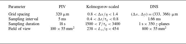

 f=4
 φ=π/2(a−d)
 φ=π(e−h)
 a,e
 ⟨u⟩/U∞
 b,f
 ⟨v⟩/U∞
 c,g
 ⟨u″2⟩/U∞
 d,h
 −⟨u″v″⟩/U∞2
 Δx/λ=1/4

 δ95

 x/λ∈[6,7]
 δ95

 a
 b
 c
 yw
 St=0.41
 St=0.62
 St=1.2

 fw=6
 λ2=−0.005

 St=0.10
 (a,b)
 ⟨u⟩/U∞
 (c,d)
 ⟨u″2⟩/U∞
 (e,f)
 −⟨u″v″⟩/U∞2
 (a,c,e)
 φ=π/2
 (b,d,f)
 φ=π

 a
 δ95/a
 x/λ=6
 St
 b
 U/U∞
 x/λ∈[6, 7]
 δ95/a

 (a)
 δ95/a
 (b)
 (δ95−δBlasius)/a

 λ2
 fw
 St=1.2
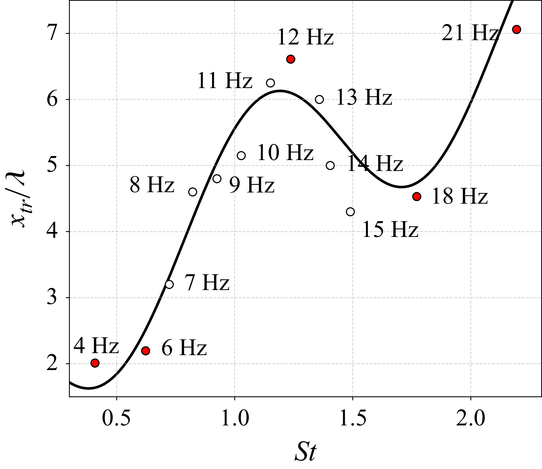
 St
 xtr
 xtr

 (a)
 (x/λ, y/a)=(2, 2.5)
 ×
 (b)
 (b)
 λ2
 St=0.62
 fw=6

 (a)
 (x/λ,y/a)=(7,2.5)
 ×
 (b)
 (b)
 λ2
 St=1.2
 fw=12
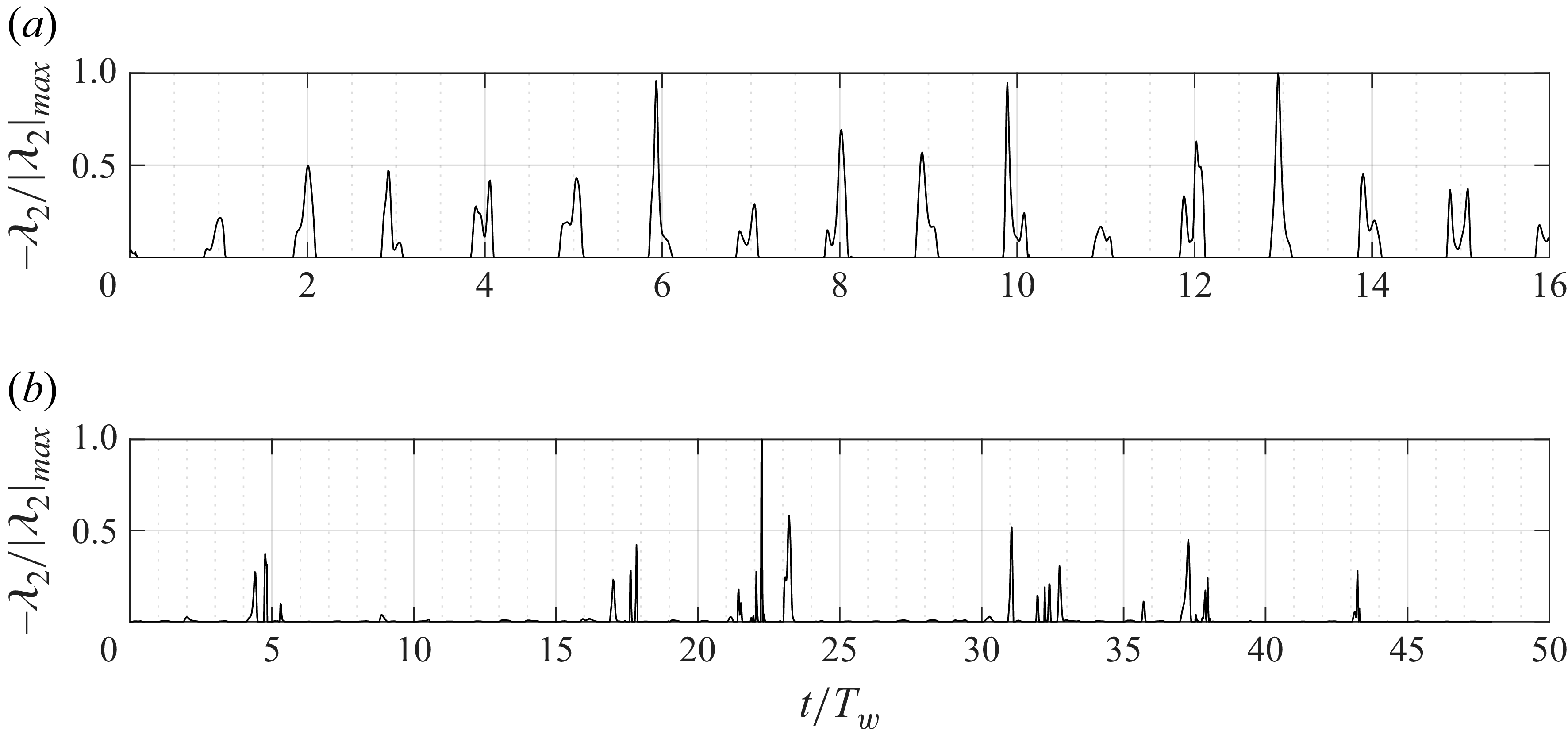
 −λ2/|λ2|max
 y/a=3
 St=0.62
 x/λ=2
 (b)
 St=1.2
 x/λ=6.5

 λ2
 y/a=3
 (a)St=0.62
 (b)St=1.2
 (a)x/λ=1
 (b)x/λ=5.5

 x/λ=6.5
 (a)
 y/a
 (b)
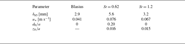
 x/λ≈7.5
 St
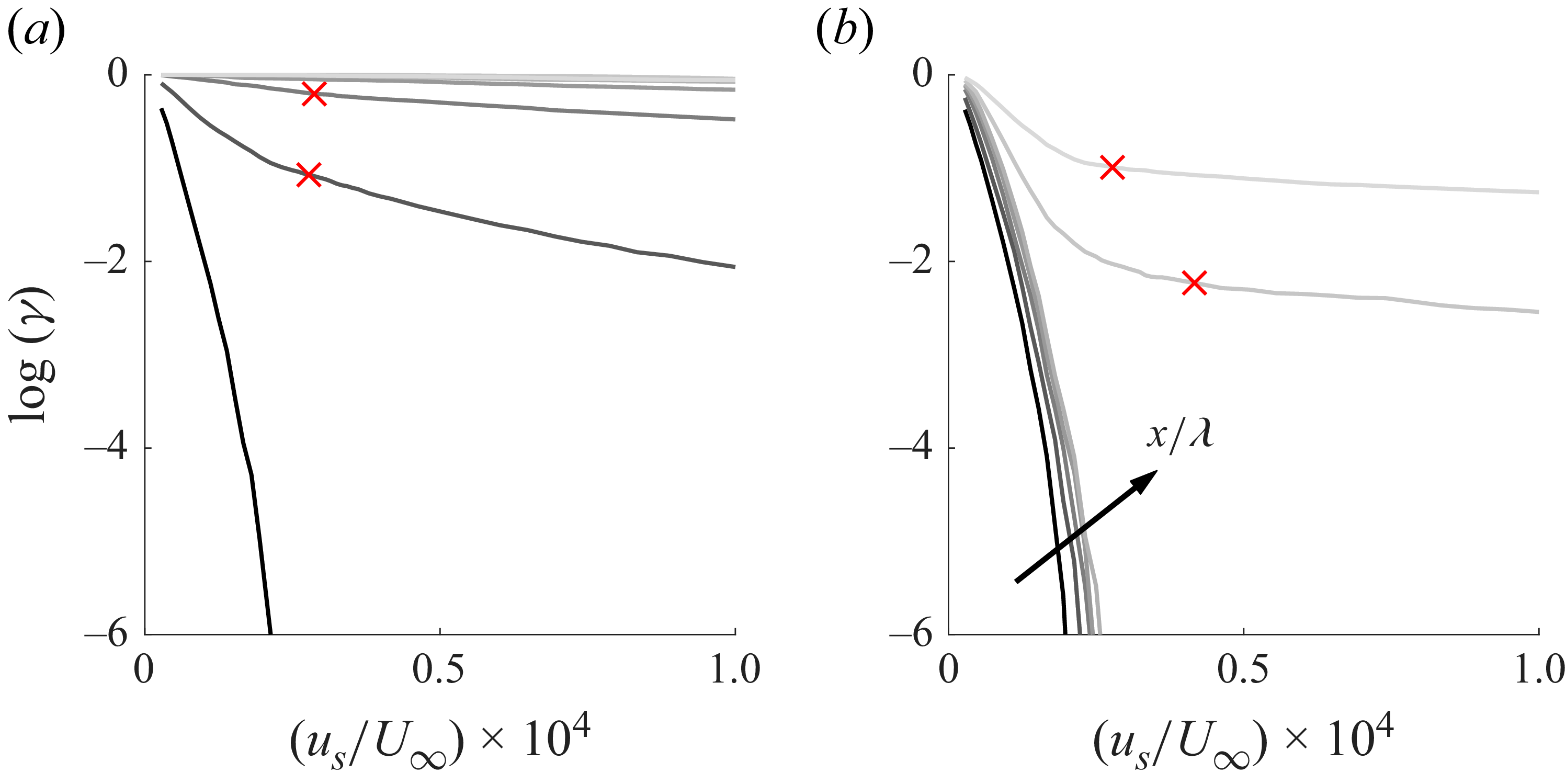
 x/λ=1
 y/a=2.5
 us∗
 (a)fw=4
 (b)


 Open access

