1 Introduction
The study of the geometry of fixed elements of automorphisms of spherical buildings is a well-established and beautiful topic (see [Reference Petersson, Mühlherr and Weiss19]). Over the past decade, a complementary theory concerning the “opposite geometry,” consisting of those elements mapped to opposite elements by an automorphism of a spherical building, has been developed. A starting point for this theory is the fundamental result of Abramenko and Brown [Reference Abramenko and Brown2, Proposition 4.2], stating that if
 $\theta $
is a nontrivial automorphism of a thick spherical building, then the opposite geometry
 $\operatorname {{\mathrm {Opp}}}(\theta )$
is necessarily nonempty. Indeed, the generic situation is that
 $\operatorname {{\mathrm {Opp}}}(\theta )$
is rather large, and typically contains many chambers of the building (chambers are the simplices of maximal dimension). The more special situation is when
 $\operatorname {{\mathrm {Opp}}}(\theta )$
contains no chamber, in which case
 $\theta $
is called domestic.
Domestic automorphisms have recently enjoyed extensive investigation (see [Reference Parkinson, Temmermans and Van Maldeghem14–Reference Parkinson and Van Maldeghem16, Reference Temmermans, Thas and Van Maldeghem24–Reference Temmermans, Thas and Van Maldeghem26, Reference Van Maldeghem31, Reference Van Maldeghem and Sastry32]). Cumulatively, these papers begin to illuminate an as yet not fully understood connection between domesticity of an automorphism, and a large rich fixed element structure of the automorphism. For example, by [Reference Van Maldeghem31], the domestic dualities of large
 $\mathsf {E}_6$
buildings are precisely the polarities that fix a split building of type
 $\mathsf {F}_4$
, and by [Reference Van Maldeghem and Sastry32], the domestic trialities of
 $\mathsf {D}_4$
buildings are precisely the automorphisms fixing a split building of type
 $\mathsf {G}_2$
. These remarkable connections underscore the importance of both the opposite geometry and the notion of domesticity in the theory of spherical buildings.
A systematic study of the opposite geometry was initiated in [Reference Parkinson and Van Maldeghem15, Reference Parkinson and Van Maldeghem16], where we developed the notion of an opposition diagram of an automorphism, encoding the types of the simplices of the building that are mapped onto opposite simplices by the automorphism. This concept gives a useful framework for the study of the opposite geometry and domesticity. Indeed, a striking consequence of the theory is that there are surprisingly few opposition diagrams possible. The purpose of this paper (along with [Reference Parkinson and Van Maldeghem17, Reference Parkinson, Van Maldeghem and Victoor18]) is to classify, as much as possible, the class of automorphisms having each opposition diagram, with the focus of this paper being on split spherical buildings of exceptional type.
Let us briefly expand on the above concepts, before summarizing our main results. Suppose that
 $\Delta $
is an irreducible split spherical building with Dynkin diagram
 $\Gamma $
. The opposition diagram
 $\operatorname {{\mathrm {Diag}}}(\theta )$
of an automorphism
 $\theta $
of
 $\Delta $
is drawn by encircling the nodes of
 $\Gamma $
corresponding to the types of the minimal simplices of
 $\Delta $
that are mapped onto opposite simplices by
 $\theta $
.
For example, the diagram
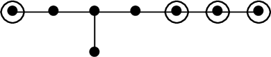
represents an automorphism of an
 $\mathsf {E}_8$
building mapping vertices of types
 $1,6,7,$
and
 $8$
, and no vertices of other types, to opposite vertices (we adopt Bourbaki labeling [Reference Bourbaki4]). A priori, there could be
 $2^8$
possible opposition diagrams for automorphisms of
 $\mathsf {E}_8$
buildings; however, it is a remarkable fact that there are only five diagrams possible. The idea behind the proof of this fact, from [Reference Parkinson and Van Maldeghem15, Reference Parkinson and Van Maldeghem16], is as follows. Suppose first that
 $\Delta $
is a large spherical building of rank at least
 $3$
(meaning that
 $\Delta $
has no Fano plane residues). In [Reference Parkinson and Van Maldeghem15, Theorem 1], we showed that every automorphism
 $\theta $
of
 $\Delta $
satisfies the following closure property: If there exist type
 $J_1$
and
 $J_2$
simplices in
 $\operatorname {{\mathrm {Opp}}}(\theta )$
, then there exists a type
 $J_1\cup J_2$
simplex in
 $\operatorname {{\mathrm {Opp}}}(\theta )$
. Such automorphisms are called capped, and this highly nontrivial property imposes severe constraints on the structure of opposition diagrams. For small spherical buildings, it turns out that automorphisms are not necessarily capped; however, the same constraints on the opposition diagrams exist for other reasons (see [Reference Parkinson and Van Maldeghem16]).
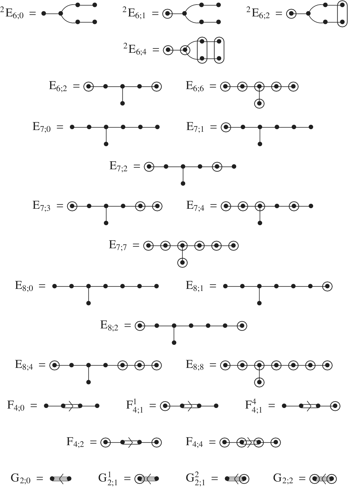
We call a diagram satisfying the constraints imposed by cappedness an admissible diagram. The precise constraints are not required here (see [Reference Parkinson and Van Maldeghem15, Section 2.1] for details), as it is sufficient for our purpose to simply give the complete list of admissible Dynkin diagrams of exceptional type, see Figure 1.
To summarize, if
 $\theta $
is an automorphism of a split spherical building of exceptional type, then the opposition diagram of
 $\theta $
is one of the diagrams listed in Figure 1. Uncapped automorphisms are studied in [Reference Parkinson and Van Maldeghem16], and so for, the remainder of this introduction we consider capped automorphisms (for example, if
 $\Delta $
is large, then all automorphisms are capped). In this case, automorphisms with “full” opposition diagrams (in which all nodes are encircled) are necessarily not domestic, and hence are not discussed further here. Moreover, the “empty” diagrams with no nodes encircled correspond precisely to the trivial automorphisms (because as mentioned above,
 $\operatorname {{\mathrm {Opp}}}(\theta )$
is nonempty for a nontrivial automorphism), and hence are also of little interest here. Furthermore, automorphisms with diagram
 $\mathsf {E}_{6;2}$
have been completely classified in [Reference Van Maldeghem and Sastry32] (for large buildings) and [Reference Parkinson and Van Maldeghem16] (for small buildings). This leaves us with
 $14$
remaining diagrams.
The admissible Dynkin diagrams of exceptional type.
The following terms will be defined more systematically in latter sections; however, for the purpose of this introduction, and in order to state our main results, we define:
-
(1) The polar diagrams to be the diagrams
 ${^2}\mathsf {E}_{6;1},\mathsf {E}_{7;1},\mathsf {E}_{8;1},\mathsf {F}_{4;1}^1,\mathsf {G}_{2;1}^2$
;
-
(2) The polar–copolar diagrams to be the diagrams
${^2}\mathsf {E}_{6;2}$
,
$\mathsf {E}_{7;2}$
,
$\mathsf {E}_{8;2}$
,
$\mathsf {F}_{4;2}$
; -
(3) The polar closed diagrams to be all diagrams except
$\mathsf {E}_{6;2},\mathsf {E}_{6;6},\mathsf {F}_{4;1}^4,\mathsf {G}_{2;1}^1$
.




We consider split spherical buildings arising from a Chevalley group
 $G=G_{\Phi }(\mathbb {F})$
associated to a crystallographic root system
 $\Phi $
, with
 $\mathbb {F}$
a field. For the purpose of this introduction, unless stated explicitly otherwise, we will assume that the characteristic of
 $\mathbb {F}$
is not “special” (meaning
 $\mathrm {char}(\mathbb {F})\neq 2$
for
 $\mathsf {F}_4$
, and
 $\mathrm {char}(\mathbb {F})\neq 3$
for
 $\mathsf {G}_2$
). By a root elation, we mean an element, in Chevalley generators, conjugate to
 $x_{\alpha }(a)$
for some root
 $\alpha \in \Phi $
and some
 $a\neq 0$
. In the nonsimply laced case, we talk of long and short root elations, and in the simply laced case, all roots are considered long. Root elations
 $x_{\alpha }(a)$
and
 $x_{\beta }(b)$
are perpendicular if
 $\alpha $
and
 $\beta $
are perpendicular roots. A positive root elation is an element
 $x_{\alpha }(a)$
with
 $\alpha \in \Phi ^+$
, where
 $\Phi ^+$
is a fixed choice of positive roots of
 $\Phi $
. By a homology, we mean an element conjugate to an element of the torus H.
With these definitions and conventions, a summary of the main results of this paper is as follows. We first give a complete classification of automorphisms with polar opposition diagram.
Theorem 1 An automorphism of a split spherical building of exceptional type has polar opposition diagram if and only if it is a long root elation.
In fact, some aspects of our analysis of long root elations apply to all Moufang spherical buildings, and lead to various corollaries, including the following.
Corollary 2 Every irreducible Moufang spherical building, other than a projective plane, admits a nontrivial domestic collineation.
Corollary 3 Let G be the collineation group of a Moufang spherical building
 $\Delta $
of type other than
 $\mathsf {A}_n$
. There exists a nontrivial conjugacy class
 $\mathscr {C}$
in G which is not transitive on the set of vertices of
 $\Delta $
of type s, for any
 $s\in S$
.
In the case of Ree–Tits octagons, Corollary 2 corrects a misunderstanding from [Reference Ihringer, Sin and Xiang11] (see Remark 3.3), and Corollary 3 answers a question asked to us by Barbara Baumeister.
The classification of automorphisms with polar opposition diagram can be extended to the polar–copolar diagrams in certain cases. We prove the following theorem.
Theorem 4 A collineation of a large split spherical building of type
 $\mathsf {E}_7$
,
 $\mathsf {E}_8$
, or
 $\mathsf {F}_4$
has polar–copolar opposition diagram if and only if it is a product of two perpendicular long root elations. Moreover, for the
 $\mathsf {E}_7$
and
 $\mathsf {E}_8$
cases, the collineations with polar–copolar diagram form a single conjugacy class.
See Theorem 7 below for more details on the conjugacy classes in type
 $\mathsf {F}_4$
. In addition, we note that the “if” part of Theorem 4 holds for the
 $\mathsf {E}_{6}$
case too; however, the “only if” part fails, as there exist homologies with diagram
 ${^2}\mathsf {E}_{6;2}$
(see Theorems 6 and 8 below).
Our next main theorem classifies the opposition diagrams of elements of the unipotent subgroup
 $U^+$
generated by the positive root elations.
Theorem 5 Let
 $\Delta $
be a split spherical building with root system
 $\Phi $
of exceptional type. An admissible Dynkin diagram
 $\mathsf {X}$
of type
 $\Phi $
can be obtained as the opposition diagram of a product of positive root elations of
 $\Delta $
if and only if
 $\mathsf {X}$
is polar closed.
Moreover, we provide an algorithm to write down, for each polar closed diagram
 $\mathsf {X}$
, an element
 $\theta \in U^+$
with opposition diagram
 $\mathsf {X}$
. In fact, it turns out that every polar closed diagram can be obtained as the opposition diagram of a product of mutually perpendicular positive root elations.
Next, we give a complete classification of domestic homologies for split exceptional buildings. This classification is in terms of the type of the thick frame of the fixed subbuilding of the automorphism (cf. [Reference Scharlau20]). We summarize the statement below (see Section 5 for explicit conjugacy class representatives for each case).
Theorem 6 Let
 $\theta $
be a nontrivial homology of a split spherical building of exceptional type
 $\Phi $
, and let
 $\Phi '$
be the type of the thick frame of the subbuilding fixed by
 $\theta $
. Then,
 $\theta $
is domestic if and only if:
-
(1)
$\Phi =\mathsf {E}_6$
and
$\Phi '=\mathsf {D}_5$
, in which case
$\operatorname {{\mathrm {Diag}}}(\theta )={^2}\mathsf {E}_{6;2}$
; -
(2)
$\Phi =\mathsf {E}_7$
and
$\Phi '=\mathsf {E}_6, \mathsf {D}_6,\mathsf {D}_6\times \mathsf {A}_1$
, in which case
$\operatorname {{\mathrm {Diag}}}(\theta )=\mathsf {E}_{7;3},\mathsf {E}_{7;4},\mathsf {E}_{7;4}$
(respectively); -
(3)
$\Phi =\mathsf {E}_8$
and
$\Phi '=\mathsf {E}_7,\mathsf {E}_7\times \mathsf {A}_1$
, in which case
$\operatorname {{\mathrm {Diag}}}(\theta )=\mathsf {E}_{8;4}$
; -
(4)
$\Phi =\mathsf {F}_4$
and
$\Phi '=\mathsf {B}_4$
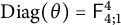
, in which case
$\operatorname {{\mathrm {Diag}}}(\theta )=\mathsf {F}_{4;1}^4$
; -
(5)
$\Phi =\mathsf {G}_2$
and
$\Phi '=\mathsf {A}_2$
, in which case
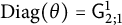
$\operatorname {{\mathrm {Diag}}}(\theta )=\mathsf {G}_{2;1}^1$
.













We also completely classify domestic automorphisms of split buildings of types
 $\mathsf {E}_6$
,
 $\mathsf {F}_4$
, and
 $\mathsf {G}_2$
. For this introduction, let us state the result for
 $\mathsf {F}_4$
over quadratically closed fields and finite fields, both of characteristic not
 $2$
(see Section 7.1 for statements applying to all fields).
Theorem 7 Let
 $\Delta $
be the split spherical building of
 $G=\mathsf {F}_4(\mathbb {F})$
with
 $\mathrm {char}(\mathbb {F})\neq 2$
. If
 $\ \mathbb {F}$
is quadratically closed (respectively finite), then there are precisely three (respectively four) conjugacy classes of domestic collineations, consisting of:
-
(1) the class of long root elations, with opposition diagram
$\mathsf {F}_{4;1}^1$
; -
(2) the class of homologies fixing a subbuilding with thick frame of type
$\mathsf {B}_4$
, with opposition diagram
$\mathsf {F}_{4;1}^4$
; -
(3) one (respectively two) class(es) of products of two perpendicular long root elations, with opposition diagram
$\mathsf {F}_{4;2}$
.


For the
 $\mathsf {E}_6$
case, domestic automorphisms of small buildings are already classified in [Reference Parkinson and Van Maldeghem16, Theorems 4.5 and 4.6], and domestic dualities of large buildings are classified in [Reference Van Maldeghem and Sastry32]. Thus, by Theorem 1 and the classification of admissible diagrams, the remaining task is to classify the collineations of large
 $\mathsf {E}_6$
buildings with diagram
 ${^2}\mathsf {E}_{6;2}$
. It turns out that the only examples are those described by Theorems 5 and 6, and thus we have the following theorem.
Theorem 8 Let
 $\Delta $
be a large building of type
 $\mathsf {E}_6$
.
-
(1) A duality of
$\Delta $
is domestic if and only if it is a symplectic polarity (that is, a duality fixing a split building of type
$\mathsf {F}_4$
), in which case it has opposition diagram
$\mathsf {E}_{6;2}$
. -
(2) A collineation of
$\Delta $
is domestic if and only if it is either:-
(a) a root elation, with opposition diagram
${^2}\mathsf {E}_{6;1}$
, -
(b) a product of two perpendicular root elations, with opposition diagram
${^2}\mathsf {E}_{6;2}$
, or -
(c) a homology fixing a subbuilding with thick frame of type
$\mathsf {D}_5$
, with opposition diagram
${^2}\mathsf {E}_{6;2}$
.
-


We complete the analysis by classifying domestic automorphisms of split
 $\mathsf {G}_2$
buildings. Because no duality of a
 $\mathsf {G}_2$
building is domestic [Reference Parkinson, Temmermans and Van Maldeghem14, Theorem 2.7], it suffices to consider collineations.
Theorem 9 Let
 $\Delta $
be the building of
 $\mathsf {G}_2(\mathbb {F})$
. There exists a unique conjugacy class
 $\mathscr {C}_1$
of collineations with opposition diagram
 $\mathsf {G}_{2;1}^2$
, and a unique conjugacy class
 $\mathscr {C}_2$
of collineations with opposition diagram
 $\mathsf {G}_{2;1}^1$
. The elements of
 $\mathscr {C}_1$
are long root elations, and the elements of
 $\mathscr {C}_2$
:
-
(1) are short root elations if
$\mathrm {char}(\mathbb {F})=3$
; -
(2) are homologies fixing a large full subhexagon if
$\mathrm {char}(\mathbb {F})\neq 3$
and
$z^2+z+1$
splits over
$\mathbb {F}$
; -
(3) fix a distance
$3$
-ovoid if
$z^2+z+1$
is irreducible over
$\mathbb {F}$
.


Consequently, the results of this paper (along with [Reference Van Maldeghem and Sastry32] for the
 $\mathsf {E}_{6;2}$
diagram) culminate in the classification of automorphisms of split spherical buildings of exceptional type having each nonfull opposition diagram, with the exception of the three diagrams
 $\mathsf {E}_{7;3}$
,
 $\mathsf {E}_{7;4}$
, and
 $\mathsf {E}_{8;4}$
. In these remaining cases, we have provided examples of both unipotent elements and homologies with the given diagram (in Theorems 5 and 6). It turns out that for certain fields, there also exist automorphisms with these opposition diagrams fixing no chamber of the building (hence, these automorphisms are neither unipotent elements nor homologies). The description and classification of these automorphisms will be continued in future work [Reference Parkinson, Van Maldeghem and Victoor18].
We note that the results of this paper, combined with those of [Reference Parkinson and Van Maldeghem17] for the classical cases, show that every admissible Dynkin diagram can be obtained as the opposition diagram of an automorphism of a split spherical building. As discussed in [Reference Parkinson and Van Maldeghem17], this statement is false for certain no-split buildings. More precisely, we have the following corollary.
Corollary 10 Let
 $\Delta $
be a split spherical building of type
 $\Phi $
. Every admissible Dynkin diagram of type
 $\Phi $
is the opposition diagram of some automorphism of
 $\Delta $
. Moreover, with only one exception, such an automorphism can be chosen such that it fixes a chamber of the building. This exception is the diagram
 $\mathsf {G}_{2;1}^1$
in the case that the polynomial
 $z^2+z+1$
is irreducible over the underlying field
 $\mathbb {F}$
.
Finally, our results translate into group theoretic statements concerning conjugacy classes in Chevalley groups of exceptional type. To put these results into context, recall that by the Density Theorem (see [Reference Humphreys10, Section 22.2]), if G is a connected linear algebraic group over an algebraically closed field, then the union of all conjugates of a Borel subgroup B is equal to G. Equivalently, if
 $\mathscr {C}$
is a conjugacy class in G, then
 $\mathscr {C}\cap B\neq \emptyset $
. This theorem is a cornerstone in the theory of algebraic groups; for example, simple corollaries include the important facts that the centers of G and B coincide, and that the Cartan subgroups of G are precisely the centralizers of maximal tori.
The statement of the Density Theorem is clearly false in the general setting of a Chevalley group G over an arbitrary field, as there typically exist elements
 $\theta \in G$
fixing no chamber of the building
 $\Delta =G/B$
. However, our classification theorems allow us to provide analogues in this setting, showing that every conjugacy class in G intersects a union of a very small number of B-double cosets. For the purpose of this introduction, we provide two examples; see Section 7.4 for further related statements.
Corollary 11 Let G be the Chevalley group of type
 $\mathsf {E}_6$
or
 $\mathsf {F}_4$
over a field
 $\mathbb {F}$
, and let
 $\mathscr {C}$
be a conjugacy class in G. Then,
 $\mathscr {C}\cap (B\cup Bw_0B)\neq \emptyset $
.
The statement of Corollary 11 fails for buildings of types
 $\mathsf {E}_7$
and
 $\mathsf {E}_8$
(see Remark 7.16). Moreover, it is not true that
 $\mathscr {C}\cap Bw_0B\neq \emptyset $
for all nontrivial conjugacy classes. In fact, we have the following very general corollary of our results.
Corollary 12 Let G be the group of type preserving automorphisms of a Moufang spherical building not of type
 $\mathsf {A}_2$
. There exists a nontrivial conjugacy class
 $\mathscr {C}$
with
 $\mathscr {C}\cap Bw_0B= \emptyset $
.
Let us conclude this introduction with an outline of the structure of the paper. In Section 2, we provide background on buildings, Chevalley groups, and admissible diagrams, and prove some basic lemmas for latter use. In Section 3, we give the classification of automorphisms of split buildings with polar opposition diagram, proving Theorem 1 and Corollaries 2 and 3. Most of the arguments of this section are built around commutator relations in the Chevalley group, and we also discuss geometric characterizations of the polar diagram in the
 $\mathsf {E}_{6,1}$
and
 $\mathsf {E}_{7,7}$
Lie incidence geometries, and analyze short root elations in the nonsimply laced case.
In Section 4, we define polar closed diagrams, and present an algorithm for constructing unipotent elements with each polar closed diagram (proving Theorem 5). Most of the arguments here are algebraic; however, to complete the proof, it is necessary to show that automorphisms with diagram
 $\mathsf {F}_{4,1}^4$
are necessarily homologies (for
 $\mathrm {char}(\mathbb {F})\neq 2$
), and we achieve this by arguing geometrically in the Lie incidence geometry
 $\mathsf {F}_{4,4}(\mathbb {F})$
.
Section 5 gives the complete classification of domestic homologies for split exceptional buildings (proving Theorem 6), making use of Scharlau’s classification [Reference Scharlau20] of nonthick spherical buildings. In Section 6, we prove Theorem 4 using geometric arguments involving various Lie incidence geometries.
Finally, in Section 7, we provide the complete classification of domestic collineations for split buildings of types
 $\mathsf {E}_6$
,
 $\mathsf {F}_4$
, and
 $\mathsf {G}_2$
, proving Theorems 7, 8, and 9, and Corollaries 10, 11, and 12. We conclude with an append ix listing some relevant root system data for exceptional types. These data are useful at various stages of this paper, for example, when performing commutator relations, or, in Section 5, when classifying domestic homologies.
2 Background and definitions
In this section, we give a brief account of root systems, Chevalley groups, and split spherical buildings, with our main references being [Reference Bourbaki4, Reference Carter5, Reference Steinberg23] (for root systems and Chevalley groups) and [Reference Abramenko and Brown1, Reference Tits28] (for buildings). We also recall the notions of admissible diagrams and opposition diagrams from [Reference Parkinson and Van Maldeghem15, Reference Parkinson and Van Maldeghem16], and record some basic lemmas for latter use.
2.1 Root systems and Chevalley groups
Let
 $\Phi $
be a reduced irreducible crystallographic root system in an n-dimensional real vector space V with inner product
 $\langle \cdot ,\cdot \rangle $
, with
 $\alpha _1,\ldots ,\alpha _n$
a choice of simple roots and
 $\Phi ^+$
the associated positive roots. We will adopt the standard Bourbaki labeling [Reference Bourbaki4] of the simple roots. Let
 $\alpha ^{\vee }=2\alpha /\langle \alpha ,\alpha \rangle $
. Let
 $\omega _1,\ldots ,\omega _n$
be the fundamental coweights, defined by
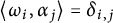 $\langle \omega _i,\alpha _j\rangle =\delta _{i,j}$
. Let
 $$ \begin{align*}Q=\mathbb{Z}\alpha_1^{\vee}+\cdots+\mathbb{Z}\alpha_n^{\vee}\quad\text{and}\quad P=\mathbb{Z}\omega_1+\cdots+\mathbb{Z}\omega_n \end{align*} $$
be the coroot lattice and coweight lattice, respectively, and note that
 $Q\subseteq P$
.
Let
 $\Gamma =\Gamma (\Phi )$
denote the Dynkin diagram of
 $\Phi $
(with the arrow pointing toward the short root in the case of double and triple bonds). The Coxeter diagram of
 $\Phi $
is obtained by removing all arrows from
 $\Gamma $
. The height of a root
 $\alpha =k_1\alpha _1+\cdots +k_n\alpha _n$
is
 $\mathrm {ht}(\alpha )=k_1+\cdots +k_n$
. There is a unique root
 $\varphi \in \Phi $
of maximal height (the highest root of
 $\Phi $
). The polar type of
 $\Phi $
is the subset
 $\wp \subseteq \{1,2,\ldots ,n\}$
given by
 $$ \begin{align*}\wp=\{1\leq i\leq n\mid \langle\alpha_i,\varphi\rangle\neq0\}. \end{align*} $$
See Appendix A for the list of polar types. In particular, note that if
 $\Phi \neq \mathsf {A}_n$
, then
 $\wp =\{p\}$
is a singleton set, and in this case, we often refer to the element p as the polar node.
Let
 $W=\langle s_{\alpha }\mid \alpha \in \Phi \rangle $
be the subgroup of
 $\mathsf {GL}(V)$
generated by the reflections
 $s_{\alpha }$
, where
 $$ \begin{align*}s_{\alpha}(\lambda)=\lambda-\langle\lambda,\alpha\rangle\alpha^{\vee}\quad\text{for}\ \lambda\in V. \end{align*} $$
Let
 $S=\{s_1,\ldots ,s_n\}$
, where
 $s_i=s_{\alpha _i}$
. Then,
 $(W,S)$
is a spherical Coxeter system. Writing
 $\ell : W\to \mathbb {Z}_{\geq 0}$
for the usual length function on W, it is a well-known fact that in the simply laced case,
 $\ell (s_{\alpha })=2\mathrm {ht}(\alpha )-1$
.
Let
 $w_0$
denote the longest element of
 $(W,S)$
, and let
 $\pi _0:\{1,\ldots ,n\}\to \{1,\ldots ,n\}$
be the opposition relation given by
 $w_0\alpha _i=-\alpha _{\pi _0(i)}$
, for
 $1\leq i\leq n$
. We typically regard
 $\pi _0$
as an automorphism of the Dynkin diagram
 $\Gamma $
, and we say that “opposition is type preserving” if
 $\pi _0$
is the identity. If
 $J\subseteq S$
, let
 $w_J$
be the longest element of the parabolic subgroup
 $W_J$
generated by J.
The inversion set of
 $w\in W$
is
 $ \Phi (w)=\{\alpha \in \Phi ^+\mid w^{-1}\alpha \in -\Phi ^+\}. $
We note that the inversion set of the highest root
 $\varphi $
is
 $$ \begin{align} \Phi(s_{\varphi})=\{\alpha\in\Phi^+\mid \langle\alpha,\omega_i\rangle>0\text{ for some}\ i\in\wp\}, \end{align} $$
which follows directly from the equation
 $s_{\varphi }(\alpha )=\alpha -\langle \alpha ,\varphi ^{\vee }\rangle \varphi $
.
Let
 $\mathbb {F}$
be a field, and let
 $G_0=G_0(\Phi ,\mathbb {F})$
be the associated adjoint Chevalley group. Thus,
 $G_0$
is generated by elements
 $x_{\alpha }(a)$
with
 $\alpha \in \Phi $
and
 $a\in \mathbb {F}$
, and writing (for
 $\alpha \in \Phi $
and
 $c\in \mathbb {F}^{\times }$
)
 $$ \begin{align*} s_{\alpha}(c)=x_{\alpha}(c)x_{-\alpha}(-c^{-1})x_{\alpha}(c)\quad\text{and}\quad h_{\alpha^{\vee}}(c)=s_{\alpha}(c)s_{\alpha}(1)^{-1}, \end{align*} $$
the following relations hold (for
 $a,b\in \mathbb {F}$
,
 $\alpha ,\beta \in \Phi $
with
 $\beta \neq \pm \alpha $
, and
 $c,d\in \mathbb {F}^{\times }$
)
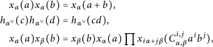 $$ \begin{align*} x_{\alpha}(a)x_{\alpha}(b)&=x_{\alpha}(a+b),\\ h_{\alpha^{\vee}}(c)h_{\alpha^{\vee}}(d)&=h_{\alpha^{\vee}}(cd),\\ x_{\alpha}(a)x_{\beta}(b)&=x_{\beta}(b)x_{\alpha}(a)\prod x_{i\alpha+j\beta}(C_{\alpha,\beta}^{i,j}a^ib^j), \end{align*} $$
where the product is taken over
 $i,j\geq 1$
with
 $i\alpha +j\beta \in \Phi $
in any fixed order, and the elements
 $C_{\alpha ,\beta }^{i,j}$
are integers (depending on the order chosen in the product). For example, in the simply laced case, these commutator relations take the form
 $x_{\alpha }(a)x_{\beta }(b)=x_{\beta }(b)x_{\alpha }(a)$
(if
 $\alpha +\beta \notin \Phi $
) or
 $x_{\alpha }(a)x_{\beta }(b)=x_{\beta }(b)x_{\alpha }(a)x_{\alpha +\beta }(C_{\alpha ,\beta }ab)$
for some integer
 $C_{\alpha ,\beta }$
(if
 $\alpha +\beta \in \Phi $
), and it turns out that in this case
 $C_{\alpha ,\beta }=\pm 1$
.
The above relations imply the following useful formula (for
 $\alpha ,\beta \in \Phi $
and
 $a\in \mathbb {F}$
):
 $$ \begin{align*} s_{\alpha}(1)x_{\beta}(a)s_{\alpha}(1)^{-1}=x_{s_{\alpha}\beta}(\epsilon_{\alpha\beta}a), \end{align*} $$
where
 $\epsilon _{\alpha \beta }=\pm 1$
depend on some initial choices made in the Lie algebra (see [Reference Carter5, Proposition 4.2.2]). For many calculations, it is sufficient to simply know that
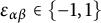 $\epsilon _{\alpha \beta }\in \{-1,1\}$
; however, when more precise knowledge is required, we will adopt the sign conventions from the Groups of Lie Type package in Magma [Reference Bosma, Cannon and Playoust3, Reference Cohen, Murray and Taylor6].
Let
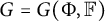 $G=G(\Phi ,\mathbb {F})$
be the subgroup of
 $\mathrm {Aut}(G_0)$
generated by the inner automorphisms
 $G_0$
and the diagonal automorphisms, as in [Reference Humphreys8, Reference Steinberg22]. Thus, G is generated by
 $G_0$
and elements
 $h_{\lambda }(c)$
with
 $\lambda \in P$
and
 $c\in \mathbb {F}^{\times }$
, and the following relations hold (for
 $a\in \mathbb {F}$
,
 $c,d\in \mathbb {F}^{\times }$
,
 $\alpha ,\beta \in \Phi $
, and
 $\lambda ,\mu \in P$
):
 $$ \begin{align*} h_{\lambda}(c)h_{\mu}(d)&=h_{\mu}(c)h_{\lambda}(d)& h_{\lambda}(c)h_{\lambda}(d)&=h_{\lambda}(cd),\\ h_{\lambda}(c)x_{\alpha}(a)h_{\lambda}(c)^{-1}&=x_{\alpha}(ac^{\langle\lambda,\alpha\rangle})&s_{\alpha}(1)h_{\lambda}(d)s_{\alpha}(1)^{-1}&=h_{s_{\alpha}\lambda}(d). \end{align*} $$
For each
 $\alpha \in \Phi $
, we write
 $U_{\alpha }=\langle x_{\alpha }(a)\mid a\in \mathbb {F}\rangle $
and
 $U^+=\langle U_{\alpha }\mid \alpha \in \Phi ^+\rangle $
. Let
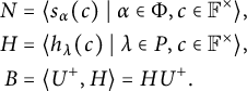 $$ \begin{align*} N&=\langle s_{\alpha}(c)\mid \alpha\in\Phi, c\in\mathbb{F}^{\times}\rangle,\\ H&=\langle h_{\lambda}(c)\mid \lambda\in P,c\in\mathbb{F}^{\times}\rangle,\\ B&=\langle U^+,H\rangle=HU^+. \end{align*} $$
The subgroup B is often called the (standard) Borel subgroup. We have
 $H=B\cap N$
, and
 $(B,N)$
is a
 $BN$
-pair in G with Weyl group
 $N/H\cong W$
, where
 $$ \begin{align*}s_{\alpha}(c)H\mapsto s_{\alpha}\quad\text{for all}\ c\in \mathbb{F}^{\times}. \end{align*} $$
We often write
 $wH$
(or
 $wB$
) in place of
 $nH$
(or
 $nB$
) whenever
 $n\in N$
with
 $nH\mapsto w$
. In fact, we will frequently write
 $s_{\alpha }$
in place of
 $s_{\alpha }(1)$
when there is no risk of confusion; however, note that
 $s_{\alpha }\in G$
is typically not an involution.
The Bruhat decomposition gives
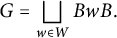 $$ \begin{align*}G=\bigsqcup_{w\in W}BwB. \end{align*} $$
For subsets
 $A\subseteq \Phi ^+$
, we write
 $U_A^+=\langle x_{\alpha }(a)\mid \alpha \in A,\,a\in \mathbb {F}\rangle $
. A subset
 $A\subseteq \Phi ^+$
is closed if
 $\alpha ,\beta \in A$
and
 $\alpha +\beta \in \Phi $
implies that
 $\alpha +\beta \in A$
. It is a fundamental fact that if
 $A\subseteq \Phi ^+$
is closed, and if
 $(\beta _1,\ldots ,\beta _k)$
is a fixed choice of ordering of the elements of A, then each
 $u\in U_A^+$
has a unique expression as
 $ u=x_{\beta _1}(a_1)\cdots x_{\beta _k}(a_k) $
for some
 $a_1,\ldots ,a_k\in \mathbb {F}$
(see [Reference Steinberg23, Lemma 17]). In particular, because the set
 $A=\Phi (w)$
is closed, the B cosets in
 $BwB$
are precisely
 $$ \begin{align} x_{\beta_1}(a_1)\cdots x_{\beta_k}(a_k)wB,\quad\text{with}\ a_1,\ldots,a_k\in\mathbb{F}, \end{align} $$
where
 $\Phi (w)=\{\beta _1,\ldots ,\beta _k\}$
.
We also note that
 $$ \begin{align} BwB\cdot BsB&=\begin{cases} BwsB&\text{if}\ \ell(ws)=\ell(w)+1\\ BwB\cup BwsB&\text{if}\ \ell(ws)=\ell(w)-1 \end{cases} \end{align} $$
(see [Reference Carter5, Proposition 8.1.5]).
Let
 $U^-=\langle U_{\alpha }\mid \alpha \in -\Phi ^+\rangle $
. Throughout this paper, we often need to convert an element in
 $U^-$
to an expression in
 $BwB$
for some w. To do so, we make frequent use of the relation (for
 $a\neq 0$
)
 $$ \begin{align} x_{-\alpha}(a)=x_{\alpha}(a^{-1})s_{\alpha}(-a^{-1})x_{\alpha}(a^{-1})=x_{\alpha}(a^{-1})s_{\alpha}x_{\alpha}(a)h_{\alpha^{\vee}}(-a) \end{align} $$
(which follows from the definition of
 $s_{\alpha }(a)$
). We call this the folding relation, due to connections with path models in algebraic combinatorics (see [Reference Parkinson, Ram and Schwer13]).
We say that
 $\mathbb {F}$
has “special characteristic” if
 $\mathrm {char}(\mathbb {F})=2$
for
 $\Phi =\mathsf {B}_n,\mathsf {C}_n,\mathsf {F}_4$
, or
 $\mathrm {char}(\mathbb {F})=3$
for
 $\Phi =\mathsf {G}_2$
. Often these cases behave differently due to additional symmetries being present.
We record some basic lemmas for latter use.
Lemma 2.1 Let
 $\beta _1,\ldots ,\beta _N\in \Phi ^+$
be mutually perpendicular roots. Then,
 $$ \begin{align*} x_{-\beta_1}(a_1)\cdots x_{-\beta_N}(a_N)\in Bs_{\beta_1}\cdots s_{\beta_N}B\quad\text{for all}\ a_1,\ldots,a_N\neq 0. \end{align*} $$
Proof Let
 $U_k^+=\langle U_{\beta _1},\ldots ,U_{\beta _k}\rangle $
, for
 $1\leq k\leq N$
. We show, by induction, that
 $$ \begin{align*}x_{-\beta_1}(a_1)\cdots x_{-\beta_N}(a_N)\in U_N^+s_{\beta_1}\cdots s_{\beta_N}U_N^+H.\end{align*} $$
The case
 $N=1$
is the folding relation (2.4). By the induction hypothesis, and the folding relation, for
 $k>1$
, we have
 $$ \begin{align*} x_{\beta_1}(a_1)\cdots x_{\beta_{k}}(a_{k})&=us_{\beta_1}\cdots s_{\beta_{k-1}}u'h\cdot x_{\beta_k}(a_k^{-1})s_{\beta_k}x_{\beta_k}(a_k)h_{\beta_k^{\vee}}(-a_k), \end{align*} $$
for some
 $u,u'\in U_{k-1}^+$
,
 $h\in H$
. Because
 $h x_{\beta _k}(a_k^{-1})s_{\beta _k}x_{\beta _k}(a_k)=x_{\beta _k}(a)s_{\beta _k}x_{\beta _k}(b)h$
for some
 $a,b\in \mathbb {F}$
and
 $s_{\beta _1}\cdots s_{\beta _{k-1}}u'x_{\beta _k}(a)=x_{\beta _k}(\pm a)s_{\beta _1}\cdots s_{\beta _{k-1}}u'$
(as
 $\beta _k$
is orthogonal to
 $\beta _1,\ldots ,\beta _{k-1}$
), we have
 $$ \begin{align*}x_{\beta_1}(a_1)\cdots x_{\beta_{k}}(a_{k})=ux_{\beta_k}(\pm a)s_{\beta_1}\cdots s_{\beta_{k-1}}u'\cdot s_{\beta_k}x_{\beta_k}(b)hh_{\beta_k^{\vee}}(-a_k).\end{align*} $$
Similarly,
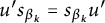 $u's_{\beta _k}=s_{\beta _k}u'$
, and hence the result.▪
Lemma 2.2 Let
 $\Phi $
have rank n, and suppose that the opposition relation is type preserving. If
 $\beta _1,\ldots ,\beta _n\in \Phi ^+$
are mutually perpendicular roots, then
 $s_{\beta _1}\cdots s_{\beta _n}=w_0$
.
Proof Because
 $\beta _1,\ldots ,\beta _n$
are mutually perpendicular, the product
 $s_{\beta _1}\cdots s_{\beta _n}$
acts by
 $-1$
on the vector space V. Because opposition is type preserving, the longest element
 $w_0$
also acts by
 $-1$
(mapping
 $\alpha _i$
to
 $-\alpha _i$
for all simple roots), and hence the result.▪
Lemma 2.3 Let
 $\Phi $
be a root system of type
 $\mathsf {E}_6$
in a vector space V, and let
 $\sigma :V\to V$
be the involution with
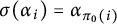 $\sigma (\alpha _i)=\alpha _{\pi _0(i)}$
, for
 $1\leq i\leq 6$
. Suppose that
 $\beta _1,\beta _2,\beta _3,\beta _4\in \Phi ^+$
are mutually perpendicular roots with
 $\sigma (\beta _i)=\beta _i$
, for
 $i=1,2,3,4$
. Then,
 $s_{\beta _1}s_{\beta _2}s_{\beta _3}s_{\beta _4}=w_0$
.
Proof Let
 $w=s_{\beta _1}s_{\beta _2}s_{\beta _3}s_{\beta _4}$
. Let
 $V'=\{v\in V\mid \sigma (v)=v\}$
. Then,
 $V'$
is four-dimensional, and because
 $\beta _1,\beta _2,\beta _3,\beta _4\in V'$
are mutually perpendicular, we have
 $s_{\beta _1}\cdots s_{\beta _4}|_{V'}=-1$
. In particular,
 $\alpha _2,\alpha _4\in \Phi (w^{-1})$
. Moreover, because
 $w\alpha _6=w\sigma (\alpha _1)=\sigma (w\alpha _1)$
(because
 $\sigma $
commutes with each reflection
 $s_{\beta }$
with
 $\beta \in V'$
), we have
 $w\alpha _1\in \Phi ^+$
if and only if
 $w\alpha _6\in \Phi ^+$
. But
 $\alpha _1+\alpha _6\in V'$
, and so
 $w(\alpha _1+\alpha _6)=-\alpha _1-\alpha _6$
. It follows that
 $\alpha _1,\alpha _6\in \Phi (w^{-1})$
, and similarly,
 $\alpha _3,\alpha _5\in \Phi (w^{-1})$
. Thus,
 $\alpha _1,\ldots ,\alpha _6\in \Phi (w^{-1})$
, and so
 $w=w_0$
.▪
2.2 Split spherical buildings
We assume that the reader is already familiar with the basic theory of buildings, and our main reference for the general theory is [Reference Abramenko and Brown1]. By a split spherical building, we shall mean a building associated to a Chevalley group via the standard
 $BN$
-pair construction. It is easiest to define this building as a W-metric space (cf. [Reference Abramenko and Brown1, Chapter 5]), as follows.
Definition 2.4 The split spherical building
 $\Delta =\Delta _{\Phi }(\mathbb {F})$
associated to
 $G=G_{\Phi }(\mathbb {F})$
has chamber set
 $\Delta =G/B$
and Weyl distance function given by
 $$ \begin{align*}\delta(gB,hB)=w\quad\text{if and only if}\quad g^{-1}h\in BwB. \end{align*} $$
Chambers
 $c,d\in \Delta $
are s-adjacent (with
 $s\in S$
) if
 $\delta (c,d)=s$
, and are adjacent if they are s-adjacent for some
 $s\in S$
.
In particular, if
 $c=gB$
is a chamber of
 $\Delta $
, then by (2.2), the set of chambers
 $d\in \Delta $
with
 $\delta (c,d)=w$
is precisely
 $$ \begin{align*}g\cdot\{x_{\beta_1}(a_1)\cdots x_{\beta_k}(a_k)wB\mid a_1,\ldots,a_k\in\mathbb{F}\}\quad\text{where}\ \Phi(w)=\{\beta_1,\ldots,\beta_k\}. \end{align*} $$
An automorphism of
 $\Delta $
is an adjacency preserving bijection
 $\theta :\Delta \to \Delta $
. Each automorphism
 $\theta $
of
 $\Delta $
induces an automorphism
 $\pi _{\theta }$
of the Coxeter diagram by
 $\delta (c,d)=s$
if and only if
 $\delta (\theta (c),\theta (d))=\pi _{\theta }(s)$
. We say that
 $\theta $
is a collineation (or type preserving) if
 $\pi _{\theta }=\mathrm {id}$
, and a duality if
 $\pi _{\theta }$
has order
 $2$
.
By [Reference Tits28, Corollaries 5.9 and 5.10] (and using [Reference Humphreys8, Reference Steinberg22]), every automorphism
 $\theta $
of
 $\Delta $
is of the form
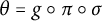 $\theta =g\circ \pi \circ \sigma $
, where
 $g\in G$
,
 $\pi =\pi _{\theta }$
is a Dynkin diagram automorphism, and
 $\sigma $
is a field automorphism (in the special characteristic case,
 $\pi $
is a Coxeter diagram automorphism). Note that the “diagonal automorphisms” are already built into G. By the Bruhat decomposition, each element
 $g\in G$
can be written as
 $g=uwb$
with
 $u\in U^+$
,
 $w\in W$
, and
 $b\in B$
, and so each automorphism of
 $\Delta $
can be written as
 $\theta =uwb\circ \pi \circ \sigma $
. If
 $\sigma $
is trivial, we say that
 $\theta $
is linear.
By a root elation, we shall mean an automorphism
 $\theta $
conjugate to
 $x_{\alpha }(a)$
for some
 $\alpha \in \Phi $
and
 $a\in \mathbb {F}^{\times }$
, and we call
 $\theta $
a long (respectively short) root elation if
 $\alpha $
is a long (respectively short) root. By a homology, we shall mean an automorphism
 $\theta $
conjugate to a nontrivial element
 $h_{\lambda }(c)$
with
 $\lambda \in P$
and
 $c\in \mathbb {F}^{\times }$
.
We often regard
 $\Delta $
as a simplicial complex in the standard way (cf. [Reference Abramenko and Brown1, Chapter 4]). Let us briefly describe this conversion in a group theoretic way in the split context. For subsets
 $J\subseteq S$
, let
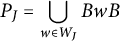 $$ \begin{align*}P_{J}=\bigcup_{w\in W_{J}}BwB \end{align*} $$
be the standard parabolic subgroup of G of type J. For each nonempty
 $J\subseteq S$
, the set of “type J-simplices” of the building is the set of cosets
 $G/P_{S\backslash J}$
, and the simplicial complex structure is given by reverse containment of cosets. For example, in the simplicial complex language, the chamber B “contains” the simplices
 $P_{S\backslash J}$
for all nonempty
 $J\subseteq S$
, whereas on the level of cosets, it is, in fact, the parabolic subgroups
 $P_{S\backslash J}$
that contain the Borel subgroup B.
If
 $J=\{s\}$
is a singleton, we often write
 $$ \begin{align} W_s=W_{S\backslash J}\quad\text{and}\quad P_s=W_{S\backslash J} \end{align} $$
for the standard parabolic subgroups of W and G of type
 $S\backslash J$
. Moreover, if
 $s=s_i$
, we will often write
 $W_{s_i}=W_i$
and
 $P_{s_i}=P_i$
.
Let
 $\tau (x)\subseteq S$
denote the type of the simplex x of
 $\Delta $
. Thus, vertices are simplices x with
 $\tau (x)=\{s\}$
for some
 $s\in S$
, and chambers are the simplices x with
 $\tau (x)=S$
. A panel is a codimension
 $1$
simplex; that is,
 $\tau (x)=S\backslash \{s\}$
, for some
 $s\in S$
.
Note that we use the same symbol
 $\Delta $
for the building regarded as either a set of chambers with a Weyl distance function (as in Definition 2.4) or as a simplicial complex (as outlined above). No confusion will arise from this convention.
2.3 Opposition diagrams and admissible diagrams
Chambers
 $c,d\in \Delta $
are opposite one another if and only if
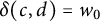 $\delta (c,d)=w_0$
. If
 $x,y$
are simplices, with types
 $J,K$
, respectively, then x and y are opposite one another if and only if
 $K=\pi _0(J)$
and there exist opposite chambers
 $c,d$
with
 $x\subseteq c$
and
 $y\subseteq d$
. That is, simplices are opposite one another if they have opposite types, and are contained in opposite chambers. In terms of double cosets, chambers
 $c=gB$
and
 $d=hB$
are opposite if and only if
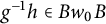 $g^{-1}h\in Bw_0B$
, and simplices
 $x=gP_{S\backslash J}$
and
 $y=hP_{S\backslash K}$
are opposite if and only if
 $K=\pi _0(J)$
and
 $g^{-1}h\in P_{S\backslash J}w_0P_{S\backslash K}$
.
Let
 $\theta $
be an automorphism of
 $\Delta $
. Recall, from the introduction, that
 $\operatorname {{\mathrm {Opp}}}(\theta )$
denotes the set of all simplices x such that
 $x^{\theta }$
is opposite x. The type
 $\operatorname {{\mathrm {Typ}}}(\theta )$
of
 $\theta $
is the union of all subsets
 $J\subseteq S$
such that there exists a type J simplex mapped to an opposite simplex by
 $\theta $
. The opposition diagram of
 $\theta $
is the triple
 $(\Gamma ,\operatorname {{\mathrm {Typ}}}(\theta ),\pi _{\theta })$
.
Less formally, the opposition diagram of
 $\theta $
is depicted by drawing
 $\Gamma $
and encircling the nodes of
 $\operatorname {{\mathrm {Typ}}}(\theta )$
, where we encircle nodes in minimal subsets invariant under
 $\pi _0\circ \pi _{\theta }$
. We draw the diagram “bent” (in the standard way) if
 $\pi _0\circ \pi _{\theta }\neq \mathrm {id}$
. For example, consider the diagrams

Diagram
 $\mathsf {X}$
represents a collineation
 $\theta $
of an
 $\mathsf {E}_6$
building with
 $\operatorname {{\mathrm {Typ}}}(\theta )=\{1,2,6\}$
, and diagram
 $\mathsf {Y}$
represents a duality of an
 $\mathsf {E}_6$
building with
 $\operatorname {{\mathrm {Typ}}}(\theta )=\{1,6\}$
.
An automorphism
 $\theta $
is domestic if
 $\operatorname {{\mathrm {Opp}}}(\theta )$
contains no chamber (that is,
 $\theta $
maps no chamber to an opposite chamber). More generally, if
 $J\subseteq S$
, then
 $\theta $
is J-domestic if no type J simplex is mapped onto an opposite simplex by
 $\theta $
. To avoid trivialities, the definition of J-domesticity is restricted to subsets J with
 $\pi _0(J)=\pi _{\theta }(J)$
(for if J does not satisfy this, then
 $\theta $
is J-domestic for trivial reasons).
An automorphism
 $\theta $
is called capped if the following closure property holds: If there exist type
 $J_1$
and
 $J_2$
simplices in
 $\operatorname {{\mathrm {Opp}}}(\theta )$
, then there exists a type
 $J_1\cup J_2$
simplex in
 $\operatorname {{\mathrm {Opp}}}(\theta )$
. Equivalently,
 $\theta $
is capped if and only if there exists a type
 $\operatorname {{\mathrm {Typ}}}(\theta )$
simplex in
 $\operatorname {{\mathrm {Opp}}}(\theta )$
. By [Reference Parkinson and Van Maldeghem15, Theorem 1], every automorphism of a “large” spherical building of rank at least
 $3$
is capped, where a building is called large if it contains no Fano plane residues (for split buildings, this simply means
 $|\mathbb {F}|>2$
).
In [Reference Parkinson and Van Maldeghem15, Reference Parkinson and Van Maldeghem16], we showed that the opposition diagrams of automorphisms of spherical buildings satisfy various restrictive properties, and we used these properties to determine a list of all possible opposition diagrams. We call the diagrams
 $(\Gamma ,J,\pi )$
in this list admissible Dynkin diagrams (more precisely, in [Reference Parkinson and Van Maldeghem15, Reference Parkinson and Van Maldeghem16], we considered Coxeter diagrams rather than Dynkin diagrams; however, the arguments are nearly identical).
The complete list of admissible Dynkin diagrams of exceptional type is given in Figure 1 (taken from [Reference Parkinson and Van Maldeghem15]). Each admissible diagram
 $(\Gamma ,J,\pi )$
of exceptional type is denoted by a symbol
 $$ \begin{align*}{^t}\mathsf{X}_{n;i}\quad\text{or}\quad {^t}\mathsf{X}_{n;i}^{k}, \end{align*} $$
where:
-
(1)
$\mathsf {X}\in \{\mathsf {E},\mathsf {F},\mathsf {G}\}$
is the type of
$\Gamma $
, and n is the rank; -
(2)
$t\in \{1,2\}$
is the order of the graph automorphism
$\pi _0\circ \pi $
(the “twisting”); -
(3) i is the number of distinguished orbits contained in J; and
-
(4) k is an additional index occurring only for
$\mathsf {F}_4$
and
$\mathsf {G}_2$
in the case that a single node is encircled, in which case k is the type of this node.



In the case
 $t=1$
(that is, when
 $\pi _0\circ \pi =\mathrm {id}$
), we usually omit the t from the notation, writing simply
 ${^1}\mathsf {X}_{n;i}=\mathsf {X}_{n;i}$
. For example, the diagrams
 $\mathsf {X}$
and
 $\mathsf {Y}$
given above are
 $\mathsf {X}={^2}\mathsf {E}_{6;2}$
and
 $\mathsf {Y}=\mathsf {E}_{6;2}$
. Similar notation is introduced in [Reference Parkinson and Van Maldeghem17] for the classical types (except with a different meaning for the index k).
In special characteristic, one often ignores the arrows on Dynkin diagrams, thus giving the additional admissible (Coxeter) diagrams in Figure 2.
Additional admissible diagrams for special characteristic.

Summarizing the above discussion, we have the following from [Reference Parkinson and Van Maldeghem15, Reference Parkinson and Van Maldeghem16].
Theorem 2.5 If
 $\theta $
is an automorphism of a spherical building of exceptional type, then the opposition diagram of
 $\theta $
is listed in Figure 1 or 2.
A striking feature of Theorem 2.5 is that there are very few possible opposition diagrams. We note that the analysis in [Reference Parkinson and Van Maldeghem15, Reference Parkinson and Van Maldeghem16] does not prove the converse to Theorem 2.5. That is, a priori, there may be redundancies in the list of admissible diagrams, in the sense that some admissible diagrams may not actually be the opposition diagram of any automorphism of any spherical building. It is a consequence of the work of this paper, combined with [Reference Parkinson and Van Maldeghem17], that no such redundancies exist—more precisely, Corollary 10 holds.
We call an admissible diagram empty if no nodes are encircled, and full if all nodes are encircled. We call an admissible diagram
 $(\Gamma ,J,\pi )$
type preserving if
 $\pi =\mathrm {id}$
. By inspection of the list in Figure 1, we note that for each Dynkin diagram
 $\Gamma $
, the type preserving diagram
 $(\Gamma ,\wp ,\mathrm {id})$
(with
 $\wp $
the polar type) is admissible. This diagram is called the polar diagram.
The polar–copolar diagram is the type preserving admissible diagram with
 $J=\wp \cup \wp ^*$
, where
 $\wp ^*$
is the polar type of the type
 $S\backslash \wp $
residue (we call
 $\wp ^*$
the copolar type; again, by inspection of Figure 1, the triple
 $(\Gamma ,\wp \cup \wp ^*,\mathrm {id})$
is always an admissible diagram). See Appendix A for the list of polar and copolar types. Alternatively, the polar–copolar diagrams of exceptional type are characterized as the type preserving diagrams in which exactly two orbits of nodes are encircled. Specifically, the polar diagrams of exceptional type are
 ${^2}\mathsf {E}_{6;1}$
,
 $\mathsf {E}_{7;1}$
,
 $\mathsf {E}_{8;1}$
,
 $\mathsf {F}_{4;1}^1$
, and
 $\mathsf {G}_{2;1}^2$
, and the polar–copolar diagrams are
 ${^2}\mathsf {E}_{6;2}$
,
 $\mathsf {E}_{7;2}$
,
 $\mathsf {E}_{8;2}$
,
 $\mathsf {F}_{4;2}$
, and
 $\mathsf {G}_{2;2}$
.
Every duality of a thick
 $\mathsf {G}_2$
(respectively
 $\mathsf {F}_4$
) building has opposition diagram
 ${^2}\mathsf {G}_{2;1}$
(respectively
 ${^2}\mathsf {F}_{4;2}$
), and no such dualities are domestic (see [Reference Parkinson, Temmermans and Van Maldeghem14, Theorem 2.7] and [Reference Parkinson and Van Maldeghem15, Lemma 4.1]). We note that dualities of split
 $\mathsf {F}_4$
and
 $\mathsf {G}_2$
buildings only exist for perfect fields of special characteristic.
2.4 Basic techniques
It is generally rather difficult to prove that a given automorphism is domestic, and more challenging to compute its opposition diagram. In this section, we describe some of the techniques that we will use in this paper.
The displacement of an automorphism
 $\theta $
is
 $$ \begin{align*}\operatorname{{\mathrm{disp}}}(\theta)=\max\{\ell(\delta(c,c^{\theta}))\mid c\in\Delta\}. \end{align*} $$
Thus,
 $\theta $
is domestic if and only if
 $\operatorname {{\mathrm {disp}}}(\theta )<\ell (w_0)$
. Moreover, by [Reference Parkinson and Van Maldeghem16, Corollary 2.29], we have, with
 $J=\operatorname {{\mathrm {Typ}}}(\theta )$
,
 $$ \begin{align*}\operatorname{{\mathrm{disp}}}(\theta)=\begin{cases} \ell(w_{S\backslash J}w_0)&\text{if}\ \theta\ \text{is capped}\\ \ell(w_{S\backslash J}w_0)-1&\text{if}\ \theta\ \text{is uncapped.} \end{cases} \end{align*} $$
Uncapped automorphisms will not play a significant role here, so assume that
 $\theta $
is capped. By the above comments, and the classification of admissible diagrams, the list of possible displacements of
 $\theta $
is very restricted. For example, for a capped automorphism of an
 $\mathsf {E}_7$
building, the displacements for the nonfull nonempty opposition diagrams are:
 $$ \begin{align*} 33\text{ for}\ \mathsf{E}_{7;1},\quad 50\text{ for}\ \mathsf{E}_{7;2},\quad 51\text{ for}\ \mathsf{E}_{7;3},\quad 60\text{ for}\ \mathsf{E}_{7;4}. \end{align*} $$
Thus, for example, to show that a capped automorphism
 $\theta $
of an
 $\mathsf {E}_7$
building:
-
(1) is not domestic, it is sufficient to show that
$\operatorname {{\mathrm {disp}}}(\theta )>60$
; -
(2) has opposition diagram
$\mathsf {E}_{7;3}$
, it is sufficient to show that
$\operatorname {{\mathrm {disp}}}(\theta )<60$
and that there is a type
$\{1,6,7\}$
simplex mapped to an opposite (in fact, from the classification of diagrams, it would be sufficient to show that there is a type
$7$
vertex mapped to an opposite).





Such arguments will be used on multiple occasions throughout the paper.
The following lemma is useful to compute displacement, and Corollary 2.7 is useful to prove J-domesticity.
Lemma 2.6 Let
 $\theta $
be an automorphism of a thick spherical building
 $\Delta $
, and let
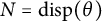 $N=\operatorname {{\mathrm {disp}}}(\theta )$
. Let c be any chamber. Suppose that either:
-
(1) each panel of
$\Delta $
has at least four chambers, or -
(2)
$\theta $
is an involution, or -
(3)
$\theta $
induces opposition and
$N=\ell (w_0)$
.


Then,
 $\theta $
is necessarily capped, and there exists a chamber d with
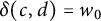 $\delta (c,d)=w_0$
and
 $\ell (\delta (d,d^{\theta }))=N$
. In particular,
 $$ \begin{align*}\operatorname{{\mathrm{disp}}}(\theta)=\max\{\ell(\delta(d,d^{\theta}))\mid d\in \Delta\text{ with}\ \delta(c,d)=w_0\}. \end{align*} $$
Proof To see that
 $\theta $
is capped: If each panel has at least four chambers, then
 $\theta $
is capped by [Reference Parkinson and Van Maldeghem15, Theorem 1], if
 $\theta $
is an involution, then
 $\theta $
is capped by [Reference Parkinson and Van Maldeghem16, Corollary 2.22], and if
 $\operatorname {{\mathrm {disp}}}(\theta )=\ell (w_0)$
, then
 $\theta $
maps a chamber to an opposite, and hence is capped. The rest of the lemma is contained in [Reference Parkinson and Van Maldeghem16, Lemma 4.1].▪
Corollary 2.7 Let
 $\theta $
be an automorphism of a thick spherical building
 $\Delta $
, and suppose that the hypothesis of Lemma 2.6 is satisfied. Let c be any chamber. For each subset
 $J\subseteq S$
, the automorphism
 $\theta $
is J-domestic if and only if it is J-domestic when restricted to the sphere of chambers opposite c. That is, for every chamber d with
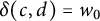 $\delta (c,d)=w_0$
, the type J-simplex of d is not mapped onto an opposite simplex.
Proof Clearly, if
 $\theta $
is J-domestic, then it is also J-domestic when restricted to the set of chambers opposite c. Conversely, suppose that
 $\theta $
is not J-domestic. Let
 $J'=\operatorname {{\mathrm {Typ}}}(\theta )$
, and so
 $J\subseteq J'$
. By Lemma 2.6,
 $\theta $
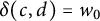
is capped, and there is a chamber d with
 $\delta (c,d)=w_0$
such that
 $\ell (\delta (d,d^{\theta }))=\operatorname {{\mathrm {disp}}}(\theta )$
. Because
 $\theta $
is capped, by [Reference Parkinson and Van Maldeghem15, Theorem 2.6], we have
 $\delta (d,d^{\theta })=w_{S\backslash J'}w_0$
. In particular, the type
 $J'$
-simplex of d is mapped to an opposite simplex, and hence the type
 $J\subseteq J'$
simplex of d is mapped to an opposite simplex (note that necessarily
 $\pi _0(J)=\pi _{\theta }(J)$
, because there exists a type J-simplex mapped to an opposite simplex by hypothesis). Hence,
 $\theta $
is not J-domestic when restricted to the set of chambers opposite c.▪
The following proposition gives a useful technique for proving domesticity. We refer to this technique as the “standard technique.”
Proposition 2.8 Let
 $\Delta =\Delta _{\Phi }(\mathbb {F})$
be split, and let
 $\theta \in G=G_{\Phi }(\mathbb {F})$
. Suppose that the hypothesis of Lemma 2.6 is satisfied for the automorphism
 $\theta $
. If there is
 $w_1\in W$
with
 $$ \begin{align*}w_1^{-1}w_0^{-1}u^{-1}\theta uw_0w_1\in B\quad\text{for all}\ u\in U^+, \end{align*} $$
then
 $ \operatorname {{\mathrm {disp}}}(\theta )\leq 2\ell (w_1)-1$
. Thus, in particular, if
 $\ell (w_1)\leq \ell (w_0)/2$
, then
 $\theta $
is domestic.
Proof Each chamber
 $gB$
of the building
 $G/B$
can be written uniquely as
 $uwB$
for some
 $w\in W$
and some
 $u\in \langle U_{\alpha }\mid \alpha \in \Phi (w)\rangle $
. Then,
 $\delta (gB,\theta gB)$
is the unique element
 $v\in W$
such that
 $w^{-1}u^{-1}\theta uw\in BvB$
. If the hypothesis of Lemma 2.6 is satisfied, then the displacement of
 $\theta $
is achieved for some chamber
 $gB$
opposite the base chamber B. These chambers are of the form
 $uw_0B$
with
 $u\in U^+$
. By the hypothesis, we have
 $$ \begin{align*}w_0^{-1}u^{-1}\theta uw_0\in w_1Bw_1^{-1}\subseteq Bw_1B\cdot Bw_1^{-1}B. \end{align*} $$
In particular, if
 $w=\delta (uw_0B,\theta uw_0B)$
, then
 $BwB\subseteq Bw_1B\cdot Bw_1^{-1}B$
. Thus,
 $$ \begin{align} \operatorname{{\mathrm{disp}}}(\theta)\leq\max\{\ell(w)\mid BwB\subseteq Bw_1B\cdot Bw_1^{-1}B\}. \end{align} $$
Writing
 $w_1=w_2s$
with
 $\ell (w_2s)=\ell (w_2)+1$
, by (2.3), we have
 $$ \begin{align*}Bw_1B\cdot Bw_1^{-1}B=(Bw_2sB\cdot Bw_2^{-1}B)\cup (Bw_2B\cdot Bw_2^{-1}B),\end{align*} $$
and it follows from (2.3) that
 $ \operatorname {{\mathrm {disp}}}(\theta )\leq 2\ell (w_1)-1$
.▪
In the case that
 $\theta \in U^+$
, the following lemma is helpful in finding an element
 $w_1\in W$
as in Proposition 2.8. If
 $A\subseteq \Phi $
, let
 $ A_{\geq }=\{\beta \in \Phi \mid \beta \geq \alpha \text { for some}\ \alpha \in A\}, $
where
 $\alpha \leq \beta $
if and only if
 $\beta -\alpha $
is a nonnegative linear combination of positive roots. Let
 $\pi _0$
be the automorphism of
 $\Phi $
given by
 $\pi _0(\alpha )=-w_0\alpha $
(thus,
 $\pi _0$
is the automorphism induced by the opposition diagram automorphism).
Lemma 2.9 If
 $\theta \in \langle U_{\alpha }\mid \alpha \in A\rangle $
for some
 $A\subseteq \Phi ^+$
, then
 $ u^{-1}\theta u\in \langle U_{\alpha }\mid \alpha \in A_{\geq }\rangle , $
for all
 $u\in U^+$
. Moreover, if
 $w_1\in W$
is such that
 $\pi _0(A_{\geq })\subseteq \Phi (w_1)$
, then
 $w_1^{-1}w_0^{-1}u^{-1}\theta u w_0w_1\in B$
for all
 $u\in U^+$
.
Proof Let
 $F=\langle U_{\alpha }\mid \alpha \in A_{\geq }\rangle $
. If
 $\beta \in \Phi ^+$
and
 $\alpha \in A_{\geq }$
, then by commutator relations, we have, for all
 $a\in \mathbb {F}$
,
 $ x_{\beta }(a)^{-1}U_{\alpha }x_{\beta }(a)\subseteq U_{\alpha }U_{\alpha +\beta }U_{2\alpha +\beta }\cdots \subseteq F$
(with the convention that
 $U_{\gamma }=\{1\}$
if
 $\gamma \notin \Phi $
). It follows that
 $x_{\beta }(a)^{-1}Fx_{\beta }(a)\subseteq F$
. Thus, by induction,
 $u^{-1}Fu\subseteq F$
for all
 $u\in U$
, and because
 $\theta \in F$
, we have
 $u^{-1}\theta u\in F$
as required. Thus, if
 $w_1\in W$
is such that
 $\pi _0(A_{\geq })\subseteq \Phi (w_1)$
, then
 $$ \begin{align*}w_0^{-1}u^{-1}\theta u w_0\in \langle U_{-\alpha}\mid \alpha\in \pi_0(A_{\geq})\rangle =w_1\langle U_{-w_1^{-1}\alpha}\mid \alpha\in \pi_0(A_{\geq})\rangle w_1^{-1}, \end{align*} $$
which is contained in
 $w_1Bw_1^{-1}$
, and hence the result.▪
2.5 Parapolar spaces and Lie incidence geometries
At certain points of this paper (in particular, in Section 6), we will work with Lie incidence geometries
 $\mathsf {X}_{n,J}(\mathbb {F})$
, for example, the long root geometries
 $\mathsf {E}_{6,2}(\mathbb {F})$
,
 $\mathsf {E}_{7,1}(\mathbb {F})$
,
 $\mathsf {E}_{8,8}(\mathbb {F})$
, and
 $\mathsf {F}_{4,1}(\mathbb {F})$
, and the geometries
 $\mathsf {E}_{6,1}(\mathbb {F})$
,
 $\mathsf {E}_{7,7}(\mathbb {F})$
, and
 $\mathsf {F}_{4,4}(\mathbb {F})$
. We note the similarity of notation with that used for opposition diagrams; however, no confusion should arise.
In general, the Lie incidence geometry
 $\mathsf {X}_{n,J}(\mathbb {F})$
, with
 $J\subseteq S$
, is defined from the building
 $\Delta =\Delta _\Phi (\mathbb {F})$
, with
 $\Phi $
the root system of type
 $\mathsf {X}_n$
, as the point-line geometry with point set, the set of simplices (or flags) of type J of
 $\Delta $
, and a typical line is the set of flags of type J incident with a flag of type
 $S\backslash \{j\}$
for some
 $j\in J$
. If
 $J=\wp $
, then we call the geometry
 $\mathsf {X}_{n,J}(\mathbb {F})$
a long root geometry.
The geometries listed in the first paragraph of this subsection are all examples of parapolar spaces (see [Reference Shult21, Chapter 13] for the basic terminology and definition). In particular, these point-line geometries
 $\mathscr {G}=(\mathcal {P},\mathcal {L})$
contain symplecta (or symps for short), being convex subsets that are nondegenerate polar spaces of rank at least
 $2$
. If all symplecta have the same rank
 $r\geq 2$
, then
 $\mathscr {G}$
is said to have symplectic rank r. Recall that in any incidence geometry,
 $x^{\perp }$
denotes the set of all points collinear to the point x. In addition, each symp
 $\xi $
is, by convexity, determined by any pair
 $\{x,y\}$
of noncollinear points, and we denote
 $\xi =\xi (x,y)$
. If
 $\mathsf {X}_n=\mathsf {E}_6,\mathsf {E}_7,\mathsf {E}_8,\mathsf {F}_4$
, then
 $\mathsf {X}_{n,\wp }(\mathbb {F})$
has symplectic rank
 $4,5,7,3$
, respectively. Moreover, the symps precisely correspond to the residues of vertices of type
 $\wp ^*$
.
In the parapolar spaces
 $\mathsf {E}_{6,2}(\mathbb {F})$
,
 $\mathsf {E}_{7,1}(\mathbb {F})$
,
 $\mathsf {E}_{8,8}(\mathbb {F})$
,
 $\mathsf {F}_{4,1}(\mathbb {F})$
, and
 $\mathsf {F}_{4,4}(\mathbb {F})$
, there are precisely five possible “distances” between two points
 $x,y$
. Either (1)
 $x=y$
, (2) x and y are collinear, (3)
 $\{x,y\}$
lies in a symplecton, (4)
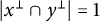 $|x^{\perp }\cap y^{\perp }|=1$
, or (5)
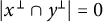 $|x^{\perp }\cap y^{\perp }|=0$
. In case (3), we say that
 $x,y$
are symplectic (or at symplectic distance), and we denote by
 $x^{\perp \!\!\!\perp }$
the set of points at symplectic distance from x. In case (4), we say that
 $x,y$
are special (or a special pair, or at special distance), and we denote by
 $x^{\Join }$
the set of points at special distance from x. Finally, in case (5), the points
 $x,y$
are opposite each other (in the building theoretic sense).
The parapolar spaces
 $\mathsf {F}_{4,1}(\mathbb {F})$
and
 $\mathsf {F}_{4,4}(\mathbb {F})$
are also called metasymplectic spaces. In the parapolar spaces
 $\mathsf {E}_{6,1}(\mathbb {F})$
and
 $\mathsf {E}_{7,7}(\mathbb {F})$
, there are no special pairs, and so in these spaces, there are only four possible distances between two points (these spaces are called strong parapolar spaces).
An imaginary line of a long root geometry
 $\mathscr {G}$
is a set of the form
 $x^T\cup \{y\}$
, where
 $x,y$
are opposite points, and T is the full collineation group of central elations with center y. Note that if
 $\mathscr {G}$
is a polar space of rank at least
 $3$
, or if
 $\mathscr {G}$
is a Moufang quadrangle, then
 $x^T\cup \{y\}=(\{x,y\}^{\perp })^{\perp }$
for opposite points
 $x,y$
.
Let us briefly describe the long root geometry parapolar spaces in more algebraic terms. Let
 $\mathsf {X}_n=\mathsf {E}_n$
(
 $n=6,7,8$
) or
 $\mathsf {F}_4$
, and let
 $p\in S$
be the polar node. Recall the notation (2.5). Let
 $M_p$
denote the set of minimal length coset representatives of cosets in
 $W/W_p$
, and let
 $R_p$
denote the set of minimal length representatives for the double cosets in
 $W_p\backslash W/W_p$
. The points of the long root geometry
 $\mathsf {X}_{n,p}(\mathbb {F})$
are the cosets in
 $G/P_p$
. We have
 $ G=\bigsqcup _{w\in R_p}P_pwP_p, $
and the Weyl-distance
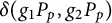 $\delta (g_1P_p,g_2P_p)$
between points
 $g_1P_p$
and
 $g_2P_p$
is defined to be the unique element
 $\delta (g_1P_p,g_2P_p)=w\in R_p$
with
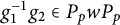 $g_1^{-1}g_2\in P_pwP_p$
.
In each case,
 $R_p$
contains precisely five elements
 $e,s_p,w_1,w_2,s_{\varphi }$
, arranged in increasing length, corresponding to the five possible distances between points. Explicitly, the points
 $x=g_1P_p$
and
 $y=g_2P_p$
are collinear (respectively symplectic, at special distance, opposite) if
 $\delta (x,y)=s_p$
(respectively
 $w_1$
,
 $w_2$
,
 $s_{\varphi }$
). Similar remarks hold for the metasymplectic space
 $\mathsf {F}_{4,4}(\mathbb {F})$
, and also the strong parapolar spaces
 $\mathsf {E}_{6,1}(\mathbb {F})$
and
 $\mathsf {E}_{7,7}(\mathbb {F})$
(where only four distances are possible, and hence
 $w_2$
is omitted).
3 Root elations and the polar type
In this section, we prove Theorem 1 for exceptional types (see Theorems 3.1 and 3.4). In fact, we focus on types
 $\mathsf {E}_6,\mathsf {E}_7,\mathsf {E}_8$
, and
 $\mathsf {F}_4$
, with the case of
 $\mathsf {G}_2$
following from the classification in Theorem 9 (see Section 7.3). We also provide a geometric characterization of root elations for buildings of types
 $\mathsf {E}_6$
and
 $\mathsf {E}_7$
in Theorem 3.6, and we discuss short root elations in the nonsimply laced case in Theorem 3.10. The proofs of Corollaries 2 and 3 are given in Sections 3.1 and 3.3, respectively (see also Corollary 3.11).
3.1 Long root elations
To prove Theorem 1, we must first show that long root elations have polar opposition diagram, and conversely that every automorphism with polar opposition diagram is necessarily a long root elation. We prove the first statement in Theorem 3.1 in a more general context of Moufang spherical buildings, and the second statement is proved in Theorem 3.4.
Let
 $\Delta $
be an irreducible Moufang spherical building. Recall (for example, from [Reference Timmesfeld27]) that if
 $\Delta $
is not a generalized octagon, then one can associate a crystallographic (not necessarily reduced) root system
 $\Phi $
to
 $\Delta $
in such a way that the root subgroup
 $U_{\varphi }$
, with
 $\varphi $
the highest root of
 $\Phi $
, is contained in the center of the positive root subgroup
 $U^+=\langle U_{\alpha }\mid \alpha \in \Phi ^+\rangle $
. In the case that
 $\Phi $
has only one root length, we call all roots long. Let
 $\wp \subseteq S$
denote the polar type of the Dynkin diagram of
 $\Phi $
. If
 $\Delta $
is a generalized octagon, then by [Reference Tits29], one may associate a noncrystallographic (and nonreduced) root system
 $\Phi $
, and again, there is a “highest root”
 $\varphi $
such that
 $U_{\varphi }$
is contained in the center of
 $U^+$
(the root
 $\varphi $
is
 $\alpha _4^{\prime }$
in [Reference Tits29], and the polar type corresponds to “points” of the octagon). In all cases, let W be the Weyl group of
 $\Phi $
(so W is a dihedral group of order
 $16$
in the octagon case).
Theorem 3.1 Let
 $\Delta $
be an irreducible Moufang spherical building with associated root system
 $\Phi $
and Weyl group W as above. Let
 $\alpha \in \Phi $
be a long root, and let
 $\theta \in U_{\alpha }\backslash \{1\}$
. Then, the collineation
 $\theta $
of
 $\Delta =G/B$
has polar opposition diagram. Moreover,
 $$ \begin{align} \{\delta(c,c^{\theta})\mid c\in \Delta\}=\{1\}\cup\{s_{\alpha}\mid \alpha\in W\varphi\}. \end{align} $$
Proof Because
 $\alpha $
is a long root, it is in the W-orbit of the highest root, and it follows from standard root group datum (RGD) properties (see [Reference Abramenko and Brown1, Section 7.8]) that
 $\theta $
is conjugate to an element of
 $U_{\varphi }\backslash \{1\}$
. Thus, after conjugation, we may assume that
 $\theta $
is central in
 $U^+$
. A chamber
 $gB$
is opposite its image
 $\theta gB$
if and only if
 $\delta (gB,\theta gB)=w_0$
, if and only if
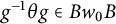 $g^{-1}\theta g\in Bw_0B$
. By the Bruhat decomposition, each chamber
 $gB$
can be written as
 $ gB=uwB$
for some
 $u\in U^+$
and
 $w\in W$
. Because
 $\theta $
is central in
 $U^+$
, we have
 $ w^{-1}u^{-1}\theta uw=w^{-1}\theta w\in U_{w^{-1}\varphi } $
. Thus, if
 $w^{-1}\varphi \in \Phi ^+$
, we have
 $\delta (gB,\theta gB)=1$
, and if
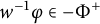 $w^{-1}\varphi \in -\Phi ^+$
, then
 $w^{-1}\theta w\in U_{w^{-1}\varphi }\subseteq Bs_{w^{-1}\varphi }B$
, and so
 $\delta (gB,\theta gB)=s_{w^{-1}\varphi }$
. Equation (3.1) follows.
Because
 $\theta $
is a nontrivial collineation, there is some simplex mapped onto an opposite simplex. Let
 $J\subseteq S$
be the type of such a simplex x, and write
 $J^{\prime }=S\backslash J$
. Thus, for each chamber
 $c\in \Delta $
containing x, we have
 $\delta (c,c^{\theta })\in W_{J^{\prime }}w_0W_{J^{\prime }}$
. Because J, and hence also
 $J^{\prime }$
, are stable under opposition, we have
 $W_{J^{\prime }}w_0W_{J^{\prime }}=w_0W_{J^{\prime }}$
. It follows from (3.1) that there is a root
 $\alpha \in W\varphi $
with
 $s_{\alpha }=w_0w$
for some
 $w\in W_{J^{\prime }}$
. Because
 $W_{J^{\prime }}$
is a proper parabolic subgroup of W, each
 $w\in W_{J^{\prime }}$
maps the highest root
 $\varphi $
to a positive root, and because
 $w_0$
maps all positive roots to negative roots, we have
 $s_{\alpha }\varphi \in -\Phi ^+$
. Because
 $\varphi $
is the highest root of
 $\Phi $
, this forces
 $\alpha =\pm \varphi $
, and so
 $w_0^{-1}s_{\varphi }\in W_{J^{\prime }}$
. For all
 $t\in S$
, we have
 $$ \begin{align*}w_0^{-1}s_{\varphi}(\alpha_t)=-\alpha_{\pi_0(t)}+\langle\alpha_t,\varphi^{\vee}\rangle\varphi \end{align*} $$
(where
 $\pi _0(t)=w_0tw_0^{-1}$
), and because
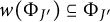 $w(\Phi _{J^{\prime }})\subseteq \Phi _{J^{\prime }}$
for all
 $w\in W_{J^{\prime }}$
, we deduce that
 $\langle \alpha _t,\varphi ^{\vee }\rangle =0$
for all
 $t\in {J^{\prime }}=S\backslash J$
. It follows that
 $J=\wp $
.▪
We now prove Corollary 2, which is restated below for convenience.
Corollary 3.2 Every irreducible Moufang spherical building distinct from a projective plane admits a nontrivial domestic collineation.
Proof This follows immediately from Theorem 3.1 and the fact that
 $\wp $
is a strict subset of S in all cases except for
 $\Phi =\mathsf {A}_2$
(which is the case of projective planes).▪
Remark 3.3 Theorem 3.1 implies that every Ree–Tits octagon admits nontrivial line-domestic collineations. We note that it is erroneously stated in [Reference Ihringer, Sin and Xiang11] that these octagons do not admit line-domestic collineations. The error appears to be as follows. If a thick generalized octagon admits a line-domestic collineation
 $\theta $
, then by [Reference Parkinson, Temmermans and Van Maldeghem14, Theorem 2.8 and Proposition 4.1], the fixed element structure of
 $\theta $
is either a large full suboctagon, a distance
 $4$
-ovoid, or a ball of radius
 $4$
in the incidence graph centered at a point. For finite Ree–Tits octagons, we proved in [Reference Parkinson, Temmermans and Van Maldeghem14, Proposition 4.4] that large full suboctagons do not exist, and in [Reference Ihringer, Sin and Xiang11], it is shown that distance
 $4$
-ovoids do not exist. Thus, any line-domestic collineation of a finite Ree–Tits octagon necessarily fixes a ball of radius
 $4$
centered at a point (and is thus a central collineation, the example given by Theorem 3.1). It follows from [Reference Parkinson, Temmermans and Van Maldeghem14, Proposition 4.5] that no collineation of a finite Ree–Tits octagon fixes a ball of radius
 $4$
centered at a line, and we believe that this may be the source of the misunderstanding in [Reference Ihringer, Sin and Xiang11] (with
 $s=t^2$
misread as
 $s^2=t$
in [Reference Parkinson, Temmermans and Van Maldeghem14, Proposition
4.5]).
We now prove the converse to Theorem 3.1 for split buildings of types
 $\mathsf {E}_n$
and
 $\mathsf {F}_4$
. Let
 $\Phi $
be a root system of type
 $\mathsf {E}_n$
for
 $n=6,7,8$
, or of type
 $\mathsf {F}_4$
. Let
 $\varphi $
be the highest root. Let
 $i_0$
be the polar node. Let
 $\Phi _1$
be the polar subsystem, generated by the simple roots
 $\{\alpha _i\mid i\neq i_0\}$
, and let
 $W_1$
be the parabolic subgroup generated by
 $\{s_i\mid i\neq i_0\}$
. Let
 $w_0$
be the longest element, and let
 $w_1$
be the longest element of
 $W_1$
. Let
 $j_0$
be the unique node joined to the polar node in the Dynkin diagram. Write
 $\pi =\alpha _{i_0}$
and
 $\pi ^{\prime }=\alpha _{j_0}$
. Explicitly,
 $(\pi ,\pi ^{\prime })=(\alpha _2,\alpha _4)$
,
 $(\alpha _1,\alpha _3)$
,
 $(\alpha _8,\alpha _7)$
, and
 $(\alpha _1,\alpha _2)$
for types
 $\mathsf {E}_6$
,
 $\mathsf {E}_7$
,
 $\mathsf {E}_8$
, and
 $\mathsf {F}_4$
, respectively. Let
 $\omega =\omega _{i_0}$
be the fundamental coweight corresponding to the polar node (thus
 $\langle \omega ,\alpha _{i}\rangle = \delta _{i,i_0}$
). We note the following facts:
-
(1)
$\omega =\varphi ^{\vee }$
(because
$\langle \varphi ^{\vee },\alpha _{i}\rangle =\delta _{i,i_0}$
). -
(2)
$\varphi $
is the unique root whose coefficient of
$\pi $
is
$2$
(because
$2=\langle \varphi ,\varphi ^{\vee }\rangle =\langle \varphi ,\omega \rangle $
). -
(3)
$\varphi -\alpha _i\in \Phi $
if and only if
$i=i_0$
(by (2)). -
(4) The elements
$\varphi -\pi $
and
$\varphi -\pi -\pi ^{\prime }$
are roots, but
$\varphi -\pi ^{\prime }$
is not a root (by (2)). -
(5)
$s_{\varphi }=w_1w_0$
(as both have inversion set
$\Phi ^+\backslash \Phi _1=\{\alpha \in \Phi ^+\mid \langle \alpha ,\omega \rangle \in \{1,2\}\}$
).








Theorem 3.4 Let
 $\Delta $
be a split building of type
 $\mathsf {E}_n$
or
 $\mathsf {F}_4$
, and let
 $\theta $
be an automorphism of
 $\Delta $
. If
 $\operatorname {{\mathrm {Typ}}}(\theta )=\wp $
, then
 $\theta $
is a long root elation.
Proof By the classification of admissible diagrams, if
 $\operatorname {{\mathrm {Typ}}}(\theta )=\wp $
, then
 $\theta $
is necessarily type preserving, and capped. Thus,
 $\operatorname {{\mathrm {disp}}}(\theta )=\ell (s_{\varphi })$
, and because
 $\theta $
is capped,
 $\ell (\delta (gB,\theta gB))=\ell (s_{\varphi })$
if and only if
 $\delta (gB,\theta gB)=s_{\varphi }$
. Moreover, after replacing
 $\theta $
by a conjugate, we may assume that the base chamber B is mapped to Weyl distance
 $s_{\varphi }=w_1w_0$
. Because the stabilizer of B is transitive on each w-sphere centered at B, we may assume that B is mapped to the chamber
 $x_{\varphi }(1)s_{\varphi }B$
. By the folding relation, we have
 $x_{\varphi }(1)s_{\varphi }B=x_{-\varphi }(1)B$
. The condition
 $\theta (B)=x_{-\varphi }(1)B$
gives
 $$ \begin{align*}\theta=x_{-\varphi}(1)uh\sigma\quad\text{for some}\ u\in U^+, h\in H,\ \text{and}\ \sigma\in\mathrm{Aut}(\mathbb{F}). \end{align*} $$
We will now determine
 $u,h$
, and
 $\sigma $
. The primary strategy is to show that if these elements do not take certain particular forms, then one can find elements
 $g\in G$
such that
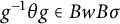 $g^{-1}\theta g\in BwB\sigma $
with
 $\ell (w)>\ell (w_1w_0)$
, which contradicts the fact that
 $\operatorname {{\mathrm {Typ}}}(\theta )=\wp $
. A useful observation is that if
 $w=s_{\varphi }v$
with
 $v\in W_1$
, then
 $\ell (w)=\ell (s_{\varphi })+\ell (v)$
(because
 $s_{\varphi }=w_1w_0=w_0w_1$
). We now proceed with the analysis.
Claim 1: We have
 $u\in U_{\Phi \backslash \Phi _1}^+$
. Write
 $u=u_1u_2$
with
 $u_1\in U_{\Phi _1}^+$
and
 $u_2\in U_{\Phi \backslash \Phi _1}^+$
. Then,
 $$ \begin{align*}w_{1}^{-1}\theta w_{1}= x_{-\varphi}(\pm 1)u_1^-u_2^{\prime}h^{\prime}\sigma\quad\text{with}\ u_1^-=w_{1}^{-1}u_1w_{1}\in U_{\Phi_1}^-, u_2^{\prime}\in U_{\Phi\backslash\Phi_1}^+, h^{\prime}\in H. \end{align*} $$
Because
 $u_1^-\in BW_{1}B$
, we have
 $u_1^-\in BvB$
for some
 $v\in W_{1}$
. But because
 $\ell (s_{\varphi }v)=\ell (s_{\varphi })+\ell (v)$
, we have
 $$ \begin{align*}w_{1}^{-1}\theta w_{1}\in Bs_{\varphi}B\cdot BvB\sigma=Bs_{\varphi}vB\sigma, \end{align*} $$
and so
 $v=1$
(as
 $\operatorname {{\mathrm {disp}}}(\theta )=\ell (s_{\varphi })$
). So
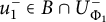 $u_1^-\in B\cap U_{\Phi _1}^-$
, and so
 $u_1^-=1$
; hence,
 $u_1=1$
.
Claim 2: We have
 $h=h_{\omega }(c)$
for some
 $c\in \mathbb {F}^{\times }$
. Write
 $h=h_{\omega _1}(c_1)\cdots h_{\omega _n}(c_n)$
. Let
 $i\neq i_0$
. Then,
 $$ \begin{align*}x_{-\alpha_i}(-1)\theta x_{-\alpha_i}(1)=x_{-\varphi}(1)x_{-\alpha_i}(-1)ux_{-\alpha_i}(c_i^{-1})h\sigma=x_{-\varphi}(1)x_{-\alpha_i}(c_i^{-1}-1)u^{\prime}h\sigma, \end{align*} $$
with
 $u^{\prime }\in U^+$
(here, we have used the fact, from Claim 1, that
 $x_{\alpha _i}(a)$
does not appear as a factor in u). Thus, if
 $c_i\neq 1$
, the folding relation gives
 $$ \begin{align*}x_{-\alpha_i}(-1)\theta x_{-\alpha_i}(1)\in Bs_{\varphi}B\cdot Bs_iB\sigma=Bs_{\varphi}s_iB\sigma, \end{align*} $$
a contradiction as before. Hence,
 $c_i=1$
for all
 $i\neq i_0$
, and hence the claim.
Claim 3: We have
 $\sigma =\mathrm {id}$
. Suppose not. Let
 $i\neq i_0$
, and let
 $a\in \mathbb {F}$
with
 $a^{\sigma }\neq a$
. Then,
 $$ \begin{align*}h_{\alpha_i^{\vee}}(a)^{-1}\theta h_{\alpha_i^{\vee}}(a)=x_{-\varphi}(1)uh_{\omega_i}(c)h_{\alpha_i^{\vee}}(a^{\sigma}a^{-1})\sigma. \end{align*} $$
Claim 2 now gives a contradiction.
Claim 4: We have
 $u\in U_{\varphi }$
. Suppose not, and write
 $\theta =x_{-\varphi }(1)uh_{\omega }(c)$
with
 $ u=x_{\beta _k}(a_k)\cdots x_{\beta _1}(a_1) $
in decreasing root height. By assumption,
 $\beta _1\neq \varphi $
. If
 $\beta _1\neq \pi $
(the polar simple root), then there exists
 $\alpha \in \Phi _1^+$
with
 $\beta _1-\alpha \in \Phi ^+$
. Then,
 $$ \begin{align*}x_{-\alpha}(-b)ux_{-\alpha}(b)=u^{\prime}x_{\beta_1-\alpha}(\pm a_1b), \end{align*} $$
with
 $u^{\prime }$
a product of roots in
 $\Phi ^+\backslash \Phi _1$
of height at least
 $\mathrm {ht}(\beta _1-\alpha )$
. Continuing in this way, there exists an element
 $g\in U_{\Phi _1}^-$
with
 $$ \begin{align*}g^{-1}ug=u^{\prime}x_{\pi+\pi^{\prime}}(b)x_{\pi}(a)\quad\text{with}\ a\neq 0\ \text{and}\ b\in \mathbb{F}, \end{align*} $$
where
 $u^{\prime }$
is a product of elements
 $x_{\beta }(\cdot )$
with
 $\beta \in \Phi ^+\backslash (\Phi _1\cup \{\pi ,\pi +\pi ^{\prime }\})$
. We have
 $g^{-1}x_{-\varphi }(1)g=x_{-\varphi }(1)$
(as
 $-\varphi +\alpha \notin \Phi $
for all
 $\alpha \in \Phi _1$
), and
 $h_{\omega }(c)gh_{\omega }(c)^{-1}=g$
(as
 $\langle \omega ,\alpha \rangle =0$
for all
 $\alpha \in \Phi _1$
), and hence
 $$ \begin{align*} g^{-1}\theta g&=g^{-1}x_{-\varphi}(1)uh_{\omega}(c)g=x_{-\varphi}(1)g^{-1}ugh_{\omega}(c)=x_{-\varphi}(1)u^{\prime}x_{\pi+\pi^{\prime}}(b)x_{\pi}(a)h_{\omega}(c). \end{align*} $$
Let
 $d\in \mathbb {F}$
with
 $d\neq 0$
, and write
 $g_1=x_{-\pi -\pi ^{\prime }}(d)$
. Then,
 $$ \begin{align*} Bg_1^{-1}g^{-1}\theta gg_1B&=Bx_{-\pi-\pi^{\prime}}(-d)x_{-\varphi}(1)u^{\prime}x_{\pi+\pi^{\prime}}(b)x_{\pi}(a)h_{\omega}(c)x_{-\pi-\pi^{\prime}}(d)B\\ &= Bx_{-\varphi}(1)x_{-\pi-\pi^{\prime}}(-d)u^{\prime}x_{\pi+\pi^{\prime}}(b)x_{\pi}(a)x_{-\pi-\pi^{\prime}}(dc^{-1})B\\ &= Bx_{-\varphi}(1)x_{-\pi-\pi^{\prime}}(-d)u^{\prime}x_{\pi+\pi^{\prime}}(b)x_{-\pi-\pi^{\prime}}(dc^{-1})x_{-\pi^{\prime}}(\pm adc^{-1})B, \end{align*} $$
where we have used the commutator relation
 $$ \begin{align*}x_{\pi}(a)x_{-\pi-\pi^{\prime}}(dc^{-1})=x_{-\pi-\pi^{\prime}}(dc^{-1})x_{-\pi^{\prime}}(\pm adc^{-1})x_{\pi}(a).\end{align*} $$
Note that
 $$ \begin{align*} u^{\prime}x_{\pi+\pi^{\prime}}(b)x_{-\pi-\pi^{\prime}}(dc^{-1})=x_{\pi+\pi^{\prime}}(b)x_{-\pi-\pi^{\prime}}(dc^{-1})u''\quad\text{where}\ u''\in U^+ \end{align*} $$
(this follows from the fact that
 $u'$
is a product of elements
 $x_{\beta }(\cdot )$
with
 $\beta \in \Phi ^+\backslash (\Phi _1\cup \{\pi ,\pi +\pi '\})$
, and for such
 $\beta $
, if
 $\beta -\pi -\pi '\in \Phi $
, then
 $\beta -\pi -\pi '\in \Phi ^+$
). Therefore,
 $$ \begin{align*} Bg_1^{-1}g^{-1}\theta gg_1B&=Bx_{-\varphi}(1)x_{-\pi-\pi'}(-d)x_{\pi+\pi'}(b)x_{-\pi-\pi'}(dc^{-1})u''x_{-\pi'}(\pm adc^{-1})B\\ &=Bs_{\varphi}x_{\varphi}(1)x_{-\pi-\pi'}(-d)x_{\pi+\pi'}(b)x_{-\pi-\pi'}(dc^{-1})u''x_{-\pi'}(\pm adc^{-1})B. \end{align*} $$
From the commutator relations, we have
 $$ \begin{align*} &x_{\varphi}(1)x_{-\pi-\pi'}(-d)x_{\pi+\pi'}(b)x_{-\pi-\pi'}(dc^{-1})\\ &\quad x_{-\pi-\pi'}(-d)x_{\pi+\pi'}(b)x_{-\pi-\pi'}(dc^{-1})x_{\varphi-\pi-\pi'}(a')x_{\varphi}(b') \end{align*} $$
for some
 $a',b'\in \mathbb {F}$
, and hence
 $$ \begin{align*} Bg_1^{-1}g^{-1}\theta gg_1B&= Bs_{\varphi}x_{-\pi-\pi'}(-d)x_{\pi+\pi'}(b)x_{-\pi-\pi'}(dc^{-1})u'''x_{-\pi'}(\pm adc^{-1})B \end{align*} $$
for some
 $u'''\in U^+$
.
There are now two cases to consider. If
 $b=0$
, then, because
 $s_{\varphi }(-\pi -\pi ')\in \Phi ^+$
, we have
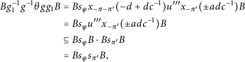 $$ \begin{align*} Bg_1^{-1}g^{-1}\theta gg_1B&= Bs_{\varphi}x_{-\pi-\pi'}(-d+dc^{-1})u'''x_{-\pi'}(\pm adc^{-1})B\\ &=Bs_{\varphi}u'''x_{-\pi'}(\pm adc^{-1})B\\ &\subseteq Bs_{\varphi}B\cdot Bs_{\pi'}B\\ &=Bs_{\varphi}s_{\pi'}B, \end{align*} $$
a contradiction. If
 $b\neq 0$
, then, again using
 $s_{\varphi }(-\pi -\pi ')\in \Phi ^+$
, we have
 $Bs_{\varphi }x_{-\pi -\pi '}(-d)=Bs_{\varphi }x_{-\pi -\pi '}(dc^{-1})$
, and so
 $$ \begin{align*} Bg_1^{-1}g^{-1}\theta gg_1B&= Bs_{\varphi}x_{-\pi-\pi'}(dc^{-1})x_{\pi+\pi'}(b)x_{-\pi-\pi'}(dc^{-1})u'''x_{-\pi'}(\pm adc^{-1})B. \end{align*} $$
Choosing
 $d=-b^{-1}c$
gives
 $Bs_{\varphi }x_{-\pi -\pi '}(dc^{-1})x_{\pi +\pi '}(b)x_{-\pi -\pi '}(dc^{-1})=Bs_{\varphi }s_{\pi +\pi '}$
, and hence
 $$ \begin{align*} Bg_1^{-1}g^{-1}\theta gg_1B&= Bs_{\varphi}s_{\pi+\pi'}u'''x_{-\pi'}(\pm adc^{-1})B\subseteq Bs_{\varphi}s_{\pi+\pi'}B\cdot Bs_{\pi'}B. \end{align*} $$
We have
 $\Phi (s_{\varphi }s_{\pi +\pi '})=(\Phi (s_{\varphi })\backslash \{\varphi ,\varphi -\pi \})\cup \{\pi '\}$
, and it follows that
 $\ell (s_{\varphi }s_{\pi +\pi '})=\ell (s_{\varphi })-1$
and
 $\ell (s_{\varphi }s_{\pi +\pi '}s_{\pi '})=\ell (s_{\varphi })$
. Thus,
 $$ \begin{align*} Bg_1^{-1}g^{-1}\theta gg_1B&=Bs_{\varphi}s_{\pi+\pi'}s_{\pi'}B. \end{align*} $$
Thus, the chamber
 $gg_1B$
is mapped to distance
 $\ell (s_{\varphi })$
by
 $\theta $
, contradicting the second sentence of the proof (as
 $s_{\varphi }s_{\pi +\pi '}s_{\pi '}\neq s_{\varphi }$
). This completes the proof of the claim.
Claim 5: We have
 $\theta =x_{-\varphi }(1)x_{\varphi }(-(c-1)^2)h_{\omega }(c)$
for some
 $c\in \mathbb {F}^{\times }$
. From Claims 1–4, we have
 $$ \begin{align*}\theta=x_{-\varphi}(1)x_{\varphi}(a)h_{\omega}(c)\quad\text{for some}\ a\in \mathbb{F}\ \text{and}\ c\in\mathbb{F}^{\times}. \end{align*} $$
We will now make a careful commutator relation calculation, using the consistent sign conventions:
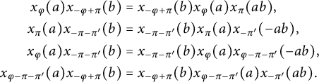 $$ \begin{align*} x_{\varphi}(a)x_{-\varphi+\pi}(b)&=x_{-\varphi+\pi}(b)x_{\varphi}(a)x_{\pi}(ab),\\ x_{\pi}(a)x_{-\pi-\pi'}(b)&=x_{-\pi-\pi'}(b)x_{\pi}(a)x_{-\pi'}(-ab),\\ x_{\varphi}(a)x_{-\pi-\pi'}(b)&=x_{-\pi-\pi'}(b)x_{\varphi}(a)x_{\varphi-\pi-\pi'}(-ab),\\ x_{\varphi-\pi-\pi'}(a)x_{-\varphi+\pi}(b)&=x_{-\varphi+\pi}(b)x_{\varphi-\pi-\pi'}(a)x_{-\pi'}(ab). \end{align*} $$
Let
 $g=x_{-\varphi +\pi }(1)x_{-\pi -\pi '}(1)$
. Then,
 $$ \begin{align*} Bg^{-1}\theta gB&=Bx_{-\pi-\pi'}(-1)x_{-\varphi+\pi}(-1)x_{-\varphi}(1)x_{\varphi}(a)h_{\omega}(c)x_{-\varphi+\pi}(1)x_{-\pi-\pi'}(1)B\\ &=Bx_{-\varphi}(1)x_{-\pi-\pi'}(-1)x_{-\varphi+\pi}(-1)x_{\varphi}(a)x_{-\varphi+\pi}(c^{-1})x_{-\pi-\pi'}(c^{-1})B\\ &= Bs_{\varphi}x_{\varphi}(1)x_{-\pi-\pi'}(-1)x_{-\varphi+\pi}(c^{-1}-1)x_{\varphi}(a)x_{\pi}(ac^{-1})x_{-\pi-\pi'}(c^{-1})B. \end{align*} $$
We have
 $$ \begin{align*} x_{\varphi}(a)x_{\pi}(ac^{-1})x_{-\pi-\pi'}(c^{-1})B&=x_{\varphi}(a)x_{-\pi-\pi'}(c^{-1})x_{-\pi'}(-ac^{-2})B\\ &=x_{-\pi-\pi'}(c^{-1})x_{\varphi}(a)x_{\varphi-\pi-\pi'}(-ac^{-1})x_{-\pi'}(-ac^{-2})B\\ &=x_{-\pi-\pi'}(c^{-1})x_{\varphi}(a)x_{-\pi'}(-ac^{-2})B\\ &=x_{-\pi-\pi'}(c^{-1})x_{-\pi'}(-ac^{-2})B, \end{align*} $$
and hence
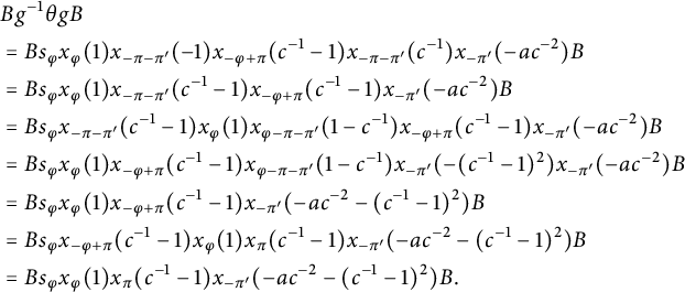 $$ \begin{align*} &Bg^{-1}\theta gB\\ &= Bs_{\varphi}x_{\varphi}(1)x_{-\pi-\pi'}(-1)x_{-\varphi+\pi}(c^{-1}-1)x_{-\pi-\pi'}(c^{-1})x_{-\pi'}(-ac^{-2})B\\ &= Bs_{\varphi}x_{\varphi}(1)x_{-\pi-\pi'}(c^{-1}-1)x_{-\varphi+\pi}(c^{-1}-1)x_{-\pi'}(-ac^{-2})B\\ &= Bs_{\varphi}x_{-\pi-\pi'}(c^{-1}-1)x_{\varphi}(1)x_{\varphi-\pi-\pi'}(1-c^{-1})x_{-\varphi+\pi}(c^{-1}-1)x_{-\pi'}(-ac^{-2})B\\ &= Bs_{\varphi}x_{\varphi}(1)x_{-\varphi+\pi}(c^{-1}-1)x_{\varphi-\pi-\pi'}(1-c^{-1})x_{-\pi'}(-(c^{-1}-1)^2)x_{-\pi'}(-ac^{-2})B\\ &= Bs_{\varphi}x_{\varphi}(1)x_{-\varphi+\pi}(c^{-1}-1)x_{-\pi'}(-ac^{-2}-(c^{-1}-1)^2)B\\ &= Bs_{\varphi}x_{-\varphi+\pi}(c^{-1}-1)x_{\varphi}(1)x_{\pi}(c^{-1}-1)x_{-\pi'}(-ac^{-2}-(c^{-1}-1)^2)B\\ &= Bs_{\varphi}x_{\varphi}(1)x_{\pi}(c^{-1}-1)x_{-\pi'}(-ac^{-2}-(c^{-1}-1)^2)B. \end{align*} $$
Thus, if
 $ac^{-2}+(c^{-1}-1)^2\neq 0$
, we have
 $$ \begin{align*}Bg^{-1}\theta gB= Bs_{\varphi}B\cdot Bs_{\pi'}B=Bs_{\varphi}s_{\pi'}B, \end{align*} $$
a contradiction. Thus,
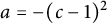 $a=-(c-1)^2$
, completing the proof of the claim.
Claim 6:
 $\theta $
is a long root elation. Let
 $g=x_{\varphi }(-c)x_{-\varphi }(1)s_{\varphi }$
. Then, from Claim 5, we have
 $$ \begin{align*} g\theta g^{-1}&=x_{\varphi}(-c)x_{-\varphi}(1)s_{\varphi}x_{-\varphi}(1)x_{\varphi}(-(c-1)^2)h_{\omega}(c)s_{\varphi}^{-1}x_{-\varphi}(-1)x_{\varphi}(c). \end{align*} $$
Using the relations
 $s_{\varphi }x_{\pm \varphi }(a)s_{\varphi }^{-1}=x_{\mp \varphi }(-a)$
and
 $s_{\varphi }h_{\omega }(c)s_{\varphi }^{-1}=h_{\omega }(c^{-1})$
, we have
 $$ \begin{align*} g\theta g^{-1}&=x_{\varphi}(-c)x_{-\varphi}(1)x_{\varphi}(-1)x_{-\varphi}((c-1)^2)h_{\omega}(c^{-1})x_{-\varphi}(-1)x_{\varphi}(c)\\ &=x_{\varphi}(-c)x_{-\varphi}(1)x_{\varphi}(-1)x_{-\varphi}((c-1)^2)x_{-\varphi}(-c^2)x_{\varphi}(c^{-1})h_{\omega}(c^{-1})\\ &=x_{\varphi}(-c)[x_{-\varphi}(1)x_{\varphi}(-1)x_{-\varphi}(1)]x_{-\varphi}(-2c)x_{\varphi}(c^{-1})h_{\omega}(c^{-1}). \end{align*} $$
Now,
 $x_{-\varphi }(1)x_{\varphi }(-1)x_{-\varphi }(1)=s_{\varphi }(-1)=h_{\omega }(-1)s_{\varphi }$
, and so
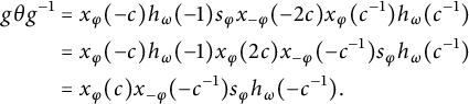 $$ \begin{align*} g\theta g^{-1}&=x_{\varphi}(-c)h_{\omega}(-1)s_{\varphi}x_{-\varphi}(-2c)x_{\varphi}(c^{-1})h_{\omega}(c^{-1})\\ &=x_{\varphi}(-c)h_{\omega}(-1)x_{\varphi}(2c)x_{-\varphi}(-c^{-1})s_{\varphi}h_{\omega}(c^{-1})\\ &=x_{\varphi}(c)x_{-\varphi}(-c^{-1})s_{\varphi}h_{\omega}(-c^{-1}). \end{align*} $$
We have
 $x_{\varphi }(c)x_{-\varphi }(-c^{-1})=s_{\varphi }(c)x_{\varphi }(-c)=h_{\omega }(c)s_{\varphi }x_{\varphi }(-c)=x_{-\varphi }(c^{-1})h_{\omega }(c)s_{\varphi }$
, and because
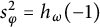 $s_{\varphi }^2=h_{\omega }(-1)$
, we have
 $$ \begin{align*} g\theta g^{-1}&=x_{-\varphi}(c^{-1})h_{\omega}(c)h_{\omega}(-1)h_{\omega}(-c^{-1})=x_{-\varphi}(c^{-1}). \end{align*} $$
Thus,
 $\theta $
is conjugate to the long root elation
 $x_{-\varphi }(c^{-1})$
, completing the proof.▪
3.2 A geometric characterization of root elations for
$\mathsf {E}_6$
and
$\mathsf {E}_7$
buildings


Theorems 3.1 and 3.4 imply an interesting geometric characterization of root elations for types
 $\mathsf {E}_6$
and
 $\mathsf {E}_7$
(see Theorem 3.6 below). In the following lemma, and again in the following subsection, we make use of [Reference Humphreys9, Section 10.3, Lemma B], which says that if
 $\lambda \in P$
is dominant (that is,
 $\lambda \in \mathbb {Z}_{\geq 0}\omega _1+\cdots +\mathbb {Z}_{\geq 0}\omega _n$
), and if
 $w\in W$
with
 $w\lambda =\lambda $
, then
 $w\in W_J$
, where
 $J=\{s\in S\mid s\lambda =\lambda \}$
.
Lemma 3.5 Let
 $i=1$
if
 $\Phi =\mathsf {E}_6$
and
 $i=7$
if
 $\Phi =\mathsf {E}_7$
. Then,
 $s_{\alpha }\in W_i\cup W_is_iW_i$
for all
 $\alpha \in \Phi $
, where
 $W_i$
denotes the parabolic subgroup of the Weyl group generated by
 $S\backslash \{s_i\}$
.
Proof Consider the
 $\Phi =\mathsf {E}_7$
case. Because
 $s_{-\alpha }=s_{\alpha }$
, we may assume that
 $\alpha \in \Phi ^+$
. Let
 $\Phi _7=\{\alpha \in \Phi \mid \langle \alpha ,\omega _7\rangle =0\}$
be the
 $\mathsf {E}_6$
subsystem. If
 $\alpha \in \Phi _7^+$
, then, because
 $W_7$
is transitive on
 $\Phi _7$
, we have
 $\alpha =w\alpha _1$
for some
 $w\in W_7$
, and hence
 $s_{\alpha }=ws_1w^{-1}\in W_7$
. If
 $\alpha \in \Phi ^+\backslash \Phi _7$
, then we claim that
 $\alpha \in W_7\cdot \alpha _7$
, from which it follows that
 $s_{\alpha }\in W_7s_7W_7$
. To see this, note that
 $\alpha _7=-\omega _6+2\omega _7$
, and hence, for
 $w\in W_7$
, we have
 $w\alpha _7=\alpha _7$
if and only if
 $w\omega _6=\omega _6$
(as
 $w\omega _7=\omega _7$
). Because
 $\omega _6$
is dominant (in the space of
 $\mathsf {E}_6$
coweights), it follows from [Reference Humphreys9, Section 10.3, Lemma B] that
 $w\in W_{\mathsf {D}_5}$
(the subgroup of
 $W_7$
generated by
 $s_1,\ldots ,s_5$
). Thus, the stabilizer of
 $\alpha _7$
in
 $W_7$
is
 $W_{\mathsf {D}_5}$
, and so by counting
 $|W_7\cdot \alpha _7|=|W_7|/|W_{\mathsf {D}_5}|=27$
. Clearly each root
 $w\alpha _7$
with
 $w\in W_7$
is in
 $\Phi ^+\backslash \Phi _7$
(as the coefficient of
 $\alpha _7$
is
 $1$
), and because
 $|\Phi ^+\backslash \Phi _7|=63-36=27$
, we conclude that
 $W_7$
is transitive on
 $\Phi ^+\backslash \Phi _7$
, and hence the result. The argument for the
 $\mathsf {E}_6$
case is similar.▪
Theorem 3.6 Let
 $\theta $
be a type preserving automorphism of a thick building
 $\Delta $
. If
 $\Delta $
has type
 $\mathsf {E}_6$
(respectively
 $\mathsf {E}_7$
), then
 $\theta $
is a root elation if and only if each point of the Lie incidence geometry
 $\mathsf {E}_{6,1}(\mathbb {F})$
(respectively
 $\mathsf {E}_{7,7}(\mathbb {F})$
) is either fixed or mapped to a collinear point by
 $\theta $
.
Proof If
 $\theta $
is a root elation, then by Theorem 3.1, we have that
 $\delta (c,c^{\theta })$
is a reflection (or the identity) for all chambers
 $c\in \Delta $
. It follows from Lemma 3.5 that
 $\delta (c,c^{\theta })\in W_i\cup W_is_iW_i$
(with
 $i=1$
in the
 $\mathsf {E}_6$
case and
 $i=7$
in the
 $\mathsf {E}_7$
case). In geometric terms, this says that points of the geometries
 $\mathsf {E}_{6,1}(\mathbb {F})$
and
 $\mathsf {E}_{7,7}(\mathbb {F})$
are either fixed, or are mapped to collinear points (see Lemma 6.2 for another proof, applying to geometries including the
 $\mathsf {E}_{7,7}(\mathbb {F})$
case).
To prove the converse for
 $\mathsf {E}_7$
, note that if each point of
 $\mathsf {E}_{7,7}(\mathbb {F})$
is either fixed or mapped to a collinear point, then no line of the
 $\mathsf {E}_{7,7}(\mathbb {F})$
geometry is mapped to an opposite line. Thus,
 $\theta $
is
 $\{6\}$
-domestic, and from the classification of admissible diagrams, this forces
 $\theta $
to have the polar diagram. Thus,
 $\theta $
is a root elation by Theorem 3.4.
We now prove the converse for
 $\mathsf {E}_6$
. If nontrivial
 $\theta $
is not a root elation, then
 $\theta $
does not have polar diagram (by Theorem 3.4), and hence, by the classification of admissible diagrams,
 $\theta $
maps a (point,symp)-pair
 $(p,\xi )$
of
 $\mathsf {E}_{6,1}(\mathbb {F})$
to an opposite (here, points are type
 $1$
vertices, and symps are type
 $6$
vertices). Then, because no point of
 $\xi ^\theta $
is collinear to p, the point
 $p^\theta $
is at distance
 $2$
from p, completing the proof.▪
3.3 Distances attained by long root elations
Here, we prove Corollary 3. Let
 $\Delta $
be an irreducible Moufang spherical building other than a generalized octagon, and recall (as in Section 3.1) that one may associate a crystallographic root system
 $\Phi $
to
 $\Delta $
. Let
 $\Phi _r$
denote the associated reduced root system (thus,
 $\Phi _r=\Phi $
if
 $\Phi $
is reduced, and
 $\Phi _r$
is the
 $\mathsf {C}_n$
subsystem consisting of the middle and long length roots in the nonreduced
 $\mathsf {BC}_n$
case). Consider the long root geometry
 $\mathscr {G}$
. Let
 $P=P_{S\backslash \wp }$
be the standard parabolic subgroup of G of type
 $S\backslash \wp $
, and let
 $W'=W_{S\backslash \wp }$
. The points of
 $\mathscr {G}$
are the cosets in
 $G/P$
, and we have
 $ G=\bigsqcup _{w\in R(\wp )}PwP, $
where
 $R(\wp )$
is the set of minimal length double coset representatives for
 $W'\backslash W/W'$
. The Weyl distance
 $\delta (g_1P,g_2P)$
between points
 $g_1P$
and
 $g_2P$
is defined to be the unique element
 $\delta (g_1P,g_2P)=w\in R(\wp )$
with
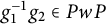 $g_1^{-1}g_2\in PwP$
. Points
 $g_1P$
and
 $g_2P$
are (i) collinear if
 $\delta (g_1P,g_2P)=s$
for some
 $s\in \wp $
(thus, in type
 $\mathsf {A}$
, there are two “flavors” of collinearity), and (ii) opposite if
 $\delta (g_1P,g_2P)=w_{S\backslash \wp }w_0$
. Note that
 $w_{S\backslash \wp }w_0$
is the minimal length representative of
 $W'w_0W'$
, and that
 $w_{S\backslash \wp }w_0=s_{\varphi }$
(by comparing inversion sets).
Theorem 3.7 Let
 $\theta $
be a long root elation of a Moufang spherical building
 $\Delta $
.
-
(1) Suppose that
$\theta $
is not a generalized octagon. Let
$\Phi _r$
be the reduced root system of
$\Delta $
, and let
$\mathscr {G}$
be the long root geometry.-
(a) If
$\Phi _r=\mathsf {C}_n$
with
$n\geq 2$
, or if
$\Phi _r=\mathsf {B}_2$
, then every point of
$\mathscr {G}$
is either fixed, or is mapped onto an opposite point by
$\theta $
. -
(b) In all other cases, every point of
$\mathscr {G}$
is either fixed, mapped onto a collinear point, or mapped onto an opposite point by
$\theta $
.
-
-
(2) Suppose that
$\Delta $
is a Ree–Tits octagon. Then, every point of
$\Delta $
is mapped by
$\theta $
onto a point at distance
$0$
,
$4$
, or
$8$
in the incidence graph.


In particular, for each type, there exists at least one element
 $w\in R(\wp )$
such that no point is mapped onto a point at distance w by
 $\theta $
.
Proof Let
 $W'=W_{S\backslash \wp }$
, and let
 $D(\theta )=\{\delta (gP,\theta gP) \mid gP\in G/P\}\subseteq R(\wp )$
be the set of distances realized by
 $\theta $
. From Theorem 3.1, we see that
 $D(\theta )$
consists precisely of the identity, along with the minimal length representatives of the double cosets
 $W's_{\alpha }W'$
with
 $\alpha $
a long root.
Consider the
 $\mathsf {A}_n$
case. We claim that
 $$ \begin{align} \Phi^+=\Phi_{S\backslash\wp}^+\sqcup(W'\cdot\alpha_1)\sqcup (W'\cdot\alpha_n)\sqcup\{\varphi\}. \end{align} $$
The result follows from this claim, because if
 $\alpha \in \Phi _{S\backslash \wp }^+$
, then
 $s_{\alpha }\in W'$
, if
 $\alpha \in W'\cdot \alpha _1$
, then
 $s_{\alpha }=ws_1w^{-1}$
for some
 $w\in W'$
, and so
 $W's_{\alpha }W'=W's_1W'$
, if
 $\alpha \in W'\cdot \alpha _n$
, then
 $W's_{\alpha }W'=W's_nW'$
, and if
 $\alpha =\varphi $
, then
 $W's_{\alpha }W'=W'w_{S\backslash \wp }w_0W'$
.
To prove (3.2), we first claim that
 $$ \begin{align*} W'\cdot\alpha_1=\{\alpha\in\Phi^+\mid \langle\alpha,\omega_1\rangle=1\text{ and }\langle\alpha,\omega_n\rangle=0\}. \end{align*} $$
Denote the right-hand side by X. If
 $\alpha =w\alpha _1$
with
 $w\in W'$
, then
 $\langle \alpha ,\omega _1\rangle =\langle \alpha _1,w^{-1}\omega _1\rangle =\langle \alpha _1,\omega _1\rangle =1$
, because
 $w^{-1}\omega _1=\omega _1$
for all
 $w\in W'$
. It follows that
 $\alpha \in \Phi ^+$
, and similarly, we have
 $\langle \alpha ,\omega _n\rangle =0$
, and so
 $W'\cdot \alpha _1\subseteq X$
. By the orbit-stabilizer theorem, we have
 $$ \begin{align*}|W'\cdot\alpha_1|=|W'|/|\mathrm{stab}_{W'}(\alpha_1)|=|W_{\mathsf{A}_{n-2}}|/|W_{\mathsf{A}_{n-3}}|=n-1, \end{align*} $$
where the stabilizer computation follows from the fact that if
 $w\in W'$
, then
 $w\alpha _1=\alpha _1$
if and only if
 $w\omega _2=\omega _2$
(as
 $\alpha _1=2\omega _1-\omega _2$
and
 $w\omega _1=\omega _1$
), if and only if
 $w\in W_{S\backslash \{1,2,n\}}$
(by [Reference Humphreys9, Section 10.3, Lemma B]). Because
 $|X|=n-1$
, we have
 $W'\cdot \alpha _1=X$
, and hence the claim.
Dually, we have
 $W'\cdot \alpha _n=\{\alpha \in \Phi ^+\mid \langle \alpha ,\omega _1\rangle =0\text { and }\langle \alpha ,\omega _n\rangle =1\}$
. Because every positive root
 $\alpha $
either has
 $\langle \alpha ,\omega _1\rangle =\langle \alpha ,\omega _n\rangle =0$
(in which case
 $\alpha \in \Phi _{S\backslash \wp }^+$
), or
 $\langle \alpha ,\omega _1\rangle =1$
and
 $\langle \alpha ,\omega _n\rangle =0$
(in which case
 $\alpha \in W'\cdot \alpha _1$
), or the dual situation (with
 $\alpha \in W'\cdot \alpha _n$
), or
 $\langle \alpha ,\omega _1\rangle =\langle \alpha ,\omega _n\rangle =1$
(in which case
 $\alpha =\varphi $
), the claim (3.2) follows.
Consider the
 $\mathsf {B}_n$
case with
 $n\geq 3$
, and let
 $\Phi _L$
be the set of long roots. Let
 $Y=\{\alpha \in \Phi _L^+\mid \langle \alpha ,\omega _2\rangle =0\}$
and
 $X=\Phi _L^+\backslash (Y\cup \{\varphi \})$
. Thus,
 $\Phi _L^+=X\sqcup Y\sqcup \{\varphi \}$
. If
 $\alpha \in Y$
, then
 $W's_{\alpha }W'=W'$
. By inspection of the root system, we have
 $$ \begin{align*}X=\{\alpha\in\Phi_L^+\mid \langle\alpha,\omega_2\rangle=1\text{ and }\langle\alpha,\omega_n\rangle\in\{0,2\}\}. \end{align*} $$
From this description, it is clear that
 $W'\cdot \alpha _2\subseteq X$
, and a similar orbit-stabilizer calculation as in the
 $\mathsf {A}_n$
case gives
 $X=W'\cdot \alpha _2$
. Hence the result in this case.
The
 $\mathsf {B}_2$
and
 $\mathsf {C}_n$
cases are immediate, as the polar node corresponds to a short root in these cases, and the
 $\mathsf {D}_n$
case is very similar to the
 $\mathsf {B}_n$
case.
Consider the cases
 $\mathsf {E}_n$
(
 $n=6,7,8$
) and
 $\mathsf {F}_4$
. Let
 $\wp =\{p\}$
,
 $Y=\{\alpha \in \Phi _L^+\mid \langle \alpha ,\omega _p\rangle =0\}$
, and
 $X=\Phi _L^+\backslash (Y\cup \{\varphi \})$
. Then,
 $s_{\alpha }\in W'$
for all
 $\alpha \in Y$
, and by inspection of the root systems, we have
 $ X=\{\alpha \in \Phi _L^+\mid \langle \alpha ,\omega _p\rangle =1\}, $
from which it follows that
 $W'\cdot \alpha _p\subseteq X$
. Then,
 $ |W'\cdot \alpha _p|=|W'|/|\mathrm {stab}_{W'}(\alpha _p)|, $
and we compute
 $|\mathrm {stab}_{W'}(\alpha _p)|=|W_{\mathsf {A}_2\times \mathsf {A}_2}|$
,
 $|W_{\mathsf {A}_5}|$
,
 $|W_{\mathsf {E}_6}|$
,
 $|W_{\mathsf {A}_2}|$
in the cases
 $\mathsf {E}_6$
,
 $\mathsf {E}_7$
,
 $\mathsf {E}_8$
,
 $\mathsf {F}_4$
(respectively). For example, in the
 $\mathsf {E}_6$
case, if
 $w\in W'$
, then one has
 $w\alpha _2=\alpha _2$
if and only if
 $w\omega _4=\omega _4$
(as
 $\alpha _2=2\omega _2-\omega _4$
and
 $w\omega _2=\omega _2$
for all
 $w\in W'$
), if and only if
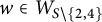 $w\in W_{S\backslash \{2,4\}}$
. Thus,
 $|W'\cdot \alpha _p|=20,32,56,8$
in the cases
 $\mathsf {E}_6$
,
 $\mathsf {E}_7$
,
 $\mathsf {E}_8$
,
 $\mathsf {F}_4$
, and thus
 $W'\cdot \alpha _p=X$
in all cases.
The cases
 $\mathsf {G}_2$
and Ree–Tits octagons are elementary from the geometry of these generalized polygons, because the fixed elements of
 $\theta $
form a ball centered at a point with radius
 $3$
(for
 $\mathsf {G}_2$
) or
 $4$
(for octagons) in the incidence graph.
Finally, we note that in all cases,
 $|D(\theta )|<|R(\wp )|$
, and so there exists at least one
 $w\in R(\wp )$
such that no point is mapped onto distance w by
 $\theta $
. For example, in type
 $\mathsf {A}_n$
, we have
 $|R(\wp )|=7$
and
 $|D(\theta )|=4$
, and in the cases
 $\mathsf {E}_n$
and
 $\mathsf {F}_4$
, we have
 $|R(\wp )|=5$
and
 $|D(\theta )|=3$
.▪
The following corollary stems from a question asked to us by Barbara Baumeister.
Corollary 3.8 Let G be the group of type preserving automorphisms of a Moufang spherical building
 $\Delta $
of type other than
 $\mathsf {A}_n$
. There exists a nontrivial conjugacy class
 $\mathscr {C}$
in G which is not transitive on any vertex type.
Proof Let
 $\mathscr {C}$
be the conjugacy class of long root elations. Consider first the case that opposition is type preserving, and let i be a vertex type. Let x be a type i vertex. If i is not the polar node, then from Theorem 3.1, no element of
 $\mathscr {C}$
maps x to an opposite vertex, and hence
 $\mathscr {C}$
is not transitive on type i vertices. If i is the polar node, then by Theorem 3.7, there is a distance in the long root geometry such that no element of
 $\mathscr {C}$
maps a point of the long root geometry to this distance, and hence the result in this case.
Now suppose that opposition is not type preserving. Thus,
 $\Delta $
is of type
 $\mathsf {D}_{2n+1}$
or
 $\mathsf {E}_6$
. Consider the
 $\mathsf {D}_{2n+1}$
case. By Theorem 3.1, no vertex of type
 $1,3,4,\ldots ,2n-1$
is mapped to an opposite vertex, and so
 $\mathscr {C}$
is not transitive on these vertex types, and by Theorem
3.7,
 $\mathscr {C}$
is not transitive on the vertices of polar type
 $2$
. It is easy to see, as in Theorem 3.7, that in the
 $\mathsf {D}_{2n+1,2n+1}(\mathbb {F})$
geometry, points are either fixed or mapped to collinear points by long root elations, and similarly in the
 $\mathsf {D}_{2n+1,2n}(\mathbb {F})$
geometry. Thus,
 $\mathscr {C}$
is not transitive on the vertices of type
 $2n$
or
 $2n+1$
either.
Consider the
 $\mathsf {E}_6$
case. As above,
 $\mathscr {C}$
is not transitive on the vertices of type
 $2$
or
 $4$
. Moreover, because points of the
 $\mathsf {E}_{6,1}(\mathbb {F})$
geometry are either fixed or mapped to collinear points by long root elations (see Theorem 3.6), we see that
 $\mathscr {C}$
is not transitive on vertices of type
 $1$
, or dually type
 $6$
. Similar calculations show that in the
 $\mathsf {E}_{6,3}(\mathbb {F})$
geometry, a long root elation either fixes points, maps them to collinear points, or maps them to distance
 $s_{\varphi _{\mathsf {D}_5}}$
(with the
 $\mathsf {D}_5$
system generated by
 $\alpha _1,\ldots ,\alpha _5$
). Thus,
 $\mathscr {C}$
is not transitive on any vertex type.▪
Remark 3.9 In the
 $\mathsf {A}_n$
case, the class
 $\mathscr {C}$
of long root elations is transitive on vertices of types
 $1$
and n, and is not transitive on any other vertex types.
3.4 Short root elations
We now record the situation for short root elations of split buildings. In this case, there is some dependence on the characteristic of the underlying field. The proof for the
 $\mathsf {F}_4$
case is postponed to Section 7. For
 $i\leq n$
, let
 $\mathsf {B}_{n;i}^1$
(respectively
 $\mathsf {C}_{n;i}^1$
) denote the admissible
 $\mathsf {B}_n$
(respectively
 $\mathsf {C}_n$
) diagram
 $(\Gamma ,\{1,\ldots ,i\},\mathrm {id})$
.
Theorem 3.10 Let
 $\theta \in U_{\alpha }\backslash \{1\}$
for some short root
 $\alpha $
.
-
(1) If
$\Phi =\mathsf {B}_n$
, then
$\theta $
has opposition diagram
$\mathsf {B}_{n;2}^1$
if
$\mathrm {char}(\mathbb {F})\neq 2$
, and
$\mathsf {B}_{n;1}^1$
if
$\mathrm {char}(\mathbb {F})=2$
. -
(2) If
$\Phi =\mathsf {C}_n$
, then
$\theta $
has opposition diagram
$\mathsf {C}_{n;2}^1$
if
$\mathrm {char}(\mathbb {F})\neq 2$
, and
$\mathsf {C}_{n;1}^2$
if
$\mathrm {char}(\mathbb {F})=2$
. -
(3) If
$\Phi =\mathsf {F}_4$
, then
$\theta $
has opposition diagram
$\mathsf {F}_{4;2}$
if
$\mathrm {char}(\mathbb {F})\neq 2$
, and
$\mathsf {F}_{4;1}^4$
if
$\mathrm {char}(\mathbb {F})=2$
. -
(4) If
$\Phi =\mathsf {G}_2$
, then
$\theta $
has opposition diagram
$\mathsf {G}_{2;2}$
if
$\mathrm {char}(\mathbb {F})\neq 3$
, and
$\mathsf {G}_{2;1}^1$
if
$\mathrm {char}(\mathbb {F})=3$
.


In particular, with the exception of the cases
 $\Phi =\mathsf {B}_2$
and
 $\Phi =\mathsf {C}_2$
with
 $\mathrm {char}(\mathbb {F})\neq 2$
, and
 $\Phi =\mathsf {G}_2$
with
 $\mathrm {char}(\mathbb {F})\neq 3$
, the collineation
 $\theta $
is domestic.
Proof The statements for the polar spaces
 $\mathsf {B}_n$
and
 $\mathsf {C}_n$
are easily proved using the matrix descriptions of these groups, and we omit the details.
Consider the case
 $\Phi =\mathsf {F}_4$
. If
 $\mathrm {char}(\mathbb {F})=2$
, then the
 $\mathsf {F}_{4,4}(\mathbb {F})$
geometry isometrically embeds into the
 $\mathsf {F}_{4,1}(\mathbb {F})$
geometry (surjectively if
 $\mathbb {F}$
is perfect), with short root elations becoming long root elations, and so Theorem 3.1 implies that the opposition diagram of
 $\theta $
is
 $\mathsf {F}_{4;1}^4$
. The proof for the case
 $\mathrm {char}(\mathbb {F})\neq 2$
is postponed until Corollary 7.7.
Consider the case
 $\Phi =\mathsf {G}_2$
. If
 $\mathrm {char}(\mathbb {F})=3$
, then, as in the
 $\mathsf {F}_4$
case, we have opposition diagram
 $\mathsf {G}_{2,1}^1$
. Thus, suppose that
 $\mathrm {char}(\mathbb {F})\neq 3$
. A direct calculation shows that
 $$ \begin{align*}Bw_0^{-1}x_{\alpha_1+\alpha_2}(1)^{-1}x_{\varphi'}(a)x_{\alpha_1+\alpha_2}(1)w_0B=Bw_0B, \end{align*} $$
and so
 $\theta $
is not domestic, completing the proof.▪
One can also show that the class
 $\mathscr {C}$
of short root elations in split type
 $\mathsf {F}_4$
gives another class not transitive on any vertex type (cf. Corollary 3.8).
Corollary 3.11 The class
 $\mathscr {C}$
of short root elations of
 $\mathsf {F}_4(\mathbb {F})$
does not act transitively on the set of type i vertices, for each
 $i=1,2,3,4$
.
Proof If
 $\mathrm {char}(\mathbb {F})=2$
, then the
 $\mathsf {F}_{4,4}(\mathbb {F})$
geometry isometrically embeds into the
 $\mathsf {F}_{4,1}(\mathbb {F})$
geometry, with short root elations becoming long root elations, and hence the result. Suppose that
 $\mathrm {char}(\mathbb {F})\neq 2$
. As in the proof of Corollary 3.8, it is sufficient to show that for each
 $i=1,2,3,4$
, there exists at least one distance such that no point of the geometry
 $\mathsf {F}_{4,i}(\mathbb {F})$
is mapped to this distance by a short root elation
 $\theta $
. By Theorem 3.10, no vertices of type
 $2$
or
 $3$
are mapped onto opposite vertices, and so it remains to consider vertices of types
 $1$
and
 $4$
.
After conjugating, we may assume that
 $\theta =x_{\varphi '}(1)$
, where
 $\varphi '$
is the highest short root. As in Section 2.5, let
 $M_1$
denote the set of minimal length coset representatives of cosets in
 $W/W_1$
(recall the notation (2.5)), and let
 $R_1$
denote the set of minimal length representatives for the double cosets in
 $W_1\backslash W/W_1$
. Each vertex of type
 $1$
is of the form
 $x=uvP_1$
,
 $v\in M_1$
, and
 $u\in U_{\Phi (v)}^+$
, and the distance between x and
 $x^{\theta }$
is the unique element
 $w\in R_1$
such that
 $v^{-1}u^{-1}\theta uv\in P_1wP_1$
.
For any
 $u\in U^+$
, we have, by commutator relations,
 $$ \begin{align*}u^{-1}\theta u=u^{-1}x_{\varphi'}(1)u=x_{\alpha}(a)x_{\beta}(b)x_{\gamma}(c)x_{\delta}(d), \end{align*} $$
for some
 $a,b,c,d\in \mathbb {F}$
, where
 $\alpha ,\beta ,\gamma ,\delta $
are the unique roots of heights
 $8,9,10,11$
. Explicitly, these roots are
 $\varphi '$
,
 $\varphi '+\alpha _3$
,
 $\varphi '+\alpha _2+\alpha _3$
, and
 $\varphi $
, and because the corresponding root subgroups commute with each other, the order in the above product is irrelevant.
It follows that
 $$ \begin{align*}v^{-1}u^{-1}\theta uv=x_{v^{-1}\alpha}(a)x_{v^{-1}\beta}(b)x_{v^{-1}\gamma}(c)x_{v^{-1}\delta}(d), \end{align*} $$
for some
 $a,b,c,d\in \mathbb {F}$
. If either
 $v^{-1}\alpha \in \Phi ^+$
or
 $v^{-1}\alpha \in \Phi _1$
(where
 $\Phi _1$
is generated by
 $\alpha _2,\alpha _3,\alpha _4$
), then
 $x_{v^{-1}\alpha }(a)\in P_1$
, and hence can be ignored as we are interested in
 $P_1$
-double cosets. Similarly, for the other terms (as they pairwise commute). By a direct calculation (using
 $\mathsf {MAGMA}$
), for all
 $v\in M_1$
, it turns out that
 $$ \begin{align*}\{v^{-1}\alpha,v^{-1}\beta,v^{-1}\gamma,v^{-1}\delta\}\cap (\Phi^-\backslash\Phi_1)\subseteq \{-(1000),-(1100),-(1110),-(2342)\}. \end{align*} $$
It therefore suffices to consider
 $P_1gP_1$
, where
 $$ \begin{align*}g=x_{-(2342)}(a)x_{-(1110)}(b)x_{-(1100)}(c)x_{-(1000)}(d)\quad\text{with}\ a,b,c,d\in\mathbb{F}. \end{align*} $$
A straightforward calculation, using the folding relation, gives
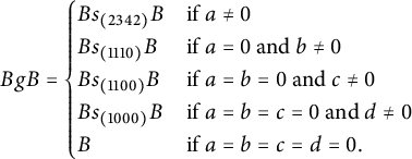 $$ \begin{align*} BgB=\begin{cases} Bs_{(2342)}B&\text{if}\ a\neq 0\\ Bs_{(1110)}B&\text{if}\ a= 0\ \text{and}\ b\neq 0\\ Bs_{(1100)}B&\text{if}\ a=b=0\ \text{and}\ c\neq 0\\ Bs_{(1000)}B&\text{if}\ a=b=c=0\ \text{and}\ d\neq 0\\ B&\text{if}\ a=b=c=d=0. \end{cases} \end{align*} $$
Because
 $P_1s_{(1100)}P_1=P_1s_{(1000)}P_1=P_1s_1P_1$
, and
 $s_{(1110)}=s_1s_2s_3s_2s_1$
, it follows that
 $$ \begin{align*}P_1gP_1\in \{P_1,P_1s_1P_1,P_1s_1s_2s_3s_2s_1P_1,P_1s_{\varphi}P_1\}. \end{align*} $$
In the language of parapolar spaces, this means that every point of
 $\mathsf {F}_{4,1}(\mathbb {F})$
is either fixed, mapped to a collinear point, mapped to a symplectic point, or mapped to an opposite point by
 $\theta $
. In particular, no point is mapped to a point at special distance
 $s_1s_2s_3s_2s_4s_3s_2s_1$
(see Section 2.5), and hence
 $\mathscr {C}$
is not transitive on type
 $1$
vertices. The arguments for type
 $4$
vertices are entirely analogous.▪
4 Unipotent elements
Let
 $\Delta $
be a split irreducible spherical building of exceptional type with root system
 $\Phi $
. In this section, we give an extension of Theorem 3.1, showing that every “polar closed” (see below) type preserving admissible Dynkin diagram of type
 $\Phi $
can be realized as the opposition diagram of a unipotent element
 $u\in U^+$
. In fact, we show that these are precisely the diagrams that arise as opposition diagrams of elements in
 $U^+$
(for nonspecial characteristic).
Let
 $\mathsf {X}$
be a type preserving admissible Dynkin diagram, and let
 $\mathsf {X}=\mathsf {X}_0,\mathsf {X}_1,\ldots $
be subdiagrams such that, for
 $j\geq 1$
, the diagram
 $\mathsf {X}_{j}$
is obtained from
 $\mathsf {X}_{j-1}$
by removing an encircled polar type from one of the connected components of
 $\mathsf {X}_{j-1}$
. Suppose that this process terminates at step
 $j=k$
(that is,
 $\mathsf {X}_k$
has no polar nodes encircled). We say that a type preserving diagram
 $\mathsf {X}$
is polar closed if
 $\mathsf {X}_k$
is an empty diagram (that is, has no nodes encircled).
For example, the following diagrams are polar closed:
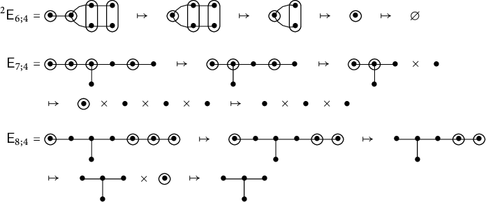
whereas the diagrams
 $\mathsf {F}_{4;1}^4$
and
 $\mathsf {G}_{2;1}^1$
are not polar closed (as the polar node is not encircled). Indeed, by direct inspection of the list of admissible diagrams, these two diagrams are the only nonpolar closed diagrams of exceptional type.
Suppose that
 $\mathsf {X}$
is polar closed. Thus, one may define diagrams
 $\mathsf {X}_0,\ldots ,\mathsf {X}_k$
by successively removing encircled polar types, until no polar nodes are encircled, and
 $\mathsf {X}_k$
is an empty diagram. Let
 $\varphi _1,\ldots ,\varphi _k\in \Phi ^+$
be the highest roots removed at each stage. For example, the highest roots corresponding to the three polar closed diagrams above are:
 $$ \begin{align*} \varphi_{\mathsf{E}_6}&=(122321)\mapsto\varphi_{\mathsf{A}_5}=(101111)\mapsto\varphi_{\mathsf{A}_3}=(001110)\mapsto\varphi_{\mathsf{A}_1}=(000100),\\ \varphi_{\mathsf{E}_7}&=(2234321)\mapsto\varphi_{\mathsf{D}_6}=(0112221)\mapsto\varphi_{\mathsf{D}_4}=(0112100)\mapsto\varphi_{\mathsf{A}_1}=(0010000),\\ \varphi_{\mathsf{E}_8}&=(23465432)\mapsto \varphi_{\mathsf{E}_7}=(22343210)\mapsto\varphi_{\mathsf{D}_6}=(01122210)\mapsto\varphi_{\mathsf{A}_1}=(00000010). \end{align*} $$
In general, the sequence of diagrams
 $\mathsf {X}_0,\ldots ,\mathsf {X}_k$
is not unique (for example, starting with the diagram
 $\mathsf {E}_{7;7}$
, we have
 $\mathsf {E}_{7;7}\mapsto \mathsf {D}_{6;6}\mapsto \mathsf {D}_{5;5}\times \mathsf {A}_{1;1}$
, from which point one may choose to remove either the polar node of the
 $\mathsf {D}_5$
component, or the
 $\mathsf {A}_1$
component). However, it is clear that the set
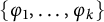 $\{\varphi _1,\ldots ,\varphi _k\}$
of highest roots obtained is independent of the choices made. Moreover, note that these roots are mutually perpendicular (by definition of the polar type), and hence the subgroup
 $U(\mathsf {X})$
of G generated by the root subgroups
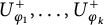 $U_{\varphi _1}^+,\ldots ,U_{\varphi _k}^+$
is abelian. We call an element
 $g\in U(\mathsf {X})$
generic if
 $$ \begin{align*}g=x_{\varphi_1}(a_1)\cdots x_{\varphi_k}(a_k)\quad\text{with}\ a_1,\ldots,a_k\neq 0. \end{align*} $$
Let the dual polar node of a Dynkin diagram be the subset
 $\wp ^{\prime }\subseteq S$
corresponding to the polar node of the dual diagram. Thus,
 $\wp ^{\prime }=\wp $
in the simply laced case, and
 $\wp ^{\prime }=\{1\},\{2\},\{4\},\{1\}$
in the cases
 $\Phi =\mathsf {B}_n,\mathsf {C}_n,\mathsf {F}_4,\mathsf {G}_2$
, respectively. We call a type preserving admissible diagram
 $\mathsf {X}$
dual polar closed if the above algorithm, with each occurrence of “polar node” replaced by “dual polar node,” terminates in an empty diagram. Let
 $\varphi _1^{\prime },\ldots ,\varphi _{\ell }^{\prime }\in \Phi ^+$
denote the sequence of highest short roots obtained in an analogous way. In the case of special characteristic, the subgroup
 $U(\mathsf {X})^{\prime }$
of
 $G_{\Phi }(\mathbb {F})$
generated by
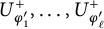 $U_{\varphi _1^{\prime }}^+,\ldots , U_{\varphi _{\ell }^{\prime }}^+$
is commutative. We define a generic element of
 $U(\mathsf {X})^{\prime }$
in an analogous way. By inspection, note that if
 $\mathsf {X}$
is type preserving and is not polar closed, then
 $\mathsf {X}$
is necessarily dual polar closed.
In this section, we prove the following theorem.
Theorem 4.1 Let
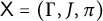 $\mathsf {X}=(\Gamma ,J,\pi )$
be a type preserving admissible Dynkin diagram of exceptional type
 $\Phi $
, and let
 $G=G_{\Phi }(\mathbb {F})$
.
-
(1) Suppose that
$\mathrm {char}(\mathbb {F})$
is not special. Then,
$\mathsf {X}$
is the opposition diagram of an element of
$U^+$
if and only if
$\mathsf {X}$
is polar closed. Moreover, if
$\mathsf {X}$
is polar closed, then each generic element
$\theta \in U(\mathsf {X})$
has opposition diagram
$\mathsf {X}$
. -
(2) Suppose that
$\mathrm {char}(\mathbb {F})$
is special. Then,
$\mathsf {X}$
is the opposition diagram of an element of
$U^+$
. Moreover, if
$\mathsf {X}$
is polar closed, then each generic element
$\theta \in U(\mathsf {X})$
has opposition diagram
$\mathsf {X}$
, and if
$\mathsf {X}$
is dual polar closed, then each generic element
$\theta \in U(\mathsf {X})^{\prime }$
has opposition diagram
$\mathsf {X}$
.


The proof of Theorem 4.1 is given in this section; however, one ingredient—showing that in nonspecial characteristic, the diagrams
 $\mathsf {F}_{4;1}^4$
and
 $\mathsf {G}_{2,1}^1$
are not the opposition diagrams of any element
 $\theta \in U^+$
—will be postponed until latter in the paper (see Theorems 7.1 and 7.10).
Lemma 4.2 Let
 $\Phi $
be of type
 $\mathsf {E}_7$
with highest root
 $\varphi $
. Then,
 $(Bs_{\varphi }B\cdot Bs_{\varphi }B)\cap Bw_0w_{\mathsf {E}_6}B=\emptyset $
.
Proof Write
 $v=w_{\mathsf {D}_5}w_{\mathsf {E}_6}$
(where
 $\mathsf {D}_5$
is generated by
 $\{s_2,s_3,s_4,s_5,s_6\}$
). Because
 $v^{-1}\varphi =\alpha _7$
, we have
 $ v^{-1}s_{\varphi }v=s_{v^{-1}\varphi }=s_{7}, $
and thus
 $s_{\varphi }=vs_7v^{-1}$
. Note that
 $v\in W_7$
(the parabolic subgroup generated by
 $S\backslash \{s_7\}$
). Thus, if
 $w\in W$
is such that
 $$ \begin{align*}BwB\subseteq Bs_{\varphi}B\cdot Bs_{\varphi}B=Bvs_7v^{-1}B\cdot Bvs_7v^{-1}B,\end{align*} $$
then by (2.3) and the deletion condition, there exists a reduced expression for w containing at most two occurrences of the generator
 $s_7$
. However, every reduced expression for
 $y=w_0w_{\mathsf {E}_6}$
contains at least three occurrences of the generator
 $s_7$
. To see this, note that every reduced expression for y must start and end with
 $s_7$
(as it is minimal length in its
 $W_7$
-double coset). It is thus sufficient to show that
 $s_7ys_7$
is not in
 $W_7$
. But we have
 $$ \begin{align*}(s_7ys_7)^{-1}(\varphi_{\mathsf{D}_6})=s_7w_{\mathsf{E}_6}w_{\mathsf{E}_7}\varphi_{\mathsf{D}_6}=-s_7w_{\mathsf{E}_6}\varphi_{\mathsf{D}_6}=-s_7\varphi_{\mathsf{D}_6}=-\varphi_{\mathsf{D}_6}, \end{align*} $$
and so
 $\varphi _{\mathsf {D}_6}\in \Phi (s_7ys_7)$
, and so indeed
 $s_7ys_7\notin W_{7}$
.▪
Remark 4.3 Geometrically, Lemma 4.2 boils down to the following statement in the
 $\mathsf {E}_{7,7}(\mathbb {F})$
geometry (with point set
 $G/P_7$
; recall the notation introduced in Section 2.5): If
 $x,y,z$
are points of
 $\mathsf {E}_{7,7}(\mathbb {F})$
with x and y collinear, and y and z collinear, then x and z are not opposite in
 $\mathsf {E}_{7,7}(\mathbb {F})$
. To make this translation, note that if
 $(Bs_{\varphi }B\cdot Bs_{\varphi }B)\cap Bw_0w_{\mathsf {E}_6}B= \emptyset $
, then, following the above proof, we have
 $(P_7s_7P_7\cdot P_7s_7P_7)\cap P_7w_0P_7= \emptyset $
. Then, note that
 $(P_7s_7P_7\cdot P_7s_7P_7)/P_7$
can be interpreted as the set of points collinear to some point collinear to the base point
 $P_7$
, and
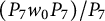 $(P_7w_0P_7)/P_7$
is the set of points opposite the base point
 $P_7$
.
Recall that for roots
 $\alpha ,\beta \in \Phi $
, we write
 $\alpha \leq \beta $
if and only if
 $\beta -\alpha $
is a nonnegative linear combination of simple roots.
Lemma 4.4 Let
 $\Delta $
be an irreducible split spherical building with root system
 $\Phi $
, and suppose that either
 $|\mathbb {F}|>2$
, or that
 $\theta $
is an involution.
-
(1) Suppose that
$\Phi =\mathsf {E}_6$
. If
$\theta \in \langle U_{\alpha }\mid \alpha \geq \alpha _1\rangle $
, then
$\operatorname {{\mathrm {disp}}}(\theta )\leq 30$
. -
(2) Suppose that
$\Phi =\mathsf {E}_7$
, and let
$\varphi _2=\varphi _{\mathsf {D}_6}=(0112221)$
.-
(a) If
$\theta \in \langle U_{\alpha }\mid \alpha \geq \varphi _2\rangle $
, then
$\operatorname {{\mathrm {disp}}}(\theta )\leq 50$
. -
(b) If
$\theta \in \langle U_{\alpha }\mid \alpha \geq \alpha _7\rangle $
, then
$\operatorname {{\mathrm {disp}}}(\theta )\leq 51$
. -
(c) If
$\theta \in \langle U_{\alpha }\mid \alpha \geq \alpha _1\rangle $
, then
$\operatorname {{\mathrm {disp}}}(\theta )\leq 60$
.
-
-
(3) Suppose that
$\Phi =\mathsf {E}_8$
.-
(a) If
$\theta \in \langle U_{\alpha }\mid \operatorname {{\mathrm {ht}}}(\alpha )\geq 23\rangle $
, then
$\operatorname {{\mathrm {disp}}}(\theta )\leq 90$
. -
(b) If
$\theta \in \langle U_{\alpha }\mid \alpha \geq \alpha _8\rangle $
, then
$\operatorname {{\mathrm {disp}}}(\theta )\leq 108$
.
-








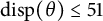







Proof (1) Consider the
 $\mathsf {D}_5$
subsystem generated by
 $\{\alpha _j\mid j\neq 1\}$
. If
 $\alpha \geq \alpha _1$
, then
 $\langle \alpha ,\omega _1\rangle>0$
and so
 $\alpha \in \Phi ^+\backslash \mathsf {D}_5=\Phi (w_0w_{\mathsf {D}_5})$
. Thus, with
 $w_1=w_0w_{\mathsf {D}_5}$
, Proposition 2.8 gives
 $\operatorname {{\mathrm {disp}}}(\theta )\leq 2\ell (w_1)-1=31$
. By the classification of admissible diagrams, this implies that
 $\operatorname {{\mathrm {disp}}}(\theta )\leq 30$
.
(2)(a) We claim that
 $\{\alpha \mid \alpha \geq \varphi _2\}\subseteq \Phi (s_7w_0w_{\mathsf {E}_6})$
. Let
 $\alpha \geq \varphi _2$
. Then,
 $\langle \alpha ,\omega _6\rangle =2$
and
 $\langle \alpha ,\omega _7\rangle =1$
(by inspecting
 $\varphi $
and
 $\varphi _2$
), and because
 $\langle \alpha _i,\alpha _7\rangle =0$
, for
 $i\neq 6,7$
, and
 $\langle \alpha _6,\alpha _7\rangle =-1$
and
 $\langle \alpha _7,\alpha _7\rangle =2$
, it follows that
 $\langle \alpha ,\alpha _7\rangle =0$
. Thus,
 $s_7\alpha =\alpha $
. Writing
 $\alpha =\varphi _2+\beta $
, we have
 $\beta \in \mathsf {E}_6$
(because
 $\langle \varphi _2,\omega _7\rangle =1=\langle \varphi ,\omega _7\rangle $
), and thus, because
 $w_{\mathsf {E}_6}\varphi _2=\varphi _2$
, we have
 $$ \begin{align*}(s_7w_0w_{\mathsf{E}_6})^{-1}\alpha=w_{\mathsf{E}_6}w_0\alpha=-w_{\mathsf{E}_6}\alpha=-w_{\mathsf{E}_6}\varphi_2-w_{\mathsf{E}_6}\beta=-\varphi_2-w_{\mathsf{E}_6}\beta. \end{align*} $$
Because
 $-w_{\mathsf {E}_6}\beta \in \mathsf {E}_6$
, we have
 $\langle -\varphi _2-w_{\mathsf {E}_6}\beta ,\omega _7\rangle =-\langle \varphi _2,\omega _7\rangle =-1$
, and thus
 $(s_7w_0w_{\mathsf {E}_6})^{-1}\alpha \in -\Phi ^+$
.
Thus, by (2.6), we have
 $\operatorname {{\mathrm {disp}}}(\theta )\leq \max \{\ell (w)\mid BwB\subseteq Bw_1B\cdot Bw_1^{-1}B\}$
, where
 $w_1=s_7w_0w_{\mathsf {E}_6}$
. Note that
 $\ell (w_1)=63-37=26$
, and so Proposition 2.8 gives
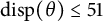 $\operatorname {{\mathrm {disp}}}(\theta )\leq 51$
. It remains to eliminate the possibility of
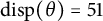 $\operatorname {{\mathrm {disp}}}(\theta )=51$
. By the last sentence in the proof of Proposition 2.8, if
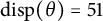 $\operatorname {{\mathrm {disp}}}(\theta )=51$
, then
 $\ell (w_2sw_2^{-1})=51$
, where
 $w_1=w_2s$
with
 $\ell (w_2s)=\ell (w_2)+1$
. Because
 $\ell (w_1s_7)=\ell (w_1)-1$
(as
 $w_1\alpha _7\in -\Phi ^+$
), we can take
 $w_2=w_1s_7$
and
 $s=s_7$
. But then,
 $$ \begin{align*}w_2s_7w_2^{-1}=w_1s_7w_1^{-1}=s_7w_0w_{\mathsf{E}_6}s_7w_{\mathsf{E}_6}w_0s_7=s_{\varphi}, \end{align*} $$
which only has length
 $2\mathrm {ht}(\varphi )-1=33$
, a contradiction.
(2)(b) If
 $\alpha \geq \alpha _7$
, then
 $\alpha \in \Phi ^+\backslash \mathsf {E}_6=\Phi (w_0w_{\mathsf {E}_6})$
. Thus, by Proposition 2.8, we have
 $\operatorname {{\mathrm {disp}}}(\theta )\leq 2\ell (w_0w_{\mathsf {E}_6})-1=2(63-36)-1=53$
. This in turn implies, from the classification of admissible diagrams, that
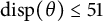 $\operatorname {{\mathrm {disp}}}(\theta )\leq 51$
.
(2)(c) If
 $\alpha \geq \alpha _1$
, then
 $\alpha \in \Phi ^+\backslash \mathsf {D}_6=\Phi (w_0w_{\mathsf {D}_6})$
. Now, note that
 $w_0w_{\mathsf {D}_6}=s_{\varphi }$
. By Lemma 4.2,
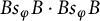 $Bs_{\varphi }B\cdot Bs_{\varphi }B$
does not intersect
 $Bw_0B$
, and so from the proof of Proposition 2.8, we see that
 $\theta $
is domestic. Thus,
 $\operatorname {{\mathrm {disp}}}(\theta )\leq 60$
.
(3)(a) We claim that
 $\{\alpha \mid \operatorname {{\mathrm {ht}}}(\alpha )\geq 23\}\subseteq \Phi (w_1)$
, where
 $w_1 =s_4s_5s_6s_7s_8s_{\varphi }$
(this element has length
 $\ell (s_{\varphi })-5=52$
). Direct calculation shows that each of the elements
 $s_4,s_5,s_6,s_7,s_8$
preserves the set of six roots
 $\{\alpha \in \Phi ^+\mid \mathrm {ht}(\alpha )\geq 23\}$
. Thus, if
 $\operatorname {{\mathrm {ht}}}(\alpha )\geq 23$
, then
 $w_1^{-1}\alpha =s_{\varphi }s_8s_7s_6s_5s_4\alpha =s_{\varphi }\beta $
for some
 $\beta $
with
 $\operatorname {{\mathrm {ht}}}(\beta )\geq 23$
, and thus
 $\langle w_1^{-1}\alpha ,\omega _8\rangle =\langle \beta ,\omega _8\rangle -2\langle \beta ,\varphi \rangle =-\langle \beta ,\omega _8\rangle <0$
(using
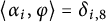 $\langle \alpha _i,\varphi \rangle =\delta _{i,8}$
) and so
 $w_1^{-1}\alpha \in -\Phi ^+$
, hence the claim. It follows from Proposition 2.8 that
 $\operatorname {{\mathrm {disp}}}(\theta )\leq 103$
, and hence, by the classification of admissible diagrams,
 $\operatorname {{\mathrm {disp}}}(\theta )\leq 90$
.
(3)(b) Note that if
 $\alpha \geq \alpha _8$
, then
 $\langle s_{\varphi }\alpha ,\omega _8\rangle =-\langle \alpha ,\omega _8\rangle $
and thus
 $\alpha \in \Phi (s_{\varphi })$
. Because
 $\ell (s_{\varphi })=2\operatorname {{\mathrm {ht}}}(\varphi )-1=57$
, it follows from Proposition 2.8 that
 $\operatorname {{\mathrm {disp}}}(\theta )\leq 113$
, and thus, by the classification of admissible diagrams,
 $\operatorname {{\mathrm {disp}}}(\theta )\leq 108$
.▪
Lemma 4.5 Let
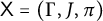 $\mathsf {X}=(\Gamma ,J,\pi )$
be polar closed, and let
 $\varphi _1,\ldots ,\varphi _k$
be the highest roots obtained by the above algorithm. Then,
 $\ell (s_{\varphi _1}\cdots s_{\varphi _k})=\sum _{j=1}^k\ell (s_{\varphi _j})$
and
 $s_{\varphi _1}\cdots s_{\varphi _k}=w_{S\backslash J}w_0$
.
Proof Let
 $\wp _1,\ldots ,\wp _k$
be the polar types. Let
 $S_0=S$
, and define
 $S_j=S_{j-1}\backslash \wp _j$
and
 $\Phi _j=\Phi _{S_j}$
, for
 $j=1,\ldots ,k$
. By (2.1), we have
 $\Phi (s_{\varphi _1})=\Phi _0^+\backslash \Phi _1$
, and it follows by induction that
 $\Phi (s_{\varphi _j})=\Phi _{j-1}^+\backslash \Phi _j$
, for
 $1\leq j\leq k$
. In particular, the inversion sets
 $\Phi (s_{\varphi _1}),\ldots ,\Phi (s_{\varphi _k})$
are disjoint, and thus
 $$ \begin{align*}\Phi(s_{\varphi_1}\cdots s_{\varphi_k})=\bigcup_{j=1}^k\Phi(s_{\varphi_j})=\Phi^+\backslash \Phi_k=\Phi^+\backslash\Phi(w_{S\backslash J}). \end{align*} $$
But also clearly
 $\Phi (w_{S\backslash J}w_0)=\Phi ^+\backslash \Phi (w_{S\backslash J})$
, and hence the result.▪
We are now ready to prove Theorem 4.1.
Proof of Theorem 4.1. As noted above, we postpone the proof of the fact that for
 $\mathsf {F}_4(\mathbb {F})$
and
 $\mathsf {G}_2(\mathbb {F})$
, if characteristic is not special, and
 $\mathsf {X}$
is not polar closed, then
 $\mathsf {X}$
is not the opposition diagram of any element of
 $U^+$
until Theorems 7.1 and 7.10.
Thus, suppose that
 $\mathsf {X}$
is polar closed, and let
 $\varphi _1,\ldots ,\varphi _k$
be the highest roots obtained from the above algorithm. If
 $k=1$
, then the result follows from Theorem 3.1 (as
 $\varphi _1$
is a long root). So suppose that
 $k>1$
. Write
 $\theta =x_{\varphi _1}(a_1)\cdots x_{\varphi _k}(a_k)$
with
 $a_1,\ldots ,a_k\neq 0$
. By Lemmas 2.1 and 4.5, we have
 $$ \begin{align*}w_0^{-1}\theta w_0=x_{-\varphi_1}(\pm a_1)\cdots x_{-\varphi_k}(\pm a_k)\in Bs_{\varphi_1}\cdots s_{\varphi_k}B=Bw_{S\backslash J}w_0B \end{align*} $$
(we have used the fact that
 $w_0\varphi _j=-\varphi _j$
for all j, which follows from the defining property of the highest root). Thus, the chamber
 $w_0B$
is mapped to Weyl distance
 $w_{S\backslash J}w_0$
. Thus, the type J-simplex of the chamber
 $w_0B$
is mapped onto an opposite simplex, and so
 $J\subseteq \operatorname {{\mathrm {Typ}}}(\theta )$
. Hence, it remains to show that
 $\operatorname {{\mathrm {Typ}}}(\theta )\subseteq J$
. We achieve this by bounding the displacement by an appropriate bound, and appealing to the classification of admissible diagrams. Note that if
 $\mathbb {F}=\mathbb {F}_2$
, then
 $\theta $
is an involution, and so Lemma 4.4 holds in all cases. In addition, if
 $J=S$
(the full opposition diagram), then there is nothing remaining to prove (as the above shows that
 $\theta $
is not domestic in this case).
We consider each diagram.
The case
 $\Phi =\mathsf {E}_6$
: Consider the diagram
 ${^2}\mathsf {E}_{6;2}$
. Then,
 $\varphi =\varphi _1=\varphi _{\mathsf {E}_6}$
and
 $\varphi _2=\varphi _{\mathsf {A}_5}$
. Because
 $\theta \in \langle U_{\alpha }\mid \alpha \geq \varphi _2\rangle $
and because
 $\varphi _2\geq \alpha _1$
, we have
 $\operatorname {{\mathrm {disp}}}(\theta )\leq 30$
by Lemma 4.4. By the classification of admissible diagrams, this implies that
 $\operatorname {{\mathrm {Typ}}}(\theta )\subseteq \{1,2,6\}=J$
, and hence the result.
The case
 $\Phi =\mathsf {E}_7$
: Consider the diagram
 $\mathsf {E}_{7;2}$
. Then,
 $\varphi _1=\varphi _{\mathsf {E}_7}$
and
 $\varphi _2=\varphi _{\mathsf {D}_6}$
. By Lemma 4.4, we have
 $\operatorname {{\mathrm {disp}}}(\theta )\leq 50$
, and hence the result (again using the classification of admissible diagrams). Consider the diagram
 $\mathsf {E}_{7;3}$
. Then,
 $\varphi _1=\varphi _{\mathsf {E}_7}$
,
 $\varphi _2=\varphi _{\mathsf {D}_6}$
, and
 $\varphi _3=\alpha _7$
. Lemma 4.4 gives
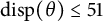 $\operatorname {{\mathrm {disp}}}(\theta )\leq 51$
, and hence the result. Consider the diagram
 $\mathsf {E}_{7;4}$
. Then,
 $\varphi _1=\varphi _{\mathsf {E}_7}$
,
 $\varphi _2=\varphi _{\mathsf {D}_6}$
,
 $\varphi _3=\varphi _{\mathsf {D}_4}$
, and
 $\varphi _4=\alpha _3$
. Replace
 $\theta $
by the conjugate
 $\theta ^{\prime }=s_1^{-1}\theta s_1$
. Because
 $s_1\varphi _1, s_1\varphi _2, s_1\varphi _3,s_1\varphi _4\geq \alpha _1$
, Lemma 4.4 gives
 $\operatorname {{\mathrm {disp}}}(\theta )=\operatorname {{\mathrm {disp}}}(\theta ^{\prime })\leq 60$
, and again the result follows.
The case
 $\Phi =\mathsf {E}_8$
: Consider the diagram
 $\mathsf {E}_{8;2}$
. Then,
 $\varphi _1=\varphi _{\mathsf {E}_8}$
and
 $\varphi _2=\varphi _{\mathsf {D}_6}$
. We claim that
 $\operatorname {{\mathrm {disp}}}(\theta )\leq 90$
. To see this, let
 $\beta =(00111111)$
be the highest root of an
 $\mathsf {A}_6$
subsystem. Then,
 $s_{\beta }\varphi _1=(23354321)$
and
 $s_{\beta }\varphi _2=(22454321)$
are the two roots of
 $\mathsf {E}_8$
with height
 $23$
. Thus, the conjugate
 $\theta ^{\prime }=s_{\beta }^{-1}\theta s_{\beta }$
satisfies
 $\theta ^{\prime }\in \langle U_{\alpha }\mid \operatorname {{\mathrm {ht}}}(\alpha )\geq 23\rangle $
, and so by Lemma 4.4 we have
 $\operatorname {{\mathrm {disp}}}(\theta )=\operatorname {{\mathrm {disp}}}(\theta ^{\prime })\leq 90$
.
Consider the diagram
 $\mathsf {E}_{8;4}$
. Then,
 $\varphi _1=\varphi _{\mathsf {E}_8}$
,
 $\varphi _2=\varphi _{\mathsf {E}_7}$
,
 $\varphi _3=\varphi _{\mathsf {D}_6}$
, and
 $\varphi _4=\alpha _7$
. By direct calculation, the roots
 $s_8\varphi _1$
,
 $s_8\varphi _2$
,
 $s_8\varphi _3$
, and
 $s_8\alpha _7$
are all elements of
 $\Phi ^+\backslash \Phi _{\mathsf {E}_7}$
. Therefore, the conjugate
 $\theta ^{\prime }=s_8^{-1}\theta s_8$
satisfies
 $\theta ^{\prime }\in \langle U_{\alpha }\mid \alpha \geq \alpha _8\rangle $
, and so by Lemma 4.4 we have
 $\operatorname {{\mathrm {disp}}}(\theta )=\operatorname {{\mathrm {disp}}}(\theta ^{\prime })\leq 108$
, completing the proof for
 $\mathsf {E}_8$
.
The case
 $\Phi =\mathsf {F}_4$
: Consider the diagram
 $\mathsf {F}_{4;2}$
. Then,
 $\varphi _1=\varphi _{\mathsf {F}_4}$
and
 $\varphi _2=\varphi _{\mathsf {C}_3}$
. Let
 $v=s_1s_2s_1$
. Then,
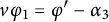 $v\varphi _1=\varphi ^{\prime }-\alpha _3$
and
 $v\varphi _2=\varphi ^{\prime }+\alpha _3$
, where
 $\varphi ^{\prime }=(1232)$
is the highest short root. Replace
 $\theta $
by the conjugate
 $\theta ^{\prime }=v\theta v^{-1}=x_{\varphi ^{\prime }-\alpha _3}(a)x_{\varphi ^{\prime }+\alpha _3}(b)$
. Let
 $X\,{=}\,\{(0100),(0010),(1100),(0120),(1120)\}$
. Then,
 $x_{\gamma }(c)\theta ^{\prime }=\theta ^{\prime } x_{\gamma }(c)$
for all
 $\gamma \in \Phi ^+\backslash X$
. Each
 $u\in U^+$
can be written as
 $u=u_1u_2$
with
 $u_1\in U_{\Phi ^+\backslash X}^+$
and
 $u_2\in U_X^+$
. Write
 $$ \begin{align*}u_2=x_{(0010)}(z_1)x_{(0120)}(z_2)x_{(1120)}(z_3)x_{(0100)}(z_4)x_{(1100)}(z_5).\end{align*} $$
Because
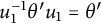 $u_1^{-1}\theta ^{\prime } u_1=\theta ^{\prime }$
, a calculation using commutator relations gives
 $$ \begin{align*} u^{-1}\theta^{\prime} u&=x_{(1222)}(a)x_{(1232)}(-z_1a)x_{(1242)}(c)x_{(1342)}(-z_4c+z_2a)x_{(2342)}(-z_5c+z_3a), \end{align*} $$
where
 $c=z_1^2a+b$
, and hence
 $$ \begin{align*} &w_0^{-1}u^{-1}\theta^{\prime} uw_0\\ &=x_{-(1222)}(-a)x_{-(1232)}(z_1a)x_{-(1242)}(-c)x_{-(1342)}(z_4c-z_2a)x_{-(2342)}(z_5c-z_3a). \end{align*} $$
Using the folding and commutator relations, we obtain that
 $Bw_0^{-1}u^{-1}\theta uw_0B$
equals
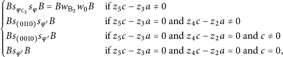 $$ \begin{align*} \begin{cases} Bs_{\varphi_{\mathsf{C}_3}}s_{\varphi}B=Bw_{\mathsf{B}_2}w_0B&\text{if}\ z_5c-z_3a\neq 0\\ Bs_{(0110)}s_{\varphi^{\prime}}B&\text{if}\ z_5c-z_3a=0\ \text{and}\ z_4c-z_2a\neq 0\\ Bs_{(0010)}s_{\varphi^{\prime}}B&\text{if}\ z_5c-z_3a=0\ \text{and}\ z_4c-z_2a= 0\ \text{and}\ c\neq 0\\ Bs_{\varphi^{\prime}}B&\text{if}\ z_5c-z_3a=0\ \text{and}\ z_4c-z_2a= 0\ \text{and}\ c=0, \end{cases} \end{align*} $$
and so by the standard technique,
 $\theta $
is domestic with opposition diagram
 $\mathsf {F}_{4;2}$
.
Finally, in special characteristic, in type
 $\mathsf {F}_4$
, the element
 $x_{\varphi ^{\prime }}(a)$
(
 $a\neq 0$
) has opposition diagram
 $\mathsf {F}_{4;4}^1$
, and in type
 $\mathsf {G}_2$
, the element
 $x_{\varphi ^{\prime }}(a)$
(
 $a\neq 0$
) has opposition diagram
 $\mathsf {G}_{2;1}^1$
(by Theorem 3.10). Moreover, very similar calculations to those above show that in type
 $\mathsf {F}_4$
, for all fields,
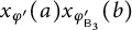 $x_{\varphi ^{\prime }}(a)x_{\varphi _{\mathsf {B}_3}^{\prime }}(b)$
with
 $a,b\neq 0$
has opposition diagram
 $\mathsf {F}_{4;2}$
, completing the proof.▪
5 Classification of domestic homologies
In this section, we classify the domestic homologies of split buildings of exceptional types. Throughout this section, we may assume that
 $\Delta $
is a large building; for over the field
 $\mathbb {F}_2$
, there are no nontrivial homologies. In Lemma 5.1, we recall the basic fact that the fixed element structure of a homology
 $\theta $
is a (typically nonthick) building
 $\Delta _{\theta }$
of the same type as
 $\Delta $
. Following Scharlau [Reference Scharlau20], the thick frame
 $\Delta _{\theta }^{\prime }$
of
 $\Delta _{\theta }$
is a thick building naturally associated to
 $\Delta _{\theta }$
, and the type
 $W_{\theta }$
of this building is a reflection subgroup of W (see below for some further details). Our classification of domestic homologies is in terms of these reflection subgroups. The data provided in Appendix A are useful for this section.
If P is a panel of
 $\Delta $
, we write
 $\mathcal {C}(P)$
for the set of chambers containing P. The proof of the following lemma is straightforward.
Lemma 5.1 Let
 $\Delta $
be a split spherical building of type
 $(W,S)$
, and let
 $\theta $
be a homology of
 $\Delta $
. Let
 $\Delta _{\theta }$
be the set of fixed chambers of
 $\theta $
. Then,
 $\Delta _{\theta }$
is a (typically nonthick) building of type
 $(W,S)$
. Moreover, if P is an s-panel of
 $\Delta $
with
 $\mathcal {C}(P)\cap \Delta _{\theta }\neq \emptyset $
, then either
 $\mathcal {C}(P)\subseteq \Delta _{\theta }$
or
 $|\mathcal {C}(P)\cap \Delta _{\theta }|=2$
.
If
 $\Delta _{\theta }$
is the fixed subbuilding of a homology
 $\theta $
, we refer to the thick (if
 $\mathcal {C}(P)\subseteq \Delta _{\theta }$
) and thin (if
 $|\mathcal {C}(P)\cap \Delta _{\theta }|=2$
) panels of
 $\Delta _{\theta }$
. If
 $\mathcal {A}$
is an apartment of
 $\Delta _{\theta }$
, then we refer to the thin and thick walls of
 $\mathcal {A}$
.
The thick frame
 $\Delta _{\theta }^{\prime }$
of
 $\Delta _{\theta }$
is a building whose chambers are the thin-classes of chambers of
 $\Delta _{\theta }$
, with adjacency given by adjacency of representatives of these classes in
 $\Delta _{\theta }$
(see [Reference Scharlau20]; here, thin-classes are the classes of the finest equivalence relation containing the thin panels). The building
 $\Delta _{\theta }^{\prime }$
has type
 $W_{\theta }$
, where
 $W_{\theta }$
is the reflection subgroup of W generated by the reflections about the thick walls of any apartment of
 $\Delta _{\theta }$
.
The embedding
 $W_{\theta }\hookrightarrow W$
is only defined up to conjugacy; however, in practice, if
 $\theta \in H$
, we fix this embedding by taking reflections in the base apartment. If
 $\theta \in H$
, then the thick walls of the base apartment
 $\mathcal {A}_0$
are easily computed as follows. Writing
 $\theta =h_{\omega _1}(c_1)\cdots h_{\omega _N}(c_N)$
, we have
 $$ \begin{align*}\theta x_{\alpha}(a)\theta^{-1}=x_{\alpha}(ac_1^{\langle\alpha,\omega_1\rangle}\cdots c_N^{\langle\alpha,\omega_N\rangle}), \end{align*} $$
and so the
 $\alpha $
-wall of the base apartment is thick if and only if
 $$ \begin{align*}c_1^{\langle\alpha,\omega_1\rangle}\cdots c_N^{\langle\alpha,\omega_N\rangle}=1.\end{align*} $$
For homologies
 $\theta \in H$
, we define the root system of
 $\theta $
by
 $$ \begin{align*}\Phi_{\theta}=\{\alpha\in\Phi\mid \theta x_{\alpha}(1)\theta^{-1}=x_{\alpha}(1)\}=\{\alpha\in \Phi\mid \text{ the}\ \alpha\text{-wall of}\ \mathcal{A}_0\ \text{is thick}\}. \end{align*} $$
It is easy to check that
 $\Phi _{\theta }$
is indeed a crystallographic root system, and note that
 $W_{\theta }$
is generated by the reflections in the hyperplanes perpendicular to the roots in
 $\Phi _{\theta }$
.
Example 5.2 Consider the homology
 $\theta =h_{\omega _5}(c)h_{\omega _6}(c^{-2})$
with
 $c^2\neq 1$
of an
 $\mathsf {E}_6$
building. Then,
 $\alpha \in \Phi _{\theta }$
if and only if
 $c^{\langle \alpha ,\omega _5\rangle -2\langle \alpha ,\omega _6\rangle }=1$
, and because
 $c^2\neq 1$
, inspection of the root system shows that
 $\Phi _{\theta }^+$
consists precisely the roots of the form
 $(****00)$
(there are
 $10$
such roots) or
 $(****21)$
(there are five such roots). Hence,
 $|\Phi _{\theta }^+|=15$
. Scharlau’s classification [Reference Scharlau20, Proposition 2] (see below) forces
 $\Delta _{\theta }^{\prime }$
to have type
 $\mathsf {A}_5$
, lying inside of a maximal reflection subgroup of type
 $\mathsf {A}_5\times \mathsf {A}_1$
. To see this, note that
 $\mathsf {A}_2\times \mathsf {A}_2\times \mathsf {A}_2$
has only nine reflections, eliminating this case. Then,
 $\mathsf {D}_5$
has
 $20$
reflections; however, the maximal reflection subgroups of
 $\mathsf {D}_5$
have types
 $\mathsf {D}_3\times \mathsf {D}_2$
(
 $6+2=8$
reflections),
 $\mathsf {D}_4$
(
 $12$
reflections), or
 $\mathsf {A}_4$
(
 $10$
reflections), eliminating these possibilities.
Let us now outline our strategy for classifying domestic homologies. Let
 $\theta $
be a homology, and after conjugating, we assume that
 $\theta \in H$
, and so the base apartment
 $\mathcal {A}_0$
of
 $\Delta $
is fixed by
 $\theta $
. Let
 $W_{\theta }$
be the reflection subgroup of W generated by the thick walls of
 $\mathcal {A}_0$
. This subgroup in turn lies in a maximal reflection subgroup
 $W_{\theta }^{\prime }$
of W. By [Reference Scharlau20, Proposition 2], each maximal reflection subgroup is determined up to conjugation by its type, and hence we may assume the root system of
 $W_{\theta }^{\prime }$
has simple roots as listed below for the cases that we will require (where
 $\mathsf {D}_2=\mathsf {A}_1\times \mathsf {A}_1$
, and
 $\mathsf {D}_3=\mathsf {A}_3$
in the natural way):
-
(1) The maximal reflection subgroups of
$\mathsf {B}_4$
are:-
(a)
$\mathsf {B}_3\times \mathsf {A}_1$
, with simple roots
$(\alpha _2,\alpha _3,\alpha _4)\times (\alpha _1+\alpha _2+\alpha _3+\alpha _4)$
. -
(b)
$\mathsf {B}_2\times \mathsf {B}_2$
, with simple roots
$(\alpha _3,\alpha _4)\times (\alpha _1,\alpha _2+\alpha _3+\alpha _4)$
. -
(c)
$\mathsf {D}_4$
, with simple roots
$(\alpha _1,\alpha _2,\alpha _3,\alpha _3+2\alpha _4)$
.
-
-
(2) The maximal reflection subgroups of
$\mathsf {F}_4$
are:-
(a)
$\mathsf {B}_4$
, with simple roots
$(\varphi _{\mathsf {C}_3},\alpha _1,\alpha _2,\alpha _3)$
where
$\varphi _{\mathsf {C}_3}=\alpha _2+2\alpha _3+2\alpha _4$
. -
(b)
$\mathsf {C}_3\times \mathsf {A}_1$
, with simple roots
$(\alpha _4,\alpha _3,\alpha _2)\times (\varphi )$
. -
(c)
$\mathsf {A}_2\times \mathsf {A}_2$
, with simple roots
$(\alpha _3,\alpha _4)\times (\alpha _1,\varphi -\alpha _1)$
.
-
-
(3) The maximal reflection subgroups of
$\mathsf {D}_5$
are:-
(a)
$\mathsf {D}_3\times \mathsf {D}_2$
, with simple roots
$(\alpha _3,\alpha _4,\alpha _5)\times (\alpha _1,\varphi )$
. -
(b)
$\mathsf {D}_4$
, with simple roots
$(\alpha _2,\alpha _3,\alpha _4,\alpha _5)$
. -
(c)
$\mathsf {A}_4$
, with simple roots
$(\alpha _1,\alpha _2,\alpha _3,\alpha _4)$
.
-
-
(4) The maximal reflection subgroups of
$\mathsf {D}_6$
are:-
(a)
$\mathsf {D}_4\times \mathsf {D}_2$
, with simple roots
$(\alpha _3,\alpha _4,\alpha _5,\alpha _6)\times (\alpha _1,\varphi )$
. -
(b)
$\mathsf {D}_3\times \mathsf {D}_3$
, with simple roots
$(\alpha _4,\alpha _5,\alpha _6)\times (\alpha _1,\alpha _2,\varphi -\alpha _1-\alpha _2)$
. -
(c)
$\mathsf {D}_5$
, with simple roots
$(\alpha _2,\alpha _3,\alpha _4,\alpha _5,\alpha _6)$
. -
(d)
$\mathsf {A}_5$
, with simple roots
$(\alpha _1,\alpha _2,\alpha _3,\alpha _4,\alpha _5)$
.
-
-
(5) The maximal reflection subgroups of
$\mathsf {E}_6$
are:-
(a)
$\mathsf {A}_5\times \mathsf {A}_1$
, with simple roots
$(\alpha _1,\alpha _3,\alpha _4,\alpha _5,\alpha _6)\times (\varphi )$
. -
(b)
$\mathsf {A}_2\times \mathsf {A}_2\times \mathsf {A}_2$
, with simple roots
$(\alpha _1,\alpha _3)\times (\alpha _5,\alpha _6)\times (\alpha _2,\varphi -\alpha _2)$
. -
(c)
$\mathsf {D}_5$
, with simple roots
$(\alpha _1,\alpha _3,\alpha _4,\alpha _2,\alpha _5)$
.
-
-
(6) The maximal reflection subgroups of
$\mathsf {E}_7$
are:-
(a)
$\mathsf {A}_7$
, with simple roots
$(\alpha _1,\alpha _3,\alpha _4,\alpha _5,\alpha _6,\alpha _7,\varphi _{\mathsf {E}_6})$
. -
(b)
$\mathsf {D}_6\times \mathsf {A}_1$
, with simple roots
$(\alpha _7,\alpha _6,\alpha _5,\alpha _4,\alpha _2,\alpha _3)\times (\varphi )$
. -
(c)
$\mathsf {A}_5\times \mathsf {A}_2$
, with simple roots
$(\alpha _2,\alpha _4,\alpha _5,\alpha _6,\alpha _7)\times (\alpha _1,\varphi -\alpha _1)$
. -
(d)
$\mathsf {E}_6$
, with simple roots
$(\alpha _1,\alpha _2,\alpha _3,\alpha _4,\alpha _5,\alpha _6)$
.
-
-
(7) The maximal reflection subgroups of
$\mathsf {E}_8$
are:-
(a)
$\mathsf {D}_8$
, with simple roots
$(\varphi _{\mathsf {E}_7},\alpha _8,\alpha _7,\alpha _6,\alpha _5,\alpha _4,\alpha _2,\alpha _3)$
. -
(b)
$\mathsf {A}_8$
, with simple roots
$(\varphi -\varphi _{\mathsf {A}_7},\alpha _1,\alpha _3,\alpha _4,\alpha _5,\alpha _6,\alpha _7,\alpha _8)$
. -
(c)
$\mathsf {A}_4\times \mathsf {A}_4$
, with simple roots
$(\alpha _1,\alpha _3,\alpha _4,\alpha _2)\times (\varphi -\alpha _6-\alpha _7-\alpha _8,\alpha _6,\alpha _7,\alpha _8)$
. -
(d)
$\mathsf {E}_6\times \mathsf {A}_2$
, with simple roots
$(\alpha _1,\alpha _2,\alpha _3,\alpha _4,\alpha _5,\alpha _6)\times (\alpha _8,\varphi -\alpha _8)$
. -
(e)
$\mathsf {E}_7\times \mathsf {A}_1$
, with simple roots
$(\alpha _1,\alpha _2,\alpha _3,\alpha _4,\alpha _5,\alpha _6,\alpha _7)\times (\varphi )$
.
-


























































In cases (2)–(7), the root system of the reflection subgroup is simply the intersection of the
 $\mathbb {Z}$
-span of the simple roots with the ambient root system. In case (1), the intersection of the
 $\mathbb {Z}$
-span of the simple roots with the ambient root system is larger than the stated type, and thus one must restrict coefficients in the linear combinations appropriately to obtain the correct type.
Our strategy is as follows.
-
(A) We first identify a list of reflection subgroups
$W^{\prime }$
of W such that every homology with
$W_{\theta }=W^{\prime }$
is domestic (we will then call
$W^{\prime }$
domestic). -
(B) We then show that if
$W^{\prime }$
is a reflection subgroup of W not in our list from (A), then every homology with
$W_{\theta }=W^{\prime }$
is not domestic (we will then call
$W^{\prime }$
nondomestic).


We prove (A) using the standard technique (Proposition 2.8), with some more refined arguments required in the
 $\mathsf {E}_7$
and
 $\mathsf {F}_4$
cases. Our strategy for proving (B) is via the following lemma.
Lemma 5.3 Let
 $\theta \in H$
be a homology with root system
 $\Phi _{\theta }$
. Suppose there exist mutually perpendicular roots
 $\beta _1,\ldots ,\beta _k\in \Phi ^+\backslash \Phi _{\theta }$
. Then,
 $$ \begin{align*}\operatorname{{\mathrm{disp}}}(\theta)\geq M,\quad\text{where}\ M=\ell(s_{\beta_1}\cdots s_{\beta_k}). \end{align*} $$
Moreover, if
 $\theta ^{\prime }\in H$
is a homology with root system
 $\Phi _{\theta ^{\prime }}\subseteq \Phi _{\theta }$
, then
 $\operatorname {{\mathrm {disp}}}(\theta ^{\prime })\geq M$
.
Proof Consider the chamber
 $gB=uw_0B$
with
 $u=x_{\beta _1}(1)\cdots x_{\beta _k}(1)$
. Because
 $\beta _1,\ldots ,\beta _k\notin \Phi _{\theta }$
, we have
 $\theta u\theta ^{-1}=x_{\beta _1}(c_1)\cdots x_{\beta _k}(c_k)$
with
 $c_1,\ldots ,c_k\neq 1$
. Moreover, the elements
 $x_{\beta _1}(a_1),\ldots ,x_{\beta _k}(a_k)$
, with
 $a_1,\ldots ,a_k\in \mathbb {F}$
, commute with each other (as the roots are mutually perpendicular), and hence
 $$ \begin{align*}Bg^{-1}\theta gB=Bw_0^{-1}u^{-1}\theta uw_0B=Bx_{-\beta_1}(c_1-1)\cdots x_{-\beta_k}(c_k-1)B. \end{align*} $$
Thus, by Lemma 2.1, we have
 $ Bg^{-1}\theta gB=Bs_{\beta _1}\cdots s_{\beta _k}B, $
and hence
 $\operatorname {{\mathrm {disp}}}(\theta )\geq \ell (s_{\beta _1}\cdots s_{\beta _k})$
. The final statement follows as
 $\beta _1,\ldots ,\beta _k\in \Phi ^+\backslash \Phi _{\theta }^{\prime }$
.▪
Note that if Lemma 5.3 is used to prove nondomesticity for a homology
 $\theta $
(by finding mutually perpendicular roots
 $\beta _1,\ldots ,\beta _k\in \Phi ^+\backslash \Phi _{\theta }$
with
 $\ell (s_{\beta _1}\cdots s_{\beta _k})$
sufficiently large), then every homology
 $\theta ^{\prime }$
with
 $W_{\theta ^{\prime }}$
a reflection subgroup of
 $W_{\theta }$
is also nondomestic, as
 $\Phi _{\theta ^{\prime }}\subseteq \Phi _{\theta }$
. Thus, to prove (B), it suffices to prove nondomesticity for the maximal reflection subgroups in the poset of reflection subgroups of W excluding those in the list from (A).
We now proceed with our classification of domestic homologies of split exceptional buildings.
Theorem 5.4 A nontrivial homology
 $\theta $
of
 $\mathsf {E}_6(\mathbb {F})$
is domestic if and only if
 $\Delta _{\theta }^{\prime }$
is of type
 $\mathsf {D}_5$
. Moreover, all such homologies have opposition diagram
 ${^2}\mathsf {E}_{6;2}$
, and are conjugate to an element of the form
 $h_{\omega _6}(c)$
with
 $c\in \mathbb {F}\backslash \{0,1\}$
.
Proof Let
 $\theta \in H$
. Suppose that
 $\Delta _{\theta }^{\prime }$
is of type
 $\mathsf {D}_5$
. After conjugation, we may assume that
 $\Phi _{\theta }$
has simple roots
 $(\alpha _1,\alpha _3,\alpha _4,\alpha _2,\alpha _5)$
. The condition
 $\theta x_{\alpha }(a)\theta ^{-1}=x_{\alpha }(a)$
for these simple roots forces
 $\theta =h_{\omega _6}(c)$
for some
 $c\neq 1$
. We show that
 $\theta $
is domestic, with diagram
 ${^2}\mathsf {E}_{6;2}$
. Let
 $\Phi _6^+=\{\alpha \in \Phi ^+\mid \langle \alpha ,\omega _6\rangle =1\}$
, and let
 $w_1=w_0w_{\mathsf {D}_5}$
. Let
 $u\in U^+$
, and write
 $u=u_1u_2$
with
 $u_1\in U_{\mathsf {D}_5}^+$
and
 $u_2\in U_{\Phi _6}^+$
. Because
 $u_1^{-1}\theta u_1=\theta $
and
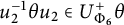 $u_2^{-1}\theta u_2\in U_{\Phi _6}^+\theta $
, we have
 $$ \begin{align*} w_1^{-1}w_0^{-1}u^{-1}\theta uw_0w_1&=w_{\mathsf{D}_5}^{-1}u_2^{-1}\theta u_2w_{\mathsf{D}_5}\in w_{\mathsf{D}_5}^{-1}U_{\Phi_6}^+w_{\mathsf{D}_5}\theta\subseteq B, \end{align*} $$
where we have used the fact that
 $\Phi (w_{\mathsf {D}_5})=\Phi ^+\backslash \Phi _6$
. Because
 $\ell (w_1)=36-20=16$
, the standard technique (Proposition 2.8) gives
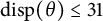 $\operatorname {{\mathrm {disp}}}(\theta )\leq 31$
. Moreover, because
 $\theta =h_{\omega _6}(c)$
is not conjugate to a root elation, it must have opposition diagram
 ${^2}\mathsf {E}_{6;2}$
(by Theorem 3.4 and the classification of admissible diagrams).
We now use Lemma 5.3 to show that if
 $\theta \in H$
is a nontrivial homology with
 $\Delta _{\theta }^{\prime }$
not of type
 $\mathsf {D}_5$
, then
 $\theta $
is not domestic. As noted above, it is sufficient to consider the maximal elements in the poset of reflection subgroups of W excluding those of type
 $\mathsf {D}_5$
. Thus, we may assume that
 $W_{\theta }$
is either a maximal reflection subgroup of W of type
 $\mathsf {A}_5\times \mathsf {A}_1$
or
 $\mathsf {A}_2\times \mathsf {A}_2\times \mathsf {A}_2$
, or a maximal reflection subgroup of the standard
 $\mathsf {D}_5$
subgroup of W. Up to conjugation, we may suppose that either:
-
(1)
$\Phi _{\theta }=\mathsf {A}_5\times \mathsf {A}_1$
with simple roots
$(\alpha _1,\alpha _3,\alpha _4,\alpha _5,\alpha _6)\times (\varphi )$
. The
$16$
positive roots of
$\Phi $
are precisely the roots
$\alpha \in \Phi ^+$
with
$\langle \alpha ,\omega _2\rangle \in 2\mathbb {Z}$
. -
(2)
$\Phi _{\theta }=\mathsf {A}_2\times \mathsf {A}_2\times \mathsf {A}_2$
with simple roots
$(\alpha _1,\alpha _3)\times (\alpha _5,\alpha _6)\times (\alpha _2,\varphi -\alpha _2)$
. The nine positive roots are precisely the roots
$\alpha \in \Phi ^+$
with
$\langle \alpha ,\omega _4\rangle \in 3\mathbb {Z}$
. -
(3)
$\Phi _{\theta }=\mathsf {D}_3\times \mathsf {D}_2$
with simple roots
$(\alpha _4,\alpha _2,\alpha _5)\times (\alpha _1,\alpha _1+\alpha _2+2\alpha _3+2\alpha _4+\alpha _5)$
. The eight positive roots are precisely the roots
$\alpha \in \Phi ^+$
with both
$\langle \alpha ,\omega _3\rangle \in 2\mathbb {Z}$
and
$\langle \alpha ,\omega _6\rangle =0$
. -
(4)
$\Phi _{\theta }=\mathsf {D}_4$
with simple roots are
$(\alpha _3,\alpha _4,\alpha _2,\alpha _5)$
. The
$12$
positive roots are precisely the roots
$\alpha \in \Phi ^+$
with both
$\langle \alpha ,\omega _1\rangle =0$
and
$\langle \alpha ,\omega _6\rangle =0$
. -
(5)
$\Phi _{\theta }=\mathsf {A}_4$
with simple roots are
$(\alpha _1,\alpha _3,\alpha _4,\alpha _2)$
. The
$10$
positive roots are precisely the roots
$\alpha \in \Phi ^+$
with both
$\langle \alpha ,\omega _5\rangle =0$
and
$\langle \alpha ,\omega _6\rangle =0$
.




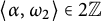



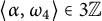



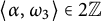








In cases (1), (2), (3), and (5), we have
 $\alpha ,\beta ,\gamma \in \Phi ^+\backslash \Phi _{\theta }$
, where
 $\alpha ,\beta ,\gamma $
are the mutually perpendicular roots
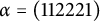 $\alpha =(112221)$
,
 $\beta =(111211)$
, and
 $\gamma =(011210)$
. Thus, by Lemma 5.3, we have
 $\operatorname {{\mathrm {disp}}}(\theta )\geq \ell (s_{\alpha }s_{\beta }s_{\gamma })$
. Moreover, note that the roots
 $\alpha $
,
 $\beta $
,
 $\gamma $
,
 $\alpha _2$
are mutually perpendicular and invariant under the diagram automorphism of
 $\mathsf {E}_6$
, and so by Lemma 2.3 we have
 $s_{\alpha }s_{\beta }s_{\gamma }s_2=w_0$
. Thus,
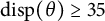 $\operatorname {{\mathrm {disp}}}(\theta )\geq 35$
, and so
 $\theta $
is not domestic.
In case (4), we have
 $\alpha ^{\prime },\beta ^{\prime },\gamma ^{\prime }\in \Phi ^+\backslash \Phi _{\theta }$
, where
 $\alpha ^{\prime },\beta ^{\prime },\gamma ^{\prime }$
are the mutually perpendicular roots
 $\alpha ^{\prime }=\varphi $
,
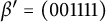 $\beta ^{\prime }=(001111)$
, and
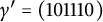 $\gamma ^{\prime }=(101110)$
. Thus,
 $\operatorname {{\mathrm {disp}}}(\theta )\geq \ell (w)$
, where
 $w=s_{\alpha ^{\prime }}s_{\beta ^{\prime }}s_{\gamma ^{\prime }}$
. It is easy to see that
 $\Phi (w)=\Phi ^+\backslash \{\alpha _1,\alpha _4,\alpha _6\}$
, and hence
 $\ell (w)=33$
. It follows that
 $\theta $
is not domestic.▪
Lemma 5.5 Let
 $c\in \mathbb {F}\backslash \{0,1\}$
. The homology
 $\theta =h_{\omega _1}(c)$
of
 $\mathsf {E}_7(\mathbb {F})$
is domestic, with opposition diagram
 $\mathsf {E}_{7;4}$
.
Proof We first prove directly that
 $\theta $
is
 $\{7\}$
-domestic. Consider the
 $\mathsf {E}_{7,7}(\mathbb {F})$
geometry, with point set
 $G/P_7$
. By Corollary 2.7, it is sufficient to show that no point opposite the base point
 $P_7$
in this geometry is mapped onto an opposite point by
 $\theta $
. The points opposite
 $P_7$
are of the form
 $uyP_7$
, where
 $y=w_{\mathsf {E}_7}w_{\mathsf {E}_6}$
, and
 $u\in U_{\Phi (y)}^+$
. We are required to show that
 $$ \begin{align*}P_7y^{-1}u^{-1}\theta uyP_7\neq P_7yP_7\quad\text{for all}\ u\in U_{\Phi(y)}^+. \end{align*} $$
Let
 $\Phi _{1}$
be the subsystem with simple roots
 $(\alpha _7,\alpha _6,\alpha _5,\alpha _4,\alpha _2,\alpha _3)$
. Then,
 $\Phi _{1}\subseteq \Phi _{\theta }$
(equality occurs if
 $c\neq -1$
, while if
 $c=-1$
, then
 $\Phi _{\theta }=\Phi _{1}\cup \{\pm \varphi \}$
). In particular,
 $\theta x_{\alpha }(a)\theta ^{-1}=x_{\alpha }(a)$
for all
 $\alpha \in \Phi _{1}$
. Write
 $u=u_1u_2$
with
 $u_1\in U_{\Phi _{1}}^+$
and
 $u_2\in U_{\Phi \backslash \Phi _{1}}^+$
. Then,
 $$ \begin{align*}P_7y^{-1}u^{-1}\theta uyP_7=P_7y^{-1}u_2^{-1}\theta u_2yP_7. \end{align*} $$
By the commutator relations, we have
 $u_3=u_2^{-1}\theta u_2\theta ^{-1}\in U_{\Phi \backslash \Phi _1}^+$
, and because
 $yP_7=w_0P_7$
, we have
 $$ \begin{align*}P_7y^{-1}u^{-1}\theta uyP_7=P_7w_0^{-1}u_3w_0P_7=P_7\tilde{u}P_7, \end{align*} $$
where
 $\tilde {u}\in U_{\Phi \backslash \Phi _1}^-$
. Because
 $\Phi (s_{\varphi })=\Phi ^+\backslash \Phi _1^+$
, we have
 $$ \begin{align} P_7y^{-1}u^{-1}\theta uyP_7=P_7s_{\varphi}(s_{\varphi}^{-1}\tilde{u}s_{\varphi})s_{\varphi}^{-1}P_7\subseteq P_7s_{\varphi}P_7\cdot P_7s_{\varphi}P_7. \end{align} $$
It follows from Lemma 4.2 that
 $P_7s_{\varphi }P_7\cdot P_7s_{\varphi }P_7\cap P_7yP_7=\emptyset $
. Thus, we have shown that
 $\theta $
is
 $\{7\}$
-domestic, and hence domestic. Because
 $\theta $
is neither a root elation nor a product of perpendicular root elations, it does not have opposition diagram
 $\mathsf {E}_{7;1}$
or
 $\mathsf {E}_{7;2}$
, and because
 $\theta $
is
 $\{7\}$
-domestic, it does not have opposition diagram
 $\mathsf {E}_{7;3}$
. Thus,
 $\theta $
has opposition diagram
 $\mathsf {E}_{7;4}$
.▪
Theorem 5.6 A nontrivial homology
 $\theta $
of
 $\mathsf {E}_7(\mathbb {F})$
is domestic if and only if
 $\Delta _{\theta }^{\prime }$
is of type:
-
(1)
$\mathsf {E}_6$
, in which case
$\theta $
has opposition diagram
$\mathsf {E}_{7;3}$
and is conjugate to an element of the form
$h_{\omega _7}(c)$
with
$c\in \mathbb {F}\backslash \{0,1\}$
; -
(2)
$\mathsf {D}_6$
, in which case
$\theta $
has opposition diagram
$\mathsf {E}_{7;4}$
and is conjugate to an element of the form
$h_{\omega _1}(c)$
with
$c\in \mathbb {F}\backslash \{0,1,-1\}$
; -
(3)
$\mathsf {D}_6\times \mathsf {A}_1$
, in which case
$\mathrm {char}(\mathbb {F})\neq 2$
and
$\theta $
has opposition diagram
$\mathsf {E}_{7;4}$
and is conjugate to
$h_{\omega _1}(-1)$
.





Proof We begin by showing that if
 $\Delta _{\theta }^{\prime }$
has type
 $\mathsf {E}_6$
,
 $\mathsf {D}_6$
, or
 $\mathsf {D}_6\times \mathsf {A}_1$
, then
 $\theta $
is domestic, with the stated diagram and conjugacy class.
Suppose that
 $\Phi _{\theta }$
is of type
 $\mathsf {E}_6$
. The
 $36$
positive roots of this system are precisely those
 $\alpha \in \Phi ^+$
with
 $\langle \alpha ,\omega _7\rangle =0$
, and thus
 $\theta =h_{\omega _7}(c)$
for some
 $c\neq 1$
. Let
 $\Phi _7^+=\{\alpha \in \Phi ^+\mid \langle \alpha ,\omega _7\rangle =1\}$
, and note that
 $\Phi ^+=\Phi _{\theta }\sqcup \Phi _7^+$
. Arguing as in the
 $\mathsf {E}_6$
case (Theorem 5.4), and using the standard technique with
 $w_1=w_0w_{\mathsf {E}_6}$
, we see that
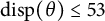 $\operatorname {{\mathrm {disp}}}(\theta )\leq 53$
(as
 $\ell (w_1)=27$
). Because
 $\theta $
is neither conjugate to a root elation nor to a product of two perpendicular root elations, it does not have opposition diagram
 $\mathsf {E}_{7;1}$
or
 $\mathsf {E}_{7;2}$
, and because
 $\operatorname {{\mathrm {disp}}}(\theta )<60$
, it does not have opposition diagram
 $\mathsf {E}_{7;4}$
. Thus, it follows from the classification of opposition diagrams that
 $\theta $
has diagram
 $\mathsf {E}_{7;3}$
.
Now, suppose that
 $\Phi _{\theta }$
is of type
 $\mathsf {D}_6$
or
 $\mathsf {D}_6\times \mathsf {A}_1$
. The positive roots of
 $\Phi _{\theta }$
are
 $$ \begin{align*} \Phi_{\mathsf{D}_6}^+=\{\alpha\in\Phi^+\mid \langle\alpha,\omega_1\rangle=0\},\quad \Phi_{\mathsf{D}_6\times\mathsf{A}_1}^+=\{\alpha\in\Phi^+\mid \langle\alpha,\omega_1\rangle\in 2\mathbb{Z}\}=\Phi_{\mathsf{D}_6}^+\cup\{\varphi\}. \end{align*} $$
In particular,
 $\theta =h_{\omega _1}(c)$
where
 $c\in \mathbb {F}\backslash \{0,1,-1\}$
in the
 $\mathsf {D}_6$
case, and
 $c=-1$
in the
 $\mathsf {D}_6\times \mathsf {A}_1$
case. Thus, by Lemma 5.5,
 $\theta $
is domestic with opposition diagram
 $\mathsf {E}_{7;4}$
(note that the standard technique does not apply in this case, as
 $\ell (w_0w_{\mathsf {D}_6})=33>\ell (w_0)/2$
).
We now use Lemma 5.3 to show that if
 $\theta \in H$
is a nontrivial homology with
 $\Delta _{\theta }^{\prime }$
not of type
 $\mathsf {E}_6$
,
 $\mathsf {D}_6$
, or
 $\mathsf {D}_6\times \mathsf {A}_1$
, then
 $\theta $
is not domestic. It is sufficient to consider the maximal elements in the poset of reflection subgroups of W excluding those of types
 $\mathsf {E}_6$
,
 $\mathsf {D}_6$
, and
 $\mathsf {D}_6\times \mathsf {A}_1$
. Thus, we may assume that
 $W_{\theta }$
is either a maximal reflection subgroup of W of type
 $\mathsf {A}_7$
or
 $\mathsf {A}_5\times \mathsf {A}_2$
, or a maximal reflection subgroup of the standard
 $\mathsf {D}_6\times \mathsf {A}_1$
of
 $\mathsf {E}_6$
subgroups of W (excluding the domestic
 $\mathsf {D}_6$
subgroup). Thus, using the explicit choices of simple roots listed earlier, we may suppose that either:
-
(1)
$\Phi _{\theta }=\mathsf {A}_7$
, with
$\Phi _{\theta }^+=\{\alpha \in \Phi ^+\mid \langle \alpha ,\omega _2\rangle \in 2\mathbb {Z}\}$
. -
(2)
$\Phi _{\theta }=\mathsf {A}_5\times \mathsf {A}_2$
, with
$\Phi _{\theta }^+=\{\alpha \in \Phi ^+\mid \langle \alpha ,\omega _3\rangle \in 3\mathbb {Z}\}$
. -
(3)
$\Phi _{\theta }=(\mathsf {D}_4\times \mathsf {D}_2)\times \mathsf {A}_1$
, with
$\Phi _{\theta }^+=\{\alpha \in \Phi ^+\mid \langle \alpha ,\omega _1\rangle =0\text { and }\langle \alpha ,\omega _6\rangle \in 2\mathbb {Z}\}\cup \{\varphi \}$
. -
(4)
$\Phi _{\theta }=(\mathsf {D}_3\times \mathsf {D}_3)\times \mathsf {A}_1$
, with
$\Phi _{\theta }^+=\{\alpha \in \Phi ^+\mid \langle \alpha ,\omega _1\rangle =0\text { and }\langle \alpha ,\omega _5\rangle \in 2\mathbb {Z}\}\cup \{\varphi \}$
. -
(5)
$\Phi _{\theta }=\mathsf {D}_5\times \mathsf {A}_1$
, with
$\Phi _{\theta }^+=\{\alpha \in \Phi ^+\mid \langle \alpha ,\omega _1-2\omega _7\rangle =0\}$
. -
(6)
$\Phi _{\theta }=\mathsf {A}_5\times \mathsf {A}_1$
(contained in
$\mathsf {D}_6\times \mathsf {A}_1$
), with
$\Phi _{\theta }^+=\{\alpha \in \Phi ^+\mid 3\langle \alpha ,\omega _1\rangle =2\langle \alpha ,\omega _3\rangle \}$
. -
(7)
$\Phi _{\theta }=\mathsf {A}_5\times \mathsf {A}_1$
(contained in
$\mathsf {E}_6$
), with
$\Phi _{\theta }^+=\{\alpha \in \Phi ^+\mid \langle \alpha ,\omega _2\rangle \in 2\mathbb {Z}\text { and }\langle \alpha ,\omega _7\rangle =0\}$
. -
(8)
$\Phi _{\theta }=\mathsf {A}_2\times \mathsf {A}_2\times \mathsf {A}_2$
, with
$\Phi _{\theta }^+=\{\alpha \in \Phi ^+\mid \langle \alpha ,\omega _4\rangle \in 3\mathbb {Z}\text { and }\langle \alpha ,\omega _7\rangle =0\}$
. -
(9)
$\Phi _{\theta }=\mathsf {D}_5$
, with
$\Phi _{\theta }^+=\{\alpha \in \Phi ^+\mid \langle \alpha ,\omega _6\rangle =0\text { and }\langle \alpha ,\omega _7\rangle =0\}$
.




















In case (1), note that
 $\beta _1,\ldots ,\beta _7\notin \Phi _{\theta }$
, where
 $\beta _1=(1 1 1 1 1 0 0)$
,
 $\beta _2=(0 1 1 2 1 0 0)$
,
 $\beta _3=(0 1 1 1 1 1 0)$
,
 $\beta _4=(0 1 0 1 1 1 1)$
,
 $\beta _5=(1 1 1 2 1 1 0)$
,
 $\beta _6=(1 1 2 2 1 1 1)$
, and
 $\beta _7=(1 1 2 3 3 2 1)$
. These roots are mutually perpendicular, and so by Lemma 2.2 we have
 $s_{\beta _1}\cdots s_{\beta _7}=w_0$
. Thus, by Lemma 5.3, the homology
 $\theta $
is not domestic.
In cases (2)–(6), note that
 $\gamma _1,\ldots ,\gamma _5\notin \Phi _{\theta }$
, where
 $\gamma _1=(1 1 1 1 0 0 0)$
,
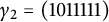 $\gamma _2=(1 0 1 1 1 1 1)$
,
 $\gamma _3=(0 1 1 2 1 1 1)$
,
 $\gamma _4=(1 1 2 3 2 1 0)$
, and
 $\gamma _5=(1 2 2 3 3 2 1)$
. The roots
 $\gamma _1,\ldots ,\gamma _5,\alpha _3,\alpha _6$
are mutually perpendicular, and so
 $s_{\gamma _1}\cdots s_{\gamma _5}=w_0s_3s_6$
. Thus,
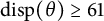 $\operatorname {{\mathrm {disp}}}(\theta )\geq 61$
, and so
 $\theta $
is not domestic.
In cases (7)–(9), note that
 $\delta _1,\ldots ,\delta _5\notin \Phi _{\theta }$
, where
 $\delta _1=(0 0 0 0 0 1 1)$
,
 $\delta _2=(0 1 0 1 1 1 0)$
,
 $\delta _3=(1 1 2 2 1 1 0)$
,
 $\delta _4=(1 2 2 3 2 1 1)$
, and
 $\delta _5=(1 1 2 3 3 2 1)$
. The roots
 $\delta _1,\ldots ,\delta _5,\alpha _1,\alpha _4$
are mutually perpendicular, and so as above
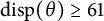 $\operatorname {{\mathrm {disp}}}(\theta )\geq 61$
and so
 $\theta $
is not domestic.▪
Theorem 5.7 A nontrivial homology
 $\theta $
of
 $\mathsf {E}_8(\mathbb {F})$
is domestic if and only if
 $\Delta _{\theta }^{\prime }$
is of type:
-
(1)
$\mathsf {E}_7$
, in which case
$\theta $
is conjugate to an element
$h_{\omega _8}(c)$
with
$c\in \mathbb {F}\backslash \{0,1,-1\}$
; -
(2)
$\mathsf {E}_7\times \mathsf {A}_1$
, in which case
$\mathrm {char}(\mathbb {F})\neq 2$
and
$\theta $
is conjugate to
$h_{\omega _8}(-1)$
.





In both cases,
 $\theta $
has opposition diagram
 $\mathsf {E}_{8;4}$
.
Proof Let
 $\theta \in H$
. Suppose that
 $\Delta _{\theta }^{\prime }$
has type
 $\mathsf {E}_7$
or
 $\mathsf {E}_7\times \mathsf {A}_1$
. After conjugating, we may suppose that
 $\Phi _{\mathsf {E}_7}\subseteq \Phi _{\theta }$
, where
 $\Phi _{\mathsf {E}_7}$
is the standard
 $\mathsf {E}_7$
subsystem of
 $\Phi $
. Thus,
 $\theta =h_{\omega _8}(c)$
for some
 $c\in \mathbb {F}\backslash \{0,1\}$
. As in the
 $\mathsf {E}_6$
case (Theorem 5.4), using the standard technique with
 $w_1=w_0w_{\mathsf {E}_7}$
, we see that
 $\operatorname {{\mathrm {disp}}}(\theta )\leq 113$
(as
 $\ell (w_1)=57$
). Because
 $\theta $
is neither conjugate to a root elation nor to a product of two perpendicular root elations, it does not have opposition diagram
 $\mathsf {E}_{8;1}$
or
 $\mathsf {E}_{8;2}$
, and hence
 $\theta $
has opposition diagram
 $\mathsf {E}_{8;4}$
.
We now use Lemma 5.3 to show that if
 $\theta \in H$
is a nontrivial homology with
 $\Delta _{\theta }^{\prime }$
not of type
 $\mathsf {E}_7$
or
 $\mathsf {E}_7\times \mathsf {A}_1$
, then
 $\theta $
is not domestic. It is sufficient to consider the maximal elements in the poset of reflection subgroups of W excluding those of types
 $\mathsf {E}_7$
and
 $\mathsf {E}_7\times \mathsf {A}_1$
. Thus, we may assume that
 $W_{\theta }$
is either a maximal reflection subgroup of W of type
 $\mathsf {D}_8$
,
 $\mathsf {A}_8$
,
 $\mathsf {A}_4\times \mathsf {A}_4$
, or
 $\mathsf {E}_6\times \mathsf {A}_2$
, or a maximal reflection subgroup of the
 $\mathsf {E}_7\times \mathsf {A}_1$
subgroup of W (excluding the domestic
 $\mathsf {E}_7$
subgroup). Thus, using the explicit choices of simple roots listed earlier, we may suppose that either:
-
(1)
$\Phi _{\theta }=\mathsf {D}_8$
, with
$\Phi _{\theta }^+=\{\alpha \in \Phi ^+\mid \langle \alpha ,\omega _1\rangle \in 2\mathbb {Z}\}$
. -
(2)
$\Phi _{\theta }=\mathsf {A}_8$
, with
$\Phi _{\theta }^+=\{\alpha \in \Phi ^+\mid \langle \alpha ,\omega _2\rangle \in 3\mathbb {Z}\}$
. -
(3)
$\Phi _{\theta }=\mathsf {A}_4\times \mathsf {A}_4$
, with
$\Phi _{\theta }^+=\{\alpha \in \Phi ^+\mid \langle \alpha ,\omega _5\rangle \in 5\mathbb {Z}\}$
. -
(4)
$\Phi _{\theta }=\mathsf {E}_6\times \mathsf {A}_2$
, with
$\Phi _{\theta }^+=\{\alpha \in \Phi ^+\mid \langle \alpha ,\omega _7\rangle \in 3\mathbb {Z}\}$
. -
(5)
$\Phi _{\theta }=\mathsf {A}_7\times \mathsf {A}_1$
, with
$\Phi _{\theta }^+=\{\alpha \in \Phi ^+\mid \langle \alpha ,\omega _2\rangle =2\langle \alpha ,\omega _7\rangle \text { and }\langle \alpha ,\omega _8\rangle =0\}\cup \{\varphi \}$
. -
(6)
$\Phi _{\theta }=(\mathsf {D}_6\times \mathsf {A}_1)\times \mathsf {A}_1$
, with
$\Phi _{\theta }^+=\{\alpha \in \Phi ^+\mid \langle \alpha ,\omega _1\rangle \in 2\mathbb {Z}\text { and }\langle \alpha ,\omega _8\rangle =0\}\cup \{\varphi \}$
. -
(7)
$\Phi _{\theta }=(\mathsf {A}_5\times \mathsf {A}_2)\times \mathsf {A}_1$
, with
$\Phi _{\theta }^+=\{\alpha \in \Phi ^+\mid \langle \alpha ,\omega _3\rangle \in 3\mathbb {Z}\text { and }\langle \alpha ,\omega _8\rangle =0\}\cup \{\varphi \}$
. -
(8)
$\Phi _{\theta }=\mathsf {E}_6\times \mathsf {A}_1$
, with
$\Phi _{\theta }^+=\{\alpha \in \Phi ^+\mid \langle \alpha ,\omega _7\rangle =\langle \alpha ,\omega _8\rangle =0\}\cup \{\varphi \}$
.
















In case (1), we have
 $\beta _1,\ldots ,\beta _8\notin \Phi _{\theta }$
, where
 $\beta _1=(1 0 1 1 0 0 0 0)$
,
 $\beta _2=(1 1 1 2 2 1 0 0)$
,
 $\beta _3=(1 1 2 2 2 2 1 0)$
,
 $\beta _4=(1 1 2 2 2 1 1 1)$
,
 $\beta _5=(1 2 2 3 2 1 1 0)$
,
 $\beta _6=(1 1 1 2 2 2 2 1)$
,
 $\beta _7=(1 2 2 3 2 2 1 1)$
, and
 $\beta _8=(1 2 3 5 4 3 2 1)$
. These roots are mutually perpendicular, and so by Lemmas 2.2 and 5.3 we see that
 $\theta $
is not domestic.
In cases (2)–(4), we have
 $\gamma _1,\ldots ,\gamma _6\notin \Phi _{\theta }$
, where
 $\gamma _1=(1 1 1 2 1 1 1 0)$
,
 $\gamma _2=(1 1 2 2 1 1 1 1)$
,
 $\gamma _3=(0 1 1 2 2 2 2 1)$
,
 $\gamma _4=(1 2 3 4 3 2 1 0)$
,
 $\gamma _5=(1 2 2 4 3 2 1 1)$
, and
 $\gamma _6=(2 2 3 4 4 3 2 1)$
. The roots
 $\gamma _1,\ldots ,\gamma _6,\alpha _2,\alpha _6$
are mutually perpendicular, and so
 $\operatorname {{\mathrm {disp}}}(\theta )\geq \ell (w_0)-2=118$
. Hence,
 $\theta $
is not domestic.
Similarly, in cases (5)–(8), we have
 $\delta _1,\ldots ,\delta _6\notin \Phi _{\theta }$
, where
 $\delta _1=(0 0 0 0 0 0 1 1)$
,
 $\delta _2=(1 1 1 1 1 1 1 0)$
,
 $\delta _3=(1 1 2 3 2 1 1 0)$
,
 $\delta _4=(1 1 2 3 3 3 2 1)$
,
 $\delta _5=(2 2 3 4 3 2 1 1)$
, and
 $\delta _6=(1 3 3 5 4 3 2 1)$
. The roots
 $\delta _1,\ldots ,\delta _6,\alpha _3,\alpha _5$
are mutually perpendicular, and so again
 $\theta $
is not domestic.▪
Lemma 5.8 Let
 $\mathrm {char}(\mathbb {F})\neq 2$
. The homology
 $\theta =h_{\omega _4}(-1)$
of
 $\mathsf {F}_4(\mathbb {F})$
is domestic, with opposition diagram
 $\mathsf {F}_{4;1}^4$
.
Proof It is sufficient to prove that
 $\theta $
is
 $1$
-domestic. Recall that
 $G/P_1$
is the set of points of the Lie incidence geometry
 $\mathsf {F}_{4,1}(\mathbb {F})$
. By Corollary 2.7, it is sufficient to show that no point opposite
 $P_1$
is mapped to an opposite point by
 $\theta $
. Because
 $w_0w_{\mathsf {C}_3}=s_{\varphi }$
(by comparing inversion sets), we have
 $P_1w_0P_1=P_1s_{\varphi }P_1$
, and hence the points opposite
 $P_1$
are of the form
 $us_{\varphi }P_1$
with
 $u\in U_{\Phi (s_{\varphi })}^+$
. Thus, we are required to prove that
 $$ \begin{align*}P_1s_{\varphi}^{-1}u^{-1}\theta u s_{\varphi}P_1\neq P_1s_{\varphi}P_1\quad\text{for all}\ u\in U_{\Phi(s_{\varphi})}^+. \end{align*} $$
We have
 $\Phi _{\theta }=\{\alpha \in \Phi \mid \langle \alpha ,\omega _4\rangle \in 2\mathbb {Z}\}$
. Write
 $u=u_1u_2$
with
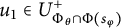 $u_1\in U_{\Phi _{\theta }\cap \Phi (s_{\varphi })}^+$
and
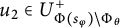 $u_2\in U_{\Phi (s_{\varphi })\backslash \Phi _{\theta }}^+$
, and so
 $ P_1s_{\varphi }^{-1}u^{-1}\theta us_{\varphi }P_1=P_1s_{\varphi }^{-1}u_2^{-1}\theta u_2s_{\varphi }P_1. $
Now,
 $\Phi (s_{\varphi })=\{\alpha \in \Phi ^+\mid \langle \alpha ,\omega _1\rangle \geq 1\}$
, and hence, by inspection of the root system, we have
 $ \Phi (s_{\varphi })\backslash \Phi _{\theta }=\{\alpha ,\beta ,\gamma ,\delta \}$
where
 $\alpha =(1111)$
,
 $\beta =(1121)$
,
 $\gamma =(1221)$
, and
 $\delta =(1231)$
. Writing
 $u_2=x_{\alpha }(a)x_{\beta }(b)x_{\gamma }(c)x_{\delta }(d)$
, a commutator relation calculation gives
 $$ \begin{align*} u_2^{-1}\theta u_2&=x_{\delta}(-d)x_{\gamma}(-c)x_{\beta}(-b)x_{\alpha}(-a)x_{\alpha}(-a)x_{\beta}(-b)x_{\gamma}(-c)x_{\delta}(-d)\theta\\ &=x_{\alpha}(-2a)x_{\beta}(-2b)x_{\gamma}(-2c)x_{\delta}(-2d)x_{\varphi}(-4ad+4bc)\theta. \end{align*} $$
Thus,
 $P_1s_{\varphi }^{-1}u^{-1}\theta us_{\varphi }P_1=P_1x_{-\delta }(-2a)x_{-\gamma }(2b)x_{-\beta }(-2c)x_{-\alpha }(2d)x_{-\varphi }(4ad-4bc)P_1$
. Easy calculations, using the folding relation and commutator relations, show that
 $x_{-\delta }(-2a)x_{-\gamma }(2b)x_{-\beta }(-2c)x_{-\alpha }(2d)x_{-\varphi }(4ad-4bc)$
is an element of
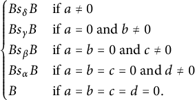 $$ \begin{align*} \begin{cases} Bs_{\delta}B&\text{if}\ a\neq 0\\ Bs_{\gamma}B&\text{if}\ a=0\ \text{and}\ b\neq 0\\ Bs_{\beta}B&\text{if}\ a=b=0\ \text{and}\ c\neq 0\\ Bs_{\alpha}B&\text{if}\ a=b=c=0\ \text{and}\ d\neq 0\\ B&\text{if}\ a=b=c=d=0. \end{cases} \end{align*} $$
Because
 $\beta =s_3\alpha $
,
 $\gamma =s_2s_3\alpha $
, and
 $\delta =s_3s_2s_3\alpha $
, we have
 $s_{\beta }=s_3s_{\alpha }s_3$
,
 $s_{\gamma }=s_2s_3s_{\alpha }s_3s_2$
and
 $s_{\delta }=s_3s_2s_3s_{\alpha }s_3s_2s_3$
, and hence
 $P_1s_{\alpha }P_1=P_1s_{\beta }P_1=P_1s_{\gamma }P_1=P_1s_{\delta }P_1$
. Thus,
 $$ \begin{align*}P_1s_{\varphi}^{-1}u^{-1}\theta us_{\varphi}P_1=\begin{cases} P_1s_{\alpha}P_1&\text{if}\ (a,b,d,c)\neq (0,0,0,0)\\ P_1&\text{if}\ (a,b,c,d)=(0,0,0,0). \end{cases} \end{align*} $$
We have
 $P_1s_{\alpha }P_1\neq P_1s_{\varphi }P_1$
. To see this, note that
 $s_{\alpha }=s_1s_2s_3s_4s_3s_2s_1$
(as
 $\alpha =s_1s_2s_3\alpha _4$
), and so both
 $s_{\alpha }$
and
 $s_{\varphi }$
are minimal length in their respective
 $W_1$
-double cosets (we noted above that
 $s_{\varphi }=w_0w_{\mathsf {C}_3}$
). But of course
 $s_{\alpha }\neq s_{\varphi }$
. Hence,
 $\theta $
is
 $\{1\}$
-domestic.▪
Theorem 5.9 Let
 $\theta $
be a nontrivial homology of
 $\mathsf {F}_4(\mathbb {F})$
. If
 $\mathrm {char}(\mathbb {F})=2$
, then
 $\theta $
is not domestic. If
 $\mathrm {char}(\mathbb {F})\neq 2$
, then
 $\theta $
is domestic if and only if
 $\Delta _{\theta }^{\prime }$
has type
 $\mathsf {B}_4$
. Moreover, all such homologies have opposition diagram
 $\mathsf {F}_{4;1}^4$
and are conjugate to
 $h_{\omega _4}(-1)$
.
Proof Let
 $\theta \in H$
, and suppose that
 $\Delta _{\theta }^{\prime }$
has type
 $\mathsf {B}_4$
. The simple roots of
 $\Phi _{\theta }$
are
 $ (\beta ,\alpha _1,\alpha _2,\alpha _3)$
, where
 $\beta =\alpha _2+2\alpha _3+2\alpha _4$
. Thus,
 $\theta =h_{\omega _4}(-1)$
(in particular,
 $\mathrm {char}(\mathbb {F})\neq 2$
). By Lemma 5.8,
 $\theta $
is domestic with diagram
 $\mathsf {F}_{4;1}^4$
.
We now use Lemma 5.3 to show that if
 $\theta \in H$
is a nontrivial homology with
 $\Delta _{\theta }^{\prime }$
not of type
 $\mathsf {B}_4$
, then
 $\theta $
is not domestic. It is sufficient to consider the cases:
-
(1)
$\Phi _{\theta }=\mathsf {C}_3\times \mathsf {A}_1$
, with simple roots
$(\alpha _4,\alpha _3,\alpha _2)\times (\varphi )$
, and
$\Phi _{\theta }^+=\{\alpha \in \Phi ^+\mid \langle \alpha ,\omega _1\rangle \in 2\mathbb {Z}\}$
. -
(2)
$\Phi _{\theta }=\mathsf {A}_2\times \mathsf {A}_2$
, with simple roots
$(\alpha _3,\alpha _4)\times (\alpha _1,\varphi -\alpha _1)$
, and
$\Phi _{\theta }^+=\{\alpha \in \Phi ^+\mid \langle \alpha ,\omega _2\rangle \in 3\mathbb {Z}\}$
. -
(3)
$\Phi _{\theta }=\mathsf {B}_3\times \mathsf {A}_1$
, with simple roots
$(\alpha _1,\alpha _2,\alpha _3)\times (\varphi ^{\prime })$
, and
$\Phi _{\theta }^+=\{\alpha \in \Phi ^+\mid \langle \alpha ,\omega _4\rangle =0\}\cup \{\varphi ^{\prime }\}$
. -
(4)
$\Phi _{\theta }=\mathsf {B}_2\times \mathsf {B}_2$
, with simple roots
$(\alpha _2,\alpha _3)\times (\beta ,\gamma )$
, where
$\beta =\alpha _2+2\alpha _3+2\alpha _4$
and
$\gamma =\alpha _1+\alpha _2+\alpha _3$
, and
$\Phi _{\theta }^+=\{\alpha _2,\alpha _3,\alpha _2+\alpha _3,\alpha _2+2\alpha _3,\beta ,\gamma ,\varphi ^{\prime },\varphi \}$
. -
(5)
$\Phi _{\theta }=\mathsf {D}_4$
, with simple roots
$(\alpha _2+2\alpha _3+2\alpha _4,\alpha _1,\alpha _2,\alpha _2+2\alpha _3)$
, and
$\Phi _{\theta }^+=\{\alpha \in \Phi ^+\mid \langle \alpha ,\omega _4\rangle \in 2\mathbb {Z}\text { and }\langle \alpha ,\omega _3\rangle \in 2\mathbb {Z}\}$
.

















In cases (1) and (2), we have
 $\beta _1,\beta _2,\beta _3\notin \Phi _{\theta }$
, where
 $\beta _1=(1220)$
,
 $\beta _2=(1222)$
, and
 $\beta _3=(1242)$
. The roots
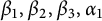 $\beta _1,\beta _2,\beta _3,\alpha _1$
are mutually perpendicular, and hence
 $s_{\beta _1}s_{\beta _2}s_{\beta _3}=w_0s_1$
by Lemma 2.2, and so by Lemma 5.3
 $\theta $
is not domestic.
In cases (3)–(5), we have
 $\gamma _1,\gamma _2,\gamma _3,\gamma _4\notin \Phi _{\theta }$
, where
 $\gamma _1=(0011)$
,
 $\gamma _2=(0111)$
,
 $\gamma _3=(1111)$
, and
 $\gamma _4=(1231)$
. Thus, again,
 $\theta $
is not domestic.▪
For the
 $\mathsf {G}_2$
results, see Theorem 7.10.
6 The polar–copolar type for
$\mathsf {E}_7$
,
$\mathsf {E}_8$
, and
$\mathsf {F}_4$


In this section, we prove Theorem 4, classifying the automorphisms with polar–copolar diagram in types
 $\mathsf {E}_7$
,
 $\mathsf {E}_8$
, and
 $\mathsf {F}_4$
. The arguments here are of a more geometric flavor, working in long root geometries and the metasymplectic space
 $\mathsf {F}_{4,4}(\mathbb {F})$
. See Section 2.5 for some relevant terminology, and see [Reference Shult21, Chapter 13] for further details.
Recall, from [Reference Parkinson and Van Maldeghem15], that if x is a simplex of a spherical building mapped onto an opposite simplex by an automorphism
 $\theta $
, then we write
 $\theta _{x}$
for the automorphism of the residue
 $\mathrm {Res}(x)$
given by
 $\theta _{x}=\mathrm {proj}_{x}\circ \theta $
, where
 $\mathrm {proj}_{x}$
is the projection from
 $\mathrm {Res}(x^{\theta })$
onto
 $\mathrm {Res}(x)$
. If
 $\xi $
is a simplex of
 $\mathrm {Res}(x)$
, then
 $\xi $
and
 $\xi ^{\theta }$
are opposite in
 $\Delta $
if and only if
 $\xi $
and
 $\xi ^{\theta _{x}}$
are opposite in the building
 $\mathrm {Res}(x)$
(see [Reference Tits28, Proposition 3.29]).
Note also that a long root elation fixes all points collinear and symplectic to a certain (unique) point c of the long root geometry, and c is called the center of the elation.
Our first task is to prove the following theorem (giving the “only if” direction of Theorem 4).
Theorem 6.1 A collineation belonging to a polar–copolar opposition diagram of a split exceptional building
 $\Delta $
not of type
 $\mathsf {E}_6$
if
 $\Delta $
is large, and not of type
 $\mathsf {E}_7$
or
 $\mathsf {E}_8$
if
 $\Delta $
is small, is the product of two orthogonal root elations. That is, the centers of the elations form a symplectic pair of points in the corresponding long root geometry.
Large buildings of type
 $\mathsf {E}_6$
are true exceptions to the theorem, for there exist homologies with the diagram
 ${^2}\mathsf {E}_{6;2}$
(see Theorem 5.4). For the small buildings of type
 $\mathsf {E}_i$
,
 $i=7,8$
, we believe that the theorem still holds; however, the geometric arguments break down.
The theorem follows from a series of lemmas. First, we need some properties of long root elations in the long root geometries
 $\mathsf {E}_{7,1}(\mathbb {F})$
,
 $\mathsf {D}_{6,2}(\mathbb {F})$
,
 $\mathsf {A}_{5,\{1,5\}}(\mathbb {F})$
, and
 $\mathsf {C}_{3,1}(\mathbb {F})$
. In these Lie incidence geometries, a vertex of the corresponding building of types
 $7$
,
 $6$
,
 $3$
, and
 $3$
, respectively, defines a (residual) sub-Lie incidence geometry, which we shall call a para, of types
 $\mathsf {E}_{6,1}(\mathbb {F})$
,
 $\mathsf {A}_{5,2}(\mathbb {F})$
,
 $\mathsf {A}_{2,1}\times \mathsf {A}_{2,1}(\mathbb {F})$
, and
 $\mathsf {A}_{2,1}(\mathbb {F})$
, respectively. The paras are also the points of the Lie incidence geometries
 $\mathsf {E}_{7,7}(\mathbb {F})$
,
 $\mathsf {D}_{6,6}(\mathbb {F})$
,
 $\mathsf {A}_{5,3}(\mathbb {F})$
, and
 $\mathsf {C}_{3,3}(\mathbb {F})$
, respectively. We call two paras adjacent if the corresponding points in the latter Lie incidence geometries are collinear. A pencil of paras corresponds to a line of that geometry.
Lemma 6.2 A long root elation
 $\theta $
of
 $\mathsf {E}_{7,1}(\mathbb {F})$
,
 $\mathsf {D}_{6,2}(\mathbb {F})$
,
 $\mathsf {A}_{5,\{1,5\}}(\mathbb {F})$
, and
 $\mathsf {C}_{3,1}(\mathbb {F})$
maps each nonfixed para P to an adjacent one, preserving the pencil defined by P and
 $P^\theta $
and fixing exactly one para of that pencil.
Proof A central elation in one of the Lie incidence geometries
 $\mathsf {E}_{7,7}(\mathbb {F})$
,
 $\mathsf {D}_{6,6}(\mathbb {F})$
,
 $\mathsf {A}_{5,3}(\mathbb {F})$
, and
 $\mathsf {C}_{3,3}(\mathbb {F})$
fixes all points of a “central” symp (which corresponds to the center of the elation), all points collinear to a maximal singular subspace of that symp, and all lines intersecting that symp in a point. Because every point that is not fixed is on exactly one such line, the lemma follows.▪
Let
 $\theta $
be a collineation with an exceptional polar–copolar opposition diagram of a large building. Let
 $\mathscr {G}$
be the corresponding long root geometry, and let
 $(p,\omega )$
be an incident point-symp pair which is mapped onto an opposite by
 $\theta $
.
Let
 $E(p,p^\theta )$
be the equator geometry of the pair
 $(p,p^\theta )$
, that is, the geometry induced by the points which are symplectic to both p and
 $p^\theta $
. For
 $\mathscr {G}$
of types
 $\mathsf {E}_{8,8}$
,
 $\mathsf {E}_{7,1}$
,
 $\mathsf {E}_{6,2}$
, and
 $\mathsf {F}_{4,1}$
, note that
 $E(p,p^\theta )$
is isomorphic to the long root geometry
 $\mathscr {G}^{\prime }$
of types
 $\mathsf {E}_{7,1}$
,
 $\mathsf {D}_{6,2}$
,
 $\mathsf {A}_{5,\{1,5\}}$
, and
 $\mathsf {C}_{3,1}$
, respectively. Moreover, symps, planes, and lines of
 $\mathscr {G}$
through p correspond to points, symps, and paras, respectively, of
 $\mathscr {G}^{\prime }$
. The case
 $(\mathsf {F}_{4,1},\mathsf {C}_{3,1})$
is special in that the lines of
 $\mathsf {C}_{3,1}(\mathbb {F})$
correspond to points of a symp in
 $E(p,p^\theta )$
(in this case,
 $E(p,p^\theta )$
does not contain lines; only symplectic and opposite pairs of points).
Lemma 6.3 Let
 $\theta $
and p be as above. Then,
 $\theta $
preserves
 $E(p,p^\theta )$
and induces a long root elation in it, say with center the point c.
Proof Recall that the symbol
 $\perp \!\!\!\perp $
means “symplectic to,” and
 $\Join $
“special to.”
Let
 $\pi $
be a plane through p fixed by
 $\theta _p$
. We claim that the line
 $\pi \cap (p^\theta )^{\Join }$
is mapped onto the line
 $\pi ^\theta \cap p^{\Join }$
. Indeed, first, assume that every line L through p in
 $\pi $
is fixed under
 $\theta _p$
, the alternative being that exactly one such line is fixed (by Lemma 6.2). Let M be the line in
 $\pi $
such that
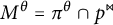 $M^\theta =\pi ^\theta \cap p^{\Join }$
. If
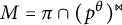 $M=\pi \cap (p^\theta )^{\Join }$
, then there is nothing to prove, so suppose M and
 $\pi \cap (p^\theta )^{\Join }$
intersect in a unique point z. Then, because
 $(pz)^{\theta _p}=pz$
, we see that
 $z^\theta \perp z$
. Now, let L be a line in
 $\pi $
through p, but not through z. Because
 $|\mathbb {F}|>2$
, we can select a point
 $q\in L\setminus (\{p\}\cup M\cup {p^\theta }^{\Join })$
. Let K be a line in
 $\pi $
through q, and set
 $K\cap M=\{u\}$
,
 $pu\cap (p^\theta )^{\Join }=\{v\}$
and
 $K\cap (p^\theta )^{\Join }=\{w\}$
. Because
 $(pv)^{\theta _p}=pv$
, we have
 $v\perp u^\theta $
. Hence,
 $(qu)^{\theta _q}=(qw)^{\theta _q}=qv$
. This now yields the equivalence
 $$ \begin{align*}(qw)^{\theta_q}=qw \Leftrightarrow v=w \Leftrightarrow u=z\mbox{ or } u\in pq.\end{align*} $$
Consequently, the central elation
 $\theta _q$
fixes
 $\pi $
and exactly two lines through q in
 $\pi $
, which contradicts Lemma 6.2, recalling that the lines through q correspond to the paras in that lemma.
Next, assume that exactly one line L through p in
 $\pi $
is fixed under
 $\theta _p$
. Because every such fixed line is contained in a fixed plane all of whose lines through p are fixed, we know by the previous paragraph that
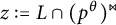 $z:=L\cap (p^\theta )^{\Join }$
is mapped onto
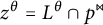 $z^\theta =L^\theta \cap p^{\Join }$
, and these two points are collinear. Let M again be the line of
 $\pi $
defined by
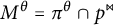 $M^\theta =\pi ^\theta \cap p^{\Join }$
. Let, for each
 $x\in M$
,
 $x^{\prime }$
be the unique point of
 $\pi $
collinear to
 $x^\theta $
, then, as a product of a linear collineation and a projection, the correspondence
 $x\mapsto x^{\prime }$
is a projectivity from M to
 $M^{\prime }:=\pi \cap (p^\theta )^{\Join }$
. Because
 $z=M\cap M^{\prime }$
is fixed under this correspondence, it is a perspectivity. Let c be the center of this perspectivity, then
 $c\notin M\cup M^{\prime }$
is opposite
 $c^\theta $
, and clearly,
 $\theta _c$
is the identity restricted to
 $\pi $
. By the first case, this implies that
 $M^{\prime }=M$
.
Now, let
 $\xi $
be an arbitrary symp through p. Every point of
 $\xi $
at distance
 $2$
from
 $p^\theta $
is collinear to the unique point
 $e_\xi $
of
 $\xi $
symplectic to
 $p^\theta $
, which is also the unique point of
 $\xi $
belonging to
 $E(p,p^\theta )$
. Hence, the previous claim can be formulated as:
 $\theta $
maps
 $p^\perp \cap e_\xi ^\perp $
to
 $(p^\theta )^\perp \cap e_{\xi ^\theta }^\perp $
. If
 $\xi $
is hyperbolic, or parabolic in uneven characteristic, then
 $p^\theta $
and
 $e_{\xi ^\theta }$
are the only two points of
 $\xi ^\theta $
collinear to all points of
 $(p^\theta )^\perp \cap e_{\xi ^\theta }^\perp $
; it follows that
 $e_\xi ^\theta =e_{\xi ^\theta }$
.
Now, suppose that
 $\xi $
is parabolic in characteristic 2. The foregoing implies that
 $\theta $
stabilizes the extended equator geometry
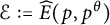 $\mathcal {E}:=\widehat {E}(p,p^\theta )$
(by definition, this is the union of all equator geometries
 $E(x,y)$
for
 $x,y$
opposite points in
 $E(p,p^{\theta })$
). Our assumption on p readily implies that
 $\theta $
acts plane-domestically but not line-domestically on
 $\mathcal {E}$
. Because
 $\mathcal {E}$
is a symplectic polar space of rank 4, the fixed point set of
 $\theta $
in
 $\mathcal {E}$
is of the form
 $u^{\perp \!\!\!\perp }\cap v^{\perp \!\!\!\perp }$
for two points
 $u,v$
of
 $\mathcal {E}$
. If
 $u\perp \!\!\!\perp v$
(in
 $\Delta $
), then
 $\theta $
is involutive on
 $\mathcal {E}$
and so preserves
 $E(p,p^\theta )$
. Otherwise,
 $\theta $
pointwise fixes
 $E(u,v)\subseteq \widehat {E}(p,p^\theta )$
. It follows that the fixed point set of the symp
 $\zeta $
determined by two symplectic points
 $x,y$
of
 $E(u,v)$
is exactly the imaginary line
 $E(u,v)\cap \zeta $
. This yields a plane
 $\pi $
of
 $\zeta $
disjoint from
 $\pi ^\theta $
. But then, every plane disjoint from
 $\pi $
and contained in a common symp with
 $\pi $
is mapped onto an opposite plane, a contradiction.
Hence, we have shown that
 $E(p,p^\theta )$
is preserved under the action of
 $\theta $
, and the lemma now follows from Theorem 1 for
 $\mathsf {E}_7(\mathbb {K})$
,
 $\mathsf {D}_{6}(\mathbb {K})$
, and
 $\mathsf {C}_{3}(\mathbb {K})$
.▪
Let
 $\theta $
, p, and
 $\omega $
be as above, and let
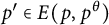 $p^{\prime }\in E(p,p^\theta )$
correspond to
 $\omega $
. Then,
 $p^{\prime }$
is opposite
 ${p^{\prime }}^\theta $
, and hence
 $E(p^{\prime },{p^{\prime }}^\theta )$
is preserved by
 $\theta $
. Because
 $p^{\prime }\in \omega $
, we can apply Lemma 6.3 and obtain that
 $\theta $
induces a long root elation in
 $E(p^{\prime },{p^{\prime }}^\theta )$
, say with center
 $c^{\prime }$
. Now, set
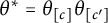 $\theta ^*=\theta _{[c]}\theta _{[c^{\prime }]}$
, with
 $\theta _{[c]}$
the central elation with center c (and similar for
 $\theta _{[c^{\prime }]}$
). Then,
 $\theta ^*\theta ^{-1}$
fixes every point of
 $E(p,p^\theta )\cup E(p^{\prime },{p^{\prime }}^\theta )$
(use the fact that, in
 $E(p,p^\theta )$
,
 $(\theta _{[c]})_{p^{\prime }}$
fixes
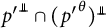 ${p^{\prime }}^{\perp \!\!\!\perp }\cap ({p^{\prime }}^\theta )^{\perp \!\!\!\perp }$
, which precisely coincides with
 $E(p,p^\theta )\cap E(p^{\prime },{p^{\prime }}^\theta )$
).
Now, Theorem 6.1 follows from the following general proposition.
Proposition 6.4 No nontrivial collineation of the long root geometry of (split) type
 $\mathsf {B}_n$
(
 $n\geq 4$
),
 $\mathsf {C}_n$
(
 $n\geq 3$
),
 $\mathsf {D}_n (n\geq 5$
),
 $\mathsf {E}_n$
(
 $8\geq n\geq 6$
), or
 $\mathsf {F}_4$
fixes two perpendicular equator geometries pointwise.
Proof For the classical types
 $\mathsf {B}/\mathsf {C}/\mathsf {D}$
, this follows from the easy fact that an equator geometry spans a subspace of dimension
 $n-4/n-2/n-4$
of the ambient projective space
 $\mathsf {PG}(n,\mathbb {F})$
,
 $n\geq 8/5/9$
, respectively; hence, if a collineation
 $\theta $
pointwise fixes two perpendicular equator geometries, then it fixes all points of two subspaces of dimension
 $n-4/n-2/n-4$
of
 $\mathsf {PG}(n,\mathbb {F})$
, spanning
 $\mathsf {PG}(n,\mathbb {F})$
,
 $n\geq 8/5/9$
, and hence intersecting in at least one point, and so forcing
 $\theta $
to be the identity.
Now, consider the long root geometries of type
 $\mathsf {E}$
. Let
 $E_1,E_2$
be two perpendicular equator geometries, that is,
 $E_1$
is the equator geometry
 $E(p_2,q_2)$
for
 $p_2,q_2\in E_2$
and
 $E_2=E(p_1,q_1)$
with
 $p_1,q_1\in E_1$
. Because
 $E_2$
is fixed pointwise,
 $\operatorname {{\mathrm {Res}}}(p_1)$
is fixed pointwise. Hence, every symp
 $\xi $
through
 $p_1$
is fixed, and every line in
 $\xi $
through
 $p_1$
is fixed. Moreover, the point
 $\xi \cap E_2$
, which is opposite
 $p_2$
in
 $\xi $
, is fixed. Because
 $\xi $
is hyperbolic,
 $\xi $
is fixed pointwise as soon as some line in
 $\xi $
through
 $p_1$
is fixed pointwise. By connectivity and the arbitrariness of
 $\xi $
, it suffices that some line through
 $p_1$
is fixed pointwise, which is the case as
 $E_1$
contains a line through
 $p_1$
and is fixed pointwise. Hence, all points collinear or symplectic to
 $p_1$
are fixed, and so we have a central elation with center
 $p_1$
. But the same thing holds for
 $q_1$
, and hence we have the identity.
At last, assume we have the long root geometry of type
 $\mathsf {F}_4$
. The same argument as in the previous paragraph shows that it suffices to find one line through
 $p_1$
that is pointwise fixed. To that aim, let
 $p_1^{\prime }\in E_1$
be such that
 $p_1\perp \!\!\!\perp p_1^{\prime }$
. Then, the symp
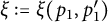 $\xi :=\xi (p_1,p_1^{\prime })$
corresponds to planes
 $\pi _p$
and
 $\pi _q$
through the points
 $p_2$
and
 $q_2$
, respectively. Then, the lines
 $L:=\pi _p\cap q_2^{\Join }$
and
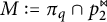 $M:=\pi _q\cap p_2^{\Join }$
are fixed and the points of
 $L^\perp \cap M^\perp $
belong to
 $E_1$
. Hence,
 $(p_1^\perp \cap {p_1^{\prime }}^\perp )\cup (L^\perp \cap M^\perp )$
is fixed pointwise, which implies that
 $\xi $
is fixed pointwise (note that
 $p_1,p_1^{\prime }\in L^\perp \cap M^\perp $
).
The proposition is proved.▪
The proof of Theorem 6.1 is complete, and the following theorem proves the “if” direction of Theorem 4.
Theorem 6.5 Every product of two perpendicular long root elations in
 $\mathsf {F}_4(\mathbb {F})$
(respectively
 $\mathsf {E}_{7}(\mathbb {F})$
,
 $\mathsf {E}_8(\mathbb {F})$
) is domestic with opposition diagram
 $\mathsf {F}_{4;2}$
(respectively
 $\mathsf {E}_{7;2}$
,
 $\mathsf {E}_{8;2}$
).
Proof Consider the
 $\mathsf {F}_4$
case. We claim that all pairs
 $(\alpha ,\beta )$
of perpendicular long roots are conjugate under W. Because W is transitive on long roots, it suffices to show that the stabilizer
 $W_{\varphi }$
of
 $\varphi $
in W is transitive on the set of long roots perpendicular to
 $\varphi $
. These roots are precisely the long roots of the
 $\mathsf {C}_3$
subsystem, and because
 $W_{\varphi }=\langle s_2,s_3,s_4\rangle =W_{\mathsf {C}_3}$
, the result follows. Hence, we may assume that
 $\theta =x_{\varphi }(a)x_{\varphi _{\mathsf {C}_3}}(b)$
, and then the result follows from Theorem 4.1. The arguments for
 $\mathsf {E}_7$
and
 $\mathsf {E}_8$
are similar.▪
7 Domestic automorphisms in split types
$\mathsf {E}_6$
,
$\mathsf {F}_4$
, and
$\mathsf {G}_2$


In this section, we give the complete classification of domestic automorphisms of split buildings of types
 $\mathsf {E}_6$
,
 $\mathsf {F}_4$
, and
 $\mathsf {G}_2$
.
7.1 Classification of domestic automorphisms of split
$\mathsf {F}_4$

In this section, we classify domestic automorphisms of split
 $\mathsf {F}_4$
buildings. By [Reference Parkinson and Van Maldeghem15, Lemma 4.1], no duality of a thick
 $\mathsf {F}_4$
building is domestic, and so we may restrict to collineations. The complete list of domestic collineations of the small building
 $\mathsf {F}_4(\mathbb {F}_2)$
is given in [Reference Parkinson and Van Maldeghem16, Theorem 4.3], and so we may assume that
 $|\mathbb {F}|>2$
, and so all automorphisms are capped. Thus, the possible opposition diagrams of nontrivial domestic collineations are
 $\mathsf {F}_{4;1}^1$
,
 $\mathsf {F}_{4;1}^4$
, and
 $\mathsf {F}_{4;2}$
. The automorphisms with diagram
 $\mathsf {F}_{4;1}^1$
are the long root elations (see Theorem 1), and the collineations with diagram
 $\mathsf {F}_{4;2}$
are products of perpendicular root elations (see Theorem 4). Thus, our main task is to consider the diagram
 $\mathsf {F}_{4;1}^4$
.
We will prove the following theorem.
Theorem 7.1 Let
 $\theta $
be an automorphism of
 $\Delta _{\mathsf {F}_4}(\mathbb {F})$
with opposition diagram
 $\mathsf {F}_{4,1}^4$
. If
 $\mathrm {char}(\mathbb {F})=2$
, then
 $\theta $
is a short root elation, and if
 $\mathrm {char}(\mathbb {F})\neq 2$
, then
 $\theta $
is a homology.
Let
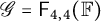 $\mathscr {G}=\mathsf {F}_{4,4}(\mathbb {F})$
be the short root geometry of the building
 $\Delta $
of
 $\mathsf {F}_4(\mathbb {F})$
. Then,
 $\mathscr {G}$
is a metasymplectic space with symps isomorphic to a symplectic polar space of rank 3 (see [Reference Shult21, Chapter 18] for details). If
 $\theta $
is a domestic collineation with opposition diagram
 $\mathsf {F}_{4;1}^4$
, then the only objects mapped to opposite objects are points.
Recall from [Reference De Schepper, Sastry and Van Maldeghem7, Section 5.2] that two opposite points
 $p,q$
in
 $\mathscr {G}$
define a geometry
 $\widehat {E}(p,q)$
of type
 $\mathsf {B}_4$
as follows: Let
 $E(p,q)$
denote the equator geometry of
 $p,q$
(as in Section 6), and take
 $\widehat {E}(p,q)$
to be the union of all equator geometries
 $E(x,y)$
for
 $x,y$
opposite points in
 $E(p,q)$
. The lines of
 $\widehat {E}(p,q)$
are the intersections of
 $\widehat {E}(p,q)$
with the symps
 $\xi (u,v)$
, with
 $\{u,v\}$
symplectic pairs in
 $\widehat {E}(p,q)$
. These intersections are imaginary lines of symplectic polar spaces. Note that two lines of
 $\widehat {E}(p,q)$
are opposite (as polar space lines) if and only if the corresponding symps are opposite in
 $\mathscr {G}$
.
Lemma 7.2 Let p be a point of
 $\mathscr {G}$
mapped onto an opposite point. Then,
 $\theta $
pointwise fixes a geometric hyperplane of
 $\widehat {E}(p,p^\theta )$
.
Proof Let p be a point of
 $\mathscr {G}$
mapped onto an opposite. Then,
 $\theta _p$
is the identity. Because the identity automatically and trivially satisfies the properties of central elations mentioned in Lemma 6.2, it follows from the proof of Lemma 6.3 that
 $\theta $
pointwise fixes
 $E(p,p^\theta )$
. Hence,
 $\theta $
stabilizes
 $\widehat {E}(p,p^\theta )$
. Because (opposite) lines of
 $\widehat {E}(p,p^\theta )$
correspond to (opposite) symps in
 $\mathscr {G}$
,
 $\theta $
induces a line-domestic collineation in
 $\widehat {E}(p,p^\theta )$
. The assertion now follows from [Reference Temmermans, Thas and Van Maldeghem25, Theorem 5.1].▪
In the case that
 $\mathrm {char}(\mathbb {F})=2$
, we need a more precise version of the above lemma.
Lemma 7.3 Let p be a point mapped onto an opposite. If
 $\mathrm {char}(\mathbb {F})=2$
, then
 $\theta $
pointwise fixes either the perp of a point in
 $\widehat {E}(p,p^\theta )$
, or a subspace of
 $\widehat {E}(p,p^\theta )$
inducing a nondegenerate polar space of Witt index
 $3$
in
 $\widehat {E}(p,p^\theta )$
. In both cases,
 $p^{\theta ^2}=p$
.
Proof In this case,
 $\widehat {E}(p,p^\theta )$
may be identified with the polar space (of type
 $\mathsf {B_4}$
) obtained from the standard symplectic polar space in
 $\mathsf {PG}(7,\mathbb {F})$
with alternating form
 $x_0y_1+x_1y_0+\cdots +x_6y_7+x_7y_6$
by only considering the points whose coordinates
 $(x_0,\ldots ,x_7)$
satisfy
 $x_0x_1+x_2x_3+x_4x_5+x_6x_7\in \mathbb {F}^2$
, where the latter is the subfield of squares of
 $\mathbb {F}$
. Without loss, we may assume that
 $p=(0,0,\ldots ,1,0)$
is mapped onto
 $(0,\ldots ,0,1)$
. By Lemma 7.2 and its proof,
 $\theta $
fixes pointwise a hyperplane of
 $\mathsf {PG}(7,\mathbb {F})$
containing the subspace with equations
 $X_6=X_7=0$
. Hence, some point
 $t=(0,\ldots ,0,k,1)$
is fixed, with
 $k\in \mathbb {F}$
, along with all points having coordinates
 $(x_0,x_1,\ldots ,x_5,k,1)$
. If
 $k\in \mathbb {F}^2$
, then
 $t\in \widehat {E}(p,p^\theta )$
and
 $\theta $
fixes the perp of t. Then,
 $\theta $
is an elation in
 $\mathsf {PG}(7,\mathbb {F})$
and hence an involution on
 $\widehat {E}(p,p^\theta )$
.
Now, assume
 $k\notin \mathbb {F}^2$
. Let
 $a,b,c\in \mathbb {F}$
be defined by
 $$ \begin{align*}\theta:(x_0,\ldots,x_5,x_6,x_7)\mapsto (x_0,\ldots,x_5,ax_7,bx_6+cx_7).\end{align*} $$
Expressing that
 $(0,\ldots ,0,1,k,k,1)$
is fixed, we obtain
 $a=k$
and
 $c=kb+1$
. Expressing that the image of an arbitrary point of
 $\widehat {E}(p,p^\theta )$
stays inside of
 $\widehat {E}(p,p^\theta )$
, we get
 $bk=1$
, and so
 $\theta $
is involutive on
 $\widehat {E}(p,p^\theta )$
. Moreover, we can now project the fixed point set from
 $(0,\ldots ,0,k,1)$
onto the subspace
 $X_6=X_7=0$
and obtain the polar space whose points have coordinates
 $(x_0,x_1,\ldots ,x_5)$
with
 $x_0x_1+x_2x_3+x_4x_5\in \mathbb {F}^2+k\mathbb {F}^2$
. That is, a polar space of Witt index
 $3$
.▪
Lemma 7.4 Assume that
 $\mathrm {char}(\mathbb {F})=2$
, and suppose that whenever a point p is mapped onto an opposite point,
 $\theta $
pointwise fixes the perp of a point in
 $\widehat {E}(p,p^\theta )$
. Then,
 $\theta $
is a central elation.
Proof Let p be a point mapped onto an opposite, and suppose
 $\theta $
fixes all points of
 $\widehat {E}(p,p^\theta )$
symplectic to
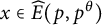 $x\in \widehat {E}(p,p^\theta )$
. Arguments similar to the ones in the proof of Proposition 6.4 show that all vertices of
 $\Delta $
incident with x are fixed by
 $\theta $
. Let y be opposite x in
 $\widehat {E}(p,p^\theta )$
. Then,
 $E(x,y)$
is fixed pointwise. Let
 $y^{\prime }\perp y$
be also opposite x. Then, we have a unique path
 $y,yy^{\prime },b,ab,a,ax,x$
of consecutively incident points and lines connecting y with x using the line
 $yy^{\prime }$
. Because
 $x,y,y^\theta $
are on the same imaginary line, and because
 $ax$
is fixed, we see that
 $(ab)^\theta =ab$
(this also follows from the fact that the line
 $ab$
defines a unique plane of
 ${E}(p,p^\theta )$
,which is fixed; see [Reference De Schepper, Sastry and Van Maldeghem7, Proposition 5.3.9]). Hence, the unique point
 $x^{\prime }$
on
 $ax$
and on the imaginary line determined by
 $y^{\prime }$
and
 ${y^{\prime }}^\theta $
is fixed. If
 $x\neq x^{\prime }$
, then, because
 $\theta $
acts linearly (as it pointwise fixes
 $E(p,p^\theta )$
), it fixes all points of
 $ax$
, and the arguments in the proof of Lemma 6.4 then imply that all points collinear to x are fixed. Otherwise,
 $x=x^{\prime }$
, and
 $E(x,y^{\prime })$
is fixed pointwise, again implying that at least one line through x is fixed pointwise, and hence, as before, all of them are. In addition, as before in the proof of Lemma 6.4, it follows now that all points collinear or symplectic to x are fixed, and so
 $\theta $
is a central elation with center x.▪
Lemma 7.5 If a point p is mapped onto a collinear point
 $p^\theta \neq p$
, then the line
 $pp^\theta $
is fixed under
 $\theta $
.
Proof In
 $\operatorname {{\mathrm {Res}}}_\Delta (p^\theta )$
, we find a line L opposite both
 $pp^\theta $
and
 $(pp^\theta )^\theta $
. Then, any point x on
 $L^{\theta ^{-1}}$
distinct from p is mapped onto an opposite. Then,
 $E(x,x^\theta )$
is fixed pointwise. If
 $\mathrm {char}(\mathbb {F})\neq 2$
, the points x and
 $x^\theta $
are the only points of
 $\widehat {E}(x,x^\theta )$
symplectic to all points of
 $E(x,x^\theta )$
. It follows that
 $(x^\theta )^\theta =x$
. If
 $\mathrm {char}(\mathbb {F})=2$
, the latter follows directly from Lemma 7.3. In addition, each line through x is mapped onto its projection on
 $x^\theta $
, so
 $xp$
is mapped onto
 $x^\theta p^\theta $
and vice versa, and so
 $(p^\theta )^\theta =p$
and the line
 $pp^\theta $
is fixed.▪
Lemma 7.6 Suppose
 $\mathrm {char}(\mathbb {F})\neq 2$
, or that
 $\mathrm {char}(\mathbb {F})=2$
and that for at least one point x mapped onto an opposite, the fixed point structure induced by
 $\theta $
in
 $\widehat {E}(x,x^\theta )$
is a nondegenerate polar space. Then, necessarily,
 $\mathrm {char}(\mathbb {F})\neq 2$
, and there exists an apartment
 $\Sigma $
of
 $\Delta $
fixed pointwise by
 $\theta $
. In addition,
 $\theta $
fixes some panel pointwise and hence is a homology.
Proof Let
 $p,q$
be two fixed (by
 $\theta $
) opposite points such that
 $\theta $
fixes pointwise a geometric hyperplane H of
 $\widehat {E}(p,q)$
(see Lemma 7.2). If
 $\mathrm {char}(\mathbb {F})=2$
, we may assume that H is a nondegenerate polar space of Witt index 3. If
 $\mathrm {char}(\mathbb {F})\neq 2$
, the hyperplane is not singular (if a collineation fixes all points collinear to a given point of a parabolic polar space, then it is the identity). Hence, H is a subquadric either of Witt index 4 (of type
 $\mathsf {D}_4$
), or of Witt index 3. Now, assume for a contradiction that H has Witt index 3 (in either characteristic).
Let
 $\pi $
be a plane of
 $\widehat {E}(p,q)$
. Then, by [Reference De Schepper, Sastry and Van Maldeghem7, Corollary 5.3.7], there is a unique point
 $p_U$
collinear to each
 $3$
-space U of
 $\widehat {E}(p,q)$
containing
 $\pi $
. Moreover, Proposition 5.3.9 of [Reference De Schepper, Sastry and Van Maldeghem7] implies that the set of all such points
 $p_U$
, for U running through all
 $3$
-spaces of
 $\widehat {E}(p,q)$
containing
 $\pi $
, forms a line
 $L_\pi $
of
 $\Delta $
. Because
 $\pi $
is fixed, the line
 $L_\pi $
is also fixed by
 $\theta $
. Note that, because no
 $3$
-space of
 $\widehat {E}(p,q)$
is fixed, no point on
 $L_\pi $
is fixed. Select any point
 $x\in \pi $
. Then also the plane spanned by
 $L_\pi $
and x is fixed by
 $\theta $
. Hence an arbitrary point
 $z\in \pi \setminus (\{x\}\cup L_\pi )$
is either fixed or mapped to a collinear point. In the former case, the point
 $L_\pi \cap xz$
is fixed, and in the latter case, the point
 $L_\pi \cap zz^\theta $
is fixed (use Lemma 7.5), twice the same contradiction.
Hence, H has Witt index 4 (and
 $\mathrm {char}(\mathbb {F})\neq 2$
). Select two opposite points
 $x_0,x_1$
in
 $\widehat {E}(p,q)$
, fixed by
 $\theta $
. Select two opposite points
 $y_0,y_1\in \{x_0,x_1\}^{\perp \!\!\!\perp }$
, again fixed by
 $\theta $
. Set
 $\xi _i:=\xi (x_i,y_i)$
,
 $i=1,2$
. Then,
 $\xi _0$
is opposite
 $x_1$
. Select lines
 $L_0,L_1$
and planes
 $\pi _0,\pi _1$
in
 ${E}(x_0,x_1)$
such that
 $y_i\in L_i\subseteq \pi _i$
,
 $i=0,1$
, and
 $L_0$
is opposite
 $L_1$
, whereas
 $\pi _0$
is opposite
 $\pi _1$
in the polar space
 $\widehat {E}(p,q)$
, and
 $L_0,L_1,\pi _0,\pi _1$
are fixed by
 $\theta $
. To the pair,
 $L_i$
 $\pi _i$
there corresponds a plane
 $\alpha _i$
and a line
 $K_i$
through
 $x_i$
, with
 $K_i\subseteq \alpha _i\subseteq \xi _i$
,
 $i=0,1$
, and
 $K_0$
is opposite
 $K_1$
, whereas
 $\alpha _0$
is opposite
 $\alpha _1$
. Hence, the chambers
 $\{x_0,K_0,\alpha _0,\xi _0\}$
and
 $\{x_1,K_1,\alpha _1,\xi _1\}$
are fixed and opposite, and so they uniquely determine a pointwise fixed apartment
 $\Sigma $
.
With the notation of the previous paragraph, it is clear that
 $\theta $
fixes all lines in
 $\pi _0$
through
 $y_0$
. Hence, the panel determined by
 $\{x_0,K_0,\xi _0\}$
is fixed pointwise by
 $\theta $
.▪
The proof of Theorem 7.1 is now complete. We note the following corollary (completing a postponed part of the proof of Theorem 3.10). Let
 $\varphi ^{\prime }$
be the highest short root of the
 $\mathsf {F}_4$
root system.
Corollary 7.7 In
 $\mathsf {F}_4(\mathbb {F})$
, the element
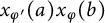 $x_{\varphi ^{\prime }}(a)x_{\varphi }(b)$
with
 $a,b\neq 0$
has opposition diagram
 $\mathsf {F}_{4;2}$
. If
 $\mathrm {char}(\mathbb {F})\neq 2$
, then
 $x_{\varphi ^{\prime }}(a)$
has this diagram too, and if
 $\mathrm {char}(\mathbb {F})=2$
, then it has diagram
 $\mathsf {F}_{4;1}^4$
.
Proof By the angle between root elations
 $x_{\alpha }(a)$
and
 $x_{\beta }(b)$
, we shall mean the angle between the roots
 $\alpha $
and
 $\beta $
. We claim that:
-
(1) Every product of a short root elation and a long root elation at angle
$\pi /4$
is conjugate to a product of two perpendicular long root elations. -
(2) If
$\mathrm {char}(\mathbb {F})\neq 2$
, then every short root elation is conjugate to a product of two perpendicular long root elations.


To begin with, note that the Weyl group is transitive on pairs
 $(\alpha ,\beta )$
with
 $\alpha $
short,
 $\beta $
long, and
 $\mathrm {angle}(\alpha ,\beta )=\pi /4$
. An example of such a pair is
 $(\varphi ^{\prime },\varphi )$
, and it is sufficient to show that the stabilizer
 $W_{\mathsf {C}_3}$
of
 $\varphi $
is transitive on the set of short roots with angle
 $\pi /4$
with
 $\varphi $
. These six roots are
 $(1110),(1111),(1121),(1221),(1231),(1232)$
, and an easy check shows that
 $W_{\mathsf {C}_3}$
is indeed transitive on these roots.
Thus, to prove (1), we may assume that
 $\theta =x_{\alpha }(a)x_{\beta }(b)$
with
 $\alpha =(1110)$
,
 $\beta =(1000)$
, and
 $a,b\neq 0$
. By commutator relations,
 $$ \begin{align*} x_{\alpha}(a)x_{\beta}(b)&=x_{\gamma}(ab^{-1})^{-1}x_{\delta}(a^2b^{-1})x_{\beta}(b)x_{\gamma}(ab^{-1}), \end{align*} $$
where
 $\gamma =(0110)$
and
 $\delta =(1220)$
. This proves (1), as
 $(\delta ,\beta )$
is a pair of perpendicular long roots.
Now, suppose that
 $\theta $
is a short root elation. After conjugating, we may assume that
 $\theta =x_{\varphi ^{\prime }}(a)$
for some
 $a\neq 0$
. Let
 $\epsilon =(1110)$
. By commutator relations, we have
 $$ \begin{align*}x_{\epsilon}(a^{-1}/2)\theta x_{\epsilon}(a^{-1}/2)^{-1}=x_{\varphi^{\prime}}(a)x_{\varphi}(1). \end{align*} $$
Note that
 $\varphi ^{\prime }$
is short,
 $\varphi $
is long, and
 $\mathrm {angle}(\varphi ^{\prime },\varphi )=\pi /4$
, and so applying the first statement completes the proof of the claims.
The statement of the corollary now follows from Theorem 4, and the fact that if
 $\mathsf {char}(\mathbb {F})=2$
, then the
 $\mathsf {F}_{4,4}(\mathbb {F})$
geometry isometrically embeds into the
 $\mathsf {F}_{4,1}(\mathbb {F})$
geometry, with short root elations becoming long root elations.▪
We now collect the results to prove Theorem 7.
Proof of Theorem 7. All that remains is to prove the statements concerning the number of conjugacy classes. If
 $\theta $
has diagram
 $\mathsf {F}_{4;1}^1$
, then
 $\theta $
is conjugate to
 $x_{\varphi }(a)$
for some
 $a\in \mathbb {F}$
(by Theorem 1). Then,
 $ h_{\omega _1-\omega _2}(a)x_{\varphi }(a)h_{\omega _1-\omega _2}(a)^{-1}=x_{\varphi }(1), $
and so all long root elations are conjugate.
If
 $\theta $
has diagram
 $\mathsf {F}_{4;1}^4$
, and
 $\mathrm {char}(\mathbb {F})\neq 2$
, then
 $\theta $
is conjugate to
 $h_{\omega _4}(-1)$
(by Theorems 5.9 and 7.1). If
 $\mathrm {char}(\mathbb {F})=2$
, then
 $\theta $
is conjugate to
 $x_{\varphi ^{\prime }}(1)$
(by Lemmas 7.4 and 7.6).
Thus, suppose that
 $\theta $
has diagram
 $\mathsf {F}_{4;2}$
. By the proof of Corollary 7.7, we may assume that
 $\theta =x_{\varphi }(a)x_{\varphi _{\mathsf {C}_3}}(b)$
, and conjugating by a diagonal element, we may take
 $a=1$
. If
 $b=c^2$
is a square, then
 $$ \begin{align*}h_{3\omega_1-2\omega_2}(c)x_{\varphi}(1)x_{\varphi_{\mathsf{C}_3}}(c^2)h_{3\omega_1-2\omega_2}(c)^{-1}=x_{\varphi}(1)x_{\varphi_{\mathsf{C}_3}}(1). \end{align*} $$
This shows that there is at most one conjugacy class for each element of the quotient
 $\mathbb {F}^{\times }/(\mathbb {F}^{\times })^2$
(where
 $(\mathbb {F}^{\times })^2=\{x^2\mid x\in \mathbb {F}^{\times }\}$
). Thus, if
 $\mathbb {F}$
is quadratically closed, then we conclude that there is a unique conjugacy class of automorphisms with diagram
 $\mathsf {F}_{4;2}$
. Similarly, if
 $\mathbb {F}$
is finite and
 $\mathrm {char}(\mathbb {F})=2$
, then there is a unique conjugacy class (as every element is a square). Finally, if
 $\mathbb {F}$
is finite with
 $\mathrm {char}(\mathbb {F})\neq 2$
, we conclude that there are at most two conjugacy classes, and by the tables in [Reference Liebeck and Seitz12], the elements
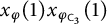 $x_{\varphi }(1)x_{\varphi _{\mathsf {C}_3}}(1)$
and
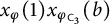 $x_{\varphi }(1)x_{\varphi _{\mathsf {C}_3}}(b)$
with
 $b\notin (\mathbb {F}^{\times })^2$
are not conjugate, and so there are precisely two classes.▪
7.2 Classification of domestic automorphisms of thick
$\mathsf {E}_6$
buildings

The classification of domestic automorphisms of the small
 $\mathsf {E}_6$
building (with
 $\mathbb {F}=\mathbb {F}_2$
) is given in [Reference Parkinson and Van Maldeghem16, Theorems 4.5 and 4.6], and the classification of domestic dualities of large
 $\mathsf {E}_6$
buildings is given in [Reference Van Maldeghem and Sastry32]. By Theorem 1, the collineations with diagram
 ${^2}\mathsf {E}_{6;1}$
are root elations, and so all that remains to complete the classification of domestic automorphisms of thick
 $\mathsf {E}_6$
buildings is to classify the collineations of large
 $\mathsf {E}_6$
buildings with diagram
 ${^2}\mathsf {E}_{6;2}$
.
We begin with some setup. Let
 $\varphi $
be the highest root of
 $\mathsf {E}_6$
, and let
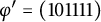 $\varphi ^{\prime }=(101111)$
be the highest root of the
 $\mathsf {A}_5$
subsystem. Let
 $\Phi _1$
be the
 $\mathsf {A}_3$
subsystem generated by the simple roots
 $\alpha _3,\alpha _4,\alpha _5$
, and let
 $\varphi ^{\prime \prime }=(001110)$
be the highest root of
 $\Phi _1$
.
Let
 $\beta _1=(100000)$
,
 $\beta _2=(010000)$
,
 $\beta _3=(000001)$
,
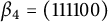 $\beta _4=(111100)$
,
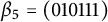 $\beta _5=(010111)$
, and
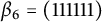 $\beta _6=(111111)$
, and for
 $1\leq i\leq 6$
, let
 $C_i=\{\alpha \in \Phi ^+\mid \alpha -\beta _i\in \mathbb {Z}_{\geq 0}\alpha _3+\mathbb {Z}_{\geq 0}\alpha _4+\mathbb {Z}_{\geq 0}\alpha _5\}$
. Explicitly, we have
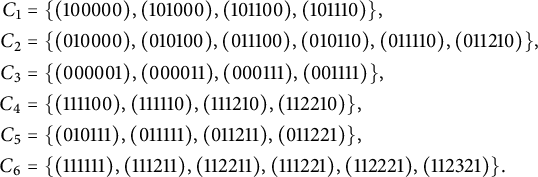 $$ \begin{align*} C_1&=\{(100000),(101000),(101100),(101110)\},\\ C_2&=\{(010000),(010100),(011100),(010110),(011110),(011210)\},\\ C_3&=\{(000001),(000011),(000111),(001111)\},\\ C_4&=\{(111100),(111110),(111210),(112210)\},\\ C_5&=\{(010111),(011111),(011211),(011221)\},\\ C_6&=\{(111111),(111211),(112211),(111221),(112221),(112321)\}. \end{align*} $$
Note that
 $\{C_i\mid 1\leq i\leq 6\}$
is a partition of
 $\Phi ^+\backslash (\Phi _1\cup \{\varphi ,\varphi ^{\prime }\})$
. For each
 $i=1,\ldots ,6$
, let
 $$ \begin{align*}C_i^{\prime}=(C_i \cup C_{i+1}\cup\cdots\cup C_6)\backslash\{\beta_i,\beta_i+\varphi''\}. \end{align*} $$
The following technical lemma is required.
Lemma 7.8 Let
 $1\leq i\leq 6$
, and suppose that
 $ u=u'x_{\beta _i+\varphi ''}(b)x_{\beta _i}(a) $
with
 $a\neq 0$
,
 $b\in \mathbb {F}$
, and
 $u^{\prime }$
a product of root elations with roots in
 $C_i^{\prime }$
. Let
 $z_1,z_2,c,d\in \mathbb {F}$
. If
 $z_2\neq 0$
and
 $bz_2\neq -1$
, then
 $$ \begin{align*}x_{-\beta_i-\varphi''}(z_1)x_{-\varphi}(1)x_{-\varphi'}(1)x_{\varphi}(c)x_{\varphi'}(d)ux_{-\beta_i-\varphi''}(z_2)\in Bw_0s_4B. \end{align*} $$
Proof We make the following two claims:
-
(1) If
$z_1,z_1^{\prime }\in \mathbb {F}$
, then
$Bx_{-\beta _i-\varphi ^{\prime \prime }}(z_1)x_{-\varphi }(1)x_{-\varphi ^{\prime }}(1)x_{\varphi }(c)x_{\varphi ^{\prime }}(d)x_{-\beta _i-\varphi ^{\prime \prime }}(z_1^{\prime })B= Bs_{\varphi }s_{\varphi ^{\prime }}B$
; -
(2) With
$z_3=(b+z_2^{-1})^{-1}$
, we have
$ux_{-\beta _i-\varphi ''}(z_2)B\in x_{-\beta _i-\varphi ''}(z_3)Bs_{\varphi ''}B$
.




The result follows from these claims, because writing
 $$ \begin{align*}g=x_{-\beta_i-\varphi''}(z_1)x_{-\varphi}(1)x_{-\varphi'}(1)x_{\varphi}(c)x_{\varphi'}(d)ux_{-\beta_i-\varphi''}(z_2),\end{align*} $$
and using (2) followed by (1) gives
 $$ \begin{align*} g&\in x_{-\beta_i-\varphi''}(z_1)x_{-\varphi}(1)x_{-\varphi'}(1)x_{\varphi}(c)x_{\varphi'}(d)x_{-\beta_i-\varphi''}(z_3)Bs_{\varphi''}B\\ &\subseteq Bs_{\varphi}s_{\varphi'}B\cdot Bs_{\varphi''}B\\ &=Bs_{\varphi}s_{\varphi'}s_{\varphi''}B=Bw_0s_4B, \end{align*} $$
where, for the final two equalities, we have used Lemma 4.5.
We prove (1). Let
 $X=Bx_{-\beta _i-\varphi ^{\prime \prime }}(z_1)x_{-\varphi }(1)x_{-\varphi ^{\prime }}(1)x_{\varphi }(c)x_{\varphi ^{\prime }}(d)x_{-\beta _i-\varphi ^{\prime \prime }}(z_1^{\prime })B$
. We will write
 $x_{\alpha }(\cdot )$
as shorthand for an element of
 $U_{\alpha }$
with the convention that
 $x_{\alpha }(\cdot )=1$
if
 $\alpha \notin \Phi $
. By commutator relations, and replacing
 $x_{-\varphi }(1)=x_{\varphi }(1)s_{\varphi }^{-1}x_{\varphi }(1)$
and similarly for
 $x_{-\varphi '}(1)$
, and noting that the roots
 $\varphi $
and
 $\varphi '$
are perpendicular, we compute
 $$ \begin{align*} X&=Bx_{-\varphi}(1)x_{-\varphi^{\prime}}(1)x_{-\varphi^{\prime}-\beta_i-\varphi^{\prime\prime}}(\cdot)x_{-\beta_i-\varphi^{\prime\prime}}(\cdot)x_{\varphi}(c)x_{\varphi^{\prime}}(d)x_{-\beta_i-\varphi^{\prime\prime}}(z_1^{\prime})B\\ &=Bs_{\varphi}s_{\varphi^{\prime}}x_{\varphi}(1)x_{\varphi^{\prime}}(1)x_{-\varphi^{\prime}-\beta_i-\varphi^{\prime\prime}}(\cdot)x_{-\beta_i-\varphi^{\prime\prime}}(\cdot)x_{\varphi^{\prime}-\beta_i-\varphi^{\prime\prime}}(\cdot)x_{\varphi-\beta_i-\varphi^{\prime\prime}}(\cdot)\\ &\quad\times x_{\varphi+\varphi^{\prime}-\beta_i-\varphi^{\prime\prime}}(\cdot)B. \end{align*} $$
Now, by inspection, both
 $\varphi -\beta _i-\varphi ''$
and
 $\varphi +\varphi '-\beta _i-\varphi ''$
are either not roots, or positive roots, and hence these terms can be absorbed into B. Thus,
 $$ \begin{align*} X&=Bs_{\varphi}s_{\varphi'}x_{\varphi}(1)x_{\varphi'}(1)x_{-\varphi'-\beta_i-\varphi''}(\cdot)x_{-\beta_i-\varphi''}(\cdot)x_{\varphi'-\beta_i-\varphi''}(\cdot)B. \end{align*} $$
Moreover, note that
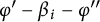 $\varphi '-\beta _i-\varphi ''$
is a negative root if and only if
 $i=6$
(in all other cases, it is either not a root, or a positive root, and hence can be absorbed into B). In addition, note that
 $-\varphi '-\beta _i-\varphi ''$
is only a root for
 $i=2$
.
We now push the
 $x_{\varphi }(1)x_{\varphi '}(1)$
term to the right, to be absorbed into the B. In the case
 $i\neq 2,6$
, this gives
 $X=Bs_{\varphi }s_{\varphi '}x_{-\beta _i-\varphi ''}(\cdot )B$
, and then because
 $\beta _i+\varphi ''\in \Phi (s_{\varphi }s_{\varphi '})=\Phi ^+\backslash \Phi _1$
, the term
 $x_{-\beta _i-\varphi ''}(\cdot )$
is absorbed into the B on the left-hand side after moving past
 $s_{\varphi }s_{\varphi '}$
. For
 $i=2$
, we compute
 $ X=Bs_{\varphi }s_{\varphi '}x_{-\varphi '-\beta _i-\varphi ''}(\cdot )x_{-\beta _i-\varphi ''}(\cdot )B$
, and because
 $\varphi '+\beta _i+\varphi ,''\beta _i+\varphi ''\in \Phi (s_{\varphi }s_{\varphi '})$
, the result again follows. Similarly, for
 $i=6$
, we compute
 $X=Bs_{\varphi }s_{\varphi '}x_{-\beta _i-\varphi ''}(\cdot )x_{\varphi '-\beta _i-\varphi ''}(\cdot )B$
. In this case,
 $\varphi '-\beta _i-\varphi ''=-(011110)$
, and so both roots
 $\beta _i+\varphi ''$
and
 $-\varphi '+\beta _i+\varphi ''$
are in
 $\Phi (s_{\varphi }s_{\varphi '})$
, and the result follows as before. Hence the claim.
We now prove (2). With
 $u'$
as in the statement of the theorem, we have
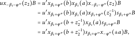 $$ \begin{align*} ux_{-\beta_i-\varphi''}(z_2)B&=u'x_{\beta_i+\varphi''}(b)x_{\beta_i}(a)x_{-\beta_i-\varphi''}(z_2)B\\ &=u'x_{\beta_i+\varphi''}(b)x_{\beta_i}(a)x_{\beta_i+\varphi''}(z_2^{-1})s_{\beta_i+\varphi''}B\\ &=u'x_{\beta_i+\varphi''}(b+z_2^{-1})x_{\beta_i}(a)s_{\beta_i+\varphi''}B\\ &=u'x_{\beta_i+\varphi''}(b+z_2^{-1})s_{\beta_i+\varphi''}x_{-\varphi''}(\pm a)B, \end{align*} $$
where we have used the facts that
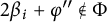 $2\beta _i+\varphi ''\notin \Phi $
and
 $s_{\beta _i+\varphi ''}(\beta _i)=-\varphi ''$
, for all
 $1\leq i\leq 6$
. Recalling that
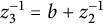 $z_3^{-1}=b+z_2^{-1}$
, using the folding relation, we have
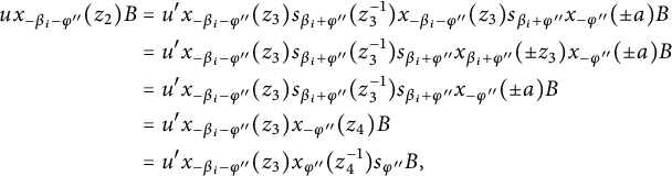 $$ \begin{align*} ux_{-\beta_i-\varphi''}(z_2)B&=u'x_{-\beta_i-\varphi''}(z_3)s_{\beta_i+\varphi''}(z_3^{-1})x_{-\beta_i-\varphi''}(z_3)s_{\beta_i+\varphi''}x_{-\varphi''}(\pm a)B\\ &=u'x_{-\beta_i-\varphi''}(z_3)s_{\beta_i+\varphi''}(z_3^{-1})s_{\beta_i+\varphi''}x_{\beta_i+\varphi''}(\pm z_3)x_{-\varphi''}(\pm a)B\\ &=u'x_{-\beta_i-\varphi''}(z_3)s_{\beta_i+\varphi''}(z_3^{-1})s_{\beta_i+\varphi''}x_{-\varphi''}(\pm a)B\\ &=u'x_{-\beta_i-\varphi''}(z_3)x_{-\varphi''}(z_4)B\\ &=u'x_{-\beta_i-\varphi''}(z_3)x_{\varphi''}(z_4^{-1})s_{\varphi''}B, \end{align*} $$
for some
 $z_4\neq 0$
.
By commutator relations, one may write
 $$ \begin{align*}u'x_{-\beta_i-\varphi''}(z_3)=x_{-\beta_i-\varphi''}(z_3)u'', \end{align*} $$
where
 $u^{\prime \prime }$
is a product of elements from root subgroups
 $U_{\gamma }$
with
 $\gamma \in Y_i$
, where
 $Y_i=\{\alpha ,\alpha -\beta _i-\varphi ^{\prime \prime }\mid \alpha \in C_i^{\prime }\}\cap \Phi $
. By inspection of the elements of
 $C_i^{\prime }$
, if
 $\gamma \in Y_i$
is a negative root, then necessarily
 $\gamma \in \Phi _1$
. Moreover, one sees that
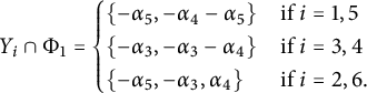 $$ \begin{align*} Y_i\cap \Phi_1= \begin{cases} \{-\alpha_5,-\alpha_4-\alpha_5\}&\text{if}\ i=1,5\\ \{-\alpha_3,-\alpha_3-\alpha_4\}&\text{if}\ i=3,4\\ \{-\alpha_5,-\alpha_3,\alpha_4\}&\text{if}\ i=2,6. \end{cases} \end{align*} $$
It follows that
 $u''$
can be written in the form
 $ u''=u'''y_i, $
where
 $u'''\in U^+$
and
 $y_i\in \prod _{\alpha \in Y_i\cap \Phi _1} U_{\alpha }$
. Simple calculations in
 $\mathsf {A}_3$
, using the fact that
 $\Phi (s_{\varphi ''})=\Phi _1^+\backslash \{\alpha _4\}$
, show that
 $y_ix_{\varphi ''}(z_4^{-1})s_{\varphi ''}B\in Bs_{\varphi ''}B$
, for each
 $i=1,\ldots ,6$
. For example, if
 $i=1,5$
, we have (for some
 $a_1,a_2\in \mathbb {F}$
)
 $$ \begin{align*} y_ix_{\varphi''}(z_4^{-1})s_{\varphi''}B&=x_{-000010}(a_1)x_{-000110}(a_2)x_{001110}(z_4^{-1})s_{\varphi''}B\\ &=x_{-000010}(a_1)x_{001110}(z_4^{-1})x_{001000}(\pm a_2z_4^{-1})x_{-000110}(a_2)s_{\varphi''}B\\ &=x_{001110}(z_4^{-1})x_{001100}(\pm a_1z_4^{-1})x_{-000010}(a_1)x_{001000}(\pm a_2z_4^{-1})s_{\varphi''}B\\ &=x_{001110}(z_4^{-1})x_{001100}(\pm a_1z_4^{-1})x_{001000}(\pm a_2z_4^{-1})s_{\varphi''}B\subseteq Bs_{\varphi''}B. \end{align*} $$
Hence, (2) is proved.▪
We can now complete the classification of domestic automorphisms of thick
 $\mathsf {E}_6$
buildings.
Theorem 7.9 Let
 $\theta $
be a collineation of a thick
 $\mathsf {E}_6$
building
 $\Delta $
. Then,
 $\theta $
has opposition diagram
 ${^2}\mathsf {E}_{6;2}$
if and only if
 $\theta $
is either a product of perpendicular root elations, or a nontrivial homology fixing a subbuilding with thick frame of type
 $\mathsf {D}_5$
.
Proof It is easy to see that if
 $\theta $
is a product of perpendicular root elations, then
 $\theta $
is conjugate to an element
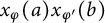 $x_{\varphi }(a)x_{\varphi '}(b)$
with
 $a,b\neq 0$
, and hence the “if” direction of the theorem follows from Theorems 4.1 and 5.4. Thus, it remains to prove the “only if” direction.
The result for the small building
 $\mathsf {E}_6(2)$
follows from [Reference Parkinson and Van Maldeghem16, Theorem 4.6]. Thus, suppose that
 $\Delta $
is large, and so the underlying field
 $\mathbb {F}$
has at least three elements. Note that
 $w_{\mathsf {A}_3}w_{\mathsf {E}_6}=s_{\varphi }s_{\varphi '}$
(by comparing inversion sets). Thus,
 $\operatorname {{\mathrm {disp}}}(\theta )=\ell (s_{\varphi }s_{\varphi '})$
, and because
 $\theta $
is capped,
 $\ell (\delta (gB,\theta gB))=\ell (s_{\varphi }s_{\varphi '})$
if and only if
 $\delta (gB,\theta gB)=s_{\varphi }s_{\varphi '}$
. Moreover, after replacing
 $\theta $
by a conjugate, we may assume that the base chamber B is mapped to Weyl distance
 $s_{\varphi }s_{\varphi '}$
(see [Reference Parkinson and Van Maldeghem15, Theorem 2.6]). Because the stabilizer of B is transitive on each w-sphere centered at B, we may assume that B is mapped to the chamber
 $x_{\varphi }(1)x_{\varphi '}(1)s_{\varphi }s_{\varphi '}B$
. By the folding relation, and the fact that
 $\varphi $
and
 $\varphi '$
are perpendicular, we have
 $x_{\varphi }(1)x_{\varphi '}(1)s_{\varphi }s_{\varphi '}B=x_{-\varphi }(1)x_{-\varphi '}(1)B$
. The condition
 $\theta (B)=x_{-\varphi }(1)x_{-\varphi '}(1)B$
gives
 $$ \begin{align*}\theta=x_{-\varphi}(1)x_{-\varphi'}(1)uh\sigma\quad\text{for some}\ u\in U^+, h\in H,\ \text{and}\ \sigma\in\mathrm{Aut}(\mathbb{F}). \end{align*} $$
We will now determine
 $u,h$
, and
 $\sigma $
. The primary strategy (as in Theorem 3.4) is to show that if these elements do not take certain particular forms, then one can find an element
 $g\in G$
such that
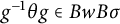 $g^{-1}\theta g\in BwB\sigma $
with
 $\ell (w)>\ell (s_{\varphi }s_{\varphi '})$
. Thus, the chamber
 $gB$
is mapped to distance
 $\ell (w)>\ell (s_{\varphi }s_{\varphi '})$
, contradicting the fact that
 $\theta $
has polar–copolar diagram. A useful observation is that if
 $w=s_{\varphi }s_{\varphi '}v$
with
 $v\in W_{\mathsf {A}_3}$
, then
 $\ell (w)=\ell (s_{\varphi }s_{\varphi '})+\ell (v)$
. We now proceed with the analysis. The first three steps are completely analogous to the proof of Theorem 3.4, and we omit the easy details.
Claim 1: We have
 $u\in U_{\Phi \backslash \Phi _1}^+$
.
Claim 2: We have
 $h=h_{\omega _1}(c_1)h_{\omega _2}(c_2)h_{\omega _6}(c_3)$
for some
 $c_1,c_2,c_3\in \mathbb {F}^{\times }$
.
Claim 3: We have
 $\sigma =\mathrm {id}$
.
Claim 4: We have
 $u\in U_{\varphi }U_{\varphi '}$
. Write
 $u=x_{\varphi }(c)x_{\varphi '}(d)u_1$
with
 $c,d\in \mathbb {F}$
and
 $u_1\in U_{\Phi \backslash (\Phi _1\cup \{\varphi ,\varphi '\})}^+$
. We must show that
 $u_1=1$
. Suppose not. Let
 $i\in \{1,2,3,4,5,6\}$
be minimal such that a root in
 $C_i$
appears in
 $u_1$
. Using the same idea as in the proof of Claim 4 in Theorem 3.4, one may then conjugate
 $u_1$
by an element
 $g\in U_{\Phi _1}^-$
to obtain
 $$ \begin{align*}g^{-1}u_1g=u_1^{\prime}x_{\beta_i+\varphi''}(b)x_{\beta_i}(a) \end{align*} $$
with
 $a\neq 0$
,
 $b\in \mathbb {F}$
, and
 $u_1^{\prime }$
a product of root elations with roots in
 $C_i^{\prime }$
. Moreover, because
 $g^{-1}hg=h$
(by Claim 2) and
 $g^{-1}x_{-\varphi }(1)x_{-\varphi '}(1)x_{\varphi }(c)x_{\varphi '}(d)g=x_{-\varphi }(1)x_{-\varphi '}(1)x_{\varphi }(c)x_{\varphi '}(d)$
(because
 $\pm \varphi -\alpha ,\pm \varphi '-\alpha \notin \Phi $
for all
 $\alpha \in \Phi _1^+$
), we have
 $$ \begin{align*}g^{-1}\theta g=x_{-\varphi}(1)x_{-\varphi^{\prime}}(1)x_{\varphi}(c)x_{\varphi^{\prime}}(d)u_1^{\prime}x_{\beta_i+\varphi^{\prime\prime}}(b)x_{\beta_i}(a)h. \end{align*} $$
Let
 $g_1=x_{-\beta _i-\varphi ''}(z)$
with
 $z\in \mathbb {F}$
. Then,
 $$ \begin{align*} g_1^{-1}g^{-1}\theta gg_1&=x_{-\beta_i-\varphi''}(-z)x_{-\varphi}(1)x_{-\varphi^{\prime}}(1)x_{\varphi}(c)x_{\varphi^{\prime}}(d)u_1^{\prime}x_{\beta_i+\varphi''}(b)\\ &\quad\times x_{\beta_i}(a)x_{-\beta_i-\varphi''}(\lambda z)h, \end{align*} $$
for some
 $\lambda \neq 0$
. Because
 $\Delta $
is large, we have
 $|\mathbb {F}|\geq 3$
, and so we may choose
 $z\in \mathbb {F}$
with
 $z\neq 0$
and
 $b\lambda z\neq -1$
. Applying Lemma 7.8 then gives
 $$ \begin{align*}g_1^{-1}g^{-1}\theta gg_1\in Bw_0s_4B, \end{align*} $$
and hence the chamber
 $g_1gB$
is mapped to Weyl distance
 $w_0s_4$
, a contradiction. Thus,
 $u_1=1$
.
Claim 5: We have
 $\theta =x_{-\varphi }(1)x_{-\varphi ^{\prime }}(1)x_{\varphi }(a)x_{\varphi ^{\prime }}(b)h_{\omega _1}(c_1)h_{\omega _2}(c_2)h_{\omega _6}(c_3)$
, where
 $$ \begin{align*} a=-(c_1c_2-1)(c_2c_3-1)\quad\text{and}\quad b=-(c_1-1)(c_3-1). \end{align*} $$
From Claims 1–4, we have
 $\theta =x_{-\varphi }(1)x_{-\varphi ^{\prime }}(1)x_{\varphi }(a)x_{\varphi ^{\prime }}(b)h_{\omega _1}(c_1)h_{\omega _2}(c_2)h_{\omega _6}(c_3)$
for some
 $a,b\in \mathbb {F}$
. Let
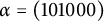 $\alpha =(101000)$
and
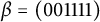 $\beta =(001111)$
, and let
 $g=x_{-\alpha }(1)x_{-\beta }(1)$
. A direct calculation shows that if
 $b\neq -(c_1-1)(c_3-1)$
, then
 $$ \begin{align*}g^{-1}\theta g\in Bs_{\varphi}s_{\varphi^{\prime}}B\cdot Bs_3B=Bs_{\varphi}s_{\varphi^{\prime}}s_3B, \end{align*} $$
a contradiction.
A similar calculation, with
 $g=x_{-\gamma }(1)x_{-\delta }(1)$
, where
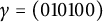 $\gamma =(010100)$
and
 $\delta =(112321)$
, shows that if
 $a\neq -(c_1c_2-1)(c_2c_3-1)$
, then
 $g^{-1}\theta g\in Bs_{\varphi }s_{\varphi ^{\prime }}s_4B$
, again a contradiction.
Claim 6:
 $\theta $
fixes a chamber. Let
 $gB=x_{\varphi }(y_1)x_{\varphi ^{\prime }}(y_2)s_{\varphi }s_{\varphi ^{\prime }}B$
with
 $y_1,y_2\in \mathbb {F}$
. With
 $\theta $
as in Claim 5, we have
 $$ \begin{align*} \theta gB&=x_{-\varphi}(1)x_{-\varphi^{\prime}}(1)x_{\varphi}(a)x_{\varphi^{\prime}}(b)x_{\varphi}(c_1c_2^2c_3y_1)x_{\varphi^{\prime}}(c_1c_3y_2)s_{\varphi}s_{\varphi^{\prime}}B\\ &=x_{-\varphi}(1)x_{\varphi}(a+c_1c_2^2c_3y_1)x_{-\varphi^{\prime}}(1)x_{\varphi^{\prime}}(b+c_1c_3y_2)s_{\varphi}s_{\varphi^{\prime}}B. \end{align*} $$
We now use the
 $\mathsf {SL}_2$
relation
 $x_{-\alpha }(z)x_{\alpha }(z^{\prime })=x_{\alpha }(z^{\prime }(1+zz^{\prime })^{-1})x_{-\alpha }(-z(1+zz^{\prime }))h_{\alpha ^{\vee }}(1+zz^{\prime })^{-1}$
, valid whenever
 $zz^{\prime }\neq -1$
, to obtain
 $$ \begin{align*} \theta gB&=x_{\varphi}((a+c_1c_2^2c_3y_1)(1+a+c_1c_2^2c_3y_1)^{-1})\\ &\quad \times x_{\varphi^{\prime}}((b+c_1c_3y_2)(1+b+c_1c_3y_2)^{-1})s_{\varphi}s_{\varphi^{\prime}}B, \end{align*} $$
where we have chosen
 $y_1,y_2$
, so that
 $1+a+c_1c_2^2c_3y_1\neq 0$
and
 $1+b+c_1c_3y_2\neq 0$
. We have
 $\theta gB=gB$
if and only if
 $(a+c_1c_2^2c_3y_1)=y_1(1+a+c_1c_2^2c_3y_1)$
and
 $(b+c_1c_3y_2)=y_2(1+b+c_1c_3y_2)$
. Recalling that
 $a=-(c_1c_2-1)(c_2c_3-1)$
and
 $b=-(c_1-1)(c_3-1)$
, the discriminants in the quadratics (in
 $y_1$
and
 $y_2$
) are perfect squares, and we find that
 $gB$
is fixed if and only if
 $$ \begin{align*} y_1&\in\{1-c_1^{-1}c_2^{-1},1-c_2^{-1}c_3^{-1}\}&y_2&\in\{1-c_1^{-1},1-c_3^{-1}\} \end{align*} $$
(note that these values avoid the excluded values
 $y_1=1-c_1^{-1}c_2^{-1}-c_2^{-1}c_3^{-1}$
and
 $y_2=1-c_1^{-1}-c_3^{-1}$
required for the
 $\mathsf {SL}_2$
relation to hold).
Claim 7:
 $\theta $
is conjugate to
 $x_{\varphi }(-c_1c_2)x_{\varphi ^{\prime }}(-c_1)h_{\omega _1}(c_1c_3^{-1})$
. Let
 $g=x_{\varphi }(1-c_1^{-1}c_2^{-1})x_{\varphi ^{\prime }}(1-c_1^{-1})s_{\varphi }s_{\varphi ^{\prime }}$
. It follows from Claim 5 that
 $g^{-1}\theta g\in B$
, and a direct calculation yields
 $$ \begin{align*} g^{-1}\theta g&=x_{\varphi}(-c_1c_2)x_{\varphi^{\prime}}(-c_1)h_{\omega_1}(c_1c_3^{-1}), \end{align*} $$
as required.
Claim 8:
 $\theta $
is either a product of perpendicular root elations, or a homology fixing a subbuilding with thick frame of type
 $\mathsf {D}_5$
. After conjugating, as in Claim 6, we may replace
 $\theta $
by the conjugate
 $\theta =x_{\varphi }(-c_1c_2)x_{\varphi ^{\prime }}(-c_1)h_{\omega _1}(c_1c_3^{-1})$
. If
 $c_1=c_3$
, then
 $\theta $
is a product of perpendicular root elations. If
 $c_1\neq c_3$
, then we note that the chamber
 $gB$
, with
 $g=x_{\varphi }(c_1c_2c_3/(c_1-c_3))x_{\varphi ^{\prime }}(c_1c_3/(c_1-c_3))s_{\varphi }s_{\varphi ^{\prime }}$
, is fixed by
 $\theta $
. Thus,
 $g^{-1}\theta g\in B$
, and a direct calculation shows that
 $$ \begin{align*}g^{-1}\theta g=h_{\omega_6}(c_1^{-1}c_3), \end{align*} $$
which is a homology fixing a subbuilding with thick frame of type
 $\mathsf {D}_5$
(by Theorem 5.4).▪
7.3 Classification of domestic automorphisms of split
$\mathsf {G}_2$
buildings

Let
 $\Phi $
be a root system of type
 $\mathsf {G}_2$
, with the convention that
 $\alpha _1$
is a short root. Note that
 $\alpha _2$
is the polar node. Let
 $\varphi =(32)$
be the highest root of
 $\Phi $
. The highest short root is
 $\varphi ^{\prime }=(21)$
. Let G be the Chevalley group
 $\mathsf {G}_2(\mathbb {F})$
. The building
 $\Delta =G/B$
may be regarded as a generalized hexagon (the dual split Cayley hexagon), where the point set is
 $G/P_1$
and the line set is
 $G/P_2$
, where
 $P_i=B\cup Bs_iB$
(in particular, note that “points” are type
 $\{2\}=S\backslash \{1\}$
vertices, and “lines” are type
 $\{1\}=S\backslash \{2\}$
vertices). Then,
 $G\rtimes \mathrm {Aut}(\mathbb {F})$
is the full collineation group of
 $\Delta $
.
Recall the following definitions. A distance
 $3$
-ovoid in a generalized hexagon
 $\mathscr {G}$
is a set
 $\mathcal {S}$
of mutually opposite points such that every element of the generalized hexagon is at distance at most
 $3$
(in the incidence graph) from a point of
 $\mathcal {S}$
. A subhexagon
 $\mathscr {G}^{\prime }$
of
 $\mathscr {G}$
is full if every point of
 $\mathscr {G}$
incident with a line of
 $\mathscr {G}^{\prime }$
belongs to
 $\mathscr {G}^{\prime }$
, and is large if every element of
 $\mathscr {G}$
is at distance at most
 $3$
from some element of
 $\mathscr {G}^{\prime }$
. Recall from [Reference Parkinson, Temmermans and Van Maldeghem14, Theorem 2.7] that a nontrivial automorphism
 $\theta $
of a generalized hexagon is point-domestic if and only if its fixed element structure is either a ball of radius
 $3$
in the incidence graph centered at a line, a large full subhexagon, or a distance
 $3$
-ovoid. Dual statements hold for line-domestic automorphisms. (Note that the “if” direction was omitted in the statement of [Reference Parkinson, Temmermans and Van Maldeghem14, Theorem 2.7]; however, it is obvious from fixed element structure in each case)
In this section, we prove the following theorem, which along with [Reference Parkinson, Temmermans and Van Maldeghem14, Theorems 2.7, 2.9, and 2.14] completely classifies the domestic automorphisms of
 $\Delta $
.
Theorem 7.10 Let
 $\Delta $
be the building of
 $\mathsf {G}_2(\mathbb {F})$
. There exists a unique conjugacy class
 $\mathscr {C}_1$
of automorphisms with opposition diagram
 $\mathsf {G}_{2;1}^2$
, and a unique conjugacy class
 $\mathscr {C}_2$
of automorphisms with opposition diagram
 $\mathsf {G}_{2;1}^1$
. The class
 $\mathscr {C}_1$
consists precisely of the long root elations. The class
 $\mathscr {C}_2$
has representative
 $\theta _2$
, where:
-
(1) if
$\mathrm {char}(\mathbb {F})=3$
, then
$\theta _2=x_{\varphi ^{\prime }}(1)$
is a short root elation fixing precisely a ball of radius
$3$
in the incidence graph centered at a line, -
(2) if there is
$z\in \mathbb {F}\backslash \{1\}$
with
$z^3=1$
, then
$\theta _2=h_{\omega _1}(z)$
is a homology fixing a large full subhexagon, and -
(3) if
$\mathrm {char}(\mathbb {F})\neq 3$
and there is no
$z\in \mathbb {F}\backslash \{1\}$
with
$z^3=1$
, then
$\theta _2=x_{\alpha _1}(1)s_1$
fixes precisely a distance
$3$
-ovoid.


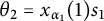

In particular, note that in the case (3), there is no automorphism fixing a chamber with opposition diagram
 $\mathsf {G}_{2;1}^1$
. This is the only case of a split building with this property. The proof of Theorem 7.10 will follow from a series of lemmas.
Lemma 7.11 Let
 $\Delta =\mathsf {G}_2(\mathbb {F})$
. A collineation
 $\theta $
fixes precisely a ball of radius
 $3$
in the incidence graph centered at a point (respectively a line) if and only if
 $\theta $
is conjugate to
 $x_{\varphi }(1)$
(respectively,
 $\mathrm {char}(\mathbb {F})=3$
and
 $\theta $
is conjugate to
 $x_{\varphi ^{\prime }}(1)$
). Moreover, the automorphism
 $x_{\varphi }(1)$
is domestic with opposition diagram
 $\mathsf {G}_{2;1}^2$
, and the automorphism
 $x_{\varphi ^{\prime }}(1)$
is domestic if and only if
 $\mathrm {char}(\mathbb {F})=3$
, in which case it has opposition diagram
 $\mathsf {G}_{2;1}^1$
.
Proof Consider the case where the center is a line L, and let p be a point on L. Then,
 $\{p,L\}$
is a chamber fixed by
 $\theta $
, and after conjugation, we may suppose that
 $\{p,L\}$
is the base chamber B. Because
 $\theta $
fixes all points on the line L, it follows that
 $\theta $
is linear, and hence
 $\theta \in \mathsf {G}_2(\mathbb {F})$
. In the
 $BN$
-pair language, the hypothesis of the lemma gives that
 $\theta $
fixes each chamber
 $gB$
with
 $g\in B\cup Bs_1B\cup Bs_2B\cup Bs_1s_2B\cup Bs_2s_1B\cup Bs_2s_1s_2B$
. In particular,
 $\theta (B)=B$
, and so
 $\theta \in B$
. Thus,
 $\theta =hu$
with
 $h=h_{\omega _1}(c_1)h_{\omega _2}(c_2)\in H$
and
 $u\in U^+$
. Write
 $$ \begin{align*}u=x_{10}(a_1)x_{01}(a_2)x_{11}(a_3)x_{21}(a_4)x_{31}(a_5)x_{32}(a_6). \end{align*} $$
By commutator relations and the fact that
 $s_1(\alpha )\in \Phi ^+$
for all
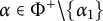 $\alpha \in \Phi ^+\backslash \{\alpha _1\}$
, we have
 $$ \begin{align*}\theta x_{\alpha_1}(a)s_1B=x_{\alpha_1}((a+a_1)c_1)s_1B, \end{align*} $$
and because
 $\theta $
fixes each chamber
 $x_{\alpha _1}(a)s_1B$
with
 $a\in \mathbb {F}$
, we have
 $a_1=0$
and
 $c_1=1$
. Similarly, because
 $\theta x_{\alpha _2}(a)s_2B=x_{\alpha _2}((a+a_2)c_2)s_2B$
, we have
 $a_2=0$
and
 $c_2=1$
. Thus,
 $h=1$
. Next, because
 $\theta $
fixes each chamber
 $x_{10}(a)s_1s_2B$
with
 $a\in \mathbb {F}$
, we have
 $$ \begin{align*} x_{31}(a)s_1s_2B&=\theta x_{31}(a)s_1s_2B=x_{31}(a+a_5)s_1s_2B, \end{align*} $$
and so
 $a_5=0$
. Similarly, because the chamber
 $x_{11}(a)s_2s_1B$
is fixed for all
 $a\in \mathbb {F}$
, we have
 $a_3=0$
. Next, the condition that
 $x_{32}(a)s_2s_1s_2B$
is fixed for all
 $a\in \mathbb {F}$
yields
 $a_6=0$
, and so
 $\theta =x_{\varphi ^{\prime }}(a_4)$
. However, in addition, the chamber
 $x_{11}(a)s_2s_1s_2B$
must be fixed, and a calculation gives
 $$ \begin{align*}\theta x_{11}(a)s_2s_1s_2B=x_{11}(a)x_{32}(3a_4a)s_2s_1s_2B. \end{align*} $$
Thus,
 $\mathrm {char}(\mathbb {F})=3$
. We may then conjugate
 $h_{\omega _2}(a_4^{-1})\theta h_{\omega _2}(a_4)=x_{\varphi ^{\prime }}(1)$
, and the result now follows in this case by Theorem 3.10.
In the case that the center is a point, a very similar analysis to the above gives
 $\theta =x_{\varphi }(a)$
for some
 $a\neq 0$
, and this element is conjugate to
 $x_{\varphi }(1)$
. Because this element is central in
 $U^+$
, it is clear that
 $\theta $
does indeed fix a ball of radius
 $3$
, and moreover, by Theorem 3.1, it has opposition diagram
 $\mathsf {G}_{2,1}^2$
.▪
Lemma 7.12 There exists a collineation of
 $\Delta $
fixing precisely a distance
 $3$
-ovoid if and only if the polynomial
 $z^2+z+1$
is irreducible over
 $\mathbb {F}$
. Moreover, if
 $z^2+z+1$
is irreducible over
 $\mathbb {F}$
, then there is a unique conjugacy class of collineations fixing an ovoid, with representative
 $\theta =x_{\alpha _1}(1)s_1$
.
Proof Suppose that
 $\theta $
fixes a distance
 $3$
-ovoid (and hence is point-domestic). Because the automorphism group of
 $\Delta $
is transitive on pairs of opposite vertices, we may assume that the points
 $P_1$
and
 $w_0P_1$
are both fixed. Write
 $\theta =\theta _0\cdot \sigma $
, with
 $\theta \in G$
and
 $\sigma \in \mathrm {Aut}(\mathbb {F})$
. We have
 $\theta P_1=\theta _0 P_1$
, and so
 $\theta _0\in P_1=B\cup Bs_1B$
. If
 $\theta _0\in B$
, then
 $\theta $
fixes the chamber B, a contradiction. Thus,
 $\theta _0\in Bs_1B$
. Each element of
 $Bs_1B$
can be written as
 $x_{\alpha _1}(a)s_1b$
with
 $b\in B$
. Replacing
 $\theta $
by the conjugate
 $b^{\sigma }\theta b^{-\sigma }$
, we may write
 $$ \begin{align*}\theta=hu_1x_{\alpha_1}(a)s_1\cdot\sigma, \end{align*} $$
where
 $h=h_{\omega _1}(c_1)h_{\omega _2}(c_2)$
with
 $c_1,c_2\in \mathbb {F}^{\times }$
,
 $u_1\in \prod _{\alpha \in \Phi ^+\backslash \{\alpha _1\}}U_{\alpha }$
, and
 $a\in \mathbb {F}$
.
Claim 1:
 $u_1=1$
. Because
 $\theta $
fixes
 $w_0P_1$
, and because
 $\sigma $
fixes
 $w_0$
, we have
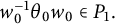 $ w_0^{-1}\theta _0 w_0\in P_1. $
However,
 $$ \begin{align*} w_0^{-1}\theta_0w_0&=(w_0^{-1}hw_0)(w_0^{-1}u_1w_0)(w_0^{-1}x_{\alpha_1}(a)s_1w_0), \end{align*} $$
and because the first and third grouped terms are in
 $P_1$
, we have
 $w_0^{-1}u_1w_0\in P_1=B\cup Bs_1B$
. If
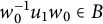 $w_0^{-1}u_1w_0\in B$
, then because
 $w_0^{-1}u_1w_0$
is also in the opposite Borel, we have
 $u_1\in H$
, and so
 $u_1=1$
. If
 $w_0^{-1}u_1w_0\in Bs_1B$
, then
 $u_1w_0\in w_0Bs_1B=U^-w_0s_1B=U^-s_2s_1s_2s_1s_2B$
. However, writing
 $$ \begin{align*}u_1w_0B=x_{10}(0)x_{31}(d_1)x_{21}(d_2)x_{32}(d_3)x_{11}(d_4)x_{01}(d_5)s_1s_2s_1s_2s_1s_2B, \end{align*} $$
the folding algorithm described in [Reference Parkinson, Ram and Schwer13, Section 7] implies that:
-
–if
$d_1\neq 0$
, then
$u_1w_0B\subseteq U^-vB$
for some
$v\in \{1,s_1,s_2,s_1s_2,s_2s_1,s_2s_1s_2\}$
; -
–if
$d_1= 0$
and
$d_2\neq 0$
, then
$u_1w_0B\subseteq U^-s_2B$
; -
–if
$d_1=d_2=0$
and
$d_3\neq 0$
, then
$u_1w_0B\subseteq U^-s_1B$
; -
–if
$d_1=d_2=d_3=0$
and
$d_4\neq 0$
, then
$u_1w_0B\subseteq U^-s_1s_2s_1B$
; -
–if
$d_1=d_2=d_3=d_4=0$
and
$d_5\neq 0$
, then
$u_1w_0B\subseteq U^-s_1s_2s_1s_2s_1B$
.















This contradiction shows that indeed
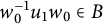 $w_0^{-1}u_1w_0\in B$
, and hence
 $u_1=1$
.
Claim 2:
 $c_1^3c_2^2=1$
and
 $\sigma =1$
. We have
 $\theta =hx_{\alpha _1}(a)s_1\cdot \sigma $
, where
 $h=h_{\omega _1}(c_1)h_{\omega _2}(c_2)$
. Consider the chamber
 $x_{\varphi }(z)w_0B$
, where
 $z\in \mathbb {F}$
. We have
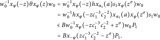 $$ \begin{align*} w_0^{-1}x_{\varphi}(-z)\theta x_{\varphi}(z)w_0&=w_0^{-1}x_{\varphi}(-z)hx_{\alpha_1}(a)s_1x_{\varphi}(z^{\sigma})w_0\\ &=w_0^{-1}hx_{\varphi}(-zc_1^{-3}c_2^{-2})x_{\alpha_1}(a)x_{\varphi}(z^{\sigma})s_1w_0\\ &\in Bw_0^{-1}x_{\varphi}(-zc_1^{-3}c_2^{-2}+z^{\sigma})w_0P_1\\ &=Bx_{-\varphi}(zc_1^{-3}c_2^{-2}-z^{\sigma})P_1. \end{align*} $$
If
 $zc_1^{-3}c_2^{-2}-z^{\sigma }\neq 0$
, then
 $w_0^{-1}x_{\varphi }(-z)\theta x_{\varphi }(z)w_0\in Bs_{\varphi }P_1$
, and because
 $s_{\varphi }=s_2s_1s_2s_1s_2$
, it follows that the point of the chamber
 $x_{\varphi }(z)w_0B$
is mapped to an opposite point, a contradiction. Thus,
 $zc_1^{-3}c_2^{-2}-z^{\sigma }=0$
for all
 $z\in \mathbb {F}$
. The case
 $z=1$
gives
 $c_1^3c_2^2=1$
, and then the equation reads
 $z-z^{\sigma }=0$
, and so
 $\sigma $
is trivial.
Claim 3: We may assume that either
 $a=0$
or
 $a=1$
. Suppose that
 $a\neq 0$
. Then, because
 $s_1(\omega _1)=-\omega _1+3\omega _2$
, we have
 $$ \begin{align*} h_{\omega_1}(a)^{-1}\theta h_{\omega_1}(a)&=h_{\omega_1}(a^{-1}c_1)h_{\omega_2}(c_2)x_{\alpha_1}(a)h_{-\omega_1+3\omega_2}(a)s_1\\ &=h_{\omega_1}(a^{-1}c_1)h_{\omega_2}(c_2)h_{-\omega_1+3\omega_2}(a)x_{\alpha_1}(1)s_1\\ &=h_{\omega_1}(a^{-2}c_1)h_{\omega_2}(a^3c_2)x_{\alpha_1}(1)s_1. \end{align*} $$
Renaming
 $a^{-2}c_1$
and
 $a^3c_2$
by
 $c_1$
and
 $c_2$
gives the result.
Claim 4: We have
 $\mathrm {char}(\mathbb {F})\neq 3$
. Suppose that
 $\mathrm {char}(\mathbb {F})=3$
. Suppose first that
 $a=0$
. Then, a calculation shows that the point
 $ x_{01}(1)x_{31}(1)s_2s_1s_2s_1s_2P_1 $
is mapped to the point
 $x_{01}(-c_2)x_{32}(1)x_{31}(c_2^{-1})s_2s_1s_2s_1s_2P_1$
, and that these points are opposite, a contradiction.
Now, suppose that
 $a=1$
. Because
 $c_1^3c_2^2=1$
, we have
 $h_{\omega _1}(c_1)h_{\omega _2}(c_2)=h_{\alpha _1^{\vee }}(c)$
, where
 $c=c_1^{-1}c_2^{-1}$
. Thus,
 $\theta =h_{\alpha _1^{\vee }}(c)x_{10}(1)s_1$
. Now, writing
 $u=x_{01}(c^{-3})x_{11}(-c^{-1})x_{21}(1)x_{31}(-1)$
, if
 $c\neq 1$
, we calculate
 $$ \begin{align*}P_1w_0^{-1}u^{-1}\theta uw_0P_1=P_1s_2s_1s_2s_1s_2P_1, \end{align*} $$
showing that the point
 $uw_0P_1$
is mapped to an opposite point, a contradiction. Thus,
 $c=1$
, and hence
 $c_1=c_2=1$
. But then,
 $$ \begin{align*} \theta=x_{10}(1)s_1=x_{10}(2)x_{-10}(-1)x_{10}(1)=x_{10}(-1)x_{-10}(-1)x_{10}(1), \end{align*} $$
and hence
 $\theta $
is conjugate to a root elation, a contradiction.
Claim 5: We have
 $a\neq 0$
and
 $c_1=c_2=1$
. Recall that
 $\theta =hx_{\alpha _1}(a)s_1$
, with
 $h_{\omega _1}(c_1)h_{\omega _2}(c_2)$
, where
 $c_1^3c_2^2=1$
, and
 $a\in \{0,1\}$
. Consider the chamber
 $gB$
where
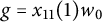 $g=x_{11}(1)w_0$
. Then,
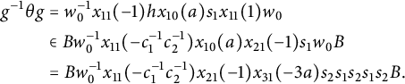 $$ \begin{align*} g^{-1}\theta g&=w_0^{-1}x_{11}(-1)hx_{10}(a)s_1x_{11}(1)w_0\\ &\in Bw_0^{-1}x_{11}(-c_1^{-1}c_2^{-1})x_{10}(a)x_{21}(-1)s_1w_0B\\ &=Bw_0^{-1}x_{11}(-c_1^{-1}c_2^{-1})x_{21}(-1)x_{31}(-3a)s_2s_1s_2s_1s_2B. \end{align*} $$
Write
 $u=x_{11}(-c_1^{-1}c_2^{-1})x_{21}(-1)x_{31}(-3a)$
. We will show below that if either
 $a= 0$
or
 $c_1c_2\neq 1$
, then
 $ us_2s_1s_2s_1s_2B\subseteq U^-B=w_0Bw_0B, $
which in turn gives
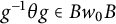 $g^{-1}\theta g\in Bw_0B$
, a contradiction with point-domesticity. To prove the above statement, we compute
 $$ \begin{align*} us_2s_1s_2s_1s_2B&=x_{-11}(-c_1c_2)x_{11}(c_1^{-1}c_2^{-1})n_{11}(-c_1^{-1}c_2^{-1})x_{21}(-1)x_{31}(-3a)s_2s_1s_2s_1s_2B\\ &\subseteq U^-x_{11}(c_1^{-1}c_2^{-1})x_{10}(-c_1c_2)x_{31}(-3a)s_1s_2B. \end{align*} $$
Commutator relations give
 $$ \begin{align*} &x_{11}(c_1^{-1}c_2^{-1})x_{10}(-c_1c_2)x_{31}(-3a)\\ &\quad=x_{10}(-c_1c_2)x_{31}(3(c_1c_2-a))x_{11}(c_1^{-1}c_2^{-1})x_{32}(3c_1^{-1}c_2^{-1})x_{21}(2). \end{align*} $$
Using this in the above equation, and noting that the final three terms can pass past the
 $s_1s_2$
and remain in B, we have
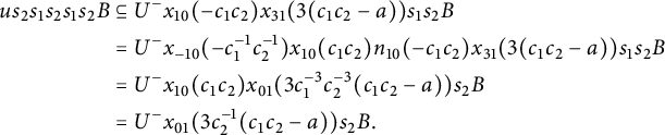 $$ \begin{align*} us_2s_1s_2s_1s_2B&\subseteq U^-x_{10}(-c_1c_2)x_{31}(3(c_1c_2-a))s_1s_2B\\ &=U^-x_{-10}(-c_1^{-1}c_2^{-1})x_{10}(c_1c_2)n_{10}(-c_1c_2)x_{31}(3(c_1c_2-a))s_1s_2B\\ &=U^-x_{10}(c_1c_2)x_{01}(3c_1^{-3}c_2^{-3}(c_1c_2-a))s_2B\\ &=U^-x_{01}(3c_2^{-1}(c_1c_2-a))s_2B. \end{align*} $$
Recall that
 $\mathrm {char}(\mathbb {F})\neq 3$
. Thus, if either
 $a=0$
, or
 $a=1$
and
 $c_1c_2\neq 1$
, we have
 $us_2s_1s_2s_1s_2B\subseteq U^-B$
as required.
Claim 6: The polynomial
 $z^2+z+1$
is irreducible over
 $\mathbb {F}$
. Because
 $\theta $
fixes no lines, in particular, no line through
 $P_1$
is fixed. Equivalently, none of the chambers B and
 $x_{\alpha _1}(-z)s_1B$
with
 $z\in \mathbb {F}$
are fixed by
 $\theta $
. Clearly, B is not fixed, and for
 $z\neq 0$
, we have
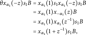 $$ \begin{align*} \theta x_{\alpha_1}(-z)s_1B&=x_{\alpha_1}(1)s_1x_{\alpha_1}(-z)s_1B\\[-1pt] &=x_{\alpha_1}(1)x_{-\alpha_1}(z)B\\[-1pt] &=x_{\alpha_1}(1)x_{\alpha_1}(z^{-1})s_1B\\[-1pt] &=x_{\alpha_1}(1+z^{-1})s_1B, \end{align*} $$
and so
 $1+z^{-1}\neq -z$
for all
 $z\in \mathbb {F}^{\times }$
. Hence the claim.
So far, we have proved that if
 $\theta $
fixes a distance
 $3$
-ovoid, then
 $\theta $
is conjugate to
 $x_{\alpha _1}(1)s_1$
and the polynomial
 $z^2+z+1=0$
is irreducible over
 $\mathbb {F}$
. It remains to show that if this polynomial is irreducible, then the element
 $\theta =x_{\alpha _1}(1)s_1$
does indeed fix a distance
 $3$
-ovoid. We have shown that no line through the fixed point
 $P_1$
is fixed. This implies that the fixed element structure of
 $\theta $
consists of a set of mutually opposite points (for otherwise by projecting onto
 $P_1$
gives a fixed line through
 $P_1$
). Thus, it is sufficient to prove point-domesticity to deduce that the fixed structure is a distance
 $3$
-ovoid.
By Lemma 2.6, it is sufficient to show that no point opposite the base point is mapped onto an opposite point. These points are of the form
 $$ \begin{align*}gs_2s_1s_2s_1s_2P_1=x_{01}(a_1)x_{11}(a_2)x_{32}(a_3)x_{21}(a_4)x_{31}(a_5)s_2s_1s_2s_1s_2P_1. \end{align*} $$
We compute
 $$ \begin{align*}g^{-1}\theta g=x_{01}(a^{\prime})x_{11}(b^{\prime})x_{21}(b^{\prime})x_{31}(3b^{\prime}-a^{\prime})x_{10}(1)s_1, \end{align*} $$
where
 $a^{\prime }=-a_1-a_5$
and
 $b^{\prime }=-a_2+a_4-a_5$
, and hence
 $$ \begin{align*} P_1s_{\varphi}^{-1}g^{-1}\theta g s_{\varphi}P_1&=P_1x_{-31}(-a^{\prime})x_{-21}(b^{\prime})x_{-11}(-b^{\prime})x_{-01}(3b^{\prime}-a^{\prime})P_1. \end{align*} $$
The folding algorithm then easily gives
 $$ \begin{align*} P_1s_{\varphi}^{-1}g^{-1}\theta g s_{\varphi}P_1&\in\begin{cases} P_1&\text{if}\ a^{\prime}=b^{\prime}=0\\ P_1s_2s_1s_2P_1&\text{otherwise,} \end{cases} \end{align*} $$
completing the proof.▪
Lemma 7.13 There exists a collineation of
 $\Delta $
fixing precisely a large full subhexagon if and only if the equation
 $z^2+z+1$
has a solution
 $z\neq 1$
in
 $\mathbb {F}$
. Moreover, if
 $z^2+z+1=0$
with
 $z\neq 1$
, then there is a unique conjugacy class of collineations fixing a large full subhexagon, with representative
 $\theta =h_{\omega _1}(z)$
.
Proof We may, after conjugating, suppose that the base apartment is fixed. Moreover, as the fixed subhexagon is full, all points on a line are fixed, and so
 $\theta $
is linear. Thus,
 $\theta =h_{\omega _1}(c_1)h_{\omega _2}(c_2)\in H$
. But fullness means that all points on the line
 $L=P_2$
are fixed. These points are
 $P_1$
and
 $x_{\alpha _2}(a)s_2P_1$
for
 $a\in \mathbb {F}$
. Because
 $$ \begin{align*}\theta x_{\alpha_2}(a)s_2P_1=x_{\alpha_1}(ac_2)s_2P_1, \end{align*} $$
we have
 $c_2=1$
. Thus,
 $\theta =h_{\omega _1}(c)$
for some
 $c\in \mathbb {F}^{\times }$
. Consider the chamber
 $gB=x_{\varphi }(1)w_0B$
. Then,
 $$ \begin{align*}Bg^{-1}\theta gB=Bw_0^{-1}x_{\varphi}(c^3-1)w_0^{-1}B. \end{align*} $$
If
 $c^3-1\neq 0$
, then this double coset is
 $Bs_{\varphi }B=Bs_2s_1s_2s_1s_2B$
, which means that the point of this chamber is mapped to an opposite point, a contradiction. So
 $c^3-1=0$
. If
 $c=1$
, then
 $\theta $
is the identity, a contradiction (as
 $\theta $
maps a line to an opposite line). So
 $c^2+c+1=0$
has a solution
 $c\neq 1$
(in particular,
 $\mathrm {char}(\mathbb {F})\neq 3$
). Finally, we show that in this case, the automorphism
 $\theta =h_{\omega _1}(c)$
does indeed have opposition diagram
 $\mathsf {G}_{2;1}^1$
. It suffices to show that no point opposite the base point
 $P_1$
is mapped to an opposite point. Each such point is of the form
 $us_{\varphi }P_1$
, where
 $$ \begin{align*}u=x_{01}(a_1)x_{11}(a_2)x_{32}(a_3)x_{21}(a_4)x_{31}(a_5). \end{align*} $$
Commutator relations, and the fact that
 $c^3=1$
, imply that
 $$ \begin{align*} u^{-1}\theta u &=x_{11}(a_2(c-1))x_{32}(3a_2a_4(1-c))x_{21}(a_4(c^2-1))h_{\omega_1}(c). \end{align*} $$
Thus,
 $$ \begin{align*} P_1s_{\varphi}^{-1}u^{-1}\theta us_{\varphi}P_1&=P_1x_{-21}(a_2(c-1))x_{-32}(3a_2a_4(c-1))x_{-11}(a_4(1-c^2))P_1. \end{align*} $$
Explicit computation then shows that
 $P_1s_{\varphi }^{-1}u^{-1}\theta us_{\varphi }P_1\in P_1\cup P_1s_2s_1s_2P_1$
, completing the proof.▪
We now give the proof of Theorem 7.10.
Proof of Theorem 7.10. An automorphism with opposition diagram
 $\mathsf {G}_{2,1}^1$
must fix either a ball of radius
 $3$
centered at a line, a large full subhexagon, or a distance
 $3$
-ovoid, and the result follows from Lemmas 7.11–7.13.
Consider the opposition diagram
 $\mathsf {G}_{2,1}^2$
. The fixed element structure of an automorphism with this diagram is necessarily either a ball of radius
 $3$
centered at a point, a large ideal subhexagon (where ideal is the dual notion to full), or a distance
 $3$
-spread (the dual notion to a distance
 $3$
-ovoid).
Large ideal subhexagons do not exist in the dual split Cayley hexagon, by [Reference Van Maldeghem30, Remark 5.9.14]. Suppose that
 $\theta $
fixes a distance
 $3$
-spread. We argue as in the proof of Lemma 7.12. As in that proof, we have
 $\theta =hu_1x_{\alpha _2}(a)s_2\cdot \sigma $
, where
 $h=h_{\omega _1}(c_1)h_{\omega _2}(c_2)$
with
 $c_1,c_2\in \mathbb {F}^{\times }$
,
 $u_1\in \prod _{\alpha \in \Phi ^+\backslash \{\alpha _2\}}U_{\alpha }$
, and
 $a\in \mathbb {F}$
. The proof of Claim 1 of Lemma 7.12 holds in an analogous fashion, yielding
 $u_1=1$
. Following the argument of Claim 2, considering the chamber
 $gB=x_{\varphi '}(z)w_0B$
, we have
 $$ \begin{align*}w_0^{-1}x_{\varphi'}(-z)\theta x_{\varphi'}(z)w_0\in Bx_{-\varphi'}(zc_1^{-2}c_1^{-1}-z^{\sigma})P_2, \end{align*} $$
from which it follows that
 $zc_1^{-2}c_1^{-1}-z^{\sigma }=0$
for all
 $z\in \mathbb {F}$
. Setting
 $z=1$
gives
 $c_1^2c_2=1$
, and then the equation reads
 $z-z^{\sigma }=0$
, and so
 $\sigma $
is trivial. Thus,
 $\theta =h_{\omega _1}(c)h_{\omega _2}(c^{-2})x_{\alpha _2}(a)s_2$
for some
 $c\in \mathbb {F}^{\times }$
and
 $a\in \mathbb {F}$
. We may assume that either
 $a=0$
, or
 $a=1$
(by conjugating by
 $h_{\omega _2}(c^2a^{-1})$
). If
 $a=0$
, with
 $\mathrm {char}(\mathbb {F})\neq 2$
, we see that the chamber
 $x_{10}(1)s_1s_2s_1B$
is mapped to an opposite. If
 $a=1$
with
 $\mathrm {char}(\mathbb {F})\neq 2$
, we see that if
 $c\neq -1/2$
, then
 $x_{10}(1)s_1s_2s_1B$
is mapped to an opposite, and if
 $c=-1/2$
, then
 $x_{10}(1)x_{11}(1)s_1s_2s_1B$
is mapped to an opposite. If
 $\mathrm {char}(\mathbb {F})=2$
and
 $a=1$
, then the chamber
 $x_{10}(1)s_1s_2s_1B$
is mapped onto an opposite chamber.
Suppose
 $\mathrm {char}(\mathbb {F})=2$
and that
 $a=0$
. Because no chamber is fixed, we compute (for
 $z\neq 0$
)
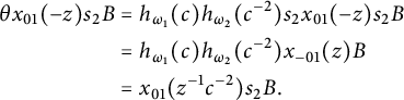 $$ \begin{align*} \theta x_{01}(-z)s_2B&=h_{\omega_1}(c)h_{\omega_2}(c^{-2})s_2x_{01}(-z)s_2B\\ &=h_{\omega_1}(c)h_{\omega_2}(c^{-2})x_{-01}(z)B\\ &=x_{01}(z^{-1}c^{-2})s_2B. \end{align*} $$
Thus,
 $z^{-1}c^{-2}\neq -z$
, and so
 $z^2\neq -c^{-2}$
for all
 $z\neq 0$
. This is a contradiction (taking
 $z=c^{-1}$
and recalling that
 $\mathrm {char}(\mathbb {F})=2$
).▪
We note that Corollary 10 follows from the above results:
Proof of Corollary 10. The polar closed admissible diagrams are realized as the opposition diagrams of unipotent elements, by Theorem 5. The admissible diagram
 $\mathsf {F}_{4;1}^4$
is achieved as the opposition diagram of either the homology
 $h_{\omega _4}(-1)$
(if
 $\mathrm {char}(\mathbb {F})\neq 2$
) or the short root elation
 $x_{\varphi '}(1)$
(in the case
 $\mathrm {char}(\mathbb {F})=2$
) by Lemma 5.8 and Corollary 7.7. All of these automorphisms lie in B, and hence fix the base chamber of
 $\Delta =G/B$
. The remaining diagram is
 $\mathsf {G}_{2;1}^1$
, and the result follows from Theorem 7.10.▪
7.4 Group theoretic consequences
We conclude with group theoretic applications of our results, proving Corollaries 11 and 12 from the introduction, and providing some further similar applications.
The proof of Corollary 11 is as follows.
Proof of Corollary 11. Let
 $\mathscr {C}$
be a conjugacy class in G. Suppose that
 $\mathscr {C}\cap Bw_0B=\emptyset $
. Then, no chamber is mapped onto an opposite chamber by any element of
 $\mathscr {C}$
(for if
 $\theta \cdot gB$
is opposite
 $gB$
, then
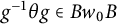 $g^{-1}\theta g\in Bw_0B$
). Thus, every element of
 $\mathscr {C}$
is domestic. By Theorems 3.4, 6.1, and 7.1, every domestic automorphism of a large building of type
 $\mathsf {E}_6$
or
 $\mathsf {F}_4$
necessarily fixes a chamber, and hence
 $\mathscr {C}\cap B\neq \emptyset $
. Similarly, for the small buildings of type
 $\mathsf {E}_6$
or
 $\mathsf {F}_4$
, every domestic automorphism fixes a chamber by [Reference Parkinson and Van Maldeghem16, Theorems 4.4 and 4.6], and hence the result.▪
The proof of Corollary 12 is as follows.
Proof of Corollary 12. By Corollary 2, every Moufang spherical building, with the exception of a projective plane, admits a type preserving domestic automorphism (a long root elation). The conjugacy class of such an automorphism thus intersects trivially with
 $Bw_0B$
.▪
It follows, from Remark 7.16 below, that the statement of Corollary 11 fails in general for buildings of types
 $\mathsf {E}_7$
and
 $\mathsf {E}_8$
(as there exist domestic automorphisms fixing no chamber). In these cases, we have the following results.
Corollary 7.14 Let
 $G=G_{\Phi }(\mathbb {F})$
be a Chevalley group of type
 $\mathsf {E}_7$
with
 $|\mathbb {F}|>2$
. Let
 $\varphi _1$
(respectively
 $\varphi _2,\varphi _3$
) be the highest root of the
 $\mathsf {E}_7$
(respectively
 $\mathsf {D}_6$
,
 $\mathsf {D}_4$
) subsystem. For each nontrivial conjugacy class
 $\mathscr {C}$
in G, we have both
 $$ \begin{align*} &\mathscr{C}\cap (Bs_{\varphi_1}B\cup Bs_{\varphi_1}s_{\varphi_2}B\cup Bs_{\varphi_1}s_{\varphi_2}s_7B\cup Bs_{\varphi_1}s_{\varphi_2}s_{\varphi_3}s_3B\cup Bw_0B)\neq \emptyset,\text{ and}\\ &\mathscr{C}\cap(B\cup Bs_{\varphi_1}s_{\varphi_2}s_7B\cup Bs_{\varphi_1}s_{\varphi_2}s_{\varphi_3}s_3B\cup Bw_0B)\neq \emptyset. \end{align*} $$
Proof If
 $\mathscr {C}$
is a nontrivial conjugacy class, then every element of
 $\mathscr {C}$
has nonempty opposition diagram. Let
 $\theta \in \mathscr {C}$
. If
 $J=\operatorname {{\mathrm {Typ}}}(\theta )$
, then by [Reference Parkinson and Van Maldeghem15, Theorem 2.6], there is a chamber
 $gB$
with
 $\delta (gB,\theta \cdot gB)=w_{S\backslash J}w_0$
, and so
 $g^{-1}\theta g\in Bw_{S\backslash J}w_0B$
. Hence,
 $\mathscr {C}\cap Bw_{S\backslash J}w_0B\neq \emptyset $
. The first statement then follows from the classification of admissible diagrams. The second statement follows from the fact that, by Theorem 6.1, every automorphism with opposition diagram either
 $\mathsf {E}_{7;2}$
or
 $\mathsf {E}_{8;2}$
necessarily fixes a chamber, and hence is conjugate to an element of B.▪
In the case
 $\mathbb {F}=\mathbb {F}_2$
, there exist uncapped automorphisms, and some additional double cosets need to be included in the statement of Corollary 7.14.
Corollary 7.15 Let
 $G=G_{\Phi }(\mathbb {F})$
be a Chevalley group of type
 $\mathsf {E}_8$
with
 $|\mathbb {F}|>2$
. Let
 $\varphi _1$
(respectively
 $\varphi _2,\varphi _3$
) be the highest root of the
 $\mathsf {E}_8$
(respectively
 $\mathsf {E}_7$
,
 $\mathsf {D}_6$
) subsystem. For each nontrivial conjugacy class
 $\mathscr {C}$
in G, we have both
 $$ \begin{align*} &\mathscr{C}\cap (Bs_{\varphi_1}B\cup Bs_{\varphi_1}s_{\varphi_2}B\cup Bs_{\varphi_1}s_{\varphi_2}s_{\varphi_3}s_7B\cup Bw_0B)\neq \emptyset,\text{ and}\\ &\mathscr{C}\cap(B\cup Bs_{\varphi_1}s_{\varphi_2}s_{\varphi_3}s_7B\cup Bw_0B)\neq \emptyset. \end{align*} $$
Proof The proof is similar to Corollary 7.14.▪
We conclude with the following remark.
Remark 7.16 The results of this paper (along with [Reference Van Maldeghem and Sastry32]) completely classify the automorphisms of split spherical buildings of exceptional type with opposition diagrams other than
 $\mathsf {E}_{7;3}$
,
 $\mathsf {E}_{7;4}$
, and
 $\mathsf {E}_{8;4}$
(with the possible exception of polar–copolar diagrams for small
 $\mathsf {E}_7$
and
 $\mathsf {E}_8$
buildings). For these three excluded diagrams, we have provided examples (both unipotent elements and homologies) with the respective opposition diagram, and the general classification for these diagrams will be continued in [Reference Parkinson, Van Maldeghem and Victoor18]. For now, we simply state, without proof, that in both
 $\mathsf {E}_7$
and
 $\mathsf {E}_8$
, the element
 $\theta =x_{\alpha _1}(1)s_1$
has order
 $3$
and opposition diagram
 $\mathsf {E}_{7;4}$
or
 $\mathsf {E}_{8;4}$
(for all fields). Thus, for example, if
 $\mathbb {F}=\mathbb {F}_2$
, then
 $\theta $
necessarily does not fix a chamber (as the Borel is a Sylow
 $2$
-group in this case), and hence is neither in
 $U^+$
nor in H. Furthermore, for type
 $\mathsf {E}_7$
, the element
 $\theta =x_{\alpha _2}(1)s_2x_{\alpha _5}(1)s_5x_{\alpha _7}(1)s_7$
has order
 $3$
and opposition diagram
 $\mathsf {E}_{7;3}$
, and similar statements apply.
Appendix A Root system data
The following table lists the number of positive roots (equivalently, the length of the longest element), the highest root
 $\varphi $
, the highest short root
 $\varphi '$
, the polar type
 $\wp $
, the dual polar type
 $\wp '$
, and the copolar type
 $\wp ^*$
for each irreducible crystallographic root system. Note that the copolar type is not well defined in the
 $\mathsf {B}_n$
and
 $\mathsf {D}_n$
cases as
 $S\backslash \wp $
is not irreducible.
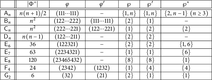 $$ \begin{align*}{ \begin{array}{|c||c|c|c|c|c|c|} \hline &|\Phi^+|&\varphi&\varphi'&\wp&\wp'&\wp^*\\ \hline\hline \mathsf{A}_n&n(n+1)/2&(111\cdots111)&-&\{1,n\}&\{1,n\}&\{2,n-1\}\,\,(n\geq 3)\\ \hline \mathsf{B}_n&n^2&(122\cdots222)&(111\cdots111)&\{2\}&\{1\}&-\\ \hline \mathsf{C}_n&n^2&(222\cdots221)&(122\cdots221)&\{1\}&\{2\}&\{2\}\\ \hline \mathsf{D}_n&n(n-1)&(122\cdots211)&-&\{2\}&\{2\}&-\\ \hline \mathsf{E}_6&36&(122321)&-&\{2\}&\{2\}&\{1,6\}\\ \hline \mathsf{E}_7&63&(2234321)&-&\{1\}&\{1\}&\{6\}\\ \hline \mathsf{E}_8&120&(23465432)&-&\{8\}&\{8\}&\{1\}\\ \hline \mathsf{F}_4&24&(2342)&(1232)&\{1\}&\{4\}&\{4\}\\ \hline \mathsf{G}_2&6&(32)&(21)&\{2\}&\{1\}&\{1\}\\ \hline \end{array} } \end{align*} $$
The positive roots of the
 $\mathsf {E}_6$
root system are as follows.
 $$ \begin{align*} {\begin{array}{l@{\kern5.8pt}l@{\kern5.8pt}l@{\kern5.8pt}l@{\kern5.8pt}l@{\kern5.8pt}l@{\kern5.8pt}l@{\kern5.8pt}l@{\kern5.8pt}l@{\kern5.8pt}l}1 0 0 0 0 0&0 1 0 0 0 0&0 0 1 0 0 0&0 0 0 1 0 0&0 0 0 0 1 0&0 0 0 0 0 1&1 0 1 0 0 0&0 1 0 1 0 0&0 0 1 1 0 0&0 0 0 1 1 0\\[-.5pt] 0 0 0 0 1 1&1 0 1 1 0 0&0 1 1 1 0 0&0 1 0 1 1 0&0 0 1 1 1 0&0 0 0 1 1 1&1 1 1 1 0 0&1 0 1 1 1 0&0 1 1 1 1 0&0 1 0 1 1 1\\[-.5pt]0 0 1 1 1 1&1 1 1 1 1 0&1 0 1 1 1 1&0 1 1 2 1 0&0 1 1 1 1 1&1 1 1 2 1 0&1 1 1 1 1 1&0 1 1 2 1 1&1 1 2 2 1 0&1 1 1 2 1 1\\[-.5pt]0 1 1 2 2 1&1 1 2 2 1 1&1 1 1 2 2 1&1 1 2 2 2 1&1 1 2 3 2 1&1 2 2 3 2 1&&&& \end{array}}\end{align*} $$
The positive roots of the
 $\mathsf {E}_7$
root system are as follows.
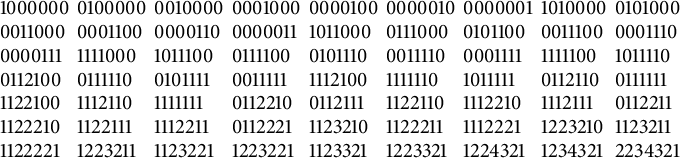 $$ \begin{align*} {\begin{array}{l@{\kern4pt}l@{\kern4pt}l@{\kern4pt}l@{\kern4pt}l@{\kern4pt}l@{\kern4pt}l@{\kern4pt}l@{\kern4pt}l}1 0 0 0 0 0 0& 0 1 0 0 0 0 0& 0 0 1 0 0 0 0& 0 0 0 1 0 0 0& 0 0 0 0 1 0 0& 0 0 0 0 0 1 0& 0 0 0 0 0 0 1& 1 0 1 0 0 0 0& 0 1 0 1 0 0 0\\[-.5pt] 0 0 1 1 0 0 0& 0 0 0 1 1 0 0& 0 0 0 0 1 1 0& 0 0 0 0 0 1 1& 1 0 1 1 0 0 0& 0 1 1 1 0 0 0& 0 1 0 1 1 0 0& 0 0 1 1 1 0 0& 0 0 0 1 1 1 0\\[-.5pt] 0 0 0 0 1 1 1& 1 1 1 1 0 0 0& 1 0 1 1 1 0 0& 0 1 1 1 1 0 0& 0 1 0 1 1 1 0& 0 0 1 1 1 1 0& 0 0 0 1 1 1 1& 1 1 1 1 1 0 0& 1 0 1 1 1 1 0\\[-.5pt] 0 1 1 2 1 0 0& 0 1 1 1 1 1 0& 0 1 0 1 1 1 1& 0 0 1 1 1 1 1& 1 1 1 2 1 0 0& 1 1 1 1 1 1 0& 1 0 1 1 1 1 1& 0 1 1 2 1 1 0& 0 1 1 1 1 1 1\\[-.5pt] 1 1 2 2 1 0 0& 1 1 1 2 1 1 0& 1 1 1 1 1 1 1& 0 1 1 2 2 1 0& 0 1 1 2 1 1 1& 1 1 2 2 1 1 0& 1 1 1 2 2 1 0& 1 1 1 2 1 1 1& 0 1 1 2 2 1 1\\[-.5pt] 1 1 2 2 2 1 0& 1 1 2 2 1 1 1& 1 1 1 2 2 1 1& 0 1 1 2 2 2 1& 1 1 2 3 2 1 0& 1 1 2 2 2 1 1& 1 1 1 2 2 2 1& 1 2 2 3 2 1 0& 1 1 2 3 2 1 1\\[-.5pt] 1 1 2 2 2 2 1& 1 2 2 3 2 1 1& 1 1 2 3 2 2 1& 1 2 2 3 2 2 1& 1 1 2 3 3 2 1& 1 2 2 3 3 2 1& 1 2 2 4 3 2 1& 1 2 3 4 3 2 1& 2 2 3 4 3 2 1 \end{array}}\end{align*} $$
The positive roots of the
 $\mathsf {E}_8$
root system are as follows.
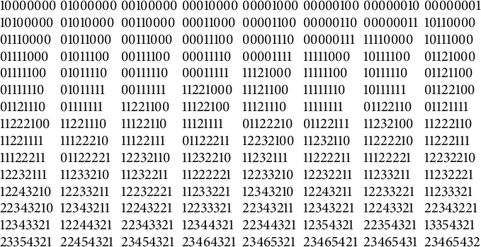 $$ \begin{align*} {\begin{array}{l@{\kern3pt}l@{\kern3pt}l@{\kern3pt}l@{\kern3pt}l@{\kern3pt}l@{\kern3pt}l@{\kern3pt}l}1 0 0 0 0 0 0 0& 0 1 0 0 0 0 0 0& 0 0 1 0 0 0 0 0& 0 0 0 1 0 0 0 0& 0 0 0 0 1 0 0 0& 0 0 0 0 0 1 0 0& 0 0 0 0 0 0 1 0& 0 0 0 0 0 0 0 1\\[-.5pt] 1 0 1 0 0 0 0 0& 0 1 0 1 0 0 0 0& 0 0 1 1 0 0 0 0& 0 0 0 1 1 0 0 0& 0 0 0 0 1 1 0 0& 0 0 0 0 0 1 1 0& 0 0 0 0 0 0 1 1& 1 0 1 1 0 0 0 0\\[-.5pt] 0 1 1 1 0 0 0 0& 0 1 0 1 1 0 0 0& 0 0 1 1 1 0 0 0& 0 0 0 1 1 1 0 0& 0 0 0 0 1 1 1 0& 0 0 0 0 0 1 1 1& 1 1 1 1 0 0 0 0& 1 0 1 1 1 0 0 0\\[-.5pt] 0 1 1 1 1 0 0 0& 0 1 0 1 1 1 0 0& 0 0 1 1 1 1 0 0& 0 0 0 1 1 1 1 0& 0 0 0 0 1 1 1 1& 1 1 1 1 1 0 0 0& 1 0 1 1 1 1 0 0& 0 1 1 2 1 0 0 0\\[-.5pt] 0 1 1 1 1 1 0 0& 0 1 0 1 1 1 1 0& 0 0 1 1 1 1 1 0& 0 0 0 1 1 1 1 1& 1 1 1 2 1 0 0 0& 1 1 1 1 1 1 0 0& 1 0 1 1 1 1 1 0& 0 1 1 2 1 1 0 0\\[-.5pt] 0 1 1 1 1 1 1 0& 0 1 0 1 1 1 1 1& 0 0 1 1 1 1 1 1& 1 1 2 2 1 0 0 0& 1 1 1 2 1 1 0 0& 1 1 1 1 1 1 1 0& 1 0 1 1 1 1 1 1& 0 1 1 2 2 1 0 0\\[-.5pt] 0 1 1 2 1 1 1 0& 0 1 1 1 1 1 1 1& 1 1 2 2 1 1 0 0& 1 1 1 2 2 1 0 0& 1 1 1 2 1 1 1 0& 1 1 1 1 1 1 1 1& 0 1 1 2 2 1 1 0& 0 1 1 2 1 1 1 1\\[-.5pt] 1 1 2 2 2 1 0 0& 1 1 2 2 1 1 1 0& 1 1 1 2 2 1 1 0& 1 1 1 2 1 1 1 1& 0 1 1 2 2 2 1 0& 0 1 1 2 2 1 1 1& 1 1 2 3 2 1 0 0& 1 1 2 2 2 1 1 0\\[-.5pt] 1 1 2 2 1 1 1 1& 1 1 1 2 2 2 1 0& 1 1 1 2 2 1 1 1& 0 1 1 2 2 2 1 1& 1 2 2 3 2 1 0 0& 1 1 2 3 2 1 1 0& 1 1 2 2 2 2 1 0& 1 1 2 2 2 1 1 1\\[-.5pt] 1 1 1 2 2 2 1 1& 0 1 1 2 2 2 2 1& 1 2 2 3 2 1 1 0& 1 1 2 3 2 2 1 0& 1 1 2 3 2 1 1 1& 1 1 2 2 2 2 1 1& 1 1 1 2 2 2 2 1& 1 2 2 3 2 2 1 0\\[-.5pt] 1 2 2 3 2 1 1 1& 1 1 2 3 3 2 1 0& 1 1 2 3 2 2 1 1& 1 1 2 2 2 2 2 1& 1 2 2 3 3 2 1 0& 1 2 2 3 2 2 1 1& 1 1 2 3 3 2 1 1& 1 1 2 3 2 2 2 1\\[-.5pt] 1 2 2 4 3 2 1 0& 1 2 2 3 3 2 1 1& 1 2 2 3 2 2 2 1& 1 1 2 3 3 2 2 1& 1 2 3 4 3 2 1 0& 1 2 2 4 3 2 1 1& 1 2 2 3 3 2 2 1& 1 1 2 3 3 3 2 1\\[-.5pt] 2 2 3 4 3 2 1 0& 1 2 3 4 3 2 1 1& 1 2 2 4 3 2 2 1& 1 2 2 3 3 3 2 1& 2 2 3 4 3 2 1 1& 1 2 3 4 3 2 2 1& 1 2 2 4 3 3 2 1& 2 2 3 4 3 2 2 1\\[-.5pt] 1 2 3 4 3 3 2 1& 1 2 2 4 4 3 2 1& 2 2 3 4 3 3 2 1& 1 2 3 4 4 3 2 1& 2 2 3 4 4 3 2 1& 1 2 3 5 4 3 2 1& 2 2 3 5 4 3 2 1& 1 3 3 5 4 3 2 1\\[-.5pt] 2 3 3 5 4 3 2 1& 2 2 4 5 4 3 2 1& 2 3 4 5 4 3 2 1& 2 3 4 6 4 3 2 1& 2 3 4 6 5 3 2 1& 2 3 4 6 5 4 2 1& 2 3 4 6 5 4 3 1& 2 3 4 6 5 4 3 2 \end{array}}\end{align*} $$
The positive roots of the
 $\mathsf {F}_4$
root system are as follows.
 $$ \begin{align*} &1 0 0 0&& 0 1 0 0&& 0 0 1 0&& 0 0 0 1&& 1 1 0 0&& 0 1 1 0&& 0 0 1 1&& 1 1 1 0&& 0 1 2 0&& 0 1 1 1&& 1 1 2 0&& 1 1 1 1\\& 0 1 2 1&& 1 2 2 0&& 1 1 2 1&& 0 1 2 2&& 1 2 2 1&& 1 1 2 2&& 1 2 3 1&& 1 2 2 2&& 1 2 3 2&& 1 2 4 2&& 1 3 4 2&& 2 3 4 2 \end{align*} $$
The positive roots of the
 $\mathsf {G}_2$
root system are as follows.
 $$ \begin{align*} &1 0&& 0 1&& 1 1&& 2 1&& 3 1&& 3 2 \end{align*} $$