INTRODUCTION
An increasing proportion of global biodiversity is located in fragmented tropical landscapes (Gibson et al. Reference GIBSON, LEE, KOH, BROOK, GARDNER, BARLOW, PERES, BRADSHAW, LAURANCE, LOVEJOY and SODHI2011); however, identifying the habitat spatial attributes with stronger impact on biodiversity has been challenging (Fahrig Reference FAHRIG2003). Forest patch size and isolation are known to affect the number of species (MacArthur & Wilson Reference MACARTHUR and WILSON1967) and metapopulation persistence (Hanski Reference HANSKI1999) in fragmented landscapes. Nevertheless, these effects depend on the landscape spatial context (e.g. percentage of remaining forest cover: Arroyo-Rodríguez et al. Reference ARROYO-RODRÍGUEZ, PINEDA, ESCOBAR and BENÍTEZ-MALVIDO2009, Bender & Fahrig Reference BENDER and FAHRIG2005, Pardini et al. Reference PARDINI, DE ARRUDA BUENO, GARDNER, PRADO and METZGER2010; matrix quality: Fahrig et al. Reference FAHRIG, BAUDRY, BROTONS, BUREL, CRIST, FULLER, SIRAMI, SIRIWARDENA and JEAN-LOUIS2011, Prugh et al. Reference PRUGH, HODGES, SINCLAIR and BRASHARES2008; landscape connectivity: Taylor et al. Reference TAYLOR, FAHRIG, HENEIN and MERRIAM1993). Thus, the distribution of species in an area is the result of processes operating at both patch and landscape spatial scales (Ricklefs Reference RICKLEFS1987), and hence, a multi-scale approach is required in fragmentation studies to accurately assess the effects of land-use change on biodiversity (Hill & Hamer Reference HILL and HAMER2004, Smith et al. Reference SMITH, FAHRIG and FRANCIS2011).
Tropical terrestrial mammals have an important role in preserving ecosystem integrity, especially in the Neotropics (Stoner et al. Reference STONER, RIBA-HERNÁNDEZ, VULINEC and LAMBERT2007, Terborgh et al. Reference TERBORGH, LÓPEZ, NUÑEZ, RAO, SHAHABUDDIN, ORIHUELA, RIVEROS, ASCANIO, ADLER, LAMBERT and BALBAS2001), and they represent an animal group particularly vulnerable to land-use change (Davidson et al. Reference DAVIDSON, HAMILTON, BOYER and CEBALLOS2009). Although many studies have evaluated changes in mammal assemblages in fragmented tropical landscapes, most assess the effects of patch metrics (Chiarello Reference CHIARELLO1999, Prugh et al. Reference PRUGH, HODGES, SINCLAIR and BRASHARES2008), without assessing (nor controlling) the effect of the landscape spatial pattern (but see McShea et al. Reference MCSHEA, STEWART, PETERSON, ERB, STUEBING and GIMAN2009, Thornton et al. Reference THORNTON, BRANCH and SUNQUIST2011a, Urquiza-Haas et al. Reference URQUIZA-HAAS, PERES and DOLMAN2009). The Lancandona rain forest in south-eastern Mexico harbours one of the highest numbers of mammal species in Mexico (Lira-Torres et al. Reference LIRA-TORRES, GALINDO-LEAL and BRIONES-SALAS2012, Medellín Reference MEDELLÍN1994). Although several studies have suggested that these animals may be threatened by land-use change in the area (Medellín Reference MEDELLÍN1994, Medellín & Equihua Reference MEDELLÍN and EQUIHUA1998, Tejeda-Cruz et al. Reference TEJEDA-CRUZ, NARANJO, CUARÓN, PERALES and CRUZ-BURGUETE2009), no study to date has evaluated the effect of the landscape spatial pattern on terrestrial mammals in the region.
Here, we assessed the relative effects of five landscape metrics (forest cover, number of forest patches, edge density, mean inter-patch isolation distance and matrix quality) and three patch metrics (patch size, shape and isolation) on medium- and large-sized terrestrial mammals in the fragmented Lacandona rain forest. We selected these metrics because it has been documented that they can negatively affect animal populations in fragmented landscapes (e.g. birds: Villard et al. Reference VILLARD, TRZCINSKI and MERRIAM1999; bats: Ethier & Fahrig Reference ETHIER and FAHRIG2011; primates: Arroyo-Rodríguez & Días Reference ARROYO-RODRÍGUEZ and DIAS2009; terrestrial mammals: Thornton et al. Reference THORNTON, BRANCH and SUNQUIST2011a). However, the responses of species to habitat configuration can be scale-dependent (Hill & Hamer Reference HILL and HAMER2004, Smith et al. Reference SMITH, FAHRIG and FRANCIS2011, Thornton et al. Reference THORNTON, BRANCH and SUNQUIST2011a), and hence, we measured the landscape metrics at two spatial scales, within 100-ha and 500-ha landscapes.
Our main objective was to identify the spatial attributes (and scales) with stronger influence on the number of species, as well as on the occurrence of each species. We tested three main hypotheses related to recent debates. First, we hypothesized that forest fragmentation (i.e. number of patches) will be substantially more important than forest loss, as fragmentation per se results in smaller forest patches and higher forest edge, and tropical species usually respond negatively to these habitat spatial patterns (Fahrig Reference FAHRIG2003, Thornton et al. Reference THORNTON, BRANCH and SUNQUIST2011a). Second, we tested if matrix quality had a significant and positive impact on the number and distribution of species; a topic that is receiving increasing attention (Fahrig et al. Reference FAHRIG, BAUDRY, BROTONS, BUREL, CRIST, FULLER, SIRAMI, SIRIWARDENA and JEAN-LOUIS2011, Melo et al. Reference MELO, ARROYO-RODRÍGUEZ, FAHRIG, MARTÍNEZ-RAMOS and TABARELLI2013, Perfecto & Vandermeer Reference PERFECTO and VANDERMEER2010, Santos-Filho et al. Reference SANTOS-FILHO, PERES, DA SILVA and SANAIOTTI2012). Finally, we tested if patch shape complexity and landscape edge density have a positive influence on diversity; a controversial topic because evidence indicates that the effects of these spatial attributes are as likely to be positive as negative (Ewers & Didham Reference EWERS and DIDHAM2006). We tested all these associations by controlling the influence of patch size and isolation, which are known to affect the distribution of species in fragmented landscapes (Hanski Reference HANSKI1999, MacArthur & Wilson Reference MACARTHUR and WILSON1967).
METHODS
Study area
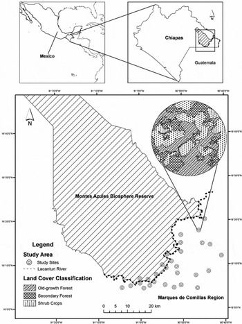
The Lacandona rain forest is located in the north-east of the state of Chiapas (16°05′58″N, 90°52′36″W) and is delimited by the Guatemalan border on the south and east, and by the Chiapas highlands on the north and west. The climate is hot and humid, with an annual precipitation average of 2850 mm, and average monthly temperatures of 24–26 °C. The Lacandona rain forest was originally covered by over 18000 km2 of rain forest, of which about 50% remains today (Bezaury-Creel & Gutiérrez-Carbonell Reference BEZAURY-CREEL and GUITIÉRREZ-CARBONELL2009). It is part of the Mesoamerican Biological Corridor, and represents a priority area for biodiversity conservation in Mexico and Mesoamerica (Myers et al. Reference MYERS, MITTERMEIER, MITTERMEIER, DA FONSECA and KENT2000). Within this region in 1978 the Montes Azules Biosphere Reserve (MABR) was created to protect the biodiversity. However, adjacent to the southern extreme of MABR, the Marqués de Comillas Region (MCR) was colonized about 40 y ago and since then MCR has suffered the rapid loss and fragmentation of the original rain forest because of uncontrolled land-use change (Mendoza & Dirzo Reference MENDOZA and DIRZO1999, Mora Reference MORA2008). Currently, the region is dominated by heterogeneous landscapes composed of different-sized rain-forest patches, embedded in a matrix of cattle pastures, agricultural lands (e.g. corn, oil palm, rubber) and human settlements. The study was conducted in the human-modified MCR (eastern side of the Lacantún river; 2039 km2) and the MABR (western side; 3312 km2) (Figure 1). The study was restricted to lowlands (100–200 m asl) formed in the Pleistocene by alluvial materials to control for confounding factors related to altitude and soil conditions. The weather conditions are also similar in the two areas.
Location of the study sites in the Lacandona rain forest in Chiapas south-eastern Mexico. We show the location of the 24 fragmented landscapes in the Marques de Comillas Region and the four control areas in the Montes Azules Biosphere Reserve. We described the landscape spatial pattern of all sites considering two different buffers (i.e. concentric circles) of 100 and 500 ha (see an example in the upper right side).

Study design and habitat spatial pattern
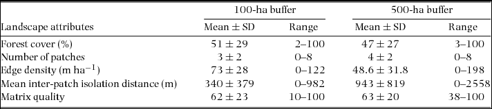
Following a growing number of fragmentation studies (Bender & Fahrig Reference BENDER and FAHRIG2005, Thornton et al. Reference THORNTON, BRANCH and SUNQUIST2011a, Umetsu & Pardini Reference UMETSU and PARDINI2007), we used a ‘landscape-patch’ approach (sensu McGarigal & Cushman Reference MCGARIGAL and CUSHMAN2002), in which response variables are taken from focal patches, but predictor variables (i.e. spatial attributes in this case) are measured from both patches and the surrounding landscape. In MCR we selected 24 fragmented focal patches of old-growth forest (3–80 ha) separated by at least 2 km from each other to increase independence among them (Figure 1). As controls, we also selected four buffer areas within the continuous old-growth forest in MABR (100 ha each) separated from each other by at least 4 km and at a minimum of 1 km from the Lacantún river (Table 1, Figure 1). With recent (March 2011) SPOT satellite images and the GIS GRASS program, we characterized the spatial configuration of the landscapes surrounding each site at two spatial scales: within a 100-ha buffer and within a 500-ha buffer from the centre of each sampling site (i.e. 100-ha and 500-ha landscapes, respectively; Figure 1). We used a supervised classification with GIS SPRING (Camara et al. Reference CAMARA, SOUZA, FREITAS and GARRIDO1996) considering six land-cover types: old-growth forests, secondary forests, tree crops (i.e. palm and rubber plantations), shrub crops (i.e. corn and bean plantations), cattle pastures and human settlements. Overall classification accuracy was 77%.
Landscape spatial attributes assessed in the Marqués de Comillas region, Lacandona rain forest, south-eastern Mexico for the 100-ha and 500-ha buffers. The landscapes sampled within the Montes Azules Biosphere Reserve were considered as control sites, i.e. with 100% of remaining forest cover, without forest patches nor forest edge, with complete connectivity (mean inter-patch isolation distance = 0 m), and maximum matrix quality (100).
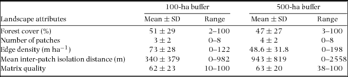
We used these two different buffer areas because the spatial extent at which landscape spatial pattern best predicts the response of species and populations (so-called ‘scale of effect’) varies across species (Jackson & Fahrig Reference JACKSON and FAHRIG2012). Following Jackson & Fahrig (2012), the radius of the landscape that best predicts population responses is 0.3–0.5 times the maximum dispersal distance (MDD) of the species. Thus, because MDD of most medium- and large-sized terrestrial mammals of the region ranges between 1000 and 4000 m (Bowman et al. Reference BOWMAN, JAEGER and FAHRIG2002, Sutherland et al. Reference SUTHERLAND, HARESTAD, PRICE and LERTZMAN2000, Thornton et al. Reference THORNTON, BRANCH and SUNQUIST2011b), the selected landscape sizes are adequate; i.e. 100-ha landscapes should allow evaluating the response of species with MDD between 1100 and 1900 m, meanwhile 500-ha landscapes should be appropriate for species with MDD between 2500 and 4200 m.
At the patch scale, we calculated the size, isolation and shape of all patches. Isolation distance was estimated as the distance to the nearest forest patch. Patch shape was calculated using the shape index: IF = P/√Aπ; where P and A are the patch perimeter and area, respectively (Forman & Godron Reference FORMAN and GODRON1986). The higher the IF values, the higher the shape complexity (perfect circle, IF = 1.0). Within each landscape (both at 100-ha and 500-ha scales) we estimated the percentage of remaining forest cover, number of forest patches, edge density (i.e. length of all old-growth forest borders within the landscape), mean inter-patch isolation distance (i.e. mean Euclidean nearest-neighbour distance of all patches to the focal patch in the landscape), and matrix quality. To estimate matrix quality we calculated an index that relates the percentage of each land-cover type within the landscape matrix to their relative quality. Because species presence declines along a land-use gradient (Gardner et al. Reference GARDNER, BARLOW, CHAZDON, EWERS, HARVEY, PERES and SODHI2009), the relative quality was ranked based on the vegetation structure of each land-cover type on a five-point scale: 1 (human settlements, lowest quality), 2 (cattle pastures), 3 (shrub crops), 4 (tree crops) and 5 (secondary forests, highest quality). This ranking was based on the generalized understanding of the positive effect of lower contrast between habitats surrounding a patch (e.g. because it can provide additional food resources or cover, as well as opportunities to disperse to other patches) (Gardner et al. Reference GARDNER, BARLOW, CHAZDON, EWERS, HARVEY, PERES and SODHI2009). Using this ranking, the quality index was calculated as: QI = [(1 × % human settlements) + (2 × % cattle pastures) + (3 × % shrub crops) + (4 × % tree crops) + (5 × % secondary forests)]/5.
Mammal surveys
From April to August 2011 we used camera traps, ground tracks and sightings to sample terrestrial mammal assemblages within each of the 28 sites. We used these three sampling methods because together they provide complementary information (Silveira et al. Reference SILVEIRA, JÁCOMO and DINIZ-FILHO2003) allowing us to have a rapid and more accurate estimation of the number of species within each site. We placed one motion-activated camera-trap (Cuddeback Capture®) within each patch in sites with signs of use by mammals. Each camera was left in that position for 30 d with a recovery time of 30 s per photograph. Every 30 d we downloaded the data and checked the cameras for battery, memory and performance. We then moved the camera to a different position within the same patch (0.06–1.10 km) (i.e. 30 d × 5 mo = 150 camera trap nights per patch, with five sample points in each patch). At the same time, ground tracks and sightings were performed once every 30 d by walking within each patch. AG and an experienced native guide surveyed the patch between 6h00 and 16h00, walking at a speed of about 1 km h−1. During these surveys all signs of medium- and large-sized terrestrial mammals including footprints, scats, or visual contact were recorded. We are particularly confident with the correct identification of signs because: (1) the field guide was a local hunter for most of his life and spends much of his time in the forest; (2) AG trained with two qualified researchers specializing in tropical mammals before field work; and (3) we used adequate field guides for corroborating species identifications (Aranda Reference ARANDA2000, Reid Reference REID2009). In order to cover as much area of a patch as possible, the length of the ground surveys was proportionate to the size of the patch (1 km for the smallest patch to ~7 km for the largest patch).
Data analysis
The study sites were considered independent samples because the landscapes (i.e. buffers) did not overlap in space (Eigenbrod et al. Reference EIGENBROD, HECNAR and FAHRIG2011). Furthermore, we applied a Mantel test to assess if the compositional similarity among sites (Jaccard index) was correlated with the inter-site variation in edge-to-edge isolation distances (ln-transformed), and we detected a very weak spatial autocorrelation (r = −0.1, P = 0.04).
To assess the accuracy of our mammal inventory, we first estimated the number of species expected for continuous and fragmented forests using the Chao-2 non-parametric estimator of species richness using the SPADE program (http://chao.stat.nthu.edu.tw/softwareCE.html). Subsequently, we calculated the percentage of species recorded within each forest condition (number of species observed/estimator × 100).
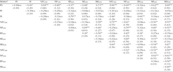
To identify the landscape and patch attributes with stronger influence on the number of species we used multiple regression analyses with generalized linear models (GLM) (Crawley Reference CRAWLEY2007). As suggested for count response variables, we fixed a Poisson error and a log link function, and corrected for data overdispersion (Crawley Reference CRAWLEY2007). To avoid collinearity between the predictor variables and multivariate models, we checked the relationship between all predictor variables with Pearson correlations, and each predictor's variance inflation factor (Neter et al. Reference NETER, KUTNER, NACHTSHEIM and WASSERMAN1996). Generally, a VIF > 4 indicates possible collinearity (Chatterjee et al. Reference CHATTERJEE, HADI and PRICE2000), and a VIF > 10 indicates severe collinearity (Neter et al. Reference NETER, KUTNER, NACHTSHEIM and WASSERMAN1996). These analyses indicated a possible collinearity between patch metrics and landscape metrics (Appendix 1), and hence, we performed three independent analyses: one for assessing the effect of patch metrics (patch size, shape and isolation), one for the 100-ha landscape metrics and one for the 500-ha landscape metrics. Because the number of patches was strongly correlated with the mean inter-patch isolation distance, both when considering the 100-ha (r = 0.89, P < 0.0001) and 500-ha (r = 0.93, P < 0.0001) landscapes (Appendix 1), we excluded the latter factor from multiple regressions. In each analysis we included distance walked in each site as a cofactor to control for differences among sites in sample size (Schoereder et al. Reference SCHOEREDER, GALBIATI, RIBAS, SOBRINHO, SPERBER, DESOUZA and LOPES-ANDRADE2004). We used the Akaike's Information Criterion (AIC) to select the most parsimonious model. We calculated the AIC corrected for small samples (AICc) for each model, and the model with the lowest AICc was considered the most plausible (Neter et al. Reference NETER, KUTNER, NACHTSHEIM and WASSERMAN1996).
To complement the results from GLMs, we also used regression trees calculated with the ‘tree’ library for R (v. 2.15.2) (R Core Team Development). Regression trees are useful when there are many explanatory variables and we need to identify which of them has the strongest impact on a continuous response variable (Crawley Reference CRAWLEY2007). They have been increasingly used in the ecological literature (Davidson et al. Reference DAVIDSON, HAMILTON, BOYER and CEBALLOS2009, Karp & Guevara Reference KARP and GUEVARA2011). In regression trees, the importance of each explanatory variable is assessed based on a recursive partitioning of the data into successively smaller groups with binary splits. The split (i.e. variable) explaining the greatest amount of the deviance in the response variable is selected and splitting continues until nodes are pure (i.e. they explain < 1% of the deviance) or the data have fewer than six observations (Crawley Reference CRAWLEY2007).
To identify the landscape and patch attributes with stronger influence on the distribution (presence/absence data) of each species we carried out Canonical Correspondence Analyses (CCA), one per spatial scale, with the MultiVariate Statistical Package for Windows (version 3.0). CCA is a simple method for arranging species along environmental variables, and is very useful for detecting species–environment relationships. It has been increasingly used in ecology because it seems to be immune to most of the problems of other ordination techniques, such as Correspondence Analysis and Detrended Correspondence Analysis (Palmer Reference PALMER1993). To prevent spurious effects caused by low population density and to minimize the risk of type II statistical errors, these analyses were performed only with species found in more than 20% of the sites (i.e. > six sites).
RESULTS
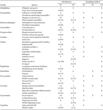
We recorded a total of 21 mammal species from 13 families (Table 2). Most species (18 species, 86%) were recorded in 2520 camera-trap nights, 16 species (76%) were recorded during 224 km of track surveys, and only six species (29%) were recorded through visual encounters (Table 2). Based on the Chao-2 non-parametric estimator, the average (± SE) accumulated number of species expected for continuous forest was 11.4 ± 1.1, and for forest fragments was 19.2 ± 0.7. Because we found a total of 11 species in continuous forest, and 19 species in forest fragments (Table 2), our mammal inventory can be considered accurate, with more than 95% of the species recorded within each forest condition.
Medium- and large-sized mammal species recorded with track surveys (TS), visual censuses (VC) and camera-traps (CT) in 24 forest patches and four sites within the continuous forest in the Lacandona rain forest, Mexico. Number and proportion (in parentheses) of sites occupied by each species in continuous (CF) and fragmented (FF) forests are indicated.

The species most widely distributed in both forest conditions were nine-banded armadillo (Dasypus novemcinctus), collared peccary (Pecari tajacu), paca (Cuniculus paca), white-tailed deer (Odocoileus virginianus) and red brocket deer (Mazama americana) (Table 2). In contrast, the jaguar (Panthera onca) and white-lipped peccary (Tayassu pecari) were recorded exclusively within the continuous forest, in two out of the four control sites.
Patch and landscape metrics affecting the number of species
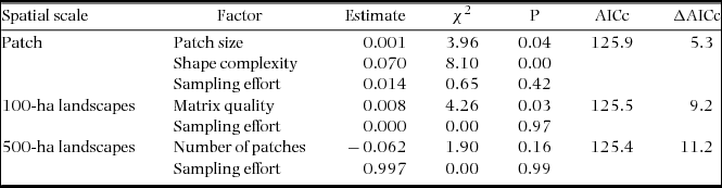
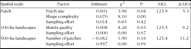
At the patch scale, the number of species increased principally with shape complexity (χ2 = 8.10, P = 0.004), but also with patch size (χ2 = 3.95, P = 0.046). When considering the 100-ha landscapes, the number of species increased in landscapes with higher matrix quality (χ2 = 4.2, P = 0.03). Finally, when considering the 500-ha landscapes, the minimal adequate model only included the number of patches (i.e. fragmentation), but its effect was not significant (χ2 = 1.89, P = 0.16) (df = 1 in all cases) (Table 3).
Results from generalized linear models to test the effect of landscape and patch metrics on assemblages of medium- and large-sized terrestrial mammals in the fragmented Lacandona rain forest, Mexico. We independently assessed the effects of three patch metrics (patch size, shape and isolation) and five landscape metrics (forest cover, number of forest patches, edge density, mean inter-patch isolation distance and matrix quality). In this last case we considered two different spatial scales: 100-ha landscapes and 500-ha landscapes. Only the minimal adequate model is included, i.e. the combination of predictor variables that based on the Akaike Information Criterion (corrected for small samples, AICc), best explained the number of species at each spatial scale. In all cases, we controlled for the effect of sampling effort. ΔAICc refers to the difference in AICc between full and minimal adequate models.
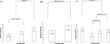
The regression trees supported the GLM results (Figure 2). At the patch scale, the regression tree explained 68.3% of the deviance in the number of species (Figure 2a). Shape complexity was the most important explanatory variable, and the threshold value separating low and high values of shape complexity was 8.1. The right-hand branch of the tree indicated that the average (± SE) number of species for high levels of shape complexity was 8 ± 0.9 species. The fact that this limb is unbranched means that no other variables explained a significant amount of the variation in the number of species for high values of shape complexity. When shape complexity was lower than 8.1, patch size affected positively the number of species; patches of less than 43.8 ha showed the lowest number of species (4.3 ± 0.6 species; Figure 2a).
Regression trees showing the spatial metrics that best explained the differences in the number of mammal species in the fragmented Lacandona rain forest, Mexico. Analyses were done at three spatial scales: patch scale (a); 100-ha landscape scale (b); and 500-ha landscape scale (c). The length of each branch is proportionate to the node's percentage of total deviance reduction. On each node (split), the name of the explanatory variable and its threshold value are indicated. The bars at the tips of the terminal nodes (leaves) show the mean values (± SE) of the number of species in that subset of data (the number of data points is indicated within each bar). Spatial metrics: Shape = shape complexity; Psize = patch size; MQ = matrix quality; F = fragmentation (number of forest patches); and E = edge density. The 100 and 500 numbers refers the 100-ha and 500-ha landscapes.

At the 100-ha landscape scale, the regression tree explained 82.1% of the deviance. This model showed that the number of species was mainly related to matrix quality; the number of species increased in landscapes with a matrix quality higher than 61.7 (6.7 ± 0.6 species) than in landscapes with a matrix quality below this threshold (4.7 ± 0.5 species; Figure 2b). Finally, at the 500-ha landscape scale, the model explained 62.2% of the deviance (Figure 2c). At this scale, the number of species was negatively impacted by fragmentation level, as landscapes with less than 3.5 patches (left-hand branch) maintained the highest number of species (6.6 ± 0.7 species). Interestingly, above this fragmentation threshold, matrix quality and edge density showed positive effects on the number of species. In fact, the lowest number of species was recorded in landscapes with higher fragmentation level, but with lower matrix quality and edge density (4.0 ± 0. 8 species; Figure 2c).
Patch and landscape metrics affecting the occurrence of each species
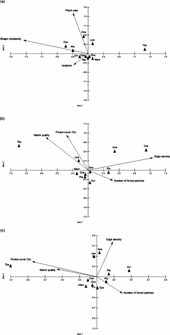
The first two eigenvalues of CCA at the patch, 100-ha and 500-ha scales explained 95.9%, 90.7% and 72.5% of the variation in mammal composition, respectively (Figure 3). At the patch scale, shape complexity was the spatial factor with the strongest impact on species composition (Figure 3a), positively affecting the occurrence of the northern naked-tailed armadillo (Cabassous centralis) and the raccoon (Procyon lotor), but negatively affecting the occurrence of T. bairdii. The presence of N. narica and the ocelot (Leopardus pardalis) was positively associated with patch size (Figure 3a). At the 100-ha landscape scale, matrix quality, forest cover and edge density were the spatial factors with greatest influence on the distribution of mammals (Figure 3b). The presence of T. bairdii was positively associated with matrix quality and forest cover, whereas C. centralis and N. narica occupied landscapes with higher edge density. Finally, at the 500-ha landscape scale, the spatial metric with strongest effect on mammal assemblages was the percentage of forest cover, with a positive effect on the occurrence of T. bairdii (Figure 3c). In contrast, O. virginianus, P. tajacu and P. lotor occupied more frequently landscapes with lower forest cover, whereas the occurrence of N. narica and L. pardalis was positively related to edge density.
CCA ordination diagrams displaying the mammal species recorded in the Lacandona rain forest, Mexico and its relationship with different spatial metrics (arrows) estimated at the patch (a), 100-ha landscape (b) and 500-ha landscape (c) scales. Each arrow points in the direction of maximum change of that spatial metric across the diagram, and its length is proportionate to the rate of change in this direction (i.e. spatial metrics with longer arrows are more closely related to the pattern of species distribution shown in the ordination diagram). Mammal species: Cce = Cabassous centralis; Cpa = Cuniculus paca; Dno = Dasypus novemcinctus; Lpa = Leopardus pardalis; Mam = Mazama americana; Nna = Nasua narica; Ovi = Odocoileus virginianus; Pta = Pecari tajacu; Plo = Procyon lotor; Tba = Tapirus bairdii.

DISCUSSION
The importance of patch shape complexity
The number of mammal species increased principally with shape complexity at the patch scale. This factor can have both negative and positive effects on diversity (reviewed by Ewers & Didham Reference EWERS and DIDHAM2006). The negative effects are related to the increment of the perimeter/area relationship, and the potential negative impact that this process can have on numerous biotic and abiotic processes near forest edges (so-called edge effects; Laurance et al. Reference LAURANCE, LOVEJOY, VASCONCELOS, BRUNA, DIDHAM, STOUFFER, GASCON, BIERREGAARD, LAURANCE and SAMPAIO2002, Murcia Reference MURCIA1995). Thornton et al. (Reference THORNTON, BRANCH and SUNQUIST2011a) actually argue that landscapes with greater edge density can be of lower quality for tropical terrestrial mammals because, among other threats, animals in such a situation may be more exposed to human persecution and unfavourable habitat in the matrix. However, both habitat heterogeneity and the primary productivity associated with secondary forests near forest edges can be higher in more complex patches, increasing resource availability for many species (Martínez-Morales Reference MARTÍNEZ-MORALES2005). Also, the likelihood that species will enter in the matrix and use complementary or supplementary resources from it may be higher in more complex-shaped patches (Dunning et al. Reference DUNNING, DANIELSON and PULLIAM1992). Additionally, patches with more irregular shapes have a higher probability of being randomly occupied by a given individual, increasing the colonization rates within these patches (Ewers & Didham Reference EWERS and DIDHAM2006). Finally, shape complexity in the Lacandona region is usually associated with the presence of rivers and streams, and hence, the presence/abundance of water bodies within patches with more complex shapes could attract a larger number of medium- and large-sized mammals. Therefore, although more studies are necessary to assess the generality of our results, the positive effects of patch shape complexity seems to be substantially more important than the negative effects, at least in study regions such as ours, with a relatively high remaining forest cover (c. 50%) distributed in small and large forest patches (> 1000 ha) embedded in a heterogeneous matrix.
The number of mammal species also increased with patch size, but mainly when patches showed a more compact (circular) shape (Figure 2). This means that the threats associated with more compact patches may be counterbalanced if patch size increases. For example, habitat diversity and resource availability are known to be greater in larger patches (Arroyo-Rodríguez & Mandujano Reference ARROYO-RODRÍGUEZ and MANDUJANO2006, Báldi Reference BÁLDI2008, Zanette et al. Reference ZANETTE, DOYLE and TREMONT2000). The probability of patch colonization also increases with patch size (Hanski Reference HANSKI1999, MacArthur & Wilson Reference MACARTHUR and WILSON1967). Furthermore, larger patches may suffer less forest degradation resulting from low-intensity logging (Bawa & Seidler Reference BAWA and SEIDLER2008, Chapman & Peres Reference CHAPMAN and PERES2001), and maintain larger populations (Estrada & Coates-Estrada Reference ESTRADA and COATES-ESTRADA1996, Verbeylen et al. Reference VERBEYLEN, BRUYN and MATTHYSEN2003) with lower probability of extinction (Fischer & Lindenmayer Reference FISCHER and LINDENMAYER2007, Hanski Reference HANSKI1999). Overall, this body of evidence can help to explain why smaller and more compact patches showed the lower number of mammal species.
The importance of matrix quality
Particularly interesting was the fact that, considering the 100-ha landscapes, matrix quality was the main factor influencing the number of species. Although an increasing number of studies have highlighted the importance of matrix quality for the maintenance of diversity in fragmented landscapes (Fahrig et al. Reference FAHRIG, BAUDRY, BROTONS, BUREL, CRIST, FULLER, SIRAMI, SIRIWARDENA and JEAN-LOUIS2011, Melo et al. Reference MELO, ARROYO-RODRÍGUEZ, FAHRIG, MARTÍNEZ-RAMOS and TABARELLI2013, Perfecto & Vandermeer Reference PERFECTO and VANDERMEER2010), very few studies have demonstrated that matrix quality is positively related to the number of terrestrial mammals in tropical fragmented forests (Santos-Filho et al. Reference SANTOS-FILHO, PERES, DA SILVA and SANAIOTTI2012). This factor can facilitate inter-patch animal movement, and affect important ecological dynamics for diversity maintenance in fragmented landscapes (Dunning et al. Reference DUNNING, DANIELSON and PULLIAM1992, Fahrig et al. Reference FAHRIG, BAUDRY, BROTONS, BUREL, CRIST, FULLER, SIRAMI, SIRIWARDENA and JEAN-LOUIS2011). For example, some animals can persist in relatively unsuitable patches when they are able to use complementary or supplementary resources located outside of their home patch (i.e. in the matrix) (Antongiovanni & Metzger Reference ANTONGIOVANNI and METZGER2005, Asensio et al. Reference ASENSIO, ARROYO-RODRÍGUEZ, DUNN and CRISTÓBAL-AZKARATE2009, Dunning et al. Reference DUNNING, DANIELSON and PULLIAM1992). In this sense, the higher number of species in patches surrounded by matrices with a greater proportion of tree crops and secondary forests (i.e. higher quality) could be associated with the fact that many mammal species in the region are habitat generalists (e.g. D. novemcinctus, O. virginianus, P. tajacu) and often use food resources from these kinds of vegetation cover (Parry et al. Reference PARRY, BARLOW and PERES2007, Tejeda-Cruz et al. Reference TEJEDA-CRUZ, NARANJO, CUARÓN, PERALES and CRUZ-BURGUETE2009).
The relative impact of forest loss and forest fragmentation
Our findings support the hypothesis that in the tropics forest fragmentation is substantially more important than forest loss (Fahrig Reference FAHRIG2003). The generalized linear models suggest that at the 500-ha landscape scale, only forest fragmentation tended to be negatively associated with the number of species (Table 3). This tendency was supported by regression trees (Figure 2), which indicated that fragmentation was the main factor influencing negatively the number of species at this scale. Thornton et al. (Reference THORNTON, BRANCH and SUNQUIST2011a) also find that fragmentation per se has a negative impact on many terrestrial mammal species in a fragmented tropical landscape in Guatemala, most probably because of the loss of landscape connectivity in more fragmented landscapes (Appendix 1). Inter-patch animal movements and metapopulation dynamics are interrupted with decreasing connectivity (Hanski Reference HANSKI1999). Other key landscape-scale processes that are critical for species survival in fragmented landscapes and that can be altered with decreasing connectivity are source-sink dynamics and landscape complementation/supplementation (Dunning et al. Reference DUNNING, DANIELSON and PULLIAM1992).
In this sense, it was very interesting that under high levels of forest fragmentation, the number of species was positively related to matrix quality and edge density (Figure 2). As argued above, these two landscape characteristics can increase landscape connectivity, increasing patch colonization rates and resource availability (Ewers & Didham Reference EWERS and DIDHAM2006). Thus, matrix quality and edge density can also be important factors for the maintenance of mammal assemblages at larger spatial scales, particularly when landscapes are strongly fragmented.
Species-specific responses to forest cover change
Overall, our results support the idea that there is a gradient of tolerance to forest cover change, from species greatly sensitive to species tolerant of (or even benefited by) forest-cover change (Hill & Hamer Reference HILL and HAMER2004, Thornton et al. Reference THORNTON, BRANCH and SUNQUIST2011a, Urquiza-Haas et al. Reference URQUIZA-HAAS, PERES and DOLMAN2009). The jaguar, white-lipped peccary and Baird's tapir were the most sensitive to habitat loss, as the former two were only recorded within continuous forest sites, and the latter only occurred in two out of 24 (8%) patches. In fact, the probability of occurrence of Baird's tapir increased in landscapes with higher forest cover and higher matrix quality in 100-ha and 500-ha landscapes. These three large-bodied species have large home-range requirements and live in relatively small densities, both of which are biological attributes usually associated with a higher vulnerability to land-use change (Daily et al. Reference DAILY, CEBALLOS, PACHECO, SUZAN and SÁNCHEZ-AZOFEIFA2003, Naranjo Reference NARANJO2009, but see Thornton et al. Reference THORNTON, BRANCH and SUNQUIST2011a).
The ocelot and white-nosed coati occurred in both continuous and fragmented forests (Table 2); however, the probability of patch occupancy by these species was positively associated with patch size (Figure 3). The presence of ocelots also increased in 100-ha landscapes with greater forest cover. Thornton et al. (Reference THORNTON, BRANCH and SUNQUIST2011a) also find that the occurrence of these two species is associated with larger patches. Although the ocelot can occur in fragmented forests, it prefers closed-canopy forests (Jackson et al. Reference JACKSON, LAACK and ZIMMERMAN2005), which are typical of larger forest patches (Arroyo-Rodríguez & Mandujano Reference ARROYO-RODRÍGUEZ and MANDUJANO2006). The coati is a semi-arboreal species and also inhabits essentially forested habitats, feeding mainly on fruits (Gompper Reference GOMPPER1995), which are expected to be less available in smaller forest patches (Arroyo-Rodríguez & Mandujano Reference ARROYO-RODRÍGUEZ and MANDUJANO2006). Therefore, although these species were relatively more tolerant to land cover loss, they were dependent on the presence of large forest patches.
Finally, several species showed a high tolerance to forest cover change. For example, the raccoon and northern naked-tailed armadillo were positively related to shape complexity and edge density. In fact, the occurrence of the raccoon was positively related to forest fragmentation while the armadillo was only present in forest patches. The raccoon is a well-known generalist species that commonly uses resources from habitat edges and the landscape matrix. Habitat use by the northern naked-tailed armadillo is poorly understood, but this species is known to inhabit secondary forests and agricultural fields (Cuarón Reference CUARÓN, Ceballos and Oliva2005). In fact, the few records of this species of armadillo in the study region are from open areas and roads near agricultural fields (González-Zamora et al. Reference GONZÁLEZ-ZAMORA, ARROYO-RODRÍGUEZ, GONZÁLEZ, LOMBERA, PEÑA, PEÑA, HERNÁNDEZ-ORDOÑEZ, MUENCH and STONER2011), suggesting that this species makes use of habitat edges for feeding or travel. The white-tailed deer and collared peccary also use resources from open areas (e.g. crops) (Keuroghlian & Eaton Reference KEUROGHLIAN and EATON2008, Tejeda-Cruz et al. Reference TEJEDA-CRUZ, NARANJO, CUARÓN, PERALES and CRUZ-BURGUETE2009), and we found that they were positively associated with forest fragmentation and negatively related to forest cover in 100-ha and 500-ha landscapes. Therefore, these species could be benefited by a moderate degree of forest-cover loss in the landscape (Tejeda-Cruz et al. Reference TEJEDA-CRUZ, NARANJO, CUARÓN, PERALES and CRUZ-BURGUETE2009, Thornton et al. Reference THORNTON, BRANCH and SUNQUIST2011a, Urquiza-Haas et al. Reference URQUIZA-HAAS, PERES and DOLMAN2009).
Recommendations for conservation
Our findings demonstrated that more complex-shaped and larger patches, and particularly those surrounded by a greater proportion of secondary forests and tree crops (i.e. with more quality matrix), maintained a higher number of species of medium- and large-sized terrestrial mammals. Therefore, if current land use aimed at replacing forest with pastures continues (Mendoza & Dirzo Reference MENDOZA and DIRZO1999, Mora Reference MORA2008) it is very likely that the number of mammal species will decline, particularly the habitat specialists (Hill & Hamer Reference HILL and HAMER2004, Thornton et al. Reference THORNTON, BRANCH and SUNQUIST2011a, Urquiza-Haas et al. Reference URQUIZA-HAAS, PERES and DOLMAN2009). This process could alter key ecological relationships (e.g. seed dispersal, seed predation and the preservation of food webs), threatening the maintenance of ecosystem integrity (Stoner et al. Reference STONER, RIBA-HERNÁNDEZ, VULINEC and LAMBERT2007, Terborgh et al. Reference TERBORGH, LÓPEZ, NUÑEZ, RAO, SHAHABUDDIN, ORIHUELA, RIVEROS, ASCANIO, ADLER, LAMBERT and BALBAS2001). Therefore, it is necessary to preserve larger and complex-shaped patches (e.g. those connected with riparian corridors) and increase tree cover within the matrix (Umetsu & Pardini Reference UMETSU and PARDINI2007). This management strategy can increase landscape connectivity, thus favouring inter-patch movements, as well as key ecological dynamics for diversity maintenance in fragmented landscapes (Dunning et al. Reference DUNNING, DANIELSON and PULLIAM1992, Fahrig et al. Reference FAHRIG, BAUDRY, BROTONS, BUREL, CRIST, FULLER, SIRAMI, SIRIWARDENA and JEAN-LOUIS2011). To enhance the conservation value of our assessment, future studies in the area should monitor population trends over time to have a better understanding of the impact of land-use changes on species persistence.
ACKNOWLEDGEMENTS
This research was supported by a grant from the Dirección General de Asuntos del Personal Académico, DGAPA, Universidad Nacional Autónoma de México, UNAM (project IA-203111). A. Garmendia obtained a scholarship from the Consejo Nacional de Ciencia y Tecnología (CONACyT), as part of the Programa de Posgrado en Ciencias Biológicas of UNAM. The Centro de Investigaciones en Ecosistemas, UNAM provided logistical support. We thank to A. Navarrete for providing the SPOT images and C. Dobler for digitizing the maps. Three anonymous reviewers provided very thoughtful advice. This study would not have been possible without the collaboration of the local people in Loma Bonita, Chajul, Reforma Agraria, Zamora Pico de Oro, Ixcán, 13 de septiembre, Playón la Gloria, Galacia, San Isidro, El Porvenir, El Pirú, Tierra y Libertad, Flor de Marqués de Comillas, Adolfo López Mateos, Santa Rita and La Nueva Unión. We especially thank A. Jamangape for his invaluable field assistance. G. Sánchez, H. Ferreira, A. Palencia, A. López and C. Correa provided technical support.
Pearson correlation coefficients and variance inflation factor (in parentheses) among landscape metrics (i.e. percentage of forest cover, %FC, number of forest patches, NP, edge density, ED, mean inter-patch isolation distance, MI, and matrix quality, MQ) and patch metrics (patch size, PS, patch isolation, PI, and shape index, SI) used to characterize the spatial configuration of the study sites. Subscript 100 and 500 indicate the 100-ha and 500-ha landscapes. n.s., not significant (P > 0.05), * P < 0.05, ** P < 0.01, *** P < 0.001.