


This paper introduces three new metrics, namely, the solvency assets multiple (SAM), the funded assets multiple (FAM), and the risk-free funded ratio (RFFR). These metrics can augment the classic funded ratio, allowing for a more comprehensive assessment of the health of a liability-based plan (LBP). They can be based on static investment strategies or even optimized dynamic investment strategies. We present examples that show how these metrics explicitly account for a variety of sources of stochasticity that cannot be taken into account in the funded ratio, such as randomness in equity returns, interest rates, and inflation. The new metrics enable determining the sensitivity of a plan’s health to these and other factors.
We define LBPs to encompass any plan whose primary investment goal is to fulfill a set of liabilities to be paid over the course of years, like a pension. LBPs include liability-driven investing (LDI), liability aware investing (LAI), and asset-liability management (ALM). The distinction between these three categories is not a sharp one but is generally connected to how stochastic the liabilities are assumed to be and how stochastic the assets are allowed to be. LDI is generally viewed as the most conservative of the three. Its liabilities are often assumed to be fixed, and the assets comprise large proportions of bonds for cash-flow matching. ALM is generally the least conservative. ALM often allows for a wide range of asset classes to match liabilities, which are assumed to have varying levels of stochasticity. In typical ALM, the use of equities in the asset portfolio is allowed to be widespread. LAI lies in between LDI and ALM.
While these distinctions between LDI, LAI, and ALM are not completely concrete nor agreed upon, what matters more in the context of this paper is that, regardless of these distinctions, all LBPs employ asset management approaches that are liability-focused, with the primary concern of maintaining a high probability of meeting the liabilities.Footnote 1 This institutional investing priority has interesting parallels to goals-based wealth management (GBWM) for single or multiple goals, in which an optimal investment plan, and, in addition for multiple goals, an optimal goals fulfillment strategy, is determined for individual investors (as in Das et al. (Reference Das, Ostrov, Radhakrishnan and Srivastav2020) and Das et al. (Reference Das, Ostrov, Radhakrishnan and Srivastav2022)). For example, a common previous application of GBWM has been to enable individuals to optimize their defined contribution (DC) plans, but, as we will show in this article, it can also be applied to help pension firms support defined benefit (DB) plans. This comes from the simple recognition that paying all the LBP’s liabilities can be thought of as a goal to be attained from a GBWM context (which the SAM metric will address), or, alternatively, paying each year’s liability can be thought of as separate goals to be attained (which the FAM metric will address).
While LBPs take varied investment approaches, there is a standard metric commonly used for the health of these plans. This metric is the funded ratio of the plan, which is defined by
 \begin{equation*}
\mbox{Funded ratio} = \frac{\mbox{Current assets}}{\mbox{Current liabilities}},
\end{equation*}
or some variation of this equation. The ‘Current assets’ in the numerator is straightforward to calculate. It is the current market worth of the plan’s assets. But the ‘Current liabilities’ in the denominator, also referred to as the projected benefit obligation (PBO), is not as clearly determined, because liabilities are to be paid in the future, and therefore, after the amounts of the future liabilities are estimated, they must be present-valued using a discount rate,  $D$. The discount rate is a point of much contention. Currently, a fixed value for
 $D$ (usually in the 6–8% range) is chosen to present-value all liabilities, irrespective of their maturities.
Determining if a pension plan is sufficiently funded is a crucial issue that has important ramifications for the plan’s participants. If it is determined that a plan has a shortfall that the plan sponsor cannot address, it may mean forced reductions in entitlements for pensioners. Persistent underfunding over a number of years is a significant warning sign, as is significant volatility in a plan’s health. In the case of public plans, persistent underfunding can place additional burdens on future taxpayers or lead to benefit reductions for new or even current employees. This is why there is extensive regulatory disclosure required of pension plans, with the desire for these disclosures to give a true sense of the plan’s ability to pay future liabilities.
The trigger for further scrutiny of a plan under the United States Pension Protection Act is having a pension plan with a funded ratio below 80 percent, which is a standard many plans fail to meet (see Aubry and Munnel (Reference Aubry and Munnel2025)). For example, as of the end of the 2023 fiscal year, state and local pension plans had 5.07 trillion dollars in assets but 1.61 trillion dollars in unfunded liabilities, with a median funded ratio of 75 percent.Footnote 2 Further, pension plan funded ratios are fragile to shocks. For example, the average funded ratio for state and local pensions was 92.4 percent in 2007, which then fell to 62.4 percent in 2009 due to the Great Recession, and has not come close to fully recovering since then.Footnote 3 Of course, funded ratio changes like these will affect both public pensions and private DB plans. Our analyses in this paper apply to both public and private plans. Private DB plans, which are shrinking, have Pension Benefit Guarantee Commission backing, while public plans pose a greater risk to tax payers when they become unhealthy.
However, using the funded ratio as the sole metric of a plan’s financial health potentially fails to take into account a number of important financial issues that we will detail in Section 2. As the American Academy of Actuaries (AAA) Senior Pension Fellow Don Fuerst stated, ‘Any realistic assessment of a pension plan should include several measures, not just one.’Footnote 4 The AAA’s 2017 issue brief ‘Assessing Pension Plan Health: More Than One Right Number Tells The Whole Story’Footnote 5 is even more clear, stating that:
A single number often cannot comprehensively address an issue as complex as the obligation or funded status of a pension plan. The availability of multiple measurements can lead to a more robust understanding of the situation and more well-reasoned conclusions. Understanding that there is more than one right number is an essential step toward engaging in critical issues of retirement security.
This AAA brief then recommends two additional types of measurements, without providing specifics. One type would ‘represent an estimate of how much money the plan would need to have in order for a projection to show that the assets are expected to be sufficient to cover projected benefit payments’, noting that ‘such an estimate is inherently uncertain’. The other type would ‘rel[y] only on financial information available in today’s financial markets’ and would be connected ‘to show[ing] how much it would cost a plan sponsor to transfer the responsibility of supporting a plan to an insurance company or other financial institution’.
In this paper, we develop three new metrics. The first two of our metrics, which are distinctive in that they are based on the probability of meeting the plan’s liabilities, fit perfectly with the first type of measurement recommended above by the AAA, while our third metric fits perfectly with the second type of AAA-recommended measurement. We next give basic descriptions of these three metrics.
The first metric is the SAM. Here we look for  $\alpha$, the minimum constant multiple of the current assets and, if desired and the plan is open, future projected contributions needed to attain a specified probability of meeting all the plan’s future liabilities. We then define SAM to be
 $\frac{1}{\alpha}$, the reciprocal of
 $\alpha$. We define SAM by the reciprocal of
 $\alpha$, as opposed to
 $\alpha$ itself, so that it parallels the funded ratio in that a high number is good, and a low number is bad. Also, in both SAM and the funded ratio, a value of one means that we are projected to barely meet our goal with the current resources.
The second metric is the FAM. It is defined the same way as SAM, except that instead of looking to attain a specified probability of meeting all the plan’s future liabilities, we now look to attain specified probabilities for meeting each year’s future liabilities. This has the advantage of being able to specify higher required probabilities for meeting liabilities in early years and lower probabilities in later years, where long-term investments like stock may be more appropriate.
The third metric is the RFFR. We define RFFR the same way the funded ratio is defined, except that instead of a constant discount rate being used to present-value all the liabilities, we use the yield curve for United States Treasury STRIPS to present-value each year’s liability separately and we also use this yield curve to present-value any future contributions, which we add to the current assets. Because we use STRIPS, RFFR is the ratio of the current plan’s worth to the amount needed by the plan to lock in payments of all the future liabilities, assuming those are fixed values. This makes RFFR a highly relevant metric for institutions currently considering buying or selling an LBP. In practice, because future liabilities are often made uncertain by inflation, an LBP’s RFFR generally needs to attain a specific value greater than 1, such as 1.3, before the company owning the LBP can immunize themselves by transferring their plan to another institution willing to take it over. We will look to compute the cumulative probability over time that RFFR reaches this immunization value, guaranteeing the plan’s remaining liabilities will be met.
Because, as the 2017 AAA brief points out, there is inherent uncertainty involved with SAM and FAM, we require models for any stochastic features like inflation or how investments evolve that are used to determine SAM or FAM. These must be determined by the companies managing the LBPs (or regulatory agencies). RFFR, on the other hand, only depends on financial information available in the market, as the AAA recommended, namely the yield curve for STRIPS.
The organization of this paper is as follow. In Section 1, we discuss previous research on metrics for the health of LBPs and methods to optimize these metrics. In Section 2, we will discuss the pros and cons of the funded ratio and our new metrics, showing how they work well in concert with each other. In Section 3, we give an overview of how SAM and FAM are calculated. In Section 4, we show how Monte Carlo simulation can be used to compute our three metrics in the context of a plan where we know the investment strategy and have a variety of sources of uncertainty. We will also discuss the insights that these three metrics provide. In Section 5, we go a step farther, showing how dynamic programming can be used to determine the optimal investment strategy that maximizes SAM or that maximizes FAM. We make some brief concluding comments in Section 6.
1. Previous research on measuring and optimizing plans with liability-based goals
Pension plans are required to report their funded ratio, in an effort to make public whether the plan is underfunded or overfunded. The present value of liabilities depends on the discount rate applied for discounting. The PPA (Pension Protection Act of 2006)Footnote 6 and FASB (United States Financial Accounting Standards Board) Statement 158Footnote 7 require plan sponsors to fund any shortfalls over certain time horizons and report their liabilities and funding status directly on their balance sheets. The term structures most commonly used for discounting liabilities are the IRS (Internal Revenue Service) Discount Curve, which is used for the PPA, and the Citigroup Pension Discount Curve, which is used for FASB 158. Both term structures are based on the yields of high-quality (investment grade) United States dollar corporate bonds; thus, they reflect both interest rate risk and credit spread risk.
The most common metric in addition to the funded ratio that is used in practice is surplus volatility, meaning the volatility of the assets minus the discounted liabilities. Some papers, such as Sharpe and Tint (Reference Sharpe and Tint1990); Ezra (Reference Ezra1991), and Delong et al. (Reference Delong, Gerrard and Haberman2008), have considered methods to maximize the funded ratio minus a constant multiple of surplus volatility. Butt (Reference Butt2012) presents a multidimensional simulation study to analyze the volatility of DB pension funds’ funding ratios. Ang et al. (Reference Ang, Chen and Sundaresan2013) also incorporates downside risk, but through adding a penalty that is proportional to the value of an option that is in the money when the funded ratio drops below one. Cannon and Tonks (Reference Cannon and Tonks2013) undertakes a cross-country comparison of the risks and funded ratios of pension plans, finding that the risk of wage growth and its effect on returns is so substantial that only strategies that are heavily equity loaded have a reasonable chance of remaining funded. Insurance approaches, which are addressed in Broeders and Chen (Reference Broeders and Chen2013), are likely to reduce the shortfall probability and the expected loss given a shortfall, but they also lower the probability of high positive returns. Boyce and Ippolito (Reference Boyce and Ippolito2002) argues that such insurance schemes are too costly.
Previous research on pension fund management strategy suggest that the optimal investment strategy is sensitive to its constraints, for example, Van Binsbergen and Brandt (Reference Van Binsbergen, Brandt and Veronesi2016) and Martellini and Milhau (Reference Martellini and Milhau2012). Stockton et al. (Reference Stockton, Donaldson and Shtekhman2008) approaches LDI by looking to meet a plan’s liabilities while constraining the volatility of the funded ratio over time. This can be done by exact cash-flow matching (best for frozen funds) or duration matching, or some combination of the two. Exact matching is difficult because employee turnover, inflation, mortality, and salaries can alter the liabilities, so that it is a moving target. While the risk of employee turnover cannot be hedged, at least duration matching can be used to alleviate much of the interest rate risk that is incurred when creating targeted cash-flows to match uncertain liabilities. Upbin et al. (Reference Upbin, Stefanelli and Gendron2012) presents a series of benchmark LDI indexes with target durations between six and sixteen years, against which pension fund performance may be benchmarked.
The optimization literature regarding LDI almost exclusively looks to optimize the expected value of a traditional utility function. While static optimization was originally used, dynamic optimization is now far more common (Huang, Reference Huang2010). Cox et al. (Reference Cox, Lin, Tian and Yu2013) minimizes the expected value of the funding variation, that is,  $E\left[\sum\limits_{t=1}^{\infty}\left(\frac{U(t)}{(1+\rho)^t} \right)^2 \right]$, where
 $\rho$ is a discount rate and
 $U(t)$ stands for the unfunded liabilitiesFootnote 8 in year
 $t$. This is done by determining the optimal asset weights and the optimal normal contribution value. Similar objectives are used by Delong et al. (Reference Delong, Gerrard and Haberman2008). Josa-Fombellida and Rincón-Zapatero (Reference Josa-Fombellida and Rincón-Zapatero2008) considers the optimal management of an aggregated dynamic pension fund, with multiple classes of workers with stochastic salaries (Chang and Cheng, Reference Chang and Cheng2002). Their objective is to minimize the cost of contributions and maximize the utility of the final surplus, measured as the relative fund level with respect to the mean salary, which is a proxy for the replacement rate.Footnote 9
Josa-Fombellida et al. (Reference Josa-Fombellida, López-Casado and Rincón-Zapatero2018) use different objective functions depending on whether the plan is overfunded or underfunded – when the plan is initially underfunded, the objective is to minimize  $E[(X(T))^2]$, the expected square of the negative surplus,
 $X$, at the fund’s horizon time,
 $T$. But when the plan is initially overfunded, the objective is to maximize
 $E\left[\frac{(X(T))^{1-\xi}}{1-\xi}\right]$, the expected power law utility of the positive surplus,
 $X$, at the fund’s horizon, where
 $\xi \gt 0$ is the risk aversion coefficient. In Mao and Wen (Reference Mao and Wen2021), the expected shortfall per unit cumulative wealth is minimized using CVaR. The flip side of this objective would be to maximize the replacement rate, which is a proxy for maximizing the surplus. Devolder et al. (Reference Devolder, Princep and Fabian2003) use a variety of utility functions to study the optimal investment strategy of a plan using annuities to target its liabilities in an ALM setting. Battocchio and Menoncin (Reference Battocchio and Menoncin2004), followed by Ma (Reference Ma2011), examines optimal investment strategies for maximizing the exponential utility of a DB plan’s final wealth when interest rates and inflation are stochastic.
Our approach to measuring and optimizing the health of an LBP fund in this paper differs in that we do not look to optimize traditional utility functions, because those functions do not connect to the core goal of LBP funds, which is to optimize the probability of meeting its liabilities. Our RFFR metric, for example, directly connects to the ability to completely immunize a plan (Biffis and Blake, Reference Biffis and Blake2013), meaning there is a 100 percent chance of meeting its liabilities, or at least to better inform potential buyers of pension plans looking at undergoing a pension risk transfer for de-risking.Footnote 10 Our SAM and FAM metrics are directly connected to the probabilities of meeting either all or each of the fund’s liabilities, respectively.
While SAM and FAM appear to be ‘break-point’ metrics in that they do not consider the extent of shortfall conditional on the inability to meet liabilities, they are still continuous in the asset levels of funds, hence they do not have discontinuities in measuring the health of a fund. They offer one approach in which probabilities of a shortfall may be converted into a metric. An alternative acceptable approach would be to translate expected shortfall into a metric. Both metrics, while correlated with the funded ratio, address different aspects of LBP health (discussed next in Section 2). The event of failure to meet liabilities (akin to bankruptcy) is far more critical than the extent of shortfall when failure occurs. This is because of regulatory and legal triggers, financial impact, and social consequences of a default. It is legally critical for pensions to meet obligations, because even a partial failure could trigger lawsuits, court-ordered payments, or even constitutional crises (in the case of public funds). A plan that cannot meet its scheduled liabilities, even with a modest shortfall, can trigger downgrades, raising borrowing costs.
Concerns about using the funded ratio as the sole metric of an LBP’s health have arisen from a variety of sources. For example, Sgouros (Reference Sgouros2017) lists a number of these concerns in the context of funding public pensions, and he presents recommendations for pension accounting standards reform in Sgouros (Reference Sgouros2019). Concerns about solely using the funded ratio have also been discussed by the AAA, leading to their publishing two issue briefsFootnote 11 regarding what they refer to as the ‘80% funding myth’, by which they mean that ‘[f]requent unchallenged references to [an] 80% fund[ed ratio] as a healthy level threaten to create a mythic standard’. Our additional metrics can help address these concerns.
2. Balancing the pros and cons of the funded ratio with our new metrics
Let  $A$ represent the current worth of assets in an LBP and
 $L(t)$ represent the liability owed by the plan
 $t$ years from now (for
 $t=1,2,...$), where
 $L(t)$ is in present-valued dollars, so it needs to be adjusted by inflation over the
 $t$ years. Assuming a constant projected rate of inflation,
 ${\hat\pi}$, and a constant discount rate,
 $D$, the formula for the funded ratio is simply
 \begin{equation}
\mbox{Funded ratio} = \frac{\mbox{Current assets}}{\mbox{Current liabilities}}
= \frac{A}{\sum\limits_{t=1}^{\infty}L(t)e^{({\hat\pi}-D)t}
}.
\end{equation}
One of the key advantages of the funded ratio is the simplicity of this formula. It is easy to understand and only requires two constants,  ${\hat\pi}$ and
 $D$, to be calculated. The ease of understanding the formula makes it particularly useful, both to regulators and the parties bound by the LBP. The meaning of a change to
 ${\hat\pi}$ or
 $D$ is clear. But the simplicity of the formula also means we miss a number of important financial features that we want our new metrics, even if they are more complicated, to address.
In particular, determining the appropriate discount rate  $D$ for the funded ratio is a particularly difficult task because it must reflect so many financial factors, which cannot be supported by a single number like
 $D$ that is deterministic and constant over time. As Sgouros (Reference Sgouros2019) states, the funded ratio should ‘not combine low-accuracy numbers (liability) with high-accuracy numbers (assets) and expect to get anything but a very rough estimate, unsuitable as a basis for making important decisions’.
Because the constant  $D$ does not vary with time, it cannot apply a different rate to short-term liabilities versus long-term liabilities. This ignores the shape of the yield curve, and it ignores the differences in short-term versus long-term asset holdings (that is, the glide path of the portfolio). Further, the funded ratio does not reveal anything about the timing of the liabilities, except through the discount rate. A funded ratio of 80 percent is not remotely as serious a concern if the liabilities are due 30 years from now, as opposed to if the liabilities are due 1 year from now.
The discount rate is, by definition, a projected expected return on the plan’s overall assets over the horizons of the liabilities, just as  ${\hat \pi}$ is a projected expected rate of inflation over the liabilities. The discount rate should reflect the risk, return, and duration characteristics of the cash flow (in this case, the liabilities) being discounted. Even if the projected expected return is completely accurate for some reason, the discount factor cannot take into account the volatility of the returns. That is, the funded ratio does not take into account stochastic effects.
This lack of accounting for stochastic effects means the funded ratio cannot help determine better ways to invest LBP funds so they can better meet their liabilities. In fact, the advice the funded ratio suggests is completely inappropriate for LBP funds: Since riskier investment portfolios have a higher expected return, they correspond to a higher value of  $D$, which means a higher funded ratio. That is, the more risky the investment portfolio, the healthier the plan will seem to be according to the funded ratio, even though LBP plans should be particularly sensitive to the dangers that such additional volatility creates.Footnote 12
Further, because the funded ratio does not address stochastic effects, it cannot take notions of probability into account. That is, the value of the funded ratio does not translate to a specific understanding of the probability that the LBP will not be able to pay its liabilities. Because the probability of paying liabilities is such a key part of understanding the health of an LBP plan, our SAM and FAM metrics work extensively with these probabilities that the funded ratio cannot address.
For the RFFR, we simply replace the constant discount rate,  $D$, in the funded ratio formula (1) with
 $y(t)$, the yield to time
 $t$ for United States Treasury STRIPS:
 \begin{equation}
\mbox{RFFR}
= \frac{A}{\sum\limits_{t=1}^{\infty} L(t)e^{({\hat \pi}-y(t))t}
}.
\end{equation}
There is no uncertainty about  $y(t)$ since it is available by simply looking at the market’s current yield curve. The only uncertainty that remains in the RFFR formula is
 ${\hat \pi}$. Aside from this inflation uncertainty, the key weakness of the RFFR is that it only accommodates STRIPS. It says nothing about stochastic investments.
Both the SAM and the FAM require algorithms, as opposed to formulas, to be computed, but they can say a great deal about stochastic investments and other stochastic factors. These algorithms can be as simple as using Monte Carlo methods if we have a fixed investment portfolio strategy, or they can involve more complex dynamic programming methods when we consider optimally switching among a variety of investment portfolio possibilities. In Section 3, we describe both of these methods and their uses.
No matter the method, SAM and FAM have many advantages that augment our understanding of the health of an LBP plan because they address stochastic behavior and probabilities. More specifically, they can work with stochastic models for investment returns and for inflation, including models that change over time if desired. They also determine probabilities of meeting the liabilities, taking into account when each liability is due. Further, they can produce the optimal investment portfolio choices for maximizing these probabilities, knowing that the investment portfolio choice can be changed each year in the future, depending on future market conditions.
That is, SAM and FAM are excellent at addressing the primary deficiencies of the funded ratio. However, SAM and FAM require specifying the models for investment returns and inflation. Choosing accurate models poses one difficulty; choosing accurate parameters within the models poses another.Footnote 13 The simplicity of the funded ratio means there are only two constants to agree upon. The complexity of return models and their parameters in SAM and FAM means there is far more to agree upon to determine them. Further, the fact that SAM and FAM require an algorithm, as opposed to a simple formula like the funded ratio or RFFR, means that the effect of changing the return models or their parameters, while computable, is less intuitive.
Augmenting the funded ratio: The funded ratio can be altered to consider the effect of projected new assets (e.g., infusions from future contributions),  $A_p(t)$, and projected new liabilities (e.g., those created by future employees),
 $L_p(t)$. We will refer to this altered version as the augmented funded ratio:
 \begin{align}\mbox{Augmented funded ratio} & = \frac{\mbox{Current assets + projected assets}}{\mbox{Current liabilities + projected liabilities}} \nonumber \\
& = \frac{A + \sum\limits_{t=1}^{\infty}A_p(t)e^{({\hat \pi}-D)t}}{\sum\limits_{t=1}^{\infty}(L(t)+L_p(t))e^{({\hat \pi}-D)t}
}.\end{align}
Of course, a similar alteration can be made to define the augmented RFFR. The augmented funded ratio can be useful, for example, in understanding how new projected contributions can improve the funded ratio. We will use it for examples later in the paper where we have projected assets, but not projected liabilities, meaning the augmented funded ratio is higher than the funded ratio. That is, the augmented funded ratio will suggest the LBP is healthier than the funded ratio in this case.
One disadvantage of the augmented funded ratio is that it does not make a distinction between projected assets arriving before or after liabilities occur, which, of course, can significantly affect if a liability can be paid. In our examples, we have made certain this potential timing issue with the augmented funded ratio does not occur. Both SAM and FAM, on the other hand, automatically address these timing concerns by keeping track of when infusions occur and when liabilities are paid. That is, neither can allow liabilities to be paid with infusions projected to occur after the liability is due. We note that in all our metrics, these projected assets and liabilities do not need to be taken into account if it is felt they do not reflect the actual health of the LBP. In particular, uncertainty in these projections can be an excellent reason not to include them, in which case we use the standard versions of the funded ratio and RFFR, not the augmented versions.
The new metrics proposed here are related to Actuarial Standards of Practice (ASOP No. 4), which already suggests that multiple measurements may be made and should be reported carefully (see Sections 2.13 and 4.1(p)), keeping in mind different purposes of measurement (Section 3.3).Footnote 14 We note that SAM and FAM directly satisfy ASOP requirements to consider volatility, uncertainty, and timing of obligations (Sections 3.5.3 and 3.15 of ASOP No. 4).
RFFR embodies the market-consistent present value framework, which ASOP requires actuaries to disclose when used. ASOP distinguishes between asset-based present values (Section 3.7.1, discounting at expected return) and ‘market-consistent present values’ (Section 3.7.3, using observable yields not related to the asset strategy of the plan). By using STRIPS, the RFFR is a specific objective form of market-consistent liability valuation that the ASOP explicitly contemplated as one acceptable measure. ASOP requires disclosure of whether the actuary used an asset-based or non-asset-based present value method (Section 4.1(i)); RFFR is strongly in line with this requirement. All three metrics enhance compliance with ASOP Section 4.1(q), which requires actuaries to warn that ‘future actuarial measurements may differ significantly’, since SAM and FAM quantifications of probabilities automatically illustrate those differences. Thus, the new metrics are consistent with ASOP No. 4; they operationalize its guidance and would enhance compliance, especially with risk assessment and disclosure obligations.
We give an overview of how SAM and FAM are determined in the next section.
3. An overview of calculating SAM and FAM
In this section, we give an overview of the approaches we will use to compute SAM and FAM in Sections 4 and 5. In Section 4, we will consider a case where the investment portfolio strategy is fixed. In Section 5, we will consider a case where we consider optimally switching among a variety of investment portfolios over time. Because the investment strategy is fixed in Section 4 but can move and needs to be dynamically optimized in Section 5, our approaches for computing SAM and FAM in the two sections will be considerably different.
In Section 4, we will use a simple Monte Carlo approach to compute SAM and FAM. That is, we determine a stochastic model for the movement of stocks, bonds, and inflation, and then we use these stochastic models to run a large number (10,000 in our case) of simulations, which determines the (approximate) probability of our desired outcomes. Because Monte Carlo methods use simulation that evolves forward in time, our stochastic models do not have to be Markovian. That is, the evolution of the market and inflation can depend on previous history, not just the current state of a few relevant variables. We will employ a geometric Brownian motion model for stock evolution and a Vasicek model for bond evolution and inflation evolution.
For SAM, we start with a given acceptable probability,  $P_{\rm br}$, of going bankrupt (hence the subscript ‘br’) before meeting all the liabilities. We start with the current assets,
 $A$, and, if desired, the projected assets,
 $A_p(t)$, and determine the fraction of the simulations that lead to bankruptcy. If the fraction is higher than
 $P_{\rm br}$, we rerun the Monte Carlo simulation with
 $\alpha=2$, meaning we start with
 $2 \times A$ current assets and
 $2\times A_p(t)$ projected assets; if the fraction is lower than
 $P_{\rm br}$, we rerun the Monte Carlo simulation with
 $\alpha=\frac{1}{2}$. Either way, between the initial run (with
 $\alpha =1$) and the new run (with
 $\alpha = 2$ or
 $\frac{1}{2}$), we now have two
 $\alpha$ values and their corresponding probabilities of going bankrupt. From there, we just apply the secant method for root finding to determine the
 $\alpha$ value that corresponds to the acceptable probability of going bankrupt,
 $P_{\rm br}$. The value of SAM is the reciprocal of this value of
 $\alpha$. For reasons explained in Subsection 4.5, we will use a slightly different version of FAM in Section 4 that uses the same algorithm just described for SAM; however, the secant method is used to find the smallest
 $\alpha$ where the cumulative (‘cum’) probabilities of going bankrupt each year stay below given acceptable probabilities,
 $P_{\rm br, cum}(t)$. Normally FAM requires the probabilities of not meeting each year’s liability to remain below given acceptable (‘acc’) probabilities,
 $P_{\rm acc}(t)$, which are not cumulative.
In Section 5, we consider an example where we allow switching each year among different investment portfolios. Because of this, Monte Carlo simulation becomes inappropriate since there are so many potential future investment portfolio paths to compare, even if the number of investment choices available each year is small. Indeed, the computational time Monte Carlo would require for our example would exceed by many orders of magnitude the age of the universe, which is 13.8 billion years. Dynamic programming, on the other hand, is capable of determining the optimal investment portfolio strategy within a couple of minutes.
Dynamic programming accomplishes this by using the Bellman (Reference Bellman1952) equation to generate solutions backward in time over a dense mesh of wealth values at each time. We explain this further, first for SAM. Our method for determining SAM follows Das et al. (Reference Das, Ostrov, Radhakrishnan and Srivastav2020), which we summarize as follows:
We start at time  $t=T-1$, the year before the final liability is due at time
 $T$. For each wealth value in the mesh at time
 $T-1$, we determine and select the investment portfolio over the final year (i.e.,
 $t\in(T-1,T))$ that maximizes the probability of attaining the money needed to pay the final liability at time
 $T$. These probabilities follow from the dynamics; that is, from the model for the stochastic evolution of each investment portfolio. We will use the geometric Brownian motion model for our dynamics. The expected return and volatility parameters in the geometric Brownian motion model will differ with each available investment portfolio that can be selected. Although it is not required for our algorithm, we will restrict ourselves to investment portfolios whose expected returns and volatilities correspond to points along the efficient frontier. At the end of this process, each wealth value in the mesh at time
 $T-1$ will have the optimal investment portfolio assigned to it, as well as the optimal probability of paying the final liability.
We then move backward a year to time  $T-2$. For each point in the wealth mesh at time
 $T-2$, we want to determine which investment portfolio is best to select for
 $t\in(T-2,T-1)$ (that is, the next year) to attain the goal of SAM, which is to pay all our remaining liabilities. This is done by comparing the effect of each possible investment portfolio selection for the next year on the probability of paying the final two years of liabilities (that is, paying
 $(L(T-1) + L_p(T-1))e^{{\hat \pi}(T-1)}$ and
 $(L(T) + L_p(T))e^{{\hat \pi}T}$). To determine this probability for each investment portfolio selection, (1) we first determine the distribution of the wealth values that will be attained at the beginning of time
 $T-1$ (which depends on the investment portfolio selection), then (2) we add
 $\alpha \times A_p(T-1)e^{{\hat \pi}(T-1)}$ and subtract
 $(L(T-1) + L_p(T-1))e^{{\hat \pi}(T-1)}$, noting that bankruptcy occurs if subtracting
 $(L(T-1) + L_p(T-1))e^{{\hat \pi}(T-1)}$ leads to a negative wealth, and (3) finally, if our remaining wealth is positive at time
 $T-1$, we use interpolation between the two closest wealth mesh points at time
 $T-1$ to this remaining wealth to obtain the optimal probability of paying off the final liability,
 $(L(T) + L_p(T))e^{{\hat \pi}T}$. At the end of this, each wealth value in the mesh at time
 $T-2$ will have the optimal investment portfolio for the next year assigned to it, as well as the optimal probability of paying both of the liabilities in the final two years.
We repeat this process, going backward one year at a time, until we reach the current time,  $t=0$. With each iteration backward in time, we are determining the optimal investment portfolio at each wealth value in the mesh one year earlier than before, as well as the optimum probability of paying all the remaining liabilities given that we have the mesh point’s wealth at this time. Once we reach
 $t=0$ in our computation, we simply look at the optimal probability of paying all liabilities at the point in the wealth mesh corresponding to
 $\alpha \times A$. To optimally run the portfolio, each year we simply look at the remaining wealth in the portfolio after paying the liability and select the optimal investment portfolio corresponding to the closest wealth mesh point at that time. As before, SAM is the reciprocal of the value of
 $\alpha$, where the wealth
 $\alpha \times A$ at
 $t=0$ is a wealth mesh point whose optimum probability of paying all the remaining liabilities is
 $1-P_{\rm br}$.
Our method for determining FAM follows Das et al. (Reference Das, Ostrov, Radhakrishnan and Srivastav2022). In this method, utility values are assigned to each liability, where the connection between the probability of attaining a liability and the utility value assigned to the liability will follow Das et al. (Reference Das, Ostrov, Radhakrishnan and Srivastav2023). We next summarize this approach:
We first assign utility values to each year’s combined liability, meaning that we include the projected liabilities for the year if they exist. The utility value corresponds to how important spending money to pay the (combined) liability is for that year. We temporarily defer how these utility values are determined, noting for now that the higher the utility assigned to a liability, the higher the probability of paying the liability, but the lower the probability of paying the other liabilities in general. For FAM, in contrast to SAM, our goal is to maximize the expected value of the sum of the utilities of paid liabilities between the current year,  $t=0$, and the final year,
 $t=T$.
The backward iteration method for FAM based on the Bellman equation follows the method for SAM outlined above, with the following alterations: Once we have the optimal investment portfolio for each wealth value in the mesh of wealth values at time  $T-1$ (which is determined as we did for SAM), we also determine at each wealth value in this mesh if it is optimal to pay the liability,
 $(L(T-1) + L_p(T-1))e^{{\hat \pi}(T-1)}$, or not. This is done by first adding the infusion at time
 $T-1$, which is
 $\alpha \times A_p(T-1)e^{{\hat \pi}(T-1)}$, to the wealth value and then seeing what is bigger: (1) the expected utility if we don’t pay the liability at time
 $T-1$, which is computed by taking the product of the utility assigned to the final liability at time
 $T$ and the optimal probability of paying that liability given the wealth of the new mesh point at time
 $T-1$ (meaning the closest mesh point after adding
 $\alpha \times A_p(T-1)e^{{\hat \pi}(T-1)}$) or (2) the total expected utility if we do pay the liability at time
 $T-1$, which is computed by taking the utility assigned to the liability at time
 $T-1$ and adding to it the product of the utility assigned to the final liability at time
 $T$ and the optimal probability of paying that liability given the wealth of the new mesh point at time
 $T-1$ (meaning the closest mesh point after adding
 $\alpha \times A_p(T-1)e^{{\hat \pi}(T-1)}$ and then subtracting the liability
 $(L(T-1) + L_p(T-1))e^{{\hat \pi}(T-1)}$). Whichever of these two expected utility totals is higher dictates the optimal decision regarding whether or not to pay the liability for time
 $T-1$ at the wealth mesh point in question (prior to the infusion) at time
 $T-1$.
In other words, for each wealth mesh point (prior to adding  $\alpha \times A_p(T-1)e^{{\hat \pi}(T-1)}$) at time
 $T-1$, we now know what the optimal strategy is: that is, whether or not it is better to pay the time
 $T-1$ liability, and then what the best investment portfolio to choose for the next year is. We also know for each wealth mesh point at time
 $T-1$ the optimal expected utility from paid liabilities at times
 $T-1$ and
 $T$.
For a point in the wealth mesh at time  $T-2$, we follow a nearly identical pattern: we first determine at each wealth point in the mesh what investment portfolio leads to the highest expected utility. The expected utility corresponding to an investment portfolio is determined by taking the sum over each mesh point at time
 $T-1$ of the product of the optimal expected utility determined for the time
 $T-1$ wealth mesh point and the probability (given by the investment portfolio) of reaching that time
 $T-1$ wealth mesh point from the starting wealth mesh point of interest at time
 $T-2$. Once the optimal investment portfolio is known, we, as before, compare the expected utility if we do or do not pay the time
 $T-2$ liability to determine if is optimal to pay the time
 $T-2$ liability or not.
We then know for each wealth mesh point at time  $T-2$ what the optimal strategy is (i.e., whether or not to pay the liability and what investment portfolio to select) and what the optimal expected utility is from paid liabilities at time
 $T-2$ or later. As in SAM, we then iterate this method backward one year at a time until we reach the present time,
 $t=0$. After this, we start at the wealth mesh corresponding to
 $\alpha \times A$ at
 $t=0$ and work forward in time using the optimal choices for paying liabilities and the optimal investment portfolio selection choices. This yields the probabilities that each liability will be paid. FAM, as discussed above, is the reciprocal of the minimum value of
 $\alpha$ where the wealth
 $\alpha \times A$ at
 $t=0$ corresponds to the probabilities of not meeting each year’s liability remaining below the given acceptable probabilities,
 $P_{\rm acc}(t)$.
We now return to the question ‘How do we determine the utilities that we assign to each liability?’ For any specific, fixed value of  $\alpha$ that we are considering, in our first run, we assign the same utility to every goal. This generates probabilities of paying each year’s liability. The paper Das et al. (Reference Das, Ostrov, Radhakrishnan and Srivastav2023) shows how to update the utilities by comparing them to
 $1-P_{\rm acc}(t)$, the minimum acceptable probabilities of paying each liability. In particular, it gives a sense for how much to increase the utilities for each liability where the probability is below
 $1-P_{\rm acc}(t)$ and decrease the utilities for each liability where the probability is above
 $1-P_{\rm acc}(t)$. This leads to a new run, and then this process is repeated for more new runs until all the probabilities are above
 $1-P_{\rm acc}(t)$ or all the probabilities are below
 $1-P_{\rm acc}(t)$. The amount they all are above or below gives a sense for how much to change
 $\alpha$, and then we repeat this entire process. As before, this corresponds to a root finding process where we use the secant method to obtain the desired
 $\alpha$ to compute FAM.
Throughout the dynamic programming process, we are determining the optimal probability of paying all remaining liabilities (for SAM) or the optimal expected utility from paid current and future liabilities (for FAM) at each state, meaning each wealth and time point. The fact that we only have two states (wealth and time) is key to our ability to use dynamic programming. While in theory it is possible to use more states, the computational time grows exponentially as the number of states increases, meaning three states takes a very long time and four states or more is essentially impossible. This exponential blow up in computational time when working backward in time with dynamic programming (the ‘curse of dimensionality’) corresponds to the exponential blow up in computational time working forward in time with Monte Carlo methods when we allow switching between investment portfolios each year.
To describe the evolution of inflation over time, the Vasicek model requires two state variables (the current inflation rate at time  $t$ and the accumulated inflation up to time
 $t$). The Vasicek model also requires two state variables to describe the evolution of bond prices over time. We cannot address the resulting six state variable model (i.e., wealth and time plus the four states from the two Vasicek models) with dynamic programming. Fortunately, we know from reinforcement learning (RL) that historical inflation in America is well approximated in analyses like ours by a constant value (see Das et al. (Reference Das, Khadilkar, Mittal, Ostrov, Srivastav and Wang2026)). Further, we can approximate the evolution of investment portfolios that contain combinations of stocks and bonds by using geometric Brownian motion models, especially when the bond fraction is small, as in most LBPs. This removes the need for the additional state variables the Vasicek model requires, so we can stay with just two state variables for wealth and time, as we do in Section 5 when we use dynamic programming. We note that if we do wish to use the Vasicek model for inflation and for bonds – meaning six state variables – and we also want to determine and use the optimal investment portfolio and pay liabilities optimally, then RL becomes an appropriate technique for approximating solutions, as shown in Das et al. (Reference Das, Khadilkar, Mittal, Ostrov, Srivastav and Wang2026).
4. Computing and analyzing the metrics for a fixed investment strategy example
In this section, we consider funds with a fixed portfolio strategy. For example, an LDI fund might have a fixed strategy of 90 percent bonds and 10 percent stock. Target date funds are another example of a fixed strategy, because even though the fractions of their underlying components change over time, they do so in a specified (fixed) way.
Because the portfolio strategy is fixed, Monte Carlo simulation is an effective tool to gauge the effect of a variety of sources of randomness that can affect the performance of the fund and its ability to pay liabilities. In our examples in this section, we will consider three sources of randomness: movement in the stock market, changes to the inflation rate, and changes to the yield curve for interest rates. We note that we could also easily include the effects of varying mortality rates or uncertainty in contribution rates, bond defaults, etc. Our model will only consider investing in a total stock market index fund and AA rated corporate bonds. Again, we note that we could easily expand our model to include the effect of additional assets like commodities, derivative securities, international stocks, high-yield bonds, TIPS (Treasury Inflation-Protected Securities), treasury bonds, etc. To calculate RFFR, our model will also need to use STRIPS.
For our fixed portfolio strategy, we look to use Monte Carlo simulation to calculate SAM or FAM or to determine the likelihood of being able to immunize a plan if it attains a sufficiently high RFFR and can therefore be sold. To do this, we must describe the nature of the plan and our assumptions for modeling both our sources of uncertainty and for the fixed portfolio strategy. We do this first for SAM and FAM. We will later discuss the additional modeling necessary for the STRIPS needed to determine RFFR.
4.1. Model dynamics
We consider three sources of randomness in the framework:
• Stock: For simplicity, we assume the stock component’s price evolves by geometric Brownian motion, which means that
 $S(t)$, the stock component’s price at time
$t$, where
$t$ is measured in years, is governed by the stochastic differential equation
where
\begin{equation*}dS=\mu S dt+ \sigma S dW,\end{equation*}
$W$ is a Wiener process and
$\mu$ and
$\sigma$ are the expected return and volatility of the stock. The solution to this stochastic differential equation is
where
\begin{equation*}S(t+1) = S(t)e^{\mu-\frac{\sigma^2}{2} + \sigma Z_1},\end{equation*}
$Z_1$ is a standard normal random variable. We have chosen
$\mu=7$ percent and
$\sigma=20$ percent as an example of a forecast for these parameters if the stock represents a total stock index.
• Inflation: We assume that inflation evolves by the Vasicek (Reference Vasicek1977) model, which means that
$\pi(t)$, the rate of inflation at time
$t$, is governed by the stochastic differential equation
(4)where this equation’s Wiener process,\begin{equation}
d\pi = \kappa_{\pi}(\theta_{\pi} -\pi)dt+\sigma_{\pi} dW,
\end{equation}
$W$, is independent of the Wiener process in the geometric Brownian motion model. The Vasicek model is an Ornstein–Uhlenbeck process (Uhlenbeck and Ornstein, Reference Uhlenbeck and Ornstein1930) for mean reversion, where
$\theta_{\pi}$ is the mean value of
$\pi$,
$\kappa_{\pi}$ is the strength of the reversion to this mean value, and
$\sigma_{\pi}$ is a constant representing the strength of the randomness. The solution to equation (4) is
(5)where\begin{equation}
\pi(t+1) = \pi(t)e^{-\kappa_{\pi}} + \theta_{\pi}(1-e^{-\kappa_{\pi}}) + \sigma_{\pi}\sqrt{\frac{1-e^{-2\kappa_{\pi}}}{2\kappa_{\pi}}} Z_2,
\end{equation}
$Z_2$ is a standard normal random variable that is independent of
$Z_1$. Zhang and Ewald (Reference Zhang and Ewald2010) derive an optimal investment strategy for a pension fund facing inflation. As an example of a forecast for the parameters in our model, we have chosen
$\kappa_{\pi} = 0.6, \theta_{\pi} = 0.025,$ and
$\sigma_{\pi} = 0.03$, loosely based on United States inflation rate data between 1955 and 2023. We have also chosen an initial inflation rate of 2 percent.• The yield curve for zero-coupon AA corporate bonds: We assume that
$r_{_{\textrm{AA}}}(t)$, the instantaneous interest rate of AA corporate bonds at time
$t$, is also governed by the Vasicek model, but with the restriction that it cannot become negative; therefore, from equation (5), we have that
(6)where\begin{equation}
r_{_{\textrm{AA}}}(t+1) = \max\left\{0, r_{_{\textrm{AA}}}(t)e^{-\kappa_{\rm{AA}}}
+ \theta_{_{\textrm{AA}}}(1-e^{-\kappa_{\rm{AA}}})
+ \sigma_{_{\textrm{AA}}}\sqrt{\frac{1-e^{-2\kappa_{\rm{AA}}}}{2\kappa_{_{\textrm{AA}}}}} Z_3 \right\},
\end{equation}
$Z_3$ is a standard normal random variable that is independent of
$Z_1$ and
$Z_2$. Further, as shown in Mamon (Reference Mamon2004) for example, this implies that
$ZCB_{_{\textrm{AA}}}(t,T)$, the cost of a zero-coupon AA corporate bond at time
$t$ that will be worth $1 at time
$T$, is given by
(7)where\begin{equation}
ZCB_{_{\textrm{AA}}}(t,T) = e^{B(t,T) - r_{\rm{AA}}(t)A(t,T)},
\end{equation}and
\begin{equation*}A(t,T) = \frac{1}{\kappa_{_{\textrm{AA}}}}\big(1-e^{-\kappa_{\rm{AA}}(T-t)}\big)
\end{equation*}
\begin{equation*}
B(t,T) = \left(\theta_{_{\textrm{AA}}} - \frac{\sigma_{_{\textrm{AA}}}^2}{2\kappa_{_{\textrm{AA}}}^2} \right)\big(A(t,T)-T+t\big) - \frac{\sigma_{_{\textrm{AA}}}^2}{4\kappa_{_{\textrm{AA}}}} A^2(t,T).
\end{equation*}As an example of a forecast for these Vasicek model parameters for AA corporate bonds, we have chosen
$\kappa_{_{\textrm{AA}}} = 0.5, \theta_{_{\textrm{AA}}} = 0.035,$ and
$\sigma_{_{\textrm{AA}}} = 0.02$, loosely based on AA corporate yield data between 1996 and 2023. We have also chosen an initial instantaneous interest rate for our AA corporate bonds of 4 percent.


While we have chosen to use the geometric Brownian motion and Vasicek models above, different models can be substituted to describe these sources of randomness if desired.
4.2. The nature of the plan and calculating the funded ratio
We consider a plan that currently has $80MM in assets. Over the next five years, there will be contributions of $5MM, $4MM, $3MM, $2MM, and $1MM nominal dollars and then the plan will close, so we have no further contributions after five years. This corresponds to  $\alpha$, the asset and contribution multiplier, equaling one. If, say, we had
 $\alpha = 1.1$, we would start with $88MM in assets and then have contributions over the first five years of $5.5MM, $4.4MM, $3.3MM, $2.2MM, and $1.1MM nominal dollars.
We assume the plan’s liabilities require it to pay $5MM present-valued dollars in each of the next 15 years, adjusted by inflation. In each of the 15 years after that, we assume the plan’s liabilities require it to pay $4MM present-valued dollars, adjusted by inflation. We assume no taxes on the portfolio’s bonds or stocks.
The information above (for  $\alpha=1$), along with a discount rate,
 $D$, and an estimate for the inflation rate,
 ${\hat \pi}$, which must both be selected, gives us sufficient information to calculate the funded ratio:
 \begin{equation}
\mbox{Funded ratio} = \frac{\mbox{Current assets}}{\mbox{Current liabilities}}
= \frac{80}{\sum\limits_{t=1}^{15} 5e^{({\hat \pi}-D)t}
+ \sum\limits_{t=16}^{30} 4e^{({\hat \pi}-D)t}}.
\end{equation}
We can also, if desired, use the augmented funded ratio defined in the Section 2, which allows the contributions arriving in the first five years to be included as part of the assets:
 \begin{equation}
\mbox{Augmented funded ratio}
= \frac{80 + \sum\limits_{t=1}^{5} (6-t)e^{-Dt}}{\sum\limits_{t=1}^{15} 5e^{({\hat \pi}-D)t}
+ \sum\limits_{t=16}^{30} 4e^{({\hat \pi}-D)t}}.
\end{equation}
Note that because the contributions arrive well in advance of most of the liabilities, the concerns previously discussed regarding the possibility of bankruptcy due to liabilities being due before future contributions arrive do not materialize in the case we are considering here. Unless otherwise specified, we will use  ${\hat \pi} = $ 3 percent. In general,
 $D$ should take a value between 3.5 percent and 7 percent to reflect the fact that we will later assume that
 $\theta_{_{\textrm{AA}}}$, the average instantaneous rate of return of the AA corporate bond position, is 3.5 percent, and that
 $\mu$, the average return on the stock position, is 7 percent. Figure 1, however, presents both the funded ratio and the augmented funded ratio for values of
 $D$ in a wider range since we will eventually look at cases where we alter
 $\theta_{_{\textrm{AA}}}$ and
 $\mu$ in this wider range.
The funded ratio and the augmented funded ratio shown for various levels of the discount rate,  $D$. See equations (8) and (9) for the formulas used to determine these plots.

Using the augmented funded ratio likely makes more sense in this specific case than the normal funded ratio, because the contributions occur so early. We note from Figure 1 that the augmented funded ratio is greater than 0.8 – the ratio commonly associated with a healthy fund – for all but one of the  $D$ values in the 3.5–7 percent range. We will look to more carefully explore how healthy this fund actually is in an LDI context once we have specified our full model and can run our Monte Carlo simulations.
4.3. The fixed investment strategy for our model
With our stochastic model in place, we describe a specific fixed investment strategy that we will use throughout this section, noting that, of course, this is just one example of the multitude of possible fixed investment strategies that can be applied.
We assume  ${\hat\pi}$ is the inflation rate for any years not yet simulated using the Vasicek model. Given this assumption, we take our initial investment and first prioritize purchasing bonds that cover the next five years of liabilities (meaning first covering the liabilities in year 1, then year 2, etc., up to year 5). If there is more money after that, we devote a fraction,
 $f$, of that leftover money to purchasing stocks. The remainder of the money is then used to purchase bonds to cover the liabilities in chronological order (i.e., year 6, then year 7, etc.), until we run out of money or we purchase bonds that cover every one of the 30 years’ liability estimates, in which case we put the remaining initial investment into stocks.
In each year after that, we apply the following approach:
(1) As specified above, we generate the effect of our sources of randomness over the year, which, of course, will be different for each simulated Monte Carlo path. More specifically, (1) we use geometric Brownian motion to determine the change in the worth of the stock position over the course of the year; (2) we use the inflation rate generated by the Vasicek model for the year to adjust both the present and future liability amounts; and (3) we use the generated change to the yield curve for the Vasicek model to update the prices of all old bonds owned and all new bonds of any desired maturity that might be purchased, along with the coupon structure of these new bonds.
(2) At the end of the year, we collect any money generated from contributions, bond coupons, and principal from matured bonds to pay that year’s liabilities. This money may or may not be enough for this purpose.
(a) If there is enough collected money to pay the year’s liability, we apply the same process to the money that remains after paying the liability that we did with the initial money, namely: We first use this money to make sure that bonds have been purchased to cover the next five years of liabilities, again assuming the inflation rate
${\hat\pi}$ in future years. If there is more money after that, we devote the fraction,
$f$, of that leftover money to purchasing stocks. The remainder is used to purchase bonds covering the liabilities six years later, then seven years later, etc., until we either run out of money or we purchase bonds to cover the liabilities in year 30, the final year. If we manage to cover year 30, we use the remainder to purchase stock since we have bonds covering our estimates of every year’s liability.(b) If the collected money is not enough to cover the year’s liability, we must sell bonds and stock to pay for the remaining liability. We first sell the bonds with the longest time until maturity, followed by selling a fraction of the stock that is equal to the reciprocal of this longest time until maturity. We repeat this process as necessary, noting that with each repetition, the longest time until maturity is reduced by a year, until we have paid the remaining liability or we reach maturities that are five years out. In this later case, we sell all the remaining stock needed to pay the full liability. Should there not be enough stock to pay the liability after we sell all the stock, we sell the bonds with the longest maturities until we have paid the full liability. Should we not be able to pay the full liability after selling all the stock and all the bonds, we are bankrupt.
(3) Finally, if the next five years of liabilities are not covered by bonds at this point, we sell as much stock as is necessary to purchase bonds to reattain this priority, if possible.


4.4. Base case results when
$\alpha=$ 1

We run the above investment strategy over 10,000 simulations. During the run, we determine the fraction of the simulations that go bankrupt each year, which enables us to record the increase in the cumulative fraction of simulations that go bankrupt over time. We use the following values for the parameters discussed above in our base case:
(1)
$f$, the fraction of money devoted to stocks after ensuring the next five years of liabilities are covered by bonds, is set to 10 percent to model LDI plans, which rarely exceed a 10 percent stock fraction,(2)
$\alpha =1$ for the initial assets and later contributions,(3) the ‘years of bonds’, meaning the number of years we prioritize having bonds cover the projected liabilities, is five years,
(4)
${\hat \pi}$, the estimate of future inflation rate needed to project future liabilities, is 3 percent,(5)
$\mu$ and
$\sigma$, the mean and volatility of the stock governed by geometric Brownian motion, are 7 percent and 20 percent, respectively,(6) The Vasicek model parameters governing the evolution of inflation are
$\kappa_{\pi} = 0.6, \theta_{\pi} = 0.025,$ and
$\sigma_{\pi} = 0.03$, and(7) The Vasicek model parameters governing the evolution of the yield curve for AA corporate bonds are
$\kappa_{_{\textrm{AA}}} = 0.5, \theta_{_{\textrm{AA}}} = 0.035,$ and
$\sigma_{_{\textrm{AA}}} = 0.02$.


For this base case, we find that there is an 81.9 percent chance of becoming bankrupt by the end of 30 years. This is detailed in Figure 2. We recall from Figure 1 that the (augmented) funded ratio is generally above 0.80 for this collection of parameters, a region generally considered to be safe, but Figure 2 shows that the chance that this LDI fund becomes bankrupt by the end of its 30 years horizon is 81.9 percent, which is far from what is generally considered to be safe.
Our base case: The graph shows the cumulative probability over time that the plan will become bankrupt during the 30 years it is tasked with paying liabilities. The chance of bankruptcy is 81.9 percent at the end of the 30 years, even though the plan’s funded ratio is near or above 0.80, which would generally be deemed safe. (The chance of bankruptcy is 0.70 percent after 15 years, 16.2 percent after 20 years, and 57.4 percent after 25 years).

This strongly supports the AAA’s contention (quoted at the end of Section 1) that it is a ‘myth’ to assume that an 80 percent or higher funded ratio indicates a healthy LBP. It also gives further evidence to the AAA’s view that the funded ratio should be augmented by additional metrics to give a full view of an LBP’s health. We explore applying the SAM and FAM metrics to our base case in the next subsection.
4.5. SAM and FAM for the base case
Recall that to determine SAM, we determine the minimum multiple,  $\alpha$, of the initial investment and contributions needed to keep the fraction of bankruptcies for our base case below a specified value,
 $P_{\rm br}$. SAM is the reciprocal of this minimum
 $\alpha$ value.
For instance, let’s say that we require that we remain under a 20 percent chance of bankruptcy at the end of the 30-year horizon for SAM (i.e.,  $P_{\rm br}=0.2$). For our base case, we find that we require an
 $\alpha$ of
 $1.346$ to attain
 $P_{\rm br}=0.2$, so SAM
 $=\frac{1}{1.346}=0.743$. (That is, we need to multiply our initial assets and our contributions by 1.346 to bring the chance of bankruptcy down to 20%.) When this occurs, we have a 0.03 percent chance of bankruptcy after 15 years, a 0.28 percent chance after 20 years, and a 3.64 percent chance after 25 years.
The definition of FAM given in the introduction looks to keep the probability of failing to meet each annual liability below given values for each year,  $P_{\rm acc}(t)$. This definition makes sense in a general LBP context. In this general context, a large fraction of the plan can be in volatile assets, and we do not necessarily want to bias the plan’s investment decisions toward meeting early liabilities at the expense of later liabilities. In our LDI context here, however, that bias is often desirable, and further in our Monte Carlo context here, investment decisions are already determined and are heavily weighted toward AA corporate bonds. We therefore utilize a version of FAM in this section that is slightly different, and more helpful in answering questions that arise in an LDI context. Specifically, we determine the minimum multiple,
 $\alpha$, of the initial investment and contributions that is needed to keep the cumulative fraction of bankruptcies for our base case below specified values for each year,
 $P_{\rm br,cum}(t)$. FAM is then defined in this section as the reciprocal of this minimum
 $\alpha$ value.
In Section 5, we will revert back to the normal definition of FAM. Should the normal definition of FAM be more desirable in the Monte Carlo context here, it can be accomplished by using the best off funds in the Monte Carlo simulation in any given year to pay that year’s liability. For example, if there is a 1 percent allowed probability of failing to meet the liability in a given year, the top 99 percent well-off simulated paths would be used to pay the liability. If this is not possible, then a higher  $\alpha$ value must be selected.
For this section’s version of FAM, let’s say that we require that we remain under a 0.5 percent chance of bankruptcy at the end of 20 years, under a 1.5 percent chance of bankruptcy at the end of 25 years, and under a 20 percent chance of bankruptcy at the end of the 30-year horizon. (We note that we can compute FAM just as easily if we decided to specify different chances for bankruptcy in each of the 30 years. Because we are working with cumulative bankruptcies, these specified chances never decrease over time, of course.) From our SAM results, we can see that the key obstacle for FAM will be attaining the 1.5 percent chance of bankruptcy at the end of year 25, which will require a higher  $\alpha$ than 1.346. And indeed, for our base case, the required
 $\alpha$ is 1.421, which corresponds to FAM
 $ = \frac{1}{1.421} = 0.704$. For this value of
 $\alpha$, we have a 0.01 percent chance of bankruptcy after 15 years, a 0.17 percent chance after 20 years, a 1.50 percent chance after 25 years (as expected), and a 12.1 percent chance after 30 years.
4.6. Comparative statics analysis of the base case
In this section, we note the effects of changing each of the base case parameters, one at a time. Only changes to the parameter  ${\hat \pi}$ directly affect the funded ratio (or the augmented funded ratio), although changing the other parameters can indirectly alter the discount rate
 $D$ used to determine the funded (and augmented) funded ratios. With SAM and FAM, however, the effect of changing any of these parameters can directly be quantified, as we show in this subsection. This is important because it enables managers of liability-based portfolios to directly determine how important it is to hedge for the effects of uncertainty or changes in each of these parameters.
In Table 1, we see the effect of changing  $f$. Recall that
 $f$ is the fraction of the plan devoted to stock after we have covered the projected liabilities for the next five years (or however many years are assigned to the ‘years of bonds’ parameter). Looking at the cases where
 $\alpha=1$ in Table 1 suggests, at first, that plans would be far better off choosing a value of
 $f$ near 70 percent instead of the base case value of 10 percent since
 $f=0.7$ minimizes the probability of being bankrupt after 30 years. But it is important to recall that when
 $\alpha =1$, there is a high chance of going bankrupt, so it is no surprise that putting such a large fraction of the plan in stocks reduces the probability of bankruptcy: it is essentially a financial ‘Hail Mary’ pass for a plan that requires early intervention despite the high value of its augmented funded ratio. Adjusting
 $\alpha$ to 1.346, where we know from our SAM calculation that the probability of bankruptcy is a more reasonable value of 20 percent shows that for this reasonably well-funded plan, keeping
 $f$ somewhere in the range of 7.5–10 percent is optimal. That is, increasing the stock fraction above 10 percent is neither necessary nor wise if the LDI plan is reasonably well funded. Recalling that we want SAM and FAM to be as large as possible, the bottom panel in Table 1 for SAM and FAM confirms that the optimal value of
 $f$ is in the 7.5–10 percent range.
The effect of changing  $f$, the maximum fraction of the portfolio that can be in stock, unless every projected liability is covered by bonds. Top panel: The effect of changing
 $f$ on the probability of bankruptcy when we set the asset and contribution multiplier,
 $\alpha$, equal to 1 and then when we set
 $\alpha$ equal to 1.346. Bottom panel: The effect of changing
 $f$ on SAM and FAM

Table 1 Long description
The table reports the probability of bankruptcy after 15, 20, 25, and 30 years for different caps on the maximum share invested in stocks, shown under two contribution and asset settings. Under the lower setting, bankruptcy risk is low at 15 years (about 0.31 to 6.07 percent) but rises steeply by 30 years (about 64.6 to 87.0 percent), with the highest 30 year risk at the lowest stock cap (0.05) and the lowest 30 year risk around a stock cap of 0.7. Under the higher setting, bankruptcy risk is near zero through 20 years (0 to 0.67 percent) and remains much lower at 30 years (about 20.0 to 23.9 percent), with only modest differences across stock caps from 0.05 to 0.3. At 25 years under the higher setting, risk increases as the stock cap rises (about 3.38 percent at 0.05 up to 7.84 percent at 0.3). The bottom section lists two performance measures across stock caps from 0.05 to 0.3: SAM stays fairly stable (about 0.723 to 0.743) while FAM declines as the stock cap increases (about 0.706 down to 0.641). Comparisons across the two settings should be made cautiously because the stock cap values are not identical in both sections.
The remaining tables in this subsection take the form of the bottom panel in Table 1. That is, we increase a single parameter of interest over the five columns in the table, letting the parameter take its base case value in the middle column. Because both SAM and FAM require the cumulative probability of bankruptcy to be no more than 20 percent after 30 years, but FAM also requires no more than a 0.5 percent chance of bankruptcy after 20 years and no more than a 1.5 percent chance of bankruptcy after 25 years, FAM will never be greater than SAM. Generally, the 20-year requirement for FAM has a larger effect on reducing FAM than the 25-year requirement, except in the base case, where we have already seen that the 25-year requirement has the larger effect.
For example, in the top panel of Table 2, we see the effect of changing the ‘years of bonds’, that is, the number of future years for which bonds must cover projected liabilities before we devote any money to stock. The SAM row in this top panel shows that moving the ‘years of bonds’ within the range of 1–5 years makes little to no difference to the probability of eventual bankruptcy, but having 10 or more ‘years of bonds’ begins to under-weight stock in favor of potentially very volatile long-term bonds, which does begin to slightly diminish the probability of remaining solvent. The FAM row, on the other hand, shows that while having a single ‘year of bonds’ is a little less cautious than it should be, having 10 or more ‘years of bonds’ is much more problematic, leading to potentially having to sell long-term bonds prematurely, which makes it more difficult to keep the rate of solvency higher than 99.5 percent after 20 years.
Top panel: The effect of changing the ‘Years of Bonds’, which is the number of future years of projected liabilities that must be covered by bonds before devoting any plan money to stock. Bottom panel: The effect of changing the inflation estimate,  ${\hat \pi}$, used to project future liabilities

Table 2 Long description
The table reports SAM and FAM values under two sensitivity checks: changing how many future years of liabilities are covered by bonds, and changing the assumed inflation rate used to project liabilities. For bond coverage, SAM is stable around 0.744 at 1 to 3 years and declines modestly to 0.720 at 30 years. Over the same bond range, FAM is about 0.699 to 0.704 at 1 to 5 years, then falls to 0.687 at 10 years and drops to 0.569 at 30 years, showing much higher sensitivity than SAM. For inflation, SAM remains tightly clustered from 0.705 at zero percent inflation to about 0.741 to 0.743 from 2 to 10 percent. In contrast, FAM increases strongly with inflation, from 0.500 at zero percent to 0.612 at 2 percent and about 0.704 to 0.708 from 3 to 10 percent. Overall, SAM changes little across both assumptions, while FAM is most affected by very long bond coverage and by moving from zero to moderate inflation. Values are presented as model outputs, so differences reflect sensitivity to assumptions rather than statistical uncertainty.
Similarly, in the bottom panel of Table 2, we see the effect of changing  ${\hat \pi}$, the inflation estimate used to project future liabilities that are to be covered by bonds. Since the average inflation rate is given by
 $\theta_{\pi}$, which is 2.5 percent, we see in the panel that when
 ${\hat \pi}$ is higher than 2.5 percent, there is little effect on SAM or FAM, although both begin to suffer when
 ${\hat \pi}$ is too high, due to losing the benefits of having more stock in the portfolio. When
 ${\hat \pi}$ is too low, especially when it is unrealistically set equal to 0 percent, we see SAM, and especially FAM, suffer. This is no surprise with FAM since such low values of
 ${\hat \pi}$ lead to far more stock in the portfolio, which creates enough volatility in the plan that maintaining a chance of bankruptcy of no more than 0.5 percent after 20 years becomes quite difficult.
In Table 3, we see the beneficial effect of increasing the expected return,  $\mu$, of the stock and the detrimental effect of increasing the volatility,
 $\sigma$, of the stock. We note their real, but muted, effects on SAM and FAM due to the limitations on the amount of stock in the plan.
The effect of changing the stock’s expected value,  $\mu$ (top panel) and volatility,
 $\sigma$ (bottom panel)

Table 3 Long description
The table reports SAM and FAM values under two separate sensitivity checks: changing expected return and changing volatility. When expected return increases from 4 percent to 10 percent, SAM rises from 0.705 to 0.798 and FAM rises from 0.680 to 0.738. Across all expected return levels, SAM is consistently above FAM by about 0.025 to 0.060. When volatility increases from 5 percent to 35 percent, SAM declines from 0.786 to 0.701 and FAM declines from 0.756 to 0.651. Across all volatility levels, SAM remains higher than FAM by about 0.030 to 0.050. Overall, both measures improve with higher expected return and worsen with higher volatility, and the two panels should be read independently because they vary different inputs.
In Table 4, we see the effect on SAM and FAM of the three Vasicek model parameters for the rate of inflation. The higher  $\kappa_{\pi}$ is, the more push there is toward the mean of
 $\theta_\pi=2.5$ percent. When
 $\kappa_{\pi}$ is quite small, using the inflation estimate
 ${\hat \pi} = 3$ percent becomes progressively questionable, and so we see SAM decrease significantly, and FAM decrease even more since maintaining a 99.5 percent solvency probability after 20 years becomes nearly impossible. Even worse, when
 $\theta_{\pi}$ increases, we are nearly guaranteeing that the inflation estimate
 ${\hat \pi} = 3$ percent will be wrong, and the liabilities will be far higher than projected when we purchased the bonds. It’s no surprise in this case that both SAM and FAM become very low. Increasing the effect of the randomness in the inflation rate by increasing
 $\sigma_{\pi}$ is similar to the effect of decreasing
 $\kappa_{\pi}$, which is borne out by comparing the top and bottom panels in Table 4.
The effect of changing the three Vasicek model parameters (the mean-reversion strength,  $\kappa_{\pi}$; the long-term mean inflation rate,
 $\theta_{\pi}$; and the inflation rate volatility,
 $\sigma_{\pi}$) that govern the evolution of inflation, as shown in equations (4) and (5)

Table 4 Long description
The table reports SAM and FAM outcomes as three inflation-process parameters are varied: mean-reversion strength, long-run average inflation level, and inflation volatility. As mean reversion increases from 0.1 to 1.0, SAM rises from 0.523 to 0.764 and FAM rises from 0.254 to 0.763, with FAM catching up to SAM at the highest setting. As the long-run inflation level increases from 0 percent to 10 percent, both measures fall steeply: SAM drops from 0.999 to 0.208 and FAM drops from 0.919 to 0.137. As inflation volatility increases from 0.01 to 0.05, SAM declines from 0.780 to 0.696 and FAM declines more strongly from 0.780 to 0.497. Across nearly all settings, SAM is higher than FAM, with the gap largest at low mean reversion and at high volatility. Values should be interpreted as model outputs for the specified parameter changes and are not directly comparable to real-world units without additional context.
Finally, we consider the effect of changing the values of the Vasicek parameters that govern the evolution of the AA corporate bonds’ yield curve. As with the Vasicek model parameters for inflation, both SAM and FAM increase when  $\kappa_{_{\textrm{AA}}}$ increases or
 $\sigma_{_{\textrm{AA}}}$ decreases since, as before, this means less uncertainty. The effects here, however, are less extreme since the rate of inflation, especially over the long term, has a big effect on the amount owed, while many of the AA corporate bonds are bought at the beginning of the 30-year horizon before the effect of the random process is heavily felt. The higher the average instantaneous rate of return for the AA bonds, the better, so it is unsurprising to see both SAM and FAM increase as
 $\theta_{_{\textrm{AA}}}$ increases (as shown in Table 5).
The effect of changing the three Vasicek model parameters (the mean-reversion strength,  $\kappa_{_{\textrm{AA}}}$; the long-term mean interest rate,
 $\theta_{_{\textrm{AA}}}$; and the interest rate volatility,
 $\sigma_{_{\textrm{AA}}}$) that govern the evolution of the instantaneous interest rate of AA corporate bonds, as shown in equation (6). We note that via equation (7) these parameters and the Vasicek model also yield the evolving value of AA corporate bonds with any coupon rate and maturity

Table 5 Long description
The table reports SAM and FAM values for AA corporate bonds while varying three interest-rate model inputs: mean-reversion strength, long-term mean rate, and interest-rate volatility. For mean reversion from 0.1 to 0.9, SAM rises slightly from 0.713 to 0.744 and FAM rises from 0.666 to 0.704, then both level off near the higher settings. For the long-term mean rate from 1.5 percent to 5.5 percent, SAM increases steadily from 0.603 to 0.901 and FAM increases from 0.535 to 0.843, showing the strongest sensitivity among the three inputs. For volatility from 0.005 to 0.04, SAM declines modestly from 0.747 to 0.730 and FAM declines from 0.707 to 0.692. Across all parameter settings, SAM is consistently higher than FAM by roughly 0.03 to 0.07. Values should be interpreted as model outputs for the specified parameter changes rather than direct observations.
4.7. Monte Carlo for RFFR
To calculate RFFR, we need to model the cost of STRIPS, but this must be done in light of the fact that we have already modeled AA corporate bonds. To do this we define  $r_{_{\textrm{Tr}}}$, the instantaneous interest rate for treasury bonds, by
 \begin{equation*}r_{_{\textrm{Tr}}} = \frac{r_{_{\textrm{AA}}}}{1+e^{-x}},\end{equation*}
noting that this maintains the desired restriction  $0 \le r_{_{\textrm{Tr}}} \le r_{_{\textrm{AA}}}$, regardless of the value of
 $x$. We model the value of
 $x$ by a correlated Vasicek model process; specifically,
 \begin{equation*}x(t+1) = x(t)e^{-\kappa_{\rm{x}}}
+ \theta_{_{\textrm{x}}}(1-e^{-\kappa_{\rm{x}}})
+ \sigma_{_{\textrm{x}}}\sqrt{\frac{1-e^{-2\kappa_{\rm{x}}}}{2\kappa_{_{\textrm{x}}}}}
\bigg(\rho_x Z_3 + \sqrt{1-\rho_x^2}Z_4\bigg),\end{equation*}
where  $Z_3$ is the same standard normal random variable used to compute
 $r_{_{\textrm{AA}}}$ in equation (6) and
 $Z_4$ is a standard normal random variable that is independent of
 $Z_1, Z_2,$ and
 $Z_3$.
We are then able to use the Vasicek model parameters for treasuries to, as before, determine  $ZCB_{_{\textrm{Tr}}}(t,T)$, the cost of Treasury STRIPS (that is, zero-coupon bonds) at time
 $t$ that will generate $1 at time
 $T$, by using the formula
 \begin{equation*}ZCB_{_{\textrm{Tr}}}(t,T) = e^{B_{\rm{Tr}}(t,T)
- r_{\rm{Tr}}(t)A_{\rm{Tr}}(t,T)},\end{equation*}
where
 \begin{equation*}
A_{_{\textrm{Tr}}}(t,T) = \frac{1}{\kappa_{_{\textrm{Tr}}}}\big(1-e^{-\kappa_{\rm{Tr}}(T-t)}\big)
\end{equation*}
and
 \begin{equation*}
B_{_{\textrm{Tr}}}(t,T) = \left(\theta_{_{\textrm{Tr}}} - \frac{\sigma_{_{\textrm{Tr}}}^2}{2\kappa_{_{\textrm{Tr}}}^2} \right)\big(A_{_{\textrm{Tr}}}(t,T)-T+t\big) - \frac{\sigma_{_{\textrm{Tr}}}^2}{4\kappa_{_{\textrm{Tr}}}} A_{_{\textrm{Tr}}}^2(t,T).
\end{equation*}
The seven parameters in this model have been determined from short-term AA corporate bond returns and short-term treasury returns between 1996 and 2023, which give  $
\kappa_{_{\textrm{x}}} = 0.0158,
\theta_{_{\textrm{x}}} = 1.011,
\sigma_{_{\textrm{x}}} = 0.1328,
\rho_{_{\textrm{x}}} = 0.57,
\kappa_{_{\textrm{Tr}}} = 0.0698,
\theta_{_{\textrm{Tr}}} = 0.0173,$ and
 $
\sigma_{_{\textrm{Tr}}} = 0.00673
$. We have also chosen an initial
 $x$ value of 1 and an initial instantaneous interest rate for treasuries of 2 percent.
With our model for STRIPS in place, we can compute RFFR at any time by altering the formula for the augmented funded ratio (or the funded ratio if preferred) to account for our using STRIPS. For example, the initial value for RFFR can be computed by altering our formula given in equation (9) for the initial augmented funded ratio to obtain:
 \begin{equation*} \mbox{RFFR}
= \frac{80 + \sum\limits_{t=1}^{5} (6-t)*ZCB_{_{\textrm{Tr}}}(0,t)}{\sum\limits_{t=1}^{15} 5e^{{\hat \pi}*t}*ZCB_{_{\textrm{Tr}}}(0,t)
+ \sum\limits_{t=16}^{30} 4e^{{\hat \pi}*t}*ZCB_{_{\textrm{Tr}}}(0,t)}.\end{equation*}
This calculation, which uses different rates for each liability’s time to reflect the interest rate changes for STRIPS over time, yields an initial RFFR value of 0.601. In contrast, the augmented funded ratio in equation (9) uses a fixed discount rate. In fact, Figure 1 shows that a constant discount rate of 2.0 percent also corresponds to the augmented funded ratio of 0.601, so in this sense the changing STRIPS interest rate in this case ‘averages’ to a constant discount rate of 2.0 percent.
As a rule of thumb, if RFFR reaches 1.3 at any time, an insurer will be willing take over the plan, meaning the owner has protected themselves from the risk of potential future defaults. To reflect this, in our RFFR Monte Carlo model, any time RFFR reaches 1.3, we assume the fund is sold to an insurer and therefore bankruptcy is no longer possible.
How important is this insurance option? From a bankruptcy point of view, it is actually of very little worth, because a plan whose RFFR is 1.3 is extremely unlikely to go bankrupt if we continue using the same fixed investment strategy that we used for SAM and FAM in the previous section. Consider the base case from before where  $\alpha=1$, but we can insure the plan if RFFR reaches 1.3. The chance of going bankrupt is shown by the dashed curve in Figure 3. We note that at the end of the 30 years there is an 81.8 percent chance of going bankrupt with our insurance option, whereas the base case in Figure 2 without the insurance option has an 81.9 percent chance of going bankrupt after 30 years. In fact, comparing the dashed curve in Figure 3 with Figure 2 shows less than a 1 percentage point difference at any time between the two figures. What if we allow the plan to be insured if RFFR reaches 1.1 instead of 1.3? Again, it makes no real difference. The chance of going bankrupt if the plan can be insured should RFFR reach 1.1 is shown by the solid curve in Figure 3, but it is nearly indistinguishable from the dashed curve for the case where RFFR needs to reach 1.3. The differences only occur near the end of the 30-year horizon, and even then they are slight: the probability of going bankrupt is 81.4 percent instead of 81.8 percent at the end of the 30 years.
The cumulative probability over time of going bankrupt if the plan is inoculated from future bankruptcy any time RFFR reaches 1.3 versus any time RFFR reaches 1.1. The two curves are nearly indistinguishable, except at the end of the 30-year time period. Note that  $\alpha$, the asset and contribution multiplier, is 1 in these graphs.

There is another aspect to insuring a plan, however, and that is for financial planning from an accounting viewpoint. That is, once a plan is transferred to an insurer, the original owner need not worry about the plan any longer. Therefore, the earlier the plan is sold, the better. From this perspective, the insurance option is desirable, and we note from Figure 4 that being able to inoculate the plan when RFFR reaches 1.3 takes longer than if it can be inoculated when RFFR reaches 1.1. For example, there is an 8 percent chance of being inoculated after 20 years if we require RFFR to reach 1.3, but this increases to 12 percent if we only require RFFR to reach 1.1.
The cumulative probability over time of being able to inoculate the plan from future bankruptcy any time RFFR reaches 1.3 versus any time RFFR reaches 1.1. Again, note that  $\alpha=1$ in these graphs.

The timing of obtaining insurance is everything here. As we reach the end of our liabilities horizon, the amount of future liabilities diminishes significantly, causing the denominator in the formula for RFFR to decrease, and therefore RFFR increases. It is therefore rare that a plan neither goes bankrupt nor reaches an RFFR of 1.3 eventually. In fact, there’s only a 1.23 percent chance of this happening, which goes down to a 0.60 percent chance if RFFR only needs to reach 1.1 instead of 1.3. That is, having a plan be insurable just a few years before its end is not particularly useful, even from an accounting point of view.
We therefore must present the full graph of the cumulative probability of being inoculated over time as the result of any RFFR analysis. In Figure 5, we see these full graphs as we increase the value of  $\alpha$ from 1, where bankruptcy is likely, to higher values of
 $\alpha$, where the likelihood is diminished and inoculation becomes more likely. As before, the likelihood of remaining neither bankrupt nor eventually able to reach an RFFR of 1.3 remains small, never exceeding 2.5 percent in any of the five cases presented.
The cumulative probability over time of being able to inoculate the plan from future bankruptcy, given various values of the asset and contribution multiplier ( $\alpha$), assuming inoculation occurs any time RFFR reaches 1.3.

Because the liabilities are affected by inflation, RFFR must use  ${\hat \pi}$ to estimate the future liabilities before using STRIPS to find their present value. Therefore,
 ${\hat \pi}$ can have a significant effect on the value of RFFR and whether or not early inoculation is possible. In Figure 6, we can see the importance of
 ${\hat \pi}$. In particular, we have set
 $\alpha=1.8$ and shown the effect of changing
 ${\hat \pi}$ from its base case value of 3 percent to 2 percent or to 4 percent. Comparing these three results shows, for example, that there is a 60 percent chance of inoculating the plan by year 3 if
 ${\hat \pi} = 2$ percent, but this is delayed to year 10 if
 ${\hat \pi}=3$ percent, and then to year 14 if
 ${\hat \pi}=4$ percent.
Setting  $\alpha=1.80$ and then changing the estimated inflation,
 ${\hat \pi}$, from its value in the base case (used in Figure 5), which is 3 percent, to 2 percent and then to 4 percent. The middle curve in this figure (for the base case,
 ${\hat \pi}=3$ percent) is identical to the top curve in Figure 5 for
 $\alpha=1.80$.

Because the timing of the plan inoculation is the key result of an RFFR analysis, it is far from clear what it would mean to determine an optimal strategy in an RFFR context. That is, in our example, we have the probability of being insured at each of 29 times. Any optimization would have to weight all 29 probabilities to create one quantity to optimize, and it is far from clear what weighting would be meaningful in this context. Further, if we only want to optimize the eventual probability of being inoculated, we have already seen that this is essentially equivalent to maximizing the probability of remaining solvent, and that is equivalent to maximizing SAM. Since both SAM and FAM are single numbers that can be maximized, the notion of dynamically finding investment portfolios that maximize SAM or FAM makes intuitive sense. We explore the effect of maximizing these choices in the next section, and we also assess the sensitivity of SAM and FAM to restricting the available investment portfolios, including to just a fixed investment portfolio strategy, as we had in this section.
5. Computing and analyzing the metrics for a dynamically changeable investment strategy example
As discussed in Section 3, the Monte Carlo analysis of the previous section works quite well for any fixed investment portfolio strategy, but Monte Carlo methods are completely impractical for determining an optimal dynamic investment portfolio strategy. To determine this strategy, which chooses an optimal investment portfolio in light of the fact that a new investment portfolio can be chosen in each future year, we use dynamic programming. Also as discussed in Section 3, we use a constant inflation rate in this section, which we assume to be 3 percent.
For our examples, we will use much of the basic set-up that was used in the previous section. As in that section: (1) We have a 30-year scenario. (2) We start with 80MM. (3) Over the first five years, there will be contributions of $5MM, $4MM, $3MM, $2MM, and $1MM nominal dollars, but nothing after that. (4) The plan’s liabilities require paying $5MM present-valued dollars (adjusted for inflation) in each of the first 15 years, followed by $4MM present-valued dollars in each of the 15 years after that.
For many LDI funds or other LBPs that are restricted to being invested very conservatively, there may be little variation allowed in the plan’s investments, in which case portfolio investment optimization may of little to no use. In these cases, the Monte Carlo approach of the previous section may be sufficient. However in other LBPs, including some LAI plans and many ALM plans, there is a wider range of permissible investments. Because we assume a geometric Brownian motion model for both the stocks and the bonds here, any optimal investment portfolio must lie on the efficient frontier. In Table 6, we give an example with 21 expected return ( $\mu$) and volatility (
 $\sigma$) pairs that lie on a predicted efficient frontier governing stock and bond portfolios. These 21 investment portfolios are numbered from 0 (very conservative, all bonds) to 21 (very aggressive, all stock), changing in 5 percent increments, so portfolio 1 is 5 percent stocks and 95 percent bonds (i.e., a 0.05 equity share), portfolio 2 is 10 percent stock and 90 percent bonds (i.e., a 0.10 equity share), etc. Our dynamic programming algorithms for SAM and FAM from Section 3 show how to optimally move among these 21 investment portfolios. That is, instead of mapping a funded ratio to a single stock-bond mix (a static portfolio strategy), SAM and FAM use state-dependent optimal dynamic trading strategies that are much richer than a static approach.
The top table describes the 21 investment portfolios that are available to the investor, where the portfolio’s expected return and volatility increase with the portfolio number. These investment portfolios lie along the efficient frontier shown in the bottom panel

Table 6 Long description
The table lists 21 portfolios numbered 0 through 20, each defined by a bond and stock percentage, plus its expected return and volatility. Portfolio 0 is 100% bonds and 0% stocks, with expected return 0.046 and volatility 0.0439. Each step increases stocks by 5 percentage points and decreases bonds by 5 percentage points, and both expected return and volatility generally rise with the portfolio number. Midpoint portfolio 10 is 50% bonds and 50% stocks, with expected return 0.066 and volatility 0.087. The highest numbered portfolio, 20, is 0% bonds and 100% stocks, with expected return 0.086 and volatility 0.157. Overall, higher expected returns are paired with higher volatility, indicating a tradeoff between return and risk across the available portfolios.

For our example, we calculate SAM under the requirement that the chance of bankruptcy does not exceed 10 percent. We also calculate FAM under the requirement that the probability of not paying each of the liabilities in the first 10 years is no higher than 0.5 percent, then, for each of the next 10 years, no higher than 5 percent, and finally, for each of the last 10 years, no higher than 10 percent.
For these SAM and FAM example cases, the dynamic programming methods described in Section 3 are used to generate the optimal investment portfolio strategies. These strategies are shown for a few sample years (specifically, years 1, 5, 10, 15, 20, and 25) in Figure 7 (in the top panel for our SAM example and in the bottom panel for our FAM example). For each sample year in this figure, a plot of the optimal equity share is given as a function of wealth. (Recall that Table 6 shows how the equity share corresponds to the investment portfolio number chosen; e.g., portfolio number 6 corresponds to an equity share of 0.70, portfolio number 17 corresponds to an equity share of 0.15, etc.) In both panels of Figure 7, we can clearly see that as the wealth level rises, the portfolio strategy becomes more conservative, especially as we approach the portfolio horizon where there are fewer remaining liabilities to pay and a clearer picture of the ability to pay them. Also, for both panels, the initial portfolio strategy in year 1 is less aggressive than in years 5 and 10, but then the portfolio strategies become less aggressive in the years after that as the remaining liabilities become fewer and the time to recover from a stock market decline diminishes.
The optimal investment portfolio strategy for our SAM example (top panel) and our FAM example (bottom panel) over some representative years. For each representative year, the optimal equity share (on the vertical axis) is a function of the portfolio’s worth, in dollars (on the horizontal axis).

Figure 7 Long description
The top graph titled ′SAM: Equity Share as a Function of Wealth and Time′ shows equity share on the vertical axis ranging from 0 to 1 and wealth in thousands of dollars on the horizontal axis ranging from 50 to 150. The lines represent years 1, 5, 10, 15, 20 and 25, distinguished by different line styles. As wealth increases, equity share generally decreases. For example, in year 1, equity share starts near 1 and drops sharply around 75 thousand dollars. By year 25, the equity share decreases more gradually, starting near 0.8 and approaching 0 around 125 thousand dollars. The bottom graph titled ′FAM: Equity Share as a Function of Wealth and Time′ follows a similar pattern with wealth ranging from 40 to 160 thousand dollars. In year 1, equity share starts near 1 and drops sharply around 60 thousand dollars. By year 25, it starts near 0.8 and approaches 0 around 140 thousand dollars. Both graphs illustrate that as wealth increases, the equity share becomes more conservative over time, with later years showing a more gradual decline.
The optimal investment portfolio strategies for all years are given by the heat maps in Figure 8 for SAM (top panel) and FAM (bottom panel). More specifically, each pixel location within either heat map corresponds to a state, meaning the investor’s potential wealth (on the vertical axis) at any given time (on the horizontal axis). The darkness of each pixel corresponds to the optimal equity share to be chosen, where the darker the pixel is, the heavier the weight is toward stock. The 21 darkness shades correspond to the 21 available investment portfolios whose equity shares are given in Table 6. Given this, note that Figure 7 is directly derivable from the information in Figure 8 in the columns for the years 1, 5, 10, 15, 20, and 25.
The optimal investment portfolio strategy for our SAM example (top panel) and our FAM example (bottom panel) over all years. Here, the optimal investment portfolio is a function of time, in years (on the horizontal axis) and the portfolio’s worth, in dollars (on the vertical axis). The darker the color, the more aggressive the optimal investment portfolio. There are 21 portfolios, numbered 0 through 20, all lying on the efficient frontier.

Figure 8 Long description
The image A showing the title “SAM” above a heatmap. The y-axis label reads “Portfolio worth”. The x-axis label reads “Year”. The y-axis tick labels shown are 17, 18, 20, 22, 24, 27, 30, 32, 35, 39, 42, 46, 50, 55, 60, 65, 71, 78, 85, 93, 102, 111, 121, 133, 145, 158. The x-axis tick labels shown run from 0 through 25 in steps of 1. A vertical scale is labeled “Portfolio number” with tick labels 0, 1, 2, 3, 4, 5, 6, 7, 8, 9, 10, 11, 12, 13, 14, 15, 16, 17, 18, 19, 20. The heatmap area contains a large contiguous region of the highest-intensity shading across lower “Portfolio worth” values for most years, with a curved boundary where shading transitions to lighter tones as “Portfolio worth” increases. The transition boundary slopes downward as “Year” increases and the lightest tones occupy the upper portion of the heatmap. The image B showing the title “FAM” above a heatmap. The y-axis label reads “Portfolio worth”. The x-axis label reads “Year”. The y-axis tick labels shown are 17, 18, 20, 22, 24, 27, 30, 32, 35, 39, 42, 46, 50, 55, 60, 65, 71, 78, 85, 93, 102, 111, 121, 133, 145, 158. The x-axis tick labels shown run from 0 through 25 in steps of 1. A vertical scale is labeled “Portfolio number” with tick labels 0, 1, 2, 3, 4, 5, 6, 7, 8, 9, 10, 11, 12, 13, 14, 15, 16, 17, 18, 19, 20. The heatmap shows a similar curved transition from higher-intensity shading at lower “Portfolio worth” values to lighter tones at higher “Portfolio worth” values. The transition boundary also slopes downward as “Year” increases. Near the far right edge at later years, there are small isolated blocks of contrasting shading close to the lowest “Portfolio worth” values. The “Portfolio number” scale shows an ordered gradient from 0 at one end to 20 at the other end, indicating that different shading levels correspond to different portfolio numbers.
The optimal investment portfolio strategies shown in Figure 8 result in an SAM value of 0.868 and an FAM value of 0.973. The restrictions in SAM are generally harder to satisfy than the restrictions in FAM, because SAM requires every liability is met while FAM only requires that the probability of satisfying each liability be above specified (usually high) levels. Therefore, it is not surprising that the SAM value in our case is smaller than the FAM value. This also explains why we can see from Figure 8 that the optimized dynamic investment portfolio strategy is more aggressive for SAM than for FAM. Because the uncertainty for how conservative or aggressive we will later need to be decreases over time, in both of the panels in Figure 8 we see the spread in the optimal investment portfolios diminish as time progresses. In the FAM panel, the conservative portfolio ‘notches’ in later years correspond to cases where being more conservative safeguards the ability to pay liabilities for one more year (the large, bottom notch) or two more years (the small, top notch). More specifically, within these notches, more aggressive portfolios’ ability to potentially pay for additional years of liabilities do not outweigh the potential risk of losing the ability to pay the liabilities in years that a conservative portfolio can guarantee.
We note that our values for SAM and FAM are higher in this section than in the Monte Carlo case presented in Section 4. There are a number of reasons for this. One reason is obvious: we are using dynamic investment portfolio optimization in this section, and we had a fixed investment portfolio in Section 4. Another reason is that in our Monte Carlo case, the expected returns of the bonds and of the stocks were lower than in this section and the volatilities were higher. Further, although it is a minor effect, inflation was stochastic in the previous section, even though the average inflation rate in that section was lower than the assumed inflation rate in this section. Finally, the different notion for FAM used in Section 4 involved more difficult restrictions to satisfy than the normal notion for FAM used in this section. We note that all of these effects were strong enough to overcome the fact that SAM had a 20 percent bankruptcy limit in the previous section, and only a 10 percent bankruptcy limit here.
How much does investment portfolio optimization by itself improve SAM and FAM? If some of the investment portfolio options are considered too aggressive to be considered, we can simply remove them and rerun our dynamic programming algorithms. In the top three rows in Table 7, we show the effect on SAM and FAM of keeping progressively fewer aggressive investment portfolios available. The effect of progressively removing aggressive investment portfolio options on the optimal investment portfolio strategies that were shown in Figure 8 is straightforward: the parts of the figure that correspond to aggressive investment portfolio options that have been removed simply now take the most aggressive investment portfolio option still available.
The top set of three rows shows the effect on SAM and FAM when we progressively restrict the potential investment portfolios to more and more conservative (lower numbered) options. The bottom set of three rows shows the effect on SAM and FAM when we are restricted to a single investment portfolio, except in the last column, where we are restricted to a portfolio strategy of jumping between either all bonds (portfolio 0) or all stock (portfolio 20)

Table 7 Long description
The table reports SAM and FAM scores under different constraints on which investment portfolio numbers may be used. When the allowable range is progressively restricted from 0–20 down to only 0, both measures generally decline: SAM falls from 0.868 to 0.731 and FAM falls from 0.973 to 0.792. Intermediate restrictions show the same pattern, for example at 0–10 SAM is 0.823 and FAM is 0.912, and at 0–4 SAM is 0.785 and FAM is 0.862. A second section compares being limited to a single portfolio number: SAM is 0.731 at portfolio 0, 0.785 at 5, 0.778 at 10, 0.738 at 15, and 0.692 at 20; FAM is 0.792, 0.864, 0.860, 0.829, and 0.779 respectively. Allowing a strategy that switches between portfolio 0 and 20 yields SAM 0.823 and FAM 0.898, higher than being locked into either 0 or 20 alone. Overall, broader choice sets and the ability to switch between extremes are associated with higher SAM and FAM, though the table does not explain why the scores change.
The bottom three rows of Table 7, with the exception of the final column, show the effect on SAM and FAM if we remove any dynamic investment portfolio optimization, instead requiring the static strategy of a fixed stock-bond proportion. Specifically, we look at the cases where the stock proportion is fixed at 0 percent (portfolio 0), 25 percent (portfolio 5), 50 percent (portfolio 10), 75 percent (portfolio 15), and 100 percent (portfolio 20). By comparing these numbers to the fully dynamic case given in the first column of the first three rows (portfolios 0–20), we quantify the considerable benefits to the health of an LBP provided by considering the effects of dynamic investment portfolios.
Finally, while Figure 8 shows that at many times and wealth values it is optimal to have either all bonds or all stock, the figure does not take into account the likelihood of being at the time and wealth values that correspond to intermediate investment portfolios. We therefore computed the final column in the bottom three rows of Table 7, which optimizes the investment portfolio strategy if we can only switch between portfolio 0 (all bonds) and portfolio 20 (all stock). We note that there is still a significant reduction in SAM and FAM versus the case with access to all 21 investment portfolios, again showing the power that dynamic investment portfolio optimization can provide.
6. Conclusion
The funded ratio of an LBP has the advantage of having a simple definition, but that simplicity comes with considerable weaknesses if it is not augmented by additional measures for the LBP’s health. In particular, the funded ratio lacks an ability to directly take a number of important factors into account, including the yield curve not being constant, inflation being stochastic, and the effect and timing of future contributions versus when liabilities are due. Chief among the funded ratio’s weaknesses, however, is its inability to take into account stochastic factors that are key to understanding the true health of an LBP.
In this paper, we introduce three additional measures that help reach a more complete understanding of the health of an LBP. One measure, the RFFR, is a market-based measure that is particularly helpful in determining if an LBP should be bought or sold. The other two measures, the SAM and the FAM, are heavily probability-based measures that correspond to the reciprocal of the multiple of the current funds and future contributions needed to attain specified probabilities of remaining solvent at the end of the LBP’s horizon (SAM) or attaining specified probabilities of satisfying each years’ liabilities (FAM).
SAM and FAM are able to take into account many factors that the funded ratio cannot address by its nature, including stochastic factors. Because SAM and FAM are probability based, while the funded ratio is not, SAM and FAM often can provide crucial information that is key to guiding a company’s internal policy discussions regarding their LBPs. For example, we considered the common, but also questioned, rule of thumb that LBPs with funded ratios above 0.8 are generally healthy. In this paper, we presented a simple case where the funded ratio would generally be considered to be within this ‘healthy’ range, but from the probabilistic perspective, we showed there is an 81.9 percent chance that this LBP will go bankrupt without additional funding. Using SAM or FAM gives a true sense of how much additional funding is necessary to attain a specific probability of maintaining solvency in all years (SAM) or to attain sufficiently high probabilities of meeting liabilities in each year (FAM).
The funded ratio gives no sense of how investments should be optimally selected to maximize the probability of meeting an LBP’s liabilities. In Sections 3 and 5, however, we showed how SAM and FAM can be used to accomplish this. This ability is particularly important if we are allowing for a selection of investments over a wide array of expected returns and volatilities.
Because our method in Sections 3 and 5 uses dynamic programming, the ‘curse of dimensionality’ restricts the number of stochastic factors it can accommodate. Methods like RL, however, offer hope in the future for enabling optimization with models containing multiple stochastic factors. Examples of using RL to help optimize financial models include Duarte et al. (Reference Duarte, Fonseca, Goodman and Parker2021); Hambly et al. (Reference Hambly, Xu and Yang2021); and Chen et al. (Reference Chen, Lu, Rajeswaran, Lee, Grover, Laskin, Abbeel, Srinivas and Mordatch2021). In addition to RL approaches, there are other simulation-based approaches like Blay et al. (Reference Blay, Ghosh, Kusiak, Markowitz, Savoulides and Zheng2020). However, the financial context of each of these four cited papers differs from the LBP goal questions examined in this paper. In general, using RL to manage portfolios with large numbers of state variables is now much more feasible (as shown in Das et al. (Reference Das, Khadilkar, Mittal, Ostrov, Srivastav and Wang2026)), given recent technological advancements in the AI field.


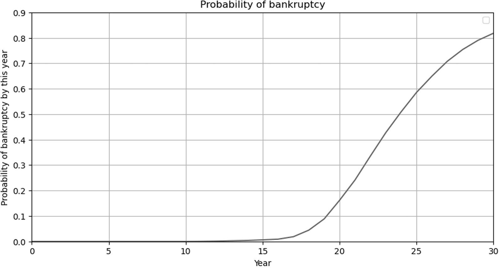


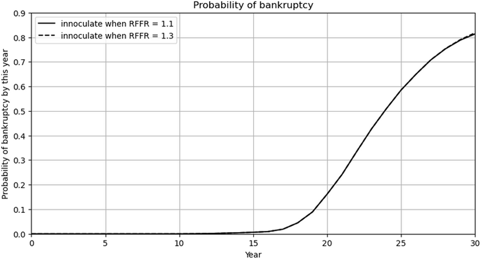





 Open access

