1 Introduction
Robust zonal jets and large-scale coherent vortices are a common feature of the turbulent state in planetary atmospheres and the Earth’s ocean (Ingersoll Reference Ingersoll1990; Maximenko, Bang & Sasaki Reference Maximenko, Bang and Sasaki2005; Chelton et al.
Reference Chelton, Schlax, Samelson and deSzoeke2007; Galperin et al.
Reference Galperin, Young, Sukoriansky, Dikovskaya, Read, Lancaster and Armstrong2014). In order to understand the process of turbulence self-organization into these large-scale structures, simplified theoretical models containing the relevant dynamics have been studied for some years now. One of the simplest models that has been widely studied is barotropic
 $\unicode[STIX]{x1D6FD}$
-plane turbulence (Rhines Reference Rhines1975; Vallis & Maltrud Reference Vallis and Maltrud1993). Following theoretical predictions by Farrell & Ioannou (Reference Farrell and Ioannou2007), recent direct numerical simulations of forced–dissipative barotropic turbulence on a
 $\unicode[STIX]{x1D6FD}$
-plane indicated that large-scale coherent flows emerge through a symmetry-breaking bifurcation of the turbulent flow: as the dissipation or the turbulence intensity varies, the homogeneity of the flow is broken by the spontaneous emergence of zonal jets and large-scale waves, and these large-scale structures are supported at finite amplitude by the turbulent eddies through shear straining (Srinivasan & Young Reference Srinivasan and Young2012; Bakas & Ioannou Reference Bakas and Ioannou2013a
; Constantinou, Farrell & Ioannou Reference Constantinou, Farrell and Ioannou2014a
). A recent extension of the barotropic studies to a stratified two-layer
 $\unicode[STIX]{x1D6FD}$
-plane setting without any imposed mean temperature gradient, has indicated that the jets in regions of reduced dissipation assume a universal barotropic structure (Farrell & Ioannou Reference Farrell and Ioannou2017). In this work, we extend the analytic results from the barotropic set-up to stratified two-layer flows and provide the theoretical arguments that address this finding by answering the following question: in the absence of any imposed mean temperature gradient can externally forced turbulence in a two-layer stratified flow support turbulent equilibria with large-scale baroclinic coherent flows sustained at finite amplitude? Or are the large-scale flows that emerge necessarily barotropic?
To address the emergence of large-scale structure as a bifurcation, a new point of view was recently advanced. Through analysis of the statistical state dynamics (SSD) of the flow, that is of the dynamics that governs the evolution of the flow statistics, a new type of collective instability was revealed and it was proposed that emergence of large-scale structure resulted from this symmetry-breaking instability (Farrell & Ioannou Reference Farrell and Ioannou2003, Reference Farrell and Ioannou2007; Srinivasan & Young Reference Srinivasan and Young2012; Bakas & Ioannou Reference Bakas and Ioannou2013a ; Parker & Krommes Reference Parker and Krommes2013, Reference Parker and Krommes2014). Although these instabilities manifest in single realizations of the flow, their analytical representation requires a statistical framework. The reason is that the cooperative phenomena at play involve Reynolds stresses with large fluctuations. However, it is only the residual statistical mean of the stresses that influences the mean flow coherently, which then modifies the statistics of the distribution of the turbulent eddies. The stability of the large-scale structures is therefore governed by the mean of these complex interactions and as a result, a statistical framework is required in order to analytically express this dynamics.
Analysis of the SSD and the resulting instability is only possible through a closure assumption for the dynamics, as a straightforward calculation leads to an infinite hierarchy of equations for the moments and is therefore intractable (Hopf Reference Hopf1952; Kraichnan Reference Kraichnan1964). There is now a large number of studies of barotropic turbulence (Farrell & Ioannou Reference Farrell and Ioannou2007; Marston Reference Marston2010; Srinivasan & Young Reference Srinivasan and Young2012), shallow-water turbulence (Farrell & Ioannou Reference Farrell and Ioannou2009a ), baroclinic turbulence (DelSole Reference DelSole1996; Farrell & Ioannou Reference Farrell and Ioannou2008, Reference Farrell, Ioannou, Galperin and Read2019), turbulence in pipe flows (Constantinou et al. Reference Constantinou, Lozano-Durán, Nikolaidis, Farrell, Ioannou and Jiménez2014b ; Farrell et al. Reference Farrell, Ioannou, Jiménez, Constantinou, Lozano-Durán and Nikolaidis2016; Farrell, Gayme & Ioannou Reference Farrell, Gayme and Ioannou2017), turbulence in convectively unstable flows (Fitzgerald & Farrell Reference Fitzgerald and Farrell2014; Ait-Chaalal et al. Reference Ait-Chaalal, Schneider, Meyer and Marston2016), turbulence in stably stratified flows (Fitzgerald & Farrell Reference Fitzgerald and Farrell2018) and turbulence in plasma and astrophysical flows (Farrell & Ioannou Reference Farrell and Ioannou2009b ; Tobias, Dagon & Marston Reference Tobias, Dagon and Marston2011; Parker & Krommes Reference Parker and Krommes2013; Constantinou & Parker Reference Constantinou and Parker2018) providing evidence that whenever there is a coherent flow coexisting with the turbulent field, the SSD can be accurately captured by a second-order closure. Such closures of the SSD are either referred to as stochastic structural stability theory (S3T) (Farrell & Ioannou Reference Farrell and Ioannou2003) or second-order cumulant expansion (CE2) (Marston, Conover & Schneider Reference Marston, Conover and Schneider2008).
At first sight the success of a second-order closure is surprising. Consider for example the case of zonal jets supported by barotropic turbulence. The question is whether the quasi-linear eddy-mean flow interaction, which captures shearing of the eddies by the jet, dominates the eddy–eddy interactions that are represented in the higher-order cumulants. Close to the bifurcation point of jet emergence, the mean-flow shear is infinitesimal and presumably the eddy–eddy interactions dominate and the quasi-linear interaction is presumed inadequate to form jets (Srinivasan & Young Reference Srinivasan and Young2012; Frishman & Herbert Reference Frishman and Herbert2018). Also, in highly supercritical regimes and in the limit of high turbulence intensity the eddy–eddy interactions may dominate and the turbulence may become strongly diffusive (Held & Larichev Reference Held and Larichev1996). However, recent studies have provided evidence that the S3T dynamics is dominant both at the bifurcation point and at reasonably high supercriticalities.
Close to the bifurcation point of jet emergence, a second-order closure was shown to be extremely accurate if the dynamics of coherent large-scale waves that significantly influence the flow is suppressed (Constantinou et al. Reference Constantinou, Farrell and Ioannou2014a ) or is accounted for Bakas & Ioannou (Reference Bakas and Ioannou2013a ). In addition, Bakas & Ioannou (Reference Bakas and Ioannou2013b ) and Bakas, Constantinou & Ioannou (Reference Bakas, Constantinou and Ioannou2015) studied in detail the eddy-mean-flow dynamics underlying jet formation. They have shown that close to the bifurcation, when mean flows are very weak and the eddies are dissipated before they are sheared over by the jet, the mean induced fluxes are up-gradient, leading to a positive feedback loop and to exponential growth of the mean jet. It is precisely the existence of this mean feedback of the Reynolds stresses that underlies the exponential instability and overpowers over time the fluctuations leading to the emergence of large-scale structure in single realizations of the flow, in accordance with the predictions of S3T theory.
The regime far from the bifurcation points is characterized by the zonostrophic parameter
 $R_{\unicode[STIX]{x1D6FD}}$
, that measures the ratio of the Rhines scale over the scale where the isotropic energy cascade gets anisotropized by
 $\unicode[STIX]{x1D6FD}$
(Galperin et al.
Reference Galperin, Sukoriansky, Dikovskaya, Read, Yamazaki and Wordsworth2006). The strongly nonlinear regime, referred to as zonostrophic, ensues when
 $R_{\unicode[STIX]{x1D6FD}}\gtrsim 2$
(Galperin et al.
Reference Galperin, Young, Sukoriansky, Dikovskaya, Read, Lancaster and Armstrong2014). Bakas & Ioannou (Reference Bakas, Ioannou, Galperin and Read2019) performed numerical experiments within the zonostrophic regime at
 $R_{\unicode[STIX]{x1D6FD}}=2.5$
and demonstrated that the scale of the emergent structures is well captured by a second-order closure despite some quantitative differences in the intensity of the flows. This demonstrates that, even though the eddy–eddy interactions are not negligible and may contribute to added eddy diffusion in the mean-flow dynamics, they do not affect the S3T collective mechanisms that support the large-scale flows. Scott & Dritschel (Reference Scott and Dritschel2012) performed simulations at even higher values of
 $R_{\unicode[STIX]{x1D6FD}}$
and demonstrated that well-formed potential vorticity (PV) staircases arise when
 $R_{\unicode[STIX]{x1D6FD}}\geqslant 10$
. The accuracy of S3T dynamics in the PV staircase regime at these values of
 $R_{\unicode[STIX]{x1D6FD}}$
has not been checked yet.
As discussed above, S3T has the important advantage that it allows for the analytic treatment of the turbulence–mean-flow instabilities and can lead to a more comprehensive understanding of turbulent bifurcations. For barotropic
 $\unicode[STIX]{x1D6FD}$
-plane turbulence it was shown that jets (Farrell & Ioannou Reference Farrell and Ioannou2007; Srinivasan & Young Reference Srinivasan and Young2012) and large-scale waves (Bakas & Ioannou Reference Bakas and Ioannou2014) emerge as the statistical equilibrium of homogeneous turbulence becomes unstable. This instability, was shown to be the generalization of modulational instability (Connaughton et al.
Reference Connaughton, Nadiga, Nazarenko and Quinn2010) in stochastically forced dissipative flows (Bakas et al.
Reference Bakas, Constantinou and Ioannou2015; Parker & Krommes Reference Parker, Krommes, Galperin and Read2015). In this work, we undertake the task of presenting the analytical S3T theory for a stratified fluid on a
 $\unicode[STIX]{x1D6FD}$
-plane addressing the following question: what type of large-scale flows emerge and are sustained at finite amplitude in a turbulent stratified atmosphere that is homogeneous?
We use a two-layer model on a
 $\unicode[STIX]{x1D6FD}$
-plane that on the one hand allows analytic treatment of the dynamics and numerical integration of the high-dimensional SSD of the flow and, on the other hand, it is a model for both the barotropic and the first baroclinic mode of a fluid of arbitrary depth and, therefore, it is the simplest model that can address whether the dynamics favours formation of large-scale structures that are deep or shallow. We choose to maintain this turbulent field in the simplest manner by introducing (i) a homogeneous and isotropic stochastic excitation that drives the turbulence and (ii) equal linear dissipation of potential vorticity in both layers. The reason for this perfectly symmetric setting is that we want to address whether coherent barotropic or baroclinic flows can arise inherently from turbulence self-organization dynamics rather than through an asymmetric damping between the two layers or through a mean baroclinic shear. That is, we would like to address whether the intrinsic dynamics favours the establishment of arbitrarily deep barotropic coherent structures or not. We first present direct numerical simulations of the turbulent flow that demonstrate the regime transitions in the flow and identify the scales and characteristics of the emergent structures. We then derive the SSD of the flow under a second-order closure with the assumption that the average for defining the statistical moments is coarse graining over fast time scales. We address the instability of the homogeneous equilibrium of the SSD for a wide range of parameters and the properties of the unstable modes that represent the emerging structures. We then study the equilibration of the structure-forming instability, the characteristics of the coherent structures supported at finite amplitude and compare the predictions of the theory to the direct numerical simulations of the turbulent flow, showcasing its validity. We finally discuss the implications of our results for the large-scale structures in planetary flows.
2 Numerical simulations of turbulent flow
Consider a quasi-geostrophic baroclinic two-layer fluid on an infinite
 $\unicode[STIX]{x1D6FD}$
-plane. The upper and lower layers are denoted with subscripts 1 and 2, have equal depth,
 $H/2$
, and densities
 $\unicode[STIX]{x1D70C}_{1}$
and
 $\unicode[STIX]{x1D70C}_{2}$
with
 $\unicode[STIX]{x1D70C}_{2}>\unicode[STIX]{x1D70C}_{1}$
. The quasi-geostrophic dynamics governing the evolution of the barotropic
 $\tilde{\unicode[STIX]{x1D713}}=(\unicode[STIX]{x1D713}_{1}+\unicode[STIX]{x1D713}_{2})/2$
and the baroclinic
 $\tilde{\unicode[STIX]{x1D703}}=(\unicode[STIX]{x1D713}_{1}-\unicode[STIX]{x1D713}_{2})/2$
streamfunction is:
 $$\begin{eqnarray}\displaystyle & \unicode[STIX]{x2202}_{\tilde{t}}\tilde{\unicode[STIX]{x1D701}}+J(\tilde{\unicode[STIX]{x1D713}},\tilde{\unicode[STIX]{x1D701}})+J(\tilde{\unicode[STIX]{x1D703}},\tilde{\unicode[STIX]{x1D6E5}}\tilde{\unicode[STIX]{x1D703}})+\tilde{\unicode[STIX]{x1D6FD}}\unicode[STIX]{x2202}_{\tilde{x}}\tilde{\unicode[STIX]{x1D713}}=-\tilde{r}\tilde{\unicode[STIX]{x1D701}}+\tilde{\unicode[STIX]{x1D709}}^{\unicode[STIX]{x1D713}}, & \displaystyle\end{eqnarray}$$
 $$\begin{eqnarray}\displaystyle & \unicode[STIX]{x2202}_{\tilde{t}}\tilde{\unicode[STIX]{x1D702}}+J(\tilde{\unicode[STIX]{x1D713}},\tilde{\unicode[STIX]{x1D702}})+J(\tilde{\unicode[STIX]{x1D703}},\tilde{\unicode[STIX]{x1D701}})+\tilde{\unicode[STIX]{x1D6FD}}\unicode[STIX]{x2202}_{\tilde{x}}\tilde{\unicode[STIX]{x1D703}}=-\tilde{r}\tilde{\unicode[STIX]{x1D702}}+\tilde{\unicode[STIX]{x1D709}}^{\unicode[STIX]{x1D703}}, & \displaystyle\end{eqnarray}$$
where
 $\tilde{\unicode[STIX]{x1D6E5}}\stackrel{\text{def}}{=}\unicode[STIX]{x2202}_{\tilde{x}}^{2}+\unicode[STIX]{x2202}_{{\tilde{y}}}^{2}$
is the horizontal Laplacian,
 $J(f,g)\stackrel{\text{def}}{=}(\unicode[STIX]{x2202}_{\tilde{x}}f)(\unicode[STIX]{x2202}_{{\tilde{y}}}g)-(\unicode[STIX]{x2202}_{{\tilde{y}}}f)(\unicode[STIX]{x2202}_{\tilde{x}}g)$
is the Jacobian,
 $\tilde{\unicode[STIX]{x1D6E5}}_{\unicode[STIX]{x1D706}}\stackrel{\text{def}}{=}\tilde{\unicode[STIX]{x1D6E5}}-2\tilde{\unicode[STIX]{x1D706}}^{2}$
,
 $\tilde{\unicode[STIX]{x1D701}}\stackrel{\text{def}}{=}\tilde{\unicode[STIX]{x1D6E5}}\tilde{\unicode[STIX]{x1D713}}$
is the barotropic vorticity,
 $\tilde{\unicode[STIX]{x1D702}}\stackrel{\text{def}}{=}\tilde{\unicode[STIX]{x1D6E5}}_{\unicode[STIX]{x1D706}}\tilde{\unicode[STIX]{x1D713}}$
,
 $\tilde{x}$
and
 ${\tilde{y}}$
are the coordinates in the zonal and the meridional direction respectively and the tilde denotes dimensional quantities (cf. Cehelsky & Tung Reference Cehelsky and Tung1991). The deformation radius is
 $1/\tilde{\unicode[STIX]{x1D706}}=\sqrt{g^{\prime }(H/2)}/f_{0}$
, where
 $g^{\prime }=2g(\unicode[STIX]{x1D71A}_{1}-\unicode[STIX]{x1D71A}_{2})/(\unicode[STIX]{x1D71A}_{1}+\unicode[STIX]{x1D71A}_{2})$
is the reduced gravity and
 $f_{0}$
is the Coriolis parameter at the centre of the plane,
 $\tilde{\unicode[STIX]{x1D6FD}}$
is the planetary vorticity gradient and
 $\tilde{r}$
is the coefficient of linear damping of potential vorticity.
We do not impose a temperature gradient across the channel, which through thermal wind balance would impose a mean baroclinic shear. Instead of this large-scale forcing, we impose random baroclinic and barotropic potential vorticity sources and sinks, denoted
 $\tilde{\unicode[STIX]{x1D709}}^{\unicode[STIX]{x1D713}}$
and
 $\tilde{\unicode[STIX]{x1D709}}^{\unicode[STIX]{x1D703}}$
respectively. These sources and sinks represent barotropic and baroclinic excitation of the fluid by sub-scale processes or by processes not included in the quasi-geostrophic dynamics such as convection. The random excitation is assumed to have zero mean, to be temporally delta correlated and to be statistically homogeneous in the horizontal. Under these assumptions, the excitations in the upper layer,
 $\tilde{\unicode[STIX]{x1D709}}_{1}(\tilde{\boldsymbol{x}},\tilde{t})$
, and in the lower layer,
 $\tilde{\unicode[STIX]{x1D709}}_{2}(\tilde{\boldsymbol{x}},\tilde{t})$
, have the two-point, two-time covariances:
 $$\begin{eqnarray}\langle \tilde{\unicode[STIX]{x1D709}}_{i}(\tilde{\boldsymbol{x}}_{a},\tilde{t}_{a})\tilde{\unicode[STIX]{x1D709}}_{j}(\tilde{\boldsymbol{x}}_{b},\tilde{t}_{b})\rangle =\langle \tilde{\unicode[STIX]{x1D709}}_{j}(\tilde{\boldsymbol{x}}_{a},\tilde{t}_{a})\tilde{\unicode[STIX]{x1D709}}_{i}(\tilde{\boldsymbol{x}}_{b},\tilde{t}_{b})\rangle =\unicode[STIX]{x1D6FF}(\tilde{t}_{a}-\tilde{t}_{b})\tilde{\unicode[STIX]{x1D6FC}}_{ij}(\tilde{\boldsymbol{x}}_{a}-\tilde{\boldsymbol{x}}_{b}),\quad i,j=1,2,\end{eqnarray}$$
where
 $\langle \,\boldsymbol{\cdot }\,\rangle$
denotes an ensemble average over forcing realizations,
 $\tilde{\boldsymbol{x}}=(\tilde{x},{\tilde{y}})$
, and the subscript denotes two different points a and b. Statistical homogeneity requires that the covariances are symmetric to the exchange of points a and b and to the exchange of the excitation of the two layers. Therefore the functions
 $\tilde{\unicode[STIX]{x1D6FC}}_{ij}$
satisfy:
 $$\begin{eqnarray}\tilde{\unicode[STIX]{x1D6FC}}_{11}=\tilde{\unicode[STIX]{x1D6FC}}_{22}=2\tilde{\unicode[STIX]{x1D6EF}},\quad \tilde{\unicode[STIX]{x1D6FC}}_{12}=\tilde{\unicode[STIX]{x1D6FC}}_{21}=2\tilde{\unicode[STIX]{x1D6EF}}_{12}.\end{eqnarray}$$
An important consequence of this symmetry is that the barotropic
 $\tilde{\unicode[STIX]{x1D709}}^{\unicode[STIX]{x1D713}}=(\tilde{\unicode[STIX]{x1D709}}_{1}+\tilde{\unicode[STIX]{x1D709}}_{2})/2$
and baroclinic
 $\tilde{\unicode[STIX]{x1D709}}^{\unicode[STIX]{x1D703}}=(\tilde{\unicode[STIX]{x1D709}}_{1}-\tilde{\unicode[STIX]{x1D709}}_{2})/2$
excitations are uncorrelated:
 $\langle \tilde{\unicode[STIX]{x1D709}}^{\unicode[STIX]{x1D713}}(\tilde{\boldsymbol{x}}_{a},\tilde{t}_{a})\tilde{\unicode[STIX]{x1D709}}^{\unicode[STIX]{x1D703}}(\tilde{\boldsymbol{x}}_{b},\tilde{t}_{b})\rangle =0$
. The barotropic and baroclinic component covariances of the forcing are:
 $$\begin{eqnarray}\displaystyle & \langle \tilde{\unicode[STIX]{x1D709}}^{\unicode[STIX]{x1D713}}(\tilde{\boldsymbol{x}}_{a},\tilde{t}_{a})\tilde{\unicode[STIX]{x1D709}}^{\unicode[STIX]{x1D713}}(\tilde{\boldsymbol{x}}_{b},\tilde{t}_{b})\rangle =\unicode[STIX]{x1D6FF}(\tilde{t}_{a}-\tilde{t}_{b})[\vphantom{{\dot{W}}}\tilde{\unicode[STIX]{x1D6EF}}(\tilde{\boldsymbol{x}}_{a}-\tilde{\boldsymbol{x}}_{b})+\tilde{\unicode[STIX]{x1D6EF}}_{12}(\tilde{\boldsymbol{x}}_{a}-\tilde{\boldsymbol{x}}_{b})], & \displaystyle\end{eqnarray}$$
 $$\begin{eqnarray}\displaystyle & \langle \tilde{\unicode[STIX]{x1D709}}^{\unicode[STIX]{x1D703}}(\tilde{\boldsymbol{x}}_{a},\tilde{t}_{a})\tilde{\unicode[STIX]{x1D709}}^{\unicode[STIX]{x1D703}}(\tilde{\boldsymbol{x}}_{b},\tilde{t}_{b})\rangle =\unicode[STIX]{x1D6FF}(\tilde{t}_{a}-\tilde{t}_{b})[\vphantom{{\dot{W}}}\tilde{\unicode[STIX]{x1D6EF}}(\tilde{\boldsymbol{x}}_{a}-\tilde{\boldsymbol{x}}_{b})-\tilde{\unicode[STIX]{x1D6EF}}_{12}(\tilde{\boldsymbol{x}}_{a}-\tilde{\boldsymbol{x}}_{b})]. & \displaystyle\end{eqnarray}$$
If we assume a correlation between the layers
 $\tilde{\unicode[STIX]{x1D6EF}}_{12}=p\tilde{\unicode[STIX]{x1D6EF}}$
, positive definiteness of the covariances implies that
 $|p|\leqslant 1$
. We consider three values for
 $p$
that exemplify opposite limits. We consider the value
 $p=1$
which corresponds to the case of imposing the same excitation on the two layers (
 $\tilde{\unicode[STIX]{x1D709}}_{1}=\tilde{\unicode[STIX]{x1D709}}_{2}$
). For this forcing, the baroclinic forcing covariance is zero and represents at first sight the worst (best) case scenario for the emergence of mean flows with strong baroclinic (barotropic) components. In the second case we take the opposite limit of exciting only the baroclinic part of the flow (
 $p=-1$
) by imposing an anti-correlated excitation in the two layers (
 $\tilde{\unicode[STIX]{x1D709}}_{2}=-\tilde{\unicode[STIX]{x1D709}}_{1}$
). This represents the best (worst) case scenario for the emergence of mean flows with strong baroclinic (barotropic) components. Finally we take
 $p=0$
and consider an independent excitation of the two layers
 $\tilde{\unicode[STIX]{x1D6EF}}_{12}=0$
. In that case, the barotropic and baroclinic forcing covariances are equal:
 $$\begin{eqnarray}\langle \tilde{\unicode[STIX]{x1D709}}^{\unicode[STIX]{x1D713}}(\tilde{\boldsymbol{x}}_{a},\tilde{t}_{a})\tilde{\unicode[STIX]{x1D709}}^{\unicode[STIX]{x1D713}}(\tilde{\boldsymbol{x}}_{b},\tilde{t}_{2}b)\rangle =\langle \tilde{\unicode[STIX]{x1D709}}^{\unicode[STIX]{x1D703}}(\tilde{\boldsymbol{x}}_{a},\tilde{t}_{a})\tilde{\unicode[STIX]{x1D709}}^{\unicode[STIX]{x1D703}}(\tilde{\boldsymbol{x}}_{b},\tilde{t}_{b})\rangle =\unicode[STIX]{x1D6FF}(\tilde{t}_{a}-\tilde{t}_{b})\tilde{\unicode[STIX]{x1D6EF}}(\tilde{\boldsymbol{x}}_{a}-\tilde{\boldsymbol{x}}_{b}).\end{eqnarray}$$
In this work we address the following questions:
(i) For a given spatial structure of the homogeneous forcing
 $\unicode[STIX]{x1D6EF}$
, do any coherent structures with scales different than the ones we directly excite emerge in the flow and what are their characteristics? We are particularly interested in whether the structures that appear are baroclinic or necessarily barotropic.
(ii) Can we develop a theory that is able to explain the emergence of coherent structures and predict their characteristics?

To address the first question, we consider (2.1)–(2.2) in a doubly periodic channel of size
 $2\unicode[STIX]{x03C0}\times 2\unicode[STIX]{x03C0}$
and integrate the equations using a pseudo-spectral code and a fourth-order Runge–Kutta time stepping scheme. For the spatial structure of the excitation, we assume that the forcing injects energy in a thin ring in wavenumber space that has radius
 $\tilde{k}_{f}$
and width
 $\unicode[STIX]{x0394}\tilde{k}_{f}$
(Lilly Reference Lilly1969). The power spectrum of the spatial covariance of the forcing is:
 $$\begin{eqnarray}\hat{\unicode[STIX]{x1D6EF}}(\tilde{\boldsymbol{k}})=\mathop{\sum }_{\tilde{k}_{x}}\mathop{\sum }_{\tilde{k}_{y}}\tilde{\unicode[STIX]{x1D6EF}}(\tilde{\boldsymbol{x}}_{a}-\tilde{\boldsymbol{x}}_{b})\text{e}^{-\text{i}\tilde{\boldsymbol{k}}\boldsymbol{\cdot }(\tilde{\boldsymbol{x}}_{a}-\tilde{\boldsymbol{x}}_{b})}=\left\{\begin{array}{@{}ll@{}}a_{f},\quad & \text{for }|\tilde{k}-\tilde{k}_{f}|\leqslant \unicode[STIX]{x0394}\tilde{k}_{f}\\ 0,\quad & \text{for }|\tilde{k}-\tilde{k}_{f}|>\unicode[STIX]{x0394}\tilde{k}_{f},\end{array}\right.\end{eqnarray}$$
where
 $\tilde{\boldsymbol{k}}=(\tilde{k}_{x},\tilde{k}_{y})$
is the wavevector with total wavenumber
 $\tilde{k}=|\tilde{\boldsymbol{k}}|$
and
 $\tilde{k}_{x}$
,
 $\tilde{k}_{y}$
assume integer values. The amplitude
 $$\begin{eqnarray}a_{f}=\frac{\tilde{\unicode[STIX]{x1D700}}\tilde{k}^{2}(\tilde{k}^{2}+2\tilde{\unicode[STIX]{x1D706}}^{2})^{2}}{4(\tilde{k}^{4}+(2+p)\tilde{\unicode[STIX]{x1D706}}^{4}+3\tilde{k}^{2}\tilde{\unicode[STIX]{x1D706}}^{2})\unicode[STIX]{x0394}\tilde{k}_{f}},\end{eqnarray}$$
is chosen so that the forcing injects energy at a rate
 $\tilde{\unicode[STIX]{x1D700}}$
in the flow. We use the modest
 $M=32\times 32$
resolution and the rather low value
 $\tilde{k}_{f}=6$
(
 $\unicode[STIX]{x0394}\tilde{k}_{f}=1$
). The reason is that we would like to explain the phenomena observed in the direct numerical simulations denoted as NL, with the statistical theory to be developed in §§ 3–5 that requires the integration of the high-dimensional covariance matrix (for a grid with
 $M$
points the covariance has dimension
 $2M^{2}$
). However, the low resolution results were compared to higher resolution simulations and there were no significant differences found. In one-layer flows, strong and persistent large-scale flows are produced when the non-dimensional planetary vorticity gradient
 $\unicode[STIX]{x1D6FD}=\tilde{\unicode[STIX]{x1D6FD}}/\tilde{k}_{f}\tilde{r}$
is large (Bakas & Ioannou Reference Bakas and Ioannou2014). Taking into consideration these results we chose
 $\tilde{\unicode[STIX]{x1D6FD}}=60$
and
 $\tilde{r}=0.1$
yielding the non-dimensional value of
 $\unicode[STIX]{x1D6FD}=100$
, which also roughly corresponds to values characteristic of the atmospheres of the outer planets (Bakas & Ioannou Reference Bakas and Ioannou2014).
Previous studies on the emergence of large-scale structures in forced–dissipative turbulence have used two indices to quantify the energy in the emerging large-scale structures. The first is the zonal mean-flow (zmf) index
 $$\begin{eqnarray}\text{zmf}=\frac{\displaystyle \mathop{\sum }_{\tilde{k}_{y}:\tilde{k}_{y}<\tilde{k}_{f}-\unicode[STIX]{x0394}\tilde{k}_{f}}\hat{E}(\tilde{k}_{x}=0,\tilde{k}_{y})}{\displaystyle \mathop{\sum }_{\tilde{k}_{x}\tilde{k}_{y}}\hat{E}(\tilde{k}_{x},\tilde{k}_{y})},\end{eqnarray}$$
with
 $$\begin{eqnarray}\hat{E}(\tilde{k}_{x},\tilde{k}_{y})=\lim _{T\rightarrow \infty }\frac{1}{T}\int _{0}^{T}\tilde{k}^{2}(|\hat{\unicode[STIX]{x1D713}}|^{2}+|\hat{\unicode[STIX]{x1D703}}|^{2})\,\text{d}\tilde{t},\end{eqnarray}$$
the time averaged kinetic energy of the flow at wavenumbers
 $(\tilde{k}_{x},\tilde{k}_{y})$
. The zmf index determines the ratio of the energy of the zonal component of the flow to the total energy of the flow and was used by Srinivasan & Young (Reference Srinivasan and Young2012) to study the emergence of jets in barotropic turbulence. The second is the non-zonal mean-flow (nzmf) index:
 $$\begin{eqnarray}\text{nzmf}=\frac{\displaystyle \mathop{\sum }_{\tilde{k}_{x}\tilde{k}_{y}:\tilde{k}<\tilde{k}_{f}-\unicode[STIX]{x0394}\tilde{k}_{f}}\hat{E}(\tilde{k}_{x}\neq 0,\tilde{k}_{y})}{\displaystyle \mathop{\sum }_{\tilde{k}_{x}\tilde{k}_{y}}\hat{E}(\tilde{k}_{x},\tilde{k}_{y})},\end{eqnarray}$$
that determines the ratio of the energy in waves with scales larger than the scale of the forcing (
 $\tilde{k}<\tilde{k}_{f}$
) to the total energy in the flow and was used by Bakas & Ioannou (Reference Bakas and Ioannou2013a
) to study the emergence of large-scale waves. If the large-scale waves that emerge are coherent, then these indices quantify their amplitude.
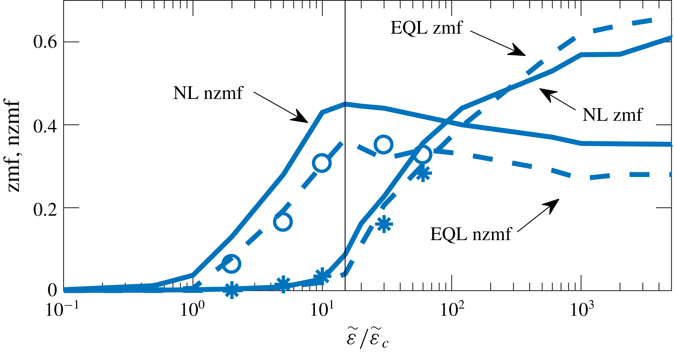
The zmf and nzmf indices defined in (2.10) and (2.12) respectively, as a function of the energy input rate
 $\tilde{\unicode[STIX]{x1D700}}$
for the fully nonlinear (NL) integrations (solid lines), the ensemble quasi-linear (EQL) integrations (dashed lines) and the S3T simulations (open circles for the nzmf and stars for the zmf index). The latter two are discussed in §§ 5 and 6. The critical energy input rate
 $\tilde{\unicode[STIX]{x1D700}}_{c}$
for which the homogeneous state becomes unstable is calculated from the S3T stability analysis (in § 4) and the critical energy input rate
 $\tilde{\unicode[STIX]{x1D700}}_{nl}$
for which the travelling wave states become unstable with respect to zonal perturbations is shown by the vertical thin line (see § 5). The parameters values are
 $\tilde{\unicode[STIX]{x1D6FD}}=60$
,
 $\tilde{k}_{f}=6$
,
 $\unicode[STIX]{x0394}\tilde{k}_{f}=1$
,
 $\tilde{r}=0.1$
,
 $\tilde{\unicode[STIX]{x1D706}}=\tilde{k}_{f}$
and the forcing between the two layers is uncorrelated (
 $p=0$
).

Figure 1 shows the dependence of the nzmf and zmf indices on the energy input rate
 $\tilde{\unicode[STIX]{x1D700}}$
for NL simulations with a Rossby radius of deformation comparable to the forcing scale
 $\tilde{\unicode[STIX]{x1D706}}=\tilde{k}_{f}$
and an uncorrelated forcing between the two layers (
 $p=0$
). We observe that for
 $\tilde{\unicode[STIX]{x1D700}}$
lower than the critical value
 $\tilde{\unicode[STIX]{x1D700}}_{c}$
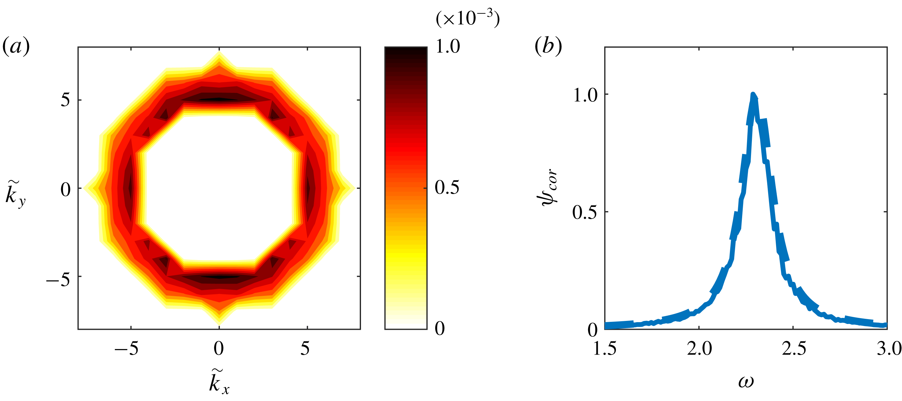
, which will be theoretically predicted in § 4, there are no large-scale structures in the flow. This can also be verified by the kinetic energy power spectra of the barotropic part of the flow shown in figure 2(a), as the spectra contain only the ring of forced wavenumbers. Therefore the flow is dominated by the directly forced waves that obey the Rossby wave dispersion but are phase incoherent. To quantify this we calculate the ensemble mean of the frequency power spectrum of the streamfunction field at wavenumber
 $(\tilde{k}_{x},\tilde{k}_{y})$
:
 $$\begin{eqnarray}\unicode[STIX]{x1D713}_{cor}=\langle |\hat{\unicode[STIX]{x1D713}}(\tilde{k}_{x},\tilde{k}_{y},\tilde{\unicode[STIX]{x1D714}})|^{2}\rangle ,\end{eqnarray}$$
where
 $$\begin{eqnarray}\hat{\unicode[STIX]{x1D713}}(\tilde{k}_{x},\tilde{k}_{y},\tilde{\unicode[STIX]{x1D714}})=\int \mathop{\sum }_{\tilde{x},{\tilde{y}}}\unicode[STIX]{x1D713}(\tilde{x},{\tilde{y}},\tilde{t})\text{e}^{-\text{i}\tilde{\boldsymbol{k}}\boldsymbol{\cdot }\tilde{\boldsymbol{x}}-\text{i}\tilde{\unicode[STIX]{x1D714}}\tilde{t}}\,\text{d}\tilde{t},\end{eqnarray}$$
for the barotropic part of the flow. Similarly we calculate
 $\unicode[STIX]{x1D703}_{cor}$
for the baroclinic part. Travelling waves manifest as peaks at specific frequencies with phase coherence over times proportional to the inverse of the half-width of their resonant peak. We consider that the structure that emerges is phase coherent when its coherence time exceeds the dissipation time scale, which is the time over which a linear wave stochastically excited by white noise remains coherent. Figure 2(b) shows the barotropic frequency power spectrum
 $\unicode[STIX]{x1D713}_{cor}$
for one of the waves in the forced ring with wavenumbers
 $(\tilde{k}_{xr},\tilde{k}_{yr})=(1,5)$
. The frequency power spectrum peaks at the Rossby wave frequency
 $\unicode[STIX]{x1D714}_{r}=\tilde{\unicode[STIX]{x1D6FD}}\tilde{k}_{xr}/(\tilde{k}_{xr}^{2}+\tilde{k}_{yr}^{2})$
, while comparison of its half-width with the corresponding half-width of the power spectrum of stochastically forced linear Rossby waves with the same wavenumbers shows that the coherence time for these waves is the dissipation time scale.
(a) Long-time average of the kinetic energy power spectra of the barotropic part of the turbulent flow at statistical equilibrium obtained from an NL simulation at
 $\tilde{\unicode[STIX]{x1D700}}=\tilde{\unicode[STIX]{x1D700}}_{c}/2$
. (b) The ensemble mean frequency power spectrum
 $\unicode[STIX]{x1D713}_{cor}$
(defined in (2.13)) for the
 $\tilde{\boldsymbol{k}}=(1,5)$
barotropic wave. The frequency power spectrum is normalized to unit maximum amplitude for illustration purposes. The corresponding normalized
 $\unicode[STIX]{x1D713}_{cor}$
for linear Rossby waves with the same wavenumber and stochastically forced by white noise is also shown (dashed lines) for comparison.

The rapid increase in the nzmf index for
 $\tilde{\unicode[STIX]{x1D700}}>\tilde{\unicode[STIX]{x1D700}}_{c}$
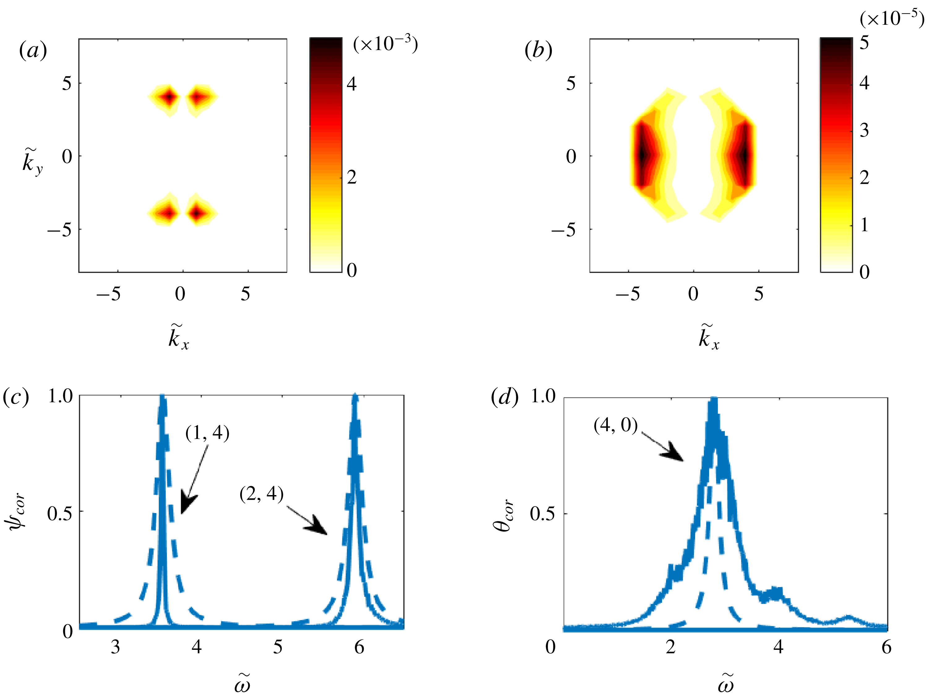
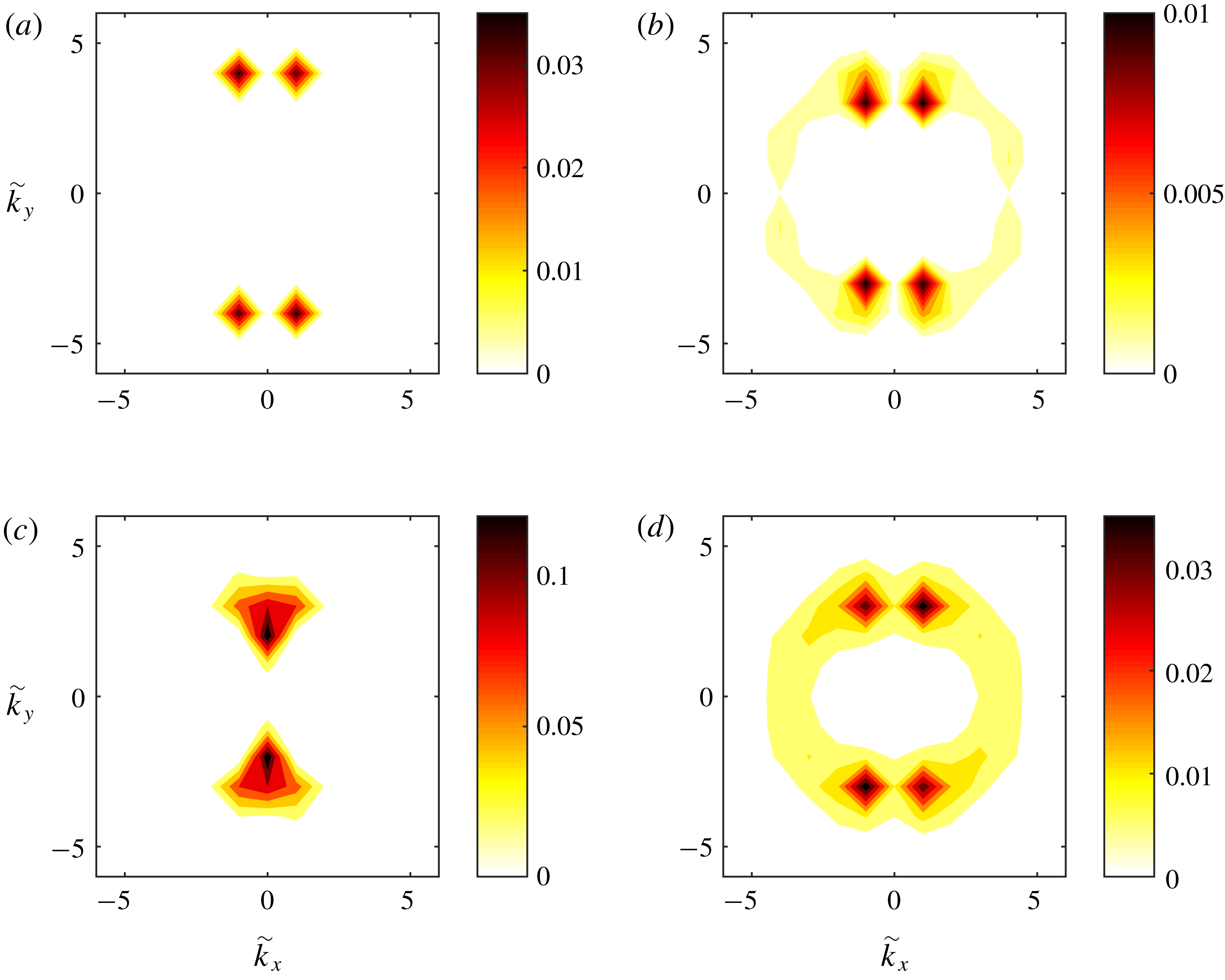
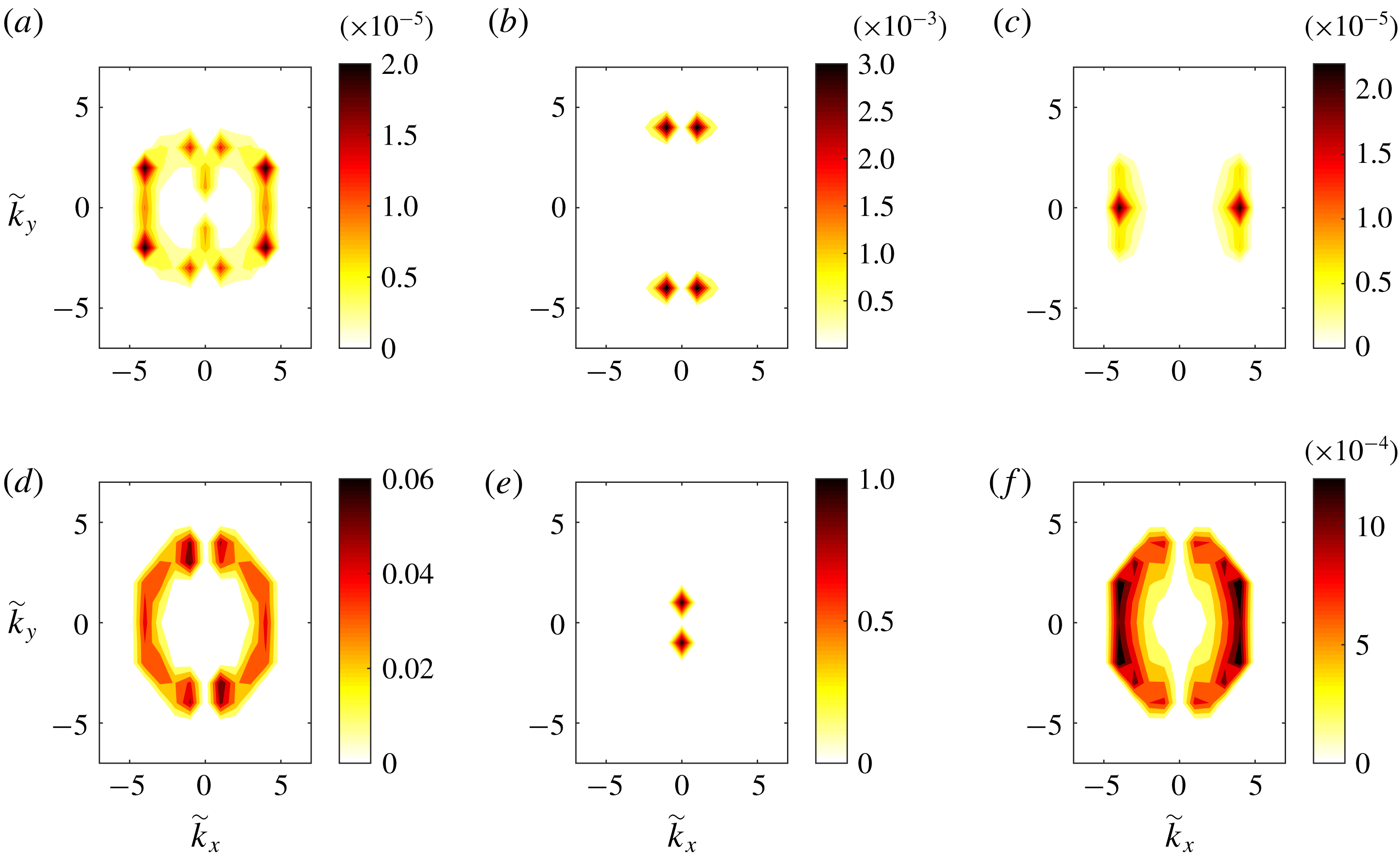
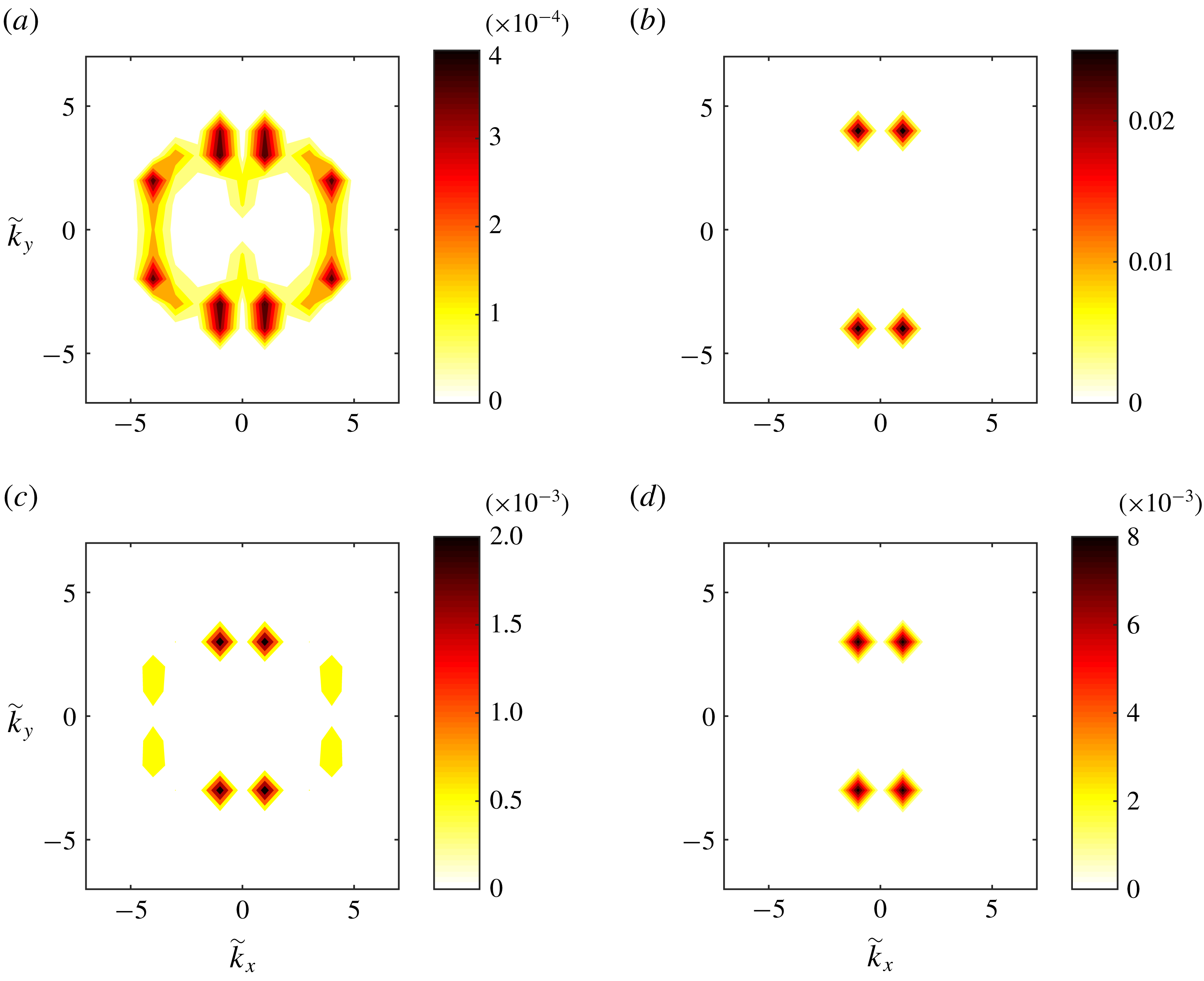
shown in figure 1, signifies the emergence of large-scale waves in the flow. The scales of the waves are shown in figure 3 which illustrates the kinetic energy power spectra at statistical equilibrium for
 $\tilde{\unicode[STIX]{x1D700}}=2\tilde{\unicode[STIX]{x1D700}}_{c}$
. We observe that the kinetic energy of the barotropic part of the flow (cf. figure 3
a) peaks at wavenumbers
 $(|\tilde{k}_{x}|,|\tilde{k}_{y}|)=(1,4)$
and
 $(|\tilde{k}_{x}|,|\tilde{k}_{y}|)=(2,4)$
. In figure 3(c) we plot the barotropic frequency power spectrum
 $\unicode[STIX]{x1D713}_{cor}$
for the two
 $\tilde{\boldsymbol{k}}=(1,4)$
and
 $\tilde{\boldsymbol{k}}=(2,4)$
dominant barotropic structures and compare them with the corresponding power spectrum of stochastically forced linear Rossby waves with the same wavenumbers. We observe that both the
 $(1,4)$
and the
 $(2,4)$
waves remain phase coherent (over six and two dissipation time scales respectively) and also satisfy to a good approximation the Rossby wave dispersion as
 $\unicode[STIX]{x1D713}_{cor}$
peaks at the corresponding Rossby wave frequencies for both wavevectors. In contrast, the baroclinic component of the flow is very weak compared to the barotropic part (cf. figure 3
b) and the emergent structures have an incoherent baroclinic part. For example, the wave with
 $\tilde{\boldsymbol{k}}=(4,0)$
that achieves maximum kinetic energy for the baroclinic component remains phase coherent for very short times (shorter than
 $1/\tilde{r}$
) as revealed by its frequency power spectrum
 $\unicode[STIX]{x1D703}_{cor}$
that is shown in figure 3(d). We can therefore conclude that large-scale, phase coherent, barotropic Rossby waves emerge in the flow for
 $\tilde{\unicode[STIX]{x1D700}}>\tilde{\unicode[STIX]{x1D700}}_{c}$
. For larger energy input rates, the energy in these large-scale waves increases (increasing nzmf index in figure 1) as well as the scales of the dominant waves.
(a,b) Long-time average of the kinetic energy power spectra of the (a) barotropic and (b) baroclinic part of the turbulent flow at statistical equilibrium, obtained from an NL simulation at
 $\tilde{\unicode[STIX]{x1D700}}=2\tilde{\unicode[STIX]{x1D700}}_{c}$
. Shown are the spectra in the region in wavenumber space inside the forced ring. (c) The ensemble mean frequency power spectrum
 $\unicode[STIX]{x1D713}_{cor}$
for the two
 $\tilde{\boldsymbol{k}}=(1,4)$
and
 $\tilde{\boldsymbol{k}}=(2,4)$
barotropic waves dominating the kinetic energy power spectra in (a). The frequency power spectrum is normalized to unit maximum amplitude for illustration purposes (as observed in (a) the
 $\tilde{\boldsymbol{k}}=(1,4)$
wave has approximately twice the energy of the
 $\tilde{\boldsymbol{k}}=(2,4)$
wave). (d) The ensemble mean frequency power spectrum
 $\unicode[STIX]{x1D703}_{cor}$
for the
 $\tilde{\boldsymbol{k}}=(4,0)$
baroclinic wave dominating the kinetic energy power spectra in (b). In (c,d) the corresponding normalized
 $\unicode[STIX]{x1D713}_{cor}$
and
 $\unicode[STIX]{x1D703}_{cor}$
for linear Rossby waves with the same wavenumbers and stochastically forced by white noise are also shown (dashed lines) for comparison.

When the energy input rate passes a second threshold
 $\tilde{\unicode[STIX]{x1D700}}_{nl}$
, which will be calculated in § 5, large-scale zonal jets emerge as signified by the increase of the zmf index for
 $\tilde{\unicode[STIX]{x1D700}}>\tilde{\unicode[STIX]{x1D700}}_{nl}$
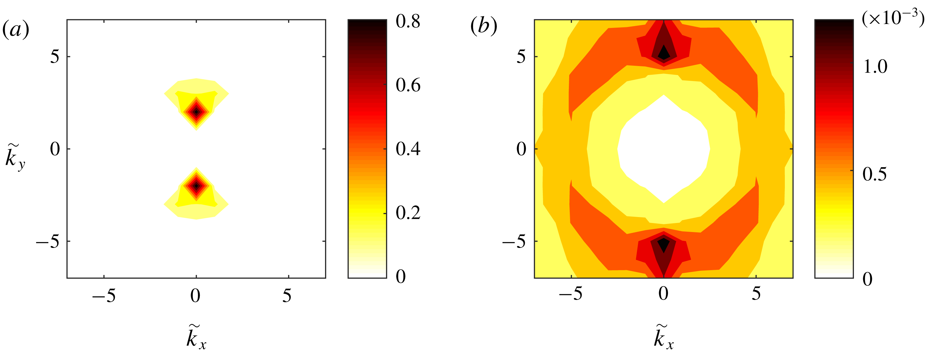
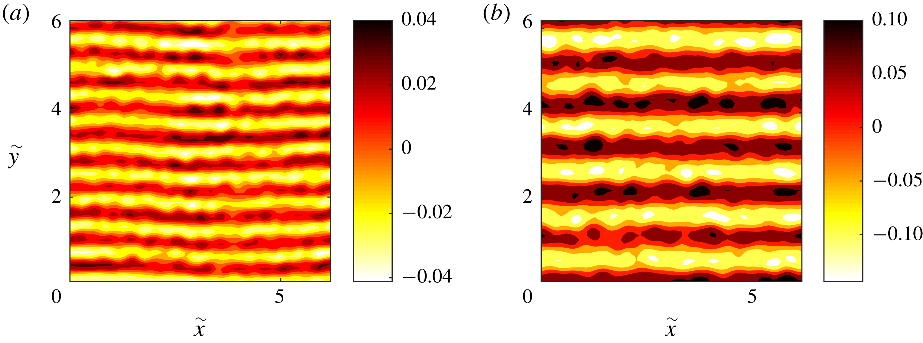
shown in figure 1. The barotropic kinetic energy spectra for
 $\tilde{\unicode[STIX]{x1D700}}=60\tilde{\unicode[STIX]{x1D700}}_{c}$
shown in figure 4(a), reveal that the zonal jet with
 $(|\tilde{k}_{x}|,|\tilde{k}_{y}|)=(0,2)$
dominates the flow, while there is a secondary peak at the wave with
 $(|\tilde{k}_{x}|,|\tilde{k}_{y}|)=(1,3)$
that is phase coherent (not shown). The baroclinic part of the spectrum fills the whole area inside the ring of forced wavenumbers but is three orders of magnitude smaller. As the energy input rate further increases, the energy being pumped into the barotropic zonal jets increases, while the energy of the large-scale barotropic waves decreases (cf. figure 1). The scales of both the jets and the waves also increase. In summary, there are two regime transitions in the flow as the energy input rate of the forcing increases. In the first transition, phase coherent, large-scale Rossby waves emerge and break the homogeneity of the turbulent flow and in the second transition large-scale barotropic zonal jets emerge.
Long-time average of the kinetic energy power spectra of the (a) barotropic and (b) baroclinic part of the turbulent flow at statistical equilibrium obtained for
 $\tilde{\unicode[STIX]{x1D700}}=60\tilde{\unicode[STIX]{x1D700}}_{c}$
.

For lower values of the Rossby radius of deformation
 $\tilde{\unicode[STIX]{x1D706}}$
, the bifurcation diagram is similar with the two regimes of large-scale waves and large-scale jets evident when the energy input rate passes a critical value. However, the structures that dominate the flow have a baroclinic component as well. Figure 5 shows the kinetic energy power spectra for
 $\tilde{\unicode[STIX]{x1D706}}=\tilde{k}_{f}/6$
and two values of the energy input rate above the critical threshold
 $\tilde{\unicode[STIX]{x1D700}}_{c}$
. For low energy input rates (cf. figure 5
a,b), the flow is dominated by a barotropic wave with
 $(|\tilde{k}_{x}|,|\tilde{k}_{y}|)=(1,4)$
and a baroclinic wave with
 $(|\tilde{k}_{x}|,|\tilde{k}_{y}|)=(1,3)$
and an amplitude for the baroclinic streamfunction approximately half of the amplitude of the barotropic streamfunction. Calculation of the frequency power spectra
 $\unicode[STIX]{x1D713}_{cor}$
and
 $\unicode[STIX]{x1D703}_{cor}$
reveals that both of these waves follow the Rossby wave dispersion and remain phase coherent over times longer than the dissipation time scale (not shown).
At larger energy input rates (cf. figure 5
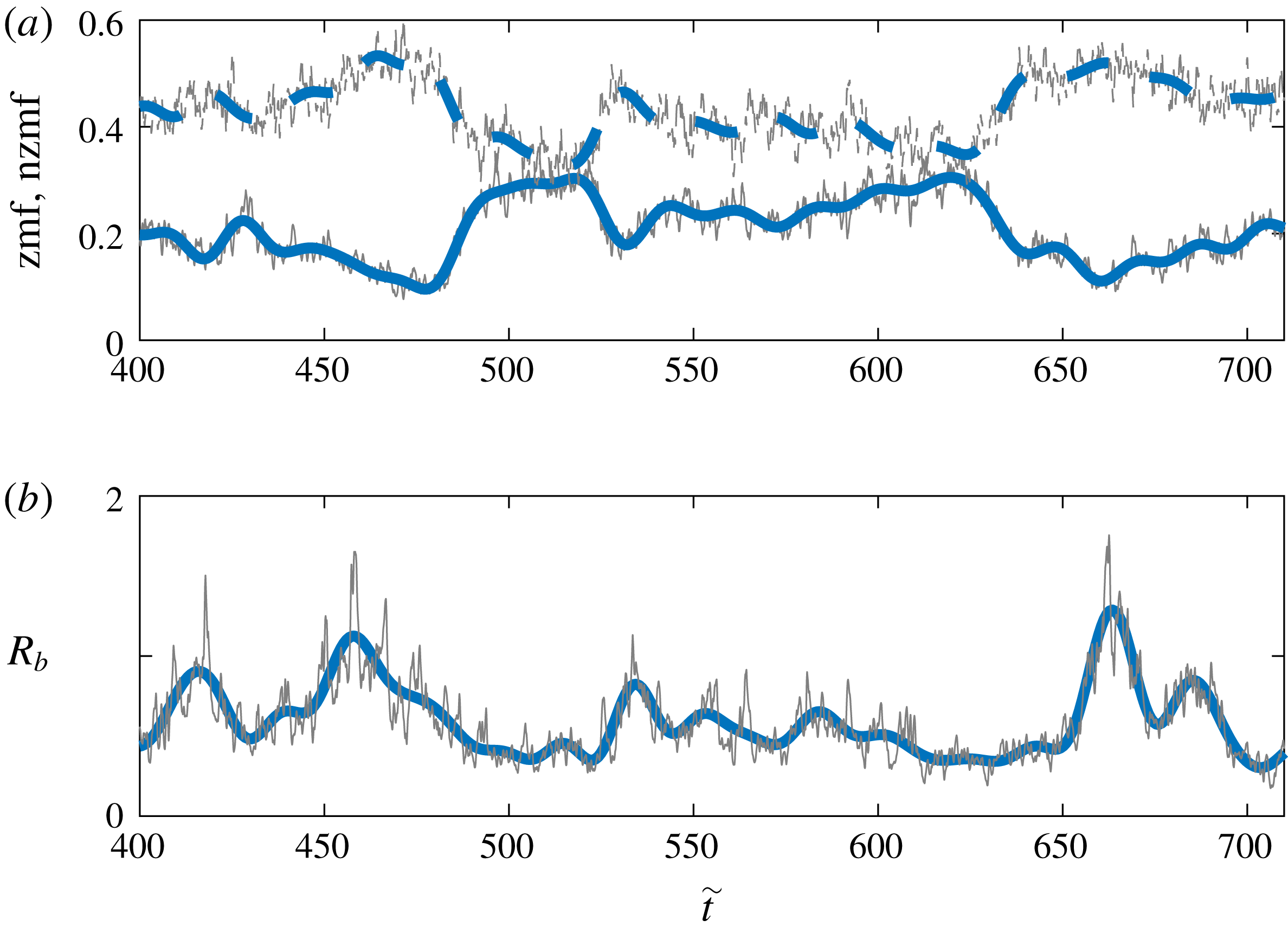
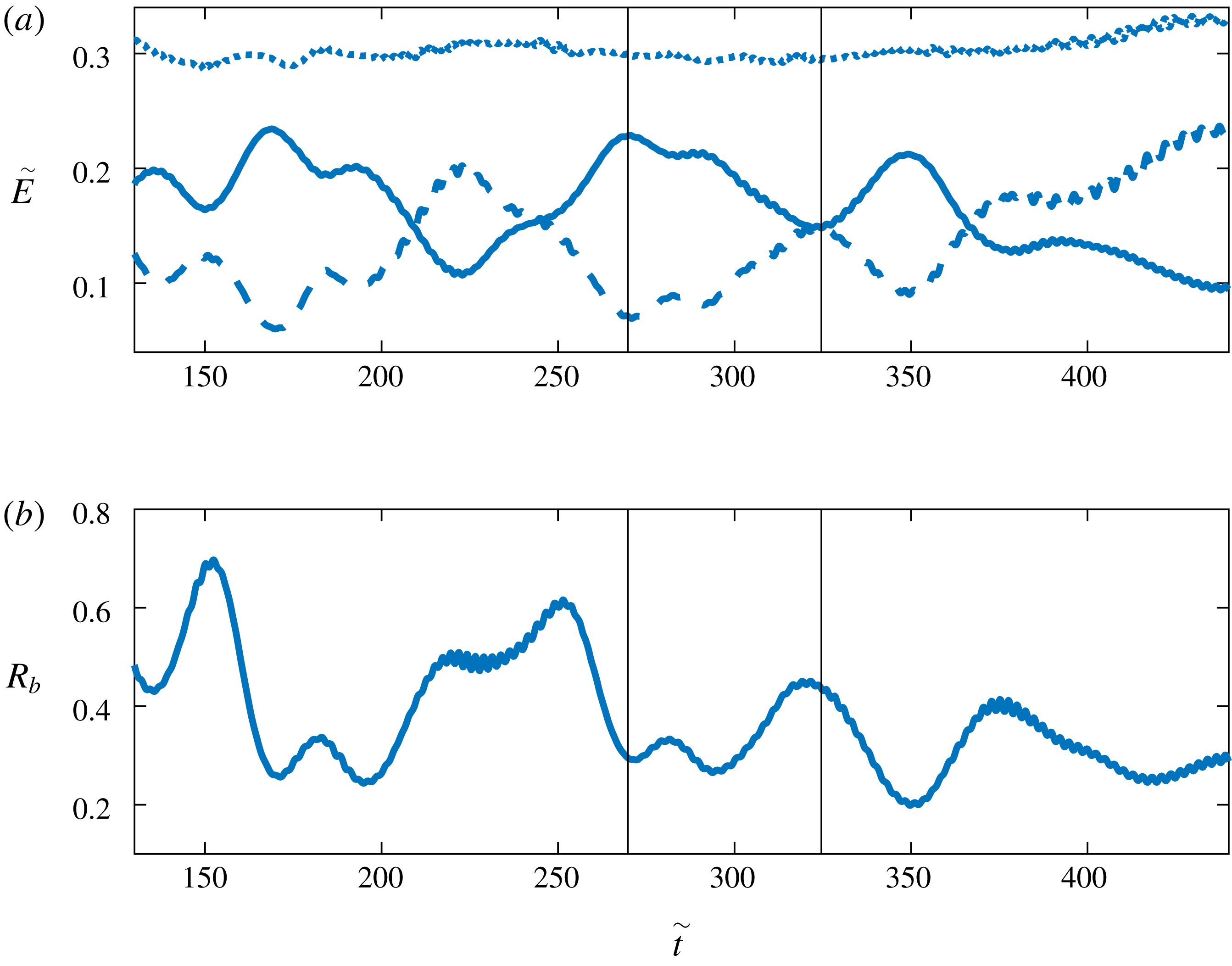
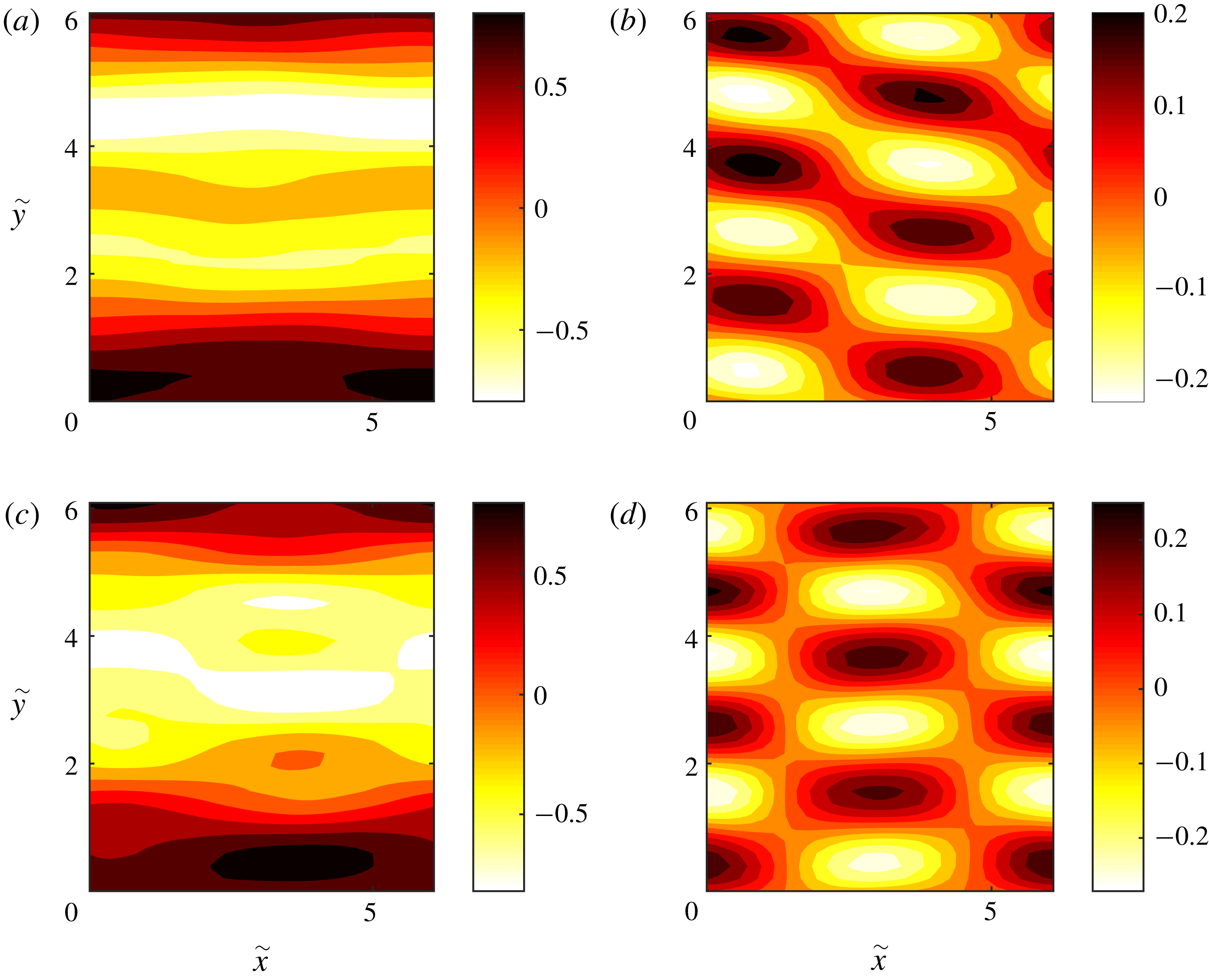
c,d), the flow is dominated by a barotropic jet accompanied by a baroclinic wave. This state was found to exhibit significant variability at long time scales of the order of
 $10/\tilde{r}$
. Figure 6(a) shows the evolution of the zmf and nzmf indices. We observe a low frequency variability of the two indices that are anti-correlated, with time periods of stronger jets/weaker waves and time periods of weaker jets/stronger waves. Similar variability is observed in the baroclinicity measure:
 $$\begin{eqnarray}R_{b}=\frac{\displaystyle \mathop{\sum }_{\tilde{k}_{x},\tilde{k}_{y}}(\tilde{k}^{2}+2\tilde{\unicode[STIX]{x1D706}}^{2})|\hat{\unicode[STIX]{x1D703}}(\tilde{\boldsymbol{k}})|^{2}}{\displaystyle \mathop{\sum }_{\tilde{k}_{x},\tilde{k}_{y}}\tilde{k}^{2}|\hat{\unicode[STIX]{x1D713}}(\tilde{\boldsymbol{k}})|^{2}},\end{eqnarray}$$
that is shown in figure 6(b), where the periods of stronger waves are accompanied by higher values for the flow baroclinicity. Therefore, we observe an energy exchange between the barotropic zonal jet and the large-scale baroclinic wave. For larger energy input rates, the baroclinic part of the flow weakens along with the amplitude of this low frequency variability. As a result, for geophysical flows that are highly supercritical with respect to the structure-forming instability such as the Jovian atmosphere, the baroclinic component of the flow is expected to be very weak.
(a,b) Long-time average of the kinetic energy power spectra of the (a) barotropic and (b) baroclinic part of the turbulent flow at statistical equilibrium for a NL simulation with
 $\tilde{\unicode[STIX]{x1D700}}=10\tilde{\unicode[STIX]{x1D700}}_{c}$
. (c,d) The same as (a,b) but for
 $\tilde{\unicode[STIX]{x1D700}}=40\tilde{\unicode[STIX]{x1D700}}_{c}$
. The deformation radius is
 $\tilde{\unicode[STIX]{x1D706}}=\tilde{k}_{f}/6$
and the rest of the parameter values are the same as in figure 1.

(a) Evolution of the zmf (solid) and nzmf (dashed) indices (thin lines). The thick lines show the low pass filtered time series of the indices. (b) Evolution of the baroclinicity ratio (thin line). The thick line shows a low pass filtered time series of
 $R_{b}$
. The energy input rate is
 $\tilde{\unicode[STIX]{x1D700}}=40\tilde{\unicode[STIX]{x1D700}}_{c}$
, the deformation radius is
 $\tilde{\unicode[STIX]{x1D706}}=\tilde{k}_{f}/6$
and the rest of the parameters are as in figure 1.

We now test the sensitivity of the obtained results to the forcing correlation between the two layers. The barotropic forcing (
 $p=1$
) presents at first sight the worst case scenario for symmetry breaking by baroclinic structures since only barotropic eddies are injected in the flow. However, the regime transitions observed for uncorrelated forcing as well as the characteristics of the emergent structures remain the same. In contrast, the baroclinic forcing (
 $p=-1$
) presents at first sight the worst case scenario for the emergence of barotropic flows. For
 $\tilde{\unicode[STIX]{x1D706}}=\tilde{k}_{f}/6$
and
 $\tilde{\unicode[STIX]{x1D706}}=\tilde{k}_{f}$
the regime transitions are the same as in the case of uncorrelated forcing (
 $p=0$
) and are not shown. The only difference is that the phase coherent barotropic waves that emerge in the case of
 $\tilde{\unicode[STIX]{x1D706}}=\tilde{k}_{f}$
have scales comparable to the forcing scale
 $\tilde{k}_{f}$
. A slightly different picture emerges when energy is injected at scales larger than the deformation radius as the wave regime is absent. For example, when
 $\tilde{\unicode[STIX]{x1D706}}=2\tilde{k}_{f}$
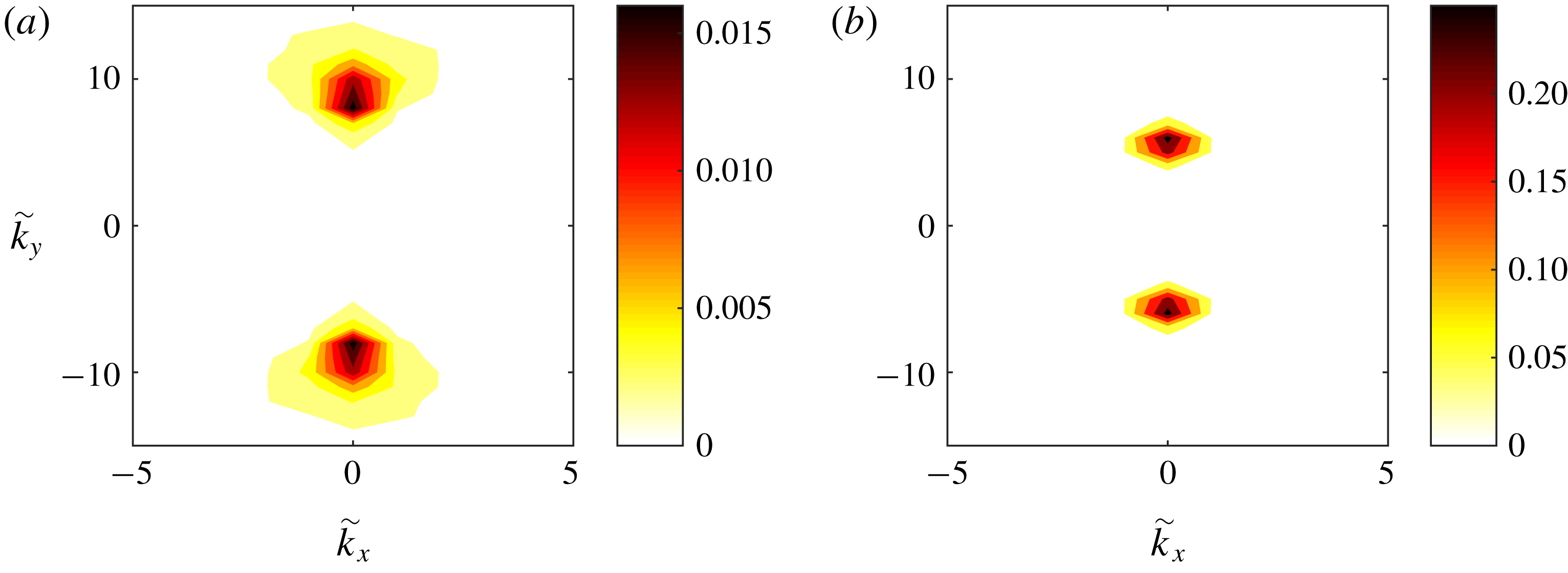
there is only one regime transition in the turbulent flow as the energy input rate of the forcing is increased with the emergence of zonal jets breaking the translational symmetry in the flow. Figure 7 illustrates the kinetic energy power spectrum of the barotropic part for two supercritical values of the energy input rate. For low energy input rates shown in figure 7(a) (
 $\tilde{\unicode[STIX]{x1D700}}=4\tilde{\unicode[STIX]{x1D700}}_{c}$
), the jets have scales comparable to the deformation scale as the power spectra peak at
 $|\tilde{k}_{y}|=3\tilde{\unicode[STIX]{x1D706}}/4$
. For larger energy input rates shown in figure 7(b) the jets obtain larger scales and as the energy input rate is further increased the energy is pumped into larger- and larger-scale jets.
Long-time average of the kinetic energy power spectra of the barotropic part of the turbulent flow at statistical equilibrium for (a)
 $\tilde{\unicode[STIX]{x1D700}}=10\tilde{\unicode[STIX]{x1D700}}_{c}$
and (b)
 $\tilde{\unicode[STIX]{x1D700}}=60\tilde{\unicode[STIX]{x1D700}}_{c}$
. The forcing is baroclinic (
 $p=-1$
),
 $\tilde{\unicode[STIX]{x1D706}}=2\tilde{k}_{f}$
and the rest of the parameter values are the same as in figure 1. These simulations were performed with a
 $64\times 64$
resolution.

To summarize, when the energy injection scale is comparable to the Rossby radius of deformation, the homogeneity of the flow is broken by the emergence of large-scale barotropic waves and large-scale zonal jets as the energy input rate passes certain thresholds. When the energy injection scale is smaller than the Rossby radius of deformation, both barotropic and baroclinic large-scale waves emerge in the flow and for large energy input rates the barotropic part of the flow is zonated and becomes dominant. These results are in general independent of the correlation of the excitation between the two layers with minor exceptions (for example the absence of the wave regime when the energy injection scale is larger than the Rossby radius of deformation). In the following sections we develop a theory that explains the emergence of large-scale flows as a bifurcation and is also able to predict the characteristics of the emergent structures.
3 Stochastic structural stability theory
In order to analyse the transition from a statistically homogeneous to a statistically inhomogeneous turbulent state, we consider the statistical state dynamics (SSD) of the two-layer model (2.1)–(2.2) which comprises the dynamics of the cumulants of the flow. Due to the infinite hierarchy of the resulting equations, this system has to be closed at a certain order through an approximation or assumption. We follow previous studies and consider a second-order closure that is called S3T or CE2 (Farrell & Ioannou Reference Farrell and Ioannou2003; Marston et al. Reference Marston, Conover and Schneider2008). The cumulants are defined by using a proper averaging operator (cf. Monin & Yaglom Reference Monin and Yaglom1973) that captures the emergent large-scale structure (e.g. zonal jet or planetary-scale wave) and additionally satisfies the ergodic property that the second-order cumulants are equal to the ensemble average over forcing realizations under the same first cumulant. In order to address the emergence of both zonal jets and coherent waves in this work, we employ the ensemble average and interpret it as an average over an intermediate time scale which is long compared to the time scale of the evolution of the incoherent flow but short compared to the time scale for the evolution of the mean. Similar assumptions for the average separating fast from slow motions or large-scale from small-scale motions were also made in previous studies (Bernstein & Farrell Reference Bernstein and Farrell2010; Bakas & Ioannou Reference Bakas and Ioannou2014; Constantinou, Farrell & Ioannou Reference Constantinou, Farrell and Ioannou2016; Marston, Chini & Tobias Reference Marston, Chini and Tobias2016; Bouchet, Marston & Tangarife Reference Bouchet, Marston and Tangarife2018).
In order to formulate the theory for the two-layer flow, we first non-dimensionalize (2.1)–(2.2) by choosing the damping relaxation time scale,
 $1/\tilde{r}$
, as the characteristic time scale and the scale of the excitation,
 $1/\tilde{k}_{f}$
, as the characteristic length scale. The non-dimensional variables are:
 $[\unicode[STIX]{x1D701},\unicode[STIX]{x1D702}]=[\tilde{\unicode[STIX]{x1D701}},\tilde{\unicode[STIX]{x1D702}}]/\tilde{r}$
,
 $[\unicode[STIX]{x1D713},\unicode[STIX]{x1D703}]=[\tilde{\unicode[STIX]{x1D713}},\tilde{\unicode[STIX]{x1D703}}]\tilde{k}_{f}^{2}/\tilde{r}$
,
 $[\unicode[STIX]{x1D709}^{\unicode[STIX]{x1D713}},\unicode[STIX]{x1D709}^{\unicode[STIX]{x1D703}}]=[\tilde{\unicode[STIX]{x1D709}}^{\unicode[STIX]{x1D713}},\tilde{\unicode[STIX]{x1D709}}^{\unicode[STIX]{x1D703}}]/\tilde{r}^{2}$
,
 $\unicode[STIX]{x1D700}=\tilde{\unicode[STIX]{x1D700}}\tilde{k}_{f}^{2}/\tilde{r}^{3}$
,
 $\unicode[STIX]{x1D6FD}=\tilde{\unicode[STIX]{x1D6FD}}/(\tilde{k}_{f}\tilde{r})$
,
 $\unicode[STIX]{x1D706}=\tilde{\unicode[STIX]{x1D706}}/\tilde{k}_{f}$
and
 $r=1$
. Thus, the non-dimensional version of (2.1)–(2.2) lacks all tildes and has
 $r=1$
. We also approximate the ring forcing spectrum (2.8) with a forcing covariance that is isotropic and injects energy in a delta ring in wavenumber space of radius 1:
 $$\begin{eqnarray}\hat{\unicode[STIX]{x1D6EF}}(\boldsymbol{k})=\frac{\unicode[STIX]{x1D700}(1+2\unicode[STIX]{x1D706}^{2})^{2}}{2(1+(2+p)\unicode[STIX]{x1D706}^{4}+3\unicode[STIX]{x1D706}^{2})}\unicode[STIX]{x1D6FF}(k-1).\end{eqnarray}$$
Again, the amplitude is chosen to yield an energy injection rate
 $\unicode[STIX]{x1D700}$
.
The first cumulant of the barotropic and baroclinic streamfunctions are
 $\unicode[STIX]{x1D6F9}(\boldsymbol{x},t)\stackrel{\text{def}}{=}\langle \unicode[STIX]{x1D713}\rangle$
and
 $\unicode[STIX]{x1D6E9}(\boldsymbol{x},t)\stackrel{\text{def}}{=}\langle \unicode[STIX]{x1D703}\rangle$
, while the eddy field is denoted with dashes and defined as
 $\unicode[STIX]{x1D713}^{\prime }(\boldsymbol{x},t)=\unicode[STIX]{x1D713}-\langle \unicode[STIX]{x1D713}\rangle$
,
 $\unicode[STIX]{x1D703}^{\prime }(\boldsymbol{x},t)\stackrel{\text{def}}{=}\unicode[STIX]{x1D703}-\langle \unicode[STIX]{x1D703}\rangle$
. In order to derive the S3T system we first derive from (2.1)–(2.2) the equations for the mean and the eddies:
 $$\begin{eqnarray}\displaystyle & \unicode[STIX]{x2202}_{t}Z+J(\unicode[STIX]{x1D6F9},Z)+J(\unicode[STIX]{x1D6E9},\unicode[STIX]{x0394}\unicode[STIX]{x1D6E9})+\unicode[STIX]{x1D6FD}\unicode[STIX]{x2202}_{x}\unicode[STIX]{x1D6F9}=-\langle J(\unicode[STIX]{x1D713}^{\prime },\unicode[STIX]{x1D701}^{\prime })+J(\unicode[STIX]{x1D703}^{\prime },\unicode[STIX]{x0394}\unicode[STIX]{x1D703}^{\prime })\vphantom{{\dot{W}}}\rangle -Z, & \displaystyle\end{eqnarray}$$
 $$\begin{eqnarray}\displaystyle & \unicode[STIX]{x2202}_{t}H+J(\unicode[STIX]{x1D6F9},H)+J(\unicode[STIX]{x1D6E9},Z)+\unicode[STIX]{x1D6FD}\unicode[STIX]{x2202}_{x}\unicode[STIX]{x1D6E9}=-\langle J(\unicode[STIX]{x1D713}^{\prime },\unicode[STIX]{x1D702}^{\prime })+J(\unicode[STIX]{x1D703}^{\prime },\unicode[STIX]{x1D701}^{\prime })\vphantom{{\dot{W}}}\rangle -H, & \displaystyle\end{eqnarray}$$
 $$\begin{eqnarray}\displaystyle & & \displaystyle \unicode[STIX]{x2202}_{t}\unicode[STIX]{x1D701}^{\prime }+J(\unicode[STIX]{x1D6F9},\unicode[STIX]{x1D701}^{\prime })+J(\unicode[STIX]{x1D713}^{\prime },Z)+J(\unicode[STIX]{x1D6E9},\unicode[STIX]{x0394}\unicode[STIX]{x1D703}^{\prime })+J(\unicode[STIX]{x1D703}^{\prime },\unicode[STIX]{x0394}\unicode[STIX]{x1D6E9})+\unicode[STIX]{x1D6FD}\unicode[STIX]{x2202}_{x}\unicode[STIX]{x1D713}^{\prime }\nonumber\\ \displaystyle & & \displaystyle \quad =\underbrace{\langle J(\unicode[STIX]{x1D713}^{\prime },\unicode[STIX]{x1D701}^{\prime })+J(\unicode[STIX]{x1D703}^{\prime },\unicode[STIX]{x0394}\unicode[STIX]{x1D703}^{\prime })\vphantom{{\dot{W}}}\rangle -(J(\unicode[STIX]{x1D713}^{\prime },\unicode[STIX]{x1D701}^{\prime })+J(\unicode[STIX]{x1D703}^{\prime },\unicode[STIX]{x0394}\unicode[STIX]{x1D703}^{\prime })\vphantom{{\dot{W}}})}_{N_{\unicode[STIX]{x1D713}}}-\unicode[STIX]{x1D701}^{\prime }+\unicode[STIX]{x1D709}^{\unicode[STIX]{x1D713}},\end{eqnarray}$$
 $$\begin{eqnarray}\displaystyle & & \displaystyle \unicode[STIX]{x2202}_{t}\unicode[STIX]{x1D702}^{\prime }+J(\unicode[STIX]{x1D6F9},\unicode[STIX]{x1D702}^{\prime })+J(\unicode[STIX]{x1D713}^{\prime },H)+J(\unicode[STIX]{x1D6E9},\unicode[STIX]{x1D701}^{\prime })+J(\unicode[STIX]{x1D703}^{\prime },Z)+\unicode[STIX]{x1D6FD}\unicode[STIX]{x2202}_{x}\unicode[STIX]{x1D703}^{\prime }\nonumber\\ \displaystyle & & \displaystyle \quad =\underbrace{\langle J(\unicode[STIX]{x1D713}^{\prime },\unicode[STIX]{x1D702}^{\prime })+J(\unicode[STIX]{x1D703}^{\prime },\unicode[STIX]{x1D701}^{\prime })\vphantom{{\dot{W}}}\rangle -(J(\unicode[STIX]{x1D713}^{\prime },\unicode[STIX]{x1D702}^{\prime })+J(\unicode[STIX]{x1D703}^{\prime },\unicode[STIX]{x1D701}^{\prime })\vphantom{{\dot{W}}})}_{N_{\unicode[STIX]{x1D703}}}-\unicode[STIX]{x1D702}^{\prime }+\unicode[STIX]{x1D709}^{\unicode[STIX]{x1D703}}.\end{eqnarray}$$
Neglecting the eddy–eddy nonlinear terms
 $N_{\unicode[STIX]{x1D713}}$
and
 $N_{\unicode[STIX]{x1D703}}$
in (3.4)–(3.5), we can obtain the quasi-linear approximation for the eddies:
 $$\begin{eqnarray}\unicode[STIX]{x2202}_{t}[\unicode[STIX]{x1D701}^{\prime },\unicode[STIX]{x1D702}^{\prime }]^{\text{T}}=\unicode[STIX]{x1D63C}[\unicode[STIX]{x1D701}^{\prime },\unicode[STIX]{x1D702}^{\prime }]^{\text{T}}+[\unicode[STIX]{x1D709}^{\unicode[STIX]{x1D713}},\unicode[STIX]{x1D709}^{\unicode[STIX]{x1D703}}]^{\text{T}},\end{eqnarray}$$
where
 $$\begin{eqnarray}\unicode[STIX]{x1D63C}\stackrel{\text{def}}{=}\left(\begin{array}{@{}cc@{}}(\unicode[STIX]{x0394}\boldsymbol{U}^{\unicode[STIX]{x1D713}}\unicode[STIX]{x1D6E5}^{-1}-\boldsymbol{U}^{\unicode[STIX]{x1D713}})\boldsymbol{\cdot }\unicode[STIX]{x1D735}-\unicode[STIX]{x1D6FD}\unicode[STIX]{x2202}_{x}\unicode[STIX]{x1D6E5}^{-1}-1 & -\boldsymbol{U}^{\unicode[STIX]{x1D703}}\boldsymbol{\cdot }\unicode[STIX]{x1D735}\unicode[STIX]{x0394}\unicode[STIX]{x1D6E5}_{\unicode[STIX]{x1D706}}^{-1}+\unicode[STIX]{x0394}\boldsymbol{U}^{\unicode[STIX]{x1D703}}\boldsymbol{\cdot }\unicode[STIX]{x1D735}\unicode[STIX]{x1D6E5}_{\unicode[STIX]{x1D706}}^{-1}\\ -\boldsymbol{U}^{\unicode[STIX]{x1D703}}\boldsymbol{\cdot }\unicode[STIX]{x1D735}+\unicode[STIX]{x1D6E5}_{\unicode[STIX]{x1D706}}\boldsymbol{U}^{\unicode[STIX]{x1D703}}\boldsymbol{\cdot }\unicode[STIX]{x1D735}\unicode[STIX]{x1D6E5}^{-1} & (\unicode[STIX]{x0394}\boldsymbol{U}^{\unicode[STIX]{x1D713}}\unicode[STIX]{x1D6E5}_{\unicode[STIX]{x1D706}}^{-1}-\boldsymbol{U}^{\unicode[STIX]{x1D713}})\boldsymbol{\cdot }\unicode[STIX]{x1D735}-\unicode[STIX]{x1D6FD}\unicode[STIX]{x2202}_{x}\unicode[STIX]{x1D6E5}_{\unicode[STIX]{x1D706}}^{-1}-1\end{array}\right),\end{eqnarray}$$
is the linear operator governing the evolution of the eddies about the instantaneous mean flow
 $[\boldsymbol{U}^{\unicode[STIX]{x1D713}},\boldsymbol{U}^{\unicode[STIX]{x1D703}}]^{\text{T}}$
,
 $\text{T}$
denotes the matrix transpose and
 $\unicode[STIX]{x1D6E5}^{-1}$
,
 $\unicode[STIX]{x1D6E5}_{\unicode[STIX]{x1D706}}^{-1}$
are the integral operators that invert
 $\unicode[STIX]{x1D701}^{\prime }$
and
 $\unicode[STIX]{x1D702}^{\prime }$
into the barotropic and baroclinic streamfunction fields. Equations (3.2)–(3.3) and (3.6) constitute the ensemble quasi-linear (EQL) approximation to the fully nonlinear dynamics.
The S3T system is then obtained by first expressing the eddy fluxes forcing the barotropic and baroclinic flow in terms of the second cumulant
 $$\begin{eqnarray}\unicode[STIX]{x1D63E}(\boldsymbol{x}_{a},\boldsymbol{ x}_{b})\stackrel{\text{def}}{=}\unicode[STIX]{x1D63E}_{ab}=\left(\begin{array}{@{}cc@{}}\langle \unicode[STIX]{x1D701}_{a}^{\prime }\unicode[STIX]{x1D701}_{b}^{\prime }\rangle & \langle \unicode[STIX]{x1D701}_{a}^{\prime }\unicode[STIX]{x1D702}_{b}^{\prime }\rangle \\ \langle \unicode[STIX]{x1D702}_{a}^{\prime }\unicode[STIX]{x1D701}_{b}^{\prime }\rangle & \langle \unicode[STIX]{x1D702}_{a}^{\prime }\unicode[STIX]{x1D702}_{b}^{\prime }\rangle \end{array}\right)=\left(\begin{array}{@{}cc@{}}C_{ab}^{\unicode[STIX]{x1D701}\unicode[STIX]{x1D701}} & C_{ab}^{\unicode[STIX]{x1D701}\unicode[STIX]{x1D702}}\\ C_{ab}^{\unicode[STIX]{x1D702}\unicode[STIX]{x1D701}} & C_{ab}^{\unicode[STIX]{x1D702}\unicode[STIX]{x1D702}}\end{array}\right),\end{eqnarray}$$
that is the covariance matrix of the eddy fields
 $\unicode[STIX]{x1D701}^{\prime }$
,
 $\unicode[STIX]{x1D702}^{\prime }$
. In (3.8) we use the shorthand
 $\unicode[STIX]{x1D701}_{a}^{\prime }=\unicode[STIX]{x1D701}^{\prime }(\boldsymbol{x}_{a},t)$
, to refer to the value of the relative barotropic vorticity at the specific point
 $\boldsymbol{x}_{a}$
(and similarly for
 $\unicode[STIX]{x1D702}^{\prime }$
). Defining the streamfunction covariance matrix
 $$\begin{eqnarray}\unicode[STIX]{x1D64E}(\boldsymbol{x}_{a},\boldsymbol{ x}_{b})\stackrel{\text{def}}{=}\unicode[STIX]{x1D64E}_{ab}=\left(\begin{array}{@{}cc@{}}S_{ab}^{\unicode[STIX]{x1D713}\unicode[STIX]{x1D713}} & S_{ab}^{\unicode[STIX]{x1D713}\unicode[STIX]{x1D703}}\\ S_{ab}^{\unicode[STIX]{x1D703}\unicode[STIX]{x1D713}} & S_{ab}^{\unicode[STIX]{x1D703}\unicode[STIX]{x1D703}}\end{array}\right)=\left(\begin{array}{@{}cc@{}}\unicode[STIX]{x1D6E5}_{a}^{-1}\unicode[STIX]{x1D6E5}_{b}^{-1}\,C_{ab}^{\unicode[STIX]{x1D701}\unicode[STIX]{x1D701}} & \unicode[STIX]{x1D6E5}_{\unicode[STIX]{x1D6FC}}^{-1}\unicode[STIX]{x1D6E5}_{\unicode[STIX]{x1D706},b}^{-1}\,C_{ab}^{\unicode[STIX]{x1D701}\unicode[STIX]{x1D702}}\\ \unicode[STIX]{x1D6E5}_{\unicode[STIX]{x1D706},a}^{-1}\unicode[STIX]{x1D6E5}_{\unicode[STIX]{x1D6FD}}^{-1}\,C_{ab}^{\unicode[STIX]{x1D702}\unicode[STIX]{x1D701}} & \unicode[STIX]{x1D6E5}_{\unicode[STIX]{x1D706},a}^{-1}\unicode[STIX]{x1D6E5}_{\unicode[STIX]{x1D706},b}^{-1}\,C_{ab}^{\unicode[STIX]{x1D702}\unicode[STIX]{x1D702}}\end{array}\right),\end{eqnarray}$$
we can express the Reynolds stress divergences as:
 $$\begin{eqnarray}\displaystyle R^{\unicode[STIX]{x1D713}}(\unicode[STIX]{x1D63E}) & \stackrel{\text{def}}{=} & \displaystyle \langle J(\unicode[STIX]{x1D713}^{\prime },\unicode[STIX]{x1D701}^{\prime })+J(\unicode[STIX]{x1D703}^{\prime },\unicode[STIX]{x0394}\unicode[STIX]{x1D703}^{\prime })\vphantom{{\dot{W}}}\rangle =\unicode[STIX]{x2202}_{x}\left[{\textstyle \frac{1}{2}}(-\unicode[STIX]{x2202}_{y_{a}}\unicode[STIX]{x1D6E5}_{b}-\unicode[STIX]{x2202}_{y_{b}}\unicode[STIX]{x1D6E5}_{a})(S_{ab}^{\unicode[STIX]{x1D713}\unicode[STIX]{x1D713}}+S_{ab}^{\unicode[STIX]{x1D703}\unicode[STIX]{x1D703}})\right]_{\boldsymbol{x}_{a}=\boldsymbol{x}_{b}}\nonumber\\ \displaystyle & & \displaystyle +\,\unicode[STIX]{x2202}_{y}\left[{\textstyle \frac{1}{2}}(\unicode[STIX]{x2202}_{x_{a}}\unicode[STIX]{x1D6E5}_{b}+\unicode[STIX]{x2202}_{x_{b}}\unicode[STIX]{x1D6E5}_{a})(S_{ab}^{\unicode[STIX]{x1D713}\unicode[STIX]{x1D713}}+S_{ab}^{\unicode[STIX]{x1D703}\unicode[STIX]{x1D703}})\right]_{\boldsymbol{x}_{a}=\boldsymbol{x}_{b}},\end{eqnarray}$$
 $$\begin{eqnarray}\displaystyle R^{\unicode[STIX]{x1D703}}(\unicode[STIX]{x1D63E}) & \stackrel{\text{def}}{=} & \displaystyle \langle J(\unicode[STIX]{x1D713}^{\prime },\unicode[STIX]{x1D702}^{\prime })+J(\unicode[STIX]{x1D703}^{\prime },\unicode[STIX]{x1D701}^{\prime })\vphantom{{\dot{W}}}\rangle \nonumber\\ \displaystyle & = & \displaystyle \unicode[STIX]{x2202}_{x}\left[{\textstyle \frac{1}{2}}(-\unicode[STIX]{x2202}_{y_{a}}\unicode[STIX]{x1D6E5}_{\unicode[STIX]{x1D706},b}-\unicode[STIX]{x2202}_{y_{b}}\unicode[STIX]{x1D6E5}_{a})S_{ab}^{\unicode[STIX]{x1D713}\unicode[STIX]{x1D703}}+{\textstyle \frac{1}{2}}(-\unicode[STIX]{x2202}_{y_{a}}\unicode[STIX]{x1D6E5}_{b}-\unicode[STIX]{x2202}_{y_{b}}\unicode[STIX]{x1D6E5}_{\unicode[STIX]{x1D706},a})S_{ab}^{\unicode[STIX]{x1D703}\unicode[STIX]{x1D713}}\right]_{\boldsymbol{x}_{a}=\boldsymbol{x}_{b}}\nonumber\\ \displaystyle & & \displaystyle +\,\unicode[STIX]{x2202}_{y}\left[{\textstyle \frac{1}{2}}(\unicode[STIX]{x2202}_{x_{a}}\unicode[STIX]{x1D6E5}_{\unicode[STIX]{x1D706},b}+\unicode[STIX]{x2202}_{x_{b}}\unicode[STIX]{x1D6E5}_{a})S_{ab}^{\unicode[STIX]{x1D713}\unicode[STIX]{x1D703}}+{\textstyle \frac{1}{2}}(\unicode[STIX]{x2202}_{x_{a}}\unicode[STIX]{x1D6E5}_{b}+\unicode[STIX]{x2202}_{x_{b}}\unicode[STIX]{x1D6E5}_{\unicode[STIX]{x1D706},a})S_{ab}^{\unicode[STIX]{x1D703}\unicode[STIX]{x1D713}}\right]_{\boldsymbol{x}_{a}=\boldsymbol{x}_{b}},\end{eqnarray}$$
where the subscripts
 $a$
denote the action of the differential operators on
 $\boldsymbol{x}_{a}$
, and
 $\boldsymbol{x}_{a}=\boldsymbol{x}_{b}$
denotes that the function of the two points
 $\boldsymbol{x}_{a}$
and
 $\boldsymbol{x}_{b}$
is to be evaluated at the same point. The first cumulant therefore evolves as:
 $$\begin{eqnarray}\displaystyle & (\unicode[STIX]{x2202}_{t}+\boldsymbol{U}^{\unicode[STIX]{x1D713}}\boldsymbol{\cdot }\unicode[STIX]{x1D735})Z+(\boldsymbol{U}^{\unicode[STIX]{x1D703}}\boldsymbol{\cdot }\unicode[STIX]{x1D735})\unicode[STIX]{x0394}\unicode[STIX]{x1D6E9}+\unicode[STIX]{x1D6FD}V^{\unicode[STIX]{x1D713}}=R^{\unicode[STIX]{x1D713}}(\unicode[STIX]{x1D63E})-Z, & \displaystyle\end{eqnarray}$$
 $$\begin{eqnarray}\displaystyle & (\unicode[STIX]{x2202}_{t}+\boldsymbol{U}^{\unicode[STIX]{x1D713}}\boldsymbol{\cdot }\unicode[STIX]{x1D735})H+(\boldsymbol{U}^{\unicode[STIX]{x1D703}}\boldsymbol{\cdot }\unicode[STIX]{x1D735})Z+\unicode[STIX]{x1D6FD}V^{\unicode[STIX]{x1D703}}=R^{\unicode[STIX]{x1D703}}(\unicode[STIX]{x1D63E})-H, & \displaystyle\end{eqnarray}$$
and in the limit of an infinite ensemble, the second cumulant
 $\unicode[STIX]{x1D63E}$
evolves according to the free-of-fluctuations time-dependent Lyapunov equation:
 $$\begin{eqnarray}\unicode[STIX]{x2202}_{t}\unicode[STIX]{x1D63E}_{ab}=\unicode[STIX]{x1D63C}_{a}\unicode[STIX]{x1D63E}_{ab}+(\unicode[STIX]{x1D63C}_{b}\unicode[STIX]{x1D63E}_{ab}^{\text{T}})^{\text{T}}+\unicode[STIX]{x1D64C}_{ab},\end{eqnarray}$$
with
 $$\begin{eqnarray}\unicode[STIX]{x1D64C}_{ab}=\left(\begin{array}{@{}cc@{}}\langle \unicode[STIX]{x1D709}_{a}^{\unicode[STIX]{x1D713}}\,\unicode[STIX]{x1D709}_{b}^{\unicode[STIX]{x1D713}}\rangle & 0\\ 0 & \langle \unicode[STIX]{x1D709}_{a}^{\unicode[STIX]{x1D703}}\,\unicode[STIX]{x1D709}_{b}^{\unicode[STIX]{x1D703}}\rangle \end{array}\right)=\left(\begin{array}{@{}cc@{}}(1+p)\unicode[STIX]{x1D6EF}(\boldsymbol{x}_{a}-\boldsymbol{x}_{b}) & 0\\ 0 & (1-p)\unicode[STIX]{x1D6EF}(\boldsymbol{x}_{a}-\boldsymbol{x}_{b})\end{array}\right),\end{eqnarray}$$
the homogeneous spatial covariance of the stochastic forcing. The subscript
 $a$
in
 $\unicode[STIX]{x1D63C}$
denotes that the differential operators in
 $\unicode[STIX]{x1D63C}$
act on the variables
 $\boldsymbol{x}_{a}$
of
 $\unicode[STIX]{x1D63E}_{ab}$
and also that the functions in
 $\unicode[STIX]{x1D63C}$
are evaluated at
 $\boldsymbol{x}_{a}$
. Equations (3.12)–(3.14) form the S3T dynamical system which governs the joint evolution of the large-scale flow field described by
 $[Z,H]^{\text{T}}$
and the covariance
 $\unicode[STIX]{x1D63E}$
of the eddy field and is a second-order closure of the SSD, as the quasi-linear approximation to the dynamics amounts to ignoring the third- and higher-order cumulants in the SSD.
4 S3T stability of the homogeneous equilibrium
The statistical stationary states of the turbulent flow are manifestations of the fixed points of the SSD. If the fixed points are stable then the turbulent flow is expected to remain close to this stationary state. If the fixed points are unstable, then the instability manifests as a transition in the turbulent flow and the new fixed points that result from the equilibration of the SSD instability correspond to the new attractor in the flow. Therefore the regime transitions from the homogeneous turbulent flow that are observed as the energy input rate increases should correspond to the instability of a homogeneous fixed point of the SSD and the dominant structures should be manifestations of the new fixed points.
Under homogeneous excitation, the state with no mean flow
 $[Z,H]^{\text{T}}=0$
and homogeneous covariance
 $\unicode[STIX]{x1D63E}_{E}=\unicode[STIX]{x1D64C}/2$
, with
 $\unicode[STIX]{x1D64C}$
the excitation covariance (3.15), is a fixed point of the S3T system (3.12)–(3.14). This is the homogeneous statistical equilibrium of the two-layer fluid. We study the stability of this equilibrium as the energy input rate of the excitation,
 $\unicode[STIX]{x1D700}$
, is increased. The linear stability is addressed by performing an eigenanalysis of the S3T system linearized about this equilibrium. The eigenfunctions have both a mean-flow component and a perturbation covariance component. The homogeneity of the equilibrium implies that the mean-flow component consists of sinusoidal functions:
 $$\begin{eqnarray}[\unicode[STIX]{x1D6FF}\unicode[STIX]{x1D6F9},\unicode[STIX]{x1D6FF}\unicode[STIX]{x1D6E9}]^{\text{T}}=[a_{\unicode[STIX]{x1D713}},a_{\unicode[STIX]{x1D703}}]^{\text{T}}\,\text{e}^{\text{i}\boldsymbol{n}\boldsymbol{\cdot }\boldsymbol{x}}\text{e}^{\unicode[STIX]{x1D70E}t},\end{eqnarray}$$
and the covariance component also consists of sinusoidal functions of the form:
 $$\begin{eqnarray}[\unicode[STIX]{x1D6FF}S^{\unicode[STIX]{x1D713}\unicode[STIX]{x1D713}},\unicode[STIX]{x1D6FF}S^{\unicode[STIX]{x1D713}\unicode[STIX]{x1D703}},\unicode[STIX]{x1D6FF}S^{\unicode[STIX]{x1D703}\unicode[STIX]{x1D713}},\unicode[STIX]{x1D6FF}S^{\unicode[STIX]{x1D703}\unicode[STIX]{x1D703}}]^{\text{T}}=\frac{\text{e}^{\text{i}\boldsymbol{n}\boldsymbol{\cdot }((\boldsymbol{x}_{a}+\boldsymbol{x}_{b})/2)+\unicode[STIX]{x1D70E}t}}{2\unicode[STIX]{x03C0}}\int _{-\infty }^{\infty }\int _{-\infty }^{\infty }[{\hat{S}}^{\unicode[STIX]{x1D713}\unicode[STIX]{x1D713}},{\hat{S}}^{\unicode[STIX]{x1D713}\unicode[STIX]{x1D703}},{\hat{S}}^{\unicode[STIX]{x1D703}\unicode[STIX]{x1D713}},{\hat{S}}^{\unicode[STIX]{x1D703}\unicode[STIX]{x1D703}}]^{\text{T}}\text{e}^{\text{i}\boldsymbol{k}\boldsymbol{\cdot }(\boldsymbol{x}_{a}-\boldsymbol{x}_{b})}\,\text{d}^{2}\boldsymbol{k},\end{eqnarray}$$
with
 $\boldsymbol{n}=(n_{x},n_{y})$
the wavevector of the eigenfunction, and
 $n=|\boldsymbol{n}|$
the total wavenumber. The inhomogeneity of the covariance eigenfunction is revealed by its dependence on the mean position
 $(\boldsymbol{x}_{a}+\boldsymbol{x}_{b})/2$
. The eigenvalue
 $\unicode[STIX]{x1D70E}$
associated with
 $\boldsymbol{n}$
governs the stability of perturbation (4.1), (4.2) to the homogeneous equilibrium state; the growth rate of this perturbation is
 $\unicode[STIX]{x1D70E}_{r}\stackrel{\text{def}}{=}\text{Re}(\unicode[STIX]{x1D70E})$
and its frequency is
 $\unicode[STIX]{x1D70E}_{i}\stackrel{\text{def}}{=}\text{Im}(\unicode[STIX]{x1D70E})$
.
It is shown in appendix A that the eigenfunctions are either purely barotropic (
 $a_{\unicode[STIX]{x1D713}}\neq 0$
,
 $a_{\unicode[STIX]{x1D703}}=0$
) or purely baroclinic (
 $a_{\unicode[STIX]{x1D713}}=0$
,
 $a_{\unicode[STIX]{x1D703}}\neq 0$
). The barotropic modes satisfy the dispersion relation:
 $$\begin{eqnarray}\unicode[STIX]{x1D70E}+1-\text{i}\unicode[STIX]{x1D6FD}n_{x}/n^{2}=f_{\unicode[STIX]{x1D713}}(\unicode[STIX]{x1D70E}),\end{eqnarray}$$
while the baroclinic modes satisfy:
 $$\begin{eqnarray}\unicode[STIX]{x1D70E}+1-\text{i}\unicode[STIX]{x1D6FD}n_{x}/n_{\unicode[STIX]{x1D706}}^{2}=f_{\unicode[STIX]{x1D703}}(\unicode[STIX]{x1D70E}),\end{eqnarray}$$
with
 $n_{\unicode[STIX]{x1D706}}\stackrel{\text{def}}{=}\sqrt{n^{2}+2\unicode[STIX]{x1D706}^{2}}$
. The terms
 $f_{\unicode[STIX]{x1D713}}$
,
 $f_{\unicode[STIX]{x1D703}}$
represent the eddy acceleration feedback on the barotropic and baroclinic mean flow induced upon perturbing the equilibrium by the mean-flow eigenfunction. These feedbacks are shown in appendix A to be:
 $$\begin{eqnarray}\displaystyle f_{\unicode[STIX]{x1D713}}(\unicode[STIX]{x1D70E}) & = & \displaystyle \frac{1+p}{4\unicode[STIX]{x03C0}n^{2}}\int _{-\infty }^{\infty }\int _{-\infty }^{\infty }\frac{(n_{y}k_{x}-n_{x}k_{y})^{2}(k_{++}^{2}-k^{2})(1-n^{2}/k^{2})\hat{\unicode[STIX]{x1D6EF}}}{(\unicode[STIX]{x1D70E}+2)k^{2}k_{++}^{2}+\text{i}\unicode[STIX]{x1D6FD}(k_{x}k_{++}^{2}-k_{x++}k^{2})}\,\text{d}^{2}\boldsymbol{k}\nonumber\\ \displaystyle & & \displaystyle +\,\frac{1-p}{4\unicode[STIX]{x03C0}n^{2}}\int _{-\infty }^{\infty }\int _{-\infty }^{\infty }\frac{(n_{y}k_{x}-n_{x}k_{y})^{2}(k_{++}^{2}-k^{2})(1-n^{2}/k_{\unicode[STIX]{x1D706}}^{2})\hat{\unicode[STIX]{x1D6EF}}}{(\unicode[STIX]{x1D70E}+2)k_{\unicode[STIX]{x1D706}}^{2}k_{\unicode[STIX]{x1D706}++}^{2}+\text{i}\unicode[STIX]{x1D6FD}(k_{x}k_{\unicode[STIX]{x1D706}++}^{2}-k_{x++}k_{\unicode[STIX]{x1D706}}^{2})}\,\text{d}^{2}\boldsymbol{k},\end{eqnarray}$$
and
 $$\begin{eqnarray}\displaystyle f_{\unicode[STIX]{x1D703}}(\unicode[STIX]{x1D70E}) & = & \displaystyle \frac{1+p}{4\unicode[STIX]{x03C0}n_{\unicode[STIX]{x1D706}}^{2}}\int _{-\infty }^{\infty }\int _{-\infty }^{\infty }\frac{(n_{y}k_{x}-n_{x}k_{y})^{2}(k_{\unicode[STIX]{x1D706}++}^{2}-k^{2})(1-n_{\unicode[STIX]{x1D706}}^{2}/k^{2})\hat{\unicode[STIX]{x1D6EF}}}{(\unicode[STIX]{x1D70E}+2)k^{2}k_{\unicode[STIX]{x1D706}++}^{2}+\text{i}\unicode[STIX]{x1D6FD}(k_{x}k_{\unicode[STIX]{x1D706}++}^{2}-k_{x++}k^{2})}\,\text{d}^{2}\boldsymbol{k}\nonumber\\ \displaystyle & & \displaystyle +\,\frac{1-p}{4\unicode[STIX]{x03C0}n_{\unicode[STIX]{x1D706}}^{2}}\int _{-\infty }^{\infty }\int _{-\infty }^{\infty }\frac{(n_{y}k_{x}-n_{x}k_{y})^{2}(k_{++}^{2}/k_{\unicode[STIX]{x1D706}}^{2}-1)(k^{2}-n^{2})\hat{\unicode[STIX]{x1D6EF}}}{(\unicode[STIX]{x1D70E}+2)k_{\unicode[STIX]{x1D706}}^{2}k_{++}^{2}+\text{i}\unicode[STIX]{x1D6FD}(k_{x}k_{++}^{2}-k_{x++}k_{\unicode[STIX]{x1D706}}^{2})}\,\text{d}^{2}\boldsymbol{k},\end{eqnarray}$$
with the notation:
 $k_{\unicode[STIX]{x1D706}}^{2}=1+2\unicode[STIX]{x1D706}^{2}$
,
 $k_{x++}=k_{x}+n_{x}$
,
 $k_{++}^{2}=|\boldsymbol{k}+\boldsymbol{n}|^{2}$
and
 $k_{\unicode[STIX]{x1D706}++}^{2}=|\boldsymbol{k}+\boldsymbol{n}|^{2}+2\unicode[STIX]{x1D706}^{2}$
.
Both
 $f_{\unicode[STIX]{x1D713}}$
and
 $f_{\unicode[STIX]{x1D703}}$
are linear functions of the energy input rate
 $\unicode[STIX]{x1D700}$
and the S3T homogeneous equilibrium becomes unstable when these feedbacks have positive real part and the energy input rate,
 $\unicode[STIX]{x1D700}$
, exceeds a critical value
 $\unicode[STIX]{x1D700}_{c}$
. The critical value,
 $\unicode[STIX]{x1D700}_{c}$
, is obtained by first determining the energy input rate
 $\unicode[STIX]{x1D700}_{t}(\boldsymbol{n})$
for which the eigenfunction
 $\boldsymbol{n}$
is neutral (satisfying
 $\unicode[STIX]{x1D70E}_{r}(\boldsymbol{n})=0$
), and then determining the barotropic or baroclinic eigenfunction
 $\boldsymbol{n}$
that achieves neutrality with the least energy and set
 $\unicode[STIX]{x1D700}_{c}=\text{min}(\unicode[STIX]{x1D700}_{t}(\boldsymbol{n}))$
.
For a single-layer fluid, the dispersion properties were found to depend on the value of the non-dimensional planetary vorticity gradient
 $\unicode[STIX]{x1D6FD}$
. For
 $\unicode[STIX]{x1D6FD}\leqslant \mathit{O}(1)$
stationary zonal jets grow at the fastest rate, while for
 $\unicode[STIX]{x1D6FD}\gg 1$
non-zonal westward propagating structures are more unstable. The same behaviour is observed for the two-layer fluid as well.
We first consider
 $\unicode[STIX]{x1D6FD}=100$
and an uncorrelated forcing between the two layers (
 $p=0$
). For
 $\unicode[STIX]{x1D706}\geqslant 0.68$
only barotropic modes become unstable when the energy input rate passes a critical value, while baroclinic modes are stable for all values of
 $\unicode[STIX]{x1D700}$
. Therefore the absence of baroclinic structures when
 $\tilde{\unicode[STIX]{x1D706}}=\tilde{k}_{f}$
(
 $\unicode[STIX]{x1D706}=1$
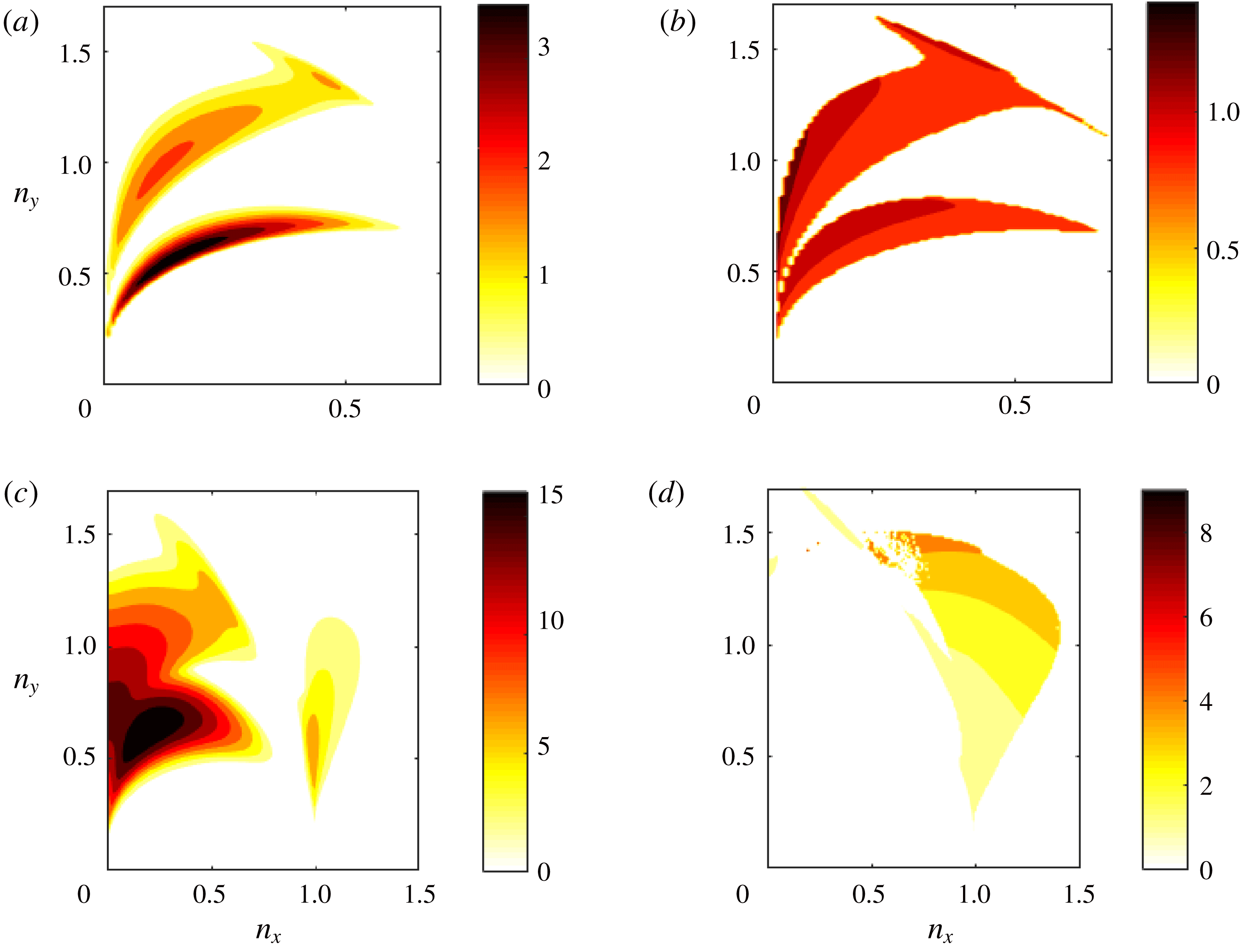
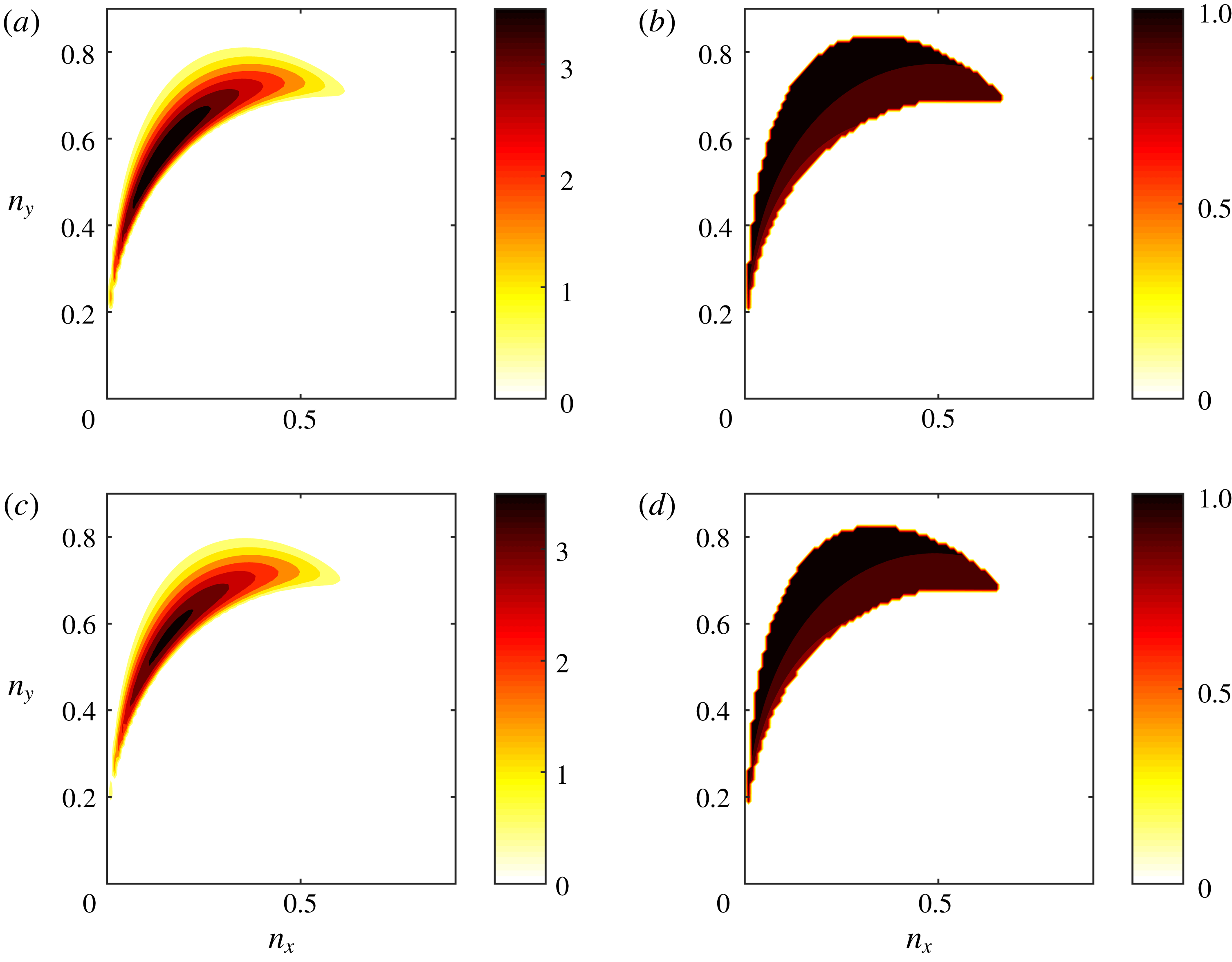
) in the NL simulations is due to the stability of the homogeneous equilibrium to baroclinic perturbations. The growth rate and frequency of the unstable barotropic modes as a function of the mean-flow wavenumber
 $\boldsymbol{n}$
are shown in figure 8 for two values of
 $\unicode[STIX]{x1D700}$
(
 $\unicode[STIX]{x1D700}=10\unicode[STIX]{x1D700}_{c}$
and
 $\unicode[STIX]{x1D700}=50\unicode[STIX]{x1D700}_{c}$
) and for
 $\unicode[STIX]{x1D706}=1$
. At low supercriticality (cf. figure 8
a) only non-zonal modes (
 $n_{x}\neq 0$
) are unstable with two branches of instability: one at meridional scales comparable to the forcing scale (
 $n_{y}\simeq 1$
) and one at larger meridional scales, with the most unstable modes having larger scales than that of the excitation. The frequencies of the unstable modes are very close to the frequencies of the free barotropic Rossby waves
 $\unicode[STIX]{x1D70E}_{Rt}=\unicode[STIX]{x1D6FD}n_{x}/n^{2}$
. This can be quantified by values of one for the ratio
 $R_{ft}=\unicode[STIX]{x1D70E}_{i}/\unicode[STIX]{x1D70E}_{Rt}$
, which is plotted in figure 8(b). At larger supercriticality (cf. figure 8
c) the two branches merge, stationary (
 $\unicode[STIX]{x1D70E}_{i}=0$
) barotropic zonal jet eigenfunctions (
 $n_{x}=0$
) become unstable and there is an additional branch of unstable non-zonal modes with zonal wavenumbers comparable to the excitation wavenumber (
 $n_{x}\simeq 1$
) with the frequency of these modes departing substantially from the Rossby wave frequency (cf. figure 8
d). However, the large-scale non-zonal structures, remain the most unstable modes.
Dispersion properties of the unstable barotropic modes for
 $\unicode[STIX]{x1D6FD}=100$
,
 $\unicode[STIX]{x1D706}=1$
. (a,c) Growth rate
 $\unicode[STIX]{x1D70E}_{r}$
of the most unstable modes for (a)
 $\unicode[STIX]{x1D700}=10\unicode[STIX]{x1D700}_{c}$
and (c)
 $\unicode[STIX]{x1D700}=100\unicode[STIX]{x1D700}_{c}$
. (b,d) Ratio of the frequency of the most unstable modes over the barotropic Rossby wave frequency
 $R_{ft}=\unicode[STIX]{x1D70E}_{i}/\unicode[STIX]{x1D70E}_{Rt}$
for (b)
 $\unicode[STIX]{x1D700}=10\unicode[STIX]{x1D700}_{c}$
and (d)
 $\unicode[STIX]{x1D700}=100\unicode[STIX]{x1D700}_{c}$
. The forcing in the two layers is uncorrelated (
 $p=0$
).

When
 $\unicode[STIX]{x1D706}<0.68$
, baroclinic modes become S3T unstable and have for small values of
 $\unicode[STIX]{x1D706}$
comparable growth rate to the barotropic modes (or nearly equal in the case
 $\unicode[STIX]{x1D706}\ll 1$
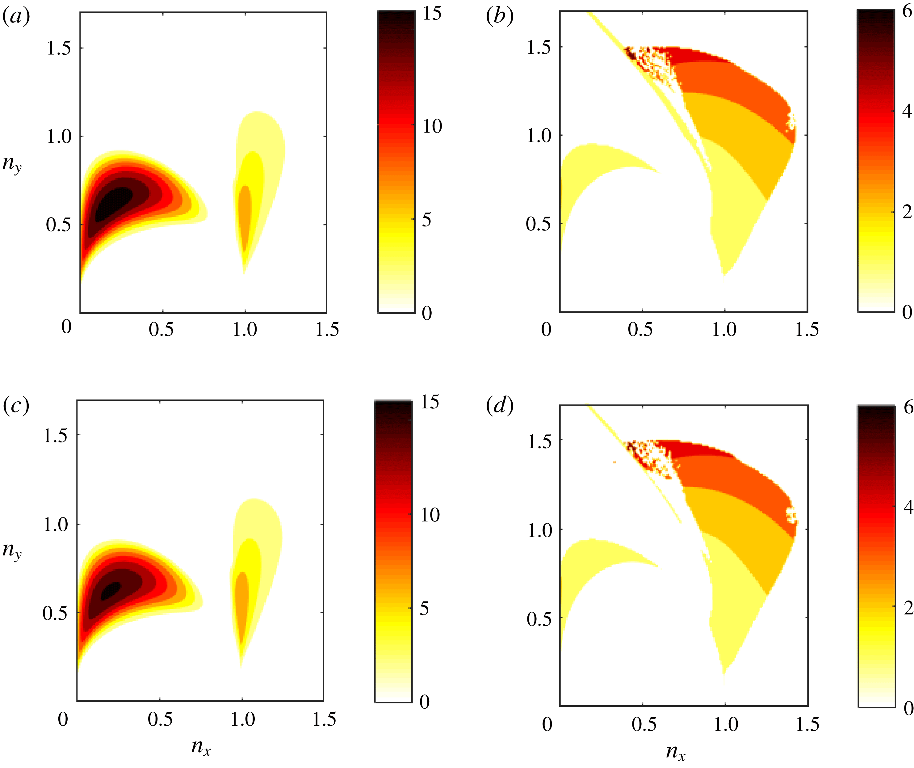
). The growth rate and frequency of the most unstable barotropic and baroclinic modes are shown in figures 9 and 10 for
 $\unicode[STIX]{x1D706}=0.1$
and two values of the energy input rate. The barotropic and baroclinic modes have similar growth rates as a function of
 $\boldsymbol{n}$
. Their dispersion properties resemble the large-scale branch of the unstable barotropic modes at larger values of
 $\unicode[STIX]{x1D706}$
, with the frequencies of the large-scale modes following the dispersion of the barotropic
 $\unicode[STIX]{x1D70E}_{Rt}$
, and baroclinic
 $\unicode[STIX]{x1D70E}_{Rc}=\unicode[STIX]{x1D6FD}n_{x}/n_{\unicode[STIX]{x1D706}}^{2}$
Rossby waves as shown in figure 9(c,d). At larger supercriticalities, stationary barotropic and baroclinic zonal jet eigenfunctions are unstable but the non-zonal modes have larger growth rates (cf. figure 10).
Dispersion properties of the unstable modes for
 $\unicode[STIX]{x1D6FD}=100$
,
 $\unicode[STIX]{x1D706}=0.1$
and
 $\unicode[STIX]{x1D700}=10\unicode[STIX]{x1D700}_{c}$
. (a,c) Growth rate
 $\unicode[STIX]{x1D70E}_{r}$
of the most unstable (a) barotropic and (c) baroclinic modes. (b,d) Ratio of the frequency of the most unstable (b) barotropic modes over the corresponding barotropic Rossby wave frequency
 $R_{ft}=\unicode[STIX]{x1D70E}_{i}/\unicode[STIX]{x1D70E}_{Rt}$
and (d) baroclinic modes over the corresponding baroclinic Rossby wave frequency
 $R_{fc}=\unicode[STIX]{x1D70E}_{i}/\unicode[STIX]{x1D70E}_{Rc}$
. The forcing is uncorrelated (
 $p=0$
).

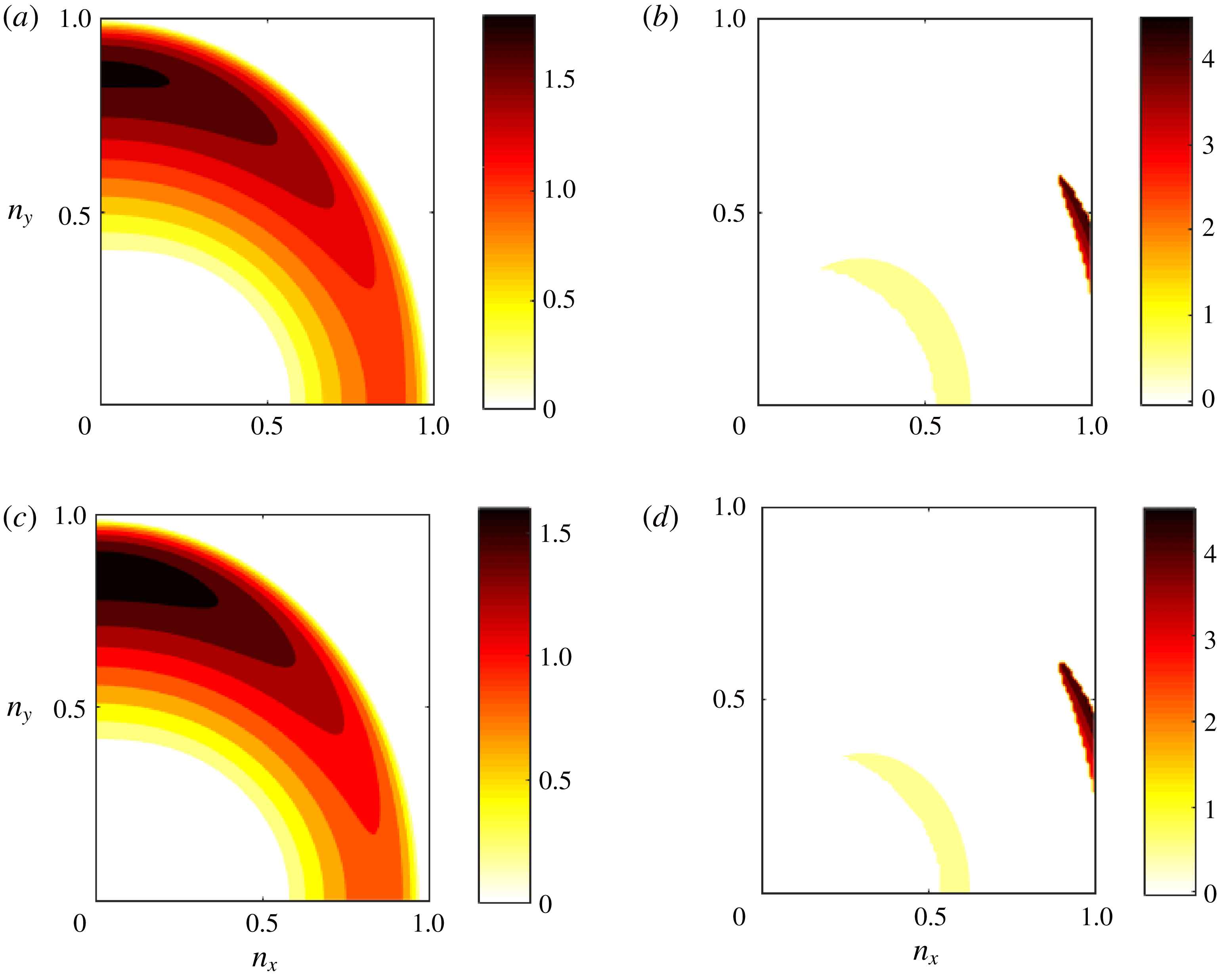
We now consider
 $\unicode[STIX]{x1D6FD}=1$
. Baroclinic modes are unstable for
 $\unicode[STIX]{x1D706}<0.37$
instead of
 $\unicode[STIX]{x1D706}<0.68$
at
 $\unicode[STIX]{x1D6FD}=100$
and the baroclinic unstable modes have lower growth rates than the barotropic modes. This is illustrated in figure 11 where the growth rate and frequency of the unstable barotropic and baroclinic modes are shown for
 $\unicode[STIX]{x1D706}=0.1$
. As in a one-layer fluid, the most unstable modes are stationary zonal jets for
 $\unicode[STIX]{x1D6FD}=\mathit{O}(1)$
. For
 $\unicode[STIX]{x1D706}>0.37$
the dispersion properties of the barotropic unstable modes are similar and are not shown.
We finally test the sensitivity of the dispersion properties of the unstable modes to the forcing correlation between the two layers. Consider first the barotropic forcing (
 $p=1$
). In this case the flux feedbacks arise only from the first terms in (4.5)–(4.6), that is only from the organization of the barotropic turbulent eddies by the mean flow. For
 $\unicode[STIX]{x1D706}=\mathit{O}(1)$
the baroclinic modes are stable and the dispersion properties of the barotropic modes are similar to the ones shown in figure 8 with the only significant difference being the absence of the upper branch. For lower values of
 $\unicode[STIX]{x1D706}$
, the baroclinic modes become unstable and have dispersion properties similar to the ones shown in figures 9 and 10 for uncorrelated forcing despite the fact that small-scale incoherent baroclinic eddies are not directly excited in this case (
 $S_{E}^{\unicode[STIX]{x1D703}\unicode[STIX]{x1D703}}=0$
). Therefore the instability of the baroclinic modes when excitation occurs at much smaller scales than the Rossby radius of deformation is robust regardless of whether incoherent baroclinic eddies are supported at the homogeneous equilibrium.
The same as figure 9 but for
 $\unicode[STIX]{x1D700}=100\unicode[STIX]{x1D700}_{c}$
.

We then consider the baroclinic forcing (
 $p=-1$
), in which case the flux feedbacks arise only from the organization of the baroclinic turbulent eddies by the mean flow (i.e. the second terms in (4.5)–(4.6)). For low values of
 $\unicode[STIX]{x1D706}$
, the dispersion properties of both the barotropic and the baroclinic modes are similar to the ones obtained for uncorrelated forcing (
 $p=0$
) (shown in figure 9) and are not shown. The dispersion properties at
 $\unicode[STIX]{x1D706}=1$
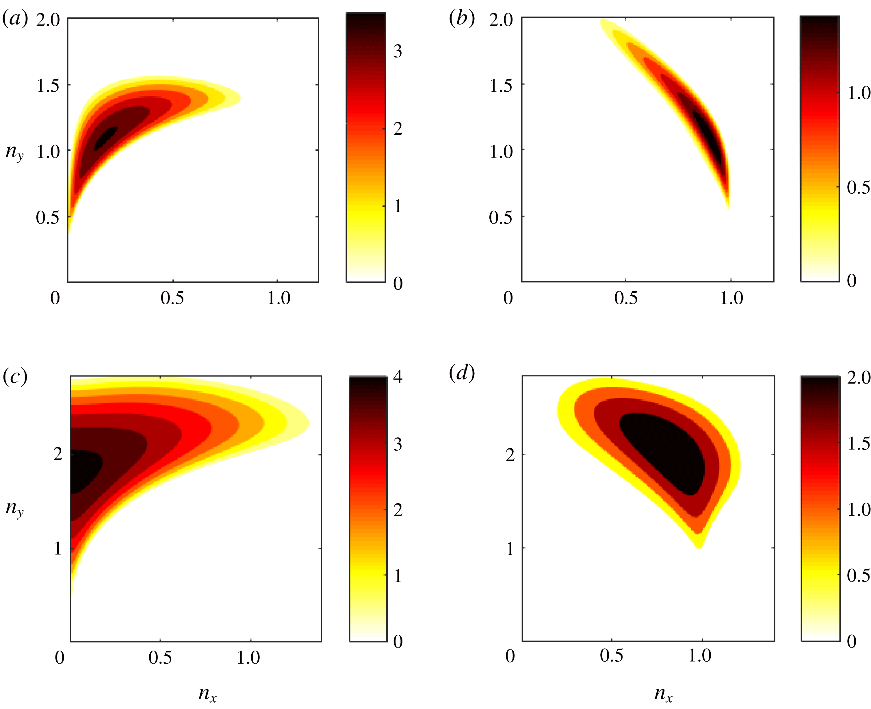
are shown in figure 12(a,b). We observe that barotropic modes have faster growth rates and resemble the upper branch of figure 8, that is they have small zonal scales and meridional scales comparable to the forcing scale (
 $n_{y}\simeq 1$
). The most unstable baroclinic modes, that are suboptimal compared to their barotropic counterparts, have both zonal and meridional scales comparable to the forcing scale. Interestingly, when we force at scales larger than the Rossby radius of deformation (
 $\unicode[STIX]{x1D706}>1$
), the instability characteristics change. As illustrated in figure 12(c,d) showing the dispersion properties at
 $\unicode[STIX]{x1D706}=2$
, the most unstable modes are barotropic zonal jets with scales comparable to the deformation scale, a characteristic that is also evident at even larger values of
 $\unicode[STIX]{x1D706}$
.
In summary, S3T predicts that the homogeneous statistical equilibrium of a two-layer baroclinic flow becomes unstable at a critical value of the energy input rate,
 $\unicode[STIX]{x1D700}_{c}$
, whereupon large-scale mean flows emerge. Barotropic modes have larger growth rates compared to their baroclinic counterparts for all values of
 $\unicode[STIX]{x1D6FD}$
and
 $\unicode[STIX]{x1D706}$
regardless of the characteristics of the eddies supported at statistical equilibrium. When energy is injected at a length scale close to the deformation radius, barotropic modes following the Rossby wave dispersion have in general the largest growth rate for large values of
 $\unicode[STIX]{x1D6FD}$
and stationary zonal jets have the largest growth rate for
 $\unicode[STIX]{x1D6FD}=\mathit{O}(1)$
. When energy is injected at scales much smaller than the deformation radius, both barotropic and baroclinic large-scale flows emerge with the barotropic modes having slightly larger growth rates.
Dispersion properties of the unstable modes for
 $\unicode[STIX]{x1D6FD}=1$
,
 $\unicode[STIX]{x1D706}=0.1$
and
 $\unicode[STIX]{x1D700}=10\unicode[STIX]{x1D700}_{c}$
. (a,c) Growth rate
 $\unicode[STIX]{x1D70E}_{r}$
of the most unstable (a) barotropic and (c) baroclinic modes. (b,d) Frequency
 $\unicode[STIX]{x1D70E}_{i}$
of the most unstable (b) barotropic and (d) baroclinic modes.

Dispersion properties of the unstable modes for baroclinic forcing (
 $p=-1$
) at
 $\unicode[STIX]{x1D6FD}=100$
and
 $\unicode[STIX]{x1D700}=10\unicode[STIX]{x1D700}_{c}$
. (a,b) Growth rate
 $\unicode[STIX]{x1D70E}_{r}$
of the most unstable (a) barotropic and (b) baroclinic modes for
 $\unicode[STIX]{x1D706}=1$
. (c,d) Growth rate
 $\unicode[STIX]{x1D70E}_{r}$
of the most unstable (c) barotropic and (d) baroclinic modes when
 $\unicode[STIX]{x1D706}=2$
.

5 Equilibration of the SSD instabilities and comparison to NL simulations
In this section we examine the equilibration of the SSD instabilities by numerical integrations of the S3T dynamical system. The goal is twofold. The first is to determine the non-homogeneous fixed points of the S3T dynamical system with the largest domain of attraction that a random perturbation will likely end up at. For example, we saw in the previous section that when the non-dimensional radius of deformation is smaller than a critical value, barotropic and baroclinic modes have comparable growth rates. Therefore there is the question of whether the equilibrated state will consist of both barotropic and baroclinic components. The second is to compare the dominant structures in the turbulent flow with the equilibrated states in the S3T system and to investigate whether the characteristics of the dominant structures in the NL simulations are predicted by S3T.
To integrate the S3T dynamical system, we discretize (3.12)–(3.14) in a doubly periodic channel of size
 $2\unicode[STIX]{x03C0}\times 2\unicode[STIX]{x03C0}$
using a pseudo-spectral code and a fourth-order time stepping Runge–Kutta scheme. Due to the high-dimensionality of the covariance matrix we use the modest
 $M=32\times 32$
resolution. To facilitate the comparison with the NL simulations, we apply the same ring forcing (3.1) and consider the same parameters
 $\tilde{\unicode[STIX]{x1D6FD}}=60$
,
 $\tilde{r}=0.1$
,
 $\tilde{k}_{f}=6$
and
 $\unicode[STIX]{x0394}\tilde{k}_{f}=1$
. Because the S3T simulations are computationally expensive, we also utilize for comparison purposes simulations of the ensemble quasi-linear system (EQL) defined in (3.2), (3.3) and (3.6). The EQL system is the finite ensemble version of the deterministic S3T dynamical system and the EQL simulations converge to the S3T integrations as the number of ensemble members
 $N_{ens}$
used to calculate the mean increases. The emergent structures and the statistical turbulent equilibria predicted by the S3T system manifest in the EQL integrations with the addition of noise from stochastic forcing fluctuations, which for any finite
 $N_{ens}$
do not average to zero. A disadvantage of this method is that due to thermal noise from the excitation, only the equilibria with the largest domain of attraction will emerge. Previous studies have investigated the convergence of the EQL simulations to the S3T integrations and determined that
 $N_{ens}=10$
ensemble members illustrate the relevant dynamics with minimal computational cost (Bakas & Ioannou Reference Bakas and Ioannou2014). We therefore make the same choice.
Consider first the case of uncorrelated forcing between the layers (
 $p=0$
) and
 $\tilde{\unicode[STIX]{x1D706}}=\tilde{k}_{f}$
. The critical energy input rate
 $\tilde{\unicode[STIX]{x1D700}}_{c}$
that renders the homogeneous S3T equilibrium unstable is obtained from the discrete version of (4.3)–(4.4). We investigate the equilibration of the SSD instability for supercritical values of
 $\tilde{\unicode[STIX]{x1D700}}$
through S3T integrations. For
 $\tilde{\unicode[STIX]{x1D700}}=2\tilde{\unicode[STIX]{x1D700}}_{c}$
, the barotropic perturbation with
 $({\tilde{n}}_{x},{\tilde{n}}_{y})=(1,4)$
has the largest growth rate, while the baroclinic perturbations are S3T stable at this value of
 $\tilde{\unicode[STIX]{x1D706}}$
for all values of
 $\tilde{\unicode[STIX]{x1D700}}$
. At
 $t=0$
, we introduce a small random perturbation, with both barotropic and baroclinic mean-flow components. The baroclinic part of the flow diminishes while the barotropic part of the flow grows exponentially with the predicted growth rate, and the flow finally equilibrates to a westward propagating wave. The barotropic streamfunction at equilibrium, shown in figure 13(a), has Fourier components primarily with wavenumbers
 $(|\tilde{k}_{x}|,|\tilde{k}_{y}|)=(1,4)$
and secondarily with wavenumbers
 $(|\tilde{k}_{x}|,|\tilde{k}_{y}|)=(2,4)$
. Investigation of the propagation properties of the wave shows that the phase speed of each wave component is very close to the phase speed of the unstable modes that themselves are nearly equal to the Rossby wave phase speed for each component. The finite amplitude state of the SSD consisting of the propagating waves becomes itself secondarily unstable at larger energy input rates to zonal jet perturbations. This secondary SSD instability has already been discussed in the context of a single layer barotropic flow on a
 $\unicode[STIX]{x1D6FD}$
-plane by Bakas & Ioannou (Reference Bakas and Ioannou2014) and for the chosen parameters it occurs at
 $\tilde{\unicode[STIX]{x1D700}}_{nl}=15\tilde{\unicode[STIX]{x1D700}}_{c}$
. The flow then transitions to a new equilibrium state such as the one shown in figure 13(b) for the case
 $\tilde{\unicode[STIX]{x1D700}}=60\tilde{\unicode[STIX]{x1D700}}_{c}$
. This state consists of a zonal jet with an embedded propagating wave of lower amplitude, as in single-layer barotropic flows (Bakas & Ioannou Reference Bakas and Ioannou2014; Constantinou et al.
Reference Constantinou, Farrell and Ioannou2016).
Contours of mean-flow barotropic streamfunction
 $\unicode[STIX]{x1D6F9}$
at equilibrium for (a)
 $\tilde{\unicode[STIX]{x1D700}}=2\tilde{\unicode[STIX]{x1D700}}_{c}$
and (b)
 $\tilde{\unicode[STIX]{x1D700}}=60\tilde{\unicode[STIX]{x1D700}}_{c}$
. The parameters values are the same as in figure 1.

(a) Kinetic energy power spectrum of the barotropic part of the eddy covariance
 $k^{2}{\hat{S}}^{\unicode[STIX]{x1D713}\unicode[STIX]{x1D713}}$
. (b,c) Total kinetic energy power spectrum of the (b) barotropic (
 $\hat{E}_{S3T}^{\unicode[STIX]{x1D713}}$
) and (c) baroclinic (
 $\hat{E}_{S3T}^{\unicode[STIX]{x1D703}}$
) part of the flow for
 $\tilde{\unicode[STIX]{x1D700}}=2\tilde{\unicode[STIX]{x1D700}}_{c}$
. (d–f) The same as in (a–c) but for
 $\tilde{\unicode[STIX]{x1D700}}=60\tilde{\unicode[STIX]{x1D700}}_{c}$
.

We now investigate how these results relate to the regime transitions and to the characteristics of the dominant structures in the turbulent flow. The rapid increase of the nzmf index in the NL simulations when the energy input rate passes the critical value
 $\tilde{\unicode[STIX]{x1D700}}_{c}$
calculated from the stability analysis of the homogeneous fixed point of the SSD shows that the bifurcation point for the emergence of large-scale waves in the turbulent flow is accurately predicted by S3T. The same holds for the increase of the zmf index observed in figure 1 for
 $\tilde{\unicode[STIX]{x1D700}}\gtrapprox 12\tilde{\unicode[STIX]{x1D700}}_{c}$
, which shows that zonal jets emerge in the flow approximately at the stability threshold
 $\tilde{\unicode[STIX]{x1D700}}_{nl}$
of the finite amplitude travelling wave states. The small quantitative discrepancy observed should be attributed to both the thermal noise in the NL simulations and in the quasi-linear approximation of the dynamics. The scales and phase speeds of the dominant large-scale structures in the NL simulations also match the scales and phase speeds of the equilibrated SSD instabilities in S3T. This is illustrated by comparing the distinct peaks in the kinetic energy power spectra in the NL simulations and the frequency power spectrum of the wave components shown in figures 3 and 4 to the scales of the emergent structures in the S3T simulations shown in figure 13 and their phase speed. In order to compare the amplitude of the emergent structures we calculate the equivalent kinetic energy power spectra
 $$\begin{eqnarray}\hat{E}_{S3T}^{\unicode[STIX]{x1D713}}(\tilde{\boldsymbol{k}})=\tilde{k}^{2}(|\hat{\unicode[STIX]{x1D6F9}}|^{2}+{\hat{S}}^{\unicode[STIX]{x1D713}\unicode[STIX]{x1D713}}),\quad \hat{E}_{S3T}^{\unicode[STIX]{x1D703}}(\tilde{\boldsymbol{k}})=\tilde{k}^{2}(|\hat{\unicode[STIX]{x1D6E9}}|^{2}+{\hat{S}}^{\unicode[STIX]{x1D703}\unicode[STIX]{x1D703}}),\end{eqnarray}$$
where
 ${\hat{S}}^{\unicode[STIX]{x1D713}\unicode[STIX]{x1D713}}$
and
 ${\hat{S}}^{\unicode[STIX]{x1D703}\unicode[STIX]{x1D703}}$
are the power spectra of the eddy covariances
 $S^{\unicode[STIX]{x1D713}\unicode[STIX]{x1D713}}$
and
 $S^{\unicode[STIX]{x1D703}\unicode[STIX]{x1D703}}$
respectively. For the barotropic part, the eddy power spectrum
 ${\hat{S}}^{\unicode[STIX]{x1D713}\unicode[STIX]{x1D713}}$
shown in figure 14(a,d) is two orders of magnitude smaller than
 $|\hat{\unicode[STIX]{x1D6F9}}|^{2}$
, so the equivalent power spectrum
 $\hat{E}_{S3T}^{\unicode[STIX]{x1D713}}$
shown in figure 14(b,e) is dominated by the spectrum of the coherent part of the flow. This should come as no surprise, since the dominant structures in the turbulent flow are phase coherent and should therefore be a manifestation of the coherent part of the flow. For the baroclinic part,
 $\unicode[STIX]{x1D6E9}=0$
, so
 $\hat{E}_{S3T}^{\unicode[STIX]{x1D703}}$
that is shown in figure 14(c,e) coincides with the eddy power spectrum
 ${\hat{S}}^{\unicode[STIX]{x1D703}\unicode[STIX]{x1D703}}$
. Comparison of the spectra obtained from the NL simulations (figures 3 and 4) and the equivalent spectrum shown in figure 14 shows that the amplitude of the emergent structures differs by a factor of two for
 $\tilde{\unicode[STIX]{x1D700}}=2\tilde{\unicode[STIX]{x1D700}}_{c}$
and by approximately 20 % for
 $\tilde{\unicode[STIX]{x1D700}}=60\tilde{\unicode[STIX]{x1D700}}_{c}$
. To facilitate comparison of the amplitude of the emerging structures for a wide range of values for
 $\tilde{\unicode[STIX]{x1D700}}$
, we utilize the EQL simulations and calculate the zmf and nzmf indices that are shown in figure 1. We observe that, apart from the quantitative disagreement at low supercritical energy input rates for the amplitude of the emergent waves, the EQL dynamics fairly reproduces the amplitude of the emergent structures. Similar results regarding the comparison of the S3T predictions with NL simulations were found for barotropic turbulence (Bakas & Ioannou Reference Bakas and Ioannou2014), showing that the quasi-linear dynamics close to the bifurcation point captures the emergence of flows in contrast to the physical intuition on the importance of the nonlinear terms as also discussed in the introduction.
Consider now
 $\tilde{\unicode[STIX]{x1D706}}=\tilde{k}_{f}/6$
(
 $\unicode[STIX]{x1D706}=1/6$
) for which the S3T stability analysis predicts the existence of both barotropic and baroclinic unstable S3T modes. We have identified in this case three attracting equilibrium states with finite amplitude mean flows. The first is a purely barotropic equilibrium, to which all purely barotropic perturbations are attracted. Note that purely barotropic perturbations do not produce any baroclinic fluxes even in their nonlinear stage of evolution and as a result, the mean flow remains barotropic. An example of such an equilibrated state is shown for
 $\tilde{\unicode[STIX]{x1D700}}=10\tilde{\unicode[STIX]{x1D700}}_{c}$
in figure 15(a), where again the large-scale flow is a westward propagating wave. However this equilibrium is secondarily unstable to baroclinic mean-flow perturbations. We illustrate this by perturbing the barotropic equilibrium, shown in figure 15(a), with a small baroclinic mean flow perturbation. Figure 15(b) shows the evolution of the baroclinicity measure (2.15) in which
 $\hat{\unicode[STIX]{x1D713}}=\hat{\unicode[STIX]{x1D6F9}}$
and
 $\hat{\unicode[STIX]{x1D703}}=\hat{\unicode[STIX]{x1D6E9}}$
are the Fourier components of the barotropic and baroclinic mean-flow streamfunction respectively. We observe that the baroclinic mean-flow component grows exponentially at first and as soon as it reaches a finite amplitude, the flow transitions to the second non-zonal equilibrium with both barotropic and baroclinic components and baroclinicity
 $R_{b}\simeq 1/4$
. The structure of these components is shown in figure 15(c,d).
(a) Contours of mean-flow barotropic streamfunction
 $\unicode[STIX]{x1D6F9}$
for the pure barotropic equilibrated state. (b) Evolution of the baroclinicity ratio after inserting a baroclinic mean-flow perturbation to the barotropic equilibrium shown in (a). (c,d) Contours of mean flow (c) barotropic
 $\unicode[STIX]{x1D6F9}$
and (d) baroclinic
 $\unicode[STIX]{x1D6E9}$
streamfunction for the mixed barotropic–baroclinic equilibrium state.
 $\tilde{\unicode[STIX]{x1D700}}=10\tilde{\unicode[STIX]{x1D700}}_{c}$
,
 $\tilde{\unicode[STIX]{x1D706}}=\tilde{k}_{f}/6$
and the rest of the parameters are as in figure 13.

The third equilibrium is also a westward propagating wave with both barotropic and baroclinic components and similar scale as the one shown in figure 15(c,d) but is more baroclinic (
 $R_{b}\simeq 2$
). However, this equilibrium has a very small domain of attraction and it can be approached only if the initial perturbation is baroclinic. (Specifically, this equilibrium is approached only if the initial perturbation has a baroclinicity ratio larger than
 $10^{6}$
.) As a result, we do not expect this equilibrium to manifest in noisy simulations of the turbulent flow in which both baroclinic and barotropic perturbations inevitably arise. Therefore, at low supercriticalities the S3T instabilities equilibrate to the finite amplitude mixed barotropic–baroclinic travelling wave shown in figure 15(c,d) with baroclinic to barotropic streamfunction amplitude ratio of approximately one half.
Evolution of the energy of the zonal part of the flow when a zonal mean-flow perturbation is imposed on the finite amplitude equilibrium state shown in the upper insets. The lower insets show the barotropic and baroclinic streamfunction of the mean flow at
 $\tilde{t}=130$
. The energy input rate is
 $\tilde{\unicode[STIX]{x1D700}}=40\tilde{\unicode[STIX]{x1D700}}_{c}$
, and the rest of the parameters are as in figure 15.

Again, at higher supercriticality the traveling baroclinic wave states of the SSD become secondarily unstable to zonal perturbations. However, only the barotropic part of the flow is zonated. This is shown in the numerical integration for
 $\tilde{\unicode[STIX]{x1D700}}=40\tilde{\unicode[STIX]{x1D700}}_{c}$
illustrated in figure 16. In this experiment the mixed barotropic–baroclinic traveling wave state, shown in the upper inset of figure 16, is perturbed by a zonal mean flow perturbation with both barotropic and baroclinic components. The energy of the zonal part of the flow,
 $\tilde{E}_{z}$
, grows exponentially and the flow transitions to the state shown at the lower inset that consists of a zonal barotropic flow and a travelling baroclinic wave. This is a time-dependent state as shown in figure 17. The energy of the zonal part of the flow and the baroclinicity
 $R_{b}$
oscillate and are anti-correlated, revealing that the large-scale flow vacillates between the state shown in figure 18(a,b) where the barotropic zonal jet is dominant and the state shown in figure 18(c,d) where the baroclinic wave is dominant. At even higher energy input rates the large-scale flow exhibits the same time dependence but with weaker fluctuations due to the weakening of the baroclinic wave component.
(a) Evolution of the mean-flow energy (dotted), the energy of the zonal part (solid) and the energy of the non-zonal part (dashed) of the flow. (b) Evolution of the baroclinicity
 $R_{b}$
. The vertical lines denote the times at which the snapshots shown in figure 18 are taken.

(a,b) Snapshot of the mean flow (a) barotropic
 $\unicode[STIX]{x1D6F9}$
and (b) baroclinic
 $\unicode[STIX]{x1D6E9}$
streamfunction at
 $\tilde{t}=270$
. (c,d) The same as in (a,b) but for a snapshot at
 $\tilde{t}=325$
.

Comparison of the dominant structures in the NL simulations (cf. figures 5 and 6) to the equilibrated states in S3T with the largest domain of attraction (cf. figures 15–18) demonstrates that the scales of the phase coherent large-scale waves in the turbulent flow are predicted by S3T. Figure 19 shows the equivalent spectra which are dominated in this case as well by the coherent part of the flow. Comparison to the spectra obtained from the NL simulations (cf. figure 5) shows quantitative differences of the order of 20 % for the amplitude of the emergent structures. Differences on the exact points of transition from the wave attractor to the jet attractor are found in this case as well. But even nuances of the dynamics, such as the long-time variability of the turbulent flow at
 $\tilde{\unicode[STIX]{x1D700}}=40\tilde{\unicode[STIX]{x1D700}}_{c}$
with a vacillation between a state with stronger barotropic jet/weaker baroclinic wave and a state with a stronger baroclinic wave/weaker barotropic jet, are captured in S3T with approximately the same time scale as revealed by comparison of figures 6 and 17.
(a) Kinetic energy power spectrum of the barotropic part of the eddy covariance
 $k^{2}{\hat{S}}^{\unicode[STIX]{x1D713}\unicode[STIX]{x1D713}}$
. (b) Equivalent kinetic energy power spectrum
 $\hat{E}_{S3T}^{\unicode[STIX]{x1D713}}$
of the barotropic part of the flow. (c) Kinetic energy power spectrum of the baroclinic part of the eddy covariance
 $k^{2}{\hat{S}}^{\unicode[STIX]{x1D703}\unicode[STIX]{x1D703}}$
and (d) equivalent kinetic energy power spectrum
 $\hat{E}_{S3T}^{\unicode[STIX]{x1D703}}$
of the baroclinic part of the flow for
 $\tilde{\unicode[STIX]{x1D700}}=10\tilde{\unicode[STIX]{x1D700}}_{c}$
.

We now consider the equilibration of the S3T instabilities for the other two cases of forcing correlation, that is exciting only the barotropic (
 $p=1$
) and the baroclinic (
 $p=-1$
) eddies. For the case of barotropic forcing, the instability characteristics as well as their equilibration are similar to the case of uncorrelated forcing between the two layers and are not shown. For the case of baroclinic forcing, structures with small meridional scales are predicted to initially emerge and the low resolution of the S3T calculations is not adequate to resolve these scales. For this reason we choose to study the equilibration of the instabilities with ensemble quasi-linear simulations (EQL) governed by (3.2)–(3.3) and (3.6) at higher resolution (
 $64\times 64$
). Consider first
 $\tilde{\unicode[STIX]{x1D706}}=\tilde{k}_{f}$
(
 $\unicode[STIX]{x1D706}=1$
). At low supercriticality (
 $\tilde{\unicode[STIX]{x1D700}}<5\tilde{\unicode[STIX]{x1D700}}_{c}$
), the baroclinic modes are stable and barotropic Rossby waves that have the largest growth rate equilibrate at finite amplitude as in the case of uncorrelated forcing. The only difference in this case is that these waves have meridional scales comparable to the forcing scale (the most unstable mode has
 $(|{\tilde{n}}_{x}|,|{\tilde{n}}_{y}|)=(1,6)$
). As a result the flow equilibrates to this barotropic travelling wave state. For higher supercriticality (
 $\tilde{\unicode[STIX]{x1D700}}>5\tilde{\unicode[STIX]{x1D700}}_{c}$
), baroclinic modes are rendered unstable as well. However, the finite amplitude equilibria have very weak baroclinicity with the baroclinic streamfunction being one order of magnitude smaller than the barotropic part of the flow that has been zonated through the secondary SSD instability.
Consider now the larger value
 $\tilde{\unicode[STIX]{x1D706}}=2\tilde{k}_{f}$
(
 $\unicode[STIX]{x1D706}=2$
) for which linear stability analysis predicts that barotropic stationary zonal jets with scales close to the Rossby radius of deformation have the largest growth rate. The equilibrated structure for
 $\tilde{\unicode[STIX]{x1D700}}=10\tilde{\unicode[STIX]{x1D700}}_{c}$
that is shown in figure 20(a) indeed consists of a small-scale barotropic jet with a scale comparable to the deformation radius (
 ${\tilde{n}}_{y}=3\tilde{\unicode[STIX]{x1D706}}/4$
). At larger supercriticality, the equilibrated jets assume larger scales (figure 20
b). For all energy input rates the baroclinic streamfunction is orders of magnitude smaller and is therefore not shown. Finally we note that at
 $\tilde{\unicode[STIX]{x1D706}}=\tilde{k}_{f}/6$
the equilibrated structures are similar to the case of uncorrelated forcing and are not shown.
Contours of the barotropic
 $\unicode[STIX]{x1D6F9}$
streamfunction of the equilibrated state for a baroclinic forcing (
 $p=-1$
) and
 $\tilde{\unicode[STIX]{x1D706}}=2\tilde{k}_{f}$
at (a)
 $\tilde{\unicode[STIX]{x1D700}}=10\tilde{\unicode[STIX]{x1D700}}_{c}$
and (b)
 $\tilde{\unicode[STIX]{x1D700}}=60\tilde{\unicode[STIX]{x1D700}}_{c}$
. The flows are obtained from EQL integrations at a
 $64\times 64$
resolution and
 $N_{ens}=10$
ensemble members.

Comparison of the coherent structures in figure 20 with the emergent structures in the NL simulations in figure 7 reveals that again the scales of the emergent flows are accurately captured by S3T, while their amplitude is slightly underestimated.
6 Conclusions
The emergence of coherent structures in stratified turbulent flows with turbulence supported by external sources was investigated in this work. A two-layer model on a
 $\unicode[STIX]{x1D6FD}$
-plane channel was considered under the influence of homogeneous and isotropic stochastic forcing and linear damping of potential vorticity. No mean thermal gradient was imposed in the flow. The goal was to extend the analysis of studies in barotropic turbulence which found that (i) coherent flows emerge out of a background of homogeneous turbulence as a bifurcation when the turbulence intensity increases and (ii) these turbulent bifurcations can be attributed to a new type of collective instability of the statistical state dynamics of the turbulent flow. The question addressed was the following: in the absence of temperature gradients can externally forced turbulence in a stratified flow support turbulent equilibria in which large-scale baroclinic coherent flows are sustained at finite amplitude? Or are the large-scale flows that emerge barotropic?
Direct nonlinear simulations show two major flow transitions as the energy input rate of the forcing increases. In the first transition large-scale Rossby waves that remain phase coherent over long time scales emerge in the flow. As the energy input rate increases, the scales of these waves and their energy increases as well. In the second transition, zonal jets emerge instead while the energy in the large-scale waves decreases. Regarding the vertical structure of the emergent flows, the large-scale waves and jets are barotropic when energy is injected at scales comparable to the Rossby radius of deformation. When the energy is injected at smaller scales, the waves that emerge have comparable barotropic and baroclinic streamfunctions. After the second transition, the barotropic part of the flow is zonated and the turbulent flow exhibits variability on long times scales with time periods of stronger barotropic jet and time periods of stronger baroclinic waves. For larger energy input rates the barotropic jet dominates. These results were found to be independent of the correlation of the excitation between the two layers as two extreme cases (forcing only baroclinic eddies and forcing only barotropic eddies) produced qualitatively similar results to the case of uncorrelated forcing between the two layers. That is, even though the forcing might inject only barotropic eddies in the flow, these eddies are organized to support coherent baroclinic waves. Similarly, in the case in which we inject only baroclinic eddies in the flow, the prevalence of barotropic coherent structures remains.
We then developed a theory to explain the emergence of coherent flows and predict their characteristics. The theory is based on a second-order closure of the statistical state dynamics (SSD) of the turbulent flow (S3T). The fixed points of the S3T dynamical system for the joint evolution of the coherent flow and the eddy covariance define equilibria, the manifestations of which are the states of the turbulent flow at statistical equilibrium. Instability of these fixed points and equilibration into new steady states manifest as regime transitions in the turbulent flow with the emergence of new attractors. The linear stability of the homogeneous equilibrium with no coherent structures was examined analytically for a wide range of forcing scales
 $1/\tilde{k}_{f}$
relative to the deformation radius
 $1/\tilde{\unicode[STIX]{x1D706}}$
and a wide range of values for the non-dimensional planetary vorticity gradient
 $\unicode[STIX]{x1D6FD}=\tilde{\unicode[STIX]{x1D6FD}}\tilde{r}/\tilde{k}_{f}$
, where
 $1/\tilde{r}$
is the linear dissipation time scale. The equilibrium was found to be unstable for all
 $\tilde{\unicode[STIX]{x1D706}}$
when the energy input rate of the forcing exceeds a critical value.
When turbulence is injected close to the Rossby radius of deformation or at larger scales, baroclinic waves are either stable or grow at a lower rate compared to barotropic waves. For large values of
 $\unicode[STIX]{x1D6FD}$
, westward propagating barotropic waves that follow the barotropic Rossby wave dispersion grow the most, while for values of
 $\unicode[STIX]{x1D6FD}=\mathit{O}(1)$
or lower stationary zonal jets have faster growth rates. The equilibration of the incipient instabilities was then studied for large values of
 $\unicode[STIX]{x1D6FD}$
through numerical integrations of the S3T dynamical system. The flow was found to equilibrate for low supercriticality at finite amplitude travelling wave states that approximately have the same dispersion properties as the unstable modes. For larger supercriticality, the travelling wave states become S3T unstable with respect to zonal jet perturbations. The flow then equilibrates at mixed jet–travelling wave states with lower amplitude travelling waves embedded within strong zonal jets. This dynamics is similar to barotropic turbulence organization that was investigated in earlier studies (Bakas & Ioannou Reference Bakas and Ioannou2014; Constantinou et al.
Reference Constantinou, Farrell and Ioannou2016).
When turbulence is injected at scales much smaller than the deformation radius, barotropic and baroclinic modes have comparable growth rates with barotropic modes growing at slightly faster rates and having dispersion properties similar to the ones for larger values of the deformation radius. For low supercriticalities, the flow equilibrates at mixed barotropic–baroclinic travelling wave states with the barotropic streamfunction having a larger amplitude compared to the baroclinic streamfunction. For higher supercriticalities, a secondary S3T instability of the travelling wave state similar to the one discussed above zonates the barotropic part of the flow. As a result the flow transitions to a mixed barotropic–baroclinic jet–wave state where a weaker baroclinic wave is embedded in a stronger barotropic jet. This state is time dependent with the amplitudes of the barotropic jet and the baroclinic wave oscillating in time as the jet intensifies the wave for half a cycle and the wave intensifies the jet in the next part of the cycle giving the excess energy back to the jet. For highly supercritical regimes, the baroclinicity and this vacillation are much weaker. Finally, it was found that the characteristics of the emergent structures are not sensitive to the correlation of the forcing in the two layers (with small exceptions in the case of baroclinic forcing).
The predictions of the theory were then compared to the results obtained in direct numerical nonlinear simulations. First of all, the absence of baroclinic structures in the turbulent flow when the energy is injected at scales comparable to the deformation radius, is attributed to the stability of the homogeneous equilibrium to baroclinic modes. The critical threshold above which non-zonal structures are unstable according to the stability analysis was found to be in excellent agreement with the critical value above which the large-scale waves acquire significant power in nonlinear simulations. The scale and phase speed of the dominant structures in the nonlinear simulations were also found to correspond to the coherent structures predicted by S3T including the existence or not of a baroclinic component for the flow. However, the amplitude of the emerging waves is underestimated. In addition, the critical turbulence intensity threshold for the emergence of zonal jets, which is identified in S3T as the energy input rate at which the secondary instability of the finite amplitude travelling wave states appears, was also found to roughly match the corresponding threshold for jet formation in the nonlinear simulations. The emerging jet scale is accurately predicted by S3T, while its amplitude is underestimated by approximately 20 %. However, it is surprising that even nuances of the statistical state dynamics such as the time-dependent mixed barotropic–baroclinic jet–wave state have a manifestation in the turbulent flow. We also note that the predictions of the second-order closure of the SSD are accurately reflected in single realizations of the turbulent flow with the large-scale structure emerging as predicted even for parameters close to the bifurcation points, when the flows are relatively weak.
In summary, in stratified flows with no mean thermal gradient imposed, there is a large bias towards the emergence of barotropic flows from the organization of both barotropic and baroclinic turbulent eddies. This tendency for deep barotropic flows was observed in recent work addressing the dynamics of jets in the gaseous planets. Farrell & Ioannou (Reference Farrell and Ioannou2017) used a second-order closure of the SSD for the QG dynamics of a two-layer model with bottom friction and found that, in the limit of small friction, the zonal jets assume a universal barotropic structure. Liu & Schneider (Reference Liu and Schneider2015) used a realistic model of the circulation in the Jovian atmosphere driven by large-scale thermal heating and dissipated by magnetohydrodynamic drag at the bottom of the domain and found the same tendency for barotropic structures in the limit of small drag. This tendency is also observed in very recent observational results of the Juno mission obtained by measurements of the asymmetries in the gravity field of Jupiter, which indicated that the Jovian jets reach a depth of approximately 3000 km (Kaspi et al. Reference Kaspi, Galanti, Hubbard, Stevenson, Bolton, Iess, Guillot, Bloxham, Connerney, Cao, Durante, Folkner, Helled, Ingersoll, Levin, Lunine, Miguel, Militzer, Parisi and Wahl2018).
Acknowledgements
The authors would like to thank N. Constantinou for useful discussions. N.A.B. is supported by the AXA Research Fund.
Appendix A. Stability equation
It can be shown, as in the barotropic case (Bakas & Ioannou Reference Bakas and Ioannou2014), that due to the homogeneity of the forcing covariance, the state with zero coherent flow
 $[Z,H]^{\text{T}}=0$
and a homogeneous covariance
 $\unicode[STIX]{x1D63E}_{E}=\unicode[STIX]{x1D64C}/2$
is a fixed point of the S3T dynamical system. The linear stability of the homogeneous equilibrium is assessed by considering the joint evolution of barotropic and baroclinic mean-flow perturbations
 $[\unicode[STIX]{x1D6FF}\unicode[STIX]{x1D6F9},\unicode[STIX]{x1D6FF}\unicode[STIX]{x1D6E9}]^{\text{T}}$
and covariance perturbations
 $\unicode[STIX]{x1D6FF}\unicode[STIX]{x1D63E}$
. The linearized equations governing the evolution of the mean-flow perturbations are:
 $$\begin{eqnarray}\displaystyle & \unicode[STIX]{x2202}_{t}\unicode[STIX]{x0394}\unicode[STIX]{x1D6FF}\unicode[STIX]{x1D6F9}+\unicode[STIX]{x1D6FD}\unicode[STIX]{x2202}_{x}\unicode[STIX]{x1D6FF}\unicode[STIX]{x1D6F9}=\unicode[STIX]{x1D6FF}f_{\unicode[STIX]{x1D713}}-\unicode[STIX]{x0394}\unicode[STIX]{x1D6FF}\unicode[STIX]{x1D6F9}, & \displaystyle\end{eqnarray}$$
 $$\begin{eqnarray}\displaystyle & \unicode[STIX]{x2202}_{t}\unicode[STIX]{x1D6E5}_{\unicode[STIX]{x1D706}}\unicode[STIX]{x1D6FF}\unicode[STIX]{x1D6E9}+\unicode[STIX]{x1D6FD}\unicode[STIX]{x2202}_{x}\unicode[STIX]{x1D6FF}\unicode[STIX]{x1D6E9}=\unicode[STIX]{x1D6FF}f_{\unicode[STIX]{x1D703}}-\unicode[STIX]{x1D6E5}_{\unicode[STIX]{x1D706}}\unicode[STIX]{x1D6FF}\unicode[STIX]{x1D6E9}, & \displaystyle\end{eqnarray}$$
where
 $\unicode[STIX]{x1D6FF}f_{\unicode[STIX]{x1D713}}=R^{\unicode[STIX]{x1D713}}\left(\unicode[STIX]{x1D6FF}\unicode[STIX]{x1D63E}\right)$
and
 $\unicode[STIX]{x1D6FF}f_{\unicode[STIX]{x1D703}}=R^{\unicode[STIX]{x1D703}}\left(\unicode[STIX]{x1D6FF}\unicode[STIX]{x1D63E}\right)$
are the perturbation eddy stress divergences which depend on the components of
 $\unicode[STIX]{x1D6FF}\unicode[STIX]{x1D63E}$
. The components of
 $\unicode[STIX]{x1D6FF}\unicode[STIX]{x1D63E}$
evolve according to:
 $$\begin{eqnarray}\displaystyle \unicode[STIX]{x2202}_{t}\unicode[STIX]{x1D6FF}C^{\unicode[STIX]{x1D701}\unicode[STIX]{x1D701}} & = & \displaystyle -2\unicode[STIX]{x1D6FF}C^{\unicode[STIX]{x1D701}\unicode[STIX]{x1D701}}-\unicode[STIX]{x1D6FD}\left[\unicode[STIX]{x2202}_{\overline{x}}\left(\tilde{\unicode[STIX]{x1D6E5}}+{\textstyle \frac{1}{4}}\overline{\unicode[STIX]{x1D6E5}}\right)-2\unicode[STIX]{x2202}_{\tilde{x}}\unicode[STIX]{x1D6E4}\right]\unicode[STIX]{x1D6FF}S^{\unicode[STIX]{x1D713}\unicode[STIX]{x1D713}}-(\unicode[STIX]{x1D6FF}\boldsymbol{U}_{a}^{\unicode[STIX]{x1D713}}-\unicode[STIX]{x1D6FF}\boldsymbol{U}_{b}^{\unicode[STIX]{x1D713}})\boldsymbol{\cdot }\tilde{\unicode[STIX]{x1D735}}\tilde{\unicode[STIX]{x1D6E5}}^{2}S_{E}^{\unicode[STIX]{x1D713}\unicode[STIX]{x1D713}}\nonumber\\ \displaystyle & & \displaystyle -\,(\unicode[STIX]{x1D6E5}_{a}\unicode[STIX]{x1D6FF}\boldsymbol{U}_{a}^{\unicode[STIX]{x1D713}}-\unicode[STIX]{x1D6E5}_{b}\unicode[STIX]{x1D6FF}\boldsymbol{U}_{b}^{\unicode[STIX]{x1D713}})\boldsymbol{\cdot }\tilde{\unicode[STIX]{x1D735}}\tilde{\unicode[STIX]{x1D6E5}}S_{E}^{\unicode[STIX]{x1D713}\unicode[STIX]{x1D713}},\end{eqnarray}$$
 $$\begin{eqnarray}\displaystyle \unicode[STIX]{x2202}_{t}\unicode[STIX]{x1D6FF}C^{\unicode[STIX]{x1D701}\unicode[STIX]{x1D702}} & = & \displaystyle \!-[(\unicode[STIX]{x1D6FF}\boldsymbol{U}_{a}^{\unicode[STIX]{x1D703}}\boldsymbol{\cdot }\tilde{\unicode[STIX]{x1D735}})\tilde{\unicode[STIX]{x1D6E5}}\tilde{\unicode[STIX]{x1D6E5}}_{\unicode[STIX]{x1D706}}-(\unicode[STIX]{x1D6E5}_{a}\unicode[STIX]{x1D6FF}\boldsymbol{U}_{a}^{\unicode[STIX]{x1D703}}\boldsymbol{\cdot }\tilde{\unicode[STIX]{x1D735}})\tilde{\unicode[STIX]{x1D6E5}}_{\unicode[STIX]{x1D706}}]S_{E}^{\unicode[STIX]{x1D703}\unicode[STIX]{x1D703}}+[(\unicode[STIX]{x1D6FF}\boldsymbol{U}_{b}^{\unicode[STIX]{x1D703}}\boldsymbol{\cdot }\tilde{\unicode[STIX]{x1D735}})\tilde{\unicode[STIX]{x1D6E5}}^{2}-(\unicode[STIX]{x1D6E5}_{\unicode[STIX]{x1D706},b}\unicode[STIX]{x1D6FF}\boldsymbol{U}_{b}^{\unicode[STIX]{x1D703}}\boldsymbol{\cdot }\tilde{\unicode[STIX]{x1D735}})\tilde{\unicode[STIX]{x1D6E5}}]S_{E}^{\unicode[STIX]{x1D713}\unicode[STIX]{x1D713}}\nonumber\\ \displaystyle & & \displaystyle -\,2\unicode[STIX]{x1D6FF}C^{\unicode[STIX]{x1D701}\unicode[STIX]{x1D702}}-\unicode[STIX]{x1D6FD}\left[{\textstyle \frac{1}{2}}\unicode[STIX]{x2202}_{\overline{x}}\left(\tilde{\unicode[STIX]{x1D6E5}}+\tilde{\unicode[STIX]{x1D6E5}}_{\unicode[STIX]{x1D706}}+{\textstyle \frac{1}{2}}\overline{\unicode[STIX]{x1D6E5}}\right)-\unicode[STIX]{x2202}_{\tilde{x}}(\tilde{\unicode[STIX]{x1D6E5}}-\tilde{\unicode[STIX]{x1D6E5}}_{\unicode[STIX]{x1D706}}+2\unicode[STIX]{x1D6E4})\right]\unicode[STIX]{x1D6FF}S^{\unicode[STIX]{x1D713}\unicode[STIX]{x1D703}},\end{eqnarray}$$
 $$\begin{eqnarray}\displaystyle \unicode[STIX]{x2202}_{t}\unicode[STIX]{x1D6FF}C^{\unicode[STIX]{x1D702}\unicode[STIX]{x1D701}} & = & \displaystyle [(\unicode[STIX]{x1D6FF}\boldsymbol{U}_{b}^{\unicode[STIX]{x1D703}}\boldsymbol{\cdot }\tilde{\unicode[STIX]{x1D735}})\tilde{\unicode[STIX]{x1D6E5}}\tilde{\unicode[STIX]{x1D6E5}}_{\unicode[STIX]{x1D706}}-(\unicode[STIX]{x1D6E5}_{b}\unicode[STIX]{x1D6FF}\boldsymbol{U}_{b}^{\unicode[STIX]{x1D703}}\boldsymbol{\cdot }\tilde{\unicode[STIX]{x1D735}})\tilde{\unicode[STIX]{x1D6E5}}_{\unicode[STIX]{x1D706}}]S_{E}^{\unicode[STIX]{x1D703}\unicode[STIX]{x1D703}}-[(\unicode[STIX]{x1D6FF}\boldsymbol{U}_{a}^{\unicode[STIX]{x1D703}}\boldsymbol{\cdot }\tilde{\unicode[STIX]{x1D735}})\tilde{\unicode[STIX]{x1D6E5}}^{2}-(\unicode[STIX]{x1D6E5}_{\unicode[STIX]{x1D706},a}\unicode[STIX]{x1D6FF}\boldsymbol{U}_{a}^{\unicode[STIX]{x1D703}}\boldsymbol{\cdot }\tilde{\unicode[STIX]{x1D735}})\tilde{\unicode[STIX]{x1D6E5}}]S_{E}^{\unicode[STIX]{x1D713}\unicode[STIX]{x1D713}}\nonumber\\ \displaystyle & & \displaystyle -\,\unicode[STIX]{x1D6FF}C^{\unicode[STIX]{x1D702}\unicode[STIX]{x1D701}}-\unicode[STIX]{x1D6FD}\left[{\textstyle \frac{1}{2}}\unicode[STIX]{x2202}_{\overline{x}}\left(\tilde{\unicode[STIX]{x1D6E5}}+\tilde{\unicode[STIX]{x1D6E5}}_{\unicode[STIX]{x1D706}}+{\textstyle \frac{1}{2}}\overline{\unicode[STIX]{x1D6E5}}\right)-\unicode[STIX]{x2202}_{\tilde{x}}(\tilde{\unicode[STIX]{x1D6E5}}_{\unicode[STIX]{x1D706}}-\tilde{\unicode[STIX]{x1D6E5}}+2\unicode[STIX]{x1D6E4})\right]\unicode[STIX]{x1D6FF}S^{\unicode[STIX]{x1D703}\unicode[STIX]{x1D713}},\end{eqnarray}$$
 $$\begin{eqnarray}\displaystyle \unicode[STIX]{x2202}_{t}\unicode[STIX]{x1D6FF}C^{\unicode[STIX]{x1D702}\unicode[STIX]{x1D702}} & = & \displaystyle -[(\unicode[STIX]{x1D6FF}\boldsymbol{U}_{a}^{\unicode[STIX]{x1D713}}-\unicode[STIX]{x1D6FF}\boldsymbol{U}_{b}^{\unicode[STIX]{x1D713}})\boldsymbol{\cdot }\tilde{\unicode[STIX]{x1D735}}\tilde{\unicode[STIX]{x1D6E5}}_{\unicode[STIX]{x1D706}}^{2}-(\unicode[STIX]{x1D6E5}_{a}\unicode[STIX]{x1D6FF}\boldsymbol{U}_{a}^{\unicode[STIX]{x1D713}}-\unicode[STIX]{x1D6E5}_{b}\unicode[STIX]{x1D6FF}\boldsymbol{U}_{b}^{\unicode[STIX]{x1D713}})\boldsymbol{\cdot }\tilde{\unicode[STIX]{x1D735}}\tilde{\unicode[STIX]{x1D6E5}}_{\unicode[STIX]{x1D706}}]S_{E}^{\unicode[STIX]{x1D703}\unicode[STIX]{x1D703}}\nonumber\\ \displaystyle & & \displaystyle -\,\unicode[STIX]{x1D6FD}\left[\unicode[STIX]{x2202}_{\overline{x}}\left(\tilde{\unicode[STIX]{x1D6E5}}_{\unicode[STIX]{x1D706}}+{\textstyle \frac{1}{4}}\overline{\unicode[STIX]{x1D6E5}}\right)-2\unicode[STIX]{x2202}_{\tilde{x}}\unicode[STIX]{x1D6E4}\right]\unicode[STIX]{x1D6FF}S^{\unicode[STIX]{x1D703}\unicode[STIX]{x1D703}}-2\left[\left(\tilde{\unicode[STIX]{x1D6E5}}_{\unicode[STIX]{x1D706}}+{\textstyle \frac{1}{4}}\overline{\unicode[STIX]{x1D6E5}}\right)\left(\tilde{\unicode[STIX]{x1D6E5}}+{\textstyle \frac{1}{4}}\overline{\unicode[STIX]{x1D6E5}}\right)-\unicode[STIX]{x1D6E4}^{2}\right]\unicode[STIX]{x1D6FF}S^{\unicode[STIX]{x1D703}\unicode[STIX]{x1D703}},\nonumber\\ \displaystyle & & \displaystyle\end{eqnarray}$$
where
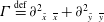 $\unicode[STIX]{x1D6E4}\stackrel{\text{def}}{=}\unicode[STIX]{x2202}_{~\tilde{x}~\overline{x}}^{2}+\unicode[STIX]{x2202}_{~{\tilde{y}}~\overline{y}}^{2}$
, and operators with tildes and overbars indicate differentiation with respect to
 $\tilde{\boldsymbol{x}}=\boldsymbol{x}_{a}-\boldsymbol{x}_{b}$
and
 $\overline{\boldsymbol{x}}=(\boldsymbol{x}_{a}+\boldsymbol{x}_{b})/2$
respectively.
Because of the statistical homogeneity of the equilibrium state, the eigenfunctions are sinusoidal. The coherent flow component of the eigenfunctions and the covariance component are given by (4.1) and (4.2) respectively. Inserting the eigenfunction into (A 3)–(A 6), we determine the perturbation covariance amplitudes in terms of the amplitudes of the perturbation mean flow. They are given by:
 $$\begin{eqnarray}{\hat{S}}^{\unicode[STIX]{x1D713}\unicode[STIX]{x1D713}}=\frac{a_{\unicode[STIX]{x1D713}}\hat{\boldsymbol{z}}\boldsymbol{\cdot }(\boldsymbol{k}_{+}\times \boldsymbol{n})k_{+}^{2}(k_{+}^{2}-N^{2}){\hat{S}}_{E+}^{\unicode[STIX]{x1D713}\unicode[STIX]{x1D713}}}{(\unicode[STIX]{x1D70E}+2)k_{+}^{2}k_{-}^{2}+\text{i}\unicode[STIX]{x1D6FD}(k_{x-}k_{+}^{2}-k_{x+}k_{-}^{2})}-\frac{a_{\unicode[STIX]{x1D713}}\hat{\boldsymbol{z}}\boldsymbol{\cdot }(\boldsymbol{k}_{-}\times \boldsymbol{n})k_{-}^{2}(k_{-}^{2}-N^{2}){\hat{S}}_{E-}^{\unicode[STIX]{x1D713}\unicode[STIX]{x1D713}}}{(\unicode[STIX]{x1D70E}+2)k_{+}^{2}k_{-}^{2}+\text{i}\unicode[STIX]{x1D6FD}(k_{x-}k_{+}^{2}-k_{x+}k_{-}^{2})},\end{eqnarray}$$
 $$\begin{eqnarray}{\hat{S}}^{\unicode[STIX]{x1D713}\unicode[STIX]{x1D703}}=\frac{a_{\unicode[STIX]{x1D703}}\hat{\boldsymbol{z}}\boldsymbol{\cdot }(\boldsymbol{k}_{+}\times \boldsymbol{n})k_{+}^{2}(k_{+}^{2}-n_{\unicode[STIX]{x1D706}}^{2}){\hat{S}}_{E+}^{\unicode[STIX]{x1D713}\unicode[STIX]{x1D713}}}{(\unicode[STIX]{x1D70E}+2)k_{+}^{2}k_{\unicode[STIX]{x1D706}-}^{2}+\text{i}\unicode[STIX]{x1D6FD}(k_{x-}k_{+}^{2}-k_{x+}k_{\unicode[STIX]{x1D706}-}^{2})}-\frac{a_{\unicode[STIX]{x1D703}}\hat{\boldsymbol{z}}\boldsymbol{\cdot }(\boldsymbol{k}_{-}\times \boldsymbol{n})k_{\unicode[STIX]{x1D706}-}^{2}(k_{-}^{2}-n^{2}){\hat{S}}_{E-}^{\unicode[STIX]{x1D703}\unicode[STIX]{x1D703}}}{(\unicode[STIX]{x1D70E}+2)k_{+}^{2}k_{\unicode[STIX]{x1D706}-}^{2}+\text{i}\unicode[STIX]{x1D6FD}(k_{x-}k_{+}^{2}-k_{x+}k_{\unicode[STIX]{x1D706}-}^{2})},\end{eqnarray}$$
 $$\begin{eqnarray}{\hat{S}}^{\unicode[STIX]{x1D703}\unicode[STIX]{x1D713}}=\frac{a_{\unicode[STIX]{x1D703}}\hat{\boldsymbol{z}}\boldsymbol{\cdot }(\boldsymbol{k}_{+}\times \boldsymbol{n})k_{\unicode[STIX]{x1D706}+}^{2}(k_{+}^{2}-n^{2}){\hat{S}}_{E+}^{\unicode[STIX]{x1D703}\unicode[STIX]{x1D703}}}{(\unicode[STIX]{x1D70E}+2)k_{\unicode[STIX]{x1D706}+}^{2}k_{-}^{2}+\text{i}\unicode[STIX]{x1D6FD}(k_{x-}k_{\unicode[STIX]{x1D706}+}^{2}-k_{x+}k_{-}^{2})}-\frac{a_{\unicode[STIX]{x1D703}}\hat{\boldsymbol{z}}\boldsymbol{\cdot }(\boldsymbol{k}_{-}\times \boldsymbol{n})k_{-}^{2}(k_{-}^{2}-n_{\unicode[STIX]{x1D706}}^{2}){\hat{S}}_{E-}^{\unicode[STIX]{x1D713}\unicode[STIX]{x1D713}}}{(\unicode[STIX]{x1D70E}+2)k_{\unicode[STIX]{x1D706}+}^{2}k_{-}^{2}+\text{i}\unicode[STIX]{x1D6FD}(k_{x-}k_{\unicode[STIX]{x1D706}+}^{2}-k_{x+}k_{-}^{2})},\end{eqnarray}$$
 $$\begin{eqnarray}{\hat{S}}^{\unicode[STIX]{x1D703}\unicode[STIX]{x1D703}}=\frac{a_{\unicode[STIX]{x1D713}}\hat{\boldsymbol{z}}\boldsymbol{\cdot }(\boldsymbol{k}_{+}\times \boldsymbol{n})k_{\unicode[STIX]{x1D706}+}^{2}(k_{\unicode[STIX]{x1D706}+}^{2}-n^{2}){\hat{S}}_{E+}^{\unicode[STIX]{x1D703}\unicode[STIX]{x1D703}}}{(\unicode[STIX]{x1D70E}+2)k_{\unicode[STIX]{x1D706}+}^{2}k_{\unicode[STIX]{x1D706}-}^{2}+\text{i}\unicode[STIX]{x1D6FD}(k_{x-}k_{\unicode[STIX]{x1D706}+}^{2}-k_{x+}k_{\unicode[STIX]{x1D706}-}^{2})}-\frac{a_{\unicode[STIX]{x1D713}}\hat{\boldsymbol{z}}\boldsymbol{\cdot }(\boldsymbol{k}_{-}\times \boldsymbol{n})k_{\unicode[STIX]{x1D706}-}^{2}(k_{\unicode[STIX]{x1D706}-}^{2}-n^{2}){\hat{S}}_{E-}^{\unicode[STIX]{x1D703}\unicode[STIX]{x1D703}}}{(\unicode[STIX]{x1D70E}+2)k_{\unicode[STIX]{x1D706}+}^{2}k_{\unicode[STIX]{x1D706}-}^{2}+\text{i}\unicode[STIX]{x1D6FD}(k_{x-}k_{\unicode[STIX]{x1D706}+}^{2}-k_{x+}k_{\unicode[STIX]{x1D706}-}^{2})},\end{eqnarray}$$
 $\boldsymbol{k}_{\pm }=\boldsymbol{k}\pm \boldsymbol{n}/2$
,
 $k_{\pm }^{2}=|\boldsymbol{k}_{\pm }|^{2}$
,
 $k_{\unicode[STIX]{x1D706}\pm }^{2}=|\boldsymbol{k}_{\pm }|^{2}+2\unicode[STIX]{x1D706}^{2}$
,
 $n_{\unicode[STIX]{x1D706}}=n^{2}+2\unicode[STIX]{x1D706}^{2}$
,
 ${\hat{S}}_{E\pm }^{\unicode[STIX]{x1D713}\unicode[STIX]{x1D713}}(\boldsymbol{k})=(1+p)\hat{\unicode[STIX]{x1D6EF}}(\boldsymbol{k}_{\pm })/2k_{\pm }^{4}$
,
 ${\hat{S}}_{E\pm }^{\unicode[STIX]{x1D703}\unicode[STIX]{x1D703}}(\boldsymbol{k})=(1-p)\hat{\unicode[STIX]{x1D6EF}}(\boldsymbol{k}_{\pm })/2k_{\unicode[STIX]{x1D706}\pm }^{4}$
and
 $\hat{\boldsymbol{z}}$
the unit vector representing the vertical direction.
The perturbation eddy stress divergences can then be determined as a function of the perturbation coherent flow and the spectrum of the excitation. They are:
 $$\begin{eqnarray}[\unicode[STIX]{x1D6FF}f_{\unicode[STIX]{x1D713}},\unicode[STIX]{x1D6FF}f_{\unicode[STIX]{x1D703}}]^{\text{T}}=[a_{\unicode[STIX]{x1D713}}(f_{\unicode[STIX]{x1D713}\unicode[STIX]{x1D713}+}-f_{\unicode[STIX]{x1D713}\unicode[STIX]{x1D713}-}),a_{\unicode[STIX]{x1D703}}(f_{\unicode[STIX]{x1D703}\unicode[STIX]{x1D703}+}-f_{\unicode[STIX]{x1D703}\unicode[STIX]{x1D703}-})]^{\text{T}}\text{e}^{\text{i}\boldsymbol{n}\boldsymbol{\cdot }\boldsymbol{x}},\end{eqnarray}$$
where
 $$\begin{eqnarray}\displaystyle f_{\unicode[STIX]{x1D713}\unicode[STIX]{x1D713}\pm } & = & \displaystyle \frac{1}{4\unicode[STIX]{x03C0}}\int _{-\infty }^{\infty }\int _{-\infty }^{\infty }\frac{\hat{\boldsymbol{z}}\boldsymbol{\cdot }[k_{+}^{2}(\boldsymbol{k}_{-}\times \boldsymbol{n})-k_{-}^{2}(\boldsymbol{k}_{+}\times \boldsymbol{n})]\hat{\boldsymbol{z}}\boldsymbol{\cdot }(\boldsymbol{k}_{\pm }\times \boldsymbol{n})k_{\unicode[STIX]{x1D706}\pm }^{2}(k_{\unicode[STIX]{x1D706}\pm }^{2}-n^{2}){\hat{S}}_{E\pm }^{\unicode[STIX]{x1D703}\unicode[STIX]{x1D703}}}{(\unicode[STIX]{x1D70E}+2)k_{\unicode[STIX]{x1D706}+}^{2}k_{\unicode[STIX]{x1D706}-}^{2}+\text{i}\unicode[STIX]{x1D6FD}(k_{x-}k_{\unicode[STIX]{x1D706}+}^{2}-k_{x+}k_{\unicode[STIX]{x1D706}-}^{2})}\,\text{d}^{2}\boldsymbol{k}\nonumber\\ \displaystyle & & \displaystyle +\,\frac{1}{4\unicode[STIX]{x03C0}}\int _{-\infty }^{\infty }\int _{-\infty }^{\infty }\frac{\hat{\boldsymbol{z}}\boldsymbol{\cdot }[k_{+}^{2}(\boldsymbol{k}_{-}\times \boldsymbol{n})-k_{-}^{2}(\boldsymbol{k}_{+}\times \boldsymbol{n})]\hat{\boldsymbol{z}}\boldsymbol{\cdot }(\boldsymbol{k}_{\pm }\times \boldsymbol{n})k_{\pm }^{2}(k_{\pm }^{2}-N^{2}){\hat{S}}_{E\pm }^{\unicode[STIX]{x1D713}\unicode[STIX]{x1D713}}}{(\unicode[STIX]{x1D70E}+2)k_{+}^{2}k_{-}^{2}+\text{i}\unicode[STIX]{x1D6FD}(k_{x-}k_{+}^{2}-k_{x+}k_{-}^{2})}\,\text{d}^{2}\boldsymbol{k},\nonumber\\ \displaystyle & & \displaystyle\end{eqnarray}$$
 $$\begin{eqnarray}\displaystyle f_{\unicode[STIX]{x1D703}\unicode[STIX]{x1D703}\pm } & = & \displaystyle \frac{1}{4\unicode[STIX]{x03C0}}\int _{-\infty }^{\infty }\int _{-\infty }^{\infty }\frac{\hat{\boldsymbol{z}}\boldsymbol{\cdot }[-k_{\unicode[STIX]{x1D706}\mp }^{2}(\boldsymbol{k}_{\pm }\times \boldsymbol{n})+k_{\pm }^{2}(\boldsymbol{k}_{\mp }\times \boldsymbol{n})]\hat{\boldsymbol{z}}\boldsymbol{\cdot }(\boldsymbol{k}_{\pm }\times \boldsymbol{n})k_{\pm }^{2}(k_{\pm }^{2}-n_{\unicode[STIX]{x1D706}}^{2}){\hat{S}}_{E\pm }^{\unicode[STIX]{x1D713}\unicode[STIX]{x1D713}}}{(\unicode[STIX]{x1D70E}+2)k_{+}^{2}k_{\unicode[STIX]{x1D706}-}^{2}+\text{i}\unicode[STIX]{x1D6FD}(k_{x-}k_{+}^{2}-k_{x+}k_{\unicode[STIX]{x1D706}-}^{2})}\,\text{d}^{2}\boldsymbol{k}\nonumber\\ \displaystyle & & \displaystyle +\,\frac{1}{4\unicode[STIX]{x03C0}}\int _{-\infty }^{\infty }\!\int _{-\infty }^{\infty }\!\frac{\hat{\boldsymbol{z}}\boldsymbol{\cdot }[-k_{\mp }^{2}(\boldsymbol{k}_{\pm }\times \boldsymbol{n})+k_{\unicode[STIX]{x1D706}\pm }^{2}(\boldsymbol{k}_{\mp }\times \boldsymbol{n})]\hat{\boldsymbol{z}}\boldsymbol{\cdot }(\boldsymbol{k}_{\pm }\times \boldsymbol{n})k_{\unicode[STIX]{x1D706}\pm }^{2}(k_{\pm }^{2}-n^{2}){\hat{S}}_{E\pm }^{\unicode[STIX]{x1D703}\unicode[STIX]{x1D703}}}{(\unicode[STIX]{x1D70E}+2)k_{\unicode[STIX]{x1D706}+}^{2}k_{-}^{2}+\text{i}\unicode[STIX]{x1D6FD}(k_{x-}k_{\unicode[STIX]{x1D706}+}^{2}-k_{x+}k_{-}^{2})}\,\text{d}^{2}\boldsymbol{k}.\nonumber\\ \displaystyle & & \displaystyle\end{eqnarray}$$
Note that when there is no correlation of the barotropic and the baroclinic streamfunction at equilibrium (
 $S_{E}^{\unicode[STIX]{x1D713}\unicode[STIX]{x1D703}}=S_{E}^{\unicode[STIX]{x1D703}\unicode[STIX]{x1D713}}=0$
), perturbations to the homogeneous equilibrium with no temperature difference across the channel have the property that barotropic mean flow perturbations induce only barotropic mean-flow accelerations and baroclinic mean flow perturbations induce only baroclinic mean-flow accelerations decoupling the barotropic and baroclinic mean-flow tendencies.
A further reduction in the above expressions can be achieved, as noted by Srinivasan & Young (Reference Srinivasan and Young2012), by utilizing the exchange symmetry of the covariance
 $\unicode[STIX]{x1D63E}(\boldsymbol{x}_{a},\boldsymbol{x}_{b})=\unicode[STIX]{x1D63E}(\boldsymbol{x}_{b},\boldsymbol{x}_{a})^{\text{T}}$
, by changing the sign of
 $\boldsymbol{k}$
in the integrals to obtain
 $$\begin{eqnarray}f_{\unicode[STIX]{x1D713}\unicode[STIX]{x1D713}+}=-f_{\unicode[STIX]{x1D713}\unicode[STIX]{x1D713}-},\quad f_{\unicode[STIX]{x1D703}\unicode[STIX]{x1D703}+}=-f_{\unicode[STIX]{x1D703}\unicode[STIX]{x1D703}-}.\end{eqnarray}$$
Introduction of (A 11a,b
) into (A 8) and the change of variables
 $\boldsymbol{k}\rightarrow \boldsymbol{k}+\boldsymbol{n}/2$
, in the integrals yields the more compact representation of the eddy stress divergences:
 $$\begin{eqnarray}[\unicode[STIX]{x1D6FF}f_{\unicode[STIX]{x1D713}},\unicode[STIX]{x1D6FF}f_{\unicode[STIX]{x1D703}}]^{\text{T}}=[a_{\unicode[STIX]{x1D713}}f_{\unicode[STIX]{x1D713}}(\unicode[STIX]{x1D70E}),a_{\unicode[STIX]{x1D703}}f_{\unicode[STIX]{x1D703}}(\unicode[STIX]{x1D70E})]^{\text{T}}\text{e}^{\text{i}\boldsymbol{n}\boldsymbol{\cdot }\boldsymbol{x}},\end{eqnarray}$$
with
 $f_{\unicode[STIX]{x1D713}}(\unicode[STIX]{x1D70E})$
and
 $f_{\unicode[STIX]{x1D703}}(\unicode[STIX]{x1D70E})$
being given by (4.5) and (4.6) respectively. Because the barotropic and baroclinic perturbation components decouple upon substitution of (A 12) in (A 2) we obtain that either
 $\unicode[STIX]{x1D70E}$
satisfies (4.3) and the eigenfunction is purely barotropic with
 $a_{\unicode[STIX]{x1D713}}\neq 0$
and
 $a_{\unicode[STIX]{x1D703}}=0$
, or that
 $\unicode[STIX]{x1D70E}$
satisfies (4.4) and the eigenfunction is purely baroclinic with
 $a_{\unicode[STIX]{x1D713}}=0$
and
 $a_{\unicode[STIX]{x1D703}}\neq 0$
.