

Introduction
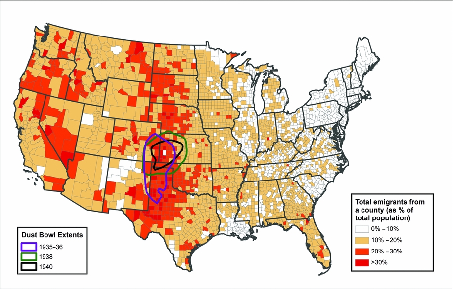
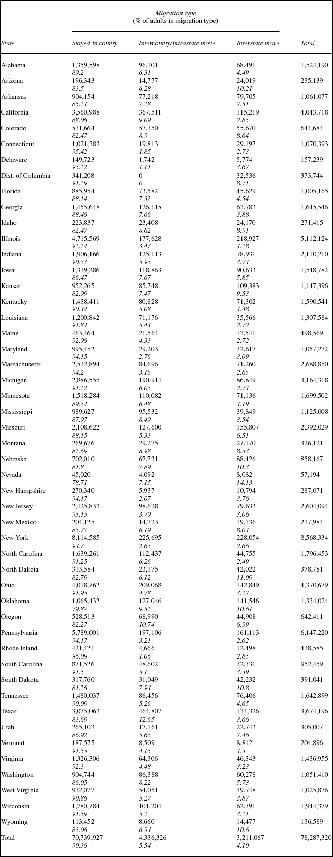
People on the move are an enduring image of the United States in the 1930s, from photographs (Agee and Evans Reference Agee and Evans1941), literature (Steinbeck Reference Steinbeck1939), and history (Egan Reference Egan2006; Gregory Reference Gregory1989). People did move in the 1930s, spurred by the economic difficulties of the Great Depression, by heat and drought, and by a multitude of other pressures. The scale of migration in the 1930s is visible in figure 1, which shows the rate of out-migration from counties between 1935 and 1940, and in table 1, which shows out-migration rates for states, divided into moves across county boundaries within states, and those that crossed state boundaries.Footnote 1 Figure 1 also outlines the area usually recognized as the extent of the dust storm activity in the 1930s and 1940, which provides a sense of ways that weather and agricultural stress acted on the lives of US residents in this era.Footnote 2
Total emigrants from county, 1935–1940, as a percentage of total estimated 1935 county population.
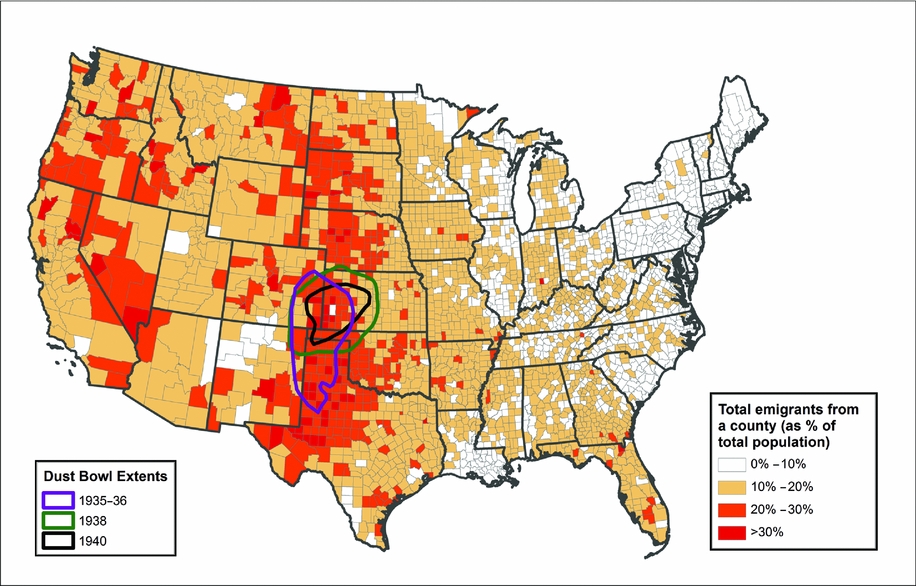
Estimated adult domestic migration by 1935 state of residence
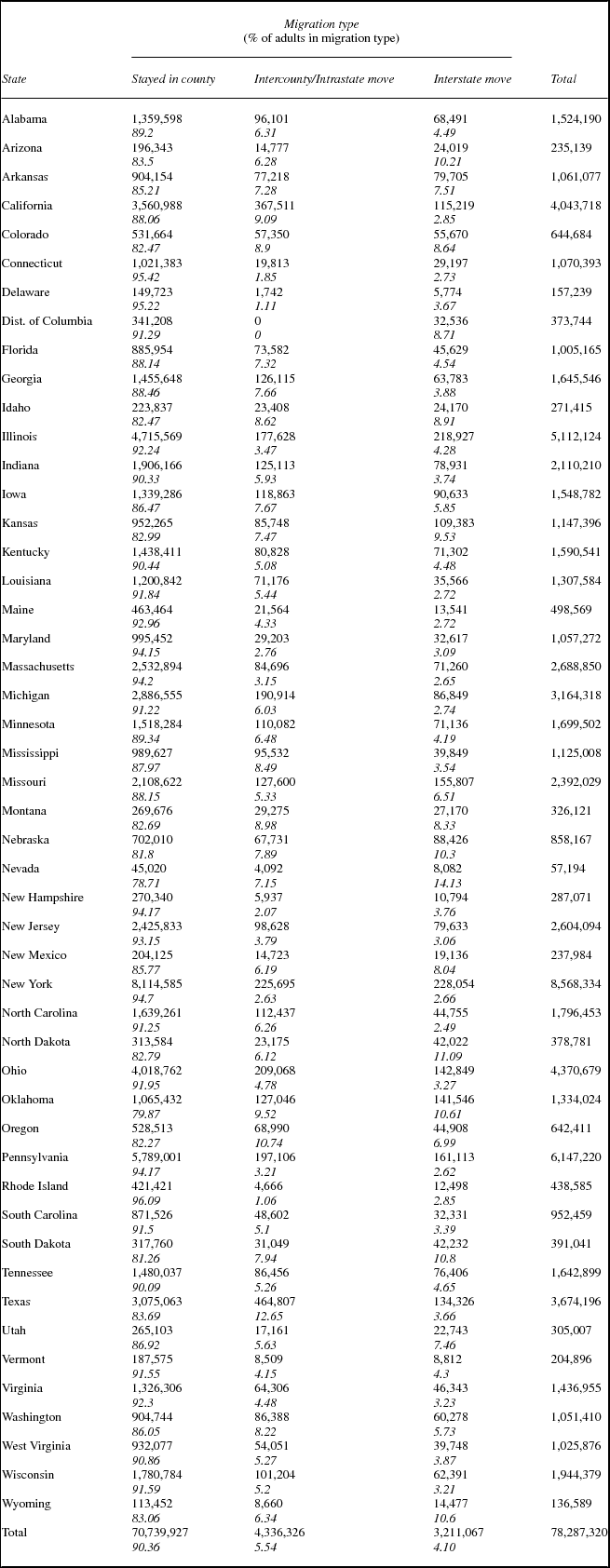
Despite the lore of the Dust Bowl and the “Great Migration” from the South to the North, the volume of internal US state-to-state migration was not all that great from the early twentieth century until after World War II (US Bureau of the Census 1946). Modest interstate migration rates belie a continuing mobility made up of streams of people moving relatively short distances from one type of community to another (Bogue et al. Reference Bogue, Shryock and Hoermann1957; Ferrie Reference Ferrie, Carter, Gartner, Haines, Olmstead, Sutch and Wright2006; Hall and Ruggles Reference Hall and Ruggles2004; US Bureau of the Census 1946). In addition, as figure 1 shows, areas with substantial out-migration were not limited to the Dust Bowl or the Deep South. Nonetheless, migration was a frequent subject of discussion, important enough that the US Census tracked migration for the first time in 1940, asking exactly where every person enumerated had lived five years earlier (US Bureau of the Census 2002). With this wealth of data, research about migration in the 1930s has explored many questions but left even more unanswered (Bogue and Hagood Reference Bogue and Hagood1953; Bogue et al. Reference Bogue, Shryock and Hoermann1957; Boustan et al. Reference Boustan, Price, Fishback and Kantor2010, Reference Boustan, Kahn and Rhode2012; Fishback et al. Reference Fishback, Horrace and Kantor2006; Hornbeck Reference Hornbeck2012; Lively and Taeuber Reference Lively and Taeuber1939; Long and Siu Reference Long and Siu2013; McLeman Reference McLeman2013; McLeman and Smit Reference McLeman and Smit2006; Tolnay et al. Reference Tolnay, White, Crowder and Adelman2005; US Bureau of the Census 1946; White Reference White2005; White et al. Reference White, Crowder, Tolnay and Adelman2005).
How much do we really know about the causes of migration in the 1930s? To what extent do we know that the big forces that are supposed to have been important actually were significant? This is an important question, and the availability of census data for 1940 that shows where virtually every American lived in 1935 makes it possible to think about the factors that drove migration at a very refined scale. Moreover, the availability of data about weather, agriculture, and employment—among other factors—with comparable refinement make it possible to add real insight to our understanding. Unlike previously utilized sample or tabulated population data they show the migration experience of almost every American resident at the county level, and tell us where they went (although for this article we are only interested in whether they moved across county or state lines). Managing these detailed and complex data—there were more than 130 million American inhabitants in 1940—created significant challenges, and describing how we overcame those challenges constitutes a significant part of this article. However, our findings are important as well.
To a great extent, the conventional story of the 1930s is right but too limiting: People left areas where the weather was challenging for agriculture in the mid-1930s, but that experience was not limited to the Dust Bowl region. The weather was hot and dry in a much larger part of the United States, and migrants escaped those areas as well. Moreover, much more was happening. There were regional processes that intensified the agriculture and weather effects, and broader economic processes that are predictable. Our research confirms much that we should have known all along, but with much more detailed data that give us confidence that we understand what was happening.
Theoretical Background
A large theoretical literature (Greenwood Reference Greenwood, Mark and Oded1997; Lee Reference Lee1966; Massey Reference Massey1990; Massey et al. Reference Massey, Arango, Hugo, Kouaouci, Pellegrino and Taylor1998; Ravenstein Reference Ravenstein1885, Reference Ravenstein1889; Roy Reference Roy1951) has sought to explain migration. Though much of it focuses on international migration, its core elements have also been applied to internal migration. Neoclassical economics provides the dominant perspective, informed by contributions from the New Economics of Migration, by Massey's notion of Cumulative Causation Theory and by the descriptive richness of Migration Systems Theory (Bakewell Reference Bakewell2013; Fussell et al. Reference Fussell, Curtis and DeWaard2014; Massey Reference Massey1990; Massey, et al. Reference Massey, Arango, Hugo, Kouaouci, Pellegrino and Taylor1993). In these approaches, a person's likelihood of migrating is a function of not only his or her individual characteristics but also of the characteristics of their places of origin and destination, including the distribution of income, land, and human capital; the organization of agriculture and industry; public policy; and cultural frameworks, reflected in local ethnic, religious, and racial conditions (Fishback et al. Reference Fishback, Horrace and Kantor2006; Massey et al. Reference Massey, Arango, Hugo, Kouaouci, Pellegrino and Taylor1993). The structure of social networks shapes migration. Because these processes are not independent of spatial context, we see migration not merely as people moving in unconnected and location-free contexts but as interactions between people and locations following specific pathways.
Most research sees migration as a tension between pushes and pulls, and theorizes that migration serves as a mechanism to restore equilibrium between competing forces. Disaster-related demographic theory builds on these patterns of movement to identify the migratory systems that existed prior to the disaster and to gauge whether a given shock transforms the preexisting migration system (Black et al. Reference Black, Adger, Arnell, Dercon, Geddes and Thomas2011; Fussell et al. Reference Fussell, Curtis and DeWaard2014; McLeman Reference McLeman2013). The disaster literature also adds the concept of vulnerability to the determinants of migration (Adger Reference Adger2006; McLeman Reference McLeman2013; McLeman and Smit Reference McLeman and Smit2006). The vulnerability paradigm focuses on the exposure of people to stress over time, prior to the period of crisis, based on the condition of the economic and ecological systems they inhabit. Assessments of vulnerability have focused on both short-term moves and long-term reorganizations of human-environment systems (Adger Reference Adger2006; Berkes et al. Reference Berkes, Carl and Johan1998; Black et al. Reference Black, Arnell, Adger, Thomas and Geddes2013), asking whether a specific “demographic signature of disaster” exists (DeWaard et al. Reference DeWaard, Curtis and Fussell2014). In the United States, the Dust Bowl story has driven research about environmental migration in the 1930s, yet drought and land degradation were not limited to the southern plains. Extreme heat also led to agricultural stress elsewhere (Giesen Reference Giesen2011; Gregory Reference Gregory2005; McEwan et al. Reference McEwan, Pederson, Cooper, Taylor, Watts and Hruska2014; Olmstead and Rhode Reference Olmstead and Rhode2008).
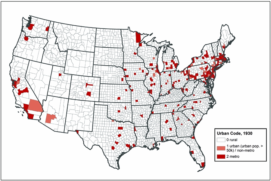
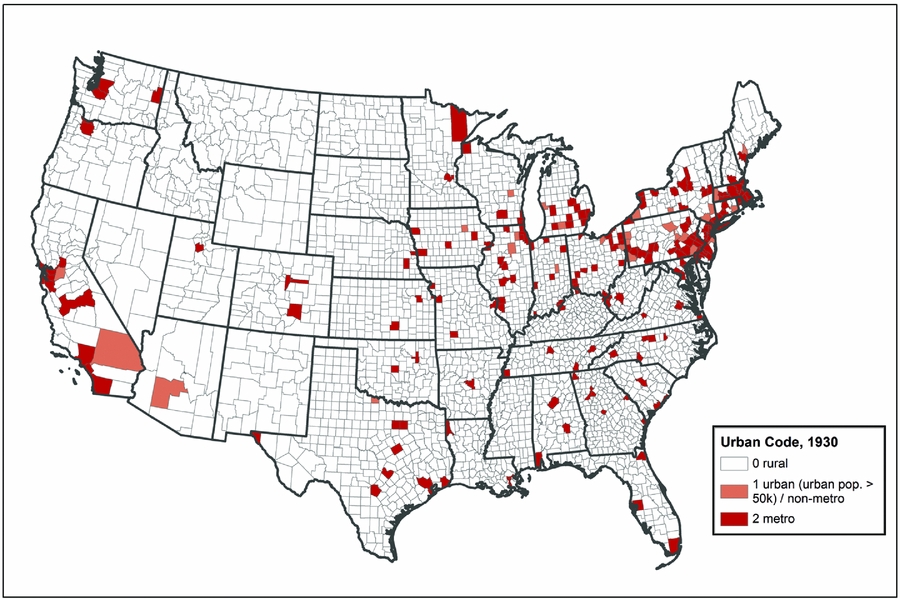
Our analysis is not limited to environmentally driven agricultural shocks. The United States was in the midst of a depression in the 1930s, with high unemployment, low wages, and a weak economic recovery. We also ask whether people left places with comparatively poor economic conditions, or stayed in places with relatively good economic conditions, and did so in a way that reveals the characteristics of places as drivers of migration. The United States still had a significant rural population in the 1930s, with more than 40 percent of its inhabitants living in places of less than 2,500 residents in both 1930 and 1940 (US Bureau of the Census 2012). The West, South, and Midwest were significantly more rural, while the Northeast was significantly less rural. Farming was still a major industry in many parts of the country, and weather had a major impact on agriculture and, consequently, the rural economy. The limits of urbanization are visible in figure 2, which shows where all the counties that had an urban population of 50,000 or more were located. The map is sparse.
Counties by urban code, 1930.
For the analysis reported here, we focus on the attributes of counties rather than the attributes of individuals. We are interested in how likely it was for someone living in a given US county in 1935 to migrate to another county by the time of the 1940 Census, and the attributes of counties that made them more or less likely to send their inhabitants elsewhere by 1940. We realize that this is a substantial simplification, because the migration literature is heavily focused on the idea first raised by Roy (Reference Roy1951) that migrants self-select for upward mobility. Moreover, Borjas (Reference Borjas1987) expanded selection theory by arguing that it is the more highly skilled who migrate, and Kanbur and Rapoport (Reference Kanbur and Rapoport2005) argue that selectivity by education is key. While we recognize that individual attributes are as important as those of context in determining who migrates, from which communities, and where they go, our approach is an important first step in understanding how migration operated in this era, and how county characteristics shaped out-migration flows.
Understanding Relative Levels of Out-migration
The main questions we explore revolve around the role of the environment and economy in encouraging or discouraging out-migration from counties between 1935 and 1940. We discuss the data that we rely on, and questions raised by the nature of those data, in a later section. We begin by discussing the factors that may have led one county to experience more out-migration than another. Our focus is mostly on processes that are important for the less urbanized parts of the United States, where natural phenomena, such as precipitation and temperature, may have had a strong effect, either acting on their own or acting through agriculture. We also include measures related to employment by industry and unemployment, which we hypothesize play a role in determining migration even in urban areas. While other researchers have examined the role of New Deal support programs in explaining migration (Fishback et al. Reference Fishback, Horrace and Kantor2006), our preliminary analysis suggested that they were less important than other factors, and they are not included in our statistical models.
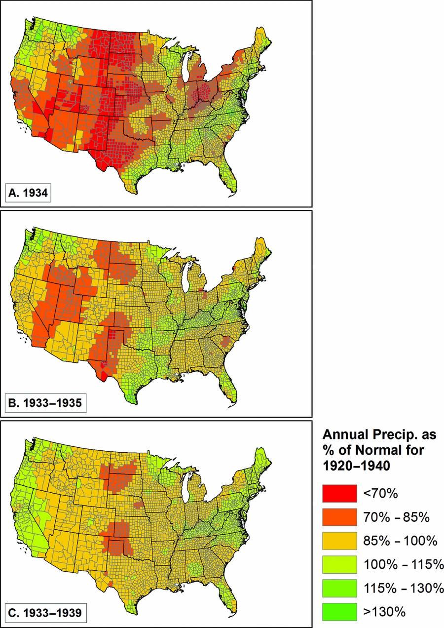
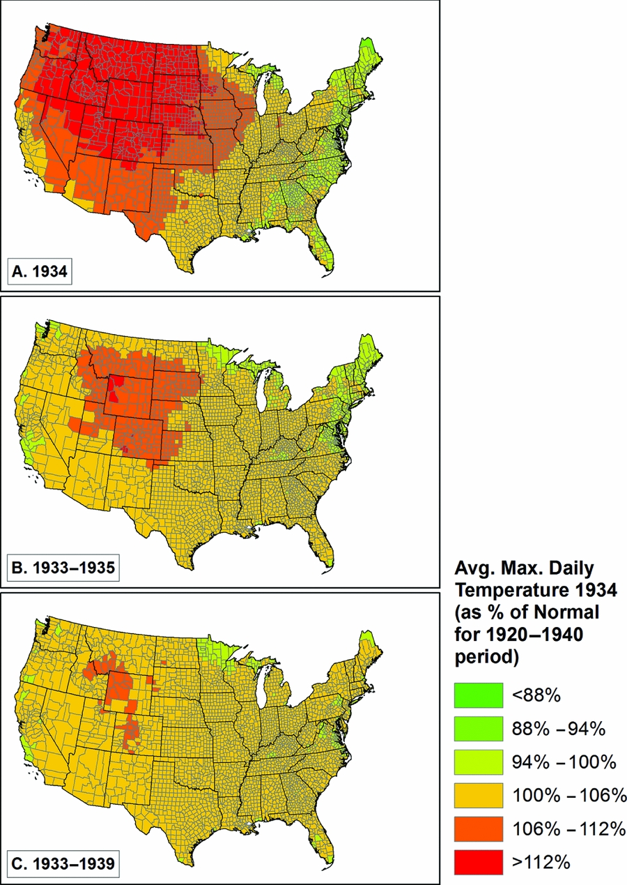
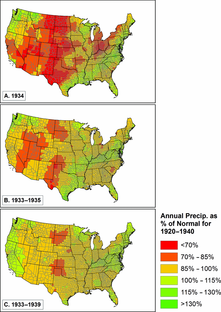
Given the severe drought of the mid-1930s, which has been described recently as the worst drought of the last millennium (Cook et al. Reference Cook, Seager and Smerdon2014), we begin with an examination of the role of weather in influencing levels of out-migration from US counties. We measure weather by looking at annual total precipitation for various time periods, and average daily maximum temperature as a percentage of a longer term (1920–40) average. The drought was worst in 1934 (and to some extent similarly severe in 1933 and 1935), so we have created relative weather measures for 1934, 1933–35, and 1933–39. We show the scale of the drought for these time periods in figures 3 and 4. Both temperature (higher than normal) and precipitation (lower than normal) diverged most significantly from expected patterns in 1934, somewhat less so in 1933–35, and came closer to normal for the seven-year period from 1933 to 1939. What is also clear is that the spatial patterns were rather different, with the highest sustained temperatures in the front range of the Rocky Mountains and the northwestern Great Plains (see especially figure 4.b), and the lowest sustained precipitation in the classic Dust Bowl areas in Oklahoma, Texas, Kansas, New Mexico, and Colorado, plus parts of the northern plains (figure 3.c), and to a lesser extent in the intermountain west (California, Nevada, Utah, Wyoming, and Idaho; figure 3.b).
Annual precipitation as a percentage of the 1920 to 1940 average.
Annual daily maximum temperature as a percentage of the 1920 to 1940 average.

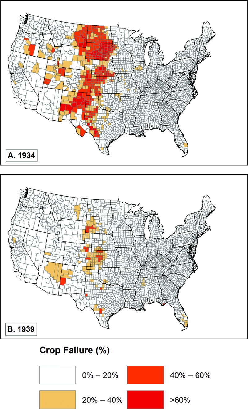
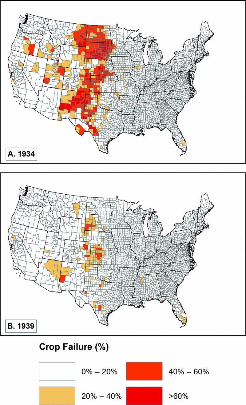
We utilize a variety of ways to measure changes in agriculture during the 1930s, making use of data from the 1930, 1935, and 1940 censuses of agriculture, which represent agricultural results in 1929, 1934, and 1939, respectively (Haines et al. Reference Haines, Price, Fishback and Rhode2014). The agricultural census includes one direct measure, the percent of land with failed crops. We display this in figure 5. The two panels of the figure show the consequences of the most severe weather, with significant failure levels throughout the central United States in 1934, and in areas of Kansas, Colorado, Arizona, New Mexico, and South Dakota (and spots elsewhere) in 1939.
Crop failure acreage as percentage of total crop acreage.
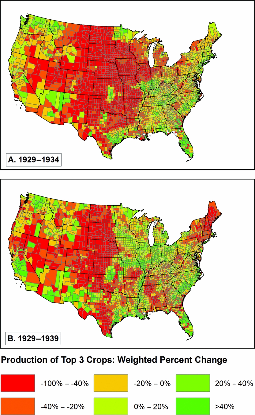
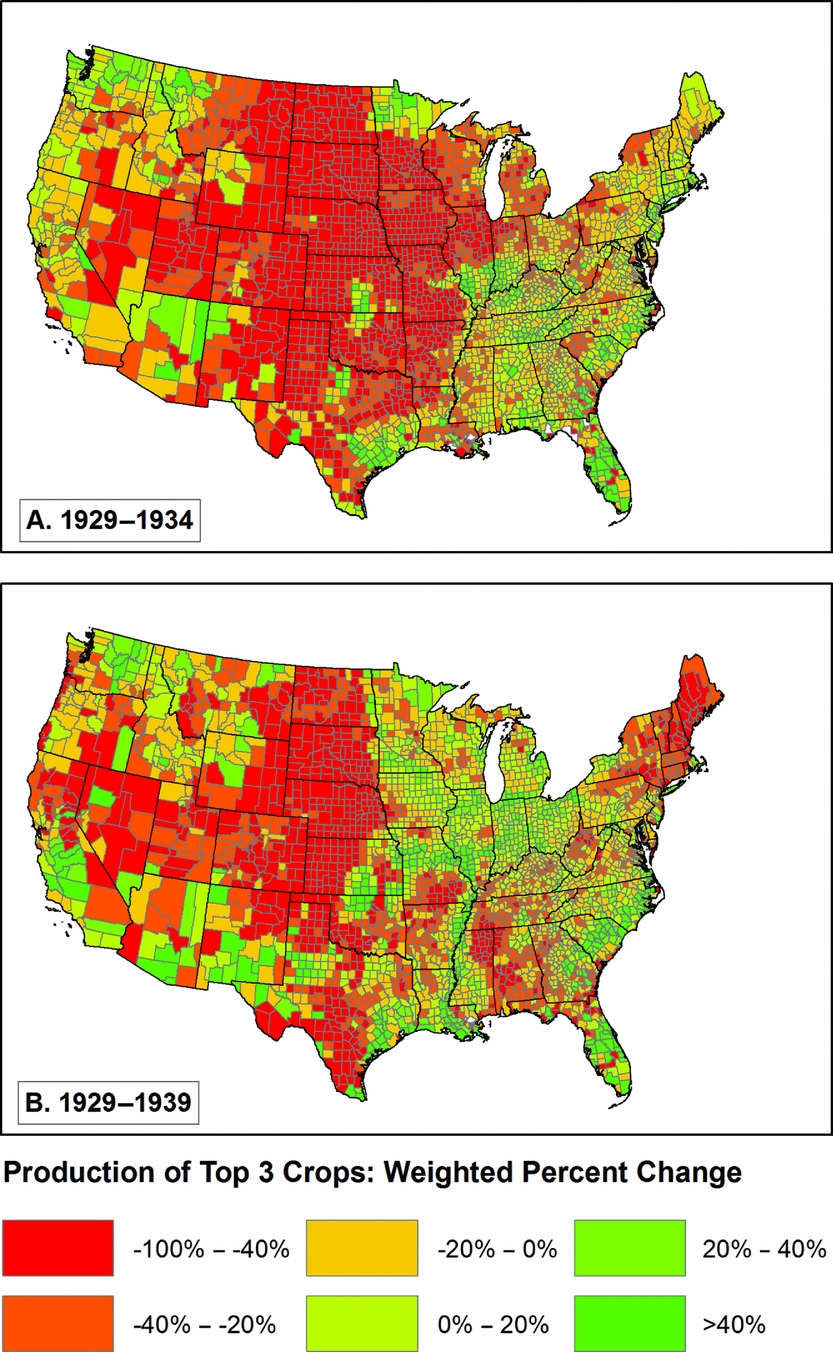
In order to attempt to find new ways to gauge the impact of the weather on agricultural production, we developed three other measures. The most ambitious of our measures estimates the percent change in crop production from 1929 to 1934 and from 1929 to 1939, for each county's three largest crops as indicated in the 1930 Census. We describe the methods we used to derive these estimates in Appendix A. This measure captures the overall falloff in production, including that due to farmers not having the resources to plant or believing that the crop would fail anyway. As we show in figure 6, a very large portion of the United States experienced major production shortfalls in 1934, something that still had not been reversed in 1939. The spatial pattern changes between 1934 and 1939, with a greater falloff in production in the later period in Georgia, Mississippi, Alabama, and Kentucky, plus New England and New York, and less in the corn belt states (Illinois, Iowa, northern Missouri), and the upper Midwest (Wisconsin, Minnesota).
Weighted percent change in county's three top crops.
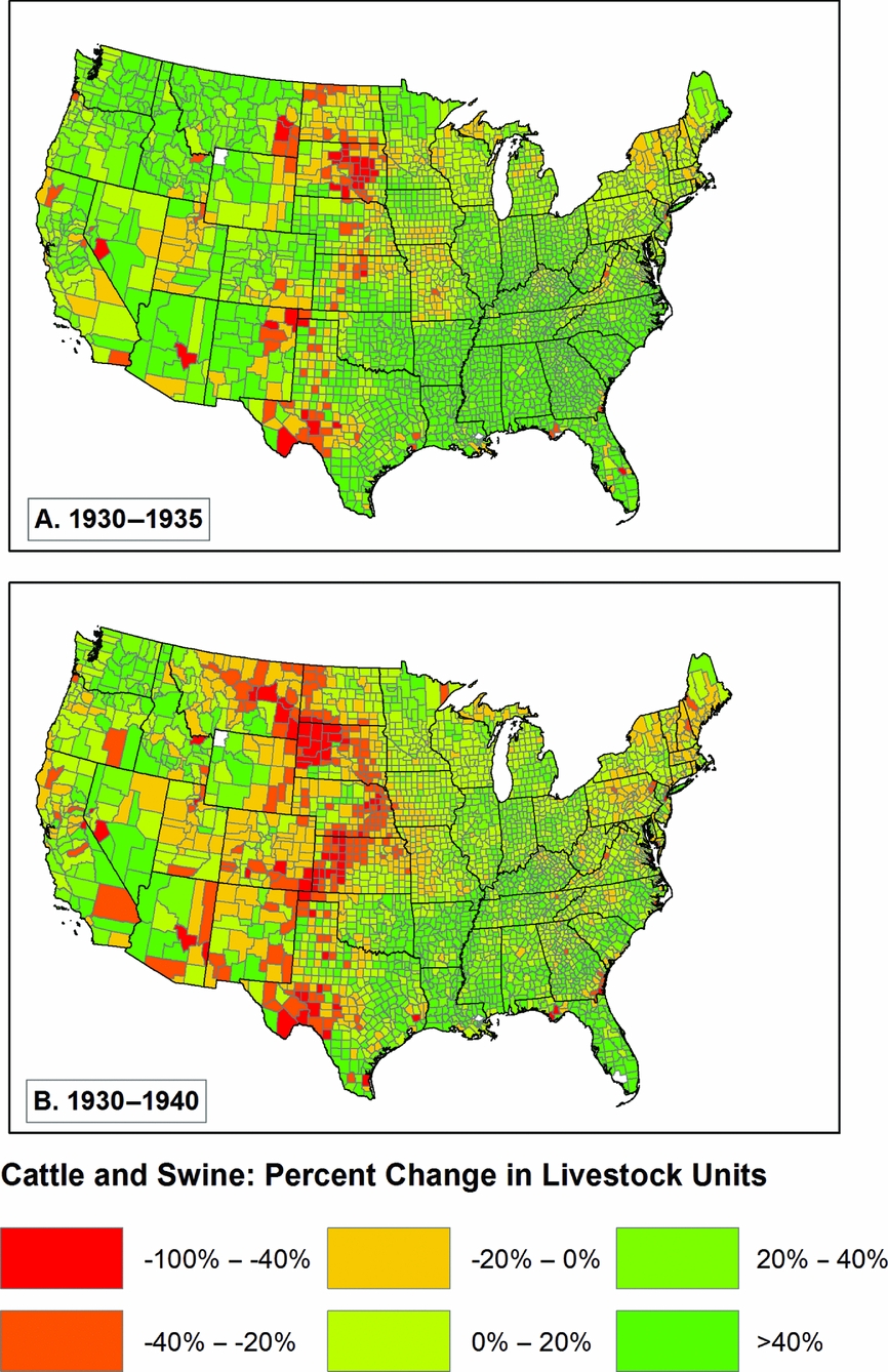
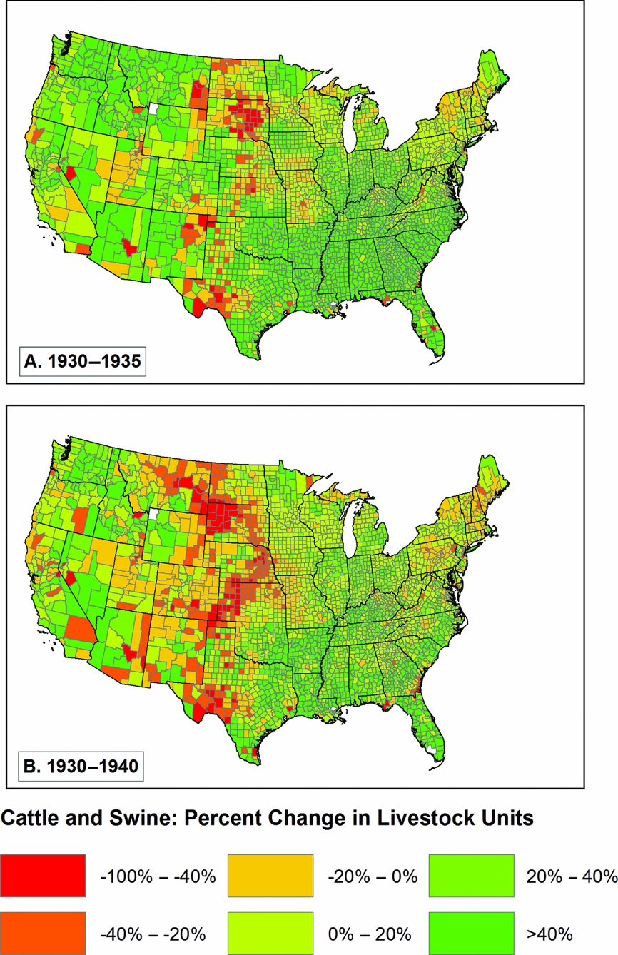
We also experimented with two other measures. In one, we made the same calculation we did for the three largest crops, and instead focused only on corn, wheat, and cotton. In a second, we attempted to gauge the impact of severe weather and poor agricultural conditions on livestock by estimating livestock inventories in 1935 and 1940 as a percentage of what they were in 1930 (figure 7b).Footnote 3 The results shown in figure 7 are interesting because they show that, in most parts of the United States, livestock had increased between 1930 and 1935 (figure 7.a), with some exceptions in areas of the central United States with the worst weather. The situation worsened between 1935 and 1940 (figure 7.b), but livestock nonetheless continued to increase in numbers in most of the country.
Percent change in cattle and swine by livestock unit (1930–35 and 1930–40).
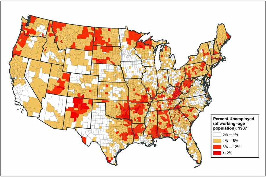
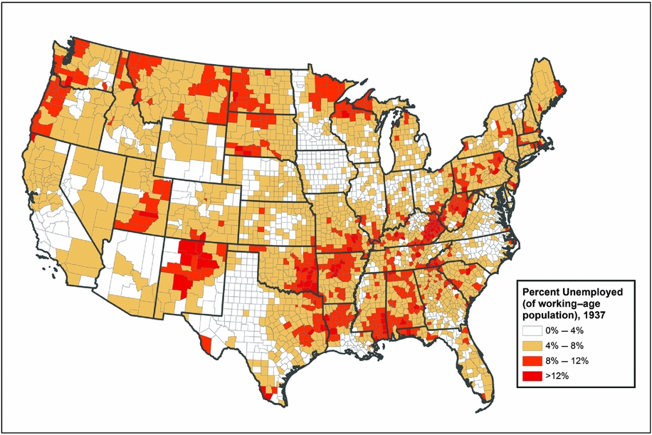
Although we hypothesize that changes in agriculture drove most of the out-migration in the 1930s, other economic factors played a role. One of these is unemployment, which was enumerated in a special census of “partial employment, unemployment, and occupations,” in 1937 (Biggers and United States Reference Biggers1938).Footnote 4 Figure 8 displays the spatial distribution of unemployment, with the highest levels of unemployment in the Deep South, Appalachia, in the northeast, along the northern tier of the United States, and in Utah and New Mexico. As we might predict this does not appear to align easily with either weather or agriculture. We believe the economy played a broader role, so we have also examined employment in various industries as a potential indicator that the economy was capable of doing better or worse in different areas of the United States, with an impact on migration.
Percent of working age population unemployed, 1937.
Our hypotheses are simple and straightforward. We expect that rural counties that experienced severe weather, poor agricultural results, and high unemployment should have had higher levels of out-migration than those that did not, and that urban counties and counties with higher levels of employment in manufacturing and retail sales should have had lower levels of out-migration, all other things being equal.
Data and Methods
The variety of data necessary for this analysis, originally gathered at different spatial and temporal scales, were transformed in order to produce a data set that may be analyzed at the county level. Our dependent variable is the rate of out-migration from each county of the United States between 1935 and 1940, based on the data in the 1940 US Census of Population. The independent variables draw on environmental, agricultural, and economic data. The methods we use include both descriptive and multivariate approaches.
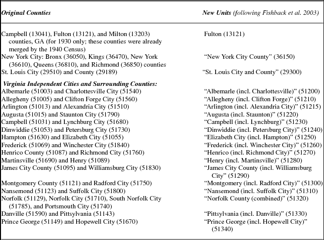
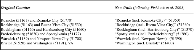
The list of counties of the United States has changed over time, even during as brief a period as the decade from 1930 to 1940. For this analysis, we began with the 1940 list of counties and their geography, and modified that geography to take into account changes in the list of counties and the ways that we and others have aggregated counties to optimize analysis. First, there are counties that existed in 1930 but not in 1940 (or vice versa). Campbell and Milton counties were merged into Fulton County, Georgia, between 1930 and 1940; we combined these three counties into one. In another case, we aggregated spatial units in Virginia in order to combine independent cities with their surrounding counties.Footnote 5 In a third modification, we needed to merge counties from a single metropolitan area where confusing naming practices made it impossible to distinguish separate counties (New York City's five counties and Saint Louis City and Saint Louis County, Missouri). These modifications are summarized in Appendix B. The resulting data set contains 3,069 counties from the contiguous 48 states that existed in 1940. In the cases in which we combined counties and the data were counts, we summed the counts across all geographic units. In the case of data that were rates or averages, we calculated means, which were spatially weighted when appropriate.
Census Data
The 1940 US Census of Population full count data have a wealth of information about individuals, including demographic, social and cultural, economic, and location data (Ruggles et al. Reference Ruggles, Alexander, Genadek, Goeken, Schroeder and Sobek2010), and constitute the primary data source for our analysis. In the 1940 Census, respondents were asked to provide their county of residence and that of all their household members in 1935. At the time we undertook this analysis, the full-count 1940 data were available in two forms, and we made use of both of them. The University of Minnesota's Integrated Public Use Microdata Series (IPUMS) project has released a preliminary version of the 1940 data in IPUMS coded format, which includes every person in the United States but not every variable from the census. The IPUMS version of the 1940 data set includes standardized variables for a person's 1935 state of residence and the scale of their residential movements since 1935, delineating those who moved within or between counties, states, and countries, but the coded data do not yet contain a variable for which county a person lived in in 1935. That information is available from a restricted release of a version of the 1940 data that does include the detailed response text for every person. We have merged these data sets, and coded—to the extent possible—origin county from the 1935 textual residence variable, in addition to recoding 1940 places of residence that were erroneously coded in the IPUMS data (e.g., coding that conflated Brown and Boone counties in Indiana, and Richmond City and Richmond County in Virginia). That turned out to be a challenging task, which we describe in Appendix C.
Table 1 presents a subset of the data, tabulated by state of residence in 1935. This allows us to show the level of out-migration from counties within states, for migrants who stayed within their state of residence (“intercounty move”) and those who left their state of residence (“interstate move”). We exclude people under age 20 in 1940, people living in group quarters in 1940, those living outside the United States in 1935, and those whose residence in 1935 is unknown. For the contiguous United States as a whole, using our data set, 5.5 percent of the population moved across county boundaries (but stayed in state),Footnote 6 and 4.1 percent moved across state lines, a total of 9.6 percent. Variation from state to state is substantial, as we would expect.
Weather and Climate Data
We derived our climatological variables from data sets developed by the PRISM Climate Group at Oregon State University. These PRISM data are 4km-grid rasters of temperature and precipitation, modeled at a monthly resolution, stretching back to the late nineteenth century, and covering the contiguous United States. Assuming that physiographic factors such as elevation and aspect have influenced local climate in a similar way in both the more recent and more distant past, the PRISM group incorporated a “climate fingerprint” from 30-year normals for 1971–2000 into their expert system to fill in the gaps between scattered weather monitoring stations for earlier years. Further details on PRISM's method of topographically informed interpolation may be found in the group's publications and web documentation (Daly et al. Reference Daly, Gibson, Taylor, Johnson and Pasteris2002, Reference Daly, Halbleib, Smith, Gibson, Doggett, Taylor, Curtis and Pasteris2008). For our analysis, we aggregated the PRISM data to counties by calculating zonal statistics, using 1940 county boundaries from the National Historical Geographical Information System, and aligned with the PRISM rasters.Footnote 7 In order to do this we averaged the grid cell values within each county to calculate the maximum and minimum temperatures and the total precipitation.Footnote 8
Urban and Regional Status
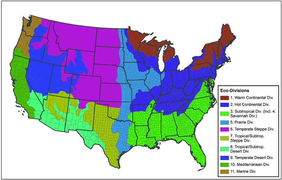
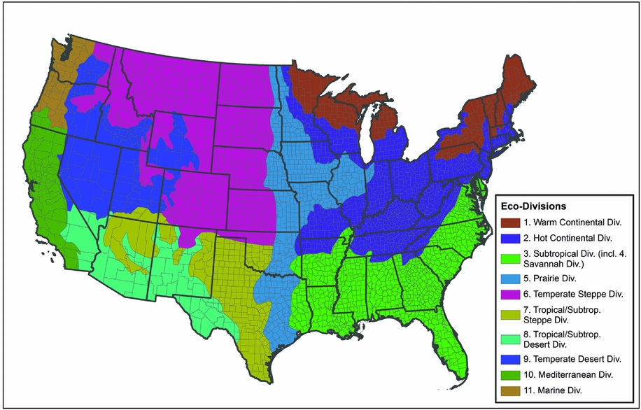
We recognize that there is regional variation in how demographic, economic, agricultural, and environmental characteristics affected the migration patterns of the 1930s. In order to understand this variation, we decided to classify counties into broader groups, using agro-ecological categories defined by the US Forest Service in 1997 (Bailey Reference Bailey1997).Footnote 9 Bailey's report divides the United States into a hierarchical system of ecoregions. These levels of ecoregions include 4 climatic domains, 15 divisions, and 63 provinces. Each of these regional classifications was developed at an increasing level of climatic precision. The division level has the appropriate amount of resolution for our analysis, with 11 divisions for the continental United States, and an additional nine mountain regime subdivisions. To simplify our analysis, we have joined these mountain regimes with their climatic lowland counterpart (i.e., “Subtropical Regime Mountains” is joined with “Subtropical Division”) (see figure 9). We also merged division 4 (Savannah) with division 3 (Subtropical), both of which represent parts of the far southeastern United States, because division 4 only contains four counties at the southern tip of the state of Florida.
Ecodivisions as defined by a United States Forest Service report in 1997.
Along with regional variation, we assume that the dominance of agricultural factors should be less in areas where agriculture plays a smaller role in the economy. One way to do that is to identify urban areas (figure 2). Our starting point for this was a set of historical classifications of metropolitan statistical areas available at the Minnesota Population Center's IPUMS website (“County Composition,” in Ruggles et al. Reference Ruggles, Alexander, Genadek, Goeken, Schroeder and Sobek2010). We created an urban scale variable from the metropolitan area data for 1930. This variable has three values: rural/nonmetro, urban/nonmetro (all nonmetro counties with an urban population greater than 50,000 in 1930), and urban/metro, which are counties classified as metropolitan in 1930, which we further aggregated to two values (rural vs. urban) for our analysis.
Methods
At this stage in our research, most of our data analysis has been descriptive and visual, using maps to show the spatial patterns of migration alongside other spatial patterns—weather, agricultural production and failure, and unemployment. The results, as we will show, are striking, within the usual constraints that it is very difficult to understand correlation or causation visually. What looks like a striking relationship might just be something that catches our eye.
In order to provide a more conventional statistical presentation, we have taken a variety of directions. We begin with ordinary least squares (OLS) regression models with county as the unit of analysis and the natural log of the number of adults (aged 15 or over in 1935) who were resident in the county in 1935 and moved outside the county by 1940 as the dependent variable. All models include the log of the estimated base 1935 population (those who moved plus those who did not) among the explanatory variables. Each model presented explores different combinations of potential explanatory variables. Because there is reason to believe that the relationships of our explanatory variables to our dependent variable vary in different parts of the United States, we also explore the role of ecological divisions in the models. We first consider ecological divisions as a set of binary independent variables. In these OLS models, we find significant heteroskedasticity and a handful of outliers, so we also estimate the models using robust regression methods. While the robust regression models we use might have addressed these issues, in our models it did not do so, as indicated by the Breusch-Pagan p-values in tables 3, 4, and 5.
When residuals from adjacent counties are correlated, that is, spatial autocorrelation, standard OLS estimates of standard errors are artificially small and the goodness of fit measures and chances of finding statistical significance are inflated. Spatial autocorrelation can be measured with Moran's I, and our results show that there is significant spatial autocorrelation in the standard OLS models. It is not possible to calculate Moran's I for the Robust Regression techniques we use, but we suspect that there are spatial effects present.
The third approach we use is to consider ecological divisions as characteristics that interact with all the other variables, and use a method that allows those interactions to uncover how the effects of the other independent variables may depend upon ecological context. Following Anselin (Reference Anselin2007) we refer to the latter as “regime” models because each ecodivision constitutes a separate spatial regime with its own set of regression coefficients. Despite the advantages of the regime models, treating our ecological divisions as different spatial regimes still does not account fully for the spatial effects in the system. This requires a spatial regression approach to reveal the nature and extent of the effects from neighboring counties. Anselin's (Reference Anselin2007) decision tree is the accepted method for choosing between alternative specifications of spatial effects, leading us to choose the “spatial error” model (as opposed to a spatial lag or combined model), because it outperformed other spatial regression and OLS models in our tests. A spatial error model specifies that the unexplained out-migration in a focal county is directly affected by the residual out-migration in the surrounding counties. Regression analyses were largely performed in R, and work that explored patterns in the residuals for different models was conducted in GeoDa (Anselin et al. Reference Anselin, Syabri and Kho2006).
Results
We begin our discussion of results with a visual presentation of adult out-migration by county of residence in 1935 (the results are tabulated by state in table 1). These results are presented in figure 1. These are data where the numerator is the number of people known to live in a specific county in 1935 and who had left by 1940. The denominator for these computations is the sum of all adults (over age 15 in 1935) whose residence was known in 1935 and was within the United States. All individuals living in group quarters in 1940 or living outside the United States in 1935 are excluded.
People who lived in the western United States in 1935 appear more likely to have moved in the next five years than those in the east (and especially New England and the Middle Atlantic states), with the greatest likelihood of out-migration in two north-south bands, one from western Texas and New Mexico north to the Dakotas and Montana (roughly what we consider the Great Plains), and the second away from the coasts in states on the western edge of the United States, especially Arizona, Nevada, California, Idaho, Oregon, and Washington.
What causes these patterns? Certainly, looking back to figure 3.a (temperature in 1934) and figure 4.a (precipitation in 1934), we see possible connections. There is a great deal of out-migration from those places that were hottest and driest in the worst year of the drought. Is this a real relationship? How does it work? Is it a direct connection, or one that works through agriculture? What is the relationship between migration and other factors, such as unemployment, the extent to which the county's population is engaged in farming, or New Deal public programs?
It is possible to quantify the relationships we see with a multivariate statistical analysis. We estimated a series of multivariate OLS models, with various combinations of independent variables. We estimate multivariate models for two families of regressions, one (“Crop Failure”) where the main independent variable is the level of crop failure, and the other (“Climate”), where the main independent variables are precipitation and temperature. We began by estimating univariate regressions between the amount of migration and each of the potential independent variables. For the crop failure model, we achieved stronger associations by dividing the values into four categories (as opposed to a single continuous variable), including 0 percent failure as the reference category. For the climate models, the data for 1934 as a percentage of 1920–40 averages was most predictive of migration. We also include the weighted percent change in production of a county's three top crops as reported in 1930 and 1940 in these models. This measure was more predictive of migration than the other measures, such as the change from 1930 to 1935, or 1935 to 1940, or changes in livestock. In both the crop failure and climate models we include per capita retail and manufacturing employment in 1930, the percent of the working age population unemployed in 1937, and a binary category delineating whether a county is urban (having an urban population in excess of 50,000). For the ecodivisions, we chose the warm continental region in the northeastern United States as the reference category; ecodivisions were added before the other independent variables (except for the log of the total population) when incorporated into models as a main effect.
We hypothesize that there are attributes of counties that encourage or discourage migration, and that these are generally linked to their impact on livelihood. At the core of our analysis are agriculture and the climate forces that shape it, such as drought. We hypothesize that poor agricultural conditions lead to greater out-migration from a county, and that better agricultural conditions are associated with less out-migration. The same holds for unemployment, with greater unemployment associated with higher out-migration. On the other side, we hypothesize that economic activities outside of agriculture will be protective and associated with less out-migration. In that category, we have employment in retail sales and manufacturing, plus the urban status of the county.
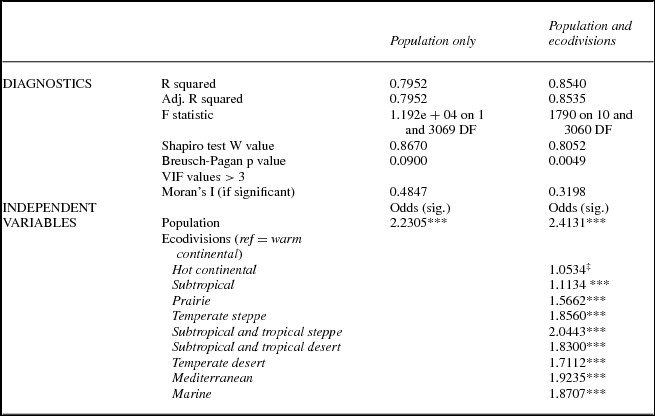
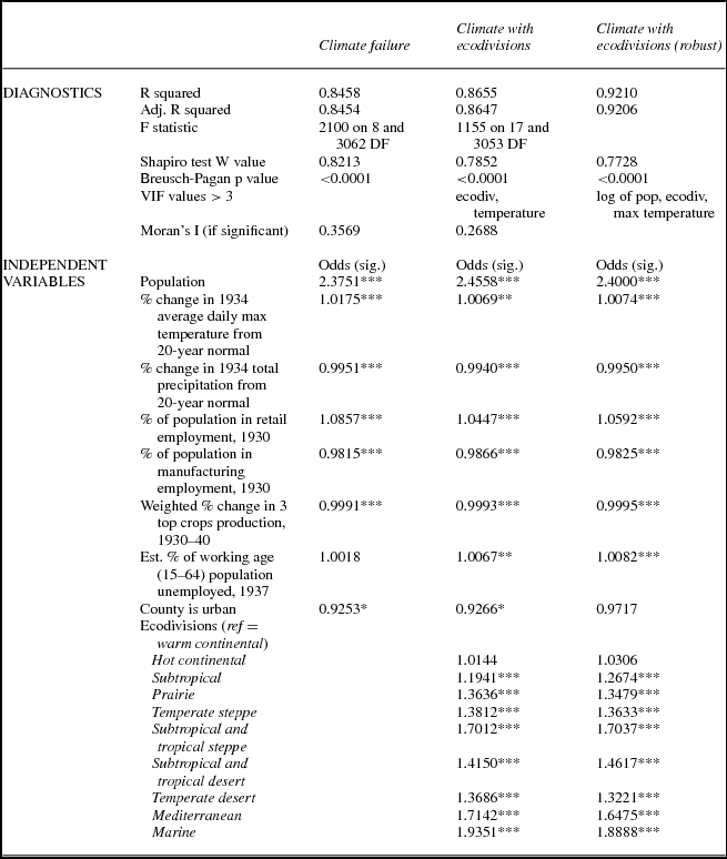
The first and most basic of these results are included in table 2. We begin with a model that just includes the natural log of the baseline population (the denominator in a migration rate) on the right side of the equation. We then add the ecodivisions to the model to show regional effects. All regions (except the Hot Continental division) are significantly different in their level of migration from the Warm Continental reference category. Looking back to figures 3.a and 4.a, we see that the largest coefficients are in areas with the hottest and driest weather in 1934, with the complication that heat and drought did not overlap perfectly—it was hot but not especially dry in the Pacific northwest, and dry but not especially hot in California.
OLS models of county out-migration with population and ecodivisions only

Significance codes: 0: ***; 0.001: **; 0.01: *; 0.05: ‡.
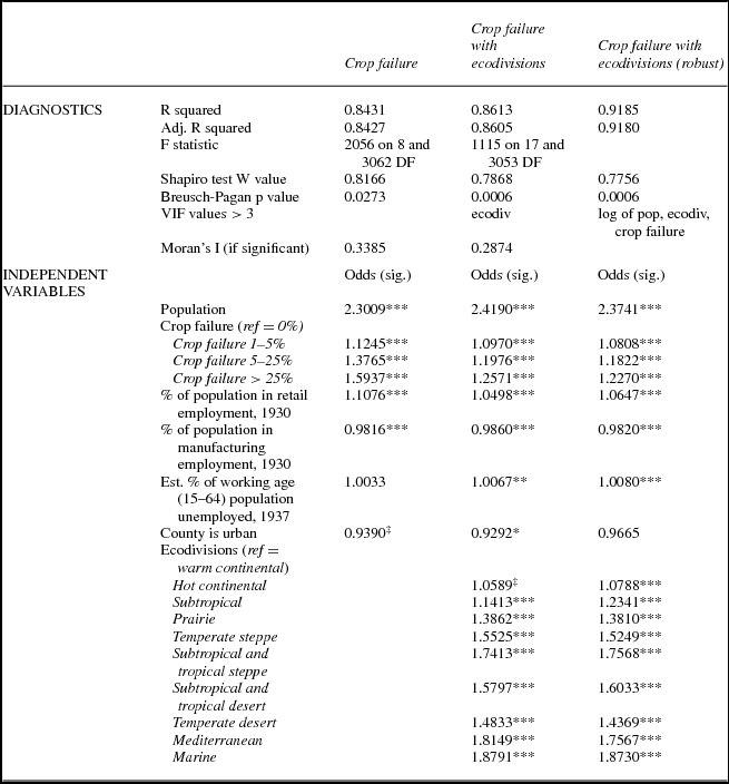
In table 3 we show three versions of a model in which the main independent variable is crop failure, divided into four categories (zero, 1 to 5 percent, 5 to 25 percent, and 25 percent and over). We present two versions of the crop failure OLS model, one with and one without the ecodivisions, as well as a model using robust regression. We present the results as odds ratios. Overall, the OLS model with the ecodivision regions shows a better fit than the one without the ecodivisions, and the robust regression model has an r-squared that is still larger. The results in table 3 largely confirm our assumptions about how environmental and economic stress contributed to migration flows. As expected, higher levels of crop failure led to more migration, as did higher unemployment. By contrast, counties with more manufacturing employment and counties with large urban populations had slightly lower (and not always significantly different) levels of out-migration. The one result that does not necessarily confirm our assumptions is the percent of the population employed in retail, often suggested as an indicator of overall economic activity. Our results show that higher levels of employment in retail sales are associated with higher levels of out-migration from the county, perhaps because of the ubiquity of retail employment throughout the United States in 1930.
OLS models of county out-migration—crop failure models

Significance codes: 0: ***; 0.001: **; 0.01: *; 0.05: ‡.
The US ecodivisions are consistently significant in their impact on out-migration, although there is little difference between the two continental divisions in the northeast and northern Midwest. What the different odds ratios show us is that there was more out-migration in some regions than others (generally in the West), even after we take into account the rest of the model. We will return to this issue later.
In table 4 we replicate the analysis from table 3, with the main independent variables reflecting a combination of climate and agriculture. These variables are precipitation and temperature in 1934 (compared with 1920–40), plus production of the three main crops in the county in 1939, as a percentage of the production of those crops in 1929. These Climate model results confirm what we saw with the Crop Failure models, with a slightly better overall model fit. In these models higher temperatures and lower precipitation, as well as lower agricultural production, are also associated with more out-migration. The other variables generally behave in the same way as they did in the Crop Failure models. One interesting finding is that the unemployment variable only becomes significant when ecodivision is included in the model.
OLS models of county outmigration—climate models
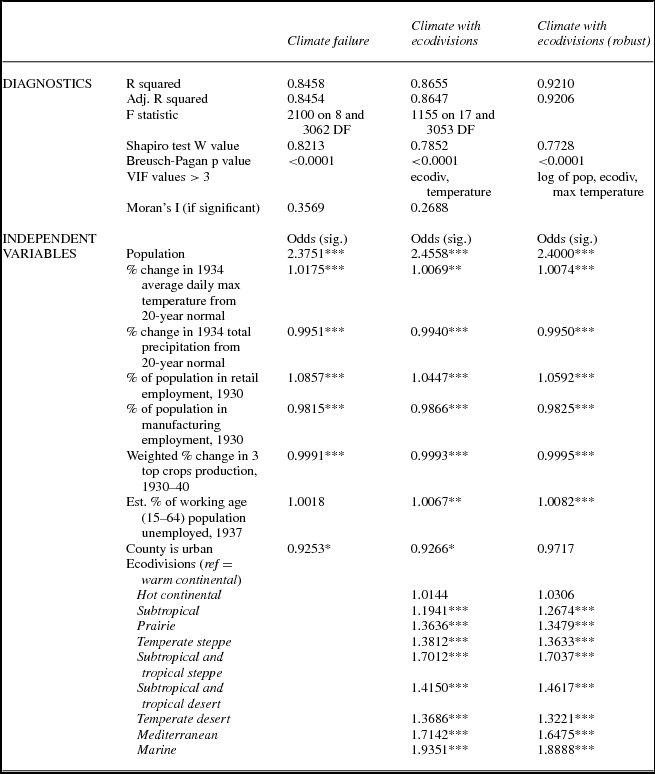
Significance codes: 0: ***; 0.001: **; 0.01: *.
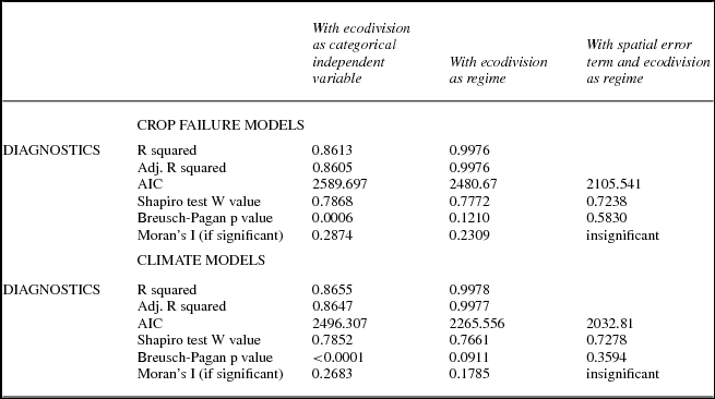
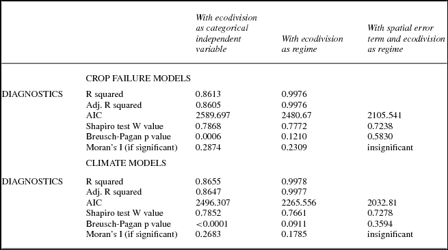
We report the results of our spatial regime models in summary form in table 5, which compares model diagnostics using the ecodivision regions in three ways: as categorical independent variables, a spatial regime model, and a spatial regime model with a spatial error term. Because the spatial regime models involve interactions between the 10 ecodivisions and all the other variables, the coefficients are voluminous. We have chosen not to report them here, but rely in the following text on residual maps to show the spatial characteristics of fit. The diagnostics in table 5 show that by including all of the interactions between ecodivision and the other independent variables we are able to develop a model that explains virtually all of the variance in out-migration, based on an r-squared greater than 0.99. When we then add the spatial error term, improve the fit still further (as indicated by the significantly reduced AIC), and eliminate evidence of spatial autocorrelation (as indicated by an insignificant Moran's I).
Comparison of models using ecodivision with varying techniques
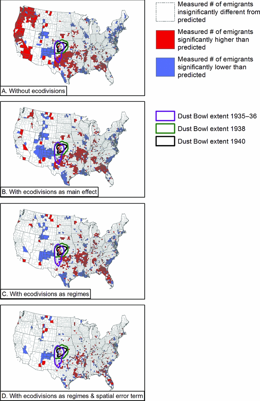
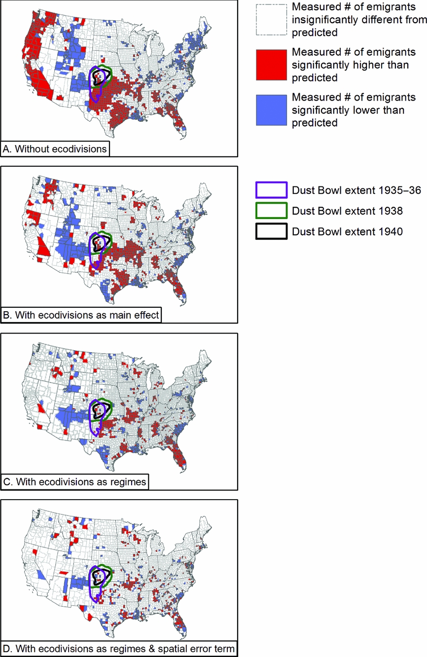
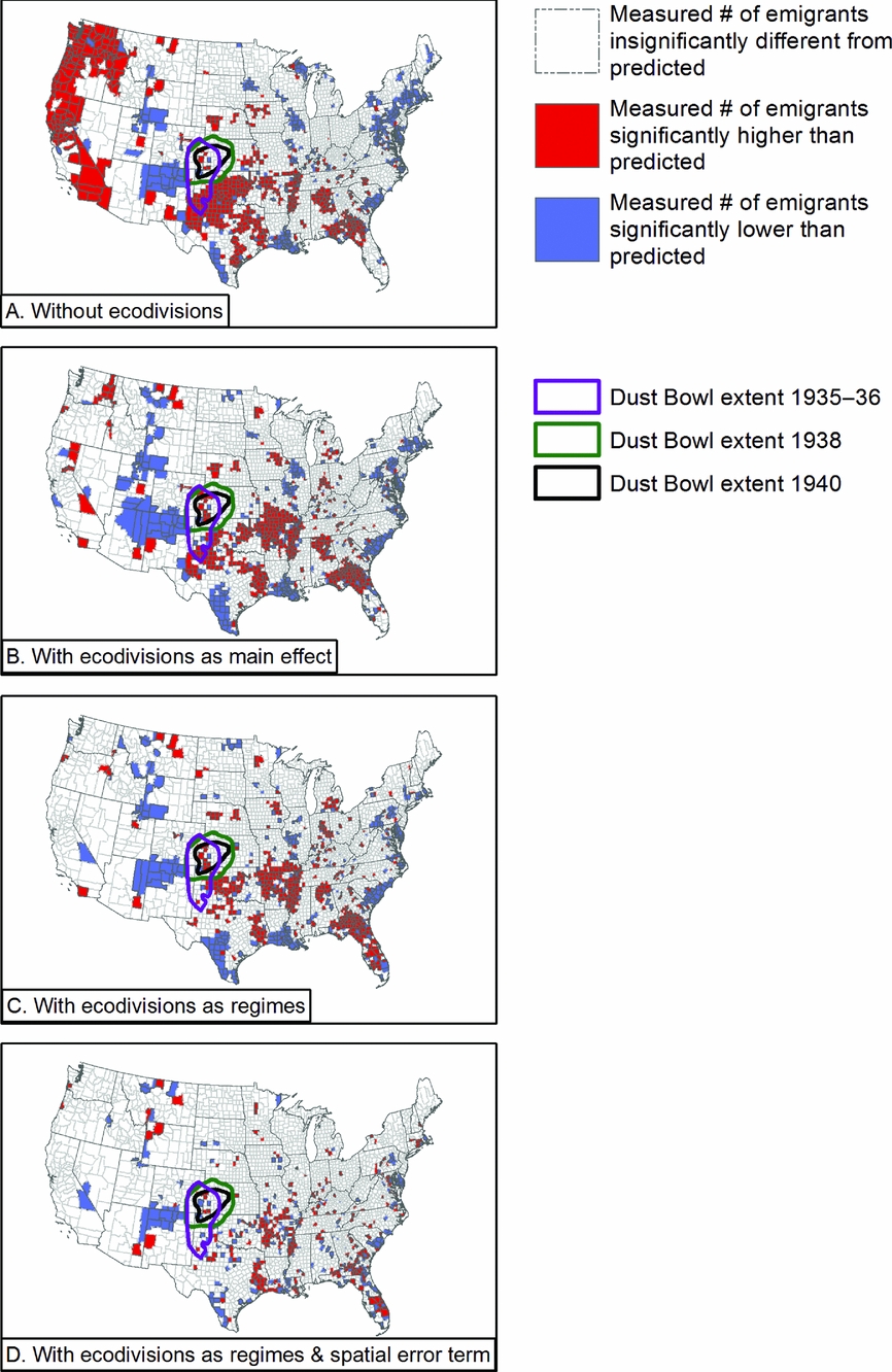
When we introduce the full set of interactions in the regimes model, we achieve a strong model fit, but reveal dramatic heterogeneity among the effects for each combination of independent variable values. We illustrate this heterogeneity in figures 10 and 11 by mapping model residuals. In figure 10 we map the residuals for four versions of our crop failure models, and in figure 11 we do this for the climate models: without ecodivisions, with ecodivisions included as categorical variables, with ecodivisions incorporated as regimes, and with both the ecodivision regimes and a spatial error term to explicitly correct for spatial autocorrelation. We use LISA (local indicators of spatial association) statistics, calculated in GeoDa using contiguity to define neighbor relationships, to better convey the patterns of geographical dependence in our data and our model fits. These four steps allow us to use increasingly effective means for understanding the role of spatial dependence in our data and models. In the maps, white counties are those where the model fits well. Blue counties are areas where the measured migration is significantly lower than predicted by the model, while red counties are ones where the measured migration is significantly higher than predicted by the model.
Mapped residuals of four different implementations of the crop failure model.
Mapped residuals of four different implementations of the climate model.
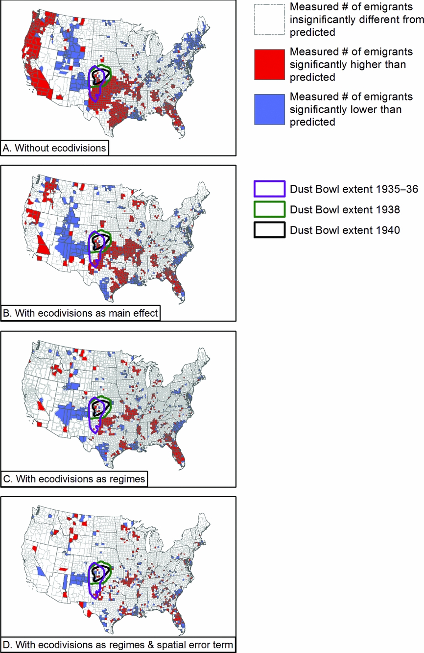
As we progress toward more nuanced appreciations of spatial effects, our overall model fit improves; the number of counties with measured migration significantly different from that predicted by the models (the blue and red counties) decreases. This is a good outcome, confirming the statistical results in table 5, where r-squared, AIC, and other diagnostics improve as we add spatial information. Some areas of poor model fit persist, however. An area in the Southwest remains blue, indicating measured migration is lower than expected and suggesting that an unidentified factor may be providing protection against migration drivers, while red patches scattered across the South indicate that our variables are not accounting for all the drivers of out-migration. These maps also begin to show multicounty patterns that are more localized than what is captured by the ecodivisions. Along the Gulf Coast of Texas, for instance, Harris County, the location of Houston, appears in blue in the final maps, indicating a place of lower than expected out-migration bordered by counties of higher than expected out-migration, perhaps suggestive of an especially strong rural to urban pull due to the rapid growth of the oil industry in Harris County in the 1930s.
The last thing we note in discussing these results is the visual relationship between the residuals and the location of the various periods of dust activity in the 1930s and 1940. In our best models, those areas appear to fit the model relatively well, suggesting that their behavior is well explained by our models, and may not be unusual when compared with other areas of high temperature and low precipitation.
Conclusion
We began this article by asking how much we really knew about the causes of migration in the 1930s. There was a relationship between weather and migration in the 1930s, and it operated beyond the borders of the Dust Bowl. In most of the United States, people left places that were very hot or very dry, and stayed in places that were relatively cool and wet, although that was not true everywhere. Much of the migration-weather process worked through agriculture, but it did not always operate in ways that can be generalized across the whole United States. That is why the models that use temperature and precipitation appear to explain more of the variation in migration than most of the agricultural variables we could find or estimate.
The factors that determine levels of migration during an era of environmental and economic stress are both national and regional in scale. The United States is a large country with strong regional variations in climate, agriculture, and economy, which our analysis reveals. While temperature and precipitation had generalizable impacts on migration in the second half of the Depression, there were noticeable exceptions to the general pattern of how temperature and precipitation related to migration in various parts of the United States. Moreover, while spatial error models captured unobserved spatial processes and reduced the number of counties with unexplained migration outcomes, significant patterns remain. These patterns suggest a wage decline mechanism, rather than an environmental push mechanism, so that people left areas where wages declined. In the Great Plains, heat and drought reduced production, lowering wages and leading to migration. In Georgia, Florida, and along the Mississippi delta, higher production more than production failures drove down wages, which also led to out-migration.
In revealing both national and regional patterns, our work does not discredit the visceral conventional story of 1930s migration that is beautifully illustrated by Steinbeck, or Lange, or described historically by Worster and Gregory; rather, our analysis grounds the drama of what we know about specific cases within a wider context, the nuances of which may only be sketched with the refined and complex data we now have at our disposal. The coexistence of spatially dependent and general processes suggest that future work must continue to explore the nature of multiscalar interactions, and to treat the responses of individual migrants as influenced by places of origin and destination. Even as the work presented here anticipates individual-level analysis, it reminds us that the motivations migrants share, even during an era of widely shared environmental and economic suffering, remain influenced by history and the characteristics of place.
Acknowledgments
This research has been supported by the Institute of Behavioral Science, the Graduate School, the Office of the Vice Chancellor for Research, and the Provost of the University of Colorado. It has benefited from research, administrative, and computing support from the University of Colorado Population Center (CUPC), funded by the Eunice Kennedy Shriver National Institute of Child Health and Human Development (NICHD), Project 2P2CHD066613-06. The content is solely the responsibility of the authors and does not necessarily represent the official views of the CUPC or NICHD. An earlier version of this article was presented at the Annual Meeting of the Social Science History Association in Baltimore, November, 2015. We are grateful for the comments we received at that time, and for the additional comments provided by an anonymous reviewer for Social Science History. Tom Dickinson assisted with data preparation for the environmental variables.
APPENDIX A Deriving Variables about Changes in Agricultural Production for Each County's Three Largest Crops
Using agricultural census data for the years 1930, 1935, and 1940 (which respectively represented farming in 1929, 1934, and 1939) (Haines et al. Reference Haines, Price, Fishback and Rhode2014), we have examined several different types of data as indicators of agricultural production during the period. These data include:
• Percent of total cropland that failed;
• Change in production of major market crops (corn, cotton, and wheat);
• Change in production of major livestock (cattle and pigs). We chose cattle and pigs for our analysis of livestock because these data are most suitable for comparison across census years. The data for other stock animals made comparison more difficult. Work animals such as horses, donkeys, and mules had been in steady decline for some time due to the mechanization of farms; thus, they are not reliable indicators of the health of farms; and
• An agricultural production composite index of the top three crops for each county.
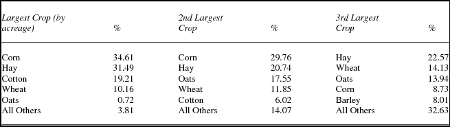
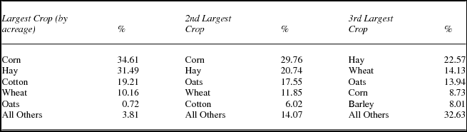
The first three data sets are relatively self-explanatory. The fourth data set, however, requires more explanation. Identifying the most important crops for each of the approximately 3,069 counties in the contiguous United States in our modified data set and then calculating the percent change in production from 1929 to 1939 required several steps. First, we identified the top three crops in each county by the acreage harvested in 1929 (table A.1). The Agricultural Census data for the period contains acreage for nearly all significant crops, meaning any crop that appears in the top three for at least one county. The one major exception is fruit trees: Census takers only recorded the number of trees, rather than the amount of acreage. However, 20 years later, the 1950 Census recorded both acreage and number of trees. This allowed us to estimate the number of acres devoted to fruit trees in each county, assuming that the average number of trees per acre was stable from 1929 to 1949.
Frequency distribution of the top three crops for each county (only five most frequent 1st, 2nd, and 3rd crops are shown)
Second, for each county, we identified the amount of production for each of the top three crops (whether recorded in bushels, bales, pounds, or tons), which we then used to calculate changes in production for the period. The data posed several problems in this effort. Census takers of the period did not record any production values for some crops, most notably vegetables, for which enumerators noted farms reporting, acreage, and dollar values for each vegetable, but not the quantity of production (e.g., bushels). Vegetables were only reported as one of the top three crops in 126 counties, making this gap less problematic. For other crops, the unit of measurement used to record production changed between 1930 and 1940. Most of the time, a simple conversion was sufficient to make the data comparable, an example being that one bushel of cherries weighs approximately 56 pounds, allowing us to convert production in bushels into production in pounds, or vice versa. In a few cases, the data required more complicated conversion calculations. Peanuts are a more complicated example, because they were recorded in bushels in 1930 and 1935, but in pounds in 1940. This posed a problem as different types of peanuts had significantly different rates of pounds/bushel. We worked around this by applying different conversion rates for each state depending on the dominant type of peanut found in that state.
Once we had accounted for all discrepancies in the data, we calculated the percent change in production for each crop across three time periods (1929–34, 1935–39, and 1929–39). In addition, we created a composite index of the percent change of the three crops combined. We created this composite measure by calculating a weighted percent change. For example, in Sutter County, California, barley, wheat, and hay represented 48.8 percent, 40.2 percent, and 11 percent, respectively, of the county's acreage devoted to the top three crops. We multiplied the percent change in production of each crop by the crop's relative size as a weight to create a composite weighted percent change figure.
Appendix B Counties Combined in the Analysis
Appendix C Managing Places of Origin and Matching the Coded and Uncoded Versions of the 1940 Full-count Census
The process of matching the coded and uncoded (raw text) 1940 Census data appears simple, requiring that the data user match on references to the original microfilm reel and manuscript page and line number; all are reported in both data sets. What appears simple turns out to be extremely difficult because IPUMS coding rules (developed for the older sample-based data sets) call for the page number to be “recoded” in order to ensure that all members of a household have the same page number, even when they span multiple pages of the original manuscript. Put another way, when a household spans multiple pages, the page number in the coded data set stays the same, but in the raw text data set page number changes as the page turns. This is a particularly troublesome characteristic if the “household” is an institution (e.g., group quarters, military base, hospital), spanning multiple pages or if intermediate pages are missing. We have developed a script in SAS that corrects the majority of these problems, resulting in a data set that contains 131,438,236 observations (not including Alaska and Hawaii, which have limited other data); the cases lost through our merging process are primarily residents of group quarters, who would be systematically excluded from our analysis in any event. With two exceptions, our data represent between 99 and 101 percent of the official population of each state—and almost 99.9 percent of the official population of the contiguous United States as a whole—as reported in the Historical Statistics of the United States (Carter et al. Reference Carter, Gartner, Haines, Olmstead, Sutch and Wright2006).
Effectively merging the two versions did not produce useable information about the 1935 county of origin of migrants, however. We needed to assign a unique identifier (state and county Federal Information Processing Standard [FIPS] geographical codes) to the 1935 place of residence for everyone enumerated in 1940. For most people, enumerated as being in the “same house” or “same place” and coded as having stayed in their origin county by IPUMS's migrate5 variable, this task was easy: We coded their 1935 county of residence FIPS to the 1940 county of residence FIPS coded by IPUMS. Individuals classified by IPUMS as moving between US counties (21 < migrate5 < 40) were more challenging. We coded the 1935 county of individuals who IPUMS reported as making an intercounty move but who remained within our modified county boundaries (e.g., moves between any of the five counties encompassed by New York City that we have combined into a single “county”) directly from the 1940 county. For individuals who made intercounty or interstate moves by our definition we began by creating a dictionary of unique state and county text strings (from official lists), and used those to assign county IDs for individuals for whom the enumerator had written down a 1935 county of residence. This worked reasonably well, giving us an exact 1935 county of residence for roughly half of all migrants. Two sorts of problems remained: a combination of clerical mistakes by the enumerator and misspelled or incorrectly identified counties, plus respondents reporting only the city of previous residence, and not the county. We resolved this issue by attempting to match the enumerated city-state combination in the uncoded data with a dictionary of unique city-county-state combinations drawn from the coded IPUMS version of the data.
We composed this city-county-state dictionary by extracting all the unique 1940 city-county-state combinations from the coded IPUMS data set using the data set's MIGCITY variable, and removing any entries for cities that spanned more than one county, thus preventing the ambiguous assignment of a county name. Residents with an unknown county but a known city that spanned two or more counties were assigned to the county with the largest area within the city limits (e.g., Amarillo residents with an unknown 1935 county were assigned to Potter County). These changes are shown in Appendix D. Changes made to align the individual-level data with county-level data, described in the following text, also resolved county assignment issues for New York City, St. Louis, and Virginia's independent cities. We have also fixed the miscoding in IPUMS's coded data that coded Richmond County, Virginia, as Richmond City, Virginia.
At the end of these processes, among our population of interest (nongroup quarter adults who remained within the contiguous United States between 1935 and 1940), less than 5 percent had an unknown county of origin.
Appendix D Cities in Multiple Counties