





1 Introduction
Precise prediction of laminar breakdown to turbulence in the boundary-layer flow is indispensable for the design of modern supersonic aircraft, not only due to drag and separation control but also wall heating by friction. With an ever-increasing focus on cutting emissions and increasing the efficiency of the next-generation of supersonic carriers, it has therefore become of vital, topical interest to control the onset of turbulence for high-speed boundary layers.
The oblique-type, first-mode instabilities, breakdown scenario is dominant for the supersonic boundary layer while the acoustic-mode instabilities (Mack modes, Mack (Reference Mack1984)) often dominate in the hypersonic regime. The direct numerical simulation (DNS) studies of Thumm (Reference Thumm1991) and Fasel, Thumm & Bestek (Reference Fasel, Thumm and Bestek1993), for the supersonic boundary layers at Mach number 1.6, were the first ones to report the oblique-type breakdown mechanism. Fezer & Kloker (Reference Fezer and Kloker2000) have investigated the standard oblique-type breakdown with its velocity-streak modes generated by the fundamental unsteady oblique wave pair(s) in combination with subharmonic three-dimensional modes using DNS at Mach 2. They found that the growth rates of three-dimensional subharmonic modes were less significant than those of the fundamental mode and, hence, the standard oblique-type breakdown was found to be dominant. However, the study also concluded that the presence of subharmonic modes did speed-up the transition process. Their findings contradicted the conclusions of Kosinov et al. (Reference Kosinov, Semionov, Shevelkov and Zinin1994) who did not document steady modes at that time. Later on, Mayer, Wernz & Fasel (Reference Mayer, Wernz and Fasel2011) replicated the DNS for the conditions of Kosinov et al. (Reference Kosinov, Semionov, Shevelkov and Zinin1994) and confirmed the importance of oblique-type breakdown mechanism in the experiments. Nowadays it is very clear that the streak modes inherent in oblique breakdown play an essential role as their amplitude grows strongly, fed by nonlinear generation of the unsteady modes and some continuous add-up by a transient-growth mechanism, see Laible & Fasel (Reference Laible and Fasel2016). Streak instability finally causes the laminar breakdown.
Regarding the control of transition in cases where two-dimensional Tollmien–Schlichting waves dominate (incompressible flow), the forcing of control streaks has been investigated, see, for example, Cossu & Brandt (Reference Cossu and Brandt2002), Bagheri & Hanifi (Reference Bagheri and Hanifi2007) or Shahinfar et al. (Reference Shahinfar, Sattarzadeh, Fransson and Talamelli2012). The streak amplitude must not be too high – for otherwise localized shear-layer instabilities cause rapid transition (Andersson et al. Reference Andersson, Brandt, Bottaro and Henningson2001). For oblique breakdown with its inherent streak modes the additional forcing of such modes does not look promising at first, and was only investigated recently in a first study on the interaction of modes by Paredes, Choudhari & Li (Reference Paredes, Choudhari and Li2017). On the other hand, Wassermann & Kloker (Reference Wassermann and Kloker2002) and Saric, Reed & White (Reference Saric, Reed and White2003) successfully investigated the control strategy using appropriate steady control vortex modes for the generic base flow on a swept wing, where cross-flow instability leads to exponential amplification of such steady modes. The findings report that closely spaced vortices can suppress the wider spaced modes responsible for the natural breakdown. Importantly, Wassermann & Kloker (Reference Wassermann and Kloker2002) attributed the suppression of the most-amplified steady modes to the mean-flow distortion (MFD) generated nonlinearly by the control vortices within the upstream flow deformation (UFD) technique. It was found that the two-dimensional (2-D) part of the UFD weakened the growth while the three-dimensional (3-D) part weakened the receptivity of the naturally most-growing modes; for Blasius-flow similar findings concerning the MFD are reported, see, for example, Dörr & Kloker (Reference Dörr and Kloker2017). Stabilization of a supersonic two-dimensional boundary layer using optimally growing streaks has been discussed in the recent study by Paredes et al. (Reference Paredes, Choudhari and Li2017). They utilized the nonlinear plane-marching parabolized stability equations (PSE) to predict the development of finite, stationary disturbances and their interaction with oblique waves. The study concludes that the spanwise wavelength of the control streaks must be smaller than the one of the naturally most-growing oblique travelling modes by a factor of two at least, in order not to reinforce the streak mode inherent in the oblique-breakdown scenario. However, neither DNS nor experiments have so far been reported for the successful control of supersonic boundary-layer oblique breakdown.
Although the PSE study of Paredes et al. (Reference Paredes, Choudhari and Li2017) provides a conceptual model for characterizing a stabilization provided by transiently growing optimal streaks, still some important questions need to be addressed. As later transition stages are completely nonlinear and unsteady, the situation needs a deeper analysis using full DNS. The full effects of ‘control’ streaks, possibly not growing but decaying, are not known for the oblique-type breakdown. How effective are they in the full transition scenario up to turbulence, and which spanwise spacing is useful?
This paper is structured as follows. Section 2 provides the details about the DNS solver used and the boundary conditions, followed by a validation case in § 3. Various aspects about controlling the oblique-type breakdown are presented in § 4; which include the description of the main scenario in § 4.1, the effects of the disturbance spectrum in § 4.2, the effects of control mode amplitude in § 4.3, implications of the spanwise wavenumber of the control mode in § 4.4, the role of the mean-flow distortion and the 3-D part of the control in § 4.5, reinforcing the control mode in § 4.6 and the effect of controlling transition in § 4.7. And finally, the study is concluded in § 5.
2 DNS solver and simulation details
The study utilizes an in-house developed high-order DNS, and large-eddy simulation (LES) code named CHOC-WAVES which solves the three-dimensional, compressible, unsteady Navier–Stokes equations for perfect gases. This code uses a hybrid conservative sixth-order split centred finite-difference scheme with a fifth-order weighted essential non-oscillatory scheme to discretize convective fluxes. Numerical stability is achieved by splitting the convective terms in skew-symmetric form to minimize the aliasing error and to enforce the discrete conservation of the kinetic energy. The diffusive terms are approximated with fourth- or sixth-order schemes and are expressed in Laplacian form. The whole system is time-integrated using a third-order Runge–Kutta scheme. The solver has previously been used for many studies (Shadloo, Hadjadj & Hussain Reference Shadloo, Hadjadj and Hussain2015; Sharma, Shadloo & Hadjadj Reference Sharma, Shadloo and Hadjadj2018a ,Reference Sharma, Shadloo and Hadjadj b ). The validation case for the current study is presented in § 3.
2.1 Simulation set-up
A supersonic boundary layer with free-stream Mach number
 $M_{\infty }=2.0$
is investigated using DNS. The fluid is supposed to be a perfect gas with constant specific heats. The set-up is designed to keep the flow conditions of Fezer & Kloker (Reference Fezer and Kloker2000) or Mayer et al. (Reference Mayer, Wernz and Fasel2011). The free-stream temperature is
 $T_{\infty }^{\ast }=160$
K, velocity
 $u_{\infty }^{\ast }=507.1~\text{m}~\text{s}^{-1}$
, viscosity
 $\unicode[STIX]{x1D708}^{\ast }=2.1067\times 10^{-5}~\text{m}^{2}~\text{s}^{-1}$
, pressure
 $p_{\infty }^{\ast }=23.786$
kPa and Prandtl number
 $Pr=0.72$
. The flow domain is free of any shocks generated from the leading edge of the plate because the inlet of the domain is kept downstream of the leading edge at
 $x_{in}^{\ast }=0.004154$
m with inlet Reynolds number
 $Re_{x_{in}}=10^{5}$
and unit Reynolds number
 $Re_{u}^{\ast }=2.407\times 10^{7}~\text{m}^{-1}$
. The boundary-layer thickness at the inlet is
 $\unicode[STIX]{x1D6FF}_{in}^{\ast }=7.958\times 10^{-5}$
m. The length and height of the domain are
 $L_{x}^{\ast }=0.055$
m (
 $L_{x}/\unicode[STIX]{x1D6FF}_{in}=691.13$
) and
 $L_{y}^{\ast }=0.0102$
m (
 $L_{y}/\unicode[STIX]{x1D6FF}_{in}=128.17$
), respectively. The width of the domain corresponds to the fundamental wavelength
 $L_{z}^{\ast }=\unicode[STIX]{x1D706}_{z}^{\ast }=0.002153$
m (
 $L_{z}/\unicode[STIX]{x1D6FF}_{in}=27.05$
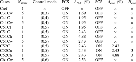
) of the disturbed mode. But for the validation case, a four times broader domain was chosen to include the subharmonic modes considered by Fezer & Kloker (Reference Fezer and Kloker2000). Table 1 lists the various cases investigated in this study. Equidistant grid spacing is utilized in streamwise (
 $x$
) and spanwise (
 $z$
) directions with
 $N_{x}=800$
and
 $N_{z}=140$
points, respectively. Grid stretching is used in wall-normal direction, defined as
 $$\begin{eqnarray}y=L_{y}^{\ast }\left(1+\frac{\tanh \unicode[STIX]{x1D705}y}{\tanh \unicode[STIX]{x1D705}}\right),\end{eqnarray}$$
where,
 $\unicode[STIX]{x1D705}=3$
is the grid stretching parameter. The number of points in wall-normal (
 $y$
) direction are
 $N_{y}=180$
.
Simulation parameters for various cases.
 $N_{modes}$
, FCS, SCS,
 $A_{FCS,SCS}$
and
 $H_{SCS}$
stand for the number of modes excited, first control strip, second control strip, the amplitudes at the first and the second control strip (
 $A_{FCS,SCS}=(\unicode[STIX]{x1D70C}v)_{w,max}/\unicode[STIX]{x1D70C}_{\infty }u_{\infty }$
), and the number of harmonics used in the second control strip, respectively. Suffix
 $h$
,
 $l$
,
 $n$
and
 $w$
represent cases with high, low intensity of the control mode, narrow crests of SCS and wide disturbance spectrum, respectively.
2.2 Boundary conditions
At the inlet of the domain, physical quantities like streamwise and wall-normal velocity, and density profiles obtained from the similarity solution of a laminar compressible adiabatic boundary layer are specified. Supersonic inflow and outflow conditions are chosen at the inlet and outlet of the domain at
 $x_{in}^{\ast }$
and
 $x_{out}^{\ast }=x_{in}^{\ast }+L_{x}^{\ast }$
, respectively. Periodic boundary conditions are used for the side-walls of the domain. The no-slip and no-penetration condition is used at the surface of the wall except for the blowing–suction and control strips which are used to excite the test-modes and introduce the stabilization streaks, respectively, in the domain. The temperature at the wall is calculated by considering the adiabatic zero-gradient condition everywhere, and for the top surface a slip condition with zero boundary-normal gradient is imposed.
2.2.1 Blowing and suction
The laminar boundary layer is perturbed using blowing and suction which introduces an excitation in
 $(\unicode[STIX]{x1D70C}v)_{wall}/\unicode[STIX]{x1D70C}_{\infty }u_{\infty }$
. This strip extends from
 $x_{1}^{\ast }=(x_{in}^{\ast }+0.004154)$
m to
 $x_{2}^{\ast }=(x_{in}^{\ast }+0.009654)$
m, and can be expressed as
 $$\begin{eqnarray}\displaystyle & \unicode[STIX]{x1D70C}v(x,y=0,z,t)=A\unicode[STIX]{x1D70C}_{\infty }u_{\infty }\,f(x)g(z)h_{1}(t), & \displaystyle\end{eqnarray}$$
 $$\begin{eqnarray}\displaystyle & f(x)=4\sin \unicode[STIX]{x1D703}(1-\cos \unicode[STIX]{x1D703})/\sqrt{27}, & \displaystyle\end{eqnarray}$$
 $$\begin{eqnarray}\displaystyle & \unicode[STIX]{x1D703}=2\unicode[STIX]{x03C0}(x-(x_{1}^{\ast }-x_{in}^{\ast }))/(x_{2}^{\ast }-x_{1}^{\ast }), & \displaystyle\end{eqnarray}$$
 $$\begin{eqnarray}\displaystyle & \displaystyle g(z)=(-1)^{k}\cos \left(\frac{2\unicode[STIX]{x03C0}kz}{L_{z}^{\ast }}\right), & \displaystyle\end{eqnarray}$$
 $$\begin{eqnarray}\displaystyle & h_{1}(t)=\sin (h\unicode[STIX]{x1D714}t), & \displaystyle\end{eqnarray}$$
where
 $A$
is the disturbance amplitude given as
 $(\unicode[STIX]{x1D70C}v)_{wall}/(\unicode[STIX]{x1D70C}_{\infty }u_{\infty })$
,
 $\unicode[STIX]{x1D714}$
is the angular frequency of the excitation mode,
 $h$
is the multiple of the fundamental frequency and
 $k$
is the multiple of the fundamental spanwise wavenumber. The expressions for
 $f(x),\unicode[STIX]{x1D703}$
and
 $h_{1}(t)$
are taken from Pirozzoli, Grasso & Gatski (Reference Pirozzoli, Grasso and Gatski2004). For all the cases listed in table 1,
 $A=6.5\times 10^{-4}$
. The fundamental frequency
 $f_{0}^{\ast }=73.83$
kHz and wavenumber
 $\unicode[STIX]{x1D6FD}_{0}^{\ast }=2\unicode[STIX]{x03C0}/\unicode[STIX]{x1D706}_{z}^{\ast }=2.9176\times 10^{3}~\text{m}^{-1}$
, which correspond to their dimensionless counterparts used by Fezer & Kloker (Reference Fezer and Kloker2000), are excited in this study, i.e. modes (1,1) and (1,
 $-1$
), designating the frequency/spanwise wavenumber tuple. Here, (
 $h$
,
 $k$
) denotes the mode with frequency
 $hf_{0}^{\ast }$
and spanwise wavenumber
 $k\unicode[STIX]{x1D6FD}_{0}^{\ast }$
. In the following, (
 $h$
,
 $k$
) stands for the sum of (
 $h$
,
 $+k$
) and (
 $h$
,
 $-k$
). Various (
 $h$
,
 $k$
) modes are excited for Cx1Cw cases (details in § 4.2).
2.2.2 Control streak strips
Control streaks are introduced using additional strips to control the transition process. Their formulation is quite similar to that of the unsteady blowing–suction but these perturbations are steady and the function in
 $x$
is altered. Note that no net mass flux is introduced because there is no 2-D part in the wall-function. For all the cases mentioning
 $FCS$
‘ON’ in table 1, this strip runs from
 $x_{c_{1.1}}^{\ast }=(x_{in}^{\ast }+0.002)$
m to
 $x_{c_{1.2}}^{\ast }=(x_{in}^{\ast }+0.004)$
m,
 $$\begin{eqnarray}\displaystyle & \unicode[STIX]{x1D70C}v(x,y=0,z)=A_{FCS}\unicode[STIX]{x1D70C}_{\infty }u_{\infty }\,f(x)g(z), & \displaystyle\end{eqnarray}$$
 $$\begin{eqnarray}\displaystyle & f(x)=2.5983(1-\cos \unicode[STIX]{x1D703})/\sqrt{27} & \displaystyle\end{eqnarray}$$
here,
 $\unicode[STIX]{x1D703}$
and
 $g(z)$
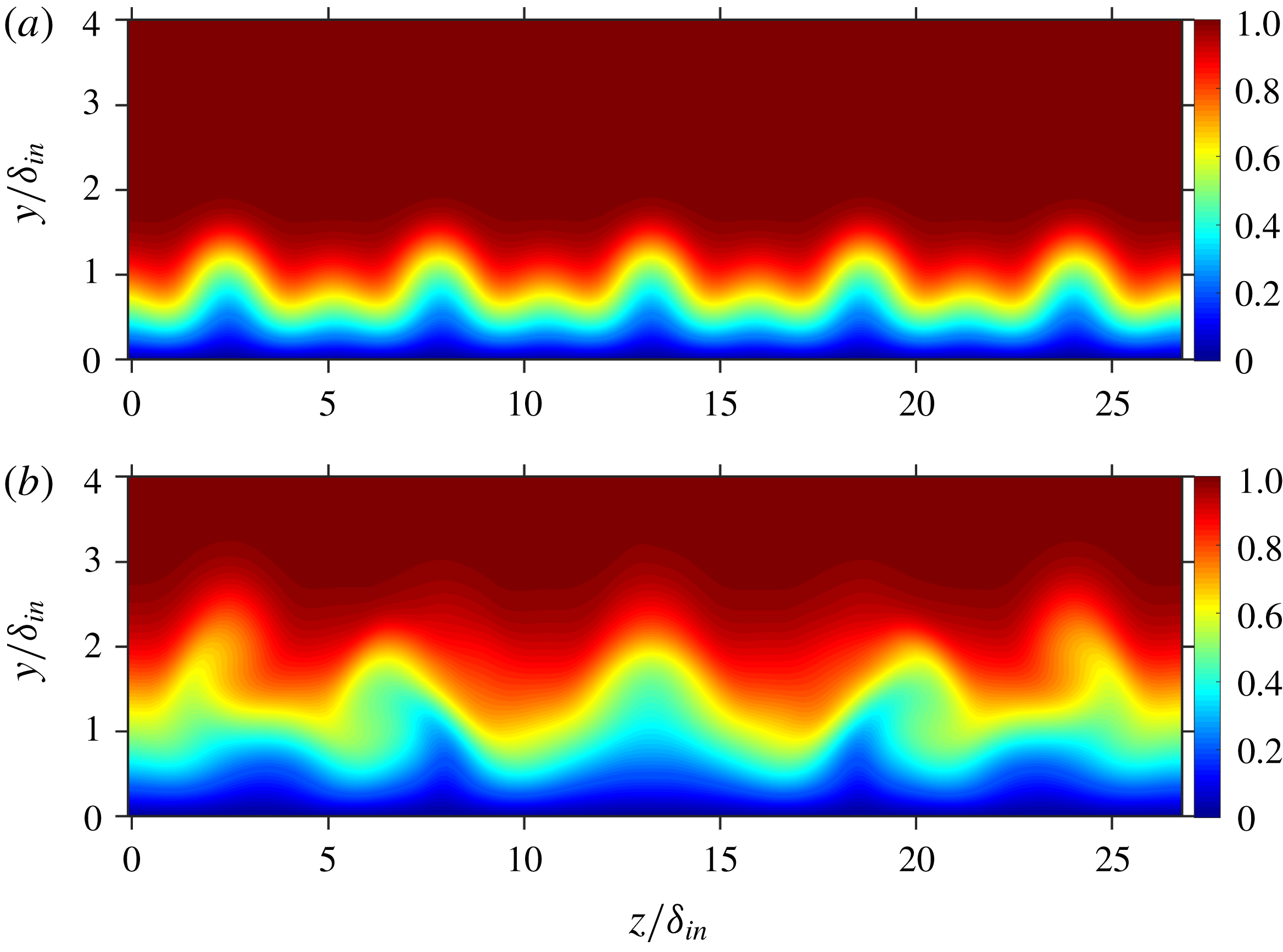
have same formulations as defined earlier in § 2.2.1, see figure 13(a). Additionally, for cases with
 $SCS$
‘ON’, another more downstream control strip is used which extends from
 $x_{c_{2.1}}^{\ast }=(x_{in}^{\ast }+0.01664)$
m to
 $x_{c_{2.2}}^{\ast }=(x_{in}^{\ast }+0.01864)$
m. For cases C52Cn and C52Ch a different formulation of
 $g(z)$
has been used (details will be described in § 4.6), which is given as
 $$\begin{eqnarray}g(z)=\frac{1}{3}\times \left[-\text{cos}\left(\frac{2\unicode[STIX]{x03C0}\times 5z}{L_{z}^{\ast }}\right)+\cos \left(\frac{2\unicode[STIX]{x03C0}\times 10z}{L_{z}^{\ast }}\right)-\cos \left(\frac{2\unicode[STIX]{x03C0}\times 15z}{L_{z}^{\ast }}\right)\right].\end{eqnarray}$$
3 Validation
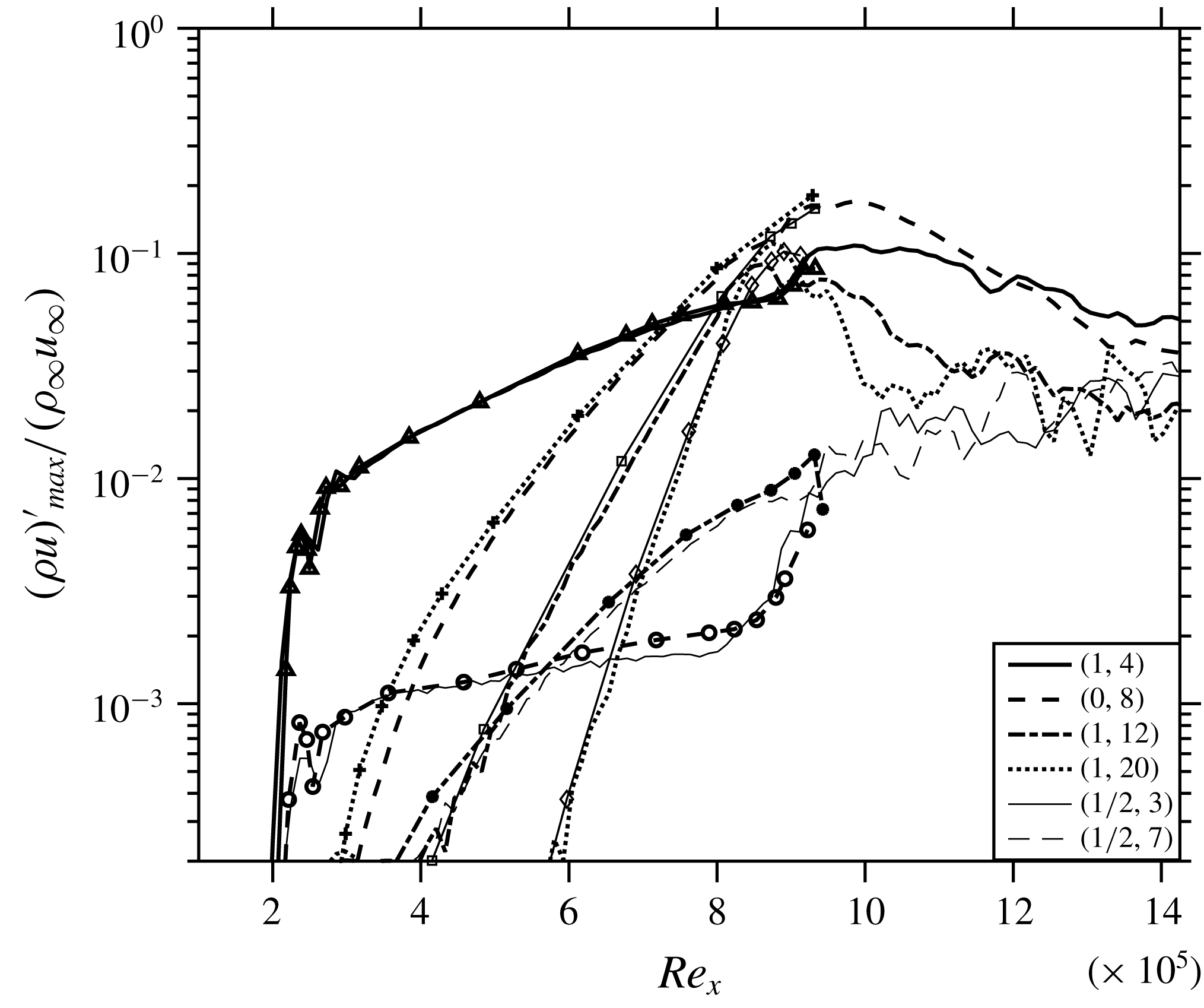
In order to validate the solver for growth rates of various modes in the boundary layer, ‘Case 1’ computed by Fezer & Kloker (Reference Fezer and Kloker2000), see also Mayer et al. (Reference Mayer, Wernz and Fasel2011), is taken as the reference benchmark. See the latter paper also for an overview of the stability characteristics of the flow as obtained by linear stability theory. Modes (1,4) and (
 $1/2$
,3) are excited using blowing–suction. It should be noted here that the details of blowing and suction used by Fezer & Kloker (Reference Fezer and Kloker2000) are not provided in their study, therefore the amplitudes of the fundamental and subharmonic modes are adjusted to match with the respective initial amplitudes. Figure 1 compares various modes of the current DNS with their counterparts by Fezer & Kloker (Reference Fezer and Kloker2000), marked by symbols. The curves show a good collapse assuring that the DNS correctly predicts the growth of various modes. Each mode is computed by time-sampling over two fundamental periods, then performing a Fourier transform in the spanwise direction followed by one with respect to time, and then obtaining the maximum value in wall-normal direction at a given streamwise station. In order to cut the computational cost, a quarter of the domain used for validation is considered in the reference case Cref for the remainder of the study. No subharmonic excitation is employed, only the fundamental mode (1,1), which peaks in growth rate in the frequency-spanwise wavenumber spectrum, is excited. Moreover, Cref is seven times more refined in the spanwise direction than the original case used for validation. The instantaneous flow-field for Cref is shown in figure 4(a) which prominently displays the oblique-type breakdown close to
 $Re_{x}=9\times 10^{5}$
.
Comparison of the streamwise evolution of the maximum disturbance amplitudes of various modes with Fezer & Kloker (Reference Fezer and Kloker2000) (marked by symbols).
4 Controlling transition
4.1 Main scenario
In an attempt to control the transition to turbulence, control mode (0,5) – as a result of various trials, see below – is utilized, which is forced using a control strip running from
 $Re_{x}=1.48\times 10^{5}$
to
 $Re_{x}=1.96\times 10^{5}$
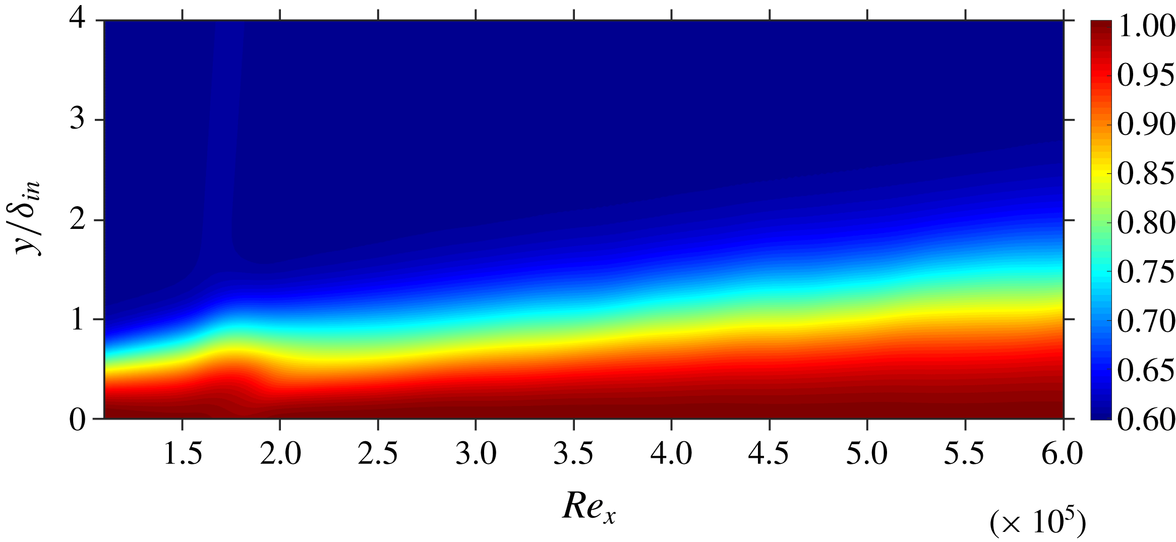
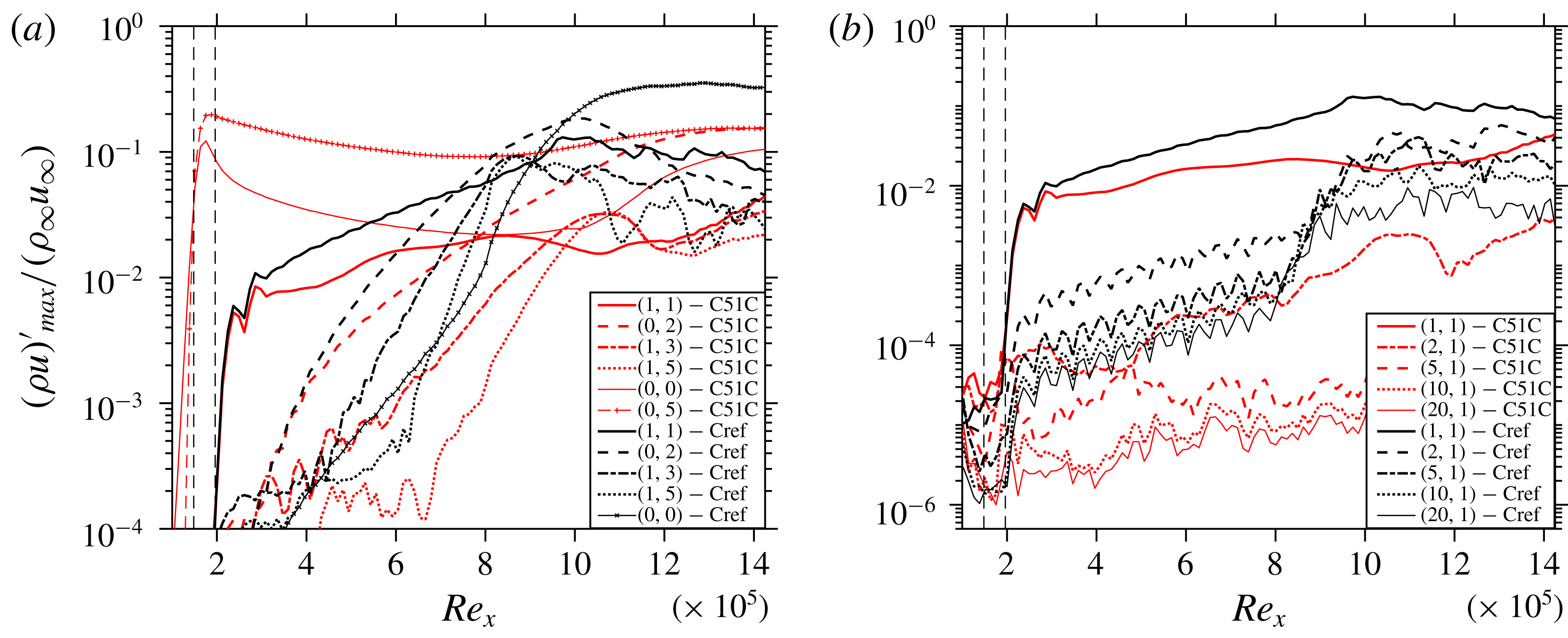
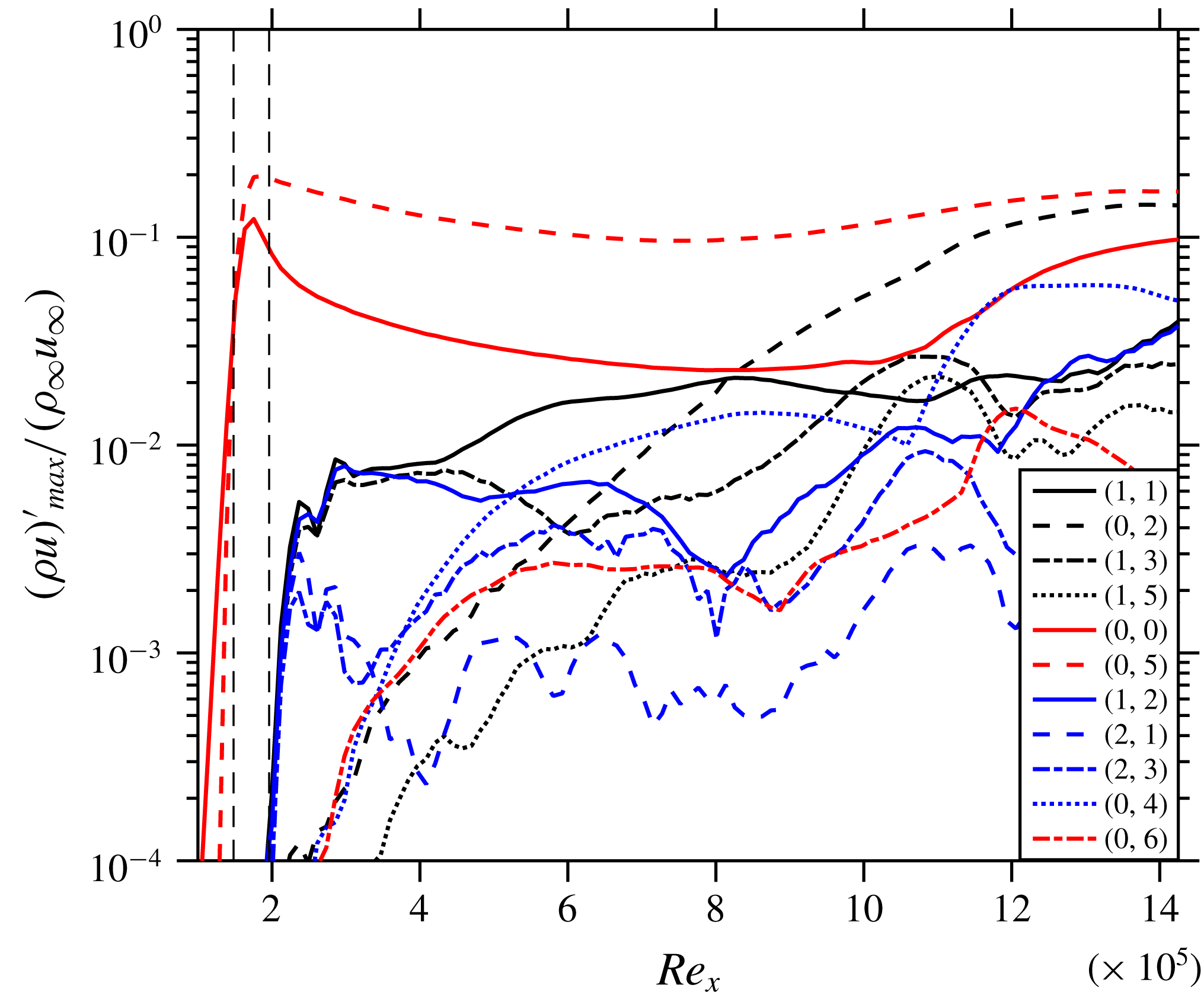
(case C51C). The longitudinal cut for C51C, coloured by the contours of temperature shown in figure 2, clarifies that no local temperature jump is introduced due to the induction of the steady control streak mode. The induced control mode indeed successfully suppresses the transition. It can be seen in figure 3(a) that, as a result of introduction of the control streak mode (location marked by vertical dashed lines) (0,5), a large MFD (0,0) is generated (
 ${\approx}12\,\%$
of
 $\unicode[STIX]{x1D70C}_{\infty }u_{\infty }$
), and the control modes lead to the reduction of the growth rates of the main 3-D modes (1,1) and (0,2) in comparison to Cref. The MFD is a part of the stabilization of the flow, as will be shown below in § 4.5. The evolution of high-frequency modes initiated by the numerical background noise shown in figure 3(b) depicts significant suppression for C51C. This difference is as large as three orders of magnitude towards the end of the domain because of the missing breakdown with control. The initial noise level generated from the solver is
 ${\approx}10^{-5}$
of
 $\unicode[STIX]{x1D70C}_{\infty }u_{\infty }$
(see figure 3
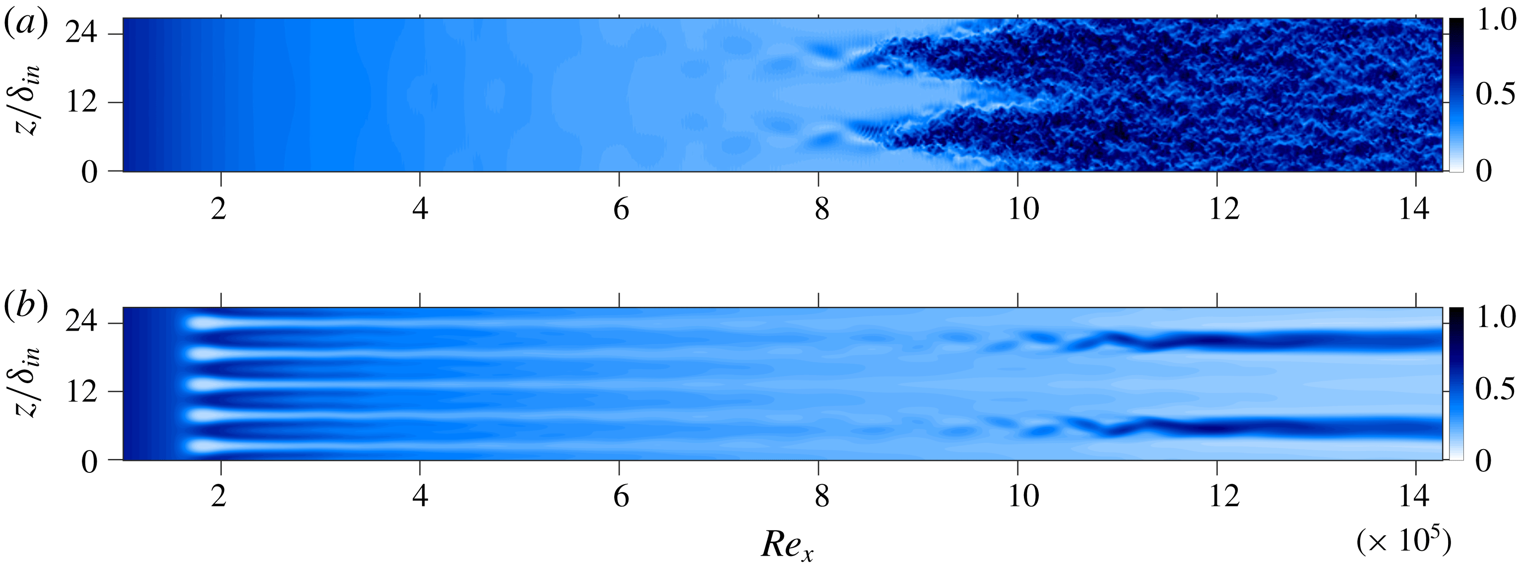
b). Figure 4(b) shows the instantaneous flow-field for C51C demonstrating complete suppression of the turbulent region. Towards the end of the domain, (0,2) high-speed streaks can be prominently seen as a result of their higher amplitude from
 $Re_{x}=10^{6}$
onwards (see figure 3
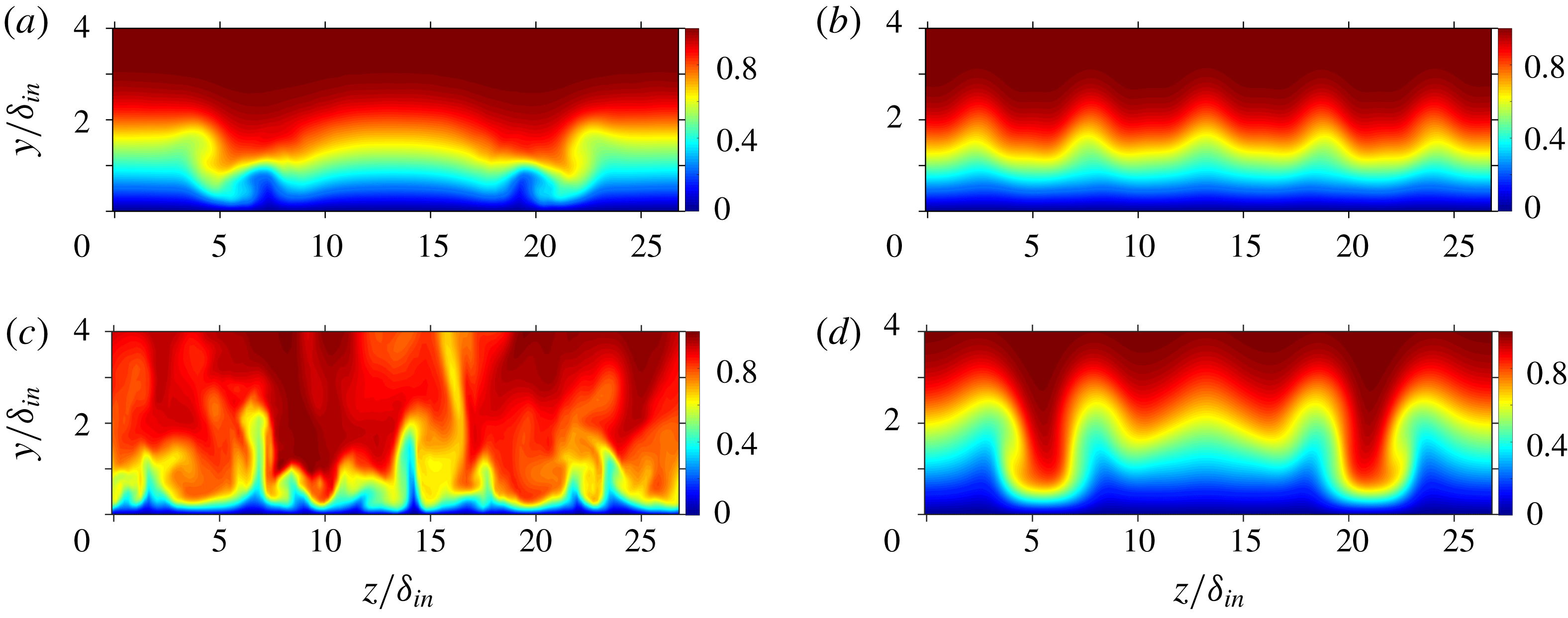
a). It is to be noted that no streak instability sets in despite the large (0,2) amplitude that however is enriched by the (0,5) control mode and (0,0). Flow cross-cuts in figure 5 show the early stage of transition of Cref in figure 5(a) while C51C remains stable at this location (see figure 5
b) due to less pronounced low-speed regions. A comparison of figures 5(c) and 5(d) reveals a more stable nature of the streaky boundary layer of C51C compared to Cref due to the existence of the two high-speed streaks intruding into the low-speed near-wall region and preventing the build-up of strong, unstable low-speed regions, cf. figures 5(a) and 5(c).
Longitudinal cut for C51C: contours of
 $T/T_{w}$
at
 $z/\unicode[STIX]{x1D6FF}_{in}=13.5$
.
Comparison of the streamwise evolution of the maximum (a) disturbance amplitudes of various modes, and (b) amplitudes of high-frequency modes: C51C versus Cref.
Instantaneous flow-fields for (a) Cref, and (b) C51C: contours of
 $u/u_{\infty }$
, shown at
 $y/\unicode[STIX]{x1D6FF}_{in}=0.48$
.
Contours of
 $u/u_{\infty }$
for (a,b) at
 $Re_{x}=8.6\times 10^{5}$
, (c) (snapshot) and (d) at
 $Re_{x}=13\times 10^{5}$
, (a,c) case Cref, (b,d) C51C.
4.2 Larger disturbance spectrum
The results presented so far prove the effectiveness of the considered control mode (0,5) in controlling the oblique-type breakdown induced by the fundamental symmetric mode (1,1). To investigate the effect of a broader disturbance input we consider the case C51Cw comprising of a total of five disturbance modes which are forced simultaneously in the same blowing–suction strip, each having the same amplitude as the fundamental mode before. The additional modes are (1,2), (1,3), (2,1), (2,3), to include higher spanwise wavenumbers being closer to the control-mode wavenumber and to provide modes that fill the gaps directly or by the nonlinear interaction that exists in the pure, fundamental case with (1,1) only. Likewise C51C, the transition is successfully suppressed in C51Cw despite the larger total forcing amplitude, see figure 6. It can be seen that (2,1) and (2,3) do not alter the scenario palpably. Modes (1,2) and (1,3) nonlinearly generate the streak modes (0,4) and (0,6), respectively, which are much closer to the spanwise wavenumber of the control mode (0,5), than the (0,2) of the fundamental mode. This may compromise the control strategy according to intuition and the findings of Paredes et al. (Reference Paredes, Choudhari and Li2017). However, it can be seen from figure 6 that the control mode (0,5), with the applied amplitude and the generated MFD (0,0), still successfully suppresses the significant growth of the relevant 3-D modes.
Streamwise evolution of the maximum disturbance amplitudes of various modes for C51Cw.
4.3 Effects of control-mode amplitude
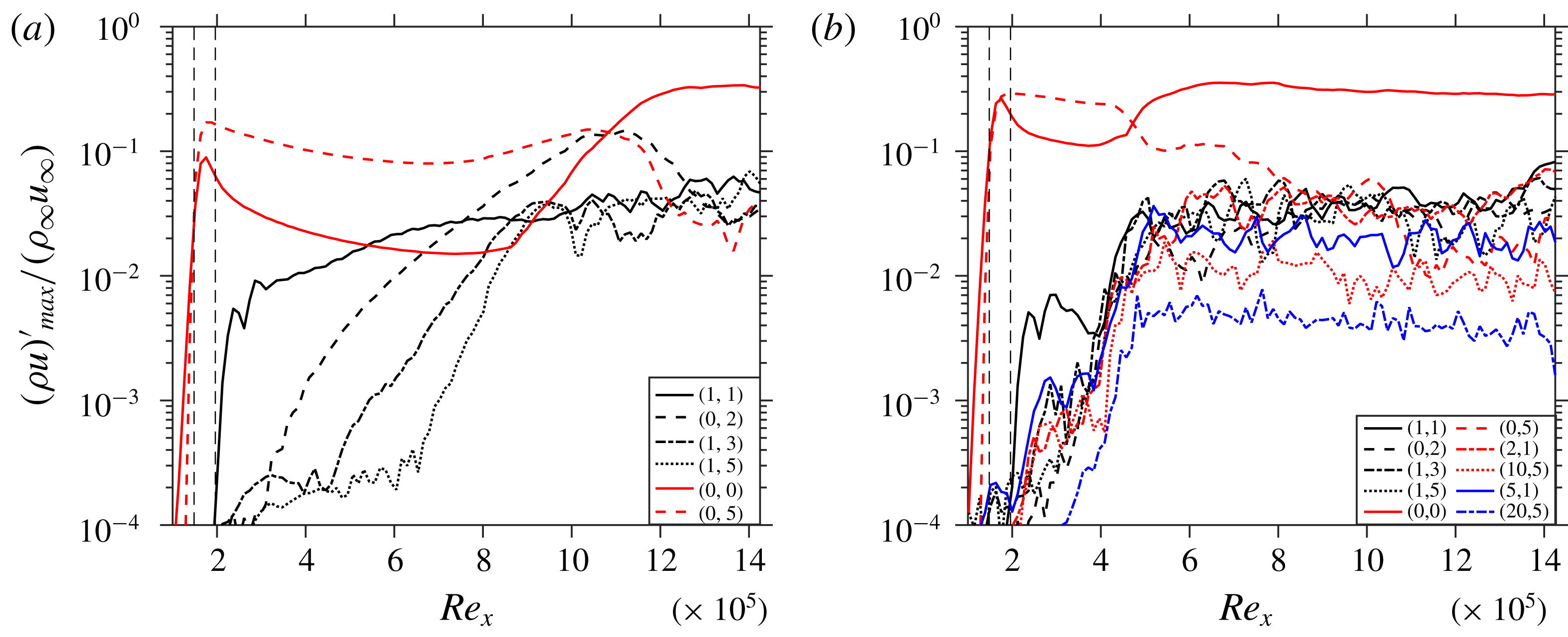
The two cases C51Cl and C51Ch with lower and higher forcing amplitudes of the control mode, respectively, are compared to C51C. Figure 7(a) shows the evolution of various modes for C51Cl; the sudden shoot-up of (0,0) close to
 $Re_{x}=8\times 10^{5}$
signifies transition to turbulence. It can be implied from this figure that because of both the lower forcing amplitude of the control mode (0,5) and the MFD (
 ${\approx}9\,\%$
of
 $\unicode[STIX]{x1D70C}_{\infty }u_{\infty }$
) transition cannot be suppressed. On the other hand, the high forcing amplitude of the control mode (0,5) in case C51Ch (figure 7
b) causes rapid transition close to
 $Re_{x}=5\times 10^{5}$
, see figure 8, as a result of strong streak-mode instability. The control-effective amplitude window is thus expectedly limited. Streaks with a modal
 $\unicode[STIX]{x1D70C}u$
amplitude larger than about 25 % cause localized high-frequency instability even if they are closely spaced, as here.
Streamwise evolution of the maximum disturbance amplitudes of various modes for cases (a) C51Cl, and (b) C51Ch.
Instantaneous flow-field for C51Ch: contours of
 $u/u_{\infty }$
, shown at
 $y/\unicode[STIX]{x1D6FF}_{in}=0.48$
.

4.4 Implications of spanwise wavenumber of control mode
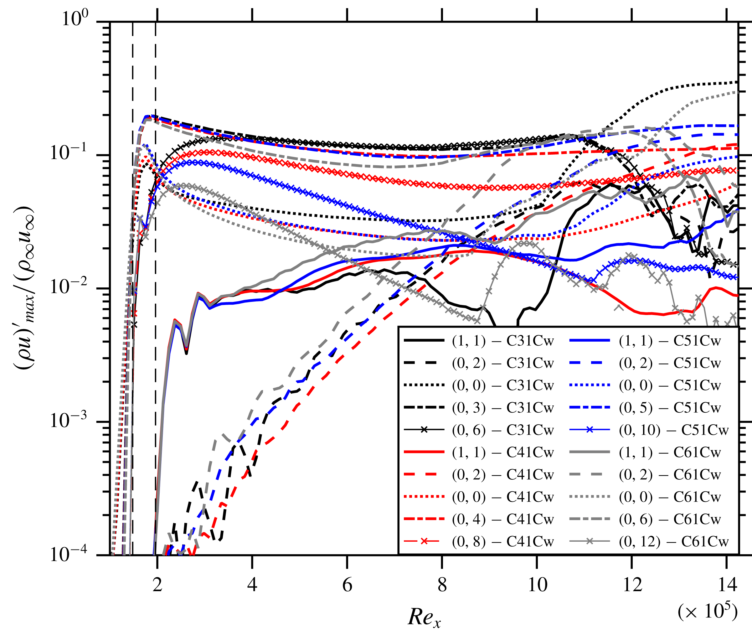
The effect of the spanwise wavenumber is investigated using four cases: C31Cw, C41Cw, C51Cw and C61Cw, employing control modes (0,3), (0,4), (0,5) and (0,6), respectively, with the wide disturbance spectrum. These control modes are induced with different forcing amplitudes (see table 1) in order to have the same effective Fourier amplitude at the end of the control strip (see figure 9). This comparison plot reveals that the streaks and generated MFD (0,0) decay is stronger the higher the spanwise wavenumber of the control mode is, except for C41Cw and C51Cw that behave similarly. On comparing the (0,0) modes further downstream it becomes clear that C31Cw and C61Cw do not show working control because their (0,0) modes shoot-up suddenly at
 $Re_{x}=10\times 10^{5}$
and
 $Re_{x}=9\times 10^{5}$
, respectively, signifying transition. C61Cw generates the lowest of all control MFDs, and as soon as it falls below about 2 % of
 $\unicode[STIX]{x1D70C}_{\infty }u_{\infty }$
, the flow shows early signs of transition at about
 $Re_{x}=8\times 10^{5}$
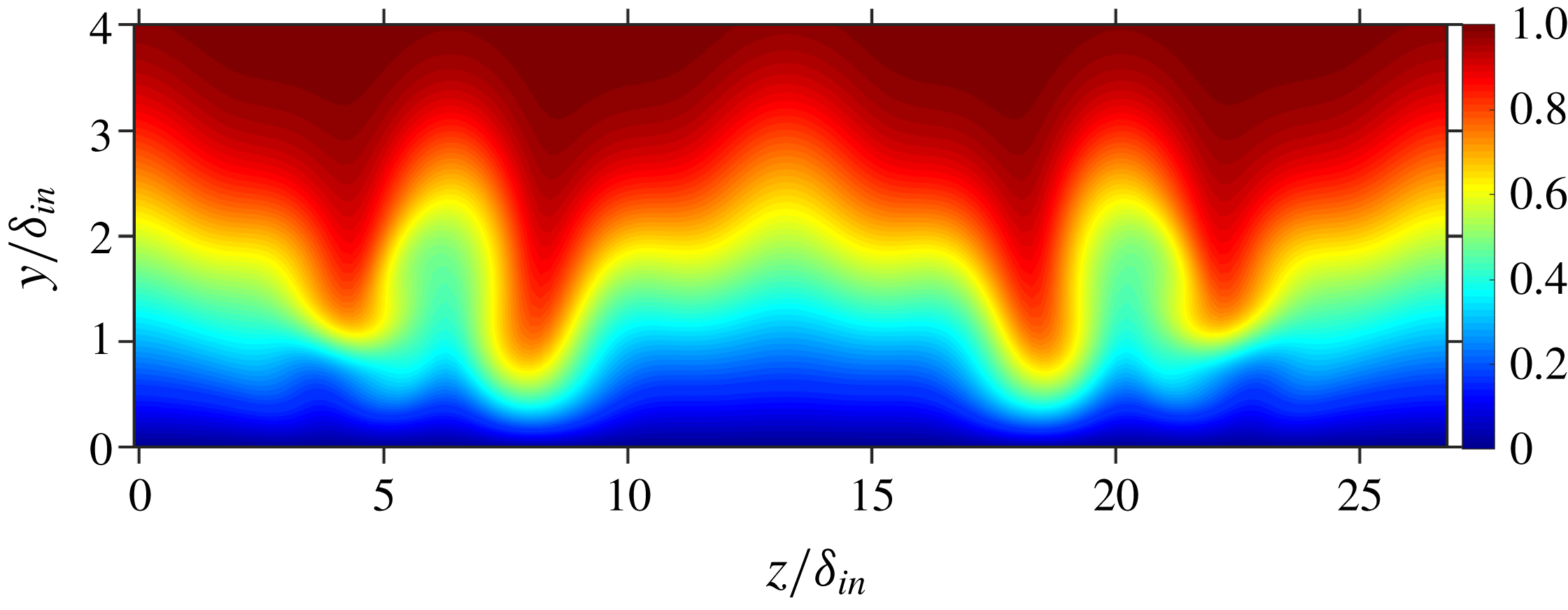
. Hence, the growth rate of (1,1) is strongest for C61Cw. As a result of the high forcing amplitude of the control modes, relevant modes with double spanwise wavenumber are generated nonlinearly. The interaction of the generated (0,6) by control mode (0,3), which is as strong as the (0,3) itself (see figure 9), is responsible for destabilization of the flow towards the end of the domain, therefore, the control fails here. Figure 9 also shows that for C41Cw the amplitude of generated mode (0,8) remains about half as low as the control mode (0,4) while for C51Cw, (0,10) shows exponential decay right from its generation. An instantaneous flow-field of C41Cw is shown in figure 10; four high-speed streaks can be seen towards the end of the domain with more pronounced low-speed streaks, see the edges of the spanwise domain in figure 11, compared to C51C(w), see figures 4(b) and 5(d). Therefore, (0,5) stands out slightly as the best choice for the control mode. Finally, further simulations (not shown) indicated no relevant influence of a spanwise shift of the control modes in relation to the fundamental oblique mode (1,1).
Comparison of the streamwise evolution of the maximum disturbance amplitudes of various modes of cases C31Cw, C41Cw, C51Cw and C61Cw.
Instantaneous flow-field for C41Cw: contours of
 $u/u_{\infty }$
, shown at
 $y/\unicode[STIX]{x1D6FF}_{in}=0.48$
.

Cross-cut of the domain: contours of
 $u/u_{\infty }$
for C41Cw at
 $Re_{x}=13\times 10^{5}$
.
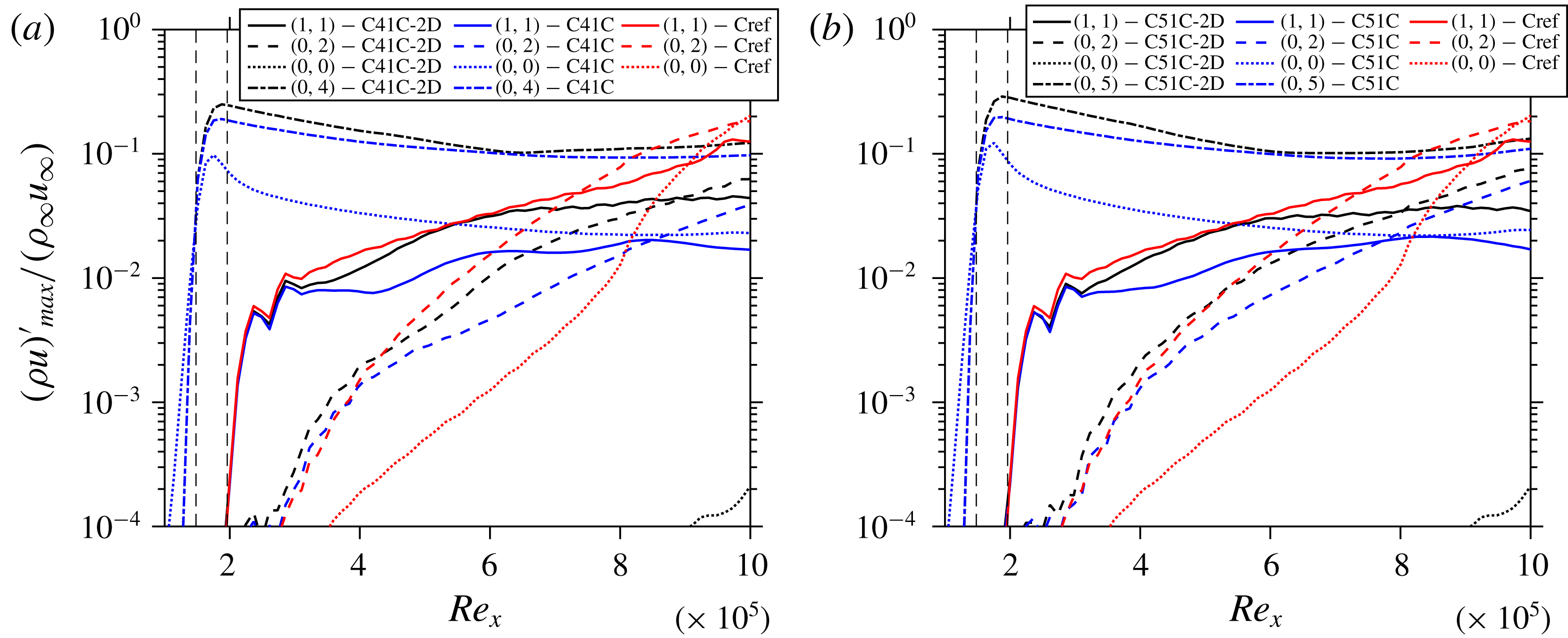
Comparison of the streamwise evolution of the maximum disturbance amplitudes of various modes for cases (a) C41C-2D with C41C and Cref, and (b) C51C-2D with C51C and Cref.
4.5 Role of the mean-flow distortion generated by the control
Here we investigate the contribution of the MFD quantitatively towards its share in the flow stabilization, cf. § 5.3 in Wassermann & Kloker (Reference Wassermann and Kloker2002). The analysis is performed as follows: the converged working cases are restarted, then the laminar baseflow is subtracted from the spanwise mean of the instantaneous flow which gives the 2-D disturbance part (2DP) of the flow including the MFD. Note that for regions where steady modes prevail, the 2DP is equal to the MFD. This 2DP is then subtracted from the instantaneous field, hence only the 3-D part remains in the flow. The same procedure is repeated at each time-step. The flow is thus deprived of any 2-D part that is nonlinearly generated. This gives interpretable results in the early stages of the scenario where the 2-D modes (2,0) and (0,0) inherent in oblique breakdown without control are not too large. Figures 12(a) and 12(b) compare the modal growth for cases with and without the 2DP with Cref for C41C and C51C, respectively. It can be seen from these figures that the initial control-mode amplitude for both (0,4) and (0,5) gets larger if the respective MFD is suppressed at equal 3-D wall forcing, i.e. the nonlinearly generated MFD reduces the generated streak mode amplitude as qualitatively expected. The initial amplitude of (1,1) is reduced by the 3-D part of the control mode, independent of the existence of the MFD. Directly downstream of the first control strip, the MFD of the control is between 8 % and 3 %, and weakens the growth rate of the fundamental oblique mode (1,1) considerably. Without MFD its growth is initially even larger than without any control part (Cref case). However, if the amplitude of MFD falls below about 3 %, its effect on the growth rate of the fundamental oblique mode (1,1) vanishes. Then, the (growth) development of the fundamental mode is the same with or without the MFD of the control, i.e. the amplitude curves run parallel with a difference caused by the initial suppressing effect of the MFD. The control streaks decay but never fall below 10 % in the cases considered, and are eventually responsible for the suppression of the fundamental mode further downstream. Therefore, it may be concluded from figure 12 that the 3-D part of the streaks causes a suppression of the fundamental mode (1,1) when their (fixed) spanwise wavelength gets lower than about 2.3 times the local boundary-layer thickness; this holds for
 $Re_{x}>5.5\times 10^{5}$
for C51C and for
 $Re_{x}>6\times 10^{5}$
for C41C; for
 $Re_{x}<5\times 10^{5}$
, the 3-D part may even cause a growth increase of (1,1). That is why a (0,3) control is here not effective for the fundamental (1,1) oblique mode, the latter being the most amplified mode as for primary instability. We note here that the ratio of spanwise wavelength to boundary-layer thickness that is found effective in control for the 3-D control part is about the same as that for optimally growing streaks, see Paredes et al. (Reference Paredes, Choudhari and Li2017). The streaks, however, decay here.
4.6 Bolstering the control
3-D representation of control strip functions at (a) FSC, and (b) SCS for C52Cn and C52Ch.

Instantaneous flow-field for C52C: contours of
 $u/u_{\infty }$
, shown at
 $y/\unicode[STIX]{x1D6FF}_{in}=0.48$
.

In order to check for an improvement of the effectiveness of transition control, another control strip is used further downstream extending from
 $Re_{x}=5.00\times 10^{5}$
to
 $Re_{x}=5.49\times 10^{5}$
for the cases C52C and C52Cn. For case C52C, the same control strip function as the first one is used. Its mathematical function is shown in figure 13(a) in a perspective view. Figure 14 shows the instantaneous flow field for C52C and it can be seen that the repetition of the strip turns out to be detrimental, resulting in earlier transition to turbulence. The cross-cut of C52C at
 $Re_{x}=8\times 10^{5}$
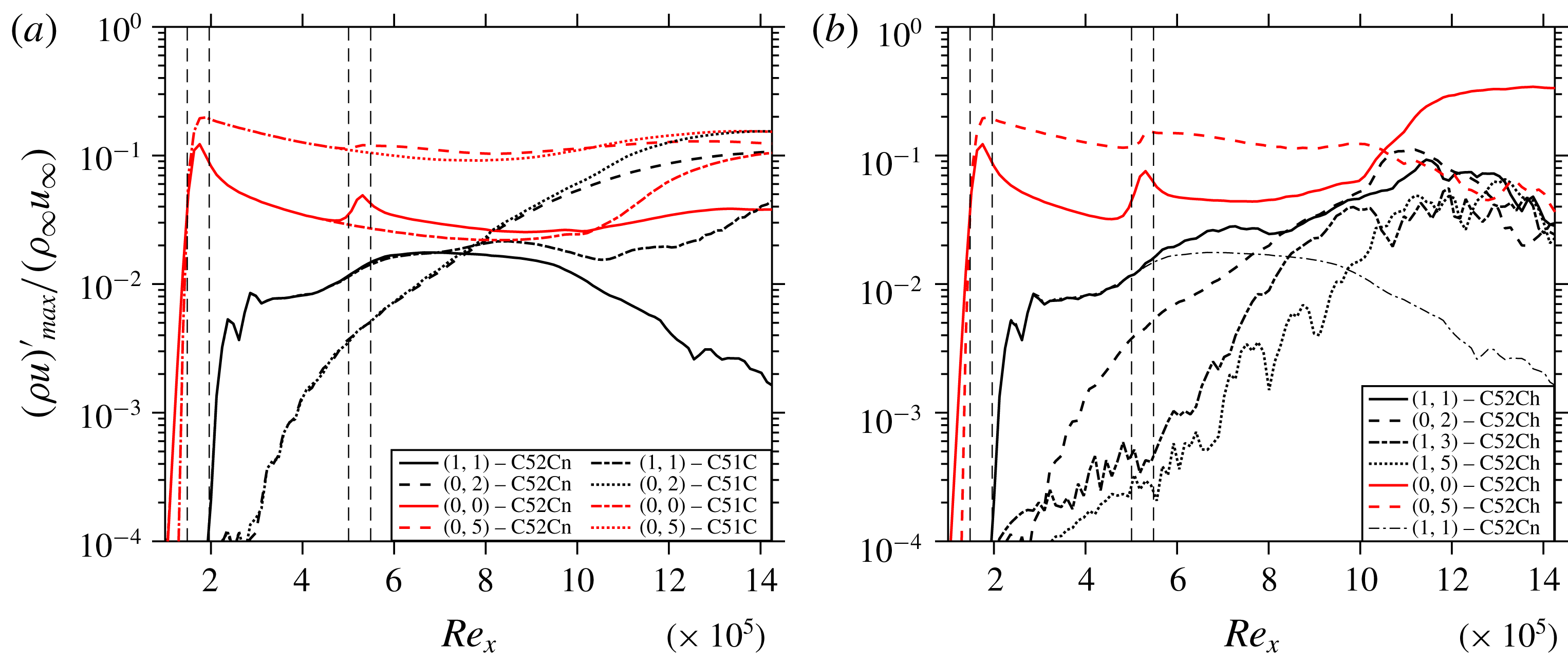
in figure 15(b) shows pronounced destabilizing low-velocity streaks in comparison to C51C in figure 5(b). Figure 14 also reveals that after the induction of the streaks from the first control strip they tend to become thinner. At the second control strip the blowing, which is of the same spanwise size of the blowing at the first strip, results in local thickening and destabilization of the streaks and hence causes transition. Note that the blowing (part of the control) induces the low-speed streaks and the wall shear is smaller at the second strip, causing the blowing to effectively penetrate deeper into the boundary-layer. This issue can be addressed by altering the second control strip in such a manner that the blowing parts of the control become narrower and remain contained inside the oncoming streaks from the first control strip. To achieve this, the disturbance function is chosen as the sum of the control mode (0,5) and its first two super-harmonics (0,10) and (0,5), each component having a third of the original amplitude to yield the same peak amplitude of the function, see figure 13(b). In case C52Cn, the flow does, indeed, not show transition, and figure 16(a) shows the effectiveness of having a second control strip, by comparing the growth of various modes for cases C51C and C52Cn. The figure documents that the increase in amplitude of (0,5) at the second control strip reinforces the beneficial MFD (0,0) at the second control strip (
 ${\approx}5\,\%$
of
 $\unicode[STIX]{x1D70C}_{\infty }u_{\infty }$
) which results in stronger suppression of the modes such as (1,1) and (0,2) for C52Cn in comparison to C51C. The instantaneous field is shown in figure 17. On comparing the streaks generated by (0,2) in C52Cn and C51C in figure 4 it can be seen that the ones for C52Cn are weaker than for C51C, which is a direct consequence of the stronger suppression of (1,1) due to the second control strip as shown in figure 16(a). If the peaky-blowing function is used for the first and second control strip, the result is the same as with the standard function for strips 1 and 2, C52C: the low-speed streaks are widened by the second strip, and the second strip is detrimental. A higher control amplitude at the second control strip leads to transition even for the peaky-blowing strip (case C52Ch). Figure 16(b) shows the modal evolution for C52Ch, and mode (1,1) is compared with case C52Cn. It is clear that just after the second control strip (1,1) grows strongly for C52Ch while it shows suppression for C52Cn indicating that most probably the mean-flow distortion generated in case C52Ch seems to be no more beneficial.
Cross-cuts of the C52C: contours of
 $u/u_{\infty }$
at (a)
 $Re_{x}=3\times 10^{5}$
, and (b)
 $Re_{x}=8\times 10^{5}$
.
Comparison of the streamwise evolution of the maximum disturbance amplitudes of various modes of cases (a) C51C and C52Cn, and (b) C52Ch and C52Cn.
Instantaneous flow-field for C52Cn: contours of
 $u/u_{\infty }$
, shown at
 $y/\unicode[STIX]{x1D6FF}_{in}=0.48$
.

(a) Generalised inflection point curves at the middle of the first control strip (
 $Re_{x}=1.722\times 10^{5}$
, red) and the middle of the second control strip (
 $Re_{x}=5.311\times 10^{5}$
, black) and (b) temperature and velocity profiles for case C51C downstream of FCS at
 $Re_{x}=3\times 10^{5}$
(red) and for C52C at SCS (black).
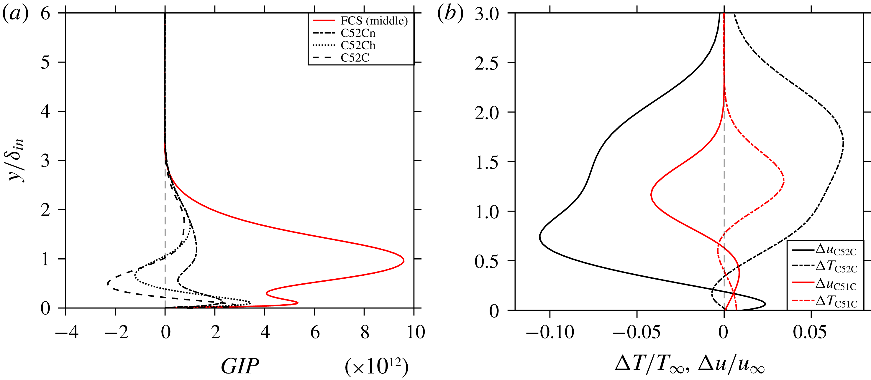
The assumption of the generation of a detrimental mean-flow distortion could be confirmed by inspecting the existence of a generalized inflection point (GIP) at the first and second control strip for all C5xCx cases. The GIP is defined as (Mack Reference Mack1984)
 $$\begin{eqnarray}GIP(y):\frac{\unicode[STIX]{x2202}\unicode[STIX]{x1D70C}}{\unicode[STIX]{x2202}y}\frac{\unicode[STIX]{x2202}u}{\unicode[STIX]{x2202}y}+\unicode[STIX]{x1D70C}\frac{\unicode[STIX]{x2202}^{2}u}{\unicode[STIX]{x2202}y^{2}}=0,\end{eqnarray}$$
and signifies the existence of an (additional) inviscid instability in the mean flow. Figure 18(a) depicts the GIP function in the middle of the first control strip (
 $Re_{x}=1.722\times 10^{5}$
) and in the middle of the second control strip (
 $Re_{x}=5.311\times 10^{5}$
) for various cases. This figure clarifies that no GIP is generated at the location of the first control strip, however, inflection points do exist at the location of the second control strip for cases C52C and C52Ch. The existence of the GIP is caused by the weaker wall shear at the second strip location due to the thicker boundary layer together with the large blowing amplitude. To assess the stabilizing role of the mean-flow distortion, the velocity and temperature profiles for mode (0,0) are plotted in figure 18(b). Here,
 $\unicode[STIX]{x0394}T=\langle T_{C51C,C52C}^{\ast }\rangle -T_{base\,flow}^{\ast }$
and
 $\unicode[STIX]{x0394}u=\langle u_{C51C,C52C}^{\ast }\rangle -u_{base\,flow}^{\ast }$
where
 $\langle \,\rangle$
signifies the spanwise and time mean. The
 $\unicode[STIX]{x0394}u$
-curve signifies that the flow is accelerated close to the wall, and decelerated in the upper two-thirds of the boundary layer, both in line to a fuller, more stable profile (cf. figure 4 of Dörr & Kloker (Reference Dörr and Kloker2017)). From the
 $\unicode[STIX]{x0394}T$
-profile it can be seen that the flow is slightly heated at the wall and cooled above. Both
 $\unicode[STIX]{x0394}u$
and
 $\unicode[STIX]{x0394}T$
point into the direction of a ‘disturbance-saturated’ mean-flow. Note that the existence of a GIP cannot be seen directly from the
 $u(y)$
and
 $T(y)$
profiles.
4.7 Effects of controlling transition
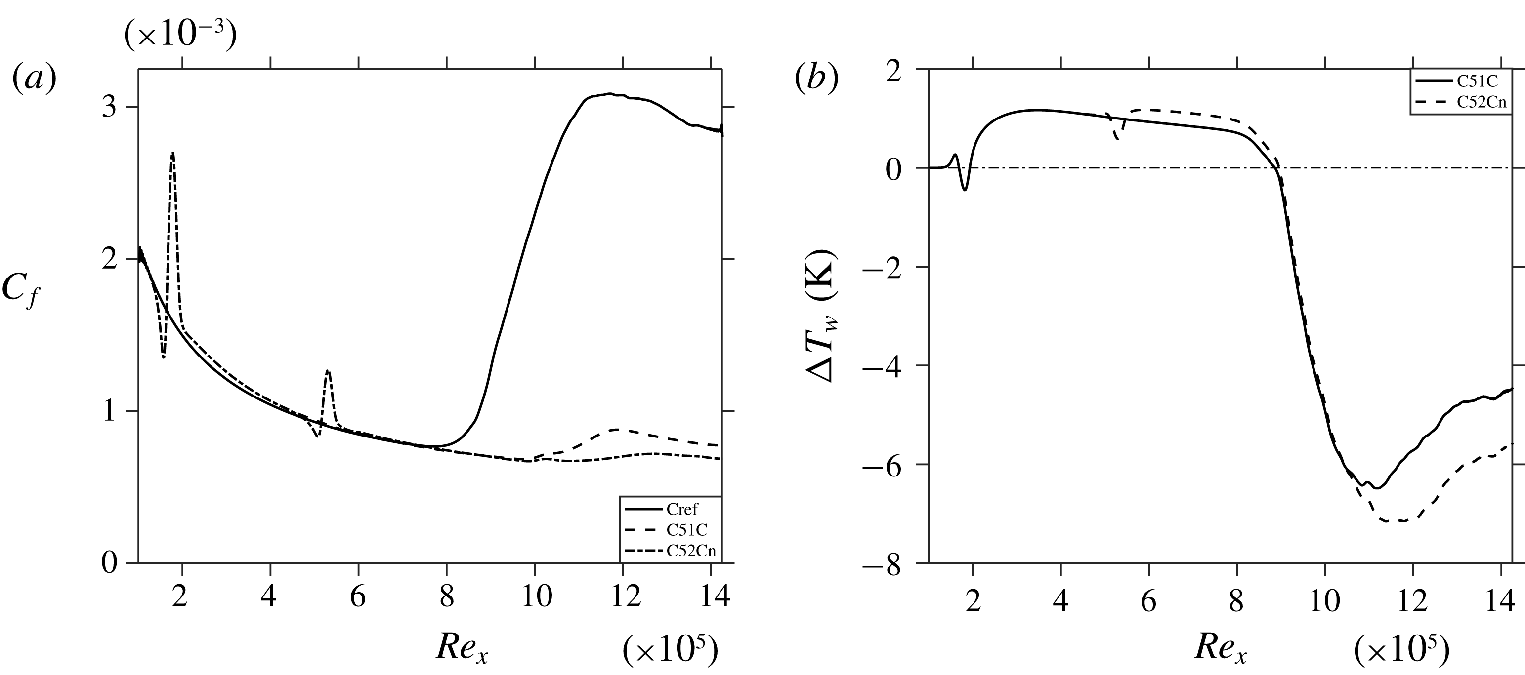
The skin-friction coefficient
 $C_{f}$
(spanwise and time mean) for cases C51C and C52Cn is compared with Cref in figure 19(a), showing the reduction of the
 $C_{f}$
values for the two controlled cases due to the absence of a turbulent region; the localized peaky increase of
 $C_{f}$
in the control strips is of minor importance. Figure 19(b) represents the temperature difference at the wall for the controlled cases,
 $\unicode[STIX]{x0394}T_{w}=\langle T_{w_{C51C,C52Cn}}\rangle -\langle T_{w_{Cref}}\rangle$
. It can be seen that due to the existence of streaks there is a slight penalty as for temperature for both cases C51C and C52Cn. Remarkably, for the turbulent portion of Cref, both cases C51C and C52Cn show a significant decrease in wall temperature, being augmented for C52Cn.
Streamwise evolution of (a)
 $C_{f}$
and (b) time and spanwise averaged temperature for corresponding controlled cases with respect to Cref.
5 Conclusions
The successful control of full oblique-type breakdown of a supersonic adiabatic boundary layer at
 $M_{\infty }=2.0$
using control streaks has been demonstrated using DNS. The investigated streaks with, in various cases, three to six times the spanwise wavenumber of the fundamental, obliquely running modes and maximal
 $\unicode[STIX]{x1D70C}u$
-amplitudes of 20 %–10 % have been introduced by steady spanwise periodic suction/blowing at the wall within one or two control strips. Generally, higher wavenumbers of the decaying streaks are found to be more effective in suppressing the unsteady most-amplified fundamental mode (1,1) but need higher initial amplitudes due to a stronger streamwise decay, and can cause a significant shock-like, detrimental steady pressure wave. The oblique-breakdown streak mode (0,2) is not much influenced directly, rather by lowering the oblique travelling modes (1,1) that feed it.
It was found that the spanwise wavelength of effective control streaks lies between 20 %–25 % of the fundamental oblique mode. Modified DNS with suppressed 2-D disturbance parts and thus MFD could show that, for the 3-D part to be effective in growth attenuation, the spanwise wavelength must be smaller than about 2.5 times the local boundary-layer thickness (
 $\unicode[STIX]{x1D706}_{control}/\unicode[STIX]{x1D6FF}<2.5$
); this value is about that of modes with optimal transient growth in theory. At the considered Reynolds number
 $Re_{x}=2\times 10^{5}$
of the first spanwise blowing–suction control strip, all steady control modes monotonically decay directly downstream of the strip, the stronger the shorter the wavelength is. Starting with the ideal
 $\unicode[STIX]{x1D706}_{control}/\unicode[STIX]{x1D6FF}$
would lead to a fast decay of the streaks and no significant control can be achieved. For the streaks found effective on the whole, the ideal
 $\unicode[STIX]{x1D706}_{control}/\unicode[STIX]{x1D6FF}$
is reached downstream near
 $Re_{x}=5.5{-}6\times 10^{5}$
when their control
 $\unicode[STIX]{x1D70C}u$
-amplitudes have decayed from initially about 20 % to 10 %, but at the same time the beneficial MFD induced falls eventually below 3 % and gets inactive. In the first streamwise part downstream of the control strip, the MFD amplitude ranges from 10 % to 3 %, and the observed oblique-mode suppression is thus solely provided by the MFD. Globally, the MFD and the 3-D part of the control contribute each with a comparable share in the reduction of the fundamental-mode amplitude.
The MFD may become maleficial (locally) if the blowing part is too strong and not pointed enough; generalized inflection points occur in the spanwise-averaged velocity profiles, invoking inviscid instability. In refreshing the control strip downstream, the oncoming low-velocity streaks must not be widened locally which would otherwise trigger transition. The initial penalties in the wall shear and wall temperature increase are marginal by the control, shifting their increase by turbulence significantly downstream. Simulations with a broader disturbance spectrum comprising higher spanwise wavenumbers
 $k$
and frequencies
 $h$
, modes (
 $h=1{-}2$
,
 $k=1{-}3$
) and significantly increased total amplitude, show that the basic suppressing mechanisms also work in this case. The additional streak modes generated (0,
 $k=4$
,6) are much closer to the control mode and were considered critical a priori, but they do not degrade the control. Whether control streaks can cope robustly with more complex disturbance situations must be subject of next-step investigations.
Acknowledgements
The authors acknowledge the access to French HPC resources provided by the French regional computing centre of Normandy (CRIANN) (grant nos 1998022 and 2017002) and Institut du développement et des ressources et informatiques scientifiques (IDRIS) under the allocation no. 2017-100752, by Grand Equipment National de Calcul Intensif (GENCI) under allocation no. A0022A10103. The funding resources are provided by European projects European Regional Development Fund (FEDER), Normandy Regional council, and NEPTUNE 1. S.S. would like to acknowledge the fruitful three-months research stay at IAG, University of Stuttgart, funded by the German Academic Exchange Service (DAAD), programme ID 57381332 (personal reference no. 91708728), hosted by M.J.K. whose ideas and support in finishing this study are appreciated.


 Open access

