2 Heterogeneous average of the stress

In this section, a method is developed to compute the average stress in heterogeneous suspensions. This study is inspired by the pioneering work of Zhang & Prosperetti (Reference Zhang and Prosperetti1994a, Reference Zhang and Prosperetti1997) towards development of ‘phase-averaging’ techniques to describe multiphase flows. We describe such suspensions mathematically as a statistically non-uniform $N$-particle ensemble; no restrictions are placed on the number, shape or compositions of the particles. The most general expression for the ensemble average of the stress $\unicode[STIX]{x1D70E}_{ij}$ at any material point $x_{i}$ in a suspension is

(2.1)$$\begin{eqnarray}\displaystyle \langle \unicode[STIX]{x1D70E}_{ij}\rangle (\boldsymbol{x})=\int \unicode[STIX]{x1D70E}_{ij}(\boldsymbol{x}|\mathscr{C})P(\mathscr{C})\,\text{d}\mathscr{C}, & & \displaystyle\end{eqnarray}$$

where $P(\mathscr{C})$ is the probability of finding the system at a configuration $\mathscr{C}$ in the phase space of all degrees of freedom in the suspension. The probability density function should be understood as an implicit function of time: $P(\mathscr{C})\equiv P(\mathscr{C},t)$. In the interest of mathematical simplicity, we will, without loss of generality, neglect explicit treatment of the time evolution of the averages.

The primary difficulty encountered in the ensemble averaging of colloidal dispersions arises from the need to incorporate and track the location of particle/fluid interfaces throughout the averaging process. Zhang & Prosperetti (Reference Zhang and Prosperetti1994a, Reference Zhang and Prosperetti1997) demonstrated that interfaces can be naturally accounted for utilizing a characteristic function $\unicode[STIX]{x1D712}(\boldsymbol{x}|\mathscr{C})$, defined as $\unicode[STIX]{x1D712}=1$ when $x_{i}$ is located in the fluid and $\unicode[STIX]{x1D712}=0$ when $x_{i}$ is inside a particle, which splits the ensemble average of any field into the sum of a fluid-phase average and particle-phase average. Utilizing this characteristic function, the ensemble-averaged stress becomes (Prosperetti Reference Prosperetti2004; Prosperetti et al. Reference Prosperetti, Zhang and Ichiki2006)

(2.2)$$\begin{eqnarray}\displaystyle \langle \unicode[STIX]{x1D70E}_{ij}\rangle (\boldsymbol{x})=\langle \unicode[STIX]{x1D712}\unicode[STIX]{x1D70E}_{ij}^{f}\rangle (\boldsymbol{x})+\langle (1-\unicode[STIX]{x1D712})\unicode[STIX]{x1D70E}_{ij}^{p}\rangle (\boldsymbol{x}), & & \displaystyle\end{eqnarray}$$

where the superscripts $f$ and $p$ represent the fluid and particle phases, respectively. We assume the suspending liquid is Newtonian with viscosity $\unicode[STIX]{x1D702}$, with the fluid stress constitutively specified as

(2.3)$$\begin{eqnarray}\displaystyle \unicode[STIX]{x1D70E}_{ij}^{f}=-p^{f}\unicode[STIX]{x1D6FF}_{ij}+2\unicode[STIX]{x1D702}\unicode[STIX]{x1D626}_{ij}^{f}, & & \displaystyle\end{eqnarray}$$

where $p$ is the thermodynamic pressure, $\unicode[STIX]{x1D626}_{ij}=u_{\{i,j\}}$ is the shear-rate tensor and $u_{i}$ is the velocity field. Substituting (2.3) into (2.2) yields

(2.4)$$\begin{eqnarray}\displaystyle \langle \unicode[STIX]{x1D70E}_{ij}\rangle =-\langle \unicode[STIX]{x1D712}p^{f}\rangle \unicode[STIX]{x1D6FF}_{ij}+2\unicode[STIX]{x1D702}\langle \unicode[STIX]{x1D712}\unicode[STIX]{x1D626}_{ij}^{f}\rangle +\langle (1-\unicode[STIX]{x1D712})\unicode[STIX]{x1D70E}_{ij}^{p}\rangle . & & \displaystyle\end{eqnarray}$$

Our point of departure from the method of Zhang & Prosperetti (Reference Zhang and Prosperetti1994a, Reference Zhang and Prosperetti1997) is our treatment the fluid- and particle-phase averages. Inspired by Batchelor (Reference Batchelor1970), we seek to convert the fluid-phase average into an average over the entire suspension. This is for both practical and heuristic reasons: measuring the stress in only the fluid phase would be difficult. Moreover, we are not interested in the stress inside the particles, but rather the additional stress arising from their presence in the fluid. Conversion to a suspension average is accomplished by extending the fluid-phase averages to the particle phase,

$$\begin{eqnarray}\displaystyle \langle \unicode[STIX]{x1D70E}_{ij}\rangle & = & \displaystyle -\langle \unicode[STIX]{x1D712}p^{f}\rangle \unicode[STIX]{x1D6FF}_{ij}+2\unicode[STIX]{x1D702}\langle \unicode[STIX]{x1D712}\unicode[STIX]{x1D626}_{ij}^{f}\rangle +\langle (1-\unicode[STIX]{x1D712})(-p^{p}\unicode[STIX]{x1D6FF}_{ij}+2\unicode[STIX]{x1D702}\unicode[STIX]{x1D626}_{ij}^{p})\rangle \nonumber\\ \displaystyle & & \displaystyle +\,\langle (1-\unicode[STIX]{x1D712})\unicode[STIX]{x1D70E}_{ij}^{p}\rangle -\langle (1-\unicode[STIX]{x1D712})(-p^{p}\unicode[STIX]{x1D6FF}_{ij}+2\unicode[STIX]{x1D702}\unicode[STIX]{x1D626}_{ij}^{p})\rangle .\nonumber\end{eqnarray}$$

This yields, with suspension averages denoted by removing superscripts,

(2.5)$$\begin{eqnarray}\displaystyle \langle \unicode[STIX]{x1D70E}_{ij}\rangle =-\langle p\rangle \unicode[STIX]{x1D6FF}_{ij}+2\unicode[STIX]{x1D702}\langle \unicode[STIX]{x1D626}_{ij}\rangle +\langle (1-\unicode[STIX]{x1D712})\unicode[STIX]{x1D6F4}_{ij}\rangle , & & \displaystyle\end{eqnarray}$$

where the particle stress

(2.6)$$\begin{eqnarray}\displaystyle \unicode[STIX]{x1D6F4}_{ij}=\unicode[STIX]{x1D70E}_{ij}^{p}+\unicode[STIX]{x1D6FF}_{ij}p^{p}-2\unicode[STIX]{x1D702}\unicode[STIX]{x1D626}_{ij}^{p} & & \displaystyle\end{eqnarray}$$

is the difference between the stress inside the particle, $\unicode[STIX]{x1D70E}_{ij}^{p}$, and the stress that would arise if the particle were replaced by pure solvent. This definition has two advantages when compared to prior definitions where the particle stress is simply defined as the average of the stress inside the particle (Prosperetti Reference Prosperetti2004; Prosperetti et al. Reference Prosperetti, Zhang and Ichiki2006). First, this quantity is identically zero for all points except those inside the particle and those bounded by the $\unicode[STIX]{x1D716}$-thin interfaces between the continuous and dispersed phase. Second, this quantity is amenable to transformation from the particle volume to its surface, where information is more readily available, allowing for the development of fundamental connections between heterogeneous flow problems and the mathematical framework of microhydrodynamics, as will be shown in § 3.

Explicit evaluation of (2.5) requires enumeration of the degrees of freedom contained in $\mathscr{C}$. Zhang & Prosperetti (Reference Zhang and Prosperetti1994a, Reference Zhang and Prosperetti1997) demonstrated that the phase space of an $N$-particle heterogeneous dispersion of spherical particles is given by the position $y_{i}^{\unicode[STIX]{x1D6FC}}$ and velocity $U_{i}^{\unicode[STIX]{x1D6FC}}$ of each particle $\unicode[STIX]{x1D6FC}$. Here, we will extend this result by considering a suspension of $N$ particles of arbitrary shape, size and concentration. To this end, we describe the geometric degrees of freedom of the particle with a generic shape parameter ${\mathcal{V}}_{p}^{\unicode[STIX]{x1D6FC}}$, which gives the set of all points bounded by $S_{p}^{\unicode[STIX]{x1D6FC}}$, the surface of particle $\unicode[STIX]{x1D6FC}$, in addition to the position $y_{i}^{\unicode[STIX]{x1D6FC}}$. In the interest of mathematical simplicity we will consider the overdamped limit, where the velocity of the particle and its surface are not independent degrees of freedom. Relaxing this assumption would leave the averaging method essentially unchanged.

Figure 1.

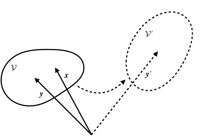
A particle moves from $\boldsymbol{y}$ and ${\mathcal{V}}$ to $\boldsymbol{y}^{\prime }$ and ${\mathcal{V}}^{\prime }$ in position and shape space by translation and deformation, while the material point $\boldsymbol{x}$ remains fixed.

As illustrated in figure 1, particles move through $y_{i}$ space by translation and through ${\mathcal{V}}_{p}$ space by rotation and deformation. This framework naturally accounts for the possibility of polydispersity in the suspension. For instance, rigid spheres of different size can be viewed as generic particles held fixed at different points in ${\mathcal{V}}_{p}$ space. For mathematical simplicity, it is assumed that each particle in the suspension is of identical material composition. This assumption is not essential to the results presented here, and is easily relaxed.

Because the particle stress (2.6) vanishes when $x_{i}$ is in the fluid, only configurations where $x_{i}$ is located in the particle, i.e. where $\boldsymbol{x}-\boldsymbol{y}^{\unicode[STIX]{x1D6FC}}\in {\mathcal{V}}_{p}^{\unicode[STIX]{x1D6FC}}$, contribute to the heterogeneous averages, yielding,

(2.7)$$\begin{eqnarray}\displaystyle \langle (1-\unicode[STIX]{x1D712})\unicode[STIX]{x1D6F4}_{ij}\rangle =\mathop{\sum }_{\unicode[STIX]{x1D6FC}}\int \int _{\boldsymbol{x}-\boldsymbol{y}^{\unicode[STIX]{x1D6FC}}\in {\mathcal{V}}_{p}^{\unicode[STIX]{x1D6FC}}}P(\boldsymbol{y}^{\unicode[STIX]{x1D6FC}},{\mathcal{V}}_{p}^{\unicode[STIX]{x1D6FC}})\langle \unicode[STIX]{x1D6F4}_{ij}\rangle (\boldsymbol{x}|\boldsymbol{y}^{\unicode[STIX]{x1D6FC}},{\mathcal{V}}_{p}^{\unicode[STIX]{x1D6FC}})\,\text{d}\boldsymbol{y}^{\unicode[STIX]{x1D6FC}}\,\text{d}{\mathcal{V}}_{p}^{\unicode[STIX]{x1D6FC}}, & & \displaystyle\end{eqnarray}$$

where $P(\boldsymbol{y}^{\unicode[STIX]{x1D6FC}},{\mathcal{V}}_{p}^{\unicode[STIX]{x1D6FC}})$ is the probability that particle $\unicode[STIX]{x1D6FC}$ is located at position $y_{i}^{\unicode[STIX]{x1D6FC}}$ with shape ${\mathcal{V}}_{p}^{\unicode[STIX]{x1D6FC}}$ and $\langle \unicode[STIX]{x1D6F4}_{ij}\rangle (\boldsymbol{x}|\boldsymbol{y}^{\unicode[STIX]{x1D6FC}},{\mathcal{V}}_{p}^{\unicode[STIX]{x1D6FC}})$ is the conditional average of $\unicode[STIX]{x1D6F4}_{ij}$ over the remainder of the configuration space $\mathscr{C}$ given that $y_{i}^{\unicode[STIX]{x1D6FC}}$ and ${\mathcal{V}}_{p}^{\unicode[STIX]{x1D6FC}}$ are fixed. Computation of this conditional average is an $(N-1)$-body problem with a solution that depends on the concentration and shape of the particles as well as properties of the flow. Noting that a particle with shape ${\mathcal{V}}_{p}$ located at a position $y_{i}$ is indistinguishable from any other particle with the same position and shape, equation (2.7) can be recast as

(2.8)$$\begin{eqnarray}\displaystyle \langle (1-\unicode[STIX]{x1D712})\unicode[STIX]{x1D6F4}_{ij}\rangle =\int \int _{\boldsymbol{x}-\boldsymbol{y}\in {\mathcal{V}}_{p}}n(\boldsymbol{y})\langle \unicode[STIX]{x1D6F4}_{ij}\rangle (\boldsymbol{x}|\boldsymbol{y},{\mathcal{V}}_{p})P({\mathcal{V}}_{p}|\boldsymbol{y})\,\text{d}\boldsymbol{y}\,\text{d}{\mathcal{V}}_{p}, & & \displaystyle\end{eqnarray}$$

where $n$ is the number density and $P({\mathcal{V}}_{p}|\boldsymbol{y})$ is the probability that a particle located at $y_{i}$ will have shape ${\mathcal{V}}_{p}$.

The expression for the particle stress derived in (2.8) is a non-local constitutive equation and is formally exact, but in practice is difficult to evaluate. Integration of (2.8) requires knowledge of the value of $\unicode[STIX]{x1D6F4}_{ij}$ at a fixed material point $x_{i}$ as the particle position $y_{i}$ is varied. However, integrals over material space are easier to manipulate because differential identities in material space may be derived using continuum balance laws, whereas identities in configuration space require manipulation of a Fokker–Planck equation. This suggests the potential convenience of recasting the configuration space integral as a material space integral. Lhuillier (Reference Lhuillier1992) demonstrated that configuration space particle-phase averages can be recast as integration in physical space through a Taylor series expansion of the integrand. Writing the average stress as

$$\begin{eqnarray}\displaystyle \langle (1-\unicode[STIX]{x1D712})\unicode[STIX]{x1D6F4}_{ij}\rangle =\int \langle (1-\unicode[STIX]{x1D712})\unicode[STIX]{x1D6F4}_{ij}\rangle (\unicode[STIX]{x1D743})\unicode[STIX]{x1D6FF}(\boldsymbol{x}-\unicode[STIX]{x1D743})\,\text{d}\unicode[STIX]{x1D743}, & & \displaystyle \nonumber\end{eqnarray}$$

and Taylor expanding the Dirac delta function about $\unicode[STIX]{x1D709}_{i}=y_{i}$ yields a material space average,

(2.9)$$\begin{eqnarray}\displaystyle \langle \unicode[STIX]{x1D6F4}_{ij}\rangle (\boldsymbol{x})=n(\boldsymbol{x})\langle \unicode[STIX]{x1D60B}_{ij}\rangle (\boldsymbol{x})-\frac{\unicode[STIX]{x2202}}{\unicode[STIX]{x2202}x_{k}}n(\boldsymbol{x})\langle \unicode[STIX]{x1D618}_{ijk}\rangle (\boldsymbol{x})+\frac{\unicode[STIX]{x2202}^{2}}{\unicode[STIX]{x2202}x_{\ell }\unicode[STIX]{x2202}x_{k}}n(\boldsymbol{x})\langle \unicode[STIX]{x1D616}_{ijk\ell }\rangle (\boldsymbol{x})+\cdots \,, & & \displaystyle\end{eqnarray}$$

where

(2.10)$$\begin{eqnarray}\displaystyle & \displaystyle \unicode[STIX]{x1D60B}_{ij}=\int _{{\mathcal{V}}_{p}}(\unicode[STIX]{x1D70E}_{ij}^{p}+p^{p}\unicode[STIX]{x1D6FF}_{ij}-2\unicode[STIX]{x1D702}\unicode[STIX]{x1D626}_{ij}^{p})\,\text{d}V, & \displaystyle\end{eqnarray}$$

(2.11)$$\begin{eqnarray}\displaystyle & \displaystyle \unicode[STIX]{x1D618}_{ijk}=\int _{{\mathcal{V}}_{p}}(\unicode[STIX]{x1D70E}_{ij}^{p}+p^{p}\unicode[STIX]{x1D6FF}_{ij}-2\unicode[STIX]{x1D702}\unicode[STIX]{x1D626}_{ij}^{p})r_{k}\,\text{d}V, & \displaystyle\end{eqnarray}$$

(2.12)$$\begin{eqnarray}\displaystyle & \displaystyle \unicode[STIX]{x1D616}_{ijk\ell }={\textstyle \frac{1}{2}}\int _{{\mathcal{V}}_{p}}(\unicode[STIX]{x1D70E}_{ij}^{p}+p^{p}\unicode[STIX]{x1D6FF}_{ij}-2\unicode[STIX]{x1D702}\unicode[STIX]{x1D626}_{ij}^{p})r_{k}r_{\ell }\,\text{d}V, & \displaystyle\end{eqnarray}$$

are the dipole, quadrupole and octupole moments of the stress in the particle, respectively, for a particle located at $x_{i}$, and $r_{i}=x_{i}-y_{i}$. The Taylor expansion corresponds to a small wavenumber expansion of the non-local constitutive equation (2.5), which will uniformly converge to the exact expression provided the macroscopic length scale over which the stress varies is larger than the particle size. The gradients of these moments provide non-local corrections to the stress arising from heterogeneity, providing a smoothly varying average between regions of different statistical properties. Higher degrees of accuracy can be obtained by including additional multipole moments after the octupole, with a commensurate increase in mathematical complexity. However, as we will show, truncating at the octupole moment typically provides sufficient accuracy for most physical systems.

3 Evaluation of the multipole moments

The multipole moments defined in (2.10)–(2.12) are volume integrals over the particle interior and the particle/fluid interfacial layer; these integrals cannot be directly evaluated in many cases due to indeterminacies in the stress in the particle interior or in the interface. For instance, the surface tension in droplets leads to an indeterminacy in the interfacial stress analogous to the indeterminacy of the pressure in incompressible fluids. This indeterminacy may be resolved by expressing the volume integrals of the stress and shear rate in terms of surface integrals of the hydrodynamic stress and velocity located just outside the interface. In this section, the conservation laws of linear and angular momentum in the particle phase presented in § 3.1 will be combined with energy methods in § 3.2 to extract tensorial symmetries that allow expression of the volume integrals as surface integrals.

3.1 Conservation laws

Conversion of the multipole moments $\unicode[STIX]{x1D60B}_{ij}$, $\unicode[STIX]{x1D618}_{ijk}$ and $\unicode[STIX]{x1D616}_{ijk\ell }$ into surface integrals is facilitated by enforcing conservation laws that can be used to derive differential identities. Expressing all information about the particle phase in terms of balance equations, rather than by constitutive equations, will avoid making unnecessarily restrictive assumptions. We first enforce conservation of momentum on the fluid phase; colloidal particles are small, so inertia is negligible on the particle scale and fluid motion is governed by the Stokes equations

(3.1a)$$\begin{eqnarray}\displaystyle & \displaystyle -p_{,i}+\unicode[STIX]{x1D702}u_{i,jj}=0, & \displaystyle\end{eqnarray}$$

(3.1b)$$\begin{eqnarray}\displaystyle & \displaystyle u_{i,i}=0. & \displaystyle\end{eqnarray}$$

Partial differentiation is denoted with commas as $a_{,i}=\unicode[STIX]{x2202}_{i}a=\unicode[STIX]{x2202}a/\unicode[STIX]{x2202}x_{i}$.

Solution of the Stokes equations in a dispersion is an inherently many-body problem requiring a closure relation for analytical treatment. A physically motivated closure relation is obtained by noting that the number of particles located a distance $r$ from a test particle is $O(\unicode[STIX]{x1D719}r^{2})$, where $\unicode[STIX]{x1D719}$ is the volume fraction. As $r\rightarrow \infty$, the number of particles become large and their combined behaviour tends towards their average,

(3.2)$$\begin{eqnarray}\displaystyle u_{i}\rightarrow \langle u_{i}\rangle \quad \text{as }r\rightarrow \infty . & & \displaystyle\end{eqnarray}$$

This closure relation introduces mathematical inconsistencies that manifest as divergent integrals when computing suspension properties (Batchelor Reference Batchelor1972; Batchelor & Green Reference Batchelor and Green1972b; Jeffrey Reference Jeffrey1973). The general approach to resolving this problem is to recast either the equations of motion or the boundary conditions in a self-consistent way by e.g. using a renormalization procedure (O’Brien Reference O’Brien1979). The motion of the fluid is set by motion of the boundaries, which can also be described by enforcing conservation of momentum, but now on the particle phase.

Particle velocity can arise in two ways. First, particles may be acted on by a body-force density $f_{i}$ and or a body-torque density $l_{i}$, so that conservation of linear and angular momentum in the particle phase is given by

(3.3a)$$\begin{eqnarray}\displaystyle & \displaystyle \unicode[STIX]{x1D70E}_{ij,j}^{p}+f_{i}=0, & \displaystyle\end{eqnarray}$$

(3.3b)$$\begin{eqnarray}\displaystyle & \displaystyle \unicode[STIX]{x1D700}_{ijk}\unicode[STIX]{x1D70E}_{kj}^{p}+l_{i}=0. & \displaystyle\end{eqnarray}$$

These expressions neglect the potential presence of dipolar or couple stresses (cf. Eringen Reference Eringen1966; Stokes Reference Stokes1966; Bleustein & Green Reference Bleustein and Green1967) arising from heterogeneity interior to the particle. However, such stresses can be safely neglected unless the particle itself is constructed from a highly heterogeneous medium (Grad Reference Grad1952; Maranganti & Sharma Reference Maranganti and Sharma2007). Second, continuity of traction and velocity across the interface

(3.4a)$$\begin{eqnarray}\displaystyle & \displaystyle \unicode[STIX]{x1D70E}_{ij}^{f}n_{j}=\unicode[STIX]{x1D70E}_{ij}^{p}n_{j}\quad \text{on }S_{p}, & \displaystyle\end{eqnarray}$$

(3.4b)$$\begin{eqnarray}\displaystyle & \displaystyle u_{i}^{f}=u_{i}^{p}\quad \text{on }S_{p}, & \displaystyle\end{eqnarray}$$

can result in momentum transport between the fluid and particle. That is, flow can carry a particle along. Note that the traction and velocity may jump across the interface in the general case. However, explicit inclusion of interfacial balance laws demonstrates that the jump condition plays no role in the suspension rheology (Nadim Reference Nadim1996) and continuity across the interface may be assumed with no loss of generality in the formulation of surface integrals. Finally, the conversion of volume integrals of the stress moments into surface integrals will by greatly facilitated by assuming the particles are incompressible

(3.5)$$\begin{eqnarray}\displaystyle u_{i,i}^{p}=0. & & \displaystyle\end{eqnarray}$$

In principle, this assumption could be relaxed by employing the theoretical methods of compressible, low Reynolds number flow (Parmar, Haselbacher & Balachandar Reference Parmar, Haselbacher and Balachandar2012).

3.2 Conversion to surface integrals

The goal of this section is to express the multipole moments $\unicode[STIX]{x1D60B}_{ij}$, $\unicode[STIX]{x1D618}_{ijk}$ and $\unicode[STIX]{x1D616}_{ijk\ell }$ in terms of four tensor types,

(3.6a)$$\begin{eqnarray}\displaystyle & \displaystyle \unicode[STIX]{x1D60D}_{ij_{1}\ldots j_{n}}^{(H,n)}=\int _{S_{p}}\unicode[STIX]{x1D70E}_{ik}^{f}n_{k}r_{j_{1}}\ldots r_{j_{n}}\,\text{d}S, & \displaystyle\end{eqnarray}$$

(3.6b)$$\begin{eqnarray}\displaystyle & \displaystyle \unicode[STIX]{x1D60D}_{ij_{1}\ldots j_{n}}^{(b,n)}=\int _{{\mathcal{V}}_{p}}f_{i}r_{j_{1}}\ldots r_{j_{n}}\,\text{d}V, & \displaystyle\end{eqnarray}$$

(3.6c)$$\begin{eqnarray}\displaystyle & \displaystyle \unicode[STIX]{x1D61D}_{ij_{1}\ldots j_{n}}^{(n)}=\int _{S_{p}}u_{i}^{f}n_{j_{1}}r_{j_{2}}\ldots r_{j_{n}}\,\text{d}S, & \displaystyle\end{eqnarray}$$

(3.6d)$$\begin{eqnarray}\displaystyle & \displaystyle \unicode[STIX]{x1D613}_{ij_{1}\ldots j_{n}}^{(n)}=\int _{{\mathcal{V}}_{p}}l_{i}r_{j_{1}}\ldots r_{j_{n}}\,\text{d}V, & \displaystyle\end{eqnarray}$$

which are the $n$th surface traction moment, the $n$th body force moment, the $n$th velocity moment and the $n$th body torque moment, respectively. The superscripts $H$ and $b$ indicate hydrodynamic and body-force moments, respectively. These tensors can be computed exactly provided that the fluid velocity, surface traction, body forces and torques acting on the particles are known, resolving any indeterminacies associated with interfacial stresses (cf. § 3).

The angular momentum balance (cf. (3.3b)) reveals that the antisymmetric part of the stress tensor may be expressed in terms of the torque pseudo-vector

$$\begin{eqnarray}\displaystyle \unicode[STIX]{x1D70E}_{[ij]}^{p}={\textstyle \frac{1}{2}}\unicode[STIX]{x1D700}_{ijk}l_{k}, & & \displaystyle \nonumber\end{eqnarray}$$

where we denote antisymmetrization of the enclosed indices with square braces, from which it follows that the portion of the multipole moments $\unicode[STIX]{x1D60B}_{ij}$, $\unicode[STIX]{x1D618}_{ijk}$ and $\unicode[STIX]{x1D616}_{ijk\ell }$ antisymmetric in $i$ and $j$ can be expressed in terms of the torque moments $\unicode[STIX]{x1D647}^{(n)}$. The remaining portions of multipole moments, those symmetric in $i$ and $j$, can be obtained by utilizing the linear momentum balance (cf. (3.3a)) to derive differential identities relating the multipole moments to the tensors defined in (3.6). We will obtain such identities using energy methods.

From appendix A, the increase in the rate of work arising from the addition of particles to the fluid is given by,

(3.7)$$\begin{eqnarray}\displaystyle \int _{S_{p}}(\langle u_{i}\rangle -U_{i}-\unicode[STIX]{x1D700}_{i\ell m}\unicode[STIX]{x1D6FA}_{\ell }r_{m})\unicode[STIX]{x1D70E}_{ij}n_{j}\,\text{d}S-\int _{S_{p}}(\langle \unicode[STIX]{x1D70E}_{ij}\rangle -\langle \unicode[STIX]{x1D6F4}_{ij}\rangle )n_{j}u_{i}^{f}\,\text{d}S, & & \displaystyle\end{eqnarray}$$

which upon application of the divergence theorem, combined with (3.3a) and the boundary conditions (3.4a)–(3.4b), yields

(3.8)$$\begin{eqnarray}\displaystyle \int _{{\mathcal{V}}_{p}}(\langle u_{i,j}\rangle +\unicode[STIX]{x1D700}_{ijk}\unicode[STIX]{x1D6FA}_{k})\unicode[STIX]{x1D70E}_{ij}^{p}\,\text{d}V-\int _{{\mathcal{V}}_{p}}(\langle \unicode[STIX]{x1D70E}_{ij}\rangle -\langle \unicode[STIX]{x1D6F4}_{ij}\rangle )u_{i,j}^{p}\,\text{d}V-\int _{V_{p}}(\langle u_{i}\rangle -U_{i}-\unicode[STIX]{x1D700}_{ijk}\unicode[STIX]{x1D6FA}_{j}r_{k})f_{i}\,\text{d}V.\quad & & \displaystyle\end{eqnarray}$$

Substituting the average stress (2.5) into (3.8), equating the resultant expression with (3.7) and rearranging yields

(3.9)$$\begin{eqnarray}\displaystyle & & \displaystyle \int _{{\mathcal{V}}_{p}}\langle \unicode[STIX]{x1D626}_{ij}\rangle (\unicode[STIX]{x1D70E}_{ij}^{p}-2\unicode[STIX]{x1D702}\unicode[STIX]{x1D626}_{ij}^{p})\,\text{d}V+\int _{{\mathcal{V}}_{p}}(\langle u_{[i,j]}\rangle +\unicode[STIX]{x1D700}_{ijk}\unicode[STIX]{x1D6FA}_{k})\unicode[STIX]{x1D70E}_{ij}^{p}\,\text{d}V\nonumber\\ \displaystyle & & \displaystyle \quad =\int _{S_{p}}(\langle u_{i}\rangle -U_{i}-\unicode[STIX]{x1D700}_{i\ell m}\unicode[STIX]{x1D6FA}_{\ell }r_{m})\unicode[STIX]{x1D70E}_{ij}^{f}n_{j}\,\text{d}S+\int _{{\mathcal{V}}_{p}}(\langle u_{i}\rangle -U_{i}-\unicode[STIX]{x1D700}_{ijk}\unicode[STIX]{x1D6FA}_{j}r_{k})f_{i}\,\text{d}V\nonumber\\ \displaystyle & & \displaystyle \qquad -\,\int _{S_{p}}(\langle \unicode[STIX]{x1D70E}_{ij}\rangle -\langle \unicode[STIX]{x1D6F4}_{ij}\rangle )n_{j}u_{i}^{f}\,\text{d}S.\end{eqnarray}$$

This gives an expression relating the stress and shear-rate fields interior to the particle with the surface traction and velocity, and is exact for all particles governed by the general conditions of § 3.1. A discussion of the relation between the body-force integral in (3.9) and conservative interparticle forces described by interaction potentials is given in B. E. Dolata and R. N. Zia (personal communication 2019). Note that here, as in § 3.1, we assume that there are no body forces acting on the fluid. Body forces localized near particle surfaces such as those arising from electric double layers, may readily be included in an extended definition of the particle pressure, permitting derivation of heterogeneous analogous of the electroviscous effect. In the presence of macroscopic applied fields, such those in electrophoresis, it may prove convenient to treat the stresses induced by these fields as quantities unrelated to the particle stress, by e.g. applying our ensemble-averaging technique to the Maxwell stress tensor.

The averaged fields in (3.9) are spatially varying tensor fields evaluated in the particle interior and at the particle surface. Inspection of the first volume integral on the left-hand side of (3.9) reveals that Taylor expanding these terms about the particle centre will yield terms matching those in in the definitions of the multipole moments (cf. (2.10)–(2.12)). We begin by Taylor expanding the pointwise-averaged velocity field, which, using the identity $u_{i,jk}=2\unicode[STIX]{x1D626}_{i(j,k)}-\unicode[STIX]{x1D626}_{jk,i}$, yields,

(3.10)$$\begin{eqnarray}\displaystyle \langle u_{i}\rangle (\boldsymbol{x})-U_{i}-\unicode[STIX]{x1D700}_{ijk}\unicode[STIX]{x1D6FA}_{j}r_{k} & = & \displaystyle \langle u_{i}\rangle (\boldsymbol{y})-U_{i}+r_{j}\langle \unicode[STIX]{x1D6FE}_{ij}\rangle (\boldsymbol{y})+{\textstyle \frac{1}{2}}r_{j}r_{k}(2\langle \unicode[STIX]{x1D626}_{i(j,k)}\rangle (\boldsymbol{y})-\langle \unicode[STIX]{x1D626}_{jk,i}\rangle (\boldsymbol{y}))\nonumber\\ \displaystyle & & \displaystyle +\,{\textstyle \frac{1}{6}}r_{j}r_{k}r_{\ell }(2\langle \unicode[STIX]{x1D626}_{i(j,k)\ell }\rangle (\boldsymbol{y})-\langle \unicode[STIX]{x1D626}_{jk,i\ell }\rangle (\boldsymbol{y})),\end{eqnarray}$$

where parentheses indicate symmetrization of the enclosed indices and where

(3.11)$$\begin{eqnarray}\displaystyle \unicode[STIX]{x1D6FE}_{ij}=u_{i,j}+\unicode[STIX]{x1D700}_{ijk}\unicode[STIX]{x1D6FA}_{k} & & \displaystyle\end{eqnarray}$$

is the relative deformation rate tensor. Next, we obtain an expression for ensemble-averaged stress, which may be obtained from a direct Taylor expansion of (2.1), yielding

$$\begin{eqnarray}\displaystyle \langle \unicode[STIX]{x1D70E}_{ij}\rangle -\langle \unicode[STIX]{x1D6F4}_{ij}\rangle & = & \displaystyle 2\unicode[STIX]{x1D702}\langle \unicode[STIX]{x1D626}_{ij}\rangle (\boldsymbol{y})+2\unicode[STIX]{x1D702}r_{k}\langle \unicode[STIX]{x1D626}_{ij,k}\rangle (\boldsymbol{y})+\unicode[STIX]{x1D702}r_{k}r_{\ell }\langle \unicode[STIX]{x1D626}_{ij,k\ell }\rangle (\boldsymbol{y})\nonumber\\ \displaystyle & & \displaystyle -\,\unicode[STIX]{x1D6FF}_{ij}r_{k}\langle p_{,k}\rangle (\boldsymbol{y})-{\textstyle \frac{1}{2}}\unicode[STIX]{x1D6FF}_{ij}r_{k}r_{\ell }\langle p_{,k\ell }\rangle (\boldsymbol{y}),\nonumber\end{eqnarray}$$

where we have set the pressure at the particle centre to zero. We assume the average pressure gradient is given by solutions of the Stokes equations $p_{,i}=\unicode[STIX]{x1D702}u_{i,jj}=2\unicode[STIX]{x1D626}_{ij,j}$; the consequence of this assumption is discussed in appendix C. Substituting the Stokesian pressure yields

(3.12)$$\begin{eqnarray}\displaystyle \langle \unicode[STIX]{x1D70E}_{ij}\rangle -\langle \unicode[STIX]{x1D6F4}_{ij}\rangle & = & \displaystyle 2\unicode[STIX]{x1D702}\langle \unicode[STIX]{x1D6FE}_{(ij)}\rangle (\boldsymbol{y})+2\unicode[STIX]{x1D702}r_{k}(\langle \unicode[STIX]{x1D626}_{ij,k}\rangle (\boldsymbol{y})-\unicode[STIX]{x1D6FF}_{ij}\langle \unicode[STIX]{x1D626}_{k\ell ,\ell }\rangle (\boldsymbol{y}))\nonumber\\ \displaystyle & & \displaystyle +\,\unicode[STIX]{x1D702}r_{k}r_{\ell }(\langle \unicode[STIX]{x1D626}_{ij,k\ell }\rangle (\boldsymbol{y})-\unicode[STIX]{x1D6FF}_{ij}\langle \unicode[STIX]{x1D626}_{km,m\ell }\rangle (\boldsymbol{y})),\end{eqnarray}$$

where $\unicode[STIX]{x1D6FE}_{(ij)}=\unicode[STIX]{x1D626}_{ij}$. We then substitute (3.10) and (3.12) into (3.9), yielding the algebraic expressions,

(3.13a)$$\begin{eqnarray}\displaystyle & \displaystyle F_{i}^{(H,0)}(\langle u_{i}^{\prime }\rangle -U_{i})=-F_{i}^{(b,0)}(\langle u_{i}\rangle -U_{i}), & \displaystyle\end{eqnarray}$$

(3.13b)$$\begin{eqnarray}\displaystyle & \displaystyle \unicode[STIX]{x1D60B}_{ij}\langle \unicode[STIX]{x1D6FE}_{ij}\rangle =(\unicode[STIX]{x1D60D}_{ij}^{(H,1)}-2\unicode[STIX]{x1D702}\unicode[STIX]{x1D61D}_{(ij)}^{(1)}+\unicode[STIX]{x1D60D}_{ij}^{(b,1)})\langle \unicode[STIX]{x1D6FE}_{ij}\rangle , & \displaystyle\end{eqnarray}$$

(3.13c)$$\begin{eqnarray}\displaystyle \unicode[STIX]{x1D618}_{ijk}\langle e_{ij,k}\rangle & = & \displaystyle (\!{\textstyle \frac{1}{2}}(2\unicode[STIX]{x1D60D}_{(ij)k}^{(H,2)}-\unicode[STIX]{x1D60D}_{kij}^{(H,2)})+{\textstyle \frac{1}{2}}(2\unicode[STIX]{x1D60D}_{(ij)k}^{(b,2)}-\unicode[STIX]{x1D60D}_{kij}^{(b,2)})\nonumber\\ \displaystyle & & \displaystyle -\,\unicode[STIX]{x1D700}_{jk\ell }\unicode[STIX]{x1D613}_{\ell i}^{(1)}-2\unicode[STIX]{x1D702}(\unicode[STIX]{x1D61D}_{ijk}^{(2)}-\unicode[STIX]{x1D6FF}_{jk}\unicode[STIX]{x1D61D}_{\ell \ell i}^{(2)})\!)\langle \unicode[STIX]{x1D626}_{ij,k}\rangle ,\end{eqnarray}$$

(3.13d)$$\begin{eqnarray}\displaystyle \unicode[STIX]{x1D616}_{ijk\ell }\langle e_{ij,k\ell }\rangle & = & \displaystyle (\!{\textstyle \frac{1}{6}}(2\unicode[STIX]{x1D60D}_{(ij)k\ell }^{(H,3)}-\unicode[STIX]{x1D60D}_{k\ell ij}^{(H,3)})+{\textstyle \frac{1}{6}}(2\unicode[STIX]{x1D60D}_{(ij)k\ell }^{(b,3)}-\unicode[STIX]{x1D60D}_{k\ell ij}^{(b,3)})\nonumber\\ \displaystyle & & \displaystyle -\,{\textstyle \frac{1}{2}}\unicode[STIX]{x1D700}_{jkm}\unicode[STIX]{x1D613}_{mi\ell }^{(2)}-\unicode[STIX]{x1D702}(\unicode[STIX]{x1D61D}_{ijk\ell }^{(3)}-\unicode[STIX]{x1D6FF}_{jk}\unicode[STIX]{x1D61D}_{mmi\ell }^{(3)})\!)\langle \unicode[STIX]{x1D626}_{ij,k\ell }\rangle .\end{eqnarray}$$

The relations above hold for every value of $\langle u_{i}\rangle$, $\langle \unicode[STIX]{x1D6FE}_{ij}\rangle$, $\langle \unicode[STIX]{x1D626}_{ij,k}\rangle$ and $\langle \unicode[STIX]{x1D626}_{ij,k\ell }\rangle$ consistent with the pointwise-averaged Cauchy momentum equation, conveniently allowing direct recovery of the hydrodynamic force from (3.13a) which balances the body force for inertia-free particles,

(3.14)$$\begin{eqnarray}\displaystyle F_{i}^{H}=F_{i}^{(H,0)}. & & \displaystyle\end{eqnarray}$$

The higher-order moments contain indeterminacies associated with index symmetries of the velocity. These indeterminacies arise directly from the governing equations, as follows. First, the pressure field is indeterminate in incompressible flow and serves as a Lagrange multiplier to enforce incompressibility. Thus, individual sources of isotropic stresses (thermodynamic and mechanical) cannot be distinguished and may be combined into a redefined indeterminate spherical stress that enforces incompressibility. Thus, while the gradient of the pressure may be computed and is completely determined by flow boundary conditions, the trace of the stress tensor can take on an infinite number of values. Second, the averaging method itself results in inherent indeterminacies because the multipole moments defined in (2.10)–(2.12) are only unique to within arbitrary solenoidal tensor fields that vanish under the divergence operators in (2.9). This is simply a higher-rank analogue of the indeterminacy associated with the scalar pressure.

The indeterminacy of the pressure is reflected in (3.13b), where, because $\unicode[STIX]{x1D6FE}_{ij}$ is traceless, $D_{ii}^{H}$ can take any value and still satisfy (3.13b). The trace of the dipole moment is dynamically insignificant because it may be included as part of an indeterminate spherical pressure, allowing us to make the convenient choice of setting the trace to zero,

(3.15)$$\begin{eqnarray}\displaystyle \unicode[STIX]{x1D60B}_{ij}=\unicode[STIX]{x1D60D}_{ij}^{(H,1)}-{\textstyle \frac{1}{3}}\unicode[STIX]{x1D6FF}_{ij}\unicode[STIX]{x1D60D}_{kk}^{(H,1)}-2\unicode[STIX]{x1D702}\unicode[STIX]{x1D61D}_{(ij)}^{(1)}+\unicode[STIX]{x1D60D}_{ij}^{(b,1)}-{\textstyle \frac{1}{3}}\unicode[STIX]{x1D6FF}_{ij}\unicode[STIX]{x1D60D}_{kk}^{(b,1)}, & & \displaystyle\end{eqnarray}$$

yielding a tensor with $8$ independent scalar components. The familiar definitions of the stresslet and hydrodynamic torque are the symmetric and antisymmetric parts of the dipole moment, respectively,

$$\begin{eqnarray}\displaystyle \unicode[STIX]{x1D60B}_{ij}=\unicode[STIX]{x1D61A}_{ij}-{\textstyle \frac{1}{2}}\unicode[STIX]{x1D700}_{ijk}L_{k}^{H}. & & \displaystyle \nonumber\end{eqnarray}$$

Next, we examine $\unicode[STIX]{x1D618}_{ijk}$. Upon noting that $\unicode[STIX]{x1D626}_{ij,k}$ is symmetric and traceless in the first two indices, application of the same argument regarding the arbitrary value of the trace yields,

(3.16)$$\begin{eqnarray}\displaystyle \unicode[STIX]{x1D618}_{ijk} & = & \displaystyle \unicode[STIX]{x1D60D}_{\{ij\}k}^{(H,2)}-{\textstyle \frac{1}{2}}\unicode[STIX]{x1D60D}_{k\{ij\}}^{(H,2)}-\unicode[STIX]{x1D702}(2\unicode[STIX]{x1D61D}_{(ij)k}^{(2)}-\unicode[STIX]{x1D6FF}_{ik}\unicode[STIX]{x1D61D}_{\ell \ell j}^{(2)}-\unicode[STIX]{x1D6FF}_{jk}\unicode[STIX]{x1D61D}_{\ell \ell i}^{(2)})\nonumber\\ \displaystyle & & \displaystyle +\,\unicode[STIX]{x1D60D}_{\{ij\}k}^{(b,2)}-{\textstyle \frac{1}{2}}\unicode[STIX]{x1D60D}_{k\{ij\}}^{(b,2)}-\unicode[STIX]{x1D6E5}_{ijmp}^{(2,2)}\unicode[STIX]{x1D700}_{mk\ell }\unicode[STIX]{x1D613}_{\ell p}^{(1)}+{\textstyle \frac{1}{2}}\unicode[STIX]{x1D700}_{ij\ell }\unicode[STIX]{x1D613}_{\ell k}^{(1)},\end{eqnarray}$$

after symmetrizing the quadrupole and rendering the first two indices traceless, and adding the antisymmetric component arising from the torque balance. Indices enclosed in curly braces have been made symmetric and traceless. We may divide the quadrupole moment into a hydrodynamic quadrupole $\unicode[STIX]{x1D618}_{ijk}^{H}$ dependent on the hydrodynamic traction and fluid velocity and a non-hydrodynamic portion dependent on body forces and torques; the hydrodynamic quadrupole is a tensor with $15$ independent components.

The process of constructing the octupole moment is more involved. Whereas indeterminacies in $\unicode[STIX]{x1D60B}_{ij}^{H}$ and $\unicode[STIX]{x1D618}_{ijk}^{H}$ were resolved by removing the trace, the two divergence operators acting on $\unicode[STIX]{x1D616}_{ijk\ell }$ in (2.9) yield a larger freedom of choice in resolving the indeterminacies of the octupole moment. As outlined in appendix C, removing these indeterminacies gives the octupole moment as the sum of the hydrodynamic octupole moment with (which contains $24$ independent components) and moments of the body forces and torques,

(3.17)$$\begin{eqnarray}\displaystyle \unicode[STIX]{x1D616}_{ijk\ell }^{H} & = & \displaystyle \mathscr{P}_{ijk\ell mpqr}({\textstyle \frac{1}{6}}(2\unicode[STIX]{x1D60D}_{(mp)qr}^{(H,3)}-\unicode[STIX]{x1D60D}_{qrmp}^{(H,3)})-\unicode[STIX]{x1D702}(\unicode[STIX]{x1D61D}_{mpqr}^{(3)}-\unicode[STIX]{x1D6FF}_{pq}\unicode[STIX]{x1D61D}_{ssmr}^{(3)}))\nonumber\\ \displaystyle & & \displaystyle +\,2\unicode[STIX]{x1D6E5}_{ijmpk\ell }^{(2,1,2)}\int _{{\mathcal{V}}_{p}}r_{m}u_{p}\,\text{d}V\nonumber\\ \displaystyle & & \displaystyle +\,\mathscr{P}_{ijk\ell mpqr}({\textstyle \frac{1}{6}}(2\unicode[STIX]{x1D60D}_{\{mp\}qr}^{(b,3)}-\unicode[STIX]{x1D60D}_{qr\{mp\}}^{(b,3)})-{\textstyle \frac{1}{2}}\unicode[STIX]{x1D700}_{mqs}\unicode[STIX]{x1D613}_{spr}^{(2)})+{\textstyle \frac{1}{4}}\unicode[STIX]{x1D700}_{ijm}\unicode[STIX]{x1D613}_{mk\ell }^{(2)},\end{eqnarray}$$

where

$$\begin{eqnarray}\displaystyle \mathscr{P}_{ijk\ell mpqr} & = & \displaystyle {\textstyle \frac{1}{2}}\unicode[STIX]{x1D6E5}_{ijmp}^{(2,2)}(\unicode[STIX]{x1D6FF}_{kq}\unicode[STIX]{x1D6FF}_{\ell r}+\unicode[STIX]{x1D6FF}_{kr}\unicode[STIX]{x1D6FF}_{\ell q})-{\textstyle \frac{1}{5}}\unicode[STIX]{x1D6E5}_{ijk\ell }^{(2,2)}\unicode[STIX]{x1D6E5}_{mpqr}^{(2,2)}\nonumber\\ \displaystyle & & \displaystyle -\,{\textstyle \frac{75}{8}}(\unicode[STIX]{x1D6E5}_{ij(k\ell )no}^{(3,3)}-{\textstyle \frac{8}{15}}\unicode[STIX]{x1D6E5}_{ijno}^{(2,2)}\unicode[STIX]{x1D6FF}_{k\ell })({\textstyle \frac{8}{7}}\unicode[STIX]{x1D6E5}_{mp(qr)no}^{(3,3)}-{\textstyle \frac{8}{15}}\unicode[STIX]{x1D6E5}_{mpno}^{(2,2)}\unicode[STIX]{x1D6FF}_{qr})\nonumber\end{eqnarray}$$

and we have added the antisymmetric component dependent on the body torques. Here, we define the tensor operator $\unicode[STIX]{x1D6E5}_{i_{1}\ldots i_{n}j_{1}\ldots j_{n}}^{(n,n)}$ as the projector of a rank-$n$ tensor onto the subspace of rank-$n$ harmonic tensors (symmetric and traceless in all indices) (Ehrentraut & Muschik Reference Ehrentraut and Muschik1998), $\mathscr{E}_{i_{1}\ldots i_{n}j_{1}\ldots j_{n}}^{(n,n)}$ as the generalized Kronecker delta that projects a rank-$n$ tensor onto a completely antisymmetric tensor (Agacy Reference Agacy1999) and $\unicode[STIX]{x1D6E5}_{ijk\ell mp}^{(2,1,2)}$ is a Clebsch–Gordan tensor (Coope Reference Coope1970) which gives the irreducible rank-two product of an antisymmetric tensor (i.e. a pseudovector) and an irreducible second-rank tensor. The functional forms of the operators may be found in appendix B.

The first term in this operator $\mathscr{P}_{ijk\ell mpqr}$ projects the octupole moment onto the correct index symmetries, while the other two terms serve to remove dynamically indeterminate parts of the stress. Note that there is a remainder velocity volume integral in the octupole which cannot be expressed as a surface integral. This term, as discussed in appendix C, is indeterminate in the Stokes equations, but may have dynamic significance in general heterogeneous flows. This remainder cannot generally be evaluated directly, but may be computed indirectly using generalized Faxén laws (B. E. Dolata and R. N. Zia, personal communication 2019) and the Lorentz reciprocal theorem. We have thus obtained all multipole moments up to fourth rank. This process can readily be extended to each rank-$n$ multipole moment, yielding a hydrodynamic moment tensor with $n(n+2)$ independent components.

We have now converted the volume integrals of the stress into integrals that are completely determinate; these expressions are exact, which may be verified by application of the divergence theorem. Note that (3.15) is identical to the expression for the dipole moment obtained by Batchelor (Reference Batchelor1970) using volume averaging procedures in homogeneous suspensions, which is satisfying, and that, in in the limit of no-slip spheres with no body torques, the quadrupole moment (3.16) reduces to that obtained by Zhou & Prosperetti (Reference Zhou and Prosperetti2020).

The body-force and torque terms (3.15)–(3.17) can be computed in principle. This is easily done for particular flows, but it is difficult to express them in explicit form for arbitrary flows. Here, we will show that they are dynamically insignificant and can be ignored. In his study of semi-dilute suspensions, Batchelor (Reference Batchelor1977) implicitly assumed that the body force (and acceleration) terms in the dipole moment derived in Batchelor (Reference Batchelor1970) are dynamically insignificant, but the origin of the claim is opaque, because this mathematical fact does not arise naturally from the volume-averaging process. This drawback of volume averaging can be overcome using the heterogeneous-averaging methods as follows. The stress in the linear and angular momentum balances (3.3a) and (3.3b) is obtained by substituting the moments above into (2.9) to obtain the particle stress, and then utilizing (2.5) to find the suspension stress, yielding

$$\begin{eqnarray}\displaystyle & \displaystyle -\langle p_{,i}\rangle +\unicode[STIX]{x1D702}\langle u_{i,jj}\rangle +\langle \unicode[STIX]{x1D6F4}_{ij,j}^{H}\rangle +\unicode[STIX]{x2202}_{j}n\langle \unicode[STIX]{x1D60D}_{ij}^{(b,1)}\rangle -{\textstyle \frac{1}{2}}\unicode[STIX]{x2202}_{j}\unicode[STIX]{x2202}_{k}n\langle \unicode[STIX]{x1D60D}_{ijk}^{(b,2)}\rangle +{\textstyle \frac{1}{6}}\unicode[STIX]{x2202}_{j}\unicode[STIX]{x2202}_{k}\unicode[STIX]{x2202}_{\ell }n\langle \unicode[STIX]{x1D60D}_{ijk\ell }^{(b,3)}\rangle +\langle \,f_{i}\rangle =0, & \displaystyle \nonumber\\ \displaystyle & \displaystyle \unicode[STIX]{x1D700}_{ijk}\langle \unicode[STIX]{x1D6F4}_{kj}^{H}\rangle +n\unicode[STIX]{x1D700}_{ijk}\langle \unicode[STIX]{x1D60D}_{kj}^{(b,1)}\rangle +\unicode[STIX]{x2202}_{j}n\langle \unicode[STIX]{x1D613}_{ij}^{(1)}\rangle -{\textstyle \frac{1}{2}}\unicode[STIX]{x2202}_{j}\unicode[STIX]{x2202}_{k}n\langle \unicode[STIX]{x1D613}_{ijk}^{(2)}\rangle +\langle l_{i}\rangle =0, & \displaystyle \nonumber\end{eqnarray}$$

where $\unicode[STIX]{x1D6F4}_{ij}^{H}$ is the particle stress arising from the hydrodynamic multipole moments and all indeterminate terms have been included in the pressure. These expressions simplify greatly by recognizing that the body-force and torque terms appear as moment expansions of $\langle f_{i}\rangle$ and $\langle l_{i}\rangle$. The average body force and torque can be expressed using the methods of § 2, yielding the moment expansions,

$$\begin{eqnarray}\displaystyle & \displaystyle \langle \,f_{i}\rangle =n\langle F_{i}^{(0,b)}\rangle -\unicode[STIX]{x2202}_{j}n\langle \unicode[STIX]{x1D60D}_{ij}^{(1,b)}\rangle +{\textstyle \frac{1}{2}}\unicode[STIX]{x2202}_{j}\unicode[STIX]{x2202}_{k}n\langle \unicode[STIX]{x1D60D}_{ijk}^{(2,b)}\rangle -{\textstyle \frac{1}{6}}\unicode[STIX]{x2202}_{j}\unicode[STIX]{x2202}_{k}\unicode[STIX]{x2202}_{\ell }n\langle \unicode[STIX]{x1D60D}_{ijk\ell }^{(3,b)}\rangle +\cdots \,, & \displaystyle \nonumber\\ \displaystyle & \displaystyle \langle l_{i}\rangle =n\langle \unicode[STIX]{x1D613}_{i}^{(0)}\rangle -\unicode[STIX]{x2202}_{j}n\langle \unicode[STIX]{x1D613}_{ij}^{(1)}\rangle +{\textstyle \frac{1}{2}}\unicode[STIX]{x2202}_{j}\unicode[STIX]{x2202}_{k}n\langle \unicode[STIX]{x1D613}_{ijk}^{(2)}\rangle +\cdots \,, & \displaystyle \nonumber\end{eqnarray}$$

which reveals much simpler conservation laws where the high-order body force and torque moments play no dynamic role,

(3.18a)$$\begin{eqnarray}\displaystyle & \displaystyle -\langle p_{,i}\rangle +\unicode[STIX]{x1D702}\langle u_{i,jj}\rangle +\langle \unicode[STIX]{x1D6F4}_{ij,j}^{H}\rangle +n\langle F_{i}^{(b,0)}\rangle =0, & \displaystyle\end{eqnarray}$$

(3.18b)$$\begin{eqnarray}\displaystyle & \displaystyle \unicode[STIX]{x1D700}_{ijk}\langle \unicode[STIX]{x1D6F4}_{kj}^{H}\rangle +n\unicode[STIX]{x1D700}_{ijk}\langle \unicode[STIX]{x1D60D}_{kj}^{(b,1)}\rangle +n\langle L_{i}^{(0)}\rangle =0. & \displaystyle\end{eqnarray}$$

Linear momentum conservation statements similar to (3.18a) have been obtained for spherical particles by Zhang & Prosperetti (Reference Zhang and Prosperetti1997), Jackson (Reference Jackson1997), and angular momentum balances similar to (3.18b) were derived by Jackson (Reference Jackson1997). Note that (3.18b) implies that the heterogeneous stress is symmetric in the absence of external (body or moment) torques, in contrast with prior works (Prosperetti Reference Prosperetti2004; Prosperetti et al. Reference Prosperetti, Zhang and Ichiki2006), which predict an antisymmetric stress, and in agreement with a recent computation of the stress in suspensions of no-slip spheres (Zhou & Prosperetti Reference Zhou and Prosperetti2020). Here, our more general approach demonstrates that these momentum balances hold for all non-inertial heterogeneous flows.

The theoretical framework presented thus far for the stress in concentrated heterogeneous suspensions is valid for particles of arbitrary shape, size and composition, as well as arbitrary sources of heterogeneity, including non-uniform shear fields, heterogeneous force fields or spatially varying volume fractions, for instance. In the next section, we apply the theory to a specific test case, a dilute suspension of spheres, in order to ensure that the theoretical framework predicts the correct physical behaviour.

4 Constitutive equations for dilute suspensions of spheres

The overall goal of this work is the development of a method to derive a general expression for the pointwise-average stress in suspensions undergoing heterogeneous flow in terms of meso- and macroscopic quantities that can be experimentally determined. A general framework that gives a pointwise-average stress, valid for dispersions of arbitrary concentration, particle shape and particle material composition, that preserves information about the underlying microscopic dynamics was derived in §§ 2 and 3. We now seek to validate the framework for a dilute suspension by demonstrating that it produces a constitutive expression for the stress consistent with experimental observations in three distinct heterogeneous flows.

To begin, we seek to replace the number density $n(\boldsymbol{x})$ appearing in (2.9), a probabilistic, microscopic description of the particle distribution prone to temporal fluctuation, with a macroscopic, ensemble-averaged description of the particle distribution. The simplest of such distributions is the spatially varying volume fraction defined by Zhang & Prosperetti (Reference Zhang and Prosperetti1994a),

(4.1)$$\begin{eqnarray}\displaystyle \unicode[STIX]{x1D719}(\boldsymbol{x})=\langle 1-\unicode[STIX]{x1D712}\rangle (\boldsymbol{x}), & & \displaystyle\end{eqnarray}$$

which is simply the probability that a material point is located inside a particle. In homogeneous dispersions, this quantity is spatially constant and recovers the standard definition of volume fraction, $\unicode[STIX]{x1D719}=n/V_{p}$. More generally, for spherical particles of radius $a$, the volume fraction may be related to the number density by integrating the number density over the spatial extent of a particle (Zhang & Prosperetti Reference Zhang and Prosperetti1994a)

(4.2)$$\begin{eqnarray}\displaystyle \unicode[STIX]{x1D719}(\boldsymbol{x})=\int _{|\boldsymbol{x}-\boldsymbol{y}|\leqslant a}n(\boldsymbol{y})\,\text{d}\boldsymbol{y}. & & \displaystyle\end{eqnarray}$$

Similar expressions for non-spherical particles may be easily obtained using the shape function ${\mathcal{V}}_{p}$ introduced in § 2. This equation can be solved for the number density, using e.g. symbolic-operator (Brenner & Haber Reference Brenner and Haber1984; Haber & Brenner Reference Haber and Brenner1984) or Fourier-transform methods, yielding an expression relating the microscopic quantity $n$ to the macroscopic observable $\unicode[STIX]{x1D719}$,

(4.3)$$\begin{eqnarray}\displaystyle n(\boldsymbol{x})=\frac{a\sqrt{\unicode[STIX]{x1D6FB}^{2}}}{4\unicode[STIX]{x03C0}a^{3}i_{1}(a\sqrt{\unicode[STIX]{x1D6FB}^{2}})}\unicode[STIX]{x1D719}(\boldsymbol{x})=\frac{3}{4\unicode[STIX]{x03C0}a^{3}}\left(1-\frac{a^{2}}{10}\unicode[STIX]{x1D6FB}^{2}+\frac{9a^{4}}{1400}\unicode[STIX]{x1D6FB}^{4}+\cdots \,\right)\unicode[STIX]{x1D719}(\boldsymbol{x}). & & \displaystyle\end{eqnarray}$$

Here, $i_{1}(z)$ is a modified spherical Bessel function of the first kind and $\sqrt{\unicode[STIX]{x1D6FB}^{2}}$ is a fractional differential operator.

A similar connection to observable quantities is also required for the multipole moments appearing in (2.9). Such a relation can be obtained by returning to the concept of energy dissipation. As discussed in § 3.2, the rate of work (and hence the energy dissipation rate) in a heterogeneous dispersion takes the form ${\dot{W}}={\mathcal{U}}^{\intercal }{\mathcal{F}}$, where ${\mathcal{U}}=\{\langle u_{i}\rangle -U_{i},\langle \unicode[STIX]{x1D6FE}_{ij}\rangle ,\langle \unicode[STIX]{x1D626}_{ij,k}\rangle ,\langle \unicode[STIX]{x1D626}_{ij,k\ell }\rangle ,\ldots \}$ is a generalized velocity vector and ${\mathcal{F}}=\{F_{i}^{H},\unicode[STIX]{x1D60B}_{ij}^{H},\unicode[STIX]{x1D618}_{ijk}^{H},\unicode[STIX]{x1D616}_{ijk\ell }^{H},\ldots \}$ is a generalized force vector. The energy dissipation rate, combined with the linearity of Stokes flow, implies the existence of a symmetric, grand resistance matrix ${\mathcal{R}}$ relating fluid and particle moments to the induced moments on the particle surface: ${\mathcal{F}}={\mathcal{R}}{\mathcal{U}}$. This grand resistance matrix, along with its index and transpose symmetries, may be expressed as,

(4.4)$$\begin{eqnarray}\displaystyle \left(\begin{array}{@{}c@{}}F_{i}^{H}\\ \unicode[STIX]{x1D60B}_{ij}^{H}\\ \unicode[STIX]{x1D618}_{ijk}^{H}\\ \unicode[STIX]{x1D616}_{ijk\ell }^{H}\end{array}\right)=\left(\begin{array}{@{}cccc@{}}\unicode[STIX]{x1D619}_{(im)}^{FU} & \unicode[STIX]{x1D619}_{mpi}^{DU} & \unicode[STIX]{x1D619}_{\{mp\}qi}^{QU} & \unicode[STIX]{x1D619}_{\{mp\}(qr)i}^{OU}\\ \unicode[STIX]{x1D619}_{ijm}^{DU} & \unicode[STIX]{x1D619}_{\text{}\underline{ij}\;\text{}\underline{mp}}^{D\unicode[STIX]{x1D6E4}} & \unicode[STIX]{x1D619}_{\{mp\}qij}^{Q\unicode[STIX]{x1D6E4}} & \unicode[STIX]{x1D619}_{\{mp\}(qr)ij}^{O\unicode[STIX]{x1D6E4}}\\ \unicode[STIX]{x1D619}_{\{ij\}km}^{QU} & \unicode[STIX]{x1D619}_{\{ij\}kmp}^{Q\unicode[STIX]{x1D6E4}} & \unicode[STIX]{x1D619}_{\text{}\underline{\{ij\}k}\;\text{}\underline{\{mp\}q}}^{QP} & \unicode[STIX]{x1D619}_{\{mp\}(qr)\{ij\}k}^{OP}\\ \unicode[STIX]{x1D619}_{\{ij\}(k\ell )m}^{OU} & \unicode[STIX]{x1D619}_{\{ij\}(k\ell )mq}^{O\unicode[STIX]{x1D6E4}} & \unicode[STIX]{x1D619}_{\{ij\}(k\ell )\{mp\}q}^{OP} & \unicode[STIX]{x1D619}_{\text{}\underline{\{ij\}(k\ell )}\;\text{}\underline{\{mp\}(qr)}}^{OM}\end{array}\right)\left(\begin{array}{@{}c@{}}\langle u_{m}\rangle -U_{m}\\ \langle \unicode[STIX]{x1D6FE}_{mp}\rangle \\ \langle \unicode[STIX]{x1D626}_{mp,q}\rangle \\ \langle \unicode[STIX]{x1D626}_{mp,qr}\rangle \end{array}\right), & & \displaystyle\end{eqnarray}$$

where underbars represent a block symmetric tensor, i.e. $\unicode[STIX]{x1D608}_{\text{}\underline{i_{1}\ldots i_{n}}\;\text{}\underline{j_{1}\ldots j_{n}}}=\unicode[STIX]{x1D608}_{\text{}\underline{j_{1}\ldots j_{n}}\;\text{}\underline{i_{1}\ldots i_{n}}}$, and $\langle u_{i}\rangle$, $\langle \unicode[STIX]{x1D6FE}_{ij}\rangle$, $\langle \unicode[STIX]{x1D626}_{ij,k}\rangle$ and $\langle \unicode[STIX]{x1D626}_{ij,k\ell }\rangle$ are evaluated at the particle centre. All solutions to the Stokes equations, including those from which the grand resistance matrix arises, must produce positive energy dissipation, meaning we must have the quadratic form ${\mathcal{U}}^{\intercal }{\mathcal{R}}{\mathcal{U}}>0$. One way to enforce this is to require a positive definite grand resistance matrix. In the present case, the grand resistance matrix may not be positive definite, because the ${\mathcal{U}}$ that satisfies the pointwise-averaged Cauchy momentum equation gives a shear rate $\langle \unicode[STIX]{x1D626}_{ij}\rangle$ that cannot be varied independently from its gradients $\langle \unicode[STIX]{x1D626}_{ij,k}\rangle$ and $\langle \unicode[STIX]{x1D626}_{ij,k\ell }\rangle$. Indeed, these are coupled by prescription in order to smoothly connect heterogeneous flow and stress variations. However, all flows encoded into ${\mathcal{U}}$ are obtained from an expansion of an equation of motion that generates positive energy dissipation; hence all grand resistance matrices derived using the methods of this paper automatically produce positive dissipation. That is, any flow ${\mathcal{U}}$ that passes through ${\mathcal{R}}$ to give ${\dot{W}}<0$ disobeys conservation of momentum and is not physically realizable, and thus presents no concern.

A non-positive definite grand resistance matrix is not necessarily invertible. However, any sub-blocks for which well-posed boundary value problems exist for both the force moment and velocity derivative must be positive definite and hence invertible. For instance, well-posed boundary value problems exist for both $F_{i}^{H}$ and $U_{i}$ meaning the sub-block involving $\unicode[STIX]{x1D64D}^{FU}$ must be positive definite. However, $\unicode[STIX]{x1D64D}^{QP}$ may not necessarily be invertible because there exists no well-posed physical boundary condition for $\unicode[STIX]{x1D618}_{ijk}^{H}$.

Provided the resistance tensors are known, we can now express the multipole moments in terms of the observables $\langle u_{i}\rangle -\langle U_{i}\rangle$, $\langle \unicode[STIX]{x1D6FE}_{ij}\rangle$, $\langle \unicode[STIX]{x1D626}_{ij,k}\rangle$ and $\langle \unicode[STIX]{x1D626}_{ij,k\ell }\rangle$. Note that the relative particle velocity $\langle u_{i}\rangle -\langle U_{i}\rangle$ can be difficult to measure in principle, and it will often prove convenient to remove it by supplementing the grand resistance matrix with a force balance on the particle. The resistance tensors for spherical particles of arbitrary composition can be obtained from solutions of six linearly independent microhydrodynamics problems, as demonstrated in appendix D. The resulting hydrodynamic resistance tensors are,

(4.5a)$$\begin{eqnarray}\displaystyle & \displaystyle \unicode[STIX]{x1D619}_{(ij)}^{FU}=\frac{4\unicode[STIX]{x03C0}a}{3}f_{1}\unicode[STIX]{x1D6FF}_{ij}, & \displaystyle\end{eqnarray}$$

(4.5b)$$\begin{eqnarray}\displaystyle & \displaystyle \unicode[STIX]{x1D619}_{\text{}\underline{ij}\;\text{}\underline{k\ell }}^{D\unicode[STIX]{x1D6E4}}=\frac{8\unicode[STIX]{x03C0}\unicode[STIX]{x1D702}a^{3}}{3}(s_{1}\unicode[STIX]{x1D6E5}_{ijk\ell }^{(2,2)}+\ell _{1}\mathscr{E}_{ijk\ell }^{(2,2)}), & \displaystyle\end{eqnarray}$$

(4.5c)$$\begin{eqnarray}\displaystyle & \displaystyle \unicode[STIX]{x1D619}_{\{ij\}k\ell }^{QU}=\frac{8\unicode[STIX]{x03C0}a^{3}}{3}f_{2}\unicode[STIX]{x1D6E5}_{ijk\ell }^{(2,2)}, & \displaystyle\end{eqnarray}$$

(4.5d)$$\begin{eqnarray}\displaystyle & \displaystyle \unicode[STIX]{x1D619}_{\text{}\underline{\{ij\}k}\;\text{}\underline{\{\ell m\}p}}^{QP}=\frac{8\unicode[STIX]{x03C0}\unicode[STIX]{x1D702}a^{5}}{3}(q_{1}^{I}\unicode[STIX]{x1D6E5}_{ijk\ell mp}^{(3,3)}+4q_{1}^{R}\unicode[STIX]{x1D6E5}_{ij\unicode[STIX]{x1D6FC}\unicode[STIX]{x1D6FD}no}^{(2,1,2)}\mathscr{E}_{\unicode[STIX]{x1D6FC}\unicode[STIX]{x1D6FD}k\unicode[STIX]{x1D6FE}\unicode[STIX]{x1D701}p}^{(3,3)}\unicode[STIX]{x1D6E5}_{\ell m\unicode[STIX]{x1D6FE}\unicode[STIX]{x1D701}no}^{(2,1,2)}+\frac{3q_{1}^{D}}{5}\unicode[STIX]{x1D6E5}_{ijkr}^{(2,2)}\unicode[STIX]{x1D6E5}_{\ell mpr}^{(2,2)}), & \displaystyle\end{eqnarray}$$

(4.5e)$$\begin{eqnarray}\displaystyle & \displaystyle \unicode[STIX]{x1D619}_{\{ij\}(k\ell )mp}^{O\unicode[STIX]{x1D6E4}}=\frac{4\unicode[STIX]{x03C0}\unicode[STIX]{x1D702}a^{5}}{3}\left(s_{2}\unicode[STIX]{x1D6E5}_{ijmp}^{(2,2)}\unicode[STIX]{x1D6FF}_{k\ell }+\frac{2(5\ell _{1}-3)}{15}\unicode[STIX]{x1D6E5}_{ijmpk\ell }^{(2,1,2)}\right), & \displaystyle\end{eqnarray}$$

(4.5f)$$\begin{eqnarray}\displaystyle & \displaystyle \unicode[STIX]{x1D619}_{ijk}^{DU}=\unicode[STIX]{x1D619}_{\{ij\}k\ell m}^{Q\unicode[STIX]{x1D6E4}}=\unicode[STIX]{x1D619}_{\{ij\}(k\ell )m}^{OU}=\unicode[STIX]{x1D619}_{\{ij\}(k\ell )\{mp\}q}^{OP}=0, & \displaystyle\end{eqnarray}$$

$f_{1}$

$f_{2}$

$\ell _{1}$

$s_{1}$

$s_{2}$

$q_{1}^{D}$

$q_{1}^{R}$

$q_{1}^{I}$

$f_{1}=9/2$

$s_{1}=5/2$

$\ell _{1}=3/2$

$\unicode[STIX]{x1D64D}^{OM}$

$O(\unicode[STIX]{x1D702}a^{4}\unicode[STIX]{x1D719}\unicode[STIX]{x1D626}_{ij,kk\ell \ell })$

$O(a^{4}/L^{4})$

$L$

(4.6)$$\begin{eqnarray}\displaystyle m\frac{\text{d}U_{i}}{\text{d}t}=F_{i}^{H}+F_{i}^{(b,0)}+F_{i}^{\prime }=\frac{4\unicode[STIX]{x03C0}af_{1}}{3}(\langle u_{i}\rangle -U_{i})+\frac{4\unicode[STIX]{x03C0}a^{3}f_{2}}{3}\langle u_{i,jj}\rangle +F_{i}^{(b,0)}+F_{i}^{\prime }, & & \displaystyle\end{eqnarray}$$

where $F_{i}^{\prime }$, the fluctuating force arising from Brownian motion and mean-field interactions with the other particles, has zero mean. The inertial term may be computed by re-expressing the total derivative as partial derivatives,

(4.7)$$\begin{eqnarray}\displaystyle m\left\langle \frac{\text{d}U_{i}}{\text{d}t}\right\rangle =m\frac{\unicode[STIX]{x2202}}{\unicode[STIX]{x2202}t}\langle U_{i}\rangle +m\frac{\unicode[STIX]{x2202}}{\unicode[STIX]{x2202}x_{j}}\langle U_{i}U_{j}\rangle . & & \displaystyle\end{eqnarray}$$

The first term on the right-hand side is negligible when the Stokes number is small. The second term corresponds to velocity fluctuations arising from Brownian motion, and is found to have the value $kT\unicode[STIX]{x2202}_{i}\ln n$ from the Fokker–Planck equation (cf. Wilemski Reference Wilemski1976), where $k$ is Boltzmann’s constant and $T$ is the temperature.

We now have enough information to compute a constitutive equation for the suspension flow valid in the low Stokes and particle Reynolds number regime. The procedure is as follows: first, resistance tensors in (4.5), which are fully defined once particle boundary conditions are set, are used to compute the multipole moments $\unicode[STIX]{x1D60B}_{ij}^{H}$, $\unicode[STIX]{x1D618}_{ijk}^{H}$ and $\unicode[STIX]{x1D616}_{ijk\ell }^{H}$, whereupon the force balance (4.6) is employed to eliminate terms linear in $\langle u_{i}\rangle -U_{i}$. The resultant expressions are then substituted into (2.9), the pointwise-averaged particle stress. At this point, the number density is expressed in terms of the volume fraction using (4.3), which must be truncated to the same order as the octupole moment $\unicode[STIX]{x1D616}_{ijk\ell }^{H}$, resulting in the following constitutive equation:

(4.8)$$\begin{eqnarray}\displaystyle \unicode[STIX]{x1D70E}_{ij} & = & \displaystyle -p\unicode[STIX]{x1D6FF}_{ij}+2\unicode[STIX]{x1D702}^{eff}\unicode[STIX]{x1D626}_{ij}-2\unicode[STIX]{x1D707}\unicode[STIX]{x1D626}_{ij,kk}-2\unicode[STIX]{x1D702}_{v}\unicode[STIX]{x1D700}_{ijk}(\unicode[STIX]{x1D714}_{k}-\unicode[STIX]{x1D6FA}_{k})-2\unicode[STIX]{x1D707}_{s}\unicode[STIX]{x1D700}_{ijk}\unicode[STIX]{x1D714}_{k,\ell \ell }\nonumber\\ \displaystyle & & \displaystyle +\,2\unicode[STIX]{x1D6FC}_{I}\unicode[STIX]{x1D719}_{,k}u_{\{i,jk\}}+\frac{2\unicode[STIX]{x1D6FC}_{R}}{3}(\unicode[STIX]{x1D700}_{ki\ell }\unicode[STIX]{x1D714}_{\{\ell ,j\}}+\unicode[STIX]{x1D700}_{kj\ell }\unicode[STIX]{x1D714}_{\{\ell ,i\}})\unicode[STIX]{x1D719}_{,k}+\frac{3\unicode[STIX]{x1D6FC}_{D}}{5}\unicode[STIX]{x1D719}_{,k}\unicode[STIX]{x1D6E5}_{ijk\ell }^{(2,2)}u_{\ell ,mm}\nonumber\\ \displaystyle & & \displaystyle -\,2(\unicode[STIX]{x1D700}_{j\ell k}\unicode[STIX]{x2202}_{i}\unicode[STIX]{x2202}_{\ell }+\unicode[STIX]{x1D700}_{i\ell k}\unicode[STIX]{x2202}_{j}\unicode[STIX]{x2202}_{\ell })\unicode[STIX]{x1D707}_{s}(\unicode[STIX]{x1D714}_{k}-\unicode[STIX]{x1D6FA}_{k})+2\unicode[STIX]{x2202}_{k}\unicode[STIX]{x1D701}\unicode[STIX]{x1D6E5}_{ijk\ell }^{(2,2)}f_{\ell }^{(b,0)}-\frac{2kT}{V_{p}}\unicode[STIX]{x2202}_{k}\unicode[STIX]{x1D701}\unicode[STIX]{x1D6E5}_{ijk\ell }^{(2,2)}\unicode[STIX]{x2202}_{\ell }\ln \unicode[STIX]{x1D719},\qquad\end{eqnarray}$$

where ensemble averages have been dropped for ease of readability, $f_{i}^{(0)}=F_{i}^{(0,b)}/V_{p}$ is the average body force per unit volume and we have excluded all terms of $O(\unicode[STIX]{x1D702}\unicode[STIX]{x1D719}a^{4}\unicode[STIX]{x1D626}_{ij,kk\ell \ell })$ and higher. The transport coefficients emerge naturally as

(4.9a)$$\begin{eqnarray}\displaystyle & \displaystyle \unicode[STIX]{x1D702}^{eff}=\unicode[STIX]{x1D702}\left(1+s_{1}\unicode[STIX]{x1D719}-\left(\frac{a^{2}}{10}s_{1}-\frac{a^{2}}{2}s_{2}\right)\unicode[STIX]{x1D719}_{,kk}\right), & \displaystyle\end{eqnarray}$$

(4.9b)$$\begin{eqnarray}\displaystyle & \displaystyle \unicode[STIX]{x1D707}=\unicode[STIX]{x1D702}a^{2}\unicode[STIX]{x1D719}\left(\frac{8}{15}q_{1}^{I}+\frac{3}{10}q_{1}^{D}+\frac{1}{6}q_{1}^{R}-\frac{f_{2}^{2}}{f_{1}}-s_{2}\right), & \displaystyle\end{eqnarray}$$

(4.9c)$$\begin{eqnarray}\displaystyle & \displaystyle \unicode[STIX]{x1D702}_{v}=\unicode[STIX]{x1D702}\ell _{1}\left(\unicode[STIX]{x1D719}-\frac{a^{2}}{10}\unicode[STIX]{x1D719}_{,kk}\right), & \displaystyle\end{eqnarray}$$

(4.9d)$$\begin{eqnarray}\displaystyle & \displaystyle \unicode[STIX]{x1D707}_{s}=\unicode[STIX]{x1D702}a^{2}\unicode[STIX]{x1D719}\frac{5\ell _{1}-3}{30}, & \displaystyle\end{eqnarray}$$

(4.9e)$$\begin{eqnarray}\displaystyle & \displaystyle \unicode[STIX]{x1D6FC}_{I}=\unicode[STIX]{x1D702}a^{2}(s_{2}-q_{1}^{I}), & \displaystyle\end{eqnarray}$$

(4.9f)$$\begin{eqnarray}\displaystyle & \displaystyle \unicode[STIX]{x1D6FC}_{R}=\unicode[STIX]{x1D702}a^{2}(s_{2}-q_{1}^{R}), & \displaystyle\end{eqnarray}$$

(4.9g)$$\begin{eqnarray}\displaystyle & \displaystyle \unicode[STIX]{x1D6FC}_{D}=\unicode[STIX]{x1D702}a^{2}\left(\frac{10}{3}\frac{f_{2}^{2}}{f_{1}}+s_{2}-q_{1}^{D}\right), & \displaystyle\end{eqnarray}$$

(4.9h)$$\begin{eqnarray}\displaystyle & \displaystyle \unicode[STIX]{x1D701}=a^{2}\frac{f_{2}}{f_{1}}\unicode[STIX]{x1D719}. & \displaystyle\end{eqnarray}$$

$\unicode[STIX]{x1D702}^{eff}$

$\unicode[STIX]{x1D702}_{v}$

$\unicode[STIX]{x1D707}$

$\unicode[STIX]{x1D707}_{s}$

$\unicode[STIX]{x1D6FC}_{I}$

$\unicode[STIX]{x1D6FC}_{R}$

$\unicode[STIX]{x1D6FC}_{D}$

$\unicode[STIX]{x1D701}$

$\ln \unicode[STIX]{x1D719}$

$\unicode[STIX]{x1D719}$

This constitutive equation is quite different from prior constitutive equations or transport equations for colloids (Jackson Reference Jackson1997; Zhang & Prosperetti Reference Zhang and Prosperetti1997; Prosperetti Reference Prosperetti2004) that include the particle velocity (as a kinematic variable). These prior works point out that (using our notation) $\unicode[STIX]{x1D64D}^{QU}\sim \unicode[STIX]{x1D702}a^{3}$ whereas $\unicode[STIX]{x1D64D}^{QP}\sim \unicode[STIX]{x1D64D}^{O\unicode[STIX]{x1D6E4}}\sim a^{5}\unicode[STIX]{x1D702}$, and thus they assert that the leading-order heterogeneous correction to the stress arises from the velocity difference $\langle u_{i}\rangle -\langle U_{i}\rangle$. However, conservation of momentum on a particle as given by (4.6) shows that $\unicode[STIX]{x1D64D}^{QU}$ enters the momentum balance at the same order as $\unicode[STIX]{x1D64D}^{QP}$ and $\unicode[STIX]{x1D64D}^{O\unicode[STIX]{x1D6E4}}$, and thus these terms cannot be neglected. Jin et al. (Reference Jin, Kang, Ahn, Briels and Dhont2018) have correctly included these higher-order couplings in their derivation of the value of $\unicode[STIX]{x1D707}$ for dilute suspensions of no-slip spheres. However, their results were limited to computation of $\unicode[STIX]{x1D707}$ only and, as will be shown below, errors in their analysis resulted in a value of the shear-curvature viscosity $\unicode[STIX]{x1D707}=\unicode[STIX]{x1D702}a^{2}\unicode[STIX]{x1D719}/10$ inconsistent with physical constraints on $\unicode[STIX]{x1D707}$.

Thermodynamic physical constraints on $\unicode[STIX]{x1D707}$ from continuum constitutive equations suggest a positive value of $\unicode[STIX]{x1D707}$ (Eringen Reference Eringen1966; Stokes Reference Stokes1966; Bleustein & Green Reference Bleustein and Green1967) in contrast with experimental observations of $\unicode[STIX]{x1D707}<0$. For instance, the functional form of the pair diffusivity measured in microrheology experiments of F-actin networks (Sonn-Segev et al. Reference Sonn-Segev, Bernheim-Groswasser, Diamant and Roichman2014) can be shown to be consistent with negative values of $\unicode[STIX]{x1D707}$ when compared with point force velocity solutions of e.g. the micropolar fluid (Ramkissoon & Majumdar Reference Ramkissoon and Majumdar1976). Similar theory/experiment conflicts exist in solid mechanics (Maranganti & Sharma Reference Maranganti and Sharma2007; Askes & Aifantis Reference Askes and Aifantis2011), where continuum thermodynamic arguments again predict positive values of the elastic equivalents of $\unicode[STIX]{x1D707}$, whereas lattice models (Chang & Gao Reference Chang and Gao1995), molecular dynamics simulations (Maranganti & Sharma Reference Maranganti and Sharma2007) and experimental measurements (Jakata & Every Reference Jakata and Every2008) all predict negative $\unicode[STIX]{x1D707}<0$.

We believe that the weight of evidence suggests that $\unicode[STIX]{x1D707}<0$, in contrast with the thermodynamic predictions of $\unicode[STIX]{x1D707}>0$, suggesting that the computation of Jin et al. (Reference Jin, Kang, Ahn, Briels and Dhont2018) is incorrect. This conflict can be reconciled by recognizing that the thermodynamic constraints in the continuum models arise from an assumption that constitutive models employing $\unicode[STIX]{x1D707}$ are exact descriptions over all length scales. It is well known that $\unicode[STIX]{x1D707}>0$ leads to thermodynamic instabilities only for very large shear-rate gradients (Askes & Aifantis Reference Askes and Aifantis2011). However, the heterogeneous constitutive models discussed here are inherently perturbative in nature, with $\unicode[STIX]{x1D707}\unicode[STIX]{x1D6FB}^{2}\unicode[STIX]{x1D626}_{ij}$ providing the leading-order correction for non-local behaviour in the shear rate. Thus, very large gradients are outside the range of validity of the results and application of thermodynamic constraints at arbitrary length scales will lead to spurious results. A similar phenomenon has been seen in weakly nonlinear constitutive equations such as the second-order fluid models, where thermodynamic bounds on coefficients derived at high shear rates lead to negative relaxation times (Aksel Reference Aksel2002).

Constraints on other model parameters may be obtained by comparing our model to experiments and simulation. Stokesian dynamics simulations of colloids in a rheometer of gap width $H$ have reported that the high-frequency viscosity of the suspensions increases with decreasing $H$ (Swan & Brady Reference Swan and Brady2011). Similar behaviours are observed in the steady shear viscosity of polydisperse suspensions, where polydispersity prevents shear-induced ordering (Ramaswamy et al. Reference Ramaswamy, Lin, Leahy, Ness, Fiore, Swan and Cohen2017). The influence of confinement on stress obtained from our heterogeneous-averaging method can be found by volume averaging of the effective viscosity in (4.9) over the interior of a rheometer of width $H$, which yields,

$$\begin{eqnarray}\displaystyle \frac{1}{V}\int \unicode[STIX]{x1D702}^{eff}\,\text{d}V=\unicode[STIX]{x1D702}\left(1+\unicode[STIX]{x1D719}s_{1}-\frac{a}{H}\left(\frac{a}{10}s_{1}-\frac{a}{2}s_{2}\right)\frac{\unicode[STIX]{x2202}\unicode[STIX]{x1D719}}{\unicode[STIX]{x2202}n}\right), & & \displaystyle \nonumber\end{eqnarray}$$

where $\unicode[STIX]{x2202}\unicode[STIX]{x1D719}/\unicode[STIX]{x2202}n$ is the normal derivative of the volume fraction evaluated at the rheometer wall. Because the volume fraction is identically zero at the wall and increases towards the bulk, this normal derivative is always negative. Thus, replicating observed increases in viscosity with decreasing gap width requires that

(4.10)$$\begin{eqnarray}\displaystyle s_{1}\geqslant 5s_{2}. & & \displaystyle\end{eqnarray}$$

As will be shown below, this is equivalent to the statement that of all dilute suspensions of spherical particles of a given material composition, solid spheres with no-slip boundary conditions maximize the energy dissipation.

Constraints on the anisotropy coefficients $\unicode[STIX]{x1D6FC}_{I}$, $\unicode[STIX]{x1D6FC}_{D}$ and $\unicode[STIX]{x1D6FC}_{R}$ may be found by examining the problem of pressure-driven flow in a pipe. It is well known that particles tend to move toward the centreline in pressure-driven flow of particle laden dispersions at vanishingly small Reynolds number (Koh et al. Reference Koh, Hookham and Leal1994; Lyon & Leal Reference Lyon and Leal1998a,Reference Lyon and Lealb; Frank et al. Reference Frank, Anderson, Weeks and Morris2003); the underlying mechanism is shear-induced migration, which is distinct from the inertial Segré–Silberberg effect where particles accumulate in a region located between the wall and the centreline (Segre & Silberberg Reference Segre and Silberberg1961). In order to be consistent with these experiments, our model must predict particle migration. At low volume fractions, it is observed that the velocity profile in the pipe remains nearly parabolic despite particle migration (Koh et al. Reference Koh, Hookham and Leal1994; Frank et al. Reference Frank, Anderson, Weeks and Morris2003), whereas it exhibits significant blunting in concentrated suspensions (Lyon & Leal Reference Lyon and Leal1998a,Reference Lyon and Lealb). We will, in light of these experimental observations, examine the stress tensor predicted by (4.8) for a parabolic velocity profile, and determine the values of $\unicode[STIX]{x1D6FC}_{I}$, $\unicode[STIX]{x1D6FC}_{R}$ and $\unicode[STIX]{x1D6FC}_{D}$ for which particle migration occurs.

The position-dependent part of pressure-driven flow through a planar or circular duct may be represented as

(4.11)$$\begin{eqnarray}\displaystyle u_{i}(\boldsymbol{x})={\textstyle \frac{1}{2}}\unicode[STIX]{x1D617}_{ijk}x_{j}x_{k},\quad \unicode[STIX]{x1D617}_{ijk}=m_{i}(n_{i}n_{j}+\unicode[STIX]{x1D706}q_{i}q_{j}), & & \displaystyle\end{eqnarray}$$

where $n_{i}$, $n_{i}$ and $q_{i}$ are three mutually orthogonal vectors and $\unicode[STIX]{x1D706}$ controls the shape of the pipe; $\unicode[STIX]{x1D706}=0$ corresponds to planar Poiseuille flow and $\unicode[STIX]{x1D706}=1$ corresponds to a circular duct. Substituting (4.11) into (4.8) yields

(4.12)$$\begin{eqnarray}\displaystyle \unicode[STIX]{x1D70E}_{ij}=-p\unicode[STIX]{x1D6FF}_{ij}+2P_{(ij)k}\left[\unicode[STIX]{x1D702}^{eff}x_{k}+\left(\frac{2(4-\unicode[STIX]{x1D706})}{15}\unicode[STIX]{x1D6FC}_{I}+\frac{1-\unicode[STIX]{x1D706}}{6}\unicode[STIX]{x1D6FC}_{R}+\frac{3(1+\unicode[STIX]{x1D706})}{10}\unicode[STIX]{x1D6FC}_{D}\right)\unicode[STIX]{x1D719}_{,k}\right], & & \displaystyle\end{eqnarray}$$

where we have assumed that the volume-fraction gradient is directed along the velocity gradient. Bounds on the anisotropy coefficients can be found by invoking the assumption that particle migration towards the centreline reduces energy dissipation and the stress. The gradient $\unicode[STIX]{x1D719}_{,i}$ is oriented opposite to $x_{i}$ when particles move to the centreline. Thus, the quantity in parentheses in (4.12) must be positive to reduce dissipation. Two inequalities may be obtained by separately considering the cases $\unicode[STIX]{x1D706}=0$ and $\unicode[STIX]{x1D706}=1$,

(4.13)$$\begin{eqnarray}\displaystyle \frac{8\unicode[STIX]{x1D6FC}_{I}}{15}+\frac{\unicode[STIX]{x1D6FC}_{R}}{6}+\frac{3\unicode[STIX]{x1D6FC}_{D}}{10}\geqslant 0,\quad 2\unicode[STIX]{x1D6FC}_{I}+3\unicode[STIX]{x1D6FC}_{D}\geqslant 0. & & \displaystyle\end{eqnarray}$$

The first inequality gives $\unicode[STIX]{x1D707}\leqslant 0$ which, as discussed above, is consistent with experimental observations. The fact that two distinct experimental observations produce restrictions that are also consistent with thermodynamics is satisfying and encouraging.

Constraints can be placed on the vortex viscosity $\unicode[STIX]{x1D702}_{v}$ and the force-gradient viscosity $\unicode[STIX]{x1D701}$ by recognizing that they have a close dynamic relationship with the shear viscosity, in that they each couple gradients of a field to the stress. This similarity suggests that both the vortex and force-gradient viscosities are positive numbers for spatially uniform volume fraction, which requires,

(4.14)$$\begin{eqnarray}\displaystyle & \displaystyle \ell _{1}\geqslant 0, & \displaystyle\end{eqnarray}$$

(4.15)$$\begin{eqnarray}\displaystyle & \displaystyle \unicode[STIX]{x1D701}\geqslant 0. & \displaystyle\end{eqnarray}$$

It is well established from energy dissipation methods that the vortex viscosity must be positive (Grad Reference Grad1952). We are unaware of corresponding results in the literature for the force-gradient viscosity.

We now show that our averaging method produces physically valid results by computing explicit values of the constitutive parameters for particular boundary conditions on the sphere surfaces. Many physical systems of interest have no-penetration boundary conditions $n_{i}u_{i}=0$, meaning the sphere maintains a spherical shape and there is no mass flux across the interface. This restriction leads to a set of relationships between coefficients (cf. appendix D),

(4.16a-c)$$\begin{eqnarray}\displaystyle f_{2}=\frac{f_{1}-3}{2},\quad s_{2}=\frac{s_{1}-1}{3},\quad q_{1}^{D}=\frac{5f_{1}}{6}-3. & & \displaystyle\end{eqnarray}$$

Thermodynamic arguments may be invoked to derive further bounds on the coefficients. If the surface of the sphere is not active, we expect the rate of energy dissipated by surface forces to be positive, requiring $\int u_{i}\unicode[STIX]{x1D70E}_{ij}n_{j}\,\text{d}S\geqslant 0$, which implies

(4.17a-e)$$\begin{eqnarray}3\leqslant f_{1}\leqslant {\textstyle \frac{9}{2}},\quad 1\leqslant s_{1}\leqslant {\textstyle \frac{5}{2}},\quad 0\leqslant \ell _{1}\leqslant {\textstyle \frac{3}{2}},\quad {\textstyle \frac{1}{8}}\leqslant q_{1}^{I}\leqslant {\textstyle \frac{7}{16}},\quad -{\textstyle \frac{1}{4}}\leqslant q_{1}^{R}\leqslant 1.\end{eqnarray}$$

As shown below, these resistance scalars are bounded from below by the results of completely slip spheres, and from above by rigid, no-slip spheres. These sets of restrictions imply that the constraints (4.10), (4.14) and (4.15) are automatically satisfied by all impermeable spheres.

The efficacy of the framework presented in this work can be tested by computing the material coefficients in (4.9) for specific materials. We will examine two physical systems. The first case we consider is spherical droplets of viscosity $\unicode[STIX]{x1D706}\unicode[STIX]{x1D702}$, with boundary conditions of no slip, impermeability and continuity of the tangential traction on the particle surface,

(4.18a-c)$$\begin{eqnarray}u_{i}^{p}=u_{i}^{f},\quad n_{i}u_{i}^{f}=0,\quad \unicode[STIX]{x1D706}\unicode[STIX]{x1D702}(\unicode[STIX]{x1D6FF}_{ij}-n_{i}n_{j})\unicode[STIX]{x1D626}_{jk}^{p}n_{k}+{\textstyle \frac{1}{2}}\unicode[STIX]{x1D700}_{ijk}l_{k}n_{j}=\unicode[STIX]{x1D702}(\unicode[STIX]{x1D6FF}_{ij}-n_{i}n_{j})\unicode[STIX]{x1D626}_{jk}^{f}n_{k}.\end{eqnarray}$$

Here, we have explicitly included an antisymmetric stress interior to the particle (i.e. the body torque) in the tangential momentum balance. Neglecting this term, as was done in prior works (Hetsroni & Haber Reference Hetsroni and Haber1970), would lead to the erroneous conclusion that $\ell _{1}=0$ for droplets. The case $\ell _{1}=0$ would in turn imply that a droplet cannot support a hydrodynamic torque, which is at odds with the fact that an infinite viscosity droplet, i.e. a no-slip sphere, does support a torque (Kirchhoff Reference Kirchhoff1876). These boundary conditions yield the coefficients (cf. appendix D)

(4.19a-e)$$\begin{eqnarray}\displaystyle f_{1}=\frac{3}{2}\frac{3\unicode[STIX]{x1D706}+2}{\unicode[STIX]{x1D706}+1},\quad \ell _{1}=\frac{3}{2},\quad s_{1}=\frac{1}{2}\frac{5\unicode[STIX]{x1D706}+2}{\unicode[STIX]{x1D706}+1},\quad q_{1}^{I}=\frac{1}{16}\frac{7\unicode[STIX]{x1D706}+2}{\unicode[STIX]{x1D706}+1},\quad q_{1}^{R}=\frac{\unicode[STIX]{x1D706}-1}{\unicode[STIX]{x1D706}+4}. & & \displaystyle \nonumber\\ \displaystyle & & \displaystyle\end{eqnarray}$$

Secondly, we consider spheres with the Navier-slip condition

(4.20)$$\begin{eqnarray}\displaystyle u_{i}^{f}=\frac{a}{\unicode[STIX]{x1D702}\unicode[STIX]{x1D6FD}}(\unicode[STIX]{x1D6FF}_{ij}-n_{i}n_{j})\unicode[STIX]{x1D70E}_{jk}^{f}n_{k}, & & \displaystyle\end{eqnarray}$$

where the dimensionless slip parameter $\unicode[STIX]{x1D6FD}$ controls the degree of slip; $\unicode[STIX]{x1D6FD}\rightarrow 0$ corresponds to perfect slip while $\unicode[STIX]{x1D6FD}\rightarrow \infty$ recovers the no-slip limit. This boundary condition yields the coefficients (cf. appendix D)

(4.21a-e)$$\begin{eqnarray}f_{1}=\frac{9}{2}\frac{\unicode[STIX]{x1D6FD}+2}{\unicode[STIX]{x1D6FD}+3},\quad \ell _{1}=\frac{3}{2}\frac{\unicode[STIX]{x1D6FD}}{\unicode[STIX]{x1D6FD}+3},\quad s_{1}=\frac{5}{2}\frac{\unicode[STIX]{x1D6FD}+2}{\unicode[STIX]{x1D6FD}+5},\quad q_{1}^{I}=\frac{7}{16}\frac{\unicode[STIX]{x1D6FD}+2}{\unicode[STIX]{x1D6FD}+7},\quad q_{1}^{R}=\frac{\unicode[STIX]{x1D6FD}-1}{\unicode[STIX]{x1D6FD}+4}.\qquad\end{eqnarray}$$

Figure 2.

Plots of the transport coefficients defined in (4.9) that appear in the constitutive equation for heterogeneous suspensions. Solid lines indicate results for droplets of viscosity ratio $\unicode[STIX]{x1D706}$ and dotted lines indicate Navier-slip spheres with slip parameter $\unicode[STIX]{x1D6FD}$. (a) Intrinsic viscosity $s_{1}$ and intrinsic vortex viscosity $\ell _{1}$ for droplets (solid) and Navier-slip spheres (dashed). The parameters asymptote to the same hard-sphere value. The Einstein correction $s_{1}=5/2$ is shown for reference. (b) The leading-order corrections for heterogeneity, the force-gradient viscosity $\unicode[STIX]{x1D701}$, the spin viscosity $\unicode[STIX]{x1D707}_{s}$, the heterogeneous correction to the viscosity $s_{2}-s_{1}/5$ and the shear-curvature viscosity $\unicode[STIX]{x1D707}$ for droplets (solid) and Navier-slip spheres (dashed). The shear-curvature viscosity is non-positive, as required. (c) The anisotropy coefficients $\unicode[STIX]{x1D6FC}_{D}$, $\unicode[STIX]{x1D6FC}_{R}$ and $\unicode[STIX]{x1D6FC}_{I}$ for droplets (solid) and Navier-slip spheres (dashed). The plotted values of the coefficients predict particle margination in pressure-driven flow for all $\unicode[STIX]{x1D706}$ and $\unicode[STIX]{x1D6FD}$.

We applied these coefficients to compute the values of constitutive parameters in (4.9), which are plotted in figure 2 as a function of the dimensionless droplet viscosity $\unicode[STIX]{x1D706}$ and the dimensionless slip length $\unicode[STIX]{x1D6FD}$. We begin our discussion with the homogeneous stress terms $s_{1}$ (the intrinsic viscosity) and $\ell _{1}$ (the intrinsic vortex viscosity), plotted in figure 2(a). The values plotted for $s_{1}$ recover prior computations of the intrinsic viscosity of suspensions of droplets (Taylor Reference Taylor1932) and Navier-slip spheres (Felderhof Reference Felderhof1976). The values of intrinsic viscosity for droplets and Navier-slip spheres are similar, asymptoting to values of $s_{1}=1$ for in the limits $\unicode[STIX]{x1D6FD},\unicode[STIX]{x1D706}\rightarrow 0$ and recovering the famous Einstein correction $s_{1}=5/2$ (Einstein Reference Einstein1906, Reference Einstein1911) in the limit $\unicode[STIX]{x1D6FD},\unicode[STIX]{x1D706}\rightarrow \infty .$ In contrast, the vortex viscosity is qualitatively different for droplets and Navier-slip spheres. The intrinsic vortex viscosity, as given by $\ell _{1}$ is independent of $\unicode[STIX]{x1D706}$ for droplets, whereas it is a function of $\unicode[STIX]{x1D6FD}$ for Navier-slip spheres. This differing behaviour arises from the tangential stress balance, which demonstrates that droplets will undergo solid-body rotation in response to applied body torques, revealing a hydrodynamic torque independent of drop viscosity. In contrast, the tangential stress for the Navier-slip spheres decreases as the fluid slips across the surface with increasing slip length, eventually vanishing in the infinite slip limit $(\unicode[STIX]{x1D6FD}\rightarrow 0)$.

New results arising from the present heterogeneous model are shown in figure 2(b,c). The relationship between these parameters and experimental observations was discussed above, and here we plot their numerical values to ensure that our model agrees with experiments. The shear-curvature viscosity $\unicode[STIX]{x1D707}$, the force-gradient viscosity $\unicode[STIX]{x1D701}$, the spin viscosity $\unicode[STIX]{x1D707}_{s}$ and the heterogeneous correction to $\unicode[STIX]{x1D702}^{eff}$ are plotted in figure 2(b). Equations (4.9) and (4.16) indicate that the vortex viscosity and the heterogeneous correction to the viscosity are completely specified by $s_{1}$ and $\ell _{1}$, and thus exhibit identical behaviours to those in figure 2(a). The force-gradient viscosity $\unicode[STIX]{x1D701}$ is seen to be positive for all finite values of $\unicode[STIX]{x1D6FD}$ and $\unicode[STIX]{x1D706}$, as required by (4.15). We find that $\unicode[STIX]{x1D701}\rightarrow 0$ in the limits of full slip or inviscid droplets, i.e. $\unicode[STIX]{x1D6FD},\unicode[STIX]{x1D706}\rightarrow 0$. Physically, this is because an inviscid droplet produces no tangential surface traction when acted on by a body force (cf. appendix D), and hence can only modify the average suspension pressure $\langle p\rangle$.

The shear-curvature viscosity $\unicode[STIX]{x1D707}$ asymptotes to zero for the hard-sphere limit, i.e. $\unicode[STIX]{x1D706},\unicode[STIX]{x1D6FD}\rightarrow \infty$, and is strictly negative for all other values, as required from experimental observations discussed above (Maranganti & Sharma Reference Maranganti and Sharma2007; Jakata & Every Reference Jakata and Every2008). The value $\unicode[STIX]{x1D707}=0$ for hard spheres computed using our heterogeneous-averaging techniques corrects prior literature values obtained using different methods. The value of $\unicode[STIX]{x1D707}=\unicode[STIX]{x1D702}a^{2}\unicode[STIX]{x1D719}/10$ calculated by Jin et al. (Reference Jin, Kang, Ahn, Briels and Dhont2018) using the heterogeneous-averaging method of Dhont & Briels (Reference Dhont and Briels2002) arises from an algebraic error in the computation of $\unicode[STIX]{x1D61A}_{ij}^{H}$ (in our notation); this error can be observed in their expression for $\unicode[STIX]{x1D61A}_{ij}^{H}$ (their equation (11)), which is inconsistent with the well-known Faxén laws for the stresslet of no-slip spheres (Batchelor & Green Reference Batchelor and Green1972a). Raja et al. (Reference Raja, Subramanian and Koch2010) obtained a value of $\unicode[STIX]{x1D707}=-\unicode[STIX]{x1D702}a^{2}\unicode[STIX]{x1D719}/10$ using a method that neglected the heterogeneous stress moments, i.e. $\unicode[STIX]{x1D618}_{ijk}^{H}$ and $\unicode[STIX]{x1D616}_{ijk\ell }^{H}$.

To complete our discussion of the results, we plot $\unicode[STIX]{x1D6FC}_{I}$, $\unicode[STIX]{x1D6FC}_{R}$ and $\unicode[STIX]{x1D6FC}_{D}$ in figure 2(c). It is observed that the second inequality in (4.13) is satisfied for all values of $\unicode[STIX]{x1D6FD}$ and $\unicode[STIX]{x1D706}$, while the first constraint has already been satisfied by the observed $\unicode[STIX]{x1D707}\leqslant 0$ in figure 2(b). This confirms that the values of $\unicode[STIX]{x1D6FC}_{I}$, $\unicode[STIX]{x1D6FC}_{R}$ and $\unicode[STIX]{x1D6FC}_{D}$ predicted from our models are consistent with experimental observations of particle margination in pressure-driven flows (Koh et al. Reference Koh, Hookham and Leal1994; Lyon & Leal Reference Lyon and Leal1998a,Reference Lyon and Lealb; Frank et al. Reference Frank, Anderson, Weeks and Morris2003). With this constraint satisfied, we find that our model is consistent with all experimental studies examined, demonstrating the utility of utilizing the mathematical framework presented in §§ 2 and 3 to derive constitutive equations for heterogeneously deformed dispersions.