1 Introduction
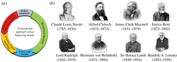
It is most common when first exposed to fluid dynamics and transport phenomena to learn and derive the conservation equations and then to solve the coupled equations for special cases where the spatio-temporal distribution of velocity, pressure and other scalar quantities of interest can be determined. In more advanced courses, and certainly in many applications, the equations may be solved numerically. It then follows that the tangential and normal stresses and scalar fluxes on a surface can be calculated so as to obtain forces and torques on, and heat and mass transfer from, objects. This standard approach focuses first on the detailed distribution of the primary variables and second on integrated quantities. Alternatively, the structure of the Navier–Stokes equations (or more generally the Cauchy stress equations of motion) and advection–diffusion–reaction equations provides a framework, at the outset, for describing integrated quantities, which at least in some cases allows bypassing some, if not all, of the details of the velocity, pressure, temperature or concentration fields. As sketched in figure 1(a), this focus on integrated quantities is the essence of the reciprocal theorem, which is the subject of this article.
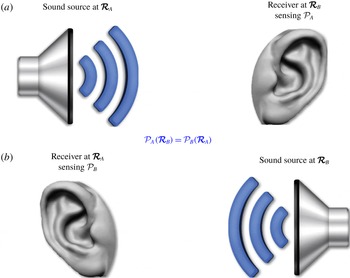
The reciprocal theorem offers a concise approach for understanding various integral properties of flows and transport processes. The technique is a relative of Green’s second identity, which is almost certainly familiar to all readers from introductory courses on partial differential equations. Indeed, for many readers the idea of ‘reciprocity’ is first encountered in acoustics, where the focus is on the scalar wave equation. Via Green’s second identity, we then learn that the response measured at location B due to an acoustic source at location A is the same as the response measured at A due to a source at B (see § 9). In this article, we present the way this ‘reciprocal’ idea arises in the two limits of low-Reynolds-number (i.e. Stokes) and inviscid flows, as well as common problems in heat and mass transfer. There is a large literature exploring various mathematical themes of the reciprocal theorem in related fields of elasticity, electromagnetism, etc. (see e.g. Achenbach Reference Achenbach, Schiavone, Constanda and Mioduchowski2002, Reference Achenbach2003, Reference Achenbach2014; Barber Reference Barber2002; Potton Reference Potton2004; Love Reference Love2013).
It might be surprising that the ‘reciprocal’ feature reviewed here – originally identified and often studied in dissipationless acoustic problems – is applicable to problems dominated by viscous effects. But, as we shall see, the key ideas to be explored are tied to the divergence form of the governing equations of fluid dynamics and transport phenomena; this mathematical structure is also highlighted in some numerical solutions. Indeed, already in 1953, Heaslet & Spreiter (Reference Heaslet and Spreiter1953) in an article in the aerodynamics literature wrote the following: ‘The generality in the statement of reciprocity relations appears, almost universally, to have held back their application to problems for which they are obviously, in retrospect, particularly fitted. This generality is even more apparent in some of the conclusions of Lord Rayleigh and von Helmholtz which apply to nonconservative systems’. This remark, made more than 65 years ago, appears to be equally true today.
(a) A diagram highlighting the advantage of using the reciprocal theorem versus following the conventional problem-solving approach for calculating integrated quantities, such as forces and torques in Stokes flows. Similar diagrams can be drawn for certain classes of inviscid flows and heat/mass transfer problems (see §§ 8–10). (b) Early contributors to the idea of the reciprocal theorem in physics and engineering. The portrait of Sir Horace Lamb is adapted, with permission, from National Portrait Gallery, London. The remaining photographs are adapted from Wikipedia.

1.1 History of the reciprocal theorem in continuum mechanics, electricity, magnetism and optics
The reciprocal theorem has been attributed to various famous figures in different fields of physics and engineering (see figure 1 b), though there is hardly a consensus on who was the founder. The earliest contribution, however, appears to have been made by the French engineer and physicist Navier (Reference Navier1826) in the context of statically indeterminate frame analysis (see Charlton Reference Charlton1960). The more developed version of the idea, in the same context, was later discussed by the German mathematician Clebsch (Reference Clebsch1862), who did not explicitly mention the phrase ‘reciprocal theorem’. Subsequent contributions were made by the Scottish physicist Maxwell (Reference Maxwell1864) and Italian mathematician Betti (Reference Betti1872). Maxwell (Reference Maxwell1881) also wrote about the reciprocal properties of two conductors in his book ‘A Treatise on Electricity and Magnetism’. Perhaps surprisingly, neither Navier nor Clebsch seem to have been credited properly in the elasticity literature, where the reciprocal theorem is most often attributed to Betti and sometimes to both Maxwell and Betti; the founding names are seldom mentioned in the fluid dynamics literature.
Betti’s work was later generalized by the British physicist and Nobel Prize winner Lord Rayleigh (Reference Rayleigh1873, Reference Rayleigh1876, Reference Rayleigh1877) and extended to the field of acoustics and sound generation. A reciprocal theorem was then developed by German physicist von Helmholtz (Reference von Helmholtz1887) for small variations in the momenta and coordinates of a general dynamical system in forward and reverse motion (Heaslet & Spreiter Reference Heaslet and Spreiter1953). An alternative derivation of the theorem was given by the British applied mathematician and fluid mechanician Lamb (Reference Lamb1887), whose work paved the way for establishing reverse-flow theorems in wing theory based on the inviscid flow limit (see Heaslet & Spreiter Reference Heaslet and Spreiter1953, and § 8). Along with the Irish physicist and mathematician Stokes (Reference Stokes1849), von Helmholtz (Reference von Helmholtz1856) is also credited for a reciprocity principle in optics, which in its most basic form states that ‘if I can see you, then you can see me’; the corresponding acoustic principle is, of course, ‘if I can hear you, then you can hear me’.
Finally, the version of the reciprocal theorem that appears in the low-Reynolds-number flow literature is attributed to the Dutch physicist and Nobel Prize winner Lorentz (Reference Lorentz1896). It appears that this contribution had been mainly overlooked by the fluid dynamics community until it was used by Brenner (Reference Brenner1958), who championed the application of the theorem throughout his career. According to Acrivos (Reference Acrivos2015), Brenner himself learned about Lorentz’s work while studying the book of the French fluid mechanician Villat (Reference Villat1943), which was lent to him by Brenner’s advisor John Happel; Brenner cited both Lorentz (Reference Lorentz1895) and Villat (Reference Villat1943) in the first paper where he used the reciprocal theorem (Brenner Reference Brenner1958). It is worth noting that Lorentz (Reference Lorentz1895) is also known for the reciprocity principle named after him in the field of electromagnetism.
1.2 Structure of this article
In this article, we explore various ways in which the reciprocal theorem gives insights into fluid dynamics problems as well as problems in heat and mass transfer, including the influence of convection. In particular, we will see that the theorem for low-Reynolds-number flows, or its equivalent idea for high-Reynolds-number inviscid flows, provides a means to
(i) derive integral equation representations for the velocity distribution, which are often useful as an approach to numerical simulations;
(ii) learn about various symmetries of tensorial properties of a flow;
(iii) understand some of the features of particle shape, Reynolds number, wall slip, etc. on forces and torques on particles or the self-propulsion of particles;
(iv) study the flow rate, or other related integral quantities, in channel flows with a specified slip velocity distribution;
(v) determine the lift coefficient for an arbitrarily cambered thin airfoil;
(vi) describe various mathematical features of acoustics and the relation of sound propagation and reception between a source and a receiver; and
(vii) describe quantitatively the effect of non-uniform boundary conditions and particle shape on problems of heat and mass transfer.
It is occasionally remarked that solutions obtained with the reciprocal theorem appear almost miraculously using limited information, other than the statement of the boundary-value problem. Thus, it may seem like ‘one gets something for nothing’. We shall try to illustrate the ideas in § 2 with a few standard boundary-value problems, prior to turning in § 3 to the structure of the reciprocal theorem as it is commonly developed in low-Reynolds-number hydrodynamics, e.g. for arriving at integral equation representations of the velocity field (§ 4). Next, the theorem is applied to externally and self-driven particle motions (§§ 5 and 6, respectively) and to a channel flow (§ 7). Proceeding beyond the realm of viscously dominated flows, in the following sections, we utilize the ideas discussed in § 2 to formulate reciprocal relations that serve as shortcut solutions to exemplary problems in high-Reynolds-number inviscid flows (§ 8), acoustics (§ 9) and convective heat/mass transfer (§ 10). Finally, we provide a brief overview and concluding remarks in § 11. Throughout the text, we provide many references, but recognize that inevitable limitations of this kind of article do not let us list every relevant paper (not that we are even aware of all possible contributions to this literature).
Readers may also be interested to study Onsager reciprocal relations (Onsager Reference Onsager1931a ,Reference Onsager b ) and the principle of virtual work (Howell Reference Howell2001), both of which are known to provide ‘something for nothing’. The former establish the equality of particular ratios between generalized forces and generalized fluxes in irreversible thermodynamic processes and lead to many important conclusions without a need for conducting detailed field calculations. The latter is a hallmark of theoretical solid mechanics, which shares many mathematical similarities with, and so functions analogous to, the reciprocal theorem discussed here.
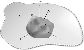
Schematic of an arbitrarily shaped particle, with surface
 $S_{p}$
and unit outward normal vector
 $\boldsymbol{n}$
, in an unbounded fluid domain. The dashed line indicates an enclosing boundary in the ‘far field’.

2 Pedagogy
There are a number of mathematical facts that are needed to appreciate the development and use of the reciprocal theorem. Some of the mathematical statements are so common that most practitioners are not aware of how useful the results can be for obtaining more detailed insights or even solutions to specific applied mathematics, fluid dynamics or transport phenomena problems. In this first mathematical section, we develop a few of the ideas common to the typical steps in applying the reciprocal theorem for problems described by the scalar Helmholtz and Laplace equations (§ 2.1). We also introduce the way perturbation expansions are used with the reciprocal theorem, including examples where the perturbation is in the shape of the boundary (§ 2.2.1) and in a nonlinear term present in the governing equation (§ 2.2.2). In later examples in this paper, the ideas introduced in this section will be used.
Throughout much of the discussion below, we consider a particle with surface
 $S_{p}$
immersed in a fluid domain
 $V$
(see figure 2), and denote as
 $\boldsymbol{n}$
the unit normal vector directed into the fluid. In many cases, we explicitly recognize a bounding surface at large distances
 $S_{\infty }$
and represent the position vector and its magnitude by
 $\boldsymbol{r}$
and
 $r=|\boldsymbol{r}|$
, respectively.
2.1 Green’s second identity and getting something for nothing
Consider solving a (dimensionless) steady-state reaction–diffusion problem outside of an arbitrarily shaped particle, where the concentration is denoted
 $\unicode[STIX]{x1D713}(\boldsymbol{r})$
; the medium is at rest. Suppose that there are specified surface values for the function
 $\unicode[STIX]{x1D713}$
and assume that
 $\unicode[STIX]{x1D713}$
vanishes at infinity. The boundary-value problem is
 $$\begin{eqnarray}\unicode[STIX]{x1D6FB}^{2}\unicode[STIX]{x1D713}=\unicode[STIX]{x1D6FC}^{2}\unicode[STIX]{x1D713},\quad \text{with }\unicode[STIX]{x1D713}(\boldsymbol{r})=g(\boldsymbol{r})\text{ for }\boldsymbol{r}\in S_{p}\text{ and }\unicode[STIX]{x1D713}\rightarrow 0\text{ as }r\rightarrow \infty ,\end{eqnarray}$$
where
 $\unicode[STIX]{x1D6FC}$
is a constant; in practice
 $\unicode[STIX]{x1D6FC}^{2}=\unicode[STIX]{x1D55C}_{r}\ell ^{2}/D$
, where
 $\unicode[STIX]{x1D55C}_{r}$
is a rate constant for a first-order chemical reaction,
 $\ell$
is a characteristic geometric length scale and
 $D$
is the diffusion constant. Here,
 $g(\boldsymbol{r})$
is a given function defined on the surface
 $S_{p}$
of the particle. Obviously, we might be interested in the detailed distribution of the scalar field
 $\unicode[STIX]{x1D713}(\boldsymbol{r})$
, but, in many cases, all we really want to know is the total flux
 $Q$
from the sphere,
 $$\begin{eqnarray}Q=-\int _{S_{p}}\boldsymbol{n}\boldsymbol{\cdot }\unicode[STIX]{x1D735}\unicode[STIX]{x1D713}\,\text{d}S=\int _{S_{p}}q\,\text{d}S,\end{eqnarray}$$
and how the given surface distribution
 $g(\boldsymbol{r})$
influences
 $Q$
; here, we have introduced
 $q=-\boldsymbol{n}\boldsymbol{\cdot }\unicode[STIX]{x1D735}\unicode[STIX]{x1D713}$
as the local flux. We now show how to deduce the integrated flux
 $Q$
without explicitly solving for
 $\unicode[STIX]{x1D713}(\boldsymbol{r})$
. It is worth noting that in the mass transfer literature, the dimensionless total mass transfer rate is represented by the Sherwood number
 $Sh$
.
To start, we consider a problem whose solution we assume that we know (analytically or numerically), which, in this case, is the solution to the Helmholtz equation for a particle with uniform surface values. So, consider
 $$\begin{eqnarray}\unicode[STIX]{x1D6FB}^{2}\hat{\unicode[STIX]{x1D713}}=\unicode[STIX]{x1D6FC}^{2}\hat{\unicode[STIX]{x1D713}},\quad \text{with }\hat{\unicode[STIX]{x1D713}}(\boldsymbol{r})=1\text{ for }\boldsymbol{r}\in S_{p}\text{ and }\hat{\unicode[STIX]{x1D713}}\rightarrow 0\text{ as }r\rightarrow \infty .\end{eqnarray}$$
Second, we derive a general mathematical identify, which proves to be an important starting point for subsequent steps and applies generally, independent of the boundary shape. This theorem is established by multiplying the Helmholtz equation in (2.1) by
 $\hat{\unicode[STIX]{x1D713}}(r)$
and the one in (2.3) by
 $\unicode[STIX]{x1D713}$
, and then subtracting to obtain
 $$\begin{eqnarray}\hat{\unicode[STIX]{x1D713}}\unicode[STIX]{x1D6FB}^{2}\unicode[STIX]{x1D713}-\unicode[STIX]{x1D713}\unicode[STIX]{x1D6FB}^{2}\hat{\unicode[STIX]{x1D713}}=0.\end{eqnarray}$$
Next, note the vector identity that
 $\unicode[STIX]{x1D735}\boldsymbol{\cdot }(\hat{\unicode[STIX]{x1D713}}\unicode[STIX]{x1D735}\unicode[STIX]{x1D713})=\hat{\unicode[STIX]{x1D713}}\unicode[STIX]{x1D6FB}^{2}\unicode[STIX]{x1D713}-\unicode[STIX]{x1D735}\hat{\unicode[STIX]{x1D713}}\boldsymbol{\cdot }\unicode[STIX]{x1D735}\unicode[STIX]{x1D713}$
; a similar equation can be written interchanging
 $\unicode[STIX]{x1D713}$
and
 $\hat{\unicode[STIX]{x1D713}}$
. Thus, equation (2.4) simplifies to
 $$\begin{eqnarray}\unicode[STIX]{x1D735}\boldsymbol{\cdot }\left(\hat{\unicode[STIX]{x1D713}}\unicode[STIX]{x1D735}\unicode[STIX]{x1D713}\right)=\unicode[STIX]{x1D735}\boldsymbol{\cdot }\left(\unicode[STIX]{x1D713}\unicode[STIX]{x1D735}\hat{\unicode[STIX]{x1D713}}\right).\end{eqnarray}$$
Integrating this equation over the domain external to the particle and using the divergence theorem, we obtain
 $$\begin{eqnarray}\int _{S}\hat{\unicode[STIX]{x1D713}}\,\boldsymbol{n}\boldsymbol{\cdot }\unicode[STIX]{x1D735}\unicode[STIX]{x1D713}\,\text{d}S=\int _{S}\unicode[STIX]{x1D713}\,\boldsymbol{n}\boldsymbol{\cdot }\unicode[STIX]{x1D735}\hat{\unicode[STIX]{x1D713}}\,\text{d}S,\end{eqnarray}$$
where
 $S$
denotes all the surfaces bounding the fluid domain
 $V$
, i.e.
 $S=S_{p}+S_{\infty }$
(see figure 2). The result (2.6) is known as Green’s second identity and is the scalar equivalent of the reciprocal theorem (equation (3.12) of the next section), which proves to be so useful in fluid dynamics and transport phenomenon as this article tries to demonstrate.
Now, we are in a position to answer our original question, which is to obtain the integrated flux
 $Q$
for the boundary-value problem (2.1). We substitute into (2.6) the boundary conditions from (2.1) and (2.3) – note that the contributions from
 $S_{\infty }$
vanish – and so find
 $$\begin{eqnarray}\int _{S_{p}}q\,\text{d}S=Q=\int _{S_{p}}g(\boldsymbol{r})\;\hat{q}\,\text{d}S.\end{eqnarray}$$
If we have previously determined
 $\hat{\unicode[STIX]{x1D713}}$
, either analytically or numerically, then
 $\hat{q}$
is known, and it only remains to integrate a known function for the given surface distribution
 $g(\boldsymbol{r})$
(the right-hand side of (2.7)) to obtain the total flux
 $Q$
. In particular, we have not had to determine the detailed distribution
 $\unicode[STIX]{x1D713}(\boldsymbol{r})$
for the given
 $g(\boldsymbol{r})$
, which was the original boundary-value problem, equation (2.1). It is as if we have gotten something – the integrated flux
 $Q$
– for nothing, since we only have to integrate the given boundary data on the right-hand side of (2.7)!
In the special case of a spherical particle of unit radius, the model problem (2.3) has the solution
 $\hat{\unicode[STIX]{x1D713}}(r)=r^{-1}\text{e}^{\unicode[STIX]{x1D6FC}(1-r)}$
, where
 $r$
is the radial distance from the centre of the sphere. Therefore, the flux at the surface of the sphere
 $(r=1)$
is
 $\hat{q}=-\boldsymbol{n}\boldsymbol{\cdot }\unicode[STIX]{x1D735}\hat{\unicode[STIX]{x1D713}}=-\text{d}\hat{\unicode[STIX]{x1D713}}/\text{d}r=1+\unicode[STIX]{x1D6FC}$
. Hence, we have
 $$\begin{eqnarray}Q=\left(1+\unicode[STIX]{x1D6FC}\right)\int _{S_{p}}g(\boldsymbol{r})\,\text{d}S,\end{eqnarray}$$
which indicates that we only need to integrate the given surface function
 $g(\boldsymbol{r})$
to obtain
 $Q$
.
2.2 Perturbation expansions
We next illustrate how Green’s second identity can be used to construct other solutions to problems involving differential equations, at least when an integrated quantity is desired, for those cases involving a (small) parameter, which we shall denote
 $\unicode[STIX]{x1D700}$
. Readers will be familiar with perturbation expansions, e.g. Hinch (Reference Hinch1991). A problem can be perturbed in the form of the governing equation, in the form of the boundary conditions, or in the shape of the boundary. We now consider two examples to make the basic steps and ideas clear, as these kinds of examples will arise later in the article and find a variety of applications in research.
2.2.1 An example with a perturbation expansion: using Taylor series for handling the boundary condition on a complicated shape
As an example of a problem where the shape of a boundary is perturbed, consider solving the Laplace or Helmholtz equation outside of a nearly spherical shape or inside a square or cylinder with rough boundaries, which could be taken as a periodic perturbation. The approach to such problems that we use is generally called ‘domain perturbation’ in the literature (e.g. Joseph Reference Joseph1973) and it comes up in a variety of examples in fluid dynamics and transport phenomena.
In the specific example we discuss here, it is convenient to use spherical coordinates
 $(r,\unicode[STIX]{x1D703},\unicode[STIX]{x1D711})$
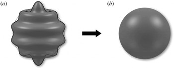
and we treat the Laplace equation outside of a nearly spherical shape, i.e. a ‘near sphere’ (see figure 3). Also, the mean radius is unity and the shape is denoted by the perturbation parameter
 $\unicode[STIX]{x1D700}$
times a shape function
 $h(\unicode[STIX]{x1D703},\unicode[STIX]{x1D719})$
. We consider
 $$\begin{eqnarray}\unicode[STIX]{x1D6FB}^{2}\unicode[STIX]{x1D713}=0,\quad \text{with }\unicode[STIX]{x1D713}=1\text{ at }r=1+\unicode[STIX]{x1D700}h(\unicode[STIX]{x1D703},\unicode[STIX]{x1D713})\text{ and }\unicode[STIX]{x1D713}\rightarrow 0\text{ as }r\rightarrow \infty ,\end{eqnarray}$$
where
 $0<|\unicode[STIX]{x1D700}|\ll 1$
. The novelty here is the presence of the non-spherical shape specified by
 $h(\unicode[STIX]{x1D703},\unicode[STIX]{x1D711})$
. We can imagine seeking the detailed solution
 $\unicode[STIX]{x1D713}(r,\unicode[STIX]{x1D703},\unicode[STIX]{x1D711};\unicode[STIX]{x1D700})$
to (2.9) or perhaps we are most interested in how the surface flux integrated over the surface
 $S_{p}$
depends on the shape perturbation, i.e.
 $Q=\int _{S_{p}}q\,\text{d}S$
for a given
 $h(\unicode[STIX]{x1D703},\unicode[STIX]{x1D711})$
. We now show how to obtain
 $Q$
to
 $O(\unicode[STIX]{x1D700})$
without explicitly determining
 $\unicode[STIX]{x1D713}$
to
 $O(\unicode[STIX]{x1D700})$
.
Boundary conditions on the surface of a ‘near sphere’ (a) can be mapped to the boundary of the unperturbed sphere (b) using a Taylor series expansion.

Since
 $0<|\unicode[STIX]{x1D700}|\ll 1$
, we pose a perturbation expansion as
 $$\begin{eqnarray}\unicode[STIX]{x1D713}=\unicode[STIX]{x1D713}^{(0)}+\unicode[STIX]{x1D700}\unicode[STIX]{x1D713}^{(1)}+O(\unicode[STIX]{x1D700}^{2}).\end{eqnarray}$$
Clearly, from (2.9), at each order  of the expansion, we observe that
 . What about the boundary conditions?
We use a Taylor series expansion of the function
 $\unicode[STIX]{x1D713}(\boldsymbol{r})$
about the spherical shape
 $r=1$
, apply the boundary condition (2.9) on the surface, and also use the perturbation expansion (2.10) to arrive at
 $$\begin{eqnarray}\displaystyle & & \displaystyle \unicode[STIX]{x1D713}\left(r=1+\unicode[STIX]{x1D700}h(\unicode[STIX]{x1D703},\unicode[STIX]{x1D711}),\unicode[STIX]{x1D703},\unicode[STIX]{x1D711}\right)\nonumber\\ \displaystyle & & \displaystyle \quad =\unicode[STIX]{x1D713}^{(0)}(1,\unicode[STIX]{x1D703},\unicode[STIX]{x1D711})\end{eqnarray}$$
 $$\begin{eqnarray}\displaystyle & & \displaystyle \qquad +\,\unicode[STIX]{x1D700}\left[\unicode[STIX]{x1D713}^{(1)}(1,\unicode[STIX]{x1D703},\unicode[STIX]{x1D711})+h(\unicode[STIX]{x1D703},\unicode[STIX]{x1D711})\left.\frac{\unicode[STIX]{x2202}\unicode[STIX]{x1D713}^{(0)}}{\unicode[STIX]{x2202}r}\right|_{r=1}\right]+O(\unicode[STIX]{x1D700}^{2})=1.\end{eqnarray}$$
 $\unicode[STIX]{x1D700}$
, we arrive at the boundary conditions
 $$\begin{eqnarray}\unicode[STIX]{x1D713}^{(0)}(1,\unicode[STIX]{x1D703},\unicode[STIX]{x1D711})=1\quad \text{and}\quad \unicode[STIX]{x1D713}^{(1)}(1,\unicode[STIX]{x1D703},\unicode[STIX]{x1D711})=-h(\unicode[STIX]{x1D703},\unicode[STIX]{x1D711})\left.\frac{\unicode[STIX]{x2202}\unicode[STIX]{x1D713}^{(0)}}{\unicode[STIX]{x2202}r}\right|_{r=1}.\end{eqnarray}$$
These steps of domain perturbation have effectively mapped the original boundary-value problem to a spherical surface
 $(r=1)$
, which we denote
 $S_{0}$
. An interested reader may wish to carry out these steps to the next order in
 $\unicode[STIX]{x1D700}$
.
Of course, we can proceed to construct the detailed solutions for the functions  ,but suppose we are most interested in the integrated surface flux
 $Q=\int _{S_{p}}q\,\text{d}S$
, where, as before,
 $q=-\boldsymbol{n}\boldsymbol{\cdot }\unicode[STIX]{x1D735}\unicode[STIX]{x1D713}$
. Substituting for
 $\unicode[STIX]{x1D713}$
and realizing that

(as  everywhere including in the volume enclosed between
 $S_{0}$
and
 $S_{p}$
), we can write
 $Q=Q^{(0)}+\unicode[STIX]{x1D700}\,Q^{(1)}+O(\unicode[STIX]{x1D700}^{2})$
, where
 and, for example,
 $q^{(0)}=-\text{d}\unicode[STIX]{x1D713}^{(0)}/\text{d}r$
. Since an analytical solution is known for the axisymmetric case
 $\unicode[STIX]{x1D713}^{(0)}(r)$
, then we know by direct calculation
 $\unicode[STIX]{x1D713}^{(0)}=r^{-1}$
,
 $\text{d}\unicode[STIX]{x1D713}^{(0)}/\text{d}r|_{r=1}=-1$
, and
 $Q^{(0)}=4\unicode[STIX]{x03C0}$
(see § 2.1 with
 $\unicode[STIX]{x1D6FC}=0$
).
The
 $O(\unicode[STIX]{x1D700})$
flux
 $Q^{(1)}$
can, in fact, be obtained by using Green’s second identity, as it was presented in (2.6). We identify the two field variables to consider as
 $\unicode[STIX]{x1D713}^{(0)}$
and
 $\unicode[STIX]{x1D713}^{(1)}$
, as both are solutions to the Laplace equation defined now on a spherical surface
 $S_{0}$
, but each satisfies different boundary conditions, as given in (2.12). Thus, beginning with (2.6), we use the appropriate boundary conditions (2.12) and discover
 $$\begin{eqnarray}\displaystyle \int _{S_{0}}\unicode[STIX]{x1D713}^{(0)}q^{(1)}\,\text{d}S & = & \displaystyle \int _{S_{0}}\unicode[STIX]{x1D713}^{(1)}q^{(0)}\,\text{d}S,\end{eqnarray}$$
 $$\begin{eqnarray}\displaystyle \Rightarrow \quad Q^{(1)} & = & \displaystyle \int _{S_{0}}h(\unicode[STIX]{x1D703},\unicode[STIX]{x1D711})\left(\left.\frac{\text{d}\unicode[STIX]{x1D713}^{(0)}}{\text{d}r}\right|_{r=1}\right)^{2}\text{d}S=\int _{S_{0}}h(\unicode[STIX]{x1D703},\unicode[STIX]{x1D711})\,\text{d}S.\end{eqnarray}$$
 $O(\unicode[STIX]{x1D700})$
contribution to the total surface flux as an integral of the given function
 $h(\unicode[STIX]{x1D703},\unicode[STIX]{x1D711})$
. Therefore, the integrated surface flux is
 $$\begin{eqnarray}Q=4\unicode[STIX]{x03C0}+\unicode[STIX]{x1D700}\int _{S}h(\unicode[STIX]{x1D703},\unicode[STIX]{x1D711})\,\text{d}S+O(\unicode[STIX]{x1D700}^{2}).\end{eqnarray}$$
However, in reaching this result we never had to obtain the corresponding
 $O(\unicode[STIX]{x1D700})$
field
 $\unicode[STIX]{x1D713}^{(1)}(\boldsymbol{r})$
. The approach demonstrated here and the explicit result, equation (2.15), is the miracle of the reciprocal theorem in that, with the known textbook solution for
 $\unicode[STIX]{x1D713}^{(0)}(r)$
, we have calculated the
 $O(\unicode[STIX]{x1D700})$
correction to the total flux; again, we suggest that we have gotten something for nothing.
2.2.2 An example with a perturbation expansion: linearizing the governing equation
As an example of a nonlinear differential equation that can be tackled, at least approximately, using the reciprocal theorem, we consider spherical coordinates for the domain outside a sphere of unit radius and take the problem statement
 $$\begin{eqnarray}\unicode[STIX]{x1D6FB}^{2}\unicode[STIX]{x1D713}=\unicode[STIX]{x1D700}\unicode[STIX]{x1D713}^{3},\quad \text{with }\unicode[STIX]{x1D713}=1\text{ on }r=1\text{ and }\unicode[STIX]{x1D713}\rightarrow 0\text{ as }r\rightarrow \infty .\end{eqnarray}$$
For the simple axisymmetric boundary conditions here, the problem is that of an ordinary differential equation. We continue to assume
 $\unicode[STIX]{x1D700}\ll 1$
. This example has been chosen for illustrative purposes, but we can notice that the appearance of the
 $O(\unicode[STIX]{x1D700})$
terms on the right-hand side is conceptually similar to considering corrections to the diffusion equation due to a concentration dependent diffusivity or inertial corrections to the Stokes limit of the Navier–Stokes equations.
Although we can seek to construct
 $\unicode[STIX]{x1D713}(\boldsymbol{r};\unicode[STIX]{x1D700})$
(indeed it is straightforward to do so using a regular perturbation expansion), we may only be interested in the integrated flux
 $$\begin{eqnarray}Q=\int _{S_{p}}q\,\text{d}S=-\int _{S_{p}}\frac{\unicode[STIX]{x2202}\unicode[STIX]{x1D713}}{\unicode[STIX]{x2202}r}\,\text{d}S.\end{eqnarray}$$
Again, we begin with a regular perturbation expansion (2.10), which leads to a sequence of boundary-value problems,
 $$\begin{eqnarray}\displaystyle & \displaystyle \unicode[STIX]{x1D6FB}^{2}\unicode[STIX]{x1D713}^{(0)}=0\quad \text{with }\unicode[STIX]{x1D713}^{(0)}(1)=1\text{ and }\unicode[STIX]{x1D713}^{(0)}(\infty )\rightarrow 0, & \displaystyle\end{eqnarray}$$
 $$\begin{eqnarray}\displaystyle & \displaystyle \unicode[STIX]{x1D6FB}^{2}\unicode[STIX]{x1D713}^{(1)}=\left(\unicode[STIX]{x1D713}^{(0)}\right)^{3}\quad \text{with }\unicode[STIX]{x1D713}^{(1)}(1)=0\text{ and }\unicode[STIX]{x1D713}^{(1)}(\infty )\rightarrow 0, & \displaystyle\end{eqnarray}$$
 $$\begin{eqnarray}\displaystyle & \displaystyle \unicode[STIX]{x1D6FB}^{2}\unicode[STIX]{x1D713}^{(2)}=3\left(\unicode[STIX]{x1D713}^{(0)}\right)^{2}\unicode[STIX]{x1D713}^{(1)}\quad \text{with }\unicode[STIX]{x1D713}^{(2)}(1)=0\text{ and }\unicode[STIX]{x1D713}^{(2)}(\infty )\rightarrow 0. & \displaystyle\end{eqnarray}$$
 $Q=Q^{(0)}+\unicode[STIX]{x1D700}\,Q^{(1)}+\unicode[STIX]{x1D700}^{2}Q^{(2)}+O(\unicode[STIX]{x1D700}^{3})$
, where we have already seen that
 $Q^{(0)}=4\unicode[STIX]{x03C0}$
. The
 $O(\unicode[STIX]{x1D700})$
correction requires that we calculate
 $Q^{(1)}=-\int _{S_{p}}\unicode[STIX]{x2202}\unicode[STIX]{x1D713}^{(1)}/\unicode[STIX]{x2202}r\,\text{d}S$
. To obtain this integral, we use (2.18a
) and (2.18b
) and carry out the steps familiar from Green’s second identity, as in § 2.1. Accounting for the right-hand side in (2.18b
) and for the sign convention in the divergence theorem, we arrive at
 $$\begin{eqnarray}\int _{S_{p}}\unicode[STIX]{x1D713}^{(0)}q^{(1)}\,\text{d}S-\int _{S_{p}}\unicode[STIX]{x1D713}^{(1)}q^{(0)}\,\text{d}S=\int _{V}\left(\unicode[STIX]{x1D713}^{(0)}\right)^{4}\text{d}V.\end{eqnarray}$$
The volume integral on the right-hand side is the new feature. Applying the boundary conditions and recalling
 $\unicode[STIX]{x1D713}^{(0)}(r)=1/r$
gives
 $$\begin{eqnarray}Q^{(1)}=\int _{S_{p}}q^{(1)}\,\text{d}S=\int _{V}r^{-4}\,\text{d}V=4\unicode[STIX]{x03C0}\int _{1}^{\infty }r^{-2}\,\text{d}r=4\unicode[STIX]{x03C0}.\end{eqnarray}$$
One can immediately proceed to calculate the next term in the total flux
 $Q^{(2)}=-\!\int _{S_{p}}\unicode[STIX]{x2202}\unicode[STIX]{x1D713}^{(2)}/\unicode[STIX]{x2202}r\,\text{d}S$
, by utilizing (2.18a
) and (2.18c
), to find
 $$\begin{eqnarray}\int _{S_{p}}\unicode[STIX]{x1D713}^{(0)}q^{(2)}\,\text{d}S-\int _{S_{p}}\unicode[STIX]{x1D713}^{(2)}q^{(0)}\,\text{d}S=3\int _{V}\unicode[STIX]{x1D713}^{(1)}\left(\unicode[STIX]{x1D713}^{(0)}\right)^{3}\text{d}S.\end{eqnarray}$$
Here, we need
 $\unicode[STIX]{x1D713}^{(1)}(r)$
, which emphasizes that the reciprocal theorem approach generally produces an integrated quantity to one order higher in
 $\unicode[STIX]{x1D700}$
than the corresponding field that is known. In this case,
 $\unicode[STIX]{x1D713}^{(1)}(r)=-r^{-1}\ln r$
as shown by a direct calculation, and so utilizing the boundary conditions, we find
 $$\begin{eqnarray}Q^{(2)}=\int _{S_{p}}q^{(2)}\,\text{d}S=3\int _{V}\left(\unicode[STIX]{x1D713}^{(0)}\right)^{3}\unicode[STIX]{x1D713}^{(1)}\,\text{d}S=-3\times 4\unicode[STIX]{x03C0}\int _{1}^{\infty }r^{-2}\ln r\,\text{d}r=-12\unicode[STIX]{x03C0}.\end{eqnarray}$$
We have thus established
 $Q=4\unicode[STIX]{x03C0}[1+\unicode[STIX]{x1D700}-3\unicode[STIX]{x1D700}^{2}+O(\unicode[STIX]{x1D700}^{3})]$
. It is straightforward to continue to higher orders.
Note that similar ideas apply if the original problem statement involved a spatially dependent boundary condition, e.g.
 $\unicode[STIX]{x1D713}(\boldsymbol{r})=g(\unicode[STIX]{x1D703},\unicode[STIX]{x1D711})$
on
 $r=1$
, in which case one has to solve a partial differential equation. We found in § 2.1 that
 $Q^{(0)}=\int _{S_{p}}g(\unicode[STIX]{x1D703},\unicode[STIX]{x1D711})\,\text{d}S$
can be calculated by straightforward integration. At the next order, we use (2.18b
) for
 $\unicode[STIX]{x1D713}^{(1)}$
and construct the reciprocal theorem using the fundamental solution
 $\hat{\unicode[STIX]{x1D713}}=1/r$
, which leads to an equation similar to (2.19),
 $$\begin{eqnarray}\int _{S_{p}}\hat{\unicode[STIX]{x1D713}}\,q^{(1)}\,\text{d}S-\int _{S_{p}}\unicode[STIX]{x1D713}^{(1)}\,\hat{q}\,\text{d}S=\int _{V}\hat{\unicode[STIX]{x1D713}}\left(\unicode[STIX]{x1D713}^{(0)}\right)^{3}\text{d}V.\end{eqnarray}$$
Thus, we conclude that
 $$\begin{eqnarray}Q^{(1)}=\int _{V}r^{-1}\left(\unicode[STIX]{x1D713}^{(0)}\right)^{3}\text{d}V.\end{eqnarray}$$
If
 $\unicode[STIX]{x1D713}^{(0)}(r,\unicode[STIX]{x1D703},\unicode[STIX]{x1D711})$
is known in terms of an eigenfunction expansion, then, in principle, the integral is straightforward to calculate using the orthogonality of the eigenfunctions.
3 Low-Reynolds-number flows and the reciprocal theorem
We now turn our attention to low-Reynolds-number fluid motions, which are characteristic of a diverse range of phenomena, spanning biology, engineering and material science, among other fields. We identify the Reynolds number as
 $Re=\unicode[STIX]{x1D70C}U\ell /\unicode[STIX]{x1D707}$
, where
 $\unicode[STIX]{x1D70C}$
is the fluid density,
 $\unicode[STIX]{x1D707}$
is the fluid viscosity,
 $\ell$
is a typical (usually geometric) length scale and
 $U$
is a typical scale for the velocity; as is well known, this ratio approximates the relative magnitude of the inertial terms to the viscous terms in the Navier–Stokes equations, which are introduced below. The limit
 $Re\ll 1$
is representative of many ‘small-scale’ flows where the length scale is small, e.g. this is common to biological flows at the scale of the cell and colloid science where sizes are tens of microns and smaller. Similarly, motions with very large viscosities have
 $Re\ll 1$
and so are common in geophysics, e.g. lava flows and motions in the Earth’s mantle. In addition, flows in the subsurface of the Earth constitute an important example of flow in porous media, and generally are described by
 $Re\ll 1$
since the pore-scale dimensions are small and/or the viscosity is large (e.g. crude oils). Building upon the ideas presented in the previous section, here, we derive the general form of the reciprocal theorem for low-
 $Re$
flows, and apply it to obtain (as a general result) integral equation representations of the solution to the Stokes equations for two types of flows, one single and the other two phase.
3.1 The equations of motion
To start our discussion of fluid dynamics, we denote the velocity field
 $\boldsymbol{u}$
, the pressure
 $p$
, the (symmetric) stress tensor
 $\unicode[STIX]{x1D748}$
and the body force per unit volume
 $\boldsymbol{b}$
, and recall the continuity equation and the Cauchy stress equations of motions for an incompressible flow
 $$\begin{eqnarray}\unicode[STIX]{x1D70C}\left(\frac{\unicode[STIX]{x2202}\boldsymbol{u}}{\unicode[STIX]{x2202}t}+\boldsymbol{u}\boldsymbol{\cdot }\unicode[STIX]{x1D735}\boldsymbol{u}\right)=\unicode[STIX]{x1D735}\boldsymbol{\cdot }\unicode[STIX]{x1D748}+\boldsymbol{b}\quad \text{and}\quad \unicode[STIX]{x1D735}\boldsymbol{\cdot }\boldsymbol{u}=0.\end{eqnarray}$$
For many common and important problems, the fluid is Newtonian, meaning
 $$\begin{eqnarray}\unicode[STIX]{x1D748}=-p\unicode[STIX]{x1D644}+2\unicode[STIX]{x1D707}\unicode[STIX]{x1D640},\quad \text{with }\unicode[STIX]{x1D640}={\textstyle \frac{1}{2}}\left[\unicode[STIX]{x1D735}\boldsymbol{u}+\left(\unicode[STIX]{x1D735}\boldsymbol{u}\right)^{\text{T}}\right],\end{eqnarray}$$
where
 $\unicode[STIX]{x1D644}$
is the identity tensor and
 $\unicode[STIX]{x1D640}$
is the rate of strain tensor (which is symmetric). Thus, we see that we can write the Navier–Stokes and continuity equations (3.1) for a fluid of constant viscosity and density as
 $$\begin{eqnarray}\unicode[STIX]{x1D70C}\left(\frac{\unicode[STIX]{x2202}\boldsymbol{u}}{\unicode[STIX]{x2202}t}+\boldsymbol{u}\boldsymbol{\cdot }\unicode[STIX]{x1D735}\boldsymbol{u}\right)=-\unicode[STIX]{x1D735}p+\unicode[STIX]{x1D707}\unicode[STIX]{x1D6FB}^{2}\boldsymbol{u}+\boldsymbol{b}=\unicode[STIX]{x1D735}\boldsymbol{\cdot }\unicode[STIX]{x1D748}+\boldsymbol{b}\quad \text{and}\quad \unicode[STIX]{x1D735}\boldsymbol{\cdot }\boldsymbol{u}=0.\end{eqnarray}$$
The common low-Reynolds-number flow assumption leads to the neglect of the inertial terms, in which case we have the Stokes equations
 $$\begin{eqnarray}-\unicode[STIX]{x1D735}p+\unicode[STIX]{x1D707}\unicode[STIX]{x1D6FB}^{2}\boldsymbol{u}+\boldsymbol{b}=\unicode[STIX]{x1D735}\boldsymbol{\cdot }\unicode[STIX]{x1D748}+\boldsymbol{b}=\mathbf{0}\quad \text{and}\quad \unicode[STIX]{x1D735}\boldsymbol{\cdot }\boldsymbol{u}=0.\end{eqnarray}$$
For the problem solving discussed below, we most often think about the equations in the form
 $\unicode[STIX]{x1D735}\boldsymbol{\cdot }\unicode[STIX]{x1D748}+\boldsymbol{b}=\mathbf{0}$
, which is a form suitable for the reciprocal theorem.
If we incorporate the inertial terms from the Navier–Stokes equations on the left-hand side of the first equation of (3.3) with the body force terms, we can define an effective body force  , where
 depends on
 $\boldsymbol{u}$
and its spatial and time derivatives, and so also depends on the Reynolds number. Then, we can think of the Navier–Stokes equations in a similar form

In the following steps, we take advantage of this ‘divergence’ structure of the equations of motion.
3.2 The reciprocal theorem for the Stokes flow of a Newtonian fluid
Our interest is to solve
 $$\begin{eqnarray}\unicode[STIX]{x1D735}\boldsymbol{\cdot }\unicode[STIX]{x1D748}+\boldsymbol{b}=\mathbf{0}\quad \text{and}\quad \unicode[STIX]{x1D735}\boldsymbol{\cdot }\boldsymbol{u}=0\end{eqnarray}$$
for a wide range of different problems to be illustrated in this and subsequent sections, each of which is typically distinguished by different boundary conditions on the bounding surfaces
 $S$
. As we shall see later, by ‘solve’ we typically mean to determine some integrated quantity of interest, such as a force or torque. It is convenient to consider a ‘model’ problem with the same boundaries
 $S$
for which we suppose that we know the solution
 $(\hat{\boldsymbol{u}},\hat{\unicode[STIX]{x1D748}})$
satisfying
 $$\begin{eqnarray}\unicode[STIX]{x1D735}\boldsymbol{\cdot }\hat{\unicode[STIX]{x1D748}}+\hat{\boldsymbol{b}}=\mathbf{0}\quad \text{and}\quad \unicode[STIX]{x1D735}\boldsymbol{\cdot }\hat{\boldsymbol{u}}=0.\end{eqnarray}$$
This model problem takes various forms, e.g. flow past a sphere for which an explicit solution is available or the solution for a point force, depending on the original problem under consideration.
Next, we follow the basic steps that are used to construct Green’s second identity in § 2. Take the inner product of
 $\hat{\boldsymbol{u}}$
with (3.6) and subtract the inner product of
 $\boldsymbol{u}$
with (3.7),
 $$\begin{eqnarray}\left(\unicode[STIX]{x1D735}\boldsymbol{\cdot }\unicode[STIX]{x1D748}\right)\boldsymbol{\cdot }\hat{\boldsymbol{u}}-\left(\unicode[STIX]{x1D735}\boldsymbol{\cdot }\hat{\unicode[STIX]{x1D748}}\right)\boldsymbol{\cdot }\boldsymbol{u}=\boldsymbol{u}\boldsymbol{\cdot }\hat{\boldsymbol{b}}-\hat{\boldsymbol{u}}\boldsymbol{\cdot }\boldsymbol{b}.\end{eqnarray}$$
Consider one of the terms on the left-hand side, for example, the first term
 $$\begin{eqnarray}\left(\unicode[STIX]{x1D735}\boldsymbol{\cdot }\unicode[STIX]{x1D748}\right)\boldsymbol{\cdot }\hat{\boldsymbol{u}}=\unicode[STIX]{x1D735}\boldsymbol{\cdot }\left(\unicode[STIX]{x1D748}\boldsymbol{\cdot }\hat{\boldsymbol{u}}\right)-\unicode[STIX]{x1D748}\boldsymbol{ : }\unicode[STIX]{x1D735}\hat{\boldsymbol{u}}.\end{eqnarray}$$
For a Newtonian fluid, we use (3.2) to observe that
 $$\begin{eqnarray}\unicode[STIX]{x1D748}\boldsymbol{ : }\unicode[STIX]{x1D735}\hat{\boldsymbol{u}}=-p\unicode[STIX]{x1D735}\boldsymbol{\cdot }\hat{\boldsymbol{u}}+2\unicode[STIX]{x1D707}\unicode[STIX]{x1D640}\boldsymbol{ : }\hat{\unicode[STIX]{x1D640}},\end{eqnarray}$$
where the first term on the right-hand side vanishes for an incompressible flow. The second term is symmetric in the interchange of
 $\unicode[STIX]{x1D640}$
and
 $\hat{\unicode[STIX]{x1D640}}$
. A similar result holds for
 $\hat{\unicode[STIX]{x1D748}}\boldsymbol{ : }\unicode[STIX]{x1D735}\boldsymbol{u}$
. Substituting into (3.8), then leads to
 $$\begin{eqnarray}\unicode[STIX]{x1D735}\boldsymbol{\cdot }\left(\unicode[STIX]{x1D748}\boldsymbol{\cdot }\hat{\boldsymbol{u}}\right)-\unicode[STIX]{x1D735}\boldsymbol{\cdot }\left(\hat{\unicode[STIX]{x1D748}}\boldsymbol{\cdot }\boldsymbol{u}\right)=\boldsymbol{u}\boldsymbol{\cdot }\hat{\boldsymbol{b}}-\hat{\boldsymbol{u}}\boldsymbol{\cdot }\boldsymbol{b}.\end{eqnarray}$$
Finally, we integrate over the fluid volume
 $V$
, use the divergence theorem to obtain corresponding surface integrals over all of the bounding surfaces
 $S$
and so find the integral identity
 $$\begin{eqnarray}\int _{S}\boldsymbol{n}\boldsymbol{\cdot }\unicode[STIX]{x1D748}\boldsymbol{\cdot }\hat{\boldsymbol{u}}\,\text{d}S-\int _{S}\boldsymbol{n}\boldsymbol{\cdot }\hat{\unicode[STIX]{x1D748}}\boldsymbol{\cdot }\boldsymbol{u}\,\text{d}S=\int _{V}\hat{\boldsymbol{u}}\boldsymbol{\cdot }\boldsymbol{b}\,\text{d}V-\int _{V}\boldsymbol{u}\boldsymbol{\cdot }\hat{\boldsymbol{b}}\,\text{d}V,\end{eqnarray}$$
where
 $\boldsymbol{n}$
is again directed into the fluid domain.
This equation is the starting point for many of the low-Reynolds-number fluid dynamical results we discuss in this paper. It is also worth mentioning that, with minor modifications, equation (3.12) can be extended to the cases where the fluids in the actual and model problems have different viscosities (Brenner Reference Brenner1963b
). Further generalization can be achieved by replacing
 $\boldsymbol{b}$
with the effective body force
 that embeds the inertial terms of the momentum equation in (3.3), see e.g. Leal (Reference Leal1980). In closing this section, we recall that we have assumed (i) the form of the Stokes equations (3.6), (ii) a Newtonian fluid and (iii) an incompressible flow. A change to any of these assumptions requires revisiting the derivation of the reciprocal theorem, see, for example, the derivation of the reciprocal theorem for micropolar fluids by Brenner & Nadim (Reference Brenner and Nadim1996).
4 Integral equation representation of Stokes flows
The reciprocal theorem can be used to develop a numerical procedure for studying the translation of a rigid body or deformable drop in Stokes flow, as first described, respectively, by Youngren & Acrivos (Reference Youngren and Acrivos1975) and Rallison & Acrivos (Reference Rallison and Acrivos1978); for the mathematical theory, these authors recognize Ladyzhenskaya (Reference Ladyzhenskaya1969). For example, suppose that we wish to solve
 $\unicode[STIX]{x1D735}\boldsymbol{\cdot }\unicode[STIX]{x1D748}=\mathbf{0}$
and
 $\unicode[STIX]{x1D735}\boldsymbol{\cdot }\boldsymbol{u}=0$
for
 $(\boldsymbol{u},\unicode[STIX]{x1D748})$
in an unbounded domain
 $V$
bounded internally by the surface
 $S_{p}$
of some object. For most shapes, the solution requires a numerical approach, which is most often achieved by discretizing the equations in the fluid domain and solving for the distribution of the velocity and pressure. In this section, we show how the reciprocal theorem allows the construction of a numerical approach in the form of an integral equation that only requires discretizing the surface of the domain rather than the interior of the domain. This dimensional reduction is often advantageous when seeking numerical solutions. Such boundary integral methods are used to study drop motion and deformation, vesicle and cell motion and deformation, etc. (e.g. Karrila & Kim Reference Karrila and Kim1989; Pozrikidis Reference Pozrikidis1992; Manga & Stone Reference Manga and Stone1993; Tanzosh & Stone Reference Tanzosh and Stone1994; Zinchenko & Davis Reference Zinchenko and Davis2008; Zhao & Shaqfeh Reference Zhao and Shaqfeh2011; Kumar & Graham Reference Kumar and Graham2012; Thiébaud & Misbah Reference Thiébaud and Misbah2013; Nazockdast et al.
Reference Nazockdast, Rahimian, Zorin and Shelley2017).
4.1 A remark about the field produced by a point force in an unbounded domain
Without worrying about all of the mathematical details, we can draw some useful conclusions about the low-Reynolds-number flow produced by a point force or torque in an unbounded domain, which refers to the velocity and pressure fields sufficiently far from any (externally driven) translating or rotating object. In particular, we consider the flow due to a force
 $\boldsymbol{F}$
acting at the source point
 $\boldsymbol{r}_{s}$
, which corresponds to the solution of
 $$\begin{eqnarray}-\unicode[STIX]{x1D735}p+\unicode[STIX]{x1D707}\unicode[STIX]{x1D6FB}^{2}\boldsymbol{u}+\boldsymbol{F}\,\unicode[STIX]{x1D6FF}(\boldsymbol{r}-\boldsymbol{r}_{s})=\unicode[STIX]{x1D735}\boldsymbol{\cdot }\unicode[STIX]{x1D748}+\boldsymbol{F}\,\unicode[STIX]{x1D6FF}(\boldsymbol{r}-\boldsymbol{r}_{s})=\mathbf{0}\quad \text{and}\quad \unicode[STIX]{x1D735}\boldsymbol{\cdot }\boldsymbol{u}=0,\end{eqnarray}$$
where
 $\unicode[STIX]{x1D6FF}$
is the Dirac delta function, which has the property
 $\int _{V}\unicode[STIX]{x1D6FF}(\boldsymbol{r})\,\text{d}V=1$
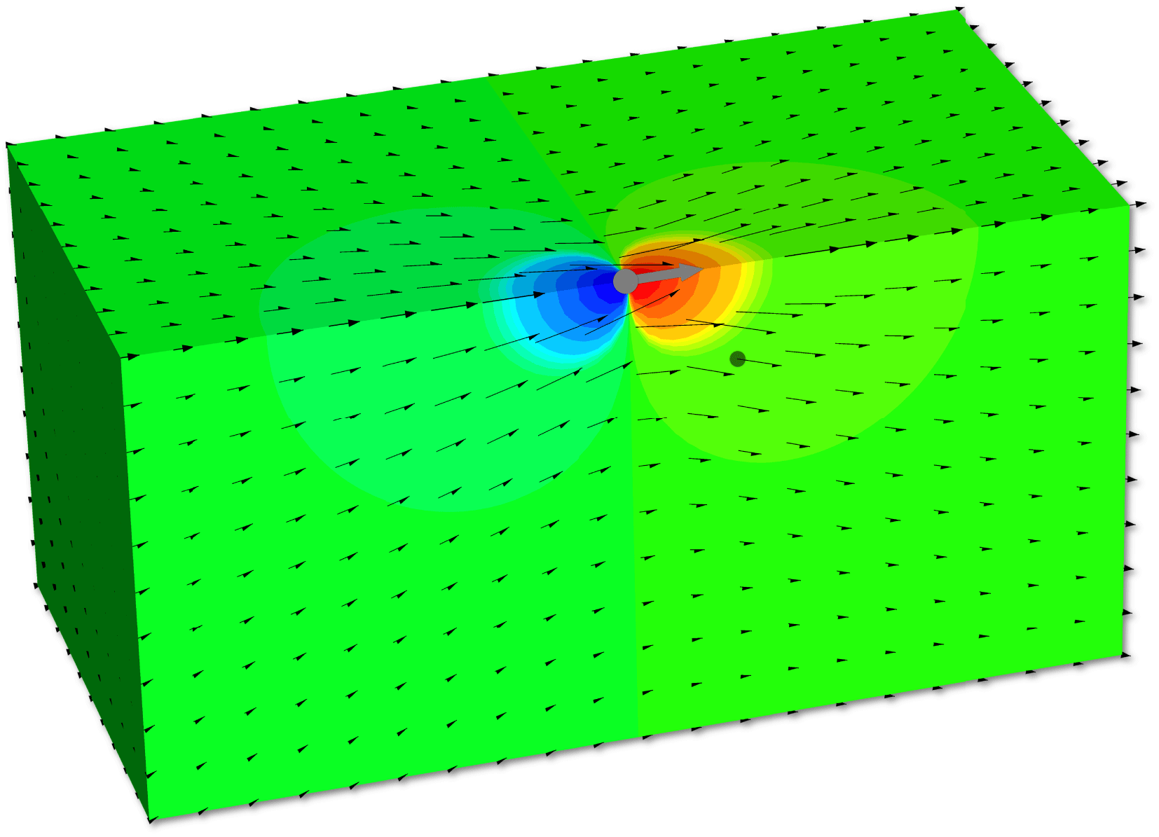
. From dimensional considerations based on the Stokes equations and considering three-dimensional space, we can conclude that, far from the point source, the velocity, pressure and stress fields decay with distance as (see also figure 4)
 $$\begin{eqnarray}\left|\boldsymbol{u}\right|=O(r^{-1}),\quad p=O(r^{-2}),\quad \left|\boldsymbol{n}\boldsymbol{\cdot }\unicode[STIX]{x1D748}\right|=O(r^{-2}).\end{eqnarray}$$
These rates of decay will be important in some of the forthcoming derivations. A reader can also verify that a point torque in three dimensions decays one power of
 $r$
faster.
Velocity field and pressure distribution (colour contours) produced by a point force in Stokes flow. The grey circle and arrow indicate the location and direction of the point source, respectively. The smaller dark grey circle represents a typical field point.

Of course, the mathematical problem posed in (4.1) can be solved, e.g. a convenient procedure is to use the Fourier transform. In three dimensions, the solution can be written compactly as (see also figure 4)
 $$\begin{eqnarray}\displaystyle & \displaystyle \boldsymbol{u}(\boldsymbol{r})=\unicode[STIX]{x1D642}(\boldsymbol{r},\boldsymbol{r}_{s})\boldsymbol{\cdot }\boldsymbol{F},\quad \text{where }\unicode[STIX]{x1D642}(\boldsymbol{r},\boldsymbol{r}_{s})=\frac{1}{8\unicode[STIX]{x03C0}\unicode[STIX]{x1D707}}\left(\frac{\unicode[STIX]{x1D644}}{\text{}\underline{r}}+\frac{\text{}\underline{\boldsymbol{r}}\text{}\underline{\boldsymbol{r}}}{\text{}\underline{r}^{3}}\right), & \displaystyle\end{eqnarray}$$
 $$\begin{eqnarray}\displaystyle & \displaystyle p(\boldsymbol{r})=\frac{\text{}\underline{\boldsymbol{r}}}{4\unicode[STIX]{x03C0}\text{}\underline{r}^{3}}\boldsymbol{\cdot }\boldsymbol{F}, & \displaystyle\end{eqnarray}$$
 $$\begin{eqnarray}\displaystyle & \displaystyle \unicode[STIX]{x1D748}(\boldsymbol{r})=\unicode[STIX]{x1D643}(\boldsymbol{r},\boldsymbol{r}_{s})\boldsymbol{\cdot }\boldsymbol{F},\quad \text{where }\unicode[STIX]{x1D643}(\boldsymbol{r},\boldsymbol{r}_{s})=-\frac{3}{4\unicode[STIX]{x03C0}}\frac{\text{}\underline{\boldsymbol{r}}\text{}\underline{\boldsymbol{r}}\text{}\underline{\boldsymbol{r}}}{\text{}\underline{r}^{5}}, & \displaystyle\end{eqnarray}$$
 $\text{}\underline{\boldsymbol{r}}=\boldsymbol{r}-\boldsymbol{r}_{s}$
with
 $\text{}\underline{r}=|\text{}\underline{\boldsymbol{r}}|$
. The second-rank tensor
 $\unicode[STIX]{x1D642}$
is the Green’s function for the velocity field in Stokes flow and the corresponding stress is characterized by the third-rank tensor
 $\unicode[STIX]{x1D643}$
.
4.2 Symmetry of the Green’s function
Imagine a general configuration, such as a domain containing many fixed obstacles. For flow resulting from a point force
 $\boldsymbol{F}_{A}$
at location
 $\boldsymbol{r}_{A}$
in this configuration, the Stokes momentum equation can be written as
 $$\begin{eqnarray}\unicode[STIX]{x1D735}\boldsymbol{\cdot }\unicode[STIX]{x1D748}_{A}+\boldsymbol{F}_{A}\unicode[STIX]{x1D6FF}(\boldsymbol{r}-\boldsymbol{r}_{A})=\mathbf{0}.\end{eqnarray}$$
The Green’s function
 $\unicode[STIX]{x1D642}$
of (4.4) then gives the velocity distribution through
 $\boldsymbol{u}_{A}=\unicode[STIX]{x1D642}(\boldsymbol{r},\boldsymbol{r}_{A})\boldsymbol{\cdot }\boldsymbol{F}_{A}$
.
Now, consider a second Stokes flow with a point force
 $\boldsymbol{F}_{B}$
at position
 $\boldsymbol{r}_{B}$
, i.e.
 $\unicode[STIX]{x1D735}\boldsymbol{\cdot }\unicode[STIX]{x1D748}_{B}+\boldsymbol{F}_{B}\,\unicode[STIX]{x1D6FF}(\boldsymbol{r}-\boldsymbol{r}_{B})=\mathbf{0}$
. The corresponding velocity field is denoted
 $\boldsymbol{u}_{B}$
. Next, apply the reciprocal theorem (3.12) to these two distinct motions driven by
 $\boldsymbol{F}_{A}$
and
 $\boldsymbol{F}_{B}$
, within a domain
 $V$
bounded by surfaces
 $S$
, to obtain
 $$\begin{eqnarray}\displaystyle & & \displaystyle \int _{S}\boldsymbol{n}\boldsymbol{\cdot }\unicode[STIX]{x1D748}_{A}\boldsymbol{\cdot }\boldsymbol{u}_{B}\,\text{d}S-\int _{S}\boldsymbol{n}\boldsymbol{\cdot }\unicode[STIX]{x1D748}_{B}\boldsymbol{\cdot }\boldsymbol{u}_{A}\,\text{d}S\nonumber\\ \displaystyle & & \displaystyle \quad =\int _{V}\boldsymbol{u}_{B}\boldsymbol{\cdot }\boldsymbol{F}_{A}\,\unicode[STIX]{x1D6FF}(\boldsymbol{r}-\boldsymbol{r}_{A})\,\text{d}V-\int _{V}\boldsymbol{u}_{A}\boldsymbol{\cdot }\boldsymbol{F}_{B}\,\unicode[STIX]{x1D6FF}(\boldsymbol{r}-\boldsymbol{r}_{B})\,\text{d}V.\end{eqnarray}$$
Assuming no-slip condition on all boundaries, we observe that (4.5) simplifies to
 $\boldsymbol{u}_{B}(\boldsymbol{r}_{A})\boldsymbol{\cdot }\boldsymbol{F}_{A}=\boldsymbol{u}_{A}(\boldsymbol{r}_{B})\boldsymbol{\cdot }\boldsymbol{F}_{B}$
. Thus, using the definition of the Green’s function, we arrive at
 $$\begin{eqnarray}\boldsymbol{F}_{A}\boldsymbol{\cdot }\unicode[STIX]{x1D642}(\boldsymbol{r}_{A},\boldsymbol{r}_{B})\boldsymbol{\cdot }\boldsymbol{F}_{B}=\boldsymbol{F}_{B}\boldsymbol{\cdot }\unicode[STIX]{x1D642}(\boldsymbol{r}_{B},\boldsymbol{r}_{A})\boldsymbol{\cdot }\boldsymbol{F}_{A}.\end{eqnarray}$$
Therefore, we conclude

which corresponds to the idea of exchanging ‘source’ and ‘receiver’.
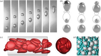
(a) Sequence of photographs depicting the translation of two interacting air bubbles in a large container of corn syrup and (b) the corresponding simulation using the boundary integral formulation described in § 4.4 (adapted from Manga & Stone Reference Manga and Stone1993). (c,d) Two additional examples of numerical simulations developed from the integral representation of the solution to the Stokes equations. (c) Flow of red blood cells in a cylindrical tube (adapted, with permission, from Zhao et al. Reference Zhao, Isfahani, Olson and Freund2010). (d) Flow of droplets through a porous media; the droplets have the same viscosity as the suspending fluid (adapted, with permission, from Zinchenko & Davis Reference Zinchenko and Davis2008).

4.3 An integral equation for translation of a rigid particle
Integral equations find a variety of uses in fluid mechanics, specially in potential and Stokes flows. For example, drop deformation and the flow of suspensions (of rigid or soft particles such as red blood cells) are common application areas (see figure 5). Here, we first develop an equation for the velocity distribution due to the motion of a rigid particle in an infinite domain (e.g. Youngren & Acrivos Reference Youngren and Acrivos1975); our presentation closely follows Stone & Duprat (Reference Stone, Duprat, Duprat and Stone2016).
We begin with the reciprocal theorem using as the auxiliary field the velocity and stress from the point-force problem (4.3), which is
 $\unicode[STIX]{x1D735}\boldsymbol{\cdot }\hat{\unicode[STIX]{x1D748}}+\hat{\boldsymbol{F}}\,\unicode[STIX]{x1D6FF}(\boldsymbol{r}-\boldsymbol{r}_{s})=\mathbf{0}$
and
 $\unicode[STIX]{x1D735}\boldsymbol{\cdot }\hat{\boldsymbol{u}}=0$
. The integral identify (3.12) becomes
 $$\begin{eqnarray}\int _{S}\boldsymbol{n}\boldsymbol{\cdot }\unicode[STIX]{x1D748}\boldsymbol{\cdot }\hat{\boldsymbol{u}}\,\text{d}S=\int _{S}\boldsymbol{n}\boldsymbol{\cdot }\hat{\unicode[STIX]{x1D748}}\boldsymbol{\cdot }\boldsymbol{u}\,\text{d}S-\hat{\boldsymbol{F}}\boldsymbol{\cdot }\int _{V}\unicode[STIX]{x1D6FF}(\boldsymbol{r}-\boldsymbol{r}_{s})\boldsymbol{u}\,\text{d}V,\end{eqnarray}$$
where
 $\boldsymbol{r}$
is the integration variable. The boundary
 $S$
indicates both the surface of the particle
 $S_{p}$
and a bounding surface at infinity
 $S_{\infty }$
. We note that we can neglect contributions in (4.8) from a surface at ‘infinity’ since in the far field, as
 $r\rightarrow \infty$
, the kernels of the two surface integrals decay at least as fast as
 $O(r^{-3})$
while
 $\text{d}S$
grows as
 $O(r^{2})$
. Next, using the form of the point-force solution (4.3) and the properties of the delta function, we find
 $$\begin{eqnarray}\left.\begin{array}{@{}ll@{}}1, & \text{if }\boldsymbol{r}_{s}\in V\\ 1/2, & \text{if }\boldsymbol{r}_{s}\in S_{p}\\ 0, & \text{if }\boldsymbol{r}_{s}\not \in V\end{array}\right\}\hat{\boldsymbol{F}}\boldsymbol{\cdot }\boldsymbol{u}\left(\boldsymbol{r}_{s}\right)=-\hat{\boldsymbol{F}}\boldsymbol{\cdot }\int _{S_{p}}\boldsymbol{n}\boldsymbol{\cdot }\unicode[STIX]{x1D748}\boldsymbol{\cdot }\unicode[STIX]{x1D642}(\boldsymbol{r},\boldsymbol{r}_{s})\,\text{d}S_{\boldsymbol{r}}+\hat{\boldsymbol{F}}\boldsymbol{\cdot }\int _{S_{p}}\boldsymbol{n}\boldsymbol{\cdot }\unicode[STIX]{x1D643}(\boldsymbol{r},\boldsymbol{r}_{s})\boldsymbol{\cdot }\boldsymbol{u}\,\text{d}S_{\boldsymbol{r}},\end{eqnarray}$$
where we have allowed for different choices of the location of the point force
 $\boldsymbol{r}_{s}$
, i.e. inside the domain, outside the domain and on the surface; also, we have assumed the surface is smooth, which yields the factor
 $1/2$
for positions on the surface,
 $\boldsymbol{r}_{s}\in S_{p}$
. The notation in (4.9) has been chosen to clarify that
 $\boldsymbol{r}$
is the integration variable. Since
 $\unicode[STIX]{x1D60E}_{ij}(\boldsymbol{r},\boldsymbol{r}_{s})=\unicode[STIX]{x1D60E}_{ji}(\boldsymbol{r}_{s},\boldsymbol{r})$
, see (4.7), and the vector
 $\hat{\boldsymbol{F}}$
is otherwise arbitrary in (4.9), we find the result
 $$\begin{eqnarray}\left.\begin{array}{@{}ll@{}}1, & \text{if }\boldsymbol{r}_{s}\in V\\ 1/2, & \text{if }\boldsymbol{r}_{s}\in S_{p}\\ 0, & \text{if }\boldsymbol{r}_{s}\not \in V\end{array}\right\}\boldsymbol{u}\left(\boldsymbol{r}_{s}\right)=-\int _{S_{p}}\unicode[STIX]{x1D642}(\boldsymbol{r}_{s},\boldsymbol{r})\boldsymbol{\cdot }\boldsymbol{f}\,\text{d}S_{\boldsymbol{r}}+\int _{S_{p}}\boldsymbol{n}\boldsymbol{\cdot }\unicode[STIX]{x1D643}(\boldsymbol{r},\boldsymbol{r}_{s})\boldsymbol{\cdot }\boldsymbol{u}\,\text{d}S_{\boldsymbol{r}},\end{eqnarray}$$
which is an integral equation relating the velocity and surface traction (
 $\boldsymbol{f}=\boldsymbol{n}\boldsymbol{\cdot }\unicode[STIX]{x1D748}$
) distributions on
 $S_{p}$
, the surface of the object.
There are many examples where the integral equation (4.10) is the starting point for numerical solutions. For example, if a rigid particle translates, then the velocity on the surface is known and (4.10) is an integral equation of the first kind for the unknown distribution of surface traction
 $\boldsymbol{f}$
. Similar ideas apply to particles near boundaries, where the Green’s functions
 $\unicode[STIX]{x1D642}$
and
 $\unicode[STIX]{x1D643}$
may be chosen to automatically satisfy the no-slip boundary condition on stationary surfaces. An excellent reference for the many applications of these integral equation methods to low-Reynolds-number motions is Pozrikidis (Reference Pozrikidis1992).
We next specialize (4.10) to the case of a rigid (smooth) rigid body translating with velocity
 $\boldsymbol{U}$
. Note that the stress version of the point-force equation is
 $$\begin{eqnarray}\unicode[STIX]{x1D735}\boldsymbol{\cdot }\unicode[STIX]{x1D643}+\unicode[STIX]{x1D6FF}\left(\boldsymbol{r}-\boldsymbol{r}_{s}\right)\unicode[STIX]{x1D644}=\mathbf{0}.\end{eqnarray}$$
Focusing on the second integral on the right-hand side of (4.10) and using the divergence theorem, then for points on the surface
 $S_{p}$
surrounding the particle volume
 $V_{p}$
, where the velocity
 $\boldsymbol{u}=\boldsymbol{U}$
, we have (
 $\boldsymbol{r}\in S_{p}$
)
 $$\begin{eqnarray}\displaystyle \int _{S_{p}}\boldsymbol{n}\boldsymbol{\cdot }\unicode[STIX]{x1D643}\boldsymbol{\cdot }\boldsymbol{u}\,\text{d}S_{\boldsymbol{r}} & = & \displaystyle \int _{V_{p}}\unicode[STIX]{x1D735}\boldsymbol{\cdot }\unicode[STIX]{x1D643}\,\text{d}V_{\boldsymbol{r}}\boldsymbol{\cdot }\boldsymbol{U}\nonumber\\ \displaystyle & = & \displaystyle -\int _{V_{p}}\unicode[STIX]{x1D6FF}(\boldsymbol{r}-\boldsymbol{r}_{s})\,\text{d}V_{\boldsymbol{r}}\left(\unicode[STIX]{x1D644}\boldsymbol{\cdot }\boldsymbol{U}\right)\nonumber\\ \displaystyle & = & \displaystyle \left\{\begin{array}{@{}ll@{}}0 & \text{if }\boldsymbol{r}_{s}\in V\\ -\boldsymbol{U}/2 & \text{if }\boldsymbol{r}_{s}\in S_{p}.\end{array}\right.\end{eqnarray}$$
After interchanging
 $\boldsymbol{r}$
and
 $\boldsymbol{r}_{s}$
, equation (4.10) reduces to
 $$\begin{eqnarray}\boldsymbol{u}(\boldsymbol{r})=-\int _{S_{p}}\unicode[STIX]{x1D642}(\boldsymbol{r},\boldsymbol{r}_{s})\boldsymbol{\cdot }\boldsymbol{f}(\boldsymbol{r}_{s})\,\text{d}S_{\boldsymbol{r}_{s}}\quad (\text{valid for }\boldsymbol{r}\in S_{p},V),\end{eqnarray}$$
which is an integral equation of the first kind for the unknown surface traction distribution
 $\boldsymbol{f}$
that accompanies translation
 $\boldsymbol{U}$
of the rigid particle. The total force on the particle follows from
 $\int _{S_{p}}\boldsymbol{f}\,\text{d}S$
. The corresponding velocity field about the particle can then be evaluated using (4.13).
4.4 An integral equation for a two-phase flow
Let us now consider the case of a neutrally buoyant droplet of Newtonian fluid (viscosity
 $\hat{\unicode[STIX]{x1D707}}$
) immersed in a second immiscible Newtonian fluid (viscosity
 $\unicode[STIX]{x1D707}$
), which has the undisturbed velocity distribution
 $\boldsymbol{U}_{\infty }(\boldsymbol{r})$
at large distances from the drop. We can expect that the drop translates and deforms, depending on the viscosity ratio
 $\hat{\unicode[STIX]{x1D707}}/\unicode[STIX]{x1D707}$
and the details of
 $\boldsymbol{U}_{\infty }(\boldsymbol{r})$
, e.g. the strain rate and vorticity of the undisturbed flow. In the equations below, we always use
 $\boldsymbol{n}$
to denote the unit normal vector directed into the external fluid away from the drop interface
 $S_{i}$
. Several examples of these kinds of problems are shown in figure 5, where the solutions are produced using integral equation methods.
We begin with the external flow (domain
 $V$
) written as (4.10), although now accounting for the undisturbed flow,
 $$\begin{eqnarray}\left.\begin{array}{@{}ll@{}}1, & \text{if }\boldsymbol{r}_{s}\in V\\ 1/2, & \text{if }\boldsymbol{r}_{s}\in S_{i}\\ 0, & \text{if }\boldsymbol{r}_{s}\not \in V\end{array}\right\}\boldsymbol{u}(\boldsymbol{r}_{s})=\boldsymbol{U}_{\infty }(\boldsymbol{r}_{s})-\int _{S_{i}}\boldsymbol{n}\boldsymbol{\cdot }\unicode[STIX]{x1D748}\boldsymbol{\cdot }\unicode[STIX]{x1D642}(\boldsymbol{r},\boldsymbol{r}_{s})\,\text{d}S_{\boldsymbol{r}}+\int _{S_{i}}\boldsymbol{n}\boldsymbol{\cdot }\unicode[STIX]{x1D643}(\boldsymbol{r},\boldsymbol{r}_{s})\boldsymbol{\cdot }\boldsymbol{u}\,\text{d}S_{\boldsymbol{r}}.\end{eqnarray}$$
For the corresponding internal flow, and accounting for the direction of
 $\boldsymbol{n}$
, we can write
 $$\begin{eqnarray}\left.\begin{array}{@{}ll@{}}0, & \text{if }\boldsymbol{r}_{s}\in V\\ 1/2, & \text{if }\boldsymbol{r}_{s}\in S_{i}\\ 1, & \text{if }\boldsymbol{r}_{s}\not \in V\end{array}\right\}\hat{\boldsymbol{u}}(\boldsymbol{r}_{s})=\frac{\unicode[STIX]{x1D707}}{\hat{\unicode[STIX]{x1D707}}}\int _{S_{i}}\boldsymbol{n}\boldsymbol{\cdot }\hat{\unicode[STIX]{x1D748}}\boldsymbol{\cdot }\unicode[STIX]{x1D642}(\boldsymbol{r},\boldsymbol{r}_{s})\,\text{d}S_{\boldsymbol{r}}-\int _{S_{i}}\boldsymbol{n}\boldsymbol{\cdot }\unicode[STIX]{x1D643}(\boldsymbol{r},\boldsymbol{r}_{s})\boldsymbol{\cdot }\hat{\boldsymbol{u}}\,\text{d}S_{\boldsymbol{r}},\end{eqnarray}$$
where the appearance of
 $\unicode[STIX]{x1D707}/\hat{\unicode[STIX]{x1D707}}$
on the right-hand side occurs owing to the definition of
 $\unicode[STIX]{x1D642}$
that includes the viscosity
 $\unicode[STIX]{x1D707}$
of the continuous phase fluid. At the boundary between the two immiscible fluids, the boundary condition for the stress jump, assuming a constant surface tension
 $\unicode[STIX]{x1D6FE}$
, is written as
 $$\begin{eqnarray}\boldsymbol{n}\boldsymbol{\cdot }\unicode[STIX]{x1D748}-\boldsymbol{n}\boldsymbol{\cdot }\hat{\unicode[STIX]{x1D748}}=\unicode[STIX]{x1D6FE}\unicode[STIX]{x1D705}\boldsymbol{n},\end{eqnarray}$$
where
 $\unicode[STIX]{x1D705}$
is twice the mean curvature of the interface.
Next, we assume that the point force is located at
 $\boldsymbol{r}_{s}\in S_{i}$
, where
 $\boldsymbol{u}=\hat{\boldsymbol{u}}$
. Adding (4.14) to
 $\hat{\unicode[STIX]{x1D707}}/\unicode[STIX]{x1D707}$
times (4.15) and applying the stress jump condition leads to an equation for the velocity distribution along the interface
 $$\begin{eqnarray}\frac{1}{2}\left(1+\frac{\hat{\unicode[STIX]{x1D707}}}{\unicode[STIX]{x1D707}}\right)\boldsymbol{u}(\boldsymbol{r}_{s})=\boldsymbol{U}_{\infty }(\boldsymbol{r}_{s})-\unicode[STIX]{x1D6FE}\int _{S_{i}}\unicode[STIX]{x1D705}\,\boldsymbol{n}\,\boldsymbol{\cdot }\unicode[STIX]{x1D642}(\boldsymbol{r},\boldsymbol{r}_{s})\,\text{d}S_{\boldsymbol{r}}+\left(1-\frac{\hat{\unicode[STIX]{x1D707}}}{\unicode[STIX]{x1D707}}\right)\int _{S_{i}}\boldsymbol{n}\boldsymbol{\cdot }\unicode[STIX]{x1D643}(\boldsymbol{r},\boldsymbol{r}_{s})\boldsymbol{\cdot }\,\boldsymbol{u}\,\text{d}S_{\boldsymbol{r}}.\end{eqnarray}$$
This result was first established by Rallison & Acrivos (Reference Rallison and Acrivos1978).
For the special case of equal viscosity fluids,
 $\hat{\unicode[STIX]{x1D707}}/\unicode[STIX]{x1D707}=1$
, then, upon recognizing the symmetry of
 $\unicode[STIX]{x1D642}$
and interchanging
 $\boldsymbol{r}$
and
 $\boldsymbol{r}_{s}$
, we have
 $$\begin{eqnarray}\boldsymbol{u}(\boldsymbol{r})=\boldsymbol{U}_{\infty }(\boldsymbol{r})-\unicode[STIX]{x1D6FE}\int _{S_{i}}\unicode[STIX]{x1D705}\,\unicode[STIX]{x1D642}(\boldsymbol{r},\boldsymbol{r}_{s})\boldsymbol{\cdot }\,\boldsymbol{n}\,\text{d}S_{\boldsymbol{r}_{s}}.\end{eqnarray}$$
The velocity field is determined for a given shape, i.e. the shape dictates the distribution of curvature (or
 $\unicode[STIX]{x1D705}$
) and an integration over the surface gives the velocity of the interface, which then determines the change of the shape, etc.
5 Particle mobility
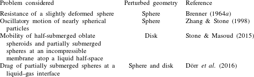
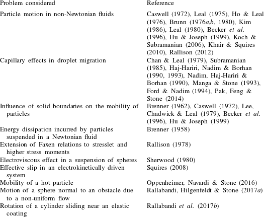
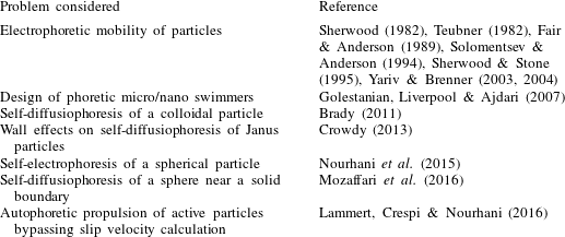
In suspension mechanics, it is important to calculate the force and torque on individual objects, or determine their equivalent resistance or mobility tensors. Such information is critical for understanding the behaviour of the particles and for how they interact hydrodynamically with one another. The suspended particles can be rigid objects, droplets, cells, vesicles, etc. Their mobility is affected by many factors including their shape, deformability, orientation, surface condition, permeability (if they are porous), flow Reynolds number, proximity to confining boundaries, rheological properties of the surrounding fluid, etc. In this section, we focus on small rigid particles and employ the reciprocal identity (3.12) to first prove a reverse-flow theorem and some symmetries of the resistance tensors. We then derive asymptotic expressions describing the influence of some of the factors mentioned above on the hydrodynamic force experienced by a particle. A list of representative studies that use the reciprocal theorem to investigate these kinds of problems is given at the end of this section (see table 2).
5.1 Invariance of the drag on an object to reversal of motion
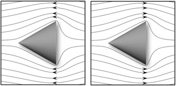
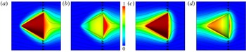
Consider an arbitrarily shaped particle in translation when the Reynolds number is small and the Stokes equations apply. For example, the object could be conical with a pointy end and a blunt back side. It is natural to think that the drag on the object will be different if the object translates point first versus translating with its blunt end leading (see figure 6). In fact, in the Stokes-flow limit, we will now see that the magnitude of the drag force does not change when the direction of translation is reversed.
Invariance of streamlines to flow reversal in an axisymmetric Stokes flow past a cone. The flow field is calculated numerically using a second-order finite-volume method. The figure is adapted from Vandadi, Jafari Kang & Masoud (Reference Vandadi, Jafari Kang and Masoud2016).

To study this problem, suppose we have an arbitrarily shaped particle (surface
 $S_{p}$
) translating with velocity
 $\boldsymbol{U}$
. We also consider the same particle translating in the opposite direction, velocity
 $-\boldsymbol{U}$
, and denote this second problem with the overhat symbol
 $(\hat{~})$
. Neglecting the body forces (
 $\boldsymbol{b}$
and
 $\hat{\boldsymbol{b}}$
), we start with the reciprocal theorem (3.12)
 $$\begin{eqnarray}\int _{S}\boldsymbol{n}\boldsymbol{\cdot }\unicode[STIX]{x1D748}\boldsymbol{\cdot }\hat{\boldsymbol{u}}\,\text{d}S=\int _{S}\boldsymbol{n}\boldsymbol{\cdot }\hat{\unicode[STIX]{x1D748}}\boldsymbol{\cdot }\boldsymbol{u}\,\text{d}S.\end{eqnarray}$$
Since the boundary velocities are specified and the kernels decay sufficiently fast for contributions from surfaces at infinity to vanish, we simplify the equation to
 $$\begin{eqnarray}-\boldsymbol{U}\boldsymbol{\cdot }\int _{S_{p}}\boldsymbol{n}\boldsymbol{\cdot }\unicode[STIX]{x1D748}\,\text{d}S=\boldsymbol{U}\boldsymbol{\cdot }\int _{S_{p}}\boldsymbol{n}\boldsymbol{\cdot }\hat{\unicode[STIX]{x1D748}}\,\text{d}S.\end{eqnarray}$$
The integrals are simply the hydrodynamic force on the particle for the given motion. Thus, we conclude that the drag force (the force opposite to the direction of motion) is the same when the direction of translation is reversed. This conclusion is true for an arbitrarily shaped object. So, a cone-shaped object in a low-Reynolds-number flow has the same drag independent of whether it leads with its pointy or blunt end, which of course is in sharp contrast with the corresponding familiar high-Reynolds-number motions. That the drag remains unchanged under the motion reversal is the direct consequence of the invariance of the flow streamlines to the change in the direction of particle motion – see e.g. figure 6 and also the experiment of Taylor (Reference Taylor1960), where he elegantly demonstrates the reversibility of flow for a Taylor–Couette configuration.
5.2 Symmetries of resistance tensors
To describe the influence of particles on the bulk flow (mean velocity
 $\boldsymbol{U}_{\infty }$
and vorticity
 $\unicode[STIX]{x1D74E}_{\infty }$
) of a suspension, it is necessary to determine the particle translational velocity
 $\boldsymbol{U}$
, relative to
 $\boldsymbol{U}_{\infty }$
, and rotational velocity
 $\unicode[STIX]{x1D734}$
, relative to
 $\unicode[STIX]{x1D74E}_{\infty }$
, as a function of the externally applied forces
 $\boldsymbol{F}_{e}$
and torques
 $\boldsymbol{L}_{e}$
. In addition, the macroscopic rheology is affected since rigid particles, or soft constituents with a surface tension and/or elasticity, do not deform identically with the local fluid velocity. Then, it is also necessary to consider the rate of strain tensor of the external flow
 $\unicode[STIX]{x1D640}_{\infty }$
and the particle response to strain, which is referred to as the stresslet
 $\unicode[STIX]{x1D64E}$
(see e.g. Batchelor Reference Batchelor1970; Guazzelli & Morris Reference Guazzelli and Morris2011), defined for rigid particles as
 $$\begin{eqnarray}\unicode[STIX]{x1D64E}=\frac{1}{2}\int _{S_{p}}\left(\boldsymbol{r}\boldsymbol{n}\boldsymbol{\cdot }\unicode[STIX]{x1D748}+\boldsymbol{n}\boldsymbol{\cdot }\unicode[STIX]{x1D748}\boldsymbol{r}\right)\text{d}S,\end{eqnarray}$$
where
 $\boldsymbol{r}$
is a position vector measured from some origin.
Because of the linearity of the Stokes equations (see e.g. Happel & Brenner Reference Happel and Brenner1983), we expect a linear relation between the relative velocities
 $\boldsymbol{U}-\boldsymbol{U}_{\infty }$
,
 $\unicode[STIX]{x1D734}-\unicode[STIX]{x1D74E}_{\infty }/2$
, and
 $\unicode[STIX]{x1D640}_{\infty }$
and the generalized forces
 $\boldsymbol{F}_{e}$
,
 $\boldsymbol{L}_{e}$
, and
 $\unicode[STIX]{x1D64E}$
. Thus, we write
 $$\begin{eqnarray}\left(\begin{array}{@{}c@{}}\boldsymbol{F}_{e}\\ \boldsymbol{ L}_{e}\\ \unicode[STIX]{x1D64E}\end{array}\right)=\unicode[STIX]{x1D707}\left(\begin{array}{@{}ccc@{}}\unicode[STIX]{x1D64D}^{\mathit{FU}} & \unicode[STIX]{x1D64D}^{F\unicode[STIX]{x1D6FA}} & \unicode[STIX]{x1D64D}^{\mathit{FE}}\\ \unicode[STIX]{x1D64D}^{\mathit{LU}} & \unicode[STIX]{x1D64D}^{L\unicode[STIX]{x1D6FA}} & \unicode[STIX]{x1D64D}^{\mathit{LE}}\\ \unicode[STIX]{x1D64D}^{\mathit{SU}} & \unicode[STIX]{x1D64D}^{S\unicode[STIX]{x1D6FA}} & \unicode[STIX]{x1D64D}^{\mathit{SE}}\end{array}\right)\boldsymbol{\cdot }\left(\begin{array}{@{}c@{}}\boldsymbol{U}-\boldsymbol{U}_{\infty }\\ \unicode[STIX]{x1D734}-\unicode[STIX]{x1D74E}_{\infty }/2\\ \unicode[STIX]{x1D640}_{\infty }\end{array}\right),\end{eqnarray}$$
where superscripts are used to identify the relationships and the operations involving
 $\unicode[STIX]{x1D640}_{\infty }$
are in fact the double inner product
 $(:)$
. The
 $\unicode[STIX]{x1D64D}^{mn}$
are known as resistance tensors. The inverses are known as mobility tensors and give the generalized velocities from generalized forces. Some numerical approaches to simulating suspension flows utilize these relationships (Brady & Bossis Reference Brady and Bossis1988; Sierou & Brady Reference Sierou and Brady2001).
We note that
 $\unicode[STIX]{x1D64D}^{\mathit{FU}}$
,
 $\unicode[STIX]{x1D64D}^{F\unicode[STIX]{x1D6FA}}$
,
 $\unicode[STIX]{x1D64D}^{\mathit{LU}}$
and
 $\unicode[STIX]{x1D64D}^{L\unicode[STIX]{x1D6FA}}$
are second-rank tensors,
 $\unicode[STIX]{x1D64D}^{\mathit{FE}}$
,
 $\unicode[STIX]{x1D64D}^{\mathit{LE}}$
,
 $\unicode[STIX]{x1D64D}^{\mathit{SU}}$
and
 $\unicode[STIX]{x1D64D}^{S\unicode[STIX]{x1D6FA}}$
are third-rank tensors and
 $\unicode[STIX]{x1D64D}^{\mathit{SE}}$
is a fourth-rank tensor. Equation (5.4) appears to suggest that these nine tensors are needed to characterize the general resistance problem. As first discussed by Hinch (Reference Hinch1972), however, three pairs of the tensors are related. Also, the remaining three possess certain symmetries. We now show, for arbitrarily shaped particles, the properties of these tensors, which follow naturally from the reciprocal theorem. Using index notation, these properties are (Hinch Reference Hinch1972)


In order to demonstrate these identities, we make use of the reciprocal theorem for the two corresponding motions, e.g. to learn about
 $\unicode[STIX]{x1D64D}^{F\unicode[STIX]{x1D6FA}}$
we consider two distinct flows, a translation (to account for the force) and a rotation. Similarly, to learn about
 $\unicode[STIX]{x1D64D}^{\mathit{FU}}$
, we consider two distinct translational motions of the particles,
 $\boldsymbol{U}$
(set
 $\boldsymbol{U}_{\infty }=\mathbf{0}$
) and
 $\hat{\boldsymbol{U}}$
. For example, in (5.1), we wrote the reciprocal theorem, which for translational motions
 $\boldsymbol{U}$
and
 $\hat{\boldsymbol{U}}$
, and the force relations
 $\boldsymbol{F}_{e}=\unicode[STIX]{x1D707}\unicode[STIX]{x1D64D}^{\mathit{FU}}\boldsymbol{\cdot }\boldsymbol{U}$
and
 $\hat{\boldsymbol{F}}_{\!e}=\unicode[STIX]{x1D707}\unicode[STIX]{x1D64D}^{\mathit{FU}}\boldsymbol{\cdot }\hat{\boldsymbol{U}}$
, reduces to (contributions from bounding surfaces at large distances vanish for an unbounded configuration, and they also vanish for a rigid enclosure owing to the no-slip condition)
 $$\begin{eqnarray}\hat{\boldsymbol{U}}\boldsymbol{\cdot }\unicode[STIX]{x1D64D}^{\mathit{FU}}\boldsymbol{\cdot }\boldsymbol{U}=\boldsymbol{U}\boldsymbol{\cdot }\unicode[STIX]{x1D64D}^{\mathit{FU}}\boldsymbol{\cdot }\hat{\boldsymbol{U}}.\end{eqnarray}$$
Thus, we deduce the symmetry  . The important consequence is that for an arbitrarily shaped particle one might anticipate needing nine coefficients to express the force–velocity relationship expressed by
 $\unicode[STIX]{x1D64D}^{\mathit{FU}}$
, but in fact only six coefficients are required. Of course, for a sphere, isometry leads to
 $\unicode[STIX]{x1D64D}^{\mathit{FU}}=6\unicode[STIX]{x03C0}R\unicode[STIX]{x1D644}$
, with
 $R$
being the radius of the sphere.
In the same spirit, one can consider a translation
 $\boldsymbol{U}$
and rotation
 $\hat{\unicode[STIX]{x1D734}}$
, i.e.
 $\hat{\boldsymbol{u}}=\hat{\unicode[STIX]{x1D734}}\times \boldsymbol{r}$
of a particle. Then, the reciprocal theorem (5.1), with the definition of the resistance tensors leads to
 $$\begin{eqnarray}\int _{S}\boldsymbol{n}\boldsymbol{\cdot }\unicode[STIX]{x1D748}\boldsymbol{\cdot }(\hat{\unicode[STIX]{x1D734}}\times \boldsymbol{r})\,\text{d}S=\int _{S}\boldsymbol{n}\boldsymbol{\cdot }\hat{\unicode[STIX]{x1D748}}\boldsymbol{\cdot }\boldsymbol{U}\,\text{d}S\end{eqnarray}$$
or, as
 $\boldsymbol{F}_{e}=-\int _{S_{p}}\boldsymbol{n}\boldsymbol{\cdot }\unicode[STIX]{x1D748}\,\text{d}S$
and
 $\boldsymbol{L}_{e}=-\int _{S_{p}}\boldsymbol{r}\times \left(\boldsymbol{n}\boldsymbol{\cdot }\unicode[STIX]{x1D748}\right)\text{d}S$
, to
 $$\begin{eqnarray}\hat{\unicode[STIX]{x1D734}}\boldsymbol{\cdot }\unicode[STIX]{x1D64D}^{\mathit{LU}}\boldsymbol{\cdot }\boldsymbol{U}=\boldsymbol{U}\boldsymbol{\cdot }\unicode[STIX]{x1D64D}^{F\unicode[STIX]{x1D6FA}}\boldsymbol{\cdot }\hat{\unicode[STIX]{x1D734}}.\end{eqnarray}$$
Thus, we conclude  .
As an example of the tensors involving the rate of strain, it suffices to consider a rigid particle with surface velocity
 $\boldsymbol{u}=\unicode[STIX]{x1D640}\boldsymbol{\cdot }\boldsymbol{r}$
. Also, consider the same particle with the distinct rotational motion
 $\hat{\boldsymbol{u}}=\hat{\unicode[STIX]{x1D734}}\times \boldsymbol{r}$
. Substituting these surface velocity distributions into the reciprocal theorem yields
 $$\begin{eqnarray}\int _{S_{p}}\boldsymbol{n}\boldsymbol{\cdot }\unicode[STIX]{x1D748}\boldsymbol{\cdot }(\hat{\unicode[STIX]{x1D734}}\times \boldsymbol{r})\,\text{d}S=\unicode[STIX]{x1D640}\boldsymbol{ : }\int _{S_{p}}\boldsymbol{r}\boldsymbol{n}\boldsymbol{\cdot }\hat{\unicode[STIX]{x1D748}}\,\text{d}S\end{eqnarray}$$
and, as the tensors
 $\unicode[STIX]{x1D640}$
and
 $\unicode[STIX]{x1D64E}$
are symmetric, we find
 $$\begin{eqnarray}\boldsymbol{L}_{e}\boldsymbol{\cdot }\hat{\unicode[STIX]{x1D734}}=\unicode[STIX]{x1D640}\boldsymbol{ : }\hat{\unicode[STIX]{x1D64E}}.\end{eqnarray}$$
Using the definition of the resistance tensors, we can then write

Therefore, we conclude  .
As a final example, consider the fourth-rank tensor
 $\unicode[STIX]{x1D64D}^{\mathit{SE}}$
for which we consider two distinct straining motions, i.e. suppose surface velocity distributions
 $\boldsymbol{u}=\unicode[STIX]{x1D640}\boldsymbol{\cdot }\boldsymbol{r}$
and
 $\hat{\boldsymbol{u}}=\hat{\unicode[STIX]{x1D640}}\boldsymbol{\cdot }\boldsymbol{ r}$
. The reciprocal theorem then leads to
 $$\begin{eqnarray}\hat{\unicode[STIX]{x1D640}}\boldsymbol{ : }\unicode[STIX]{x1D64E}=\unicode[STIX]{x1D640}\boldsymbol{ : }\hat{\unicode[STIX]{x1D64E}}\quad \Rightarrow \quad \hat{\unicode[STIX]{x1D640}}\boldsymbol{ : }\unicode[STIX]{x1D64D}^{\mathit{SE}}\boldsymbol{ : }\unicode[STIX]{x1D640}=\unicode[STIX]{x1D640}\boldsymbol{ : }\unicode[STIX]{x1D64D}^{\mathit{SE}}\boldsymbol{ : }\hat{\unicode[STIX]{x1D640}}.\end{eqnarray}$$
It follows that  .
The reciprocal theorem has been used in a similar fashion to prove the symmetry properties of the resistance tensor in linear electrohydrodynamics (Felderhof Reference Felderhof1983), the effective viscosity tensor of a periodic suspension (Nunan & Keller Reference Nunan and Keller1984) and the surface mobility (slip) tensor for Stokes flows along arbitrarily patterned surfaces (Kamrin & Stone Reference Kamrin and Stone2011). Finally, we note that about the same time as Hinch’s analysis of the symmetries of the generalized force–velocity relation given by (5.4) (Hinch Reference Hinch1972), Hauge & Martin-Löf (Reference Hauge and Martin-Löf1973) discussed the reciprocal theorem for characterizing the general mobility problem in a study of the Langevin description of fluctuating hydrodynamics (Brownian motion) for small particles.
5.3 Lens-shaped particles: an example of non-trivial shapes studied with perturbation theory
For simple shapes that correspond to well-established coordinate systems – spheres, oblate and prolate spheroids and thin circular disks – analytical results valid for the zero-Reynolds-number limit for the force and torque are well known (e.g. Happel & Brenner Reference Happel and Brenner1983; Kim & Karrila Reference Kim and Karrila2005). For other shapes, or perhaps awkward or unusual shapes, numerical procedures are available. Nevertheless, for shapes that are ‘close by’ one of the shapes for which analytical results are known, then in some cases it is possible to utilize the reciprocal theorem in concert with a geometrical (domain) perturbation series to determine analytically the hydrodynamic force or torque; the idea of domain perturbation was introduced in § 2.2.1. Below, we describe two examples of these ideas and list several others in table 1.
Examples of studies that employed a geometrical perturbation in conjunction with the reciprocal theorem for calculating the particle mobility.

Consider the edgewise translation of a lens of radius
 $R$
(see figure 7) with the velocity
 $\boldsymbol{U}=U\boldsymbol{e}$
with
 $U=|\boldsymbol{U}|$
and
 $\boldsymbol{e}$
being the unit vector in the direction of motion. We seek to determine the hydrodynamic force on the particle
 $\boldsymbol{F}=F\boldsymbol{e}$
as a function of its aspect ratio
 $\unicode[STIX]{x1D700}$
, which we shall assume is small, i.e.
 $\unicode[STIX]{x1D700}\ll 1$
. In this limit, the surface of the lens can be described in terms of a perturbation expansion from a circular disk, whose surface is denoted
 $S_{d}$
. Let
 $(\unicode[STIX]{x1D71A},\unicode[STIX]{x1D711},z)$
be cylindrical coordinates, where
 $z=0$
represents the plane of symmetry normal to the axis of revolution and
 $\unicode[STIX]{x1D71A}=0$
passes through the centre of the lens. In these coordinates, the surface of the particle can be described as
 $$\begin{eqnarray}z=\pm \,\frac{R}{\sin \unicode[STIX]{x1D6E9}}\left[\sqrt{1-\left(\frac{\unicode[STIX]{x1D71A}}{R}\right)^{2}\sin ^{2}\unicode[STIX]{x1D6E9}}+\cos \unicode[STIX]{x1D6E9}\right]=R\left[\unicode[STIX]{x1D700}h(\unicode[STIX]{x1D71A})+O(\unicode[STIX]{x1D700}^{2})\right],\end{eqnarray}$$
where
 $R$
is the radius of the particle,
 $\unicode[STIX]{x1D700}=z_{max}/R=\cot (\unicode[STIX]{x1D6E9}/2)$
, and
 $h(\unicode[STIX]{x1D71A})=\pm [1-(\unicode[STIX]{x1D71A}/R)^{2}]$
. The geometric definition of the opening angle
 $\unicode[STIX]{x1D6E9}$
for a lens is shown in figure 7(c).
A thin oblate spheroid (a) or a slender lens (c) can be approximated geometrically as a perturbed disk (b).

It is then natural to write the fluid velocity
 $\boldsymbol{u}$
, fluid stress
 $\unicode[STIX]{x1D748}$
and hydrodynamic force
 $\boldsymbol{F}$
corresponding to the actual shape in the forms
 $$\begin{eqnarray}\displaystyle & \displaystyle \boldsymbol{u}=\boldsymbol{u}^{(0)}+\unicode[STIX]{x1D700}\boldsymbol{u}^{(1)}+O(\unicode[STIX]{x1D700}^{2}), & \displaystyle\end{eqnarray}$$
 $$\begin{eqnarray}\displaystyle & \displaystyle \unicode[STIX]{x1D748}=\unicode[STIX]{x1D748}^{(0)}+\unicode[STIX]{x1D700}\unicode[STIX]{x1D748}^{(1)}+O(\unicode[STIX]{x1D700}^{2}), & \displaystyle\end{eqnarray}$$
 $$\begin{eqnarray}\displaystyle & \displaystyle \boldsymbol{F}=\boldsymbol{F}^{(0)}+\unicode[STIX]{x1D700}\boldsymbol{F}^{(1)}+O(\unicode[STIX]{x1D700}^{2}), & \displaystyle\end{eqnarray}$$
 resulting in (see also § 2.2.1)

To proceed, we represent the no-slip velocity at the actual surface of the particle in terms of a Taylor series about
 $z=0$
as (see also § 2.2.1)
 $$\begin{eqnarray}\boldsymbol{U}=\boldsymbol{u}^{\left(0\right)}+\unicode[STIX]{x1D700}\left[\boldsymbol{u}^{\left(1\right)}+R\,h(\unicode[STIX]{x1D71A})\frac{\unicode[STIX]{x2202}\boldsymbol{u}^{\left(0\right)}}{\unicode[STIX]{x2202}z}\right]+O(\unicode[STIX]{x1D700}^{2}),\end{eqnarray}$$
where
 $\boldsymbol{u}^{(0)}$
,
 $\boldsymbol{u}^{(1)}$
and
 $\unicode[STIX]{x2202}\boldsymbol{u}^{(0)}/\unicode[STIX]{x2202}z$
are all evaluated at
 $z=0$
. At
 $O(1)$
, we must solve for the edgewise translation of a circular disk with the boundary condition
 $$\begin{eqnarray}\boldsymbol{u}^{\left(0\right)}=\boldsymbol{U},\quad \text{at }z=0\quad (r\leqslant R).\end{eqnarray}$$
The solution to this problem is known analytically (e.g. Ranger Reference Ranger1978; Davis Reference Davis1990; Tanzosh & Stone Reference Tanzosh and Stone1996) as
 $$\begin{eqnarray}\displaystyle & \displaystyle u_{r}^{(0)}(\unicode[STIX]{x1D71A},\unicode[STIX]{x1D711},z)=\frac{2\,U\cos \unicode[STIX]{x1D711}}{3\unicode[STIX]{x03C0}}\left[3\cot ^{-1}\unicode[STIX]{x1D702}-\frac{\unicode[STIX]{x1D702}\,\unicode[STIX]{x1D701}^{2}}{\unicode[STIX]{x1D702}^{2}+\unicode[STIX]{x1D701}^{2}}+\frac{\unicode[STIX]{x1D702}^{3}(1-\unicode[STIX]{x1D701}^{2})}{(1+\unicode[STIX]{x1D702}^{2})(\unicode[STIX]{x1D702}^{2}+\unicode[STIX]{x1D701}^{2})}\right], & \displaystyle\end{eqnarray}$$
 $$\begin{eqnarray}\displaystyle & \displaystyle u_{\unicode[STIX]{x1D711}}^{(0)}(\unicode[STIX]{x1D71A},\unicode[STIX]{x1D711},z)=\frac{2\,U\sin \unicode[STIX]{x1D711}}{3\unicode[STIX]{x03C0}}\left[-3\cot ^{-1}\unicode[STIX]{x1D702}+\frac{\unicode[STIX]{x1D702}\,\unicode[STIX]{x1D701}^{2}}{\unicode[STIX]{x1D702}^{2}+\unicode[STIX]{x1D701}^{2}}+\frac{\unicode[STIX]{x1D702}^{3}(1-\unicode[STIX]{x1D701}^{2})}{(1+\unicode[STIX]{x1D702}^{2})(\unicode[STIX]{x1D702}^{2}+\unicode[STIX]{x1D701}^{2})}\right], & \displaystyle\end{eqnarray}$$
 $$\begin{eqnarray}\displaystyle & \displaystyle \boldsymbol{F}^{(0)}=-\frac{32}{3}\unicode[STIX]{x1D707}R\boldsymbol{U}, & \displaystyle\end{eqnarray}$$
 $\unicode[STIX]{x1D702}$
and
 $\unicode[STIX]{x1D701}$
are the oblate spheroidal coordinates defined via
 $z=R\,\unicode[STIX]{x1D702}\,\unicode[STIX]{x1D701}$
and
 $\unicode[STIX]{x1D71A}^{2}=R^{2}(1+\unicode[STIX]{x1D702}^{2})(1-\unicode[STIX]{x1D701}^{2})$
, with
 $0\leqslant \unicode[STIX]{x1D701}<1$
.
At
 $O(\unicode[STIX]{x1D700})$
, the flow must satisfy the Stokes equations and the boundary condition
 $$\begin{eqnarray}\boldsymbol{u}^{\left(1\right)}=-R\,h(\unicode[STIX]{x1D71A})\frac{\unicode[STIX]{x2202}\boldsymbol{u}^{\left(0\right)}}{\unicode[STIX]{x2202}z},\quad \text{at }z=0\;(\unicode[STIX]{x1D71A}\leqslant R).\end{eqnarray}$$
In order to obtain the contribution of this
 $O(\unicode[STIX]{x1D700})$
flow
 $(\boldsymbol{u}^{(1)},\unicode[STIX]{x1D748}^{(1)})$
to the drag, we use the reciprocal theorem, which results in (see (3.12))
 $$\begin{eqnarray}\int _{S_{d}}\boldsymbol{n}\boldsymbol{\cdot }\unicode[STIX]{x1D748}^{(1)}\boldsymbol{\cdot }\boldsymbol{u}^{(0)}\,\text{d}S=\int _{S_{d}}\boldsymbol{n}\boldsymbol{\cdot }\unicode[STIX]{x1D748}^{(0)}\boldsymbol{\cdot }\boldsymbol{u}^{(1)}\,\text{d}S.\end{eqnarray}$$
The integrals over
 $S_{\infty }$
are zero as the flow decays at least as fast as the inverse distance in the far field at all orders. Considering the integral on the left-hand side, then since
 $\boldsymbol{u}^{(0)}=\boldsymbol{U}$
on the surface and the integral of the stress is the
 $O(\unicode[STIX]{x1D700})$
contribution to the hydrodynamics force, we observe that the integral yields an expression involving the force
 $\boldsymbol{F}^{(1)}$
. The right-hand side also can be simplified since
 $\boldsymbol{n}=\pm \boldsymbol{e}_{z}$
. Hence, we have
 $$\begin{eqnarray}\boldsymbol{F}^{(1)}\boldsymbol{\cdot }\boldsymbol{U}=-\int _{S_{d}}R\,h(\unicode[STIX]{x1D71A})\,\boldsymbol{e}_{z}\boldsymbol{\cdot }\unicode[STIX]{x1D748}^{(0)}\boldsymbol{\cdot }\frac{\unicode[STIX]{x2202}\boldsymbol{u}^{(0)}}{\unicode[STIX]{x2202}z}\,\text{d}S,\end{eqnarray}$$
which can be further reduced to (accounting for both sides of the disk)
 $$\begin{eqnarray}\boldsymbol{F}^{(1)}\boldsymbol{\cdot }\boldsymbol{U}=-2\unicode[STIX]{x1D707}R\int _{0}^{1}\int _{0}^{2\unicode[STIX]{x03C0}}|h(\unicode[STIX]{x1D71A})|\left(\frac{\unicode[STIX]{x2202}\boldsymbol{u}^{(0)}}{\unicode[STIX]{x2202}z}\right)^{2}\unicode[STIX]{x1D71A}\,\text{d}\unicode[STIX]{x1D711}\,\text{d}\unicode[STIX]{x1D71A}.\end{eqnarray}$$
Given (5.18a
) and (5.18b
), the
 $\unicode[STIX]{x1D711}$
integration in (5.22) is straightforward and the integration in
 $\unicode[STIX]{x1D71A}$
(at
 $z=0$
) is accomplished by transforming to
 $\unicode[STIX]{x1D701}$
. Thus, one finds
 $\boldsymbol{F}^{(1)}\boldsymbol{\cdot }\boldsymbol{U}/\unicode[STIX]{x1D707}RU^{2}=-128/9\unicode[STIX]{x03C0}$
, or the force
 $$\begin{eqnarray}\boldsymbol{F}=\boldsymbol{F}^{(0)}\left[1+\frac{4\unicode[STIX]{x1D700}}{3\unicode[STIX]{x03C0}}+O(\unicode[STIX]{x1D700}^{2})\right],\end{eqnarray}$$
which is equation (3.10) of Dörr et al. (Reference Dörr, Hardt, Masoud and Stone2016).
Similarly, the
 $O(\unicode[STIX]{x1D700})$
contribution to the drag on an oblate spheroid translating edgewise can be obtained by substituting the shape function
 $h(\unicode[STIX]{x1D71A})=\pm \sqrt{1-(\unicode[STIX]{x1D71A}/R)^{2}}$
in (5.22). The result is given in equation (A9) of Stone & Masoud (Reference Stone and Masoud2015),
 $$\begin{eqnarray}\boldsymbol{F}=\boldsymbol{F}^{(0)}\left[1+\frac{8\unicode[STIX]{x1D700}}{3\unicode[STIX]{x03C0}}+O(\unicode[STIX]{x1D700}^{2})\right],\end{eqnarray}$$
where again
 $\unicode[STIX]{x1D700}$
is the particle aspect ratio. Despite their simplicity, equations (5.23) and (5.24) were shown to be accurate over a reasonably broad range of
 $\unicode[STIX]{x1D700}$
(see Stone & Masoud Reference Stone and Masoud2015; Dörr et al.
Reference Dörr, Hardt, Masoud and Stone2016). For example, to approximate a spherical shape using (5.24), set
 $\unicode[STIX]{x1D700}=1$
, which yields
 $\boldsymbol{F}\approx -19.72\unicode[STIX]{x1D707}R\boldsymbol{U}$
; the result is less than 5 % different from the classical Stokes drag formula
 $\boldsymbol{F}=-6\unicode[STIX]{x03C0}\unicode[STIX]{x1D707}R\boldsymbol{U}$
.
5.4 The influence of a slip boundary condition
Consider the translation of an impermeable particle of characteristic length
 $\ell$
with the velocity
 $\boldsymbol{U}$
. Suppose the velocity distribution on the surface of the particle
 $S_{p}$
follows the Navier slip condition as
 $$\begin{eqnarray}\boldsymbol{u}=\boldsymbol{U}+\frac{\unicode[STIX]{x1D706}}{\unicode[STIX]{x1D707}}\left(\unicode[STIX]{x1D644}-\boldsymbol{n}\boldsymbol{n}\right)\boldsymbol{\cdot }\left(\boldsymbol{n}\boldsymbol{\cdot }\unicode[STIX]{x1D748}\right),\end{eqnarray}$$
where
 $\boldsymbol{u}$
and
 $\unicode[STIX]{x1D748}$
are, respectively, the velocity and stress fields generated due to the motion of the particle and the constant
 $\unicode[STIX]{x1D706}$
is the slip length. Here, we are interested in the influence of velocity slip on the hydrodynamic force on the particle
 $\boldsymbol{F}=\int _{S_{p}}\boldsymbol{n}\boldsymbol{\cdot }\unicode[STIX]{x1D748}\,\text{d}S$
.
Let
 $\hat{\boldsymbol{u}}$
and
 $\hat{\unicode[STIX]{x1D748}}$
represent the velocity and stress fields for the translation of an identical particle with the no-slip boundary condition, i.e.
 $\hat{\boldsymbol{u}}=\boldsymbol{U}$
, in an unbounded domain. Recognizing that integrals over surfaces at infinity are zero and no body force is present, the reciprocal theorem (3.12) yields
 $$\begin{eqnarray}\int _{S_{p}}\boldsymbol{n}\boldsymbol{\cdot }\unicode[STIX]{x1D748}\boldsymbol{\cdot }\hat{\boldsymbol{U}}\,\text{d}S=\int _{S_{p}}\boldsymbol{n}\boldsymbol{\cdot }\hat{\unicode[STIX]{x1D748}}\boldsymbol{\cdot }\boldsymbol{u}\,\text{d}S,\end{eqnarray}$$
which, upon the application of (5.25), reduces to
 $$\begin{eqnarray}\boldsymbol{F}\boldsymbol{\cdot }\boldsymbol{U}=\hat{\boldsymbol{F}}\boldsymbol{\cdot }\boldsymbol{U}+\frac{\unicode[STIX]{x1D706}}{\unicode[STIX]{x1D707}}\int _{S_{p}}(\boldsymbol{n}\boldsymbol{\cdot }\hat{\unicode[STIX]{x1D748}})\boldsymbol{\cdot }\left(\unicode[STIX]{x1D644}-\boldsymbol{n}\boldsymbol{n}\right)\boldsymbol{\cdot }(\boldsymbol{n}\boldsymbol{\cdot }\unicode[STIX]{x1D748})\,\text{d}S.\end{eqnarray}$$
In the limit
 $\unicode[STIX]{x1D706}/\ell \ll 1$
(‘small’ slip lengths), it is natural to seek a perturbation expansion for the velocity and stress fields as
 $$\begin{eqnarray}\displaystyle & \displaystyle \boldsymbol{u}=\boldsymbol{u}^{(0)}+\displaystyle \left(\frac{\unicode[STIX]{x1D706}}{\ell }\right)\boldsymbol{u}^{(1)}+O\left[\left(\frac{\unicode[STIX]{x1D706}}{\ell }\right)^{2}\right], & \displaystyle\end{eqnarray}$$
 $$\begin{eqnarray}\displaystyle & \displaystyle \unicode[STIX]{x1D748}=\unicode[STIX]{x1D748}^{(0)}+\displaystyle \left(\frac{\unicode[STIX]{x1D706}}{\ell }\right)\unicode[STIX]{x1D748}^{(1)}+O\left[\left(\frac{\unicode[STIX]{x1D706}}{\ell }\right)^{2}\right], & \displaystyle\end{eqnarray}$$
 $\boldsymbol{u}^{(0)}=\hat{\boldsymbol{u}}$
and
 $\unicode[STIX]{x1D748}^{(0)}=\hat{\unicode[STIX]{x1D748}}$
. Substituting (5.28b
) into (5.27), we obtain
 $$\begin{eqnarray}\boldsymbol{F}\boldsymbol{\cdot }\boldsymbol{U}=\boldsymbol{F}^{(0)}\boldsymbol{\cdot }\boldsymbol{U}+\frac{\unicode[STIX]{x1D706}}{\unicode[STIX]{x1D707}}\int _{S_{p}}\left[\left(\boldsymbol{f}^{(0)}\right)^{2}-\left(\boldsymbol{f}^{(0)}\boldsymbol{\cdot }\boldsymbol{n}\right)^{2}\right]\text{d}S+O\left[\left(\frac{\unicode[STIX]{x1D706}}{\ell }\right)^{2}\right],\end{eqnarray}$$
where
 $\boldsymbol{f}^{(0)}=\boldsymbol{n}\boldsymbol{\cdot }\unicode[STIX]{x1D748}^{(0)}$
.
5.4.1 A sphere with slip
As special cases, we consider a translating sphere here and then in the next section treat a translating ellipsoid with slip. For a sphere of radius
 $R$
, it is known that
 $$\begin{eqnarray}\boldsymbol{F}^{(0)}=-6\unicode[STIX]{x03C0}\unicode[STIX]{x1D707}R\boldsymbol{U},\quad \boldsymbol{f}^{(0)}=-\frac{3\unicode[STIX]{x1D707}}{2R}\boldsymbol{U},\quad \int _{S_{p}}\left(\unicode[STIX]{x1D644}-\boldsymbol{n}\boldsymbol{n}\right)\text{d}S=\frac{8\unicode[STIX]{x03C0}}{3}R^{2}\unicode[STIX]{x1D644},\end{eqnarray}$$
and so
 $$\begin{eqnarray}\boldsymbol{F}=-6\unicode[STIX]{x03C0}\unicode[STIX]{x1D707}R\boldsymbol{U}\left(1-\frac{\unicode[STIX]{x1D706}}{R}\right)+O\left[\left(\frac{\unicode[STIX]{x1D706}}{R}\right)^{2}\right].\end{eqnarray}$$
In agreement with physical intuition, equation (5.31) shows that a velocity slip leads to a lower drag force. Most significantly, the result has been obtained without the need to calculate the detailed velocity distribution accurate to
 $O(\unicode[STIX]{x1D706}/R)$
. We note that in general the slip length
 $\unicode[STIX]{x1D706}$
is non-uniform, in which case the translation and rotation of the sphere may be coupled (see e.g. Ramachandran & Khair Reference Ramachandran and Khair2009).
5.4.2 An ellipsoid with slip
It is straightforward to extend the above result to general ellipsoids for which
 $\boldsymbol{F}^{(0)}$
is known (see e.g. Happel & Brenner Reference Happel and Brenner1983). As initially reported by Brenner (Reference Brenner1964b
) and recently highlighted by Kim (Reference Kim2015), for an ellipsoid of semi-major axes
 $a$
,
 $b$
and
 $c$
, we have
 $$\begin{eqnarray}\boldsymbol{f}^{(0)}=\frac{\left(\boldsymbol{n}\boldsymbol{\cdot }\boldsymbol{r}\right)}{4\unicode[STIX]{x03C0}abc}\boldsymbol{F}^{(0)}=-\frac{\left(\boldsymbol{n}\boldsymbol{\cdot }\boldsymbol{r}\right)\unicode[STIX]{x1D707}}{4\unicode[STIX]{x03C0}abc}\,\unicode[STIX]{x1D64D}_{e}^{\mathit{FU}}\boldsymbol{\cdot }\boldsymbol{U},\end{eqnarray}$$
where
 $\unicode[STIX]{x1D64D}_{e}^{\mathit{FU}}$
is the resistance tensor of the ellipsoid. In a Cartesian coordinate system
 $(x,y,z)$
whose origin is at the centre of the ellipsoid, we have
 $$\begin{eqnarray}\displaystyle & \displaystyle 1=\frac{x^{2}}{a^{2}}+\frac{y^{2}}{b^{2}}+\frac{z^{2}}{c^{2}}, & \displaystyle\end{eqnarray}$$
 $$\begin{eqnarray}\displaystyle & \displaystyle \boldsymbol{n}=\left(\frac{x^{2}}{a^{4}}+\frac{y^{2}}{b^{4}}+\frac{z^{2}}{c^{4}}\right)^{-1/2}\left(\frac{x}{a^{2}}\boldsymbol{e}_{x}+\frac{y}{b^{2}}\boldsymbol{e}_{y}+\frac{z}{c^{2}}\boldsymbol{e}_{z}\right), & \displaystyle\end{eqnarray}$$
 $$\begin{eqnarray}\displaystyle & \displaystyle \boldsymbol{n}\boldsymbol{\cdot }\boldsymbol{r}=\left(\frac{x^{2}}{a^{4}}+\frac{y^{2}}{b^{4}}+\frac{z^{2}}{c^{4}}\right)^{-1/2}, & \displaystyle\end{eqnarray}$$
 $$\begin{eqnarray}\displaystyle & \displaystyle \unicode[STIX]{x1D64D}_{e}^{\mathit{FU}}=16\unicode[STIX]{x03C0}\left(\frac{\boldsymbol{e}_{x}\boldsymbol{e}_{x}}{{\mathcal{A}}+a^{2}{\mathcal{B}}_{a}}+\frac{\boldsymbol{e}_{y}\boldsymbol{e}_{y}}{{\mathcal{A}}+b^{2}{\mathcal{B}}_{b}}+\frac{\boldsymbol{e}_{z}\boldsymbol{e}_{z}}{{\mathcal{A}}+c^{2}{\mathcal{B}}_{c}}\right), & \displaystyle\end{eqnarray}$$
 $$\begin{eqnarray}{\mathcal{A}}=\int _{0}^{\infty }\unicode[STIX]{x1D6E5}\,\text{d}\unicode[STIX]{x1D6EC}=\int _{0}^{\infty }\left[(a^{2}+\unicode[STIX]{x1D6EC})\,(b^{2}+\unicode[STIX]{x1D6EC})\,(c^{2}+\unicode[STIX]{x1D6EC})\right]^{-1/2}\text{d}\unicode[STIX]{x1D6EC},\end{eqnarray}$$
 $$\begin{eqnarray}{\mathcal{B}}_{a}=\int _{0}^{\infty }\frac{\unicode[STIX]{x1D6E5}}{a^{2}+\unicode[STIX]{x1D6EC}}\,\text{d}\unicode[STIX]{x1D6EC},\quad {\mathcal{B}}_{b}=\int _{0}^{\infty }\frac{\unicode[STIX]{x1D6E5}}{b^{2}+\unicode[STIX]{x1D6EC}}\,\text{d}\unicode[STIX]{x1D6EC},\quad {\mathcal{B}}_{c}=\int _{0}^{\infty }\frac{\unicode[STIX]{x1D6E5}}{c^{2}+\unicode[STIX]{x1D6EC}}\,\text{d}\unicode[STIX]{x1D6EC}.\end{eqnarray}$$
Substituting (5.32) for
 $\boldsymbol{f}^{(0)}$
in (5.29), we can determine the first-order slip-induced correction to the drag on the ellipsoid as
 $\boldsymbol{F}^{(1)}=\unicode[STIX]{x1D707}\,\unicode[STIX]{x1D64D}_{e,sl}^{\mathit{FU}}\boldsymbol{\cdot }\boldsymbol{U}$
, where
 $$\begin{eqnarray}\unicode[STIX]{x1D64D}_{e,sl}^{\mathit{FU}}=\frac{\unicode[STIX]{x1D706}}{\left(4\unicode[STIX]{x03C0}abc\right)^{2}}\,\unicode[STIX]{x1D64D}_{e}^{\mathit{FU}}\boldsymbol{\cdot }\left[\int _{S_{p}}\left(\boldsymbol{n}\boldsymbol{\cdot }\boldsymbol{r}\right)^{2}\left(\unicode[STIX]{x1D644}-\boldsymbol{n}\boldsymbol{n}\right)\text{d}S\right]\boldsymbol{\cdot }\unicode[STIX]{x1D64D}_{e}^{\mathit{FU}}.\end{eqnarray}$$
The above relation appears to be an original result, not having been reported elsewhere to the best of our knowledge. Equation (5.35) can be evaluated for spheroids (
 $a=b$
), for which
 $$\begin{eqnarray}\displaystyle & \displaystyle \unicode[STIX]{x1D64D}_{e}^{\mathit{FU}}=8\,\unicode[STIX]{x03C0}\,\unicode[STIX]{x1D716}^{3}\,a\left[\frac{2\left(\boldsymbol{e}_{x}\boldsymbol{e}_{x}+\boldsymbol{e}_{y}\boldsymbol{e}_{y}\right)}{\left(1+2\unicode[STIX]{x1D716}^{2}\right)\sin ^{-1}\unicode[STIX]{x1D716}-\unicode[STIX]{x1D716}\,\sqrt{1-\unicode[STIX]{x1D716}^{2}}}\right.\quad & \displaystyle \nonumber\\ \displaystyle & \displaystyle \left.+\,\frac{\boldsymbol{e}_{z}\boldsymbol{e}_{z}}{\left(2\unicode[STIX]{x1D716}^{2}-1\right)\sin ^{-1}\unicode[STIX]{x1D716}+\unicode[STIX]{x1D716}\,\sqrt{1-\unicode[STIX]{x1D716}^{2}}}\right], & \displaystyle\end{eqnarray}$$
 $$\begin{eqnarray}\displaystyle & \displaystyle \int _{S_{p}}\left(\boldsymbol{n}\boldsymbol{\cdot }\boldsymbol{r}\right)^{2}\left(\unicode[STIX]{x1D644}-\boldsymbol{n}\boldsymbol{n}\right)\text{d}S=\frac{2\,\unicode[STIX]{x03C0}\,a^{2}\,c^{2}}{\unicode[STIX]{x1D716}^{3}}\left\{\left[\left(\unicode[STIX]{x1D716}^{2}+1\right)\tanh ^{-1}\unicode[STIX]{x1D716}-\unicode[STIX]{x1D716}\right]\left(\boldsymbol{e}_{x}\boldsymbol{e}_{x}+\boldsymbol{e}_{y}\boldsymbol{e}_{y}\right)\right. & \displaystyle \nonumber\\ \displaystyle & \displaystyle \qquad \qquad \left.+\,2\left[\left(\unicode[STIX]{x1D716}^{2}-1\right)\tanh ^{-1}\unicode[STIX]{x1D716}+\unicode[STIX]{x1D716}\right]\boldsymbol{e}_{z}\boldsymbol{e}_{z}\right\}, & \displaystyle\end{eqnarray}$$
and thus
 $$\begin{eqnarray}\displaystyle \unicode[STIX]{x1D64D}_{e,sl}^{\mathit{FU}} & = & \displaystyle 32\,\unicode[STIX]{x03C0}\,\unicode[STIX]{x1D716}^{3}\,\unicode[STIX]{x1D706}\left\{\frac{\left(\unicode[STIX]{x1D716}^{2}+1\right)\tanh ^{-1}\unicode[STIX]{x1D716}-\unicode[STIX]{x1D716}}{\left[\left(1+2\unicode[STIX]{x1D716}^{2}\right)\sin ^{-1}\unicode[STIX]{x1D716}-\unicode[STIX]{x1D716}\,\sqrt{1-\unicode[STIX]{x1D716}^{2}}\right]^{2}}\,\left(\boldsymbol{e}_{x}\boldsymbol{e}_{x}+\boldsymbol{e}_{y}\boldsymbol{e}_{y}\right)\right.\nonumber\\ \displaystyle & & \displaystyle \quad \qquad \hphantom{\{\unicode[STIX]{x1D706}}\left.+\,\frac{\left(\unicode[STIX]{x1D716}^{2}-1\right)\tanh ^{-1}\unicode[STIX]{x1D716}+\unicode[STIX]{x1D716}}{2\left[\left(2\unicode[STIX]{x1D716}^{2}-1\right)\sin ^{-1}\unicode[STIX]{x1D716}+\unicode[STIX]{x1D716}\,\sqrt{1-\unicode[STIX]{x1D716}^{2}}\right]^{2}}\,\boldsymbol{e}_{z}\boldsymbol{e}_{z}\right\},\end{eqnarray}$$
where
 $\unicode[STIX]{x1D716}=\sqrt{1-(c/a)^{2}}$
, which is a real number for oblate spheroids and an imaginary one for prolate spheroids.
5.5 Porous particles
Consider a uniform flow past a stationary porous particle of characteristic length
 $\ell$
(see figure 8). The undisturbed flow field is then
 $\boldsymbol{U}_{\infty }=U_{\infty }\boldsymbol{e}$
, where
 $U_{\infty }=|\boldsymbol{U}_{\infty }|$
is a constant and
 $\boldsymbol{e}$
is a unit vector. Here, we wish to calculate the first-order correction to the hydrodynamic force on the particle
 $\boldsymbol{F}=F\boldsymbol{e}$
accounting for its permeability. According to the so-called Brinkman–Debye–Bueche (BDB) model (Brinkman Reference Brinkman1947, Reference Brinkman1948; Debye & Bueche Reference Debye and Bueche1948), the inertialess flow inside the particle is governed by the equations
 $$\begin{eqnarray}\unicode[STIX]{x1D735}\boldsymbol{\cdot }\unicode[STIX]{x1D748}=\unicode[STIX]{x1D707}\unicode[STIX]{x1D6FB}^{2}\boldsymbol{u}-\unicode[STIX]{x1D735}p=\unicode[STIX]{x1D707}k^{-1}\left(\boldsymbol{u}-\boldsymbol{U}\right)\quad \text{and}\quad \unicode[STIX]{x1D735}\boldsymbol{\cdot }\boldsymbol{u}=0,\end{eqnarray}$$
whereas outside the particle the flow obeys the Stokes equations
 $$\begin{eqnarray}\unicode[STIX]{x1D735}\boldsymbol{\cdot }\unicode[STIX]{x1D748}=\unicode[STIX]{x1D707}\unicode[STIX]{x1D6FB}^{2}\boldsymbol{u}-\unicode[STIX]{x1D735}p=\mathbf{0}\quad \text{and}\quad \unicode[STIX]{x1D735}\boldsymbol{\cdot }\boldsymbol{u}=0.\end{eqnarray}$$
The right-hand side of (5.37) represents the force experienced by the solid skeleton of the porous particle due to the motion relative to the surrounding fluid, where
 $k$
is the Darcy permeability and
 $\boldsymbol{U}$
is the velocity of the particle skeleton. It has been shown that the BDB model accurately represents the Stokes flow through porous objects with low solid volume fractions whose characteristic lengths are much larger than their average pore size (see e.g. Durlofsky & Brady Reference Durlofsky and Brady1987). In the current problem
 $\boldsymbol{U}=\mathbf{0}$
. The BDB and Stokes equations are coupled through the continuity of velocity and traction forces at the particle surface. Additionally, the flow approaches the free stream
 $\boldsymbol{u}\rightarrow \boldsymbol{U}_{\infty }$
as
 $r\rightarrow \infty$
.
Uniform Stokes flow past (a) a porous and (b) an impermeable particle. Using the reciprocal theorem, the detailed solution of (b) can be used to obtain the drag on the particle in (a) when the particle permeability is low. The image in (a) is adapted, with permission, from Reyes (Reference Reyes2015). (c) Comparison between the exact (Debye & Bueche Reference Debye and Bueche1948) and approximate (via the reciprocal theorem, see (5.44)) results for the drag on a porous sphere of radius
 $R$
as a function of its permeability
 $k$
.

Let
 $\hat{\boldsymbol{u}}$
and
 $\hat{\unicode[STIX]{x1D748}}$
be the velocity and stress fields for the same uniform flow (i.e.
 $\boldsymbol{U}_{\infty }=\hat{\boldsymbol{U}}_{\infty }$
) past an impermeable particle of identical geometry (see figure 8). Thus, starting with the reciprocal theorem, we have
 $$\begin{eqnarray}\int _{S_{p}}\boldsymbol{n}\boldsymbol{\cdot }\unicode[STIX]{x1D748}\boldsymbol{\cdot }\hat{\boldsymbol{u}}\,\text{d}S+\int _{S_{\infty }}\boldsymbol{n}\boldsymbol{\cdot }\unicode[STIX]{x1D748}\boldsymbol{\cdot }\hat{\boldsymbol{u}}\,\text{d}S=\int _{S_{p}}\boldsymbol{n}\boldsymbol{\cdot }\hat{\unicode[STIX]{x1D748}}\boldsymbol{\cdot }\boldsymbol{u}\,\text{d}S+\int _{S_{\infty }}\boldsymbol{n}\boldsymbol{\cdot }\hat{\unicode[STIX]{x1D748}}\boldsymbol{\cdot }\boldsymbol{u}\,\text{d}S,\end{eqnarray}$$
which, given that
 $\hat{\boldsymbol{u}}=\mathbf{0}$
on
 $S_{p}$
, reduces to
 $$\begin{eqnarray}\boldsymbol{F}\boldsymbol{\cdot }\boldsymbol{U}_{\infty }=\hat{\boldsymbol{F}}\boldsymbol{\cdot }\boldsymbol{U}_{\infty }-\int _{S_{p}}\boldsymbol{n}\boldsymbol{\cdot }\hat{\unicode[STIX]{x1D748}}\boldsymbol{\cdot }\boldsymbol{u}\,\text{d}S,\end{eqnarray}$$
where
 $\boldsymbol{F}=-\int _{S_{\infty }}\boldsymbol{n}\boldsymbol{\cdot }\unicode[STIX]{x1D748}\,\text{d}S=\int _{S_{p}}\boldsymbol{n}\boldsymbol{\cdot }\unicode[STIX]{x1D748}\,\text{d}S$
and
 $\hat{\boldsymbol{F}}=-\int _{S_{\infty }}\boldsymbol{n}\boldsymbol{\cdot }\hat{\unicode[STIX]{x1D748}}\,\text{d}S=\int _{S_{p}}\boldsymbol{n}\boldsymbol{\cdot }\hat{\unicode[STIX]{x1D748}}\,\text{d}S$
(see also Higdon & Kojima Reference Higdon and Kojima1981).
When the permeability is very low (i.e.
 $\sqrt{k}/\ell \ll 1$
), the flow inside the particle is limited to a thin layer near the surface of the particle whose thickness scales with
 $\sqrt{k}$
(just compare the order of magnitude of viscous and Brinkman terms in (5.37)). The fluid velocity in this region can be related to the flow outside the particle using either a singular perturbation expansion in
 $k$
or boundary layer theory, which is an easier alternative. Consider a point on the boundary of the particle. Suppose
 $x$
,
 $y$
and
 $z$
are local Cartesian coordinates at that point with
 $z$
axis normal to
 $S_{p}$
pointing into the fluid. Following traditional boundary layer theory, to the leading order, equation (5.37) simplifies to
 $$\begin{eqnarray}k\frac{\unicode[STIX]{x2202}^{2}u_{x}}{\unicode[STIX]{x2202}z^{2}}-u_{x}=0,\quad k\frac{\unicode[STIX]{x2202}^{2}u_{y}}{\unicode[STIX]{x2202}z^{2}}-u_{y}=0,\quad u_{z}=0,\end{eqnarray}$$
where
 $\unicode[STIX]{x2202}u_{x}/\unicode[STIX]{x2202}z=\unicode[STIX]{x2202}\hat{u} _{x}/\unicode[STIX]{x2202}z$
and
 $\unicode[STIX]{x2202}u_{y}/\unicode[STIX]{x2202}z=\unicode[STIX]{x2202}\hat{u} _{y}/\unicode[STIX]{x2202}z$
at
 $z=0$
. Also,
 $u_{x}$
and
 $u_{y}$
vanish as
 $z\rightarrow -\infty$
. The solution of (5.41) therefore yields (see also Higdon & Kojima Reference Higdon and Kojima1981)
 $$\begin{eqnarray}\boldsymbol{u}=\frac{\sqrt{k}}{\unicode[STIX]{x1D707}}\left(\unicode[STIX]{x1D644}-\boldsymbol{n}\boldsymbol{n}\right)\boldsymbol{\cdot }\hat{\boldsymbol{f}}+O\left(\frac{k}{\ell ^{2}}\right)\quad \text{on }S_{p},\end{eqnarray}$$
with
 $\hat{\boldsymbol{f}}=\boldsymbol{n}\,\boldsymbol{\cdot }\,\hat{\unicode[STIX]{x1D748}}$
being the traction vector on the surface of the impermeable particle coming from the solution of the zeroth-order problem (in the perturbation sense). To the first order in
 $k$
, equation (5.42) is identical to the Navier slip condition (5.25), with the slip length
 $\unicode[STIX]{x1D706}=\sqrt{k}$
.
Substituting (5.42) into (5.40), we, of course, obtain a familiar relation (see also (5.29))
 $$\begin{eqnarray}\boldsymbol{F}\boldsymbol{\cdot }\boldsymbol{U}_{\infty }=\hat{\boldsymbol{F}}\boldsymbol{\cdot }\boldsymbol{U}_{\infty }-\frac{\sqrt{k}}{\unicode[STIX]{x1D707}}\int _{S_{p}}\left[\hat{\boldsymbol{f}}^{2}-\left(\hat{\boldsymbol{f}}\boldsymbol{\cdot }\boldsymbol{n}\right)^{2}\right]\text{d}S+O\left(\frac{k}{\ell ^{2}}\right),\end{eqnarray}$$
which, for a uniform flow past a sphere of radius
 $R$
, simplifies to (see also (5.31))
 $$\begin{eqnarray}\boldsymbol{F}=6\unicode[STIX]{x03C0}\unicode[STIX]{x1D707}R\boldsymbol{U}_{\infty }\left(1-\frac{\sqrt{k}}{R}\right)+O\left(\frac{k}{R^{2}}\right).\end{eqnarray}$$
This result is consistent with the exact solution of Debye & Bueche (Reference Debye and Bueche1948) (see figure 8
c). Again, the extension of (5.44) is straightforward (see (5.32)). We also note that the reciprocal theorem can be applied to obtain the first-order correction to the drag on a permeable object even if the far-field velocity is non-uniform. In that case, too, the flow in the auxiliary problem
 $\hat{\boldsymbol{u}}$
corresponds to a uniform
 $\hat{\boldsymbol{U}}_{\infty }$
.
5.6 The effect of finite Reynolds number: contributions to drag and lift
5.6.1 An example for an unbounded domain
Consider the problem of § 5.5, except that here the particle of size
 $\ell$
is impermeable and the Reynolds number
 $Re=\unicode[STIX]{x1D70C}U_{\infty }\ell /\unicode[STIX]{x1D707}$
is finite, while
 $Re<1$
. We are interested in the
 $O(Re)$
contribution to the drag due to non-negligible fluid inertia. It might be anticipated that one can proceed with a regular perturbation expansion in terms of
 $Re$
in order to obtain the leading-order drag correction. However, it is well documented that such an expansion for the velocity field ceases to be valid at large distances, where
 $r/\ell \gtrsim O(Re^{-1})$
(Whitehead Reference Whitehead1889; Oseen Reference Oseen1910). In this so-called Oseen region, no matter how small
 $Re$
is, the advective (inertial) transport of momentum balances the diffusive (viscous) effects. To account for such behaviour, a singular perturbation expansion, in lieu of a regular expansion, is used and involves separate expansions covering regions close to and far from the particle, i.e. the inner and outer regions, respectively (see e.g. Lagerstrom & Cole Reference Lagerstrom and Cole1955; Kaplun Reference Kaplun1957; Kaplun & Lagerstrom Reference Kaplun and Lagerstrom1957; Proudman & Pearson Reference Proudman and Pearson1957; Van Dyke Reference Van Dyke1964; Hinch Reference Hinch1991; Leal Reference Leal2007). The inner and outer expansions are matched asymptotically in an intermediate region where both expansions are valid and, together, constitute a perturbation solution that is valid in the entire flow domain.
Specifically, the inner expansions of the dimensionless velocity, pressure and stress fields take the form of
 $$\begin{eqnarray}\displaystyle & \displaystyle \boldsymbol{u}(\boldsymbol{r})=\boldsymbol{u}^{(0)}(\boldsymbol{r})+Re\,\boldsymbol{u}^{(1)}(\boldsymbol{r})+\cdots \,, & \displaystyle\end{eqnarray}$$
 $$\begin{eqnarray}\displaystyle & \displaystyle p(\boldsymbol{r})=p^{(0)}(\boldsymbol{r})+Re\,p^{(1)}(\boldsymbol{r})+\cdots \,, & \displaystyle\end{eqnarray}$$
 $$\begin{eqnarray}\displaystyle & \displaystyle \unicode[STIX]{x1D748}(\boldsymbol{r})=\unicode[STIX]{x1D748}^{(0)}(\boldsymbol{r})+Re\,\unicode[STIX]{x1D748}^{(1)}(\boldsymbol{r})+\cdots \,, & \displaystyle\end{eqnarray}$$
 $$\begin{eqnarray}\left.\begin{array}{@{}c@{}}\displaystyle \unicode[STIX]{x1D6FB}^{2}\boldsymbol{u}-\unicode[STIX]{x1D735}p-Re\,\boldsymbol{u}\boldsymbol{\cdot }\unicode[STIX]{x1D735}\boldsymbol{u}=\mathbf{0}\quad \text{and}\quad \unicode[STIX]{x1D735}\boldsymbol{\cdot }\boldsymbol{u}=0\\ \displaystyle \quad \text{with }\boldsymbol{u}=\mathbf{0}\text{ for }\boldsymbol{r}\in S_{p}\text{ and }\boldsymbol{u}\rightarrow \boldsymbol{e}\text{ as }r\rightarrow \infty ,\end{array}\right\}\end{eqnarray}$$
lead to
 $$\begin{eqnarray}\unicode[STIX]{x1D6FB}^{2}\boldsymbol{u}^{(0)}-\unicode[STIX]{x1D735}p^{(0)}=\mathbf{0}\quad \text{and}\quad \unicode[STIX]{x1D735}\boldsymbol{\cdot }\boldsymbol{u}^{(0)}=0,\quad \text{with }\boldsymbol{u}^{(0)}=\mathbf{0}\text{ for }\boldsymbol{r}\in S_{p},\end{eqnarray}$$
 $$\begin{eqnarray}\displaystyle \unicode[STIX]{x1D6FB}^{2}\boldsymbol{u}^{(1)}-\unicode[STIX]{x1D735}p^{(1)}-\boldsymbol{u}^{(0)}\boldsymbol{\cdot }\unicode[STIX]{x1D735}\boldsymbol{u}^{(0)}=\mathbf{0}\quad \text{and}\quad \unicode[STIX]{x1D735}\boldsymbol{\cdot }\boldsymbol{u}^{(1)}=\mathbf{0},\quad \text{with }\boldsymbol{u}^{(1)}=\mathbf{0}\text{ for }\boldsymbol{r}\in S_{p}, & & \displaystyle \nonumber\\ \displaystyle & & \displaystyle\end{eqnarray}$$
where
 $\boldsymbol{r}$
is the dimensionless position vector. On the other hand, the outer expansions are
 $$\begin{eqnarray}\displaystyle & \displaystyle \tilde{\boldsymbol{u}}(\tilde{\boldsymbol{r}})=\boldsymbol{e}+Re\,\tilde{\boldsymbol{u}}^{(1)}(\tilde{\boldsymbol{r}})+\cdots \,, & \displaystyle\end{eqnarray}$$
 $$\begin{eqnarray}\displaystyle & \displaystyle \tilde{p}(\tilde{\boldsymbol{r}})=Re^{2}\,\tilde{p}^{(1)}(\tilde{\boldsymbol{r}})+\cdots \,, & \displaystyle\end{eqnarray}$$
 $$\begin{eqnarray}\displaystyle \tilde{\unicode[STIX]{x1D6FB}}^{2}\tilde{\boldsymbol{u}}^{(1)}-\tilde{\unicode[STIX]{x1D735}}\tilde{p}^{(1)}-\boldsymbol{e}\boldsymbol{\cdot }\tilde{\unicode[STIX]{x1D735}}\tilde{\boldsymbol{u}}^{(1)}=\mathbf{0}\quad \text{and}\quad \tilde{\unicode[STIX]{x1D735}}\boldsymbol{\cdot }\tilde{\boldsymbol{u}}^{(1)}=0,\quad \text{with }\tilde{\boldsymbol{u}}^{(1)}\rightarrow \mathbf{0}\text{ as }\tilde{r}\rightarrow \infty . & & \displaystyle \nonumber\\ \displaystyle & & \displaystyle\end{eqnarray}$$
The
 ${\sim}$
overbar in (5.48) and (5.49) denotes that the velocity and pressure fields as well as the
 $\unicode[STIX]{x1D735}$
operator are written in terms of the stretched (rescaled) position vector
 $\tilde{\boldsymbol{r}}=Re\,\boldsymbol{r}$
. The remaining boundary conditions of (5.47) and (5.49a,b
) are furnished by enforcing the matching statements
 $\lim _{r\rightarrow \infty }\boldsymbol{u}=\lim _{\tilde{r}\rightarrow 0}\tilde{\boldsymbol{u}}$
and
 $\lim _{r\rightarrow \infty }p=\lim _{\tilde{r}\rightarrow 0}\tilde{p}$
at every order of
 $Re$
.
Following (5.45), the force on the particle can be written as
 $$\begin{eqnarray}\boldsymbol{F}=\boldsymbol{F}^{(0)}+Re\,\boldsymbol{F}^{(1)}+\cdots \,,\end{eqnarray}$$
where
 $\boldsymbol{F}^{(0)}=\int _{S_{p}}\boldsymbol{n}\boldsymbol{\cdot }\unicode[STIX]{x1D748}^{(0)}\,\text{d}S$
is the Stokes drag and
 $\boldsymbol{F}^{(1)}=\int _{S_{p}}\boldsymbol{n}\boldsymbol{\cdot }\unicode[STIX]{x1D748}^{(1)}\,\text{d}S$
is the first-order inertial contribution. As before, the standard approach in calculating
 $\boldsymbol{F}^{(1)}$
is directly solving (5.47c,d
) for
 $\boldsymbol{u}^{(1)}$
, which, of course, requires solving first for
 $\boldsymbol{u}^{(0)}$
and
 $\tilde{\boldsymbol{u}}^{(1)}$
. Below, however, we show that, by applying the reciprocal theorem,
 $\boldsymbol{F}^{(1)}$
can be obtained by only knowing
 $\boldsymbol{F}^{(0)}$
and then solving for
 $\tilde{\boldsymbol{u}}^{(1)}$
. Rather surprisingly, not only the solution of
 $\boldsymbol{u}^{(1)}$
is bypassed, but also no detailed knowledge of
 $\boldsymbol{u}^{(0)}$
is necessary. To avoid cumbersome tensor algebra in the derivations, we focus on the drag (i.e. the component of the force in the direction of the streaming velocity
 $\boldsymbol{e}$
) and assume that
 $\boldsymbol{F}^{(0)}$
and
 $\boldsymbol{e}$
are collinear. In order words, we require
 $\boldsymbol{e}$
to be parallel to a principal axis of
 $\unicode[STIX]{x1D64D}^{\mathit{FU}}$
(see e.g. Brenner Reference Brenner1963b
). The extension of the final formula for the drag to a general scenario, involving both drag and lift (the component of force normal to
 $\boldsymbol{e}$
), will be presented without derivation at the end.
We begin by considering the solution of
 $\boldsymbol{u}^{(0)}$
. To satisfy the matching requirement at the zeroth order,
 $\boldsymbol{u}^{(0)}\rightarrow \boldsymbol{e}$
as
 $r\rightarrow \infty$
, which, considering (5.47a,b
), indicates that
 $\boldsymbol{u}^{(0)}$
is indeed the Stokes solution of the original problem (5.46). According to Lamb’s general solution of the Stokes equations (Lamb Reference Lamb1932), the velocity and pressure fields far from the particle can be written as (see also Brenner & Cox Reference Brenner and Cox1963).
 $$\begin{eqnarray}\displaystyle & \displaystyle \boldsymbol{u}^{(0)}=\boldsymbol{e}-\frac{1}{8\unicode[STIX]{x03C0}r}\left(\unicode[STIX]{x1D644}+\frac{\boldsymbol{r}\boldsymbol{r}}{r^{2}}\right)\boldsymbol{\cdot }\boldsymbol{F}^{(0)}+O(r^{-2}) & \displaystyle \nonumber\\ \displaystyle & \displaystyle \hspace{6.00006pt}\qquad =\boldsymbol{e}-\frac{Re}{8\unicode[STIX]{x03C0}\tilde{r}}\left(\unicode[STIX]{x1D644}+\frac{\tilde{\boldsymbol{r}}\tilde{\boldsymbol{r}}}{\tilde{r}^{2}}\right)\boldsymbol{\cdot }\boldsymbol{F}^{(0)}+O(Re^{2}), & \displaystyle\end{eqnarray}$$
 $$\begin{eqnarray}\displaystyle & \displaystyle p^{(0)}=-\frac{\boldsymbol{r}\boldsymbol{\cdot }\boldsymbol{F}^{(0)}}{4\unicode[STIX]{x03C0}r^{3}}+O(r^{-3})=-Re^{2}\,\frac{\tilde{\boldsymbol{r}}\boldsymbol{\cdot }\boldsymbol{F}^{(0)}}{4\unicode[STIX]{x03C0}\tilde{r}^{3}}+O(Re^{3}). & \displaystyle\end{eqnarray}$$
 $\boldsymbol{e}$
and the solution of the point force
 $-\boldsymbol{F}^{(0)}$
applied at the centre of the particle (see (4.3)).
Next, knowing (5.51) and applying the matching condition again, we obtain
 $$\begin{eqnarray}\displaystyle & \displaystyle \tilde{\boldsymbol{u}}^{(1)}\rightarrow -\frac{1}{8\unicode[STIX]{x03C0}\tilde{r}}\left(\unicode[STIX]{x1D644}+\frac{\tilde{\boldsymbol{r}}\tilde{\boldsymbol{r}}}{\tilde{r}^{2}}\right)\boldsymbol{\cdot }\boldsymbol{F}^{(0)},\quad \text{as }\tilde{r}\rightarrow 0, & \displaystyle\end{eqnarray}$$
 $$\begin{eqnarray}\displaystyle & \displaystyle \tilde{p}^{(1)}\rightarrow -\frac{\tilde{\boldsymbol{r}}\boldsymbol{\cdot }\boldsymbol{F}^{(0)}}{4\unicode[STIX]{x03C0}\tilde{r}^{3}},\quad \text{as }\tilde{r}\rightarrow 0, & \displaystyle\end{eqnarray}$$
 $$\begin{eqnarray}\displaystyle \tilde{\boldsymbol{u}}^{(1)}(\tilde{\boldsymbol{r}}) & = & \displaystyle -\frac{1}{8\unicode[STIX]{x03C0}\tilde{r}}\left(\boldsymbol{F}^{(0)}+\frac{\tilde{\boldsymbol{r}}\tilde{\boldsymbol{r}}\boldsymbol{\cdot }\boldsymbol{F}^{(0)}}{\tilde{r}^{2}}\right)\exp \left[-\frac{1}{2}\left(\tilde{r}-\tilde{\boldsymbol{r}}\boldsymbol{\cdot }\boldsymbol{e}\right)\right]\nonumber\\ \displaystyle & & \displaystyle +\,\frac{1}{4\unicode[STIX]{x03C0}}\left\{1-\left[1+\frac{1}{2}\left(\tilde{r}-\tilde{\boldsymbol{r}}\boldsymbol{\cdot }\boldsymbol{e}\right)\right]\exp \left[-\frac{1}{2}\left(\tilde{r}-\tilde{\boldsymbol{r}}\boldsymbol{\cdot }\boldsymbol{e}\right)\right]\right\}\nonumber\\ \displaystyle & & \displaystyle \times \,\left(\boldsymbol{F}^{(0)}\boldsymbol{\cdot }\tilde{\unicode[STIX]{x1D735}}\right)\tilde{\unicode[STIX]{x1D735}}\ln \left(\tilde{r}-\tilde{\boldsymbol{r}}\boldsymbol{\cdot }\boldsymbol{e}\right)\nonumber\\ \displaystyle & = & \displaystyle -\frac{1}{8\unicode[STIX]{x03C0}\tilde{r}}\left(\boldsymbol{F}^{(0)}+\frac{\tilde{\boldsymbol{r}}\tilde{\boldsymbol{r}}\boldsymbol{\cdot }\boldsymbol{F}^{(0)}}{\tilde{r}^{2}}\right)+\frac{\boldsymbol{F}^{(0)}}{16\unicode[STIX]{x03C0}}\nonumber\\ \displaystyle & & \displaystyle +\,\frac{1}{32\unicode[STIX]{x03C0}\tilde{r}}\left(\boldsymbol{e}\boldsymbol{\cdot }\boldsymbol{F}^{(0)}\tilde{\boldsymbol{r}}+\tilde{\boldsymbol{r}}\boldsymbol{\cdot }\boldsymbol{F}^{(0)}\boldsymbol{e}-3\boldsymbol{e}\boldsymbol{\cdot }\tilde{\boldsymbol{r}}\boldsymbol{F}^{(0)}-\frac{1}{\tilde{r}^{2}}\boldsymbol{e}\boldsymbol{\cdot }\tilde{\boldsymbol{r}}\boldsymbol{F}^{(0)}\boldsymbol{\cdot }\tilde{\boldsymbol{r}}\tilde{\boldsymbol{r}}\right)+O(\tilde{r})\nonumber\\ \displaystyle & = & \displaystyle -\frac{1}{8\unicode[STIX]{x03C0}rRe}\left(\unicode[STIX]{x1D644}+\frac{\boldsymbol{r}\boldsymbol{r}}{r^{2}}\right)\boldsymbol{\cdot }\boldsymbol{F}^{(0)}\nonumber\\ \displaystyle & & \displaystyle +\,\frac{1}{32\unicode[STIX]{x03C0}}\left\{\boldsymbol{e}\boldsymbol{\cdot }\unicode[STIX]{x1D735}\left[r\left(-3\unicode[STIX]{x1D644}+\frac{\boldsymbol{r}\boldsymbol{r}}{r^{2}}\right)\boldsymbol{\cdot }\boldsymbol{F}^{(0)}\right]+2\boldsymbol{F}^{(0)}\right\}+O(Re),\end{eqnarray}$$
 $$\begin{eqnarray}\displaystyle & & \displaystyle \qquad \qquad \tilde{p}^{(1)}(\tilde{\boldsymbol{r}})=-\frac{\tilde{\boldsymbol{r}}\boldsymbol{\cdot }\boldsymbol{F}^{(0)}}{4\unicode[STIX]{x03C0}\tilde{r}^{3}}=-\frac{\boldsymbol{r}\boldsymbol{\cdot }\boldsymbol{F}^{(0)}}{4\unicode[STIX]{x03C0}r^{3}}Re^{-2}.\end{eqnarray}$$
 $\tilde{\boldsymbol{u}}^{(1)}$
is also the solution to (5.49a,b
) for a point forcing
 $-\boldsymbol{F}^{(0)}$
. Considering
 $\lim _{r\rightarrow \infty }(\boldsymbol{u}^{(0)}+Re\,\boldsymbol{u}^{(1)})=\lim _{\tilde{r}\rightarrow 0}(\boldsymbol{e}+Re\,\tilde{\boldsymbol{u}}^{(1)})$
at
 $O(Re)$
, the last equalities of (5.53a
) and (5.53b
) imply that
 $$\begin{eqnarray}\displaystyle & \displaystyle \boldsymbol{u}^{(1)}\rightarrow \frac{1}{32\unicode[STIX]{x03C0}}\left\{\boldsymbol{e}\boldsymbol{\cdot }\unicode[STIX]{x1D735}\left[r\left(-3\unicode[STIX]{x1D644}+\frac{\boldsymbol{r}\boldsymbol{r}}{r^{2}}\right)\boldsymbol{\cdot }\boldsymbol{F}^{(0)}\right]+2\boldsymbol{F}^{(0)}\right\},\quad \text{as }r\rightarrow \infty , & \displaystyle\end{eqnarray}$$
 $$\begin{eqnarray}\displaystyle & \displaystyle p^{(1)}\rightarrow 0\;(\text{correct to }O(Re)),\quad \text{as }r\rightarrow \infty . & \displaystyle\end{eqnarray}$$
 $\boldsymbol{F}^{(1)}\boldsymbol{\cdot }\boldsymbol{e}$
, i.e. the first-order correction to the Stokes drag, is (5.54).
Following (3.12), the application of the reciprocal theorem between
 $(\boldsymbol{u}^{(0)},\unicode[STIX]{x1D748}^{(0)})$
and
 $(\boldsymbol{u}^{(1)},\unicode[STIX]{x1D748}^{(1)})$
results in
 $$\begin{eqnarray}\int _{S}\boldsymbol{n}\boldsymbol{\cdot }\unicode[STIX]{x1D748}^{(1)}\boldsymbol{\cdot }\boldsymbol{u}^{(0)}\,\text{d}S-\int _{S}\boldsymbol{n}\boldsymbol{\cdot }\unicode[STIX]{x1D748}^{(0)}\boldsymbol{\cdot }\boldsymbol{u}^{(1)}\,\text{d}S=-\int _{V}\boldsymbol{u}^{(0)}\boldsymbol{\cdot }\left(\boldsymbol{u}^{(0)}\boldsymbol{\cdot }\unicode[STIX]{x1D735}\boldsymbol{u}^{(0)}\right)\text{d}V.\end{eqnarray}$$
The right-hand side of this equation can be converted to a surface integral by recognizing that
 $2\boldsymbol{u}^{(0)}\boldsymbol{\cdot }\unicode[STIX]{x1D735}\boldsymbol{\cdot }(\boldsymbol{u}^{(0)}\boldsymbol{u}^{(0)})=\unicode[STIX]{x1D735}\boldsymbol{\cdot }(\boldsymbol{u}^{(0)}\boldsymbol{u}^{(0)}\boldsymbol{\cdot }\boldsymbol{u}^{(0)})$
. Hence,
 $$\begin{eqnarray}\int _{S_{\infty }}\boldsymbol{n}\boldsymbol{\cdot }\unicode[STIX]{x1D748}^{(1)}\boldsymbol{\cdot }\boldsymbol{u}^{(0)}\,\text{d}S=\int _{S_{\infty }}\boldsymbol{n}\boldsymbol{\cdot }\unicode[STIX]{x1D748}^{(0)}\boldsymbol{\cdot }\boldsymbol{u}^{(1)}\,\text{d}S+\frac{1}{2}\int _{S_{\infty }}\boldsymbol{n}\boldsymbol{\cdot }\boldsymbol{u}^{(0)}\boldsymbol{u}^{(0)}\boldsymbol{\cdot }\boldsymbol{u}^{(0)}\,\text{d}S,\end{eqnarray}$$
where integrals over
 $S_{p}$
are omitted as they vanish due to the no-slip condition. To facilitate the evaluation of the above integrals, we decompose the variables into their terms homogeneous in powers of
 $r$
and, after carrying out the products, ignore the terms in the integrands that decay to zero faster than
 $r^{-2}$
, as they have no contributions. We denote the terms of the velocity field
 $\boldsymbol{u}^{(i)}$
homogeneous in
 $r^{-n}$
as
 $_{n}\boldsymbol{u}^{(i)}$
and those of the stress tensor
 $\unicode[STIX]{x1D748}^{(i)}$
corresponding to the velocity homogeneous in
 $r^{-n}$
as
 $_{n}\unicode[STIX]{x1D748}^{(i)}$
.
Consider the integral on the left-hand side of (5.56), we then have
 $$\begin{eqnarray}\displaystyle \int _{S_{\infty }}\boldsymbol{n}\boldsymbol{\cdot }\unicode[STIX]{x1D748}^{(1)}\boldsymbol{\cdot }\boldsymbol{u}^{(0)}\,\text{d}S & = & \displaystyle \int _{S_{\infty }}\boldsymbol{n}\boldsymbol{\cdot }\text{}_{0}\unicode[STIX]{x1D748}^{(1)}\boldsymbol{\cdot }\left(\text{}_{0}\boldsymbol{u}^{(0)}+\text{}_{1}\boldsymbol{u}^{(0)}\right)\text{d}S+\int _{S_{\infty }}\boldsymbol{n}\boldsymbol{\cdot }\text{}_{-1}\unicode[STIX]{x1D748}^{(1)}\boldsymbol{\cdot }\text{}_{0}\boldsymbol{u}^{(0)}\,\text{d}S\nonumber\\ \displaystyle & = & \displaystyle 2\int _{S_{\infty }}\boldsymbol{n}\boldsymbol{\cdot }\text{}_{0}\unicode[STIX]{x1D640}^{(1)}\boldsymbol{\cdot }\left[\boldsymbol{e}-\frac{1}{8\unicode[STIX]{x03C0}r}\left(\unicode[STIX]{x1D644}+\frac{\boldsymbol{r}\boldsymbol{r}}{r^{2}}\right)\boldsymbol{\cdot }\boldsymbol{F}^{(0)}\right]\text{d}S\nonumber\\ \displaystyle & & \displaystyle +\,\int _{S_{\infty }}\boldsymbol{n}\boldsymbol{\cdot }\text{}_{-1}\unicode[STIX]{x1D748}^{(1)}\,\text{d}S\boldsymbol{\cdot }\boldsymbol{e},\end{eqnarray}$$
In the second equality,
 $\text{}_{0}\unicode[STIX]{x1D748}^{(1)}$
is replaced by the rate of strain tensor
 $\text{}_{0}\unicode[STIX]{x1D640}^{(1)}$
since the corresponding pressure is zero (see (5.54b
)). The integral involving
 $\text{}_{0}\unicode[STIX]{x1D640}^{(1)}$
, however, is zero, which can be shown by simply replacing
 $\boldsymbol{r}$
with
 $-\boldsymbol{r}$
. Upon this change of variable,
 $\text{}_{0}\boldsymbol{u}^{(0)}$
,
 $\text{}_{1}\boldsymbol{u}^{(0)}$
and
 $_{0}\unicode[STIX]{x1D640}^{(1)}$
remain unchanged whereas
 $\boldsymbol{n}$
switches sign. To be equal to its negative, the integral has no choice, but to be zero. By the same token,
 $\int _{S_{\infty }}\boldsymbol{n}\boldsymbol{\cdot }\text{}_{0}\unicode[STIX]{x1D640}^{(1)}\,\text{d}S=\int _{S_{\infty }}\boldsymbol{n}\boldsymbol{\cdot }\text{}_{0}\unicode[STIX]{x1D748}^{(1)}\,\text{d}S=\mathbf{0}$
, which leads to
 $$\begin{eqnarray}\int _{S_{\infty }}\boldsymbol{n}\boldsymbol{\cdot }\unicode[STIX]{x1D748}^{(1)}\boldsymbol{\cdot }\boldsymbol{u}^{(0)}\,\text{d}S=\int _{S_{\infty }}\boldsymbol{n}\boldsymbol{\cdot }\unicode[STIX]{x1D748}^{(1)}\,\text{d}S\boldsymbol{\cdot }\boldsymbol{e}=\left(\int _{S_{\infty }}\boldsymbol{n}\boldsymbol{\cdot }\boldsymbol{u}^{(0)}\boldsymbol{u}^{(0)}\,\text{d}S-\boldsymbol{F}^{(1)}\right)\boldsymbol{\cdot }\boldsymbol{e},\end{eqnarray}$$
where the second equality is the direct consequence of
 $\unicode[STIX]{x1D735}\boldsymbol{\cdot }(\unicode[STIX]{x1D748}^{(1)}-\boldsymbol{u}^{(0)}\boldsymbol{u}^{(0)})=\mathbf{0}$
(see (5.47c,d
)). As noted before,
 $\text{}_{0}\boldsymbol{u}^{(0)}$
and
 $\text{}_{1}\boldsymbol{u}^{(0)}$
are invariant to the change of variable from
 $\boldsymbol{r}$
to
 $-\boldsymbol{r}$
. Thus, the integral on the right-hand side of the second equality in (5.58) is simplified to
 $$\begin{eqnarray}\displaystyle \int _{S_{\infty }}\boldsymbol{n}\boldsymbol{\cdot }\boldsymbol{u}^{(0)}\boldsymbol{u}^{(0)}\,\text{d}S & = & \displaystyle \int _{S_{\infty }}\boldsymbol{n}\boldsymbol{\cdot }\text{}_{-2}\boldsymbol{u}^{(0)}\text{}_{0}\boldsymbol{u}^{(0)}\,\text{d}S+\int _{S_{\infty }}\boldsymbol{n}\boldsymbol{\cdot }\text{}_{0}\boldsymbol{u}^{(0)}\text{}_{-2}\boldsymbol{u}^{(0)}\,\text{d}S\nonumber\\ \displaystyle & = & \displaystyle \int _{S_{\infty }}\boldsymbol{n}\boldsymbol{\cdot }\text{}_{-2}\boldsymbol{u}^{(0)}\,\text{d}S\;\boldsymbol{e}+\int _{S_{\infty }}\boldsymbol{n}\boldsymbol{\cdot }\boldsymbol{e}\text{}_{-2}\boldsymbol{u}^{(0)}\,\text{d}S\nonumber\\ \displaystyle & = & \displaystyle \int _{S_{\infty }}\boldsymbol{n}\boldsymbol{\cdot }\boldsymbol{e}\text{}_{-2}\boldsymbol{u}^{(0)}\,\text{d}S,\end{eqnarray}$$
where
 $\int _{S_{\infty }}\boldsymbol{n}\boldsymbol{\cdot }\text{}_{-2}\boldsymbol{u}^{(0)}\,\text{d}S$
vanishes because
 $\unicode[STIX]{x1D735}\boldsymbol{\cdot }\boldsymbol{u}^{(0)}=0$
and
 $\int _{S_{\infty }}\boldsymbol{n}\boldsymbol{\cdot }\text{}_{-1}\boldsymbol{u}^{(0)}\,\text{d}S=\int _{S_{\infty }}\boldsymbol{n}\boldsymbol{\cdot }\text{}_{0}\boldsymbol{u}^{(0)}\,\text{d}S=0$
.
Proceeding to the right-hand side of (5.56), the first integral can be written as
 $$\begin{eqnarray}\displaystyle \int _{S_{\infty }}\boldsymbol{n}\boldsymbol{\cdot }\unicode[STIX]{x1D748}^{(0)}\boldsymbol{\cdot }\boldsymbol{u}^{(1)}\,\text{d}S & = & \displaystyle \int _{S_{\infty }}\boldsymbol{n}\boldsymbol{\cdot }\text{}_{-1}\unicode[STIX]{x1D748}^{(0)}\boldsymbol{\cdot }\text{}_{0}\boldsymbol{u}^{(1)}\,\text{d}S\nonumber\\ \displaystyle & = & \displaystyle \int _{S_{\infty }}\boldsymbol{n}\boldsymbol{\cdot }\text{}_{-1}\unicode[STIX]{x1D748}^{(0)}\,\text{d}S\boldsymbol{\cdot }\frac{\boldsymbol{F}^{(0)}}{16\unicode[STIX]{x03C0}}=-\frac{\left(F^{(0)}\right)^{2}}{16\unicode[STIX]{x03C0}},\end{eqnarray}$$
where the second equality stems from the fact that
 $\text{}_{-1}\unicode[STIX]{x1D748}^{(0)}$
changes sign on replacing
 $\boldsymbol{r}$
by
 $-\boldsymbol{r}$
and, therefore, the only term of
 $\text{}_{0}\boldsymbol{u}^{(1)}$
that needs to be retained is
 $\boldsymbol{F}^{(0)}/16\unicode[STIX]{x03C0}$
, which can be taken out of the integral since it is constant. The last equality is also the result of
 $\text{}_{0}\unicode[STIX]{x1D748}^{(0)}=\mathbf{0}$
and
 $\unicode[STIX]{x1D735}\boldsymbol{\cdot }\unicode[STIX]{x1D748}^{(0)}=\mathbf{0}$
. We now inspect the second integral on the right-hand side of (5.56). Similar to (5.59), we can write
 $$\begin{eqnarray}\displaystyle \int _{S_{\infty }}\boldsymbol{n}\boldsymbol{\cdot }\boldsymbol{u}^{(0)}\boldsymbol{u}^{(0)}\boldsymbol{\cdot }\boldsymbol{u}^{(0)}\,\text{d}S & = & \displaystyle \int _{S_{\infty }}\boldsymbol{n}\boldsymbol{\cdot }\text{}_{-2}\boldsymbol{u}^{(0)}\text{}_{0}\boldsymbol{u}^{(0)}\boldsymbol{\cdot }\text{}_{0}\boldsymbol{u}^{(0)}\,\text{d}S\nonumber\\ \displaystyle & & \displaystyle +\,\int _{S_{\infty }}\boldsymbol{n}\boldsymbol{\cdot }\text{}_{0}\boldsymbol{u}^{(0)}\text{}_{-2}\boldsymbol{u}^{(0)}\boldsymbol{\cdot }\text{}_{0}\boldsymbol{u}^{(0)}\,\text{d}S\nonumber\\ \displaystyle & & \displaystyle +\,\int _{S_{\infty }}\boldsymbol{n}\boldsymbol{\cdot }\text{}_{0}\boldsymbol{u}^{(0)}\text{}_{0}\boldsymbol{u}^{(0)}\boldsymbol{\cdot }\text{}_{-2}\boldsymbol{u}^{(0)}\,\text{d}S\nonumber\\ \displaystyle & = & \displaystyle \int _{S_{\infty }}\boldsymbol{n}\boldsymbol{\cdot }\text{}_{-2}\boldsymbol{u}^{(0)}\,\text{d}S+\int _{S_{\infty }}\boldsymbol{n}\boldsymbol{\cdot }\boldsymbol{e}\text{}_{-2}\boldsymbol{u}^{(0)}\boldsymbol{\cdot }\boldsymbol{e}\,\text{d}S\nonumber\\ \displaystyle & & \displaystyle +\,\int _{S_{\infty }}\boldsymbol{n}\boldsymbol{\cdot }\boldsymbol{e}\boldsymbol{e}\boldsymbol{\cdot }\text{}_{-2}\boldsymbol{u}^{(0)}\,\text{d}S\nonumber\\ \displaystyle & = & \displaystyle 2\int _{S_{\infty }}\boldsymbol{n}\boldsymbol{\cdot }\boldsymbol{e}\text{}_{-2}\boldsymbol{u}^{(0)}\boldsymbol{\cdot }\boldsymbol{e}\,\text{d}S.\end{eqnarray}$$
Finally, substituting (5.58)–(5.61) into (5.56), we arrive at
 $$\begin{eqnarray}\boldsymbol{F}^{(1)}\boldsymbol{\cdot }\boldsymbol{e}=\frac{1}{16\unicode[STIX]{x03C0}}\left(F^{(0)}\right)^{2}\end{eqnarray}$$
or, equivalently,
 $$\begin{eqnarray}\boldsymbol{F}\boldsymbol{\cdot }\boldsymbol{e}=F^{(0)}+\frac{1}{16\unicode[STIX]{x03C0}}\left(F^{(0)}\right)^{2}Re+\cdots \,,\end{eqnarray}$$
which has a remarkably simple form despite being valid for particles of arbitrary shape. Brenner & Cox (Reference Brenner and Cox1963) derived the following formula as the general version of (5.63), which includes both drag and lift and has no restrictions on the direction of
 $\boldsymbol{e}$
:
 $$\begin{eqnarray}\boldsymbol{F}=\unicode[STIX]{x1D64D}\boldsymbol{\cdot }\boldsymbol{e}+\left\{\frac{1}{32\unicode[STIX]{x03C0}}\left[3\unicode[STIX]{x1D64D}\boldsymbol{\cdot }\unicode[STIX]{x1D64D}\boldsymbol{\cdot }\boldsymbol{e}-\left(\boldsymbol{e}\boldsymbol{\cdot }\unicode[STIX]{x1D64D}\boldsymbol{\cdot }\boldsymbol{e}\right)\left(\unicode[STIX]{x1D64D}\boldsymbol{\cdot }\boldsymbol{e}\right)\right]+\left(\unicode[STIX]{x1D644}-\boldsymbol{e}\boldsymbol{e}\right)\boldsymbol{\cdot }\mathbf{\mathscr{A}}\boldsymbol{ : }\boldsymbol{e}\boldsymbol{e}\right\}Re+\cdots \,.\end{eqnarray}$$
Here,
 $\unicode[STIX]{x1D64D}$
is the dimensionless resistance tensor with its superscript
 $FU$
omitted for convenience, and
 $\mathbf{\mathscr{A}}$
is a triadic (third-order tensor) which only depends on the Stokes velocity field and the term involving that is perpendicular to
 $\boldsymbol{e}$
, owing to the inner product with
 $\unicode[STIX]{x1D644}-\boldsymbol{e}\boldsymbol{e}$
.
The results of (5.64) generally agree well with direct numerical simulations of (5.46) and experimental measurements up to
 $Re=O(1)$
. Perhaps counter-intuitively, including higher-order terms in
 $Re$
often does not widen the range of validity of the predictions made by (5.64), but only improves their accuracy when
 $Re\ll 1$
. Empirical modifications to (5.64), however, have been shown to yield good estimates for Reynolds numbers as high as
 $20$
(see e.g. Carrier Reference Carrier1953; Brenner Reference Brenner1961; Roper & Brenner Reference Roper and Brenner2009).
To conclude, it is worth noting that Brenner (Reference Brenner1963a ) used an approach similar to that described here for calculating the leading-order contribution of advection to the heat transfer from an arbitrarily shaped isothermal particle in a uniform laminar flow. In particular, it was shown that
 $$\begin{eqnarray}Q=Q^{(0)}+\frac{1}{4\unicode[STIX]{x03C0}}\left(Q^{(0)}\right)^{2}Pe+\cdots \,,\end{eqnarray}$$
where
 $Q^{(0)}$
is the dimensionless conduction heat transfer from the particle and
 $Pe=U_{\infty }\ell /(\unicode[STIX]{x1D55C}/\unicode[STIX]{x1D70C}c_{p})$
is the Péclet number, with
 $\unicode[STIX]{x1D55C}$
and
 $c_{p}$
being the fluid thermal conductivity and specific heat at constant pressure, respectively.
5.6.2 An alternative derivation of the inertial correction
Here we provide an alternative approach for determining the inertial correction to the force for steady-state translation, at velocity
 $\boldsymbol{U}=U\boldsymbol{e}$
, of an arbitrarily shaped particle of characteristic length
 $\ell$
in a quiescent fluid. The Reynolds number is defined as
 $Re=\unicode[STIX]{x1D70C}U\ell /\unicode[STIX]{x1D707}$
. In a coordinate system attached to the particle, with a uniform flow approaching the particle, the distribution of the relative fluid velocity
 $\boldsymbol{v}$
is described by the steady-state Navier–Stokes equations for an incompressible flow, which, in the dimensionless form and neglecting body forces, are
 $$\begin{eqnarray}\unicode[STIX]{x1D6FB}^{2}\boldsymbol{v}-\unicode[STIX]{x1D735}p-Re\,\boldsymbol{v}\boldsymbol{\cdot }\unicode[STIX]{x1D735}\boldsymbol{v}=\mathbf{0}\quad \text{and}\quad \unicode[STIX]{x1D735}\boldsymbol{\cdot }\boldsymbol{v}=0.\end{eqnarray}$$
The above equations are of course the same as those of (5.46) for the absolute velocity
 $\boldsymbol{u}$
since, there, we considered a uniform flow past a fixed particle. We can also report the absolute fluid velocity
 $\boldsymbol{u}$
in the reference frame moving with the particle. This is accomplished by substituting
 $\boldsymbol{v}=\boldsymbol{u}-\boldsymbol{e}$
in (5.66) to arrive at the dimensionless form
 $$\begin{eqnarray}\unicode[STIX]{x1D6FB}^{2}\boldsymbol{u}-\unicode[STIX]{x1D735}p-Re\left(\boldsymbol{u}-\boldsymbol{e}\right)\boldsymbol{\cdot }\unicode[STIX]{x1D735}\boldsymbol{u}=\mathbf{0}\quad \text{and}\quad \unicode[STIX]{x1D735}\boldsymbol{\cdot }\boldsymbol{u}=0.\end{eqnarray}$$
The boundary conditions are then
 $\boldsymbol{u}=\boldsymbol{e}$
on the particle surface
 $S_{p}$
and far from the particle
 $\boldsymbol{u}\rightarrow \mathbf{0}$
.
Following the arguments made in the previous section, the near- and far-field velocity distributions can be represented, respectively, by
 $$\begin{eqnarray}\displaystyle & \displaystyle \boldsymbol{u}\left(\boldsymbol{r}\right)=\boldsymbol{u}^{(0)}\left(\boldsymbol{r}\right)+Re\,\boldsymbol{u}^{(1)}\left(\boldsymbol{r}\right)+\cdots \,, & \displaystyle\end{eqnarray}$$
 $$\begin{eqnarray}\displaystyle & \displaystyle \tilde{\boldsymbol{u}}\left(\tilde{\boldsymbol{r}}\right)=Re\,\tilde{\boldsymbol{u}}^{(1)}\left(\tilde{\boldsymbol{r}}\right)+\cdots \,, & \displaystyle\end{eqnarray}$$
 $$\begin{eqnarray}\displaystyle & \displaystyle \boldsymbol{u}^{(0)}\left(\boldsymbol{r}\right)=-\frac{1}{8\unicode[STIX]{x03C0}r}\left(\unicode[STIX]{x1D644}+\frac{\boldsymbol{r}\boldsymbol{r}}{r^{2}}\right)\boldsymbol{\cdot }\boldsymbol{F}^{(0)}+O(r^{-2})=\text{}_{-1}\boldsymbol{u}^{(0)}+O(r^{-2}), & \displaystyle\end{eqnarray}$$
 $$\begin{eqnarray}\displaystyle & \displaystyle \tilde{\boldsymbol{u}}^{(1)}\left(\tilde{\boldsymbol{r}}\right)=-\frac{1}{8\unicode[STIX]{x03C0}\tilde{r}}\left(\boldsymbol{F}^{(0)}+\frac{\tilde{\boldsymbol{r}}\tilde{\boldsymbol{r}}\boldsymbol{\cdot }\boldsymbol{F}^{(0)}}{\tilde{r}^{2}}\right)\exp \left[-\frac{1}{2}\left(\tilde{r}+\tilde{\boldsymbol{r}}\boldsymbol{\cdot }\boldsymbol{e}\right)\right] & \displaystyle \nonumber\\ \displaystyle & \displaystyle \qquad \qquad \qquad \hspace{8.0pt}+\,\frac{1}{4\unicode[STIX]{x03C0}}\left\{1-\left[1+\frac{1}{2}\left(\tilde{r}+\tilde{\boldsymbol{r}}\boldsymbol{\cdot }\boldsymbol{e}\right)\right]\exp \left[-\frac{1}{2}\left(\tilde{r}+\tilde{\boldsymbol{r}}\boldsymbol{\cdot }\boldsymbol{e}\right)\right]\right\} & \displaystyle \nonumber\\ \displaystyle & \displaystyle \times \,(\boldsymbol{F}^{(0)}\boldsymbol{\cdot }\tilde{\unicode[STIX]{x1D735}})\tilde{\unicode[STIX]{x1D735}}\ln \left(\tilde{r}+\tilde{\boldsymbol{r}}\boldsymbol{\cdot }\boldsymbol{e}\right),\qquad \qquad & \displaystyle\end{eqnarray}$$
 $\boldsymbol{u}^{(i)}$
homogeneous in
 $r^{-n}$
as
 $_{n}\boldsymbol{u}^{(i)}$
and the
 ${\sim}$
overbar indicates that the variables and operators are expressed in terms of the rescaled position vector
 $\tilde{\boldsymbol{r}}=Re\,\boldsymbol{r}$
. Also,
 $\boldsymbol{F}^{(0)}=-F^{(0)}\boldsymbol{e}=\int _{S_{p}}\boldsymbol{n}\boldsymbol{\cdot }\unicode[STIX]{x1D748}^{(0)}\,\text{d}S$
. It will become evident shortly that it is more convenient to work with the Fourier transforms of (5.69) at the leading order, i.e.
 $$\begin{eqnarray}\displaystyle & \displaystyle \mathfrak{F}\{\text{}_{-1}\boldsymbol{u}^{(0)}\}(\boldsymbol{k})={\int _{\mathbb{R}^{3}}}_{-1}\boldsymbol{u}^{(0)}\,\text{e}^{-\text{i}\boldsymbol{k}\boldsymbol{\cdot }\boldsymbol{r}}\,\text{d}\boldsymbol{r}=-\frac{1}{k^{2}}\left(\unicode[STIX]{x1D644}-\frac{\boldsymbol{k}\boldsymbol{k}}{k^{2}}\right)\boldsymbol{\cdot }\boldsymbol{F}^{(0)}, & \displaystyle\end{eqnarray}$$
 $$\begin{eqnarray}\displaystyle & \displaystyle \mathfrak{F}\{\tilde{\boldsymbol{u}}^{(1)}\}(\boldsymbol{k})=\int _{\mathbb{R}^{3}}\tilde{\boldsymbol{u}}^{(1)}\,\text{e}^{-\text{i}\boldsymbol{k}\boldsymbol{\cdot }\tilde{\boldsymbol{r}}}\,\text{d}\tilde{\boldsymbol{r}}=-\frac{1}{k^{2}-\boldsymbol{e}\boldsymbol{\cdot }\text{i}\boldsymbol{k}}\left(\unicode[STIX]{x1D644}-\frac{\boldsymbol{k}\boldsymbol{k}}{k^{2}}\right)\boldsymbol{\cdot }\boldsymbol{F}^{(0)}, & \displaystyle\end{eqnarray}$$
 $\boldsymbol{k}$
is the wave vector with
 $k=|\boldsymbol{k}|$
.
We now analyse the hydrodynamic force exerted on the particle starting with (5.67) by considering the reciprocal theorem (3.12) between the velocity–stress pairs
 $(\boldsymbol{u},\unicode[STIX]{x1D748})$
and
 $(\boldsymbol{u}^{(0)},\unicode[STIX]{x1D748}^{(0)})$
. Upon applying the boundary conditions, this yields
 $$\begin{eqnarray}\boldsymbol{F}\boldsymbol{\cdot }\boldsymbol{e}=\boldsymbol{F}^{(0)}\boldsymbol{\cdot }\boldsymbol{e}-Re\int _{V}\boldsymbol{u}^{(0)}\boldsymbol{\cdot }\left[\left(\boldsymbol{u}-\boldsymbol{e}\right)\boldsymbol{\cdot }\unicode[STIX]{x1D735}\boldsymbol{u}\right]\text{d}V=-\left(F^{(0)}+Re\,F^{(1)}\right)+\cdots \,,\end{eqnarray}$$
where there is no contribution from an integration over a surface in the far field. Also,
 $\boldsymbol{F}$
and
 $\boldsymbol{F}^{(0)}$
are the corresponding hydrodynamic forces, and
 $F^{(1)}$
is the
 $O(Re)$
correction to the drag that we seek to determine. Given (5.71) and (5.68), we have
 $$\begin{eqnarray}F^{(1)}=\int _{V}\boldsymbol{u}^{(0)}\boldsymbol{\cdot }\unicode[STIX]{x1D735}\boldsymbol{u}^{(0)}\boldsymbol{\cdot }\boldsymbol{u}^{(0)}\,\text{d}V-\boldsymbol{e}\boldsymbol{\cdot }\int _{V}\unicode[STIX]{x1D735}\boldsymbol{u}^{(0)}\boldsymbol{\cdot }\boldsymbol{u}^{(0)}\,\text{d}V-\boldsymbol{e}\boldsymbol{\cdot }\int _{\mathbb{ R}^{3}}\tilde{\unicode[STIX]{x1D735}}\tilde{\boldsymbol{u}}^{(1)}\boldsymbol{\cdot }\text{}_{-1}\tilde{\boldsymbol{u}}^{(0)}\,\text{d}\tilde{\boldsymbol{r}},\end{eqnarray}$$
where
 $\text{}_{-1}\tilde{\boldsymbol{u}}^{(0)}={\text{}_{-1}\boldsymbol{u}}^{(0)}/\,Re$
. The first two integrals on the right-hand side are zero since
 $$\begin{eqnarray}\displaystyle 2\int _{V}\boldsymbol{u}^{(0)}\boldsymbol{\cdot }\unicode[STIX]{x1D735}\boldsymbol{u}^{(0)}\boldsymbol{\cdot }\boldsymbol{u}^{(0)}\,\text{d}V & = & \displaystyle \int _{V}\unicode[STIX]{x1D735}\boldsymbol{\cdot }\left[\left(\boldsymbol{u}^{(0)}\boldsymbol{\cdot }\boldsymbol{u}^{(0)}\right)\boldsymbol{u}^{(0)}\right]\text{d}V\nonumber\\ \displaystyle & = & \displaystyle -\int _{S_{p}}\boldsymbol{n}\boldsymbol{\cdot }\boldsymbol{u}^{(0)}\left(\boldsymbol{u}^{(0)}\boldsymbol{\cdot }\boldsymbol{u}^{(0)}\right)\text{d}S\nonumber\\ \displaystyle & & \displaystyle -\,\int _{S_{\infty }}\boldsymbol{n}\boldsymbol{\cdot }\boldsymbol{u}^{(0)}\left(\boldsymbol{u}^{(0)}\boldsymbol{\cdot }\boldsymbol{u}^{(0)}\right)\text{d}S=0,\end{eqnarray}$$
 $$\begin{eqnarray}\displaystyle 2\int _{V}\unicode[STIX]{x1D735}\boldsymbol{u}^{(0)}\boldsymbol{\cdot }\boldsymbol{u}^{(0)}\,\text{d}V & = & \displaystyle \int _{V}\unicode[STIX]{x1D735}\left(\boldsymbol{u}^{(0)}\boldsymbol{\cdot }\boldsymbol{u}^{(0)}\right)\text{d}V\nonumber\\ \displaystyle & = & \displaystyle -\int _{S_{p}}\boldsymbol{u}^{(0)}\boldsymbol{\cdot }\boldsymbol{u}^{(0)}\boldsymbol{n}\,\text{d}S-\int _{S_{\infty }}\boldsymbol{u}^{(0)}\boldsymbol{\cdot }\boldsymbol{u}^{(0)}\boldsymbol{n}\,\text{d}S=0.\end{eqnarray}$$
The remaining integral in (5.72) can be evaluated using the Fourier convolution theorem in three dimensions,
 $$\begin{eqnarray}\displaystyle \int _{\mathbb{R}^{3}}\tilde{\unicode[STIX]{x1D735}}\tilde{\boldsymbol{u}}^{(1)}\boldsymbol{\cdot }\text{}_{-1}\tilde{\boldsymbol{u}}^{(0)}\,\text{d}\tilde{\boldsymbol{r}} & = & \displaystyle \frac{1}{(2\unicode[STIX]{x03C0})^{6}}\int _{\mathbb{R}^{3}}\left(\int _{\mathbb{R}^{3}}\mathfrak{F}\{\tilde{\unicode[STIX]{x1D735}}\tilde{\boldsymbol{u}}^{(1)}\}(\boldsymbol{k})\,\text{e}^{\text{i}\boldsymbol{k}\boldsymbol{\cdot }\tilde{\boldsymbol{r}}}\,\text{d}\boldsymbol{k}\right.\nonumber\\ \displaystyle & & \displaystyle \left.\boldsymbol{\cdot }\int _{\mathbb{R}^{3}}\mathfrak{F}\{\text{}_{-1}\tilde{\boldsymbol{u}}^{(0)}\}(\boldsymbol{k}^{\prime })\,\text{e}^{\text{i}\boldsymbol{k}^{\prime }\boldsymbol{\cdot }\tilde{\boldsymbol{r}}}\,\text{d}\boldsymbol{k}^{\prime }\right)\text{d}\tilde{\boldsymbol{r}}\nonumber\\ \displaystyle & = & \displaystyle \frac{1}{(2\unicode[STIX]{x03C0})^{3}}\int _{\mathbb{R}^{3}}\int _{\mathbb{R}^{3}}\mathfrak{F}\{\tilde{\unicode[STIX]{x1D735}}\tilde{\boldsymbol{u}}^{(1)}\}(\boldsymbol{k})\boldsymbol{\cdot }\mathfrak{F}\{\text{}_{-1}\tilde{\boldsymbol{u}}^{(0)}\}(\boldsymbol{k}^{\prime })\,\unicode[STIX]{x1D6FF}(\boldsymbol{k}+\boldsymbol{k}^{\prime })\,\text{d}\boldsymbol{k}^{\prime }\,\text{d}\boldsymbol{k}\nonumber\\ \displaystyle & = & \displaystyle \frac{1}{(2\unicode[STIX]{x03C0})^{3}}\int _{\mathbb{R}^{3}}\text{i}\boldsymbol{k}\,\mathfrak{F}\{\tilde{\boldsymbol{u}}^{(1)}\}(\boldsymbol{k})\boldsymbol{\cdot }\mathfrak{F}\{\text{}_{-1}\tilde{\boldsymbol{u}}^{(0)}\}(-\boldsymbol{k})\,\text{d}\boldsymbol{k}.\end{eqnarray}$$
Substituting for the Fourier transforms from (5.70) and rearranging, we find
 $$\begin{eqnarray}F^{(1)}=\frac{\left(F^{(0)}\right)^{2}}{(2\unicode[STIX]{x03C0})^{3}}\int _{\mathbb{R}^{3}}\frac{\left(\boldsymbol{k}\boldsymbol{\cdot }\boldsymbol{e}\right)^{2}-\text{i}k^{2}\left(\boldsymbol{k}\boldsymbol{\cdot }\boldsymbol{e}\right)}{k^{4}\left[k^{4}+\left(\boldsymbol{k}\boldsymbol{\cdot }\boldsymbol{e}\right)^{2}\right]}\left[k^{2}-\left(\boldsymbol{k}\boldsymbol{\cdot }\boldsymbol{e}\right)^{2}\right]\text{d}\boldsymbol{k}.\end{eqnarray}$$
Neglecting the term that is an odd function of
 $\boldsymbol{k}$
, expressing the wave vector in terms of the spherical coordinates as
 $$\begin{eqnarray}\boldsymbol{k}=k\sin \unicode[STIX]{x1D703}\cos \unicode[STIX]{x1D711}\,\boldsymbol{e}_{x}+k\sin \unicode[STIX]{x1D703}\sin \unicode[STIX]{x1D711}\,\boldsymbol{e}_{y}+k\cos \unicode[STIX]{x1D703}\,\boldsymbol{e}_{z},\end{eqnarray}$$
and setting the arbitrary unit vector
 $\boldsymbol{e}$
to
 $\boldsymbol{e}_{z}$
(for convenience), the above relation reduces to
 $$\begin{eqnarray}F^{(1)}=\frac{\left(F^{(0)}\right)^{2}}{(2\unicode[STIX]{x03C0})^{3}}\int _{0}^{2\unicode[STIX]{x03C0}}\int _{0}^{\unicode[STIX]{x03C0}}\int _{0}^{\infty }\frac{\cos ^{2}\unicode[STIX]{x1D703}\,\sin ^{3}\unicode[STIX]{x1D703}}{k^{2}+\cos ^{2}\unicode[STIX]{x1D703}}\,\text{d}k\,\text{d}\unicode[STIX]{x1D703}\,\text{d}\unicode[STIX]{x1D711},\end{eqnarray}$$
which can be evaluated to find
 $$\begin{eqnarray}\boldsymbol{F}\boldsymbol{\cdot }\boldsymbol{e}=-\!\left[F^{(0)}+\frac{1}{16\unicode[STIX]{x03C0}}\left(F^{(0)}\right)^{2}Re\right]+\cdots \,.\end{eqnarray}$$
This formula is the same as (5.63) of the previous section and shows that the fluid inertia increases the drag on the particle.
5.6.3 An example for a bounded domain
Consider a pressure-driven flow past a sphere of radius
 $R$
held stationary between two infinite parallel walls (see figure 9). In the absence of inertia, the force experienced by the sphere in the direction perpendicular to the walls is zero. In other words, if the particle is let loose it will not migrate across the slit regardless of its position relative to the boundaries. The proof of this fact simply comes from considering the flow in the reverse direction. Given the linearity of the Stokes equations, the force exerted on the sphere in the reverse flow is the negative of that experienced in the original flow (see also § 5.1). On the other hand, the geometrical symmetry of the problem dictates that the component of the force normal to the walls must remain unchanged, which is only possible if the force has no component in that direction.
Poiseuille flow over a stationary sphere located between two parallel plates.

When the effect of inertia is non-negligible, however, the foregoing proof no longer applies, as the governing equations become nonlinear. In fact, it is well known that inertia induces a lift force which leads to the cross-stream migration of freely suspended particles in pressure- and shear-driven flows, a phenomenon called the Segré–Silberberg effect (Segre & Silberberg Reference Segre and Silberberg1961, Reference Segre and Silberberg1962a ,Reference Segre and Silberberg b , Reference Segre and Silberberg1963).
In this example, the goal is calculating the lift force
 $F_{y}$
to the leading order in
 $Re$
. Here, the flow obeys the dimensionless steady-state Navier–Stokes equations
 $$\begin{eqnarray}\left.\begin{array}{@{}c@{}}\displaystyle \unicode[STIX]{x1D735}\boldsymbol{\cdot }\unicode[STIX]{x1D748}-Re\,\boldsymbol{u}\boldsymbol{\cdot }\unicode[STIX]{x1D735}\boldsymbol{u}=\mathbf{0}\quad \text{and}\quad \unicode[STIX]{x1D735}\boldsymbol{\cdot }\boldsymbol{u}=0,\quad \text{with}\\ \displaystyle \quad \boldsymbol{u}=\mathbf{0}\text{ for }\boldsymbol{r}\in S_{p}\cup S_{w}\text{ and }\boldsymbol{u}\rightarrow \boldsymbol{U}_{\infty }=\left(1-y^{2}/\unicode[STIX]{x1D555}^{2}\right)\boldsymbol{e}_{x}\text{ as }\boldsymbol{r}\rightarrow \infty ,\end{array}\right\}\end{eqnarray}$$
where
 $S_{w}$
denotes the surface of the walls,
 $Re=\unicode[STIX]{x1D70C}U_{\infty }^{max}a/\unicode[STIX]{x1D707}$
and
 $\unicode[STIX]{x1D555}=d/a$
with
 $U_{\infty }^{max}$
and
 $d$
being the maximum undisturbed velocity and the distance between the walls, respectively. It is more convenient to split the velocity and stress fields into
 $$\begin{eqnarray}\displaystyle & \displaystyle \boldsymbol{u}=\boldsymbol{U}_{\infty }+\text{}\underline{\boldsymbol{u}}, & \displaystyle\end{eqnarray}$$
 $$\begin{eqnarray}\displaystyle & \displaystyle \unicode[STIX]{x1D748}=\unicode[STIX]{x1D72E}_{\infty }+\text{}\underline{\unicode[STIX]{x1D748}}, & \displaystyle\end{eqnarray}$$
 $(\boldsymbol{U}_{\infty },\unicode[STIX]{x1D72E}_{\infty })$
and
 $(\text{}\underline{\boldsymbol{u}},\text{}\underline{\unicode[STIX]{x1D70E}})$
represent the undisturbed and disturbance flows, respectively. The former fields satisfy
 $$\begin{eqnarray}\unicode[STIX]{x1D735}\boldsymbol{\cdot }\unicode[STIX]{x1D72E}_{\infty }=\mathbf{0}\quad \text{and}\quad \unicode[STIX]{x1D735}\boldsymbol{\cdot }\boldsymbol{U}_{\infty }=0\text{ with }\boldsymbol{U}_{\infty }=\mathbf{0}\text{ for }\boldsymbol{r}\in S_{w},\end{eqnarray}$$
whereas the latter are governed by
 $$\begin{eqnarray}\left.\begin{array}{@{}c@{}}\displaystyle \unicode[STIX]{x1D735}\boldsymbol{\cdot }\text{}\underline{\unicode[STIX]{x1D748}}-Re\left(\text{}\underline{\boldsymbol{u}}\boldsymbol{\cdot }\unicode[STIX]{x1D735}\text{}\underline{\boldsymbol{u}}+\text{}\underline{\boldsymbol{u}}\boldsymbol{\cdot }\unicode[STIX]{x1D735}\boldsymbol{U}_{\infty }+\boldsymbol{U}_{\infty }\boldsymbol{\cdot }\unicode[STIX]{x1D735}\text{}\underline{\boldsymbol{u}}\right)=\mathbf{0}\quad \text{and}\quad \unicode[STIX]{x1D735}\boldsymbol{\cdot }\text{}\underline{\boldsymbol{u}}=0,\quad \text{with}\\ \displaystyle \quad \text{}\underline{\boldsymbol{u}}=-\boldsymbol{U}_{\infty }\text{for }\boldsymbol{r}\in S_{p},\;\text{}\underline{\boldsymbol{u}}=\mathbf{0}\text{ for }\boldsymbol{r}\in S_{w},\text{and }\text{}\underline{\boldsymbol{u}}\rightarrow \mathbf{0}\text{ as }r\rightarrow \infty .\end{array}\right\}\quad\end{eqnarray}$$
At the first glance, it appears that, following the previous example, a singular perturbation expansion is in order for solving (5.83) in the limit of small
 $Re$
. But, what if the walls are positioned such that the entire flow field is well within the inner (viscosity-dominated) region, i.e.
 $Re\ll 1/\unicode[STIX]{x1D555}$
? As argued first by Cox & Brenner (Reference Cox and Brenner1968) and later by Ho & Leal (Reference Ho and Leal1974), under this condition, it is justified to use a regular asymptotic expansion in
 $Re$
for representing the flow field. Hence, assuming that the flow is sufficiently confined, we proceed by expanding
 $\text{}\underline{\boldsymbol{u}}$
,
 $\text{}\underline{\unicode[STIX]{x1D748}}$
, and
 $F_{y}$
as
 $$\begin{eqnarray}\displaystyle & \displaystyle \text{}\underline{\boldsymbol{u}}=\text{}\underline{\boldsymbol{u}}^{(0)}+Re\,\text{}\underline{\boldsymbol{u}}^{(1)}+\cdots \,, & \displaystyle\end{eqnarray}$$
 $$\begin{eqnarray}\displaystyle & \displaystyle \text{}\underline{\unicode[STIX]{x1D748}}=\text{}\underline{\unicode[STIX]{x1D748}}^{(0)}+Re\,\text{}\underline{\unicode[STIX]{x1D748}}^{(1)}+\cdots \,, & \displaystyle\end{eqnarray}$$
 $$\begin{eqnarray}\displaystyle & \displaystyle F_{y}=Re\,F_{y}^{(1)}+\cdots \,, & \displaystyle\end{eqnarray}$$
 $(\text{}\underline{\boldsymbol{u}}^{(0)},\text{}\underline{\unicode[STIX]{x1D748}}^{(0)})$
satisfy the Stokes equations and
 $(\text{}\underline{\boldsymbol{u}}^{(1)},\text{}\underline{\unicode[STIX]{x1D748}}^{(1)})$
follow
 $$\begin{eqnarray}\hspace{-12.0pt}\left.\begin{array}{@{}c@{}}\displaystyle \unicode[STIX]{x1D735}\boldsymbol{\cdot }\text{}\underline{\unicode[STIX]{x1D748}}^{(1)}-\left(\text{}\underline{\boldsymbol{u}}^{(0)}\boldsymbol{\cdot }\unicode[STIX]{x1D735}\text{}\underline{\boldsymbol{u}}^{(0)}+\text{}\underline{\boldsymbol{u}}^{(0)}\boldsymbol{\cdot }\unicode[STIX]{x1D735}\boldsymbol{U}_{\infty }+\boldsymbol{U}_{\infty }\boldsymbol{\cdot }\unicode[STIX]{x1D735}\text{}\underline{\boldsymbol{u}}^{(0)}\right)=\mathbf{0}\quad \text{and}\quad \unicode[STIX]{x1D735}\boldsymbol{\cdot }\text{}\underline{\boldsymbol{u}}^{(1)}=0,\\ \displaystyle \quad \text{with }\text{}\underline{\boldsymbol{u}}^{(1)}=\mathbf{0}\text{ for }\boldsymbol{r}\in S_{p}\cup S_{w},\text{and }\text{}\underline{\boldsymbol{u}}^{(1)}\rightarrow \mathbf{0}\text{ as }r\rightarrow \infty .\end{array}\right\}\end{eqnarray}$$
Also,
 $$\begin{eqnarray}F_{y}^{(1)}=\int _{S_{p}}\boldsymbol{n}\boldsymbol{\cdot }\text{}\underline{\unicode[STIX]{x1D748}}^{(1)}\,\text{d}S\boldsymbol{\cdot }\boldsymbol{e}_{y},\end{eqnarray}$$
where
 $\boldsymbol{e}_{y}$
is the unit vector in the
 $y$
direction.
Let the velocity and stress fields
 $(\hat{\text{}\underline{\boldsymbol{u}}},\hat{\text{}\underline{\unicode[STIX]{x1D748}}})$
be the solution of
 $$\begin{eqnarray}\left.\begin{array}{@{}c@{}}\displaystyle \unicode[STIX]{x1D735}\boldsymbol{\cdot }\hat{\text{}\underline{\unicode[STIX]{x1D748}}}=\mathbf{0}\quad \text{and}\quad \unicode[STIX]{x1D735}\boldsymbol{\cdot }\hat{\text{}\underline{\boldsymbol{u}}}=0,\quad \text{with}\\ \displaystyle \hat{\text{}\underline{\boldsymbol{u}}}=\boldsymbol{e}_{y}\text{ for }\boldsymbol{r}\in S_{p},\;\hat{\text{}\underline{\boldsymbol{u}}}=\mathbf{0}\text{ for }\boldsymbol{r}\in S_{w},\text{and }\hat{\text{}\underline{\boldsymbol{u}}}\rightarrow \mathbf{0}\text{ as }r\rightarrow \infty ,\end{array}\right\}\end{eqnarray}$$
which correspond to the slow translation of a sphere with unit velocity normal to the walls in an otherwise still fluid. Utilizing (3.12), we obtain
 $$\begin{eqnarray}\displaystyle & & \displaystyle \int _{S_{p}+S_{w}+S_{\infty }}\boldsymbol{n}\boldsymbol{\cdot }\text{}\underline{\unicode[STIX]{x1D748}}^{(1)}\boldsymbol{\cdot }\hat{\text{}\underline{\boldsymbol{u}}}\,\text{d}S-\int _{S_{p}+S_{w}+S_{\infty }}\boldsymbol{n}\boldsymbol{\cdot }\hat{\text{}\underline{\unicode[STIX]{x1D748}}}\boldsymbol{\cdot }\text{}\underline{\boldsymbol{u}}^{(1)}\,\text{d}S\nonumber\\ \displaystyle & & \displaystyle \quad =-\int _{V}\hat{\text{}\underline{\boldsymbol{u}}}\boldsymbol{\cdot }\left(\text{}\underline{\boldsymbol{u}}^{(0)}\boldsymbol{\cdot }\unicode[STIX]{x1D735}\text{}\underline{\boldsymbol{u}}^{(0)}+\text{}\underline{\boldsymbol{u}}^{(0)}\boldsymbol{\cdot }\unicode[STIX]{x1D735}\boldsymbol{U}_{\infty }+\boldsymbol{U}_{\infty }\boldsymbol{\cdot }\unicode[STIX]{x1D735}\text{}\underline{\boldsymbol{u}}^{(0)}\right)\text{d}V,\end{eqnarray}$$
which, upon the application of the boundary conditions and considering the decay rate of the velocity fields as
 $r\rightarrow \infty$
, reduces to
 $$\begin{eqnarray}F_{y}^{(1)}=-\int _{V}\hat{\text{}\underline{\boldsymbol{u}}}\boldsymbol{\cdot }\left(\text{}\underline{\boldsymbol{u}}^{(0)}\boldsymbol{\cdot }\unicode[STIX]{x1D735}\text{}\underline{\boldsymbol{u}}^{(0)}+\text{}\underline{\boldsymbol{u}}^{(0)}\boldsymbol{\cdot }\unicode[STIX]{x1D735}\boldsymbol{U}_{\infty }+\boldsymbol{U}_{\infty }\boldsymbol{\cdot }\unicode[STIX]{x1D735}\text{}\underline{\boldsymbol{u}}^{(0)}\right)\text{d}V.\end{eqnarray}$$
Approximate and exact analytical solutions for
 $\text{}\underline{\boldsymbol{u}}^{(0)}$
and
 $\hat{\text{}\underline{\boldsymbol{u}}}$
already exist (see Cox & Brenner Reference Cox and Brenner1968; Ho & Leal Reference Ho and Leal1974; Ganatos, Pfeffer & Weinbaum Reference Ganatos, Pfeffer and Weinbaum1980a
; Ganatos, Weinbaum & Pfeffer Reference Ganatos, Weinbaum and Pfeffer1980b
). Using their approximate solutions (valid for
 $\unicode[STIX]{x1D555}\gg 1$
), Ho & Leal (Reference Ho and Leal1974) calculated the volume integral in (5.89) and found, in agreement with experimental observations, that the lateral force is zero at the centre and at the distance
 $0.6d$
from the centre towards either walls. The off-centre equilibrium points are stable, while the one at the centreline is not. They also showed that the lift force can be used to obtain the
 $O(Re)$
cross-stream migration velocity of freely suspended particles. Lastly, we note that (5.88) would still simplify to (5.89) even if the sphere were allowed to rotate freely while being prevented from translation (see Ho & Leal Reference Ho and Leal1974). The reason is that no torque is exerted on the sphere in the auxiliary problem of (5.87).
5.6.4 Other examples
Rotation of a neutrally buoyant sphere in a linear flow: there are certainly more examples where the reciprocal theorem can be employed in conjunction with the existing solutions of Stokes-flow problems to derive asymptotic formulas that express the effect of inertia on the mobility of particles (see e.g. Lovalenti & Brady Reference Lovalenti and Brady1993; Becker, McKinley & Stone Reference Becker, McKinley and Stone1996; Magnaudet Reference Magnaudet2003; Magnaudet, Takagi & Legendre Reference Magnaudet, Takagi and Legendre2003; Leshansky & Brady Reference Leshansky and Brady2004). Of these examples, one category belongs to the cases in which the particle is force free. That no external force is applied on the particle alters how fast the velocity field decays far from the particle. This, in turn, may render the application of a singular perturbation unnecessary for obtaining the leading-order correction (in
 $Re$
) to the mobility of particles in unbounded flows.
For instance, using a regular perturbation expansion, Candelier, Einarsson & Mehlig (Reference Candelier, Einarsson and Mehlig2016) and Stone, Brady & Lovalenti (Reference Stone, Brady and Lovalenti2016) showed that the
 $O(Re)$
inertial correction to the angular velocity of a sphere in a general linear flow takes the form of
 $$\begin{eqnarray}\unicode[STIX]{x1D734}=\frac{\unicode[STIX]{x1D74E}_{\infty }}{2}\boldsymbol{\cdot }\left(\unicode[STIX]{x1D644}-\frac{2Re}{5}\unicode[STIX]{x1D640}_{\infty }\right)+O(Re^{3/2}),\end{eqnarray}$$
where
 $\unicode[STIX]{x1D74E}_{\infty }$
and
 $\unicode[STIX]{x1D640}_{\infty }$
are the local undisturbed fluid vorticity vector and rate-of-strain tensor evaluated at the centre of the sphere, respectively. Here, the term
 $\unicode[STIX]{x1D74E}_{\infty }\boldsymbol{\cdot }\unicode[STIX]{x1D640}_{\infty }$
represents vortex stretching in the undisturbed flow. Stone et al. (Reference Stone, Brady and Lovalenti2016) also discussed the use of the reciprocal theorem for determination of the
 $O(Re)$
correction, and possibly higher-order terms, to the bulk stress, i.e. the effective viscosity and normal stresses, of a dilute suspension of force-free rigid spherical particles in a general linear flow; the detailed calculation to
 $O(Re^{3/2})$
was reported by Subramanian et al. (Reference Subramanian, Koch, Zhang and Wang2011). As another example, we will demonstrate in § 6.1.1 how the leading-order inertial correction to the swimming speed of a self-propelled particle can be calculated via a regular perturbation expansion.
Lift on a sphere in a shear flow: we can also describe briefly the lift force on a sphere (radius
 $\ell$
) in a shear flow, which was studied analytically by Saffman (Reference Saffman1965) (hence the common description ‘Saffman lift’). There are several possible limits to consider but here we only outline the case where an external force causes the sphere, which moves with velocity
 $\boldsymbol{U}$
, to have a slip velocity
 $\boldsymbol{V}_{s}=\boldsymbol{U}-\boldsymbol{U}_{\infty }$
relative to the local uniform flow
 $\boldsymbol{U}_{\infty }$
. The flow in the neighbourhood of the particle is a shear flow with shear rate
 $\dot{\unicode[STIX]{x1D6E4}}$
. The Reynolds number corresponding to this local shear is
 $Re_{s}=\dot{\unicode[STIX]{x1D6E4}}\ell ^{2}/\unicode[STIX]{x1D708}$
and is assumed (while still small) to be larger than the Reynolds number associated with the slip, i.e.
 $\ell |\boldsymbol{V}_{s}|/\unicode[STIX]{x1D708}<Re_{s}\ll 1$
. Here
 $\unicode[STIX]{x1D708}$
is the kinematic viscosity of the fluid.
With these assumptions, similar to the detailed calculations in the preceding section, inertia plays a role in the far field where the flow is approximately a shear disturbed by a point force. We denote as
 $\text{}\underline{\boldsymbol{u}}$
the disturbance to the shear flow
 $\boldsymbol{r}\boldsymbol{\cdot }\dot{\unicode[STIX]{x1D71E}}$
. Then, with reference to (3.5), we can write the inertial terms in the Navier–Stokes equations as
 . The hydrodynamic force on the sphere then follows from the reciprocal theorem (3.12), and has the form
 , which involves an integral over the fluid domain outside the sphere, with a second-rank kernel tensor
 $\boldsymbol{U}_{U}=(3/4)(\unicode[STIX]{x1D644}/r+\boldsymbol{r}\boldsymbol{r}/r^{3})+(1/4)(\unicode[STIX]{x1D644}/r^{3}-3\boldsymbol{r}\boldsymbol{r}/r^{5})$
. Evaluating this integral requires singular perturbation methods analogous to those shown in the previous sections. Again, it is advantageous to utilize Fourier transform techniques.
We can note in order of magnitude that in the far-field inertia matters on a (dimensionless) length scale
 $Re_{s}^{-1/2}$
, so that where the slip term dominates the inertial correction, then the magnitude of the force is
 $Re_{s}^{1/2}$
. The details of this calculation are given in (Stone et al.
Reference Stone, Brady and Lovalenti2016, appendix A), where one integral has to be performed numerically; Saffman (Reference Saffman1965) gave a slightly different method of calculation. The result is a dimensional lift force
 $F^{lift}=-6.46\unicode[STIX]{x1D707}\ell V_{s}Re_{s}^{1/2}$
, where the negative sign indicates that the particle is deflected in the direction of slower moving streamlines. The important consequence is that a particle drifts across streamlines at an approximate speed
 $|F^{lift}|/(6\unicode[STIX]{x03C0}\unicode[STIX]{x1D707}a)\propto V_{s}Re_{s}^{1/2}$
.
There are a variety of extensions of the lift calculation in the literature, including many numerical simulations. In particular, we note an elegant extension to spherical drops (viscosity
 $\hat{\unicode[STIX]{x1D707}}$
) in a shear flow by Legendre & Magnaudet (Reference Legendre and Magnaudet1997). If
 $\unicode[STIX]{x1D6FD}=(3\hat{\unicode[STIX]{x1D707}}+2\unicode[STIX]{x1D707})/(\hat{\unicode[STIX]{x1D707}}+\unicode[STIX]{x1D707})$
, then Legendre & Magnaudet (Reference Legendre and Magnaudet1997) used the reciprocal theorem to calculate the drift speed, which has magnitude
 $V_{s}Re_{s}^{1/2}\unicode[STIX]{x1D6FD}^{2}$
. A reader will also be interested to study cross-stream migration due to drop deformation (e.g. Manga & Stone Reference Manga and Stone1993) and non-Newtonian effects (e.g. Chan & Leal Reference Chan and Leal1979), much of which is summarized by Leal (Reference Leal1980); many related examples are listed in table 2.
Arbitrarily shaped particles at arbitrary Reynolds numbers: to close our discussion of the finite
 $Re$
effect, we make a reference, again without providing details, to the work of Magnaudet (Reference Magnaudet2011a
,Reference Magnaudet
b
) where an appropriate choice of the model problem for (3.12) led to the derivation of general expressions for the hydrodynamic load experienced by an arbitrarily shaped rigid object moving through a non-uniform incompressible flow at arbitrary Reynolds numbers. The high-Reynolds-number form of the formulas developed there yields explicit expressions for the drag, torque and transverse force on rising spheroidal bubbles and spherical bubbles rising side-by-side in the limit of large-but-finite
 $Re$
.
Representative investigations that examined particle mobility in various contexts not explicitly discussed in § 5.

6 Self-propulsion or ‘swimming’
Having focused on the mobility of externally driven passive particles in § 5, this section is dedicated to the self-propulsion (swimming) of active particles – be it biological microorganisms or synthetic microswimmers – at low Reynolds numbers. Here, we use the reciprocal theorem, in the form of (3.12), to relate the prescribed activity on the surface of the particle to its swimming speed. Deriving such a relation is the first step in analysing the dynamics of motile particles and can be further utilized for developing continuum models describing the collective motion of a group of microswimmers. In what follows, we first discuss swimming in the bulk of a fluid and then examine an example of self-propulsion at a liquid–gas interface.
Fluid flow around a Volvox (a form of green algae) held stationary by a micropipette (adapted, with permission, from Goldstein Reference Goldstein2011). This microorganism self-propels due to the beating motion of a ciliary layer covering its surface. The diameter of the colony measures roughly
 $500~\unicode[STIX]{x03BC}\text{m}$
.

6.1 Propulsion in bulk
Consider a force-free particle of arbitrary shape translating at velocity
 $\boldsymbol{U}$
through an unbounded fluid due to a cyclic distortion of its body shape, i.e.
 $\boldsymbol{U}$
is the velocity of the centre of mass. For microorganisms, the surface motion often stems from the coordinated use of cilia or flagella (see e.g. figure 10), whereas for synthetic microswimmers it could arise from a phoretic effect (e.g. Anderson Reference Anderson1989), perhaps even driven by chemical reactions (e.g. Sen et al.
Reference Sen, Ibele, Hong and Velegol2009). Let
 $\boldsymbol{u}$
and
 $\unicode[STIX]{x1D748}$
be, respectively, the velocity and stress fields that satisfy the Stokes equations subject to
 $\boldsymbol{u}=\boldsymbol{U}+\boldsymbol{u}_{s}$
on the surface of the particle
 $S_{p}$
, where
 $\boldsymbol{u}_{s}$
is the prescribed surface velocity of the particle (relative to
 $\boldsymbol{U}$
) at each time instant. Also, let
 $\hat{\boldsymbol{u}}$
and
 $\hat{\unicode[STIX]{x1D748}}$
correspond to the translation of the same particle with a velocity
 $\hat{\boldsymbol{U}}$
when acted upon by an external force
 $\hat{\boldsymbol{F}}$
. The reciprocal theorem (3.12) then states that
 $$\begin{eqnarray}\int _{S_{p}}\boldsymbol{n}\boldsymbol{\cdot }\unicode[STIX]{x1D748}\boldsymbol{\cdot }\hat{\boldsymbol{u}}\,\text{d}S=\int _{S_{p}}\boldsymbol{n}\boldsymbol{\cdot }\hat{\unicode[STIX]{x1D748}}\boldsymbol{\cdot }(\boldsymbol{U}+\boldsymbol{u}_{s})\,\text{d}S.\end{eqnarray}$$
Integrals over
 $S_{\infty }$
vanish since velocities approach zero at least as fast as
 $1/r$
as
 $r\rightarrow \infty$
. The left-hand side of (6.1) is zero as
 $\hat{\boldsymbol{u}}=\hat{\boldsymbol{U}}$
on
 $S_{p}$
and the particle is force free (i.e.
 $\int _{S_{p}}\boldsymbol{n}\boldsymbol{\cdot }\unicode[STIX]{x1D748}\,\text{d}S=\mathbf{0}$
). Hence, equation (6.1) simplifies to
 $$\begin{eqnarray}\hat{\boldsymbol{F}}\boldsymbol{\cdot }\boldsymbol{U}=-\int _{S_{p}}\boldsymbol{n}\boldsymbol{\cdot }\hat{\unicode[STIX]{x1D748}}\boldsymbol{\cdot }\boldsymbol{u}_{s}\,\text{d}S.\end{eqnarray}$$
Equation (6.2) relates the instantaneous swimming speed to the instantaneous surface velocity for any shape of the self-propelled particle. The same idea can be applied to a collection of particles (e.g. Elfring & Lauga Reference Elfring, Lauga and Spagnolie2015; Papavassiliou & Alexander Reference Papavassiliou and Alexander2015; Rallabandi, Yang & Stone Reference Rallabandi, Yang and Stone2019).
In particular, for a general ellipsoid, as mentioned before, the surface traction is
 $\boldsymbol{n}\boldsymbol{\cdot }\hat{\unicode[STIX]{x1D748}}=(\boldsymbol{n}\boldsymbol{\cdot }\boldsymbol{r})\hat{\boldsymbol{F}}/4\unicode[STIX]{x03C0}abc$
, where
 $a$
,
 $b$
and
 $c$
are the semi-major axes of the ellipsoid. Thus, equation (6.2) reduces to
 $$\begin{eqnarray}\boldsymbol{U}=-\frac{1}{4\unicode[STIX]{x03C0}abc}\int _{S_{p}}\left(\boldsymbol{n}\boldsymbol{\cdot }\boldsymbol{r}\right)\boldsymbol{u}_{s}\,\text{d}S.\end{eqnarray}$$
For many cyclic deformations,
 $\boldsymbol{u}_{s}$
is time dependent, in which case the mean translational velocity corresponds to the time average of (6.3). Also, we note that
 $a=b=c=R$
and
 $\boldsymbol{n}\boldsymbol{\cdot }\boldsymbol{r}=R$
for a sphere of radius
 $R$
.
The analogue of (6.2) for a torque-free particle that rotates with an angular velocity
 $\unicode[STIX]{x1D734}$
(without translation) is
 $$\begin{eqnarray}\hat{\boldsymbol{L}}\boldsymbol{\cdot }\unicode[STIX]{x1D734}=-\int _{S_{p}}\boldsymbol{n}\boldsymbol{\cdot }\hat{\unicode[STIX]{x1D748}}\boldsymbol{\cdot }\boldsymbol{u}_{s}\,\text{d}S,\end{eqnarray}$$
where
 $\hat{\boldsymbol{L}}$
is the hydrodynamic torque that acts on the rigid object when it rotates with the angular velocity
 $\hat{\unicode[STIX]{x1D734}}$
. For a rigidly rotating ellipsoid (see Brenner Reference Brenner1964b
; Kim Reference Kim2015),
 $$\begin{eqnarray}\boldsymbol{n}\boldsymbol{\cdot }\hat{\unicode[STIX]{x1D748}}=\frac{3\left(\boldsymbol{n}\boldsymbol{\cdot }\boldsymbol{r}\right)}{4\unicode[STIX]{x03C0}abc}(\mathscr{P}\boldsymbol{\cdot }\hat{\boldsymbol{L}})\times \boldsymbol{r},\end{eqnarray}$$
where
 $$\begin{eqnarray}\mathscr{P}=\frac{\boldsymbol{e}_{x}\boldsymbol{e}_{x}}{b^{2}+c^{2}}+\frac{\boldsymbol{e}_{y}\boldsymbol{e}_{y}}{a^{2}+c^{2}}+\frac{\boldsymbol{e}_{z}\boldsymbol{e}_{z}}{a^{2}+b^{2}}.\end{eqnarray}$$
Therefore, it follows that the angular velocity of an ellipsoidal swimmer obeys
 $$\begin{eqnarray}\unicode[STIX]{x1D734}=-\frac{3}{4\unicode[STIX]{x03C0}abc}\int _{S_{p}}\left(\boldsymbol{n}\boldsymbol{\cdot }\boldsymbol{r}\right)\mathscr{P}\boldsymbol{\cdot }(\boldsymbol{r}\times \boldsymbol{u}_{s})\,\text{d}S.\end{eqnarray}$$
Equations (6.3) and (6.7) were derived by Anderson (Reference Anderson1989), Felderhof & Jones (Reference Felderhof and Jones1994a
,Reference Felderhof and Jones
b
) and Stone & Samuel (Reference Stone and Samuel1996) for the case of a sphere using a direct solution of the Stokes equations, a perturbation expansion approach and the reciprocal theorem, respectively. We note that simultaneous translation and rotation of a force-free torque-free particle can be studied simply by adding (6.2) and (6.4). In addition, the reciprocal theorem can be employed to calculate the stresslet (i.e. force moment, see (5.3) and Batchelor Reference Batchelor1970) produced by a self-propelled (force- and torque-free) particle. In this case, the appropriate auxiliary Stokes flow is the one that satisfies
 $\hat{\boldsymbol{u}}=\unicode[STIX]{x1D640}\boldsymbol{\cdot }\boldsymbol{r}$
on
 $S_{p}$
and vanishes at infinity (see e.g. (5.9) and Lauga & Michelin Reference Lauga and Michelin2016), where
 $\unicode[STIX]{x1D640}$
is a second-rank constant tensor, which is symmetric and traceless. Representative investigations that utilized the reciprocal theorem to study the propulsion of various swimmers are listed in tables 3 and 4, where the latter table is devoted to studies concerning phoretic swimmers, i.e. those systems where an effective surface slip coupled to an external field, typically electrical or chemical, drives particle motion.
Examples of studies, not including those discussed in the text, that use the reciprocal theorem for calculating the speed of swimmers, i.e. self-propelled particles.

Representative investigations, not including those discussed in the text, that utilize the reciprocal theorem to examine the phoretic motion of particles.

6.1.1 Calculation of the inertial correction
For some simple geometries such as spheres (or spheroids or even general ellipsoids), it is generally possible to solve analytically for the entire velocity field around the swimming particle in the limit of vanishing Reynolds number. As we have shown in § 5.6, although such a detailed knowledge is not necessary for calculating the propulsion velocity in the Stokes flow regime, the information can be used to obtain the leading-order inertial correction to the swimming speed.
Suppose
 $\boldsymbol{u}$
and
 $\unicode[STIX]{x1D748}$
are, respectively, the dimensionless velocity and stress fields that satisfy the steady incompressible Navier–Stokes and continuity equations with
 $\boldsymbol{u}=\boldsymbol{U}+\boldsymbol{u}_{s}$
on
 $S_{p}$
and
 $\boldsymbol{u}\rightarrow \mathbf{0}$
at infinity; we note that
 $\boldsymbol{U}$
is a function of
 $\boldsymbol{u}_{s}$
when the particle is force free. Note that both
 $\boldsymbol{U}$
and
 $\boldsymbol{u}_{s}$
are now non-dimensional. As discussed in § 5.6, generally, a regular perturbation of the flow field in terms of the Reynolds number is not uniformly valid in unbounded domains. However, for the case of a force-free particle, it turns out a regular perturbation is permissible to the leading order in
 $Re$
. Since in this case the zeroth-order velocity field decays as
 $1/r^{2}$
, the velocity in the Oseen region (
 $r\gtrsim O(Re^{-1})$
) varies to the leading order as
 $Re^{2}$
(see e.g. Khair & Chisholm Reference Khair and Chisholm2014). Thus, regular perturbations of the form
 $$\begin{eqnarray}\displaystyle & \displaystyle \boldsymbol{u}=\boldsymbol{u}^{(0)}+Re\,\boldsymbol{u}^{(1)}+O(Re^{2}), & \displaystyle\end{eqnarray}$$
 $$\begin{eqnarray}\displaystyle & \displaystyle \unicode[STIX]{x1D748}=\unicode[STIX]{x1D748}^{(0)}+Re\,\unicode[STIX]{x1D748}^{(1)}+O(Re^{2}), & \displaystyle\end{eqnarray}$$
 $$\begin{eqnarray}\displaystyle & \displaystyle \boldsymbol{U}=\left(1+Re\,U^{(1)}\right)\boldsymbol{e}+O(Re^{2}) & \displaystyle\end{eqnarray}$$
 $\boldsymbol{e}$
is the unit vector in the direction of swimming and velocities are scaled by the swimming speed
 $U^{(0)}$
in the absence of inertia. Accordingly, the Reynolds number is defined as
 $Re=\unicode[STIX]{x1D70C}U^{(0)}\ell /\unicode[STIX]{x1D707}$
, where
 $\ell$
is the characteristic length of the particle. Here
 $\boldsymbol{u}^{(0)}$
and
 $\boldsymbol{u}^{(1)}$
satisfy the governing equations in (5.47a,b
) and (5.47c,d
), respectively, while they both decay to zero at infinity, and
 $\boldsymbol{u}^{(0)}=\boldsymbol{e}+\boldsymbol{u}_{s}$
and
 $\boldsymbol{u}^{(1)}=U^{(1)}\boldsymbol{e}$
on
 $S_{p}$
.
Our objective is to calculate
 $U^{(1)}$
as a function of a specified surface velocity distribution
 $\boldsymbol{u}_{s}$
without solving for
 $\boldsymbol{u}^{(1)}$
and
 $\unicode[STIX]{x1D748}^{(1)}$
. Using the reciprocal theorem (3.12), we have
 $$\begin{eqnarray}\int _{S_{p}}\boldsymbol{n}\boldsymbol{\cdot }\hat{\unicode[STIX]{x1D748}}\boldsymbol{\cdot }\boldsymbol{u}^{(1)}\,\text{d}S=\int _{S_{p}}\boldsymbol{n}\boldsymbol{\cdot }\unicode[STIX]{x1D748}^{(1)}\boldsymbol{\cdot }\hat{\boldsymbol{u}}\,\text{d}S+\int _{V}\hat{\boldsymbol{u}}\boldsymbol{\cdot }\left(\boldsymbol{u}^{(0)}\boldsymbol{\cdot }\unicode[STIX]{x1D735}\boldsymbol{u}^{(0)}\right)\text{d}V,\end{eqnarray}$$
where
 $\hat{\boldsymbol{u}}$
and
 $\hat{\unicode[STIX]{x1D748}}$
are also dimensionless, but otherwise the same as those defined in § 6.1, i.e. they correspond to the rigid translation of a no-slip particle. Integrals at
 $S_{\infty }$
are omitted as they vanish due to the fast decay of their integrands. The surface integral on the right-hand side is zero, too, since
 $\hat{\boldsymbol{u}}$
is constant on
 $S_{p}$
and the particle is force free. Hence, given that
 $\boldsymbol{u}^{(1)}$
is also constant on
 $S_{p}$
, equation (6.9) reduces to
 $$\begin{eqnarray}U^{(1)}\boldsymbol{e}\boldsymbol{\cdot }\hat{\boldsymbol{F}}=\int _{V}\hat{\boldsymbol{u}}\boldsymbol{\cdot }\left(\boldsymbol{u}^{(0)}\boldsymbol{\cdot }\unicode[STIX]{x1D735}\boldsymbol{u}^{(0)}\right)\text{d}V,\end{eqnarray}$$
which allow us to determine the correction term to the swimming velocity by knowing the detailed velocity field in the Stokes regime
 $\boldsymbol{u}^{(0)}$
.
The leading-order inertial correction to the swimming speed of a spherical particle was first calculated by Wang & Ardekani (Reference Wang and Ardekani2012), who directly solved for
 $\boldsymbol{u}^{(1)}$
. Khair & Chisholm (Reference Khair and Chisholm2014) later noted that, alternatively,
 $U^{(1)}$
can be determined via (6.10). In particular, for a spherical particle of radius
 $\ell$
and the dimensionless surface velocity
 $$\begin{eqnarray}\boldsymbol{u}_{s}(\unicode[STIX]{x1D703})=\left(3/2\right)\left(\sin \unicode[STIX]{x1D703}+\unicode[STIX]{x1D6FD}\sin \unicode[STIX]{x1D703}\cos \unicode[STIX]{x1D703}\right)\boldsymbol{e}_{\unicode[STIX]{x1D703}},\end{eqnarray}$$
where
 $\unicode[STIX]{x1D6FD}$
is a constant,
 $\unicode[STIX]{x1D703}$
is the polar angle measured from the direction of propulsion, and
 $\boldsymbol{e}_{\unicode[STIX]{x1D703}}$
is the unit vector in the direction of
 $\unicode[STIX]{x1D703}$
, it was shown that
 $$\begin{eqnarray}U=1-\frac{3\unicode[STIX]{x1D6FD}}{20}Re+O(Re^{2}).\end{eqnarray}$$
6.1.2 A remark about two-dimensional swimmers
In deriving (6.2) and (6.4), we implicitly assumed that
 $(\hat{\boldsymbol{u}},\hat{\unicode[STIX]{x1D748}})$
exist for the swimming particle of interest. This premise is challenged when dealing with two-dimensional swimmers (e.g. cylinders and sheets), for which the auxiliary fields are not available due to the well-known Stokes paradox.
An approach to circumvent this difficulty is to let
 $(\hat{\boldsymbol{u}},\hat{\unicode[STIX]{x1D748}})$
be the solution corresponding to the translation (or rotation) of an identical particle in a fluid-filled porous medium of permeability
 $k$
, i.e.
 $$\begin{eqnarray}\unicode[STIX]{x1D735}\boldsymbol{\cdot }\hat{\unicode[STIX]{x1D748}}-\unicode[STIX]{x1D707}k^{-1}\hat{\boldsymbol{u}}=\mathbf{0}\quad \text{and}\quad \unicode[STIX]{x1D735}\boldsymbol{\cdot }\hat{\boldsymbol{u}}=0,\end{eqnarray}$$
with
 $\hat{\boldsymbol{u}}=\hat{\boldsymbol{U}}$
on
 $S_{p}$
and
 $\hat{\boldsymbol{u}}\rightarrow \mathbf{0}$
as
 $r\rightarrow \infty$
. Following (3.12), we then have
 $$\begin{eqnarray}\hat{\boldsymbol{F}}\boldsymbol{\cdot }\boldsymbol{U}=-\int _{S_{p}}\boldsymbol{n}\boldsymbol{\cdot }\hat{\unicode[STIX]{x1D748}}\boldsymbol{\cdot }\boldsymbol{u}_{s}\,\text{d}S-\unicode[STIX]{x1D707}k^{-1}\int _{V}\boldsymbol{u}\boldsymbol{\cdot }\hat{\boldsymbol{u}}\,\text{d}V,\end{eqnarray}$$
where, again, integrals at infinity vanish as the integrands approach zero faster than
 $1/r$
. Because of the linearity of (6.13), we may write
 $\hat{\boldsymbol{u}}=\mathscr{U}\boldsymbol{\cdot }\hat{\boldsymbol{U}}$
and
 $\boldsymbol{n}\boldsymbol{\cdot }\hat{\unicode[STIX]{x1D748}}=\mathscr{F}\boldsymbol{\cdot }\hat{\boldsymbol{U}}$
. Accordingly, we may also write the corresponding resistance tensor as
 $\unicode[STIX]{x1D707}\unicode[STIX]{x1D64D}^{\mathit{FU}}=\int _{S_{p}}\boldsymbol{n}\boldsymbol{\cdot }\mathscr{F}\text{d}S$
. Substituting these relations into (6.14), we obtain
 $$\begin{eqnarray}\boldsymbol{U}=-\int _{S_{p}}\boldsymbol{u}_{s}\boldsymbol{\cdot }\left(\boldsymbol{n}\boldsymbol{\cdot }\mathscr{F}\right)\text{d}S\boldsymbol{\cdot }\left(\unicode[STIX]{x1D707}\unicode[STIX]{x1D64D}^{\mathit{FU}}\right)^{-1}-\unicode[STIX]{x1D707}\unicode[STIX]{x1D705}^{-1}\int _{V}\boldsymbol{u}\boldsymbol{\cdot }\mathscr{U}\,\text{d}V\boldsymbol{\cdot }\left(\unicode[STIX]{x1D707}\unicode[STIX]{x1D64D}^{\mathit{FU}}\right)^{-1}.\end{eqnarray}$$
Next, we take the limit of the right-hand side of (6.15) as
 $k\rightarrow \infty$
. The tensors
 $\mathscr{U}$
,
 $\mathscr{F}$
, and
 $\unicode[STIX]{x1D64D}^{\mathit{FU}}$
all vary logarithmically with
 $k$
in this limit, which can be inferred from the form of the Green’s function of the Brinkman equation (6.13) (see e.g. Yano, Kieda & Mizuno Reference Yano, Kieda and Mizuno1991; Jafari Kang et al.
Reference Jafari Kang, Dehdashti, Vandadi and Masoud2019). Therefore, the limits of both terms exist. As a matter of fact, the term involving the volume integral asymptotes to zero, which results in
 $$\begin{eqnarray}\boldsymbol{U}=-\int _{S_{p}}\boldsymbol{u}_{s}\boldsymbol{\cdot }\left(\boldsymbol{n}\boldsymbol{\cdot }\mathscr{F}_{\infty }\right)\text{d}S\boldsymbol{\cdot }\left(\unicode[STIX]{x1D707}\unicode[STIX]{x1D64D}_{\infty }^{\mathit{FU}}\right)^{-1},\end{eqnarray}$$
where the
 $\infty$
subscript denotes the limit of
 $k\rightarrow \infty$
. This relation was first derived by Elfring (Reference Elfring2015) via a different approach. Elfring noted that, for a circular cylinder, equation (6.16) reduces to
 $$\begin{eqnarray}\boldsymbol{U}=-\left(\int _{S_{p}}\text{d}S\right)^{-1}\int _{S_{p}}\boldsymbol{u}_{s}\,\text{d}S=-\frac{1}{2\unicode[STIX]{x03C0}}\int _{S_{p}}\boldsymbol{u}_{s}\,\text{d}S,\end{eqnarray}$$
which is identical in form to the equation for the propulsion velocity of a sphere (see (6.3)) and indicates that the particle moves according to the surface average velocity.
Marangoni propulsion of an oblate spheroidal particle at a flat interface above a semi-infinite liquid layer. The colour map at the interface represents the surface tension distribution stemming either from the discharge of an insoluble agent or from the release of heat by the particle;
 $S_{i}$
and
 $\ell _{p}$
denote, respectively, the liquid–gas interface and three-phase contact line pinned to the particle at
 $90^{\circ }$
contact angle. The figure is adapted from Vandadi, Jafari Kang & Masoud (Reference Vandadi, Jafari Kang and Masoud2017).

6.2 Propulsion at a liquid–gas interface
Consider a chemically or thermally active oblate spheroid of equatorial radius
 $R$
located at a flat surface, at
 $z=0$
, sitting above a half-space of a Newtonian liquid (see figure 11). The particle self-propels with the velocity
 $\boldsymbol{U}=U\boldsymbol{e}$
due to a non-uniformity in the surface tension
 $\unicode[STIX]{x1D6FE}$
arising either from the discharge of an insoluble agent (e.g. surfactant) or from the release of heat by the particle. We assume that the two-dimensional transport of a bulk-insoluble chemical species and the three-dimensional transport of heat are both dominated by diffusion. We also assume that the three-phase contact line is pinned at a
 $90^{\circ }$
contact angle and that the release of the chemical agent and heat are symmetric about the direction of motion. Finally, we assume that the interface remains flat, i.e. a suitably defined capillary number is small.
Suppose
 $\boldsymbol{u}$
and
 $\unicode[STIX]{x1D748}$
are, respectively, the velocity and stress fields, in
 $z\leqslant 0$
, corresponding to the Marangoni-driven motion of the particle. Let
 $\hat{\boldsymbol{u}}$
and
 $\hat{\unicode[STIX]{x1D748}}$
denote, respectively, the velocity and stress fields corresponding to the translation with the velocity
 $\hat{\boldsymbol{U}}=\hat{U}\boldsymbol{ e}$
of an identical particle at an interface with no surface tension gradients. Hence, according to (3.12), in the absence of inertia,
 $$\begin{eqnarray}\int _{S_{p}}\boldsymbol{n}\boldsymbol{\cdot }\unicode[STIX]{x1D748}\boldsymbol{\cdot }\hat{\boldsymbol{u}}\,\text{d}S+\int _{S_{i}}\boldsymbol{n}\boldsymbol{\cdot }\unicode[STIX]{x1D748}\boldsymbol{\cdot }\hat{\boldsymbol{u}}\,\text{d}S=\int _{S_{p}}\boldsymbol{n}\boldsymbol{\cdot }\hat{\unicode[STIX]{x1D748}}\boldsymbol{\cdot }\boldsymbol{u}\,\text{d}S+\int _{S_{i}}\boldsymbol{n}\boldsymbol{\cdot }\hat{\unicode[STIX]{x1D748}}\boldsymbol{\cdot }\boldsymbol{u}\,\text{d}S,\end{eqnarray}$$
where
 $S_{i}$
represents the liquid–gas interface (see figure 11). Integrals over bounding surfaces at infinity are zero since velocities decay at least as fast as the inverse distance in the far field.
Owing to the no-slip condition,
 $\boldsymbol{u}=U\boldsymbol{e}$
and
 $\hat{\boldsymbol{u}}=\hat{U}\boldsymbol{ e}$
on
 $S_{p}$
. Also, the components of
 $\boldsymbol{u}$
and
 $\hat{\boldsymbol{u}}$
normal to the interface are zero as no fluid exchange takes place there. The balance of shear stress at the interface requires
 $\boldsymbol{n}\boldsymbol{\cdot }\unicode[STIX]{x1D748}\boldsymbol{\cdot }\hat{\boldsymbol{u}}=-\unicode[STIX]{x1D735}_{s}\unicode[STIX]{x1D6FE}\boldsymbol{\cdot }\hat{\boldsymbol{u}}$
and
 $\boldsymbol{n}\boldsymbol{\cdot }\hat{\unicode[STIX]{x1D748}}\boldsymbol{\cdot }\boldsymbol{u}=0$
on
 $S_{i}$
, where
 $\unicode[STIX]{x1D735}_{s}$
is the surface gradient operator. Since no net external force is applied on the particle, the viscous force
 $\int _{S_{p}}\boldsymbol{n}\boldsymbol{\cdot }\unicode[STIX]{x1D748}\,\text{d}S$
exerted on
 $S_{p}$
is balanced by the surface tension force
 $F_{st}\boldsymbol{e}=\int _{\ell _{p}}\unicode[STIX]{x1D6FE}\,\boldsymbol{t}\,\text{d}\ell$
acting along the three-phase contact line
 $\ell _{p}$
, where
 $\boldsymbol{t}$
is the unit vector tangent to
 $S_{i}$
and normal to
 $\ell _{p}$
. Taking the above relations into account, equation (6.18) reduces to
 $$\begin{eqnarray}U=\frac{F_{st}+F_{M}}{\hat{F}/\hat{U}},\end{eqnarray}$$
where
 $-\hat{F}\boldsymbol{ e}=\int _{S_{p}}\boldsymbol{n}\boldsymbol{\cdot }\hat{\unicode[STIX]{x1D748}}\,\text{d}S$
is the fluid drag that the translating particle experiences in response to its motion at a clean interface in the absence of a Marangoni effect and
 $F_{M}=\int _{S_{i}}(\hat{\boldsymbol{u}}/\hat{U})\boldsymbol{\cdot }\unicode[STIX]{x1D735}_{s}\unicode[STIX]{x1D6FE}\,\text{d}S$
is the contribution of the Marangoni flow.
In the conventional approach, calculating
 $U$
entails solving the Stokes-flow equations for
 $\boldsymbol{u}$
subject to the no-slip and Marangoni stress boundary conditions (e.g. Lauga & Davis Reference Lauga and Davis2012; Würger Reference Würger2014). The use of the reciprocal theorem, instead, allows us to obtain
 $U$
by just having
 $\hat{\boldsymbol{u}}$
(see (6.19)), which is analytically easier to calculate. Conveniently,
 $\hat{\boldsymbol{u}}$
is known for the creeping motion of an oblate spheroid in an unbounded fluid (see e.g. Happel & Brenner Reference Happel and Brenner1983). Note that, due to the symmetry, this velocity field is identical to that generated by the translation of the same particle along a flat liquid–gas interface that bounds a half-space.
Without loss of generality, hereafter, we set the direction of motion to
 $\boldsymbol{e}=\boldsymbol{e}_{x}$
(see figure 11). Hence, following Happel & Brenner (Reference Happel and Brenner1983), the Stokes drag on an oblate spheroid moving normal to its axis of revolution is
 $$\begin{eqnarray}\hat{F}=8\unicode[STIX]{x03C0}\unicode[STIX]{x1D716}^{3}\unicode[STIX]{x1D6F7}\unicode[STIX]{x1D707}R\hat{U},\end{eqnarray}$$
where
 $\unicode[STIX]{x1D6F7}=[(1+2\unicode[STIX]{x1D716}^{2})\sin ^{-1}\unicode[STIX]{x1D716}-\unicode[STIX]{x1D716}\sqrt{1-\unicode[STIX]{x1D716}^{2}}]^{-1}$
and
 $\unicode[STIX]{x1D716}=\sqrt{1-\unicode[STIX]{x1D700}^{2}}$
with
 $\unicode[STIX]{x1D716}$
and
 $\unicode[STIX]{x1D700}$
being the particle eccentricity and aspect ratio, respectively (see also (5.36a
)). In addition, the in-plane components of velocity
 $\hat{\boldsymbol{u}}$
in the spherical coordinates
 $(r,\unicode[STIX]{x1D703},\unicode[STIX]{x1D711})$
at the interface (
 $\unicode[STIX]{x1D703}=0$
) are
 $$\begin{eqnarray}\displaystyle & \displaystyle \hspace{-20.00003pt}\hat{u} _{r}=\hat{U}\,\unicode[STIX]{x1D6F7}\left[\frac{\unicode[STIX]{x1D716}^{3}R\left(r^{2}-R^{2}\right)}{r^{2}\sqrt{r^{2}-\unicode[STIX]{x1D716}^{2}R^{2}}}-\frac{\unicode[STIX]{x1D716}R\left(1-\unicode[STIX]{x1D716}^{2}\right)}{\sqrt{r^{2}-\unicode[STIX]{x1D716}^{2}R^{2}}}+\left(1+2\unicode[STIX]{x1D716}^{2}\right)\sin ^{-1}\left(\frac{\unicode[STIX]{x1D716}R}{r}\right)\right]\cos \unicode[STIX]{x1D711}, & \displaystyle\end{eqnarray}$$
 $$\begin{eqnarray}\displaystyle & \displaystyle \hat{u} _{\unicode[STIX]{x1D703}}=\hat{U}\,\unicode[STIX]{x1D6F7}\left[\frac{\unicode[STIX]{x1D716}R\sqrt{r^{2}-\unicode[STIX]{x1D716}^{2}R^{2}}}{r^{2}}-\left(1+2\unicode[STIX]{x1D716}^{2}\right)\sin ^{-1}\left(\frac{\unicode[STIX]{x1D716}R}{r}\right)\right]\sin \unicode[STIX]{x1D711}. & \displaystyle\end{eqnarray}$$
 $$\begin{eqnarray}\unicode[STIX]{x1D6FE}=\unicode[STIX]{x1D6FE}_{0}+K_{C}C+K_{T}T|_{z=0},\end{eqnarray}$$
where
 $\unicode[STIX]{x1D6FE}_{0}$
,
 $K_{C}$
, and
 $K_{T}$
are constants (Acree Reference Acree1984; Adamson & Gast Reference Adamson and Gast1997). Here,
 $C$
and
 $T$
denote the quasi-steady average-subtracted concentration and temperature fields that satisfy
 $\unicode[STIX]{x1D6FB}_{s}^{2}C=0$
and
 $\unicode[STIX]{x1D6FB}^{2}T=0$
, respectively, with
 $\unicode[STIX]{x1D6FB}_{s}^{2}$
representing the surface Laplacian.
Inspection of (6.21a
) and (6.21b
) reveals that only the first harmonic modes of
 $\unicode[STIX]{x1D711}$
appear in
 $\hat{\boldsymbol{u}}$
. This feature, in conjunction with (6.22), indicates that just the dipolar terms of
 $C$
and
 $T$
contribute to the integral in (6.19). Retaining the dipolar parts of their multipole expansions, we may write the concentration and temperature distributions at the interface as
 $$\begin{eqnarray}\displaystyle & \displaystyle C=2B_{C}\frac{R\cos \unicode[STIX]{x1D711}}{r}+\cdots \,, & \displaystyle\end{eqnarray}$$
 $$\begin{eqnarray}\displaystyle & \displaystyle T=2B_{T}\frac{R^{2}\cos \unicode[STIX]{x1D711}}{r^{2}}+\cdots \,, & \displaystyle\end{eqnarray}$$
 $B_{C}$
and
 $B_{T}$
are constants. Note that even if
 $C$
and
 $T$
are not harmonic functions (i.e. they are obtained from the solutions of advection–diffusion equations),
 $B_{C}$
and
 $B_{T}$
can still be obtained via cylindrical and spherical multipole expansions of the concentration and temperature fields, respectively. Also, in case the particles activity is triggered by a single source point, the value of the dipolar moment is directly related to the off-centre position of the active spot (see e.g. Würger Reference Würger2014).
Substituting (6.20)–(6.23b ) into (6.19), we obtain the propulsion speed of chemically and thermally active oblate spheroids,
 $$\begin{eqnarray}\displaystyle & \displaystyle U=\frac{K_{C}B_{C}}{\unicode[STIX]{x1D707}}\frac{\sin ^{-1}\unicode[STIX]{x1D716}-\unicode[STIX]{x1D716}\sqrt{1-\unicode[STIX]{x1D716}^{2}}}{2\unicode[STIX]{x1D716}^{3}}, & \displaystyle\end{eqnarray}$$
 $$\begin{eqnarray}\displaystyle & \displaystyle U=\frac{K_{T}B_{T}}{\unicode[STIX]{x1D707}}\frac{2-\unicode[STIX]{x1D716}^{2}-2\sqrt{1-\unicode[STIX]{x1D716}^{2}}}{2\unicode[STIX]{x1D716}^{4}}. & \displaystyle\end{eqnarray}$$
 $U=K_{C}B_{C}\unicode[STIX]{x03C0}/4\unicode[STIX]{x1D707}$
for disks (
 $\unicode[STIX]{x1D716}\rightarrow 1$
) and (6.24b
) simplifies to
 $U=K_{C}B_{C}/8\unicode[STIX]{x1D707}$
for spheres (
 $\unicode[STIX]{x1D716}\rightarrow 0$
), which are identical to those obtained by Lauga & Davis (Reference Lauga and Davis2012) and Würger (Reference Würger2014), respectively, after solving for both the velocity and pressure fields.
The application of the reciprocal theorem for calculating the Marangoni propulsion of active particles was first reported by Masoud & Stone (Reference Masoud and Stone2014) and was recently extended by Vandadi et al. (Reference Vandadi, Jafari Kang and Masoud2017) to account for the presence of a planar confining boundary. It was shown, perhaps surprisingly, that depending on the geometry and degree of confinement, active particles may propel forward in the higher surface tension direction or propel backward in the reverse direction. The original framework was also adopted by Elfring, Leal & Squires (Reference Elfring, Leal and Squires2016) to calculate the mobility of a disk located at a surfactant-rich liquid–gas interface.
7 A channel flow with slip
Steady laminar channel flows are among the most basic problems in fluid mechanics. In solving these problems, the primary focus is often on establishing a relationship between the imposed (actual or effective) pressure difference and the induced flow rate. In typical engineering applications, the flow is driven by a pump, gravity, capillary forces or a combination of them. There are, however, small-scale systems in which the duct flow emerges due to a distribution of effective slip velocities at the wall stemming from, for instance, a form of chemical or biological activity (see e.g. Michelin & Lauga Reference Michelin and Lauga2015, and references therein). The relationship that is sought in these scenarios is the one between the surface velocity distribution and the corresponding flow rate. Here, we demonstrate, through a simple example, how such a formula can be derived via the reciprocal theorem.
A channel flow driven by a slip velocity at its wall.

Consider Stokes flow in a straight channel of elliptical cross-section, whose major and minor semi-axes are denoted by
 $a$
and
 $b$
, respectively (see figure 12). Let
 $\boldsymbol{u}$
and
 $\unicode[STIX]{x1D748}$
be the velocity and stress fields in the channel with
 $\boldsymbol{u}_{w}$
being the velocity distribution at the wall surface, denoted by
 $S_{w}$
. We assume that the slip velocity is periodic with period
 $L$
. Also, suppose
 $\hat{\boldsymbol{u}}$
and
 $\hat{\unicode[STIX]{x1D748}}$
correspond to the velocity and stress fields of the pressure-driven flow with a no-slip wall condition that satisfy
 $$\begin{eqnarray}\unicode[STIX]{x1D735}\boldsymbol{\cdot }\hat{\unicode[STIX]{x1D748}}+\hat{\boldsymbol{b}}=\mathbf{0}\quad \text{and}\quad \unicode[STIX]{x1D735}\boldsymbol{\cdot }\hat{\boldsymbol{u}}=0,\end{eqnarray}$$
where
 $\hat{\boldsymbol{b}}=\hat{b}\,\boldsymbol{e}_{z}$
is a constant body force and
 $\boldsymbol{e}_{z}$
is the unit vector normal to the channel outlet; a variety of other channel-flow geometries have well-known exact solutions. Hence,
 $$\begin{eqnarray}\int _{S_{w}}\boldsymbol{n}\boldsymbol{\cdot }\unicode[STIX]{x1D748}\boldsymbol{\cdot }\hat{\boldsymbol{u}}\,\text{d}S-\int _{S_{w}}\boldsymbol{n}\boldsymbol{\cdot }\hat{\unicode[STIX]{x1D748}}\boldsymbol{\cdot }\boldsymbol{u}\,\text{d}S=\hat{b}\int _{V}\boldsymbol{u}\boldsymbol{\cdot }\boldsymbol{e}_{z}\,\text{d}V,\end{eqnarray}$$
where the integrals over the inlet and outlet are omitted as they counterbalance each other owing to the periodicity of the problem. The first integral on the left-hand side of (7.2) is zero since
 $\hat{\boldsymbol{u}}=\mathbf{0}$
on
 $S_{w}$
. In addition,
 $$\begin{eqnarray}\int _{V}\boldsymbol{u}\boldsymbol{\cdot }\boldsymbol{e}_{z}\,\text{d}V={\mathcal{Q}}\,L,\end{eqnarray}$$
with
 ${\mathcal{Q}}$
being the volumetric flow rate through the channel. Thus, equation (7.2) simplifies to
 $$\begin{eqnarray}{\mathcal{Q}}=-\frac{1}{L\hat{b}}\int _{S_{w}}\boldsymbol{n}\boldsymbol{\cdot }\hat{\unicode[STIX]{x1D748}}\boldsymbol{\cdot }\boldsymbol{u}_{w}\,\text{d}S.\end{eqnarray}$$
Written in the Cartesian coordinates (
 $x$
,
 $y$
,
 $z$
) with the corresponding unit vectors
 $\boldsymbol{e}_{x}$
,
 $\boldsymbol{e}_{y}$
and
 $\boldsymbol{e}_{z}$
, the velocity
 $\hat{\boldsymbol{u}}$
and viscous stress
 $\hat{\unicode[STIX]{x1D749}}$
fields of the auxiliary problem, respectively, take the forms (see Michelin & Lauga Reference Michelin and Lauga2015)
 $$\begin{eqnarray}\displaystyle & \displaystyle \hat{\boldsymbol{u}}=\frac{a^{2}b^{2}\hat{b}}{2\unicode[STIX]{x1D707}\left(a^{2}+b^{2}\right)}\left(1-\frac{x^{2}}{a^{2}}-\frac{y^{2}}{b^{2}}\right)\boldsymbol{e}_{z}, & \displaystyle\end{eqnarray}$$
 $$\begin{eqnarray}\displaystyle & \displaystyle \hat{\unicode[STIX]{x1D749}}=2\unicode[STIX]{x1D707}\hat{\unicode[STIX]{x1D640}}=-\frac{\hat{b}}{a^{2}+b^{2}}\left[b^{2}x\left(\boldsymbol{e}_{x}\boldsymbol{e}_{z}+\boldsymbol{e}_{z}\boldsymbol{e}_{x}\right)+a^{2}y\left(\boldsymbol{e}_{y}\boldsymbol{e}_{z}+\boldsymbol{e}_{z}\boldsymbol{e}_{y}\right)\right], & \displaystyle\end{eqnarray}$$
 $$\begin{eqnarray}{\mathcal{Q}}=\frac{ab}{a^{2}+b^{2}}\int _{0}^{2\unicode[STIX]{x03C0}}\bar{\boldsymbol{u}}_{w,z}\left(b^{2}\cos ^{2}\unicode[STIX]{x1D717}+a^{2}\sin ^{2}\unicode[STIX]{x1D717}\right)\text{d}\unicode[STIX]{x1D717},\end{eqnarray}$$
where
 $$\begin{eqnarray}\bar{\boldsymbol{u}}_{w,z}=\frac{1}{L}\int _{0}^{L}\boldsymbol{u}_{w}\,\text{d}z\end{eqnarray}$$
and
 $\unicode[STIX]{x1D717}=\cos ^{-1}(x/a)=\sin ^{-1}(y/b)$
. Equation (7.6) was first obtained by Michelin & Lauga (Reference Michelin and Lauga2015) who also considered conduits of equilateral triangular and rectangular cross-sections and derived similar expressions for the flow rate though them. In a slightly different, yet related, context, Day & Stone (Reference Day and Stone2000) used the reciprocal theorem to examine the performance of a viscous micropump consisting of a pressure-generated flow between two plates and a rotating cylinder placed off centre along the gap perpendicular to the flow direction. In particular, the effect of a rotating cylinder on the net flow rate and pressure drop along the channel was quantified. The reciprocal theorem was also used to calculate the pressure drop due to the motion of particles in channel flows (Brenner Reference Brenner1970b
, Reference Brenner1971; Bungay & Brenner Reference Bungay and Brenner1973), and to relate the flow rate and electrical current to the pressure drop and change in the electrostatic potential in electrokinetic flows through capillaries (Brunet & Ajdari Reference Brunet and Ajdari2004).
8 Inviscid flows and lift on airfoils
In the realm of fluid mechanics, many may only associate the reciprocal theorem with low-Reynolds-number flows while, as you shall see in this and the next sections, the theorem applies equally well to potential flows and sound propagation. In fact, the application of the reciprocal theorem in these areas precedes its use in creeping-flow problems (see § 1.1). Below, we first derive the analogue of (3.12), with
 $\boldsymbol{b}=\mathbf{0}$
, under subsonic thin airfoil theory assumptions and then discuss how it can be used to calculate the lift coefficient of an arbitrarily cambered thin airfoil.
Flow past an arbitrarily cambered airfoil, i.e. an infinitely long wing, at a small angle of attack (left) and the reverse flow over a thin flat plate (right).

Consider a thin airfoil of chord  located near the
 $x$
axis (
 $y=0$
) in the
 $x$
–
 $y$
plane at a small (mean) angle of attack
 $\unicode[STIX]{x1D700}$
(see e.g. figure 13). Let
 $\boldsymbol{U}_{\infty }=U_{\infty }\boldsymbol{e}_{x}$
,
 $p_{\infty }$
,
 $\unicode[STIX]{x1D554}_{\infty }$
, and
 $M_{\infty }=U_{\infty }/\unicode[STIX]{x1D554}_{\infty }$
be the free stream velocity, pressure, speed of sound and Mach number, respectively, where
 $\boldsymbol{e}_{x}$
is the unit vector in the
 $x$
direction. Given
 $\unicode[STIX]{x1D700}\ll 1$
, the velocity and pressure fields can be expanded in terms of
 $\unicode[STIX]{x1D700}$
as
 $$\begin{eqnarray}\displaystyle & \displaystyle \boldsymbol{u}=\boldsymbol{U}+\unicode[STIX]{x1D700}\boldsymbol{u}^{(1)}+O(\unicode[STIX]{x1D700}^{2}), & \displaystyle\end{eqnarray}$$
 $$\begin{eqnarray}\displaystyle & \displaystyle p=p_{\infty }+\unicode[STIX]{x1D700}p^{(1)}+O(\unicode[STIX]{x1D700}^{2}), & \displaystyle\end{eqnarray}$$
 $\boldsymbol{u}^{(1)}=\unicode[STIX]{x1D735}\unicode[STIX]{x1D719}$
, with
 $\unicode[STIX]{x1D719}$
being the perturbation velocity potential that satisfies the linearized compressible flow equation
 $$\begin{eqnarray}\left(1-M_{\infty }^{2}\right)\frac{\unicode[STIX]{x2202}^{2}\unicode[STIX]{x1D719}}{\unicode[STIX]{x2202}x^{2}}+\frac{\unicode[STIX]{x2202}^{2}\unicode[STIX]{x1D719}}{\unicode[STIX]{x2202}y^{2}}=0.\end{eqnarray}$$
It immediately follows that the components of the perturbation velocity
 $u_{x}^{(1)}$
and
 $u_{y}^{(1)}$
also satisfy (8.2). Per thin airfoil theory, the perturbation potential vanishes at infinity. Further,
 $\boldsymbol{n}\boldsymbol{\cdot }\boldsymbol{u}=0$
at the surface of the airfoil
 $S_{a}$
, where the unit outward surface normal vector
 $\boldsymbol{n}$
is
 $$\begin{eqnarray}\boldsymbol{n}=\pm \left(-\!\left.\frac{\text{d}y}{\text{d}x}\right|_{(x,y)\in S_{a}}\boldsymbol{e}_{x}+\boldsymbol{e}_{y}\right)+O(\unicode[STIX]{x1D700}^{2}).\end{eqnarray}$$
Here, the positive and negative signs, respectively, account for the upper and lower sides of the airfoil,
 $\text{d}y/\text{d}x$
evaluated at
 $S_{a}$
is the slope of the airfoil profile with respect to the
 $x$
axis, and
 $\boldsymbol{e}_{y}$
is the unit vector in the
 $y$
direction. Using a Taylor expansion of
 $\boldsymbol{u}$
about
 $y=0$
(see also § 2.2.2) and requiring the no-penetration boundary condition to hold for all orders of
 $\unicode[STIX]{x1D700}$
, we obtain

Suppose
 $\unicode[STIX]{x1D712}$
and
 $\hat{\unicode[STIX]{x1D712}}$
are two possible singularity-free solutions of (8.2). Following the approach outlined in § 2.1 (see also Munk Reference Munk1950; Ursell & Ward Reference Ursell and Ward1950; Flax Reference Flax1953; Heaslet & Spreiter Reference Heaslet and Spreiter1953), we arrive at the reciprocal relation
 $$\begin{eqnarray}\int _{\unicode[STIX]{x1D6E4}}\hat{\unicode[STIX]{x1D712}}\left(\boldsymbol{n}\boldsymbol{\cdot }\unicode[STIX]{x1D735}\unicode[STIX]{x1D712}\right)\text{d}\unicode[STIX]{x1D6E4}=\int _{\unicode[STIX]{x1D6E4}}\unicode[STIX]{x1D712}\left(\boldsymbol{n}\boldsymbol{\cdot }\unicode[STIX]{x1D735}\hat{\unicode[STIX]{x1D712}}\right)\text{d}\unicode[STIX]{x1D6E4},\end{eqnarray}$$
where
 $\unicode[STIX]{x1D6E4}$
is a closed contour encompassing the airfoil. To proceed, we first replace
 $\unicode[STIX]{x1D712}$
by
 $\unicode[STIX]{x1D719}$
and
 $\hat{\unicode[STIX]{x1D712}}$
by
 $\hat{u} _{x}^{(1)}$
, which is the
 $x$
component of the perturbation velocity associated with the reverse far-field flow
 $-\boldsymbol{U}_{\infty }$
. Next, we choose
 $\unicode[STIX]{x1D6E4}$
to be semi-circles of very large radius lying above and below the
 $x$
axis. The integrals over the curved parts of the semi-circles are zero as the solutions are assumed to decay sufficiently fast at large distances. Hence, equation (8.5) simplifies to
 $$\begin{eqnarray}\int _{-\infty }^{+\infty }\hat{u} _{x}^{(1)}\,u_{y}^{(1)}\,\text{d}x=\int _{-\infty }^{+\infty }\unicode[STIX]{x1D719}\,\frac{\unicode[STIX]{x2202}\hat{u} _{x}^{(1)}}{\unicode[STIX]{x2202}y}\,\text{d}x\end{eqnarray}$$
for both
 $y=0_{+}$
and
 $y=0_{-}$
, which represent
 $y$
approaching zero from the positive and negative sides, respectively.
Now, recall that both forward and reverse flows are curl free (irrotational), i.e.
 $\unicode[STIX]{x2202}\hat{u} _{x}^{(1)}/\unicode[STIX]{x2202}y=\unicode[STIX]{x2202}\hat{u} _{y}^{(1)}/\unicode[STIX]{x2202}x$
. Therefore, using integration by parts, equation (8.6) can be rewritten as
 $$\begin{eqnarray}\int _{-\infty }^{+\infty }\hat{u} _{x}^{(1)}\,u_{y}^{(1)}\,\text{d}x=\left(\unicode[STIX]{x1D719}\,\hat{u} _{y}^{(1)}\right)_{-\infty }^{+\infty }-\int _{-\infty }^{+\infty }u_{x}^{(1)}\,\hat{u} _{y}^{(1)}\,\text{d}x.\end{eqnarray}$$
The first term on the right-hand side of (8.7) is zero since
 $\unicode[STIX]{x1D719}$
approaches zero as
 $x\rightarrow -\infty$
in the forward flow and
 $\hat{u} _{y}^{(1)}$
vanishes as
 $x\rightarrow +\infty$
in the reverse flow. Subtracting (8.7) for
 $y=0^{-}$
from that of
 $y=0^{+}$
and recognizing that the flows are continuous everywhere except for possibly
 , where the airfoil resides, yield

According to the thin airfoil theory,
 $u_{x}^{(1)}|_{y=0_{+}}=-u_{x}^{(1)}|_{y=0_{-}}$
and
 $u_{y}^{(1)}|_{y=0_{+}}=u_{y}^{(1)}|_{y=0_{-}}$
for lifting airfoils, and
 $u_{x}^{(1)}|_{y=0_{+}}=u_{x}^{(1)}|_{y=0_{-}}$
and
 $u_{y}^{(1)}|_{y=0_{+}}=-u_{y}^{(1)}|_{y=0_{-}}$
for symmetric non-lifting surfaces. Also, per the linearized Bernoulli equation for the pressure perturbation
 $$\begin{eqnarray}p^{(1)}=-\unicode[STIX]{x1D70C}_{\infty }\,U_{\infty }\,u_{x}^{(1)}.\end{eqnarray}$$
Upon substitution of these relations, equation (8.8) reduces to

which is valid for both
 $y=0_{+}$
and
 $y=0_{-}$
. The structure of (8.10) is similar to (3.12) for Stokes flow in the absence of an external body force and its extension to finite-span wings is straightforward (see e.g. Heaslet & Spreiter Reference Heaslet and Spreiter1953).
As an application of (8.10), we consider the lift (component of force normal to the flow direction) produced by an arbitrarily cambered airfoil (see figure 13). Here, the lift is calculated by integrating the pressure difference over the airfoil chord as

where
 $\unicode[STIX]{x0394}p=p^{(1)}|_{y=0_{-}}-p^{(1)}|_{y=0_{+}}$
.
Let
 $\unicode[STIX]{x0394}\hat{p}$
be the pressure difference corresponding to the flow in the reverse direction over a flat airfoil with a uniform angle of attack
 $\hat{\unicode[STIX]{x1D700}}$
. The pressure per unit angle of attack in this condition is known as a function of position along the airfoil (see e.g. Heaslet & Spreiter Reference Heaslet and Spreiter1953; Landau & Lifshitz Reference Landau and Lifshitz1987),

Applying (8.4) and taking the difference of (8.10) for the upper and lower sides of the airfoil, we then obtain

which is known as Munk’s integral equation for the lift of a cambered airfoil in subsonic flow. Here, once again, the reciprocal theorem provides a shortcut approach for determining the force on the object without directly solving for the velocity field or pressure distribution. Interested readers are referred to Heaslet & Spreiter (Reference Heaslet and Spreiter1953) for further applications of the reciprocal theorem in linearized subsonic and supersonic wing theory.
9 Acoustics and sound generation
The subject of acoustics focuses on the typically small variations of pressure and density in a fluid that give rise to sound. In the most common and simplest situation, the fluid is initially at rest,
 $\boldsymbol{u}=\mathbf{0}$
, with uniform density
 $\unicode[STIX]{x1D70C}_{0}$
and pressure
 $p_{0}$
; we assume body forces are negligible. Then, a disturbance is generated, which propagates through the system. This topic is standard in many acoustic and fluid dynamics books (e.g. Landau & Lifshitz Reference Landau and Lifshitz1987, and others), but we give a few details for completeness. Specifically, we show the reciprocity of sources and receivers for point sources and dipoles, and examine whether dissipation and inhomogeneity of the medium affect the results.
9.1 Linearized equations in a uniform quiescent background
Denote the disturbance density, pressure and velocity, respectively, by
 $\unicode[STIX]{x1D70C}^{\prime },p^{\prime }$
and
 $\boldsymbol{u}$
, i.e.
 $$\begin{eqnarray}\unicode[STIX]{x1D70C}(\boldsymbol{r},t)=\unicode[STIX]{x1D70C}_{0}+\unicode[STIX]{x1D70C}^{\prime }(\boldsymbol{r},t)\quad \text{and}\quad p(\boldsymbol{r},t)=p_{0}+p^{\prime }(\boldsymbol{r},t),\quad \text{with }|\unicode[STIX]{x1D70C}^{\prime }|\ll \unicode[STIX]{x1D70C}_{0}\text{ and }|p^{\prime }|\ll p_{0}.\end{eqnarray}$$
The disturbance propagates according to the linearized continuity and momentum equations, which, neglecting viscous effects and body forces, are
 $$\begin{eqnarray}\frac{\unicode[STIX]{x2202}\unicode[STIX]{x1D70C}^{\prime }}{\unicode[STIX]{x2202}t}+\unicode[STIX]{x1D70C}_{0}\unicode[STIX]{x1D735}\boldsymbol{\cdot }\boldsymbol{u}=0\quad \text{and}\quad \frac{\unicode[STIX]{x2202}\boldsymbol{u}}{\unicode[STIX]{x2202}t}=-\frac{1}{\unicode[STIX]{x1D70C}_{0}}\unicode[STIX]{x1D735}p^{\prime }.\end{eqnarray}$$
The density and pressure are related by an isentropic equation of state
 $p(\unicode[STIX]{x1D70C})$
, i.e. since acoustic propagation speeds are typically faster than thermal conduction processes, the corresponding changes to fluid elements are, to a good approximation, adiabatic, i.e. isentropic. It follows then that
 $\unicode[STIX]{x2202}\unicode[STIX]{x1D70C}^{\prime }/\unicode[STIX]{x2202}t=\unicode[STIX]{x1D554}_{0}^{-2}\,\unicode[STIX]{x2202}p^{\prime }/\unicode[STIX]{x2202}t$
, where
 $\unicode[STIX]{x1D554}_{0}=\sqrt{(\unicode[STIX]{x2202}p/\unicode[STIX]{x2202}\unicode[STIX]{x1D70C})_{s}}$
is the isentropic speed of sound evaluated at the ambient conditions. In this case, the continuity equation becomes
 $$\begin{eqnarray}\frac{\unicode[STIX]{x2202}p^{\prime }}{\unicode[STIX]{x2202}t}+\unicode[STIX]{x1D70C}_{0}\,\unicode[STIX]{x1D554}_{0}^{2}\,\unicode[STIX]{x1D735}\boldsymbol{\cdot }\boldsymbol{u}=0.\end{eqnarray}$$
Taking the time derivative, assuming
 $\unicode[STIX]{x1D554}_{0}$
is constant, and using the momentum equation of (9.2), we observe that for a uniform medium, the pressure disturbance is governed by the standard wave equation
 $$\begin{eqnarray}\frac{\unicode[STIX]{x2202}^{2}p^{\prime }}{\unicode[STIX]{x2202}t^{2}}=\unicode[STIX]{x1D554}_{0}^{2}\,\unicode[STIX]{x1D6FB}^{2}p^{\prime }.\end{eqnarray}$$
It is straightforward to verify that all of the perturbation quantities,
 $p^{\prime },\unicode[STIX]{x1D70C}^{\prime }$
and
 $\boldsymbol{u}$
satisfy the wave equation. Next, we use the approach of the reciprocal theorem to demonstrate several facts about sound propagation in a fluid, including in the presence of obstacles.
9.2 Reciprocity of sources and receivers: point sources
Consider an acoustic source at position
 $\boldsymbol{r}_{s}$
. A typical source of sound is simply a local volume change in the fluid, e.g. a bubble oscillating harmonically in water or a diaphragm vibrating in air. We assume that the length scale of the source is small compared to typical dimensions in the system, e.g. the distance between the source and the receiver or the distance to any nearby boundaries. In this case, we can represent a time-periodic acoustic source with a delta function and so the continuity equation of (9.2) is written
 $$\begin{eqnarray}\frac{1}{\unicode[STIX]{x1D70C}_{0}}\frac{\unicode[STIX]{x2202}\unicode[STIX]{x1D70C}^{\prime }}{\unicode[STIX]{x2202}t}+\unicode[STIX]{x1D735}\boldsymbol{\cdot }\boldsymbol{u}=\mathfrak{q}\,\text{e}^{-\text{i}\unicode[STIX]{x1D714}t}\,\unicode[STIX]{x1D6FF}(\boldsymbol{r}-\boldsymbol{r}_{s}),\end{eqnarray}$$
where the source strength
 $\mathfrak{q}$
is the magnitude of the rate of change of the volume,
 $\unicode[STIX]{x1D714}$
is the angular frequency of the oscillations and
 $i^{2}=-1$
. When interpreting this equation, it is convenient to remember that
 $\int _{V}\unicode[STIX]{x1D6FF}(\boldsymbol{r}-\boldsymbol{r}_{s})\,\text{d}V=1$
, where
 $V$
is the fluid domain. Consequently, the dimensions of
 $\unicode[STIX]{x1D6FF}$
are
 $(\text{volume})^{-1}$
. In terms of the pressure, we thus have
 $$\begin{eqnarray}\frac{\unicode[STIX]{x2202}p^{\prime }}{\unicode[STIX]{x2202}t}+\unicode[STIX]{x1D70C}_{0}\,\unicode[STIX]{x1D554}_{0}^{2}\,\unicode[STIX]{x1D735}\boldsymbol{\cdot }\boldsymbol{u}=\unicode[STIX]{x1D70C}_{0}\,\unicode[STIX]{x1D554}_{0}^{2}\,\mathfrak{q}\,\text{e}^{-\text{i}\unicode[STIX]{x1D714}t}\unicode[STIX]{x1D6FF}(\boldsymbol{r}-\boldsymbol{r}_{s}).\end{eqnarray}$$
The corresponding wave equation, which recognizes the localized volume source, then has the form
 $$\begin{eqnarray}\frac{\unicode[STIX]{x2202}^{2}p^{\prime }}{\unicode[STIX]{x2202}t^{2}}=\unicode[STIX]{x1D554}_{0}^{2}\,\unicode[STIX]{x1D6FB}^{2}p^{\prime }-\text{i}\unicode[STIX]{x1D714}\,\unicode[STIX]{x1D70C}_{0}\,\unicode[STIX]{x1D554}_{0}^{2}\,\mathfrak{q}\,\text{e}^{-\text{i}\unicode[STIX]{x1D714}t}\,\unicode[STIX]{x1D6FF}(\boldsymbol{r}-\boldsymbol{r}_{s}).\end{eqnarray}$$
It is common to work in the frequency space. Also, it is convenient to scale all lengths by the typical wavelength
 $\unicode[STIX]{x1D554}_{0}/\unicode[STIX]{x1D714}$
, pressures by
 $\text{i}\unicode[STIX]{x1D70C}_{0}\mathfrak{q}\unicode[STIX]{x1D714}^{2}/\unicode[STIX]{x1D554}_{0}$
(it is convenient to absorb
 $\text{i}$
in the scaling) and velocity by
 $\mathfrak{q}\unicode[STIX]{x1D714}^{2}/\unicode[STIX]{x1D554}_{0}^{2}$
, i.e.
 $$\begin{eqnarray}\boldsymbol{r}=\frac{\unicode[STIX]{x1D554}_{0}}{\unicode[STIX]{x1D714}}\,\boldsymbol{{\mathcal{R}}},\quad p^{\prime }=\frac{\text{i}\,\unicode[STIX]{x1D70C}_{0}\,\mathfrak{q}\,\unicode[STIX]{x1D714}^{2}}{\unicode[STIX]{x1D554}_{0}}\,\text{e}^{-\text{i}\unicode[STIX]{x1D714}t}{\mathcal{P}},\quad \boldsymbol{u}=\frac{\mathfrak{q}\unicode[STIX]{x1D714}^{2}}{\unicode[STIX]{x1D554}_{0}^{2}}\text{e}^{-\text{i}\unicode[STIX]{x1D714}t}\boldsymbol{{\mathcal{U}}}.\end{eqnarray}$$
With these definitions, we find that the rescaled pressure satisfies
 $$\begin{eqnarray}\unicode[STIX]{x1D6FB}^{2}{\mathcal{P}}+{\mathcal{P}}=\unicode[STIX]{x1D6FF}(\boldsymbol{{\mathcal{R}}}-\boldsymbol{{\mathcal{R}}}_{s}).\end{eqnarray}$$
The corresponding dimensionless velocity then follows from
 $\boldsymbol{{\mathcal{U}}}=\unicode[STIX]{x1D735}{\mathcal{P}}$
, which indicates that, in frequency space, the pressure acts as the velocity potential. In the form of (9.9), the solution is traditionally known as the Green’s function (see also § 4.1).
Schematic representation of the concept of acoustic reciprocity discussed in § 9.2. (a) The source and receiver are located at points
 $\boldsymbol{{\mathcal{R}}}_{A}$
and
 $\boldsymbol{{\mathcal{R}}}_{B}$
, respectively. (b) The locations of the source and receiver are switched. The acoustic signal detected at
 $\boldsymbol{{\mathcal{R}}}_{B}$
in panel (a) is equal to the one sensed at
 $\boldsymbol{{\mathcal{R}}}_{A}$
in panel (b). The speaker and ear illustrations are adapted, with permission, from PSDGraphics and CGTrader, respectively.

Now, we consider the equations where there is first a source at location
 $A$
, denoted
 $\boldsymbol{{\mathcal{R}}}_{A}$
, and second a source at location
 $\boldsymbol{{\mathcal{R}}}_{B}$
(see figure 14). The two equations governing the responses are
 $$\begin{eqnarray}\unicode[STIX]{x1D6FB}^{2}{\mathcal{P}}_{A}+{\mathcal{P}}_{A}=\unicode[STIX]{x1D6FF}(\boldsymbol{{\mathcal{R}}}-\boldsymbol{{\mathcal{R}}}_{A})\quad \text{and}\quad \unicode[STIX]{x1D6FB}^{2}{\mathcal{P}}_{B}+{\mathcal{P}}_{B}=\unicode[STIX]{x1D6FF}(\boldsymbol{{\mathcal{R}}}-\boldsymbol{{\mathcal{R}}}_{B}).\end{eqnarray}$$
Following the spirit of the reciprocal approach, multiply the first of (9.10) by
 ${\mathcal{P}}_{B}$
, the second by
 ${\mathcal{P}}_{A}$
and subtract to arrive at
 $$\begin{eqnarray}{\mathcal{P}}_{B}\unicode[STIX]{x1D6FB}^{2}P_{A}-{\mathcal{P}}_{A}\unicode[STIX]{x1D6FB}^{2}{\mathcal{P}}_{B}={\mathcal{P}}_{B}\,\unicode[STIX]{x1D6FF}(\boldsymbol{{\mathcal{R}}}-\boldsymbol{{\mathcal{R}}}_{A})-P_{A}\,\unicode[STIX]{x1D6FF}(\boldsymbol{{\mathcal{R}}}-\boldsymbol{{\mathcal{R}}}_{B}).\end{eqnarray}$$
Next, we consider the fluid domain
 $V$
, which may contain internal rigid boundaries denoted
 $S_{p}$
, and in the case of an unbounded domain we denote
 $S_{\infty }$
as a boundary at large distances from the source. Integrating (9.11) over the fluid domain and using the divergence theorem gives
 $$\begin{eqnarray}\displaystyle \int _{S_{p}+S_{\infty }}\left({\mathcal{P}}_{B}\,\boldsymbol{n}\boldsymbol{\cdot }\unicode[STIX]{x1D735}{\mathcal{P}}_{A}-{\mathcal{P}}_{A}\,\boldsymbol{n}\boldsymbol{\cdot }\unicode[STIX]{x1D735}{\mathcal{P}}_{B}\right)\text{d}S & = & \displaystyle \int _{V}\left[{\mathcal{P}}_{A}\,\unicode[STIX]{x1D6FF}(\boldsymbol{{\mathcal{R}}}-\boldsymbol{{\mathcal{R}}}_{B})-{\mathcal{P}}_{B}\,\unicode[STIX]{x1D6FF}(\boldsymbol{{\mathcal{R}}}-\boldsymbol{{\mathcal{R}}}_{A})\right]\text{d}V\nonumber\\ \displaystyle & = & \displaystyle {\mathcal{P}}_{A}(\boldsymbol{{\mathcal{R}}}_{B})-{\mathcal{P}}_{B}(\boldsymbol{{\mathcal{R}}}_{A}),\end{eqnarray}$$
where, as before,
 $\boldsymbol{n}$
is directed into the fluid domain.
Since the three-dimensional sound field decays as
 $1/r$
, the integrals on the left-hand side of (9.12) vanish over the surface
 $S_{\infty }$
. Also, for rigid boundaries, the normal velocity
 $\boldsymbol{n}\boldsymbol{\cdot }\boldsymbol{{\mathcal{U}}}=\boldsymbol{n}\boldsymbol{\cdot }\unicode[STIX]{x1D735}{\mathcal{P}}=0$
and so the integrals over
 $S_{p}$
vanish. Thus, we conclude the reciprocity principle for acoustics,
 ${\mathcal{P}}_{A}(\boldsymbol{{\mathcal{R}}}_{B})={\mathcal{P}}_{B}(\boldsymbol{{\mathcal{R}}}_{A})$
, which is simply interpreted as the sound at location
 $B$
from a source at
 $A$
is the same as the sound at
 $A$
from the same source at
 $B$
. This result is perhaps the most common statement of reciprocity that a scientist, engineer or mathematician learns or hears about in their studies.
The presence of internal rigid boundaries, where the normal component of the fluid velocity is zero, does not affect this reciprocity result since the corresponding surface integrals vanish. Moreover, it is known that internal linearly elastic obstacles do not change the conclusion either since, assuming Hooke’s law where displacement is proportional to the local stress, we have the boundary condition
 $\boldsymbol{n}\boldsymbol{\cdot }\boldsymbol{{\mathcal{U}}}=\boldsymbol{n}\boldsymbol{\cdot }\unicode[STIX]{x1D735}{\mathcal{P}}\propto {\mathcal{P}}$
on
 $S_{p}$
. Again, the corresponding integrals vanish.
We can also note that if the source is represented not by a delta function, but rather by some function
 $g_{A}(\boldsymbol{{\mathcal{R}}})$
, for example, if (9.9) has the form
 $\unicode[STIX]{x1D6FB}^{2}{\mathcal{P}}_{A}+{\mathcal{P}}_{A}=g_{A}(\boldsymbol{{\mathcal{R}}})$
, then the same steps as above, allowing for two different source functions, lead to
 $$\begin{eqnarray}\int _{V}{\mathcal{P}}_{A}\,g_{B}(\boldsymbol{{\mathcal{R}}})\,\text{d}V=\int _{V}{\mathcal{P}}_{B}\,g_{A}(\boldsymbol{{\mathcal{R}}})\,\text{d}V.\end{eqnarray}$$
9.3 Reciprocity of sources and receivers: dipoles
Alternatively, as first suggested by Lord Rayleigh (Reference Rayleigh1876), one can imagine a sound source generated with no net change in volume, which is usually referred to as a dipole source. It is instructive (and humbling) to read Lord Rayleigh’s description of the ‘dipole’ or double source: ‘the reciprocal theorem in its generalized form is not restricted to simple sources, from which (in the absence of obstacles) sound would issue alike in all directions; and the statement for double sources will throw light on the subject of this note. A double source may be thus defined: conceive two equal and opposite simple sources, situated at a short distance apart, to be acting simultaneously. By calling the two sources opposite, it is meant that they are to be at any moment in opposite phases. At a moderate distance the effects of the two sources are antagonistic and may be made to neutralize one another to any extent by diminishing the distance between the sources. If, however, at the same time that we diminish the interval, we augment the intensity of the single sources, the effect may be kept constant. Pushing this idea to its limit, when the intensity becomes infinite and the interval vanishes, we arrive at the conception of a double source having an axis of symmetry coincident with the line joining the single sources of which it is composed. In an open space the effect of a double source is the same as that communicated to the air by the vibration of a solid sphere whose centre is situated at the double point and whose line of vibration coincides with the axis, and the intensity of sound in directions inclined to the axis varies as the square of the cosine of the obliquity’.
We denote the orientation and strength of the dipole source as
 $\pmb{\mathfrak{q}}_{d}=\mathfrak{q}_{d}\,\boldsymbol{e}$
, where
 $\boldsymbol{e}$
is the orientation of the dipole. The effective volumetric source in the continuity equation is then written
 $\mathfrak{q}_{d}\,\boldsymbol{e}\boldsymbol{\cdot }\unicode[STIX]{x1D735}\unicode[STIX]{x1D6FF}(\boldsymbol{r}-\boldsymbol{r}_{s})$
. Analogous to (9.5) or (9.6), the wave equation for the disturbance pressure is
 $$\begin{eqnarray}\frac{\unicode[STIX]{x2202}^{2}p^{\prime }}{\unicode[STIX]{x2202}t^{2}}=\unicode[STIX]{x1D554}_{0}^{2}\,\unicode[STIX]{x1D6FB}^{2}p^{\prime }-\text{i}\,\unicode[STIX]{x1D714}\,\unicode[STIX]{x1D70C}_{0}\,\unicode[STIX]{x1D554}_{0}^{2}\,\mathfrak{q}_{d}\,\boldsymbol{e}\boldsymbol{\cdot }\unicode[STIX]{x1D735}\unicode[STIX]{x1D6FF}(\boldsymbol{r}-\boldsymbol{r}_{s}).\end{eqnarray}$$
Therefore, we can rescale as in the previous section, equation (9.8), except now with
 $\mathfrak{q}_{d}\,\unicode[STIX]{x1D714}/\unicode[STIX]{x1D554}_{0}$
replacing
 $\mathfrak{q}_{0}$
, where again a time-periodic source is assumed. Hence, instead of (9.9), in frequency space, we have
 $$\begin{eqnarray}\unicode[STIX]{x1D6FB}^{2}{\mathcal{P}}+{\mathcal{P}}=\boldsymbol{e}\boldsymbol{\cdot }\unicode[STIX]{x1D735}\unicode[STIX]{x1D6FF}(\boldsymbol{{\mathcal{R}}}-\boldsymbol{{\mathcal{R}}}_{s}).\end{eqnarray}$$
It is now natural to consider two distinct problems in some fluid domain, possibly containing internal rigid boundaries, where one problem has the acoustic dipole source oriented in the
 $\boldsymbol{e}_{A}$
direction at
 $\boldsymbol{{\mathcal{R}}}_{A}$
and the other at
 $\boldsymbol{{\mathcal{R}}}_{B}$
directed along direction
 $\boldsymbol{e}_{B}$
. Following the same steps as above, the use of Green’s second identity yields
 $$\begin{eqnarray}\int _{V}\left[{\mathcal{P}}_{A}\,\boldsymbol{e}_{B}\boldsymbol{\cdot }\unicode[STIX]{x1D735}\unicode[STIX]{x1D6FF}(\boldsymbol{{\mathcal{R}}}-\boldsymbol{{\mathcal{R}}}_{B})-{\mathcal{P}}_{B}\,\boldsymbol{e}_{A}\boldsymbol{\cdot }\unicode[STIX]{x1D735}\unicode[STIX]{x1D6FF}(\boldsymbol{{\mathcal{R}}}-\boldsymbol{{\mathcal{R}}}_{A})\right]\text{d}V=0,\end{eqnarray}$$
which, following an integration by parts, simplifies to
 $$\begin{eqnarray}\boldsymbol{e}_{B}\boldsymbol{\cdot }\unicode[STIX]{x1D735}{\mathcal{P}}_{A}(\boldsymbol{{\mathcal{R}}}_{B})=\boldsymbol{e}_{A}\boldsymbol{\cdot }\unicode[STIX]{x1D735}{\mathcal{P}}_{B}(\boldsymbol{{\mathcal{R}}}_{A}).\end{eqnarray}$$
Since the dimensionless velocity
 $\boldsymbol{{\mathcal{U}}}=\unicode[STIX]{x1D735}{\mathcal{P}}$
, then we have reciprocity for the emission of an acoustic signal by a dipole
 $$\begin{eqnarray}\boldsymbol{e}_{B}\boldsymbol{\cdot }\boldsymbol{{\mathcal{U}}}_{A}(\boldsymbol{{\mathcal{R}}}_{B})=\boldsymbol{e}_{A}\boldsymbol{\cdot }\boldsymbol{{\mathcal{U}}}_{B}(\boldsymbol{{\mathcal{R}}}_{A}),\end{eqnarray}$$
i.e. the projection of the fluid velocity, due to a dipole of orientation
 $\boldsymbol{e}_{A}$
located at
 $\boldsymbol{{\mathcal{R}}}_{A}$
, in the direction of
 $\boldsymbol{e}_{B}$
at point
 $\boldsymbol{{\mathcal{R}}}_{B}$
is the same as the fluid velocity in the direction of
 $\boldsymbol{e}_{A}$
at point
 $\boldsymbol{{\mathcal{R}}}_{A}$
, as a result of a source dipole placed at
 $\boldsymbol{{\mathcal{R}}}_{B}$
and directed toward
 $\boldsymbol{e}_{B}$
.
Needless to say, similar reciprocity identities can be derived for quadrupolar sources of sound such as
 $\boldsymbol{{\mathcal{Q}}}_{d}\boldsymbol{ : }\unicode[STIX]{x1D735}\unicode[STIX]{x1D735}\unicode[STIX]{x1D6FF}$
, where
 $\boldsymbol{{\mathcal{Q}}}_{d}$
is a second-rank tensor representing the strength of the quadrupole. Lastly, we note that reciprocity relations are not restricted to those between perturbation fields produced by identical source types. For instance, between the fields engendered by a source monopole at
 $\boldsymbol{{\mathcal{R}}}_{A}$
and a source dipole at
 $\boldsymbol{{\mathcal{R}}}_{B}$
, we can show, using (9.13), that
 ${\mathcal{P}}_{B}(\boldsymbol{{\mathcal{R}}}_{A})=\boldsymbol{e}_{B}\boldsymbol{\cdot }\boldsymbol{{\mathcal{U}}}_{A}(\boldsymbol{{\mathcal{R}}}_{B})$
; the reader is encouraged to do this as an exercise.
9.4 The influence of viscosity
It is tempting to think that the influence of viscosity destroys the beautiful reciprocity results between source and receiver identified in the preceding two sections. Here, we examine this speculation by including the viscous term in the linearized momentum equation for a homogeneous fluid
 $$\begin{eqnarray}\frac{\unicode[STIX]{x2202}\boldsymbol{u}}{\unicode[STIX]{x2202}t}=-\frac{1}{\unicode[STIX]{x1D70C}_{0}}\unicode[STIX]{x1D735}p^{\prime }+\unicode[STIX]{x1D708}\unicode[STIX]{x1D6FB}^{2}\boldsymbol{u},\end{eqnarray}$$
where
 $\unicode[STIX]{x1D708}=\unicode[STIX]{x1D707}/\unicode[STIX]{x1D70C}_{0}$
, assumed constant, is the kinematic viscosity of the fluid. Following the usual steps, the pressure perturbation now satisfies a linear ‘damped’ wave equation
 $$\begin{eqnarray}\frac{\unicode[STIX]{x2202}^{2}p^{\prime }}{\unicode[STIX]{x2202}t^{2}}=\unicode[STIX]{x1D554}_{0}^{2}\unicode[STIX]{x1D6FB}^{2}p^{\prime }+\unicode[STIX]{x1D708}\unicode[STIX]{x1D6FB}^{2}\frac{\unicode[STIX]{x2202}p^{\prime }}{\unicode[STIX]{x2202}t}.\end{eqnarray}$$
In frequency space, and with lengths scaled by
 $\unicode[STIX]{x1D554}_{0}/\unicode[STIX]{x1D714}$
, this equation becomes
 $$\begin{eqnarray}\left(1-\frac{\text{i}\unicode[STIX]{x1D714}\unicode[STIX]{x1D708}}{\unicode[STIX]{x1D554}_{0}^{2}}\right)\unicode[STIX]{x1D6FB}^{2}{\mathcal{P}}+{\mathcal{P}}=0.\end{eqnarray}$$
The only influence of friction or viscosity in a uniform medium is to change the Laplacian term by a multiplicative constant. It then immediately follows that the reciprocity results go through as before. Apparently, this was already appreciated by the pioneers working on this topic in the 19th century that viscous effects (damping) do not alter the reciprocity principle.
9.5 Non-uniform medium
Although we have just seen that viscous effects in a homogeneous medium do not invalidate the reciprocity features associated with sources, dipoles, etc., surely an inhomogeneous medium does, right? We allow for body forces so that the equilibrium fluid pressure varies with position. Thus, by an equation of state, the background fluid density varies spatially, i.e.
 $\unicode[STIX]{x1D70C}_{0}(\boldsymbol{r})$
, and consequently the isentropic sound speed
 $\unicode[STIX]{x1D554}(\boldsymbol{r})=\sqrt{(\unicode[STIX]{x2202}p/\unicode[STIX]{x2202}\unicode[STIX]{x1D70C})_{s}}$
is a field. In the absence of viscosity, the momentum equation is
 $\unicode[STIX]{x2202}\boldsymbol{u}/\unicode[STIX]{x2202}t=-\unicode[STIX]{x1D735}p^{\prime }/\unicode[STIX]{x1D70C}_{0}(\boldsymbol{r})$
. Therefore, taking the divergence, we find
 $$\begin{eqnarray}\frac{\unicode[STIX]{x2202}}{\unicode[STIX]{x2202}t}\left(\unicode[STIX]{x1D735}\boldsymbol{\cdot }\boldsymbol{u}\right)=-\unicode[STIX]{x1D735}\boldsymbol{\cdot }\left(\unicode[STIX]{x1D70C}_{0}^{-1}\unicode[STIX]{x1D735}p^{\prime }\right).\end{eqnarray}$$
Using the corresponding form of (9.3) and allowing
 $\unicode[STIX]{x1D70C}_{0}$
and
 $\unicode[STIX]{x1D554}$
to be (time-independent) fields leads to the linear equation
 $$\begin{eqnarray}\frac{\unicode[STIX]{x2202}^{2}p^{\prime }}{\unicode[STIX]{x2202}t^{2}}=\unicode[STIX]{x1D70C}_{0}\,\unicode[STIX]{x1D554}(\boldsymbol{r})^{2}\unicode[STIX]{x1D735}\boldsymbol{\cdot }\left(\unicode[STIX]{x1D70C}_{0}^{-1}\unicode[STIX]{x1D735}p^{\prime }\right),\end{eqnarray}$$
which, in the frequency domain, and made dimensionless, turns into
 $$\begin{eqnarray}\unicode[STIX]{x1D735}\boldsymbol{\cdot }\left(\text{}\underline{\unicode[STIX]{x1D70C}}_{0}^{-1}\unicode[STIX]{x1D735}{\mathcal{P}}\right)+\frac{{\mathcal{P}}}{\text{}\underline{\unicode[STIX]{x1D70C}}_{0}\text{}\underline{\unicode[STIX]{x1D554}}(\boldsymbol{r})^{2}}=0,\end{eqnarray}$$
where
 $\text{}\underline{\unicode[STIX]{x1D70C}}_{0}=\unicode[STIX]{x1D70C}_{0}/\unicode[STIX]{x1D70C}_{0,\infty }$
and
 $\text{}\underline{\unicode[STIX]{x1D554}}(\boldsymbol{r})=\unicode[STIX]{x1D554}(\boldsymbol{r})/\unicode[STIX]{x1D554}_{\infty }$
, with
 $\unicode[STIX]{x1D70C}_{0,\infty }$
and
 $\unicode[STIX]{x1D554}_{\infty }$
being the far-field density and sound speed used for non-dimensionalization (see (9.8)).
It is not difficult to see that, because of the divergence structure of (9.24), reciprocity relations still exist for non-uniform media in the absence of viscous effects, and they are exactly as before! Additional reciprocity identities and their applications can be found in the acoustics literature (e.g. De Hoop Reference De Hoop1995; Godin Reference Godin1997a ,Reference Godin b ; Eversman Reference Eversman2001), where also one can find discussions of practical situations in which the reciprocity breaks down (see e.g. Fleury et al. Reference Fleury, Sounas, Haberman and Alù2015).
10 Convective heat and mass transfer
As stated in §§ 1 and 2, when considering the heat/mass transfer from an object, often we desire to know the total rate of transfer or the mean distribution of the temperature/concentration at the surface of the object. In § 2, we derived a reciprocal formula that allows us to calculate these integrated quantities (without solving for the details) for diffusion-dominated heat/mass transfer problems governed by Helmholtz or Laplace equations (see (2.6)). Extending our preliminary derivations, in this section, we develop a reciprocal theorem for convective heat and mass transfer from an arbitrarily shaped particle in streaming Stokes and potential flows. The theorem establishes a reciprocal relation between two scalars, i.e. two temperature or two concentration fields, whose advective velocities differ by only a negative sign. This relation results in shortcut expressions for the average heat and mass transfer from the particle and its mean surface temperature and concentration.
In the following, we begin by presenting the derivation of the reciprocal theorem where, to avoid redundancy, we limit ourselves to the case of heat transfer. We note that the results are identical for the corresponding mass transfer case. Then, we discuss two examples, the first of which is the heat transfer from a sphere in Stokes flow in the limit of small Péclet number and the second concerns the invariance of the heat transfer coefficient to flow reversal.
10.1 The reciprocal theorem for heat transfer in incompressible flows
Consider an unbounded steady Stokes or potential flow with divergence-free velocity
 $\boldsymbol{u}$
past a stationary impermeable particle of arbitrary geometry. Let
 $T$
and
 $\hat{T}$
be the steady-state temperature fields that vanish at infinity and are advected, respectively, by the velocity fields
 $\boldsymbol{u}$
and
 $-\boldsymbol{u}$
. Then, neglecting the viscous dissipation and assuming that the fluid properties are constant, the thermal energy equations that govern the distribution of the temperatures are
 $$\begin{eqnarray}\displaystyle & \displaystyle \boldsymbol{u}\boldsymbol{\cdot }\unicode[STIX]{x1D735}T=Pe^{-1}\unicode[STIX]{x1D6FB}^{2}T, & \displaystyle\end{eqnarray}$$
 $$\begin{eqnarray}\displaystyle & \displaystyle -\boldsymbol{u}\boldsymbol{\cdot }\unicode[STIX]{x1D735}\hat{T}=Pe^{-1}\unicode[STIX]{x1D6FB}^{2}\hat{T}. & \displaystyle\end{eqnarray}$$
 $\hat{T}$
and (10.1b
) by
 $T$
and subtracting the resulting equations yields (see also § 2.1)
 $$\begin{eqnarray}\unicode[STIX]{x1D735}\boldsymbol{\cdot }(T\,\hat{T}\,\boldsymbol{u})=Pe^{-1}(\hat{T}\,\unicode[STIX]{x1D6FB}^{2}T-T\,\unicode[STIX]{x1D6FB}^{2}\hat{T}).\end{eqnarray}$$
According to Green’s second identity
 $$\begin{eqnarray}\int _{V}(\hat{T}\,\unicode[STIX]{x1D6FB}^{2}T-T\,\unicode[STIX]{x1D6FB}^{2}\hat{T})\,\text{d}V=\int _{S}[T\,(\boldsymbol{n}\boldsymbol{\cdot }\unicode[STIX]{x1D735}\hat{T})-\hat{T}\,(\boldsymbol{n}\boldsymbol{\cdot }\unicode[STIX]{x1D735}T)]\,\text{d}S,\end{eqnarray}$$
where
 $\boldsymbol{n}$
is again the unit normal directed into the fluid domain outside the particle. Substituting (10.2) into (10.3) and applying the divergence theorem, we obtain
 $$\begin{eqnarray}\int _{S_{p}}T\,\hat{T}\left(\boldsymbol{n}\boldsymbol{\cdot }\boldsymbol{u}\right)\text{d}S=Pe^{-1}\int _{S_{p}}[\hat{T}\left(\boldsymbol{n}\boldsymbol{\cdot }\unicode[STIX]{x1D735}T\right)-T\,(\boldsymbol{n}\boldsymbol{\cdot }\unicode[STIX]{x1D735}\hat{T})]\,\text{d}S.\end{eqnarray}$$
Integrals over a surface
 $S_{\infty }$
in the far field are zero since
 $T\,\hat{T}$
,
 $\hat{T}(\boldsymbol{n}\boldsymbol{\cdot }\unicode[STIX]{x1D735}T)$
and
 $T(\boldsymbol{n}\boldsymbol{\cdot }\unicode[STIX]{x1D735}\hat{T})$
decay faster than the inverse distance squared (see also the derivation of equations (2.10)–(2.20) in Brenner Reference Brenner1967). The integral on the left-hand side of (10.4) vanishes since
 $\boldsymbol{n}\boldsymbol{\cdot }\boldsymbol{u}$
is zero on
 $S_{p}$
due to the impenetrability condition. Hence,
 $$\begin{eqnarray}\int _{S_{p}}\hat{T}\,(\boldsymbol{n}\boldsymbol{\cdot }\unicode[STIX]{x1D735}T)\,\text{d}S=\int _{S_{p}}T\,(\boldsymbol{n}\boldsymbol{\cdot }\unicode[STIX]{x1D735}\hat{T})\,\text{d}S.\end{eqnarray}$$
Equation (10.5) is a reciprocal identity for an arbitrarily shaped particle relating two distinct temperature distributions,
 $T$
and
 $\hat{T}$
, which are advected by oppositely driven Stokes or potential flows. The velocity distribution does not directly enter (10.5). We next consider the consequences of two different choices for the model thermal problem.
10.1.1 Specified surface temperature distribution
We now use (10.5) to obtain an integral identity for the total heat flux when a particle has a specified surface temperature distribution
 $T_{s}(\boldsymbol{r})$
. We let
 $\hat{T}=\hat{T}_{s}=1$
on
 $S_{p}$
, which is a model problem we are free to choose. From (10.5), we then have the total heat flux
 $$\begin{eqnarray}Q=-\int _{S_{p}}\boldsymbol{n}\boldsymbol{\cdot }\unicode[STIX]{x1D735}T\,\text{d}S=\int _{S_{p}}q\,\text{d}S=\int _{S_{p}}T_{s}\,\hat{q}\,\text{d}S,\end{eqnarray}$$
where
 $\hat{q}=-\boldsymbol{n}\boldsymbol{\cdot }\unicode[STIX]{x1D735}\hat{T}$
. The left-hand side of (10.6) represents the total convective heat flux from the particle corresponding to an arbitrarily non-uniform surface temperature distribution
 $T_{s}$
. The right-hand side of (10.6) is a surface integral that only involves
 $T_{s}$
and the local convective flux
 $\hat{q}$
, which denotes the heat transfer due to the reversed flow
 $-\boldsymbol{u}$
and subject to a uniform surface temperature
 $\hat{T}_{s}=1$
.
10.1.2 Specified surface heat flux distribution
Here, we use (10.5) to obtain an integral identity for the average surface temperature when a particle has a specified surface heat flux distribution
 $q(\boldsymbol{r})$
. Assuming
 $\hat{q}=1$
on
 $S_{p}$
, we obtain
 $$\begin{eqnarray}\int _{S_{p}}T\,\text{d}S=\overline{T}_{s}\int _{S_{p}}\text{d}S=\int _{S_{p}}\hat{T}_{s}\,q\,\text{d}S\quad \text{or}\quad \overline{T}_{s}=\left(\int _{S_{p}}\text{d}S\right)^{-1}\int _{S_{p}}\hat{T}_{s}\,q\,\text{d}S,\end{eqnarray}$$
where
 $\overline{T}_{s}$
is the average temperature on
 $S_{p}$
associated with a non-uniform heat flux
 $q$
. The right-hand side of (10.7) involves the integral over
 $S_{p}$
of the varying heat flux boundary condition
 $q$
times the surface temperature distribution
 $\hat{T}_{s}$
, that corresponds to the flow in the opposite direction (i.e.
 $-\boldsymbol{u}$
) and uniform surface heat flux
 $\hat{q}=1$
.
10.1.3 Perspective on the model heat transfer problems
Simply put, equations (10.6) and (10.7) relate the integrated quantities of interest
 $Q$
and
 $\overline{T}_{s}$
to, respectively, the boundary information
 $T_{s}$
and
 $q$
, and the solution of a simpler problem
 $\hat{T}$
, which is often already known. Remember that conventionally
 $Q$
and
 $\overline{T}_{s}$
are directly calculated from
 $\int _{S_{p}}\boldsymbol{n}\boldsymbol{\cdot }\unicode[STIX]{x1D735}T\,\text{d}S$
and
 $(\int _{S_{p}}\text{d}S)^{-1}\int _{S_{p}}T\,\text{d}S$
, respectively. However, evaluating these integrals requires the detailed knowledge of
 $T$
, which is analytically much more challenging to obtain than
 $\hat{T}$
.
Equation (10.5) and its by-products, equations (10.6) and (10.7), are derived more generally for the unsteady convective transport of a scalar (e.g. temperature or concentration) by Vandadi et al. (Reference Vandadi, Jafari Kang and Masoud2016). Also, it is straightforward to show that (10.5) is equally valid when a linear source term (e.g. a first-order chemical reaction) is present in the transport equations (10.1a
) and (10.1b
) (see e.g. (2.3) and (2.6)). Furthermore, one can derive a boundary integral formulation similar to those discussed in § 4 for convective heat and mass transfer from a surface provided that the Green’s function of the reverse-flow problem can be calculated in a closed form (see e.g. Stone Reference Stone1989). Several previous studies considered the special case of purely diffusive scalar transport, where
 $\boldsymbol{u}=\mathbf{0}$
(see e.g. Brenner & Haber Reference Brenner and Haber1984; Michaelides & Feng Reference Michaelides and Feng1994; Pozrikidis Reference Pozrikidis2016, and § 2). Very recently, Relyea & Khair (Reference Relyea and Khair2017) employed a combination of the slender body theory and the reciprocal theorem to study forced convective heat and mass transfer from a slender particle in Stokes flow at moderate Péclet numbers. Next, we discuss illustrative applications of (10.6) and (10.7) to obtain
 $Q(Pe)$
and
 $\overline{T}_{s}(Pe)$
.
10.2 Heat transfer from a sphere in Stokes flow at low Péclet numbers
Consider a uniform Stokes flow past a sphere of radius
 $R$
whose far field velocity is
 $\boldsymbol{U}_{\infty }=U_{\infty }\boldsymbol{e}_{z}$
, where
 $U_{\infty }$
is a constant and
 $\boldsymbol{e}_{z}$
is the unit vector in the
 $z$
direction (see figure 15). Here, the positive
 $z$
direction corresponds to
 $\unicode[STIX]{x1D703}=0$
in the spherical coordinates (
 $r$
,
 $\unicode[STIX]{x1D703}$
,
 $\unicode[STIX]{x1D711}$
).
Uniform Stokes flow past a sphere with varying temperature and heat flux boundary conditions. (a) Distributions of the prescribed surface temperature
 $T_{s}$
and heat flux
 $q$
corresponding to the normalized temperature fields illustrated in parts (b) and (c), respectively;
 $T_{s}$
and
 $q_{s}$
are azimuthally independent, i.e. they are not function of
 $\unicode[STIX]{x1D711}$
. The results are obtained using a second-order finite-volume method, while setting
 $Pe=0.5$
and the mean boundary values
 $\overline{T}_{s}=\bar{q}=1$
. The figure is adapted from Vandadi et al. (Reference Vandadi, Jafari Kang and Masoud2016).

10.2.1 Specified surface temperature distribution
First, we examine the heat transfer due to a non-uniform surface temperature distribution, which can be written in a general form as

where  and
 are, respectively, constant coefficients and associated Legendre polynomials of degree
 and order
 , and
 $\unicode[STIX]{x1D707}=\cos \unicode[STIX]{x1D703}$
; we suppose that
 are given. Also, suppose
 $\hat{T}$
is the solution of the temperature field that satisfies
 $\hat{T}_{s}=1$
and is advected by
 $-\boldsymbol{u}$
, which corresponds to a specified Péclet number
 $Pe$
. Following Acrivos & Taylor (Reference Acrivos and Taylor1962)

where
 $Pe=U_{\infty }R/(\unicode[STIX]{x1D55C}/\unicode[STIX]{x1D70C}c_{p})$
with
 $\unicode[STIX]{x1D55C}$
,
 $\unicode[STIX]{x1D70C}$
and
 $c_{p}$
being the fluid thermal conductivity, density and specific heat (all assumed constant), respectively. Also, Acrivos & Taylor determined
 $$\begin{eqnarray}\displaystyle & \displaystyle \mathfrak{f}_{0}=1+\frac{1}{2}\left(Pe+\frac{1}{2}Pe^{3}\ln Pe\right)+\frac{1}{2}Pe^{2}\ln Pe+Pe^{2}\left(\frac{\unicode[STIX]{x1D6F6}}{2}+\frac{121}{960}\right), & \displaystyle\end{eqnarray}$$
 $$\begin{eqnarray}\displaystyle & \displaystyle \mathfrak{f}_{1}=\frac{3}{8}\left(Pe+\frac{1}{2}Pe^{3}\ln Pe\right)-\frac{9}{16}Pe^{2}, & \displaystyle\end{eqnarray}$$
 $$\begin{eqnarray}\displaystyle & \displaystyle \mathfrak{f}_{2}=-\frac{33}{448}Pe^{2}, & \displaystyle\end{eqnarray}$$
 $\unicode[STIX]{x1D6F6}$
is the Euler constant. Equation (10.9) is derived under the assumption of small
 $Pe$
, via a singular perturbation expansion, and vanishing viscous dissipation. Substituting (10.8) and (10.9) into (10.6), we find
 $$\begin{eqnarray}Q=A_{0}^{0}\mathfrak{f}_{0}+{\textstyle \frac{1}{3}}A_{1}^{0}\mathfrak{f}_{1}+{\textstyle \frac{1}{5}}A_{2}^{0}\mathfrak{f}_{2}+O(Pe^{3}).\end{eqnarray}$$
We note that at small
 $Pe$
, only the first three coefficients corresponding to
 $m=0$
in (10.8) (including
 $A_{0}^{0}$
, which is equal to the average surface temperature
 $\overline{T}_{s}$
) contribute to
 $Q$
. These coefficients are related to, respectively, heat monopole, dipole and quadrupole.
10.2.2 Specified surface heat flux
Following a similar procedure, we can find
 $\overline{T}_{s}$
resulting from a non-uniform distribution of surface heat flux

with  being specified constant coefficients. Only this time, we use the low Péclect number solution of Bell et al. (Reference Bell, Byrne, Whiteley and Waters2014) for a constant heat flux
 $\hat{q}=1$
. Accordingly (also in a dimensionless form),

where
 $$\begin{eqnarray}\displaystyle & \displaystyle \mathfrak{g}_{0}=1-\frac{1}{2}Pe-\frac{1}{2}Pe^{2}\ln Pe+\left(\frac{193}{1920}-\frac{\unicode[STIX]{x1D6FE}}{2}\right)Pe^{2}, & \displaystyle\end{eqnarray}$$
 $$\begin{eqnarray}\displaystyle & \displaystyle \mathfrak{g}_{1}=-\frac{3}{16}Pe+\frac{3}{8}Pe^{2}, & \displaystyle\end{eqnarray}$$
 $$\begin{eqnarray}\displaystyle & \displaystyle \mathfrak{g}_{2}=\frac{29}{896}Pe^{2}. & \displaystyle\end{eqnarray}$$
 $q$
and
 $\hat{T}_{s}$
in (10.7) yields
 $$\begin{eqnarray}\overline{T}_{s}=B_{0}^{0}\mathfrak{g}_{0}+{\textstyle \frac{1}{3}}B_{1}^{0}\mathfrak{g}_{1}+{\textstyle \frac{1}{5}}B_{2}^{0}\mathfrak{g}_{2}+O(Pe^{3}\ln Pe).\end{eqnarray}$$
As expected, the same three coefficients (i.e. the average heat flux
 $B_{0}^{0}$
, and
 $B_{1}^{0}$
and
 $B_{2}^{0}$
) appear in (10.15). Thus, in this problem, the mean surface temperature is independent of the detailed distribution of surface heat flux in the
 $\unicode[STIX]{x1D711}$
direction, as
 for
 do not contribute to
 $\overline{T}_{s}$
(see also (10.12)). By the same token, neither does the total rate of heat transfer depend on the detailed azimuthal distribution of the prescribed surface temperature (see (10.11)). A key to understanding this feature is that
 $u_{\unicode[STIX]{x1D711}}=0$
and therefore the only transport mechanism in the
 $\unicode[STIX]{x1D711}$
direction is diffusion (see also Brenner & Haber Reference Brenner and Haber1984).
Equations (10.11) and (10.15) were first calculated by Vandadi et al. (Reference Vandadi, Jafari Kang and Masoud2016), who also showed that the results of these equations for non-uniform boundary conditions differ by only a few per cent or less from those of numerical simulations up to
 $Pe=O(1)$
(see e.g. figure 15).
Uniform Stokes flow past a cone. (a,b) Flow from the left to the right and (c,d) from the right to the left. (a,c) Show the steady-state distribution of the temperature in a meridian plane corresponding to a uniform surface temperature whereas (b,d) depict the temperature field for a uniform heat flux imposed on the surface of the cone. The results are obtained using a second-order finite-volume method and
 $Pe=100$
in all cases. Although the temperature distributions are different in (a) versus (c) and (b) versus (d), the corresponding average heat transfer coefficients are the same. The figure is adapted from Vandadi et al. (Reference Vandadi, Jafari Kang and Masoud2016).

10.3 Invariance of average heat transfer to flow reversal
A closer inspection of (10.6) reveals that if
 $T_{s}=\hat{T}_{s}=\text{constant}$
then
 $Q=\hat{Q}$
(see e.g. figure 16). Since
 $T$
and
 $\hat{T}$
are transported by, respectively,
 $\boldsymbol{u}$
and
 $-\boldsymbol{u}$
, this means that the rate of convective heat transfer from an arbitrarily shaped particle with a prescribed uniform surface temperature in streaming Stokes and potential flows does not change if the flow direction is reversed, independent of the Péclet number. We already showed that the magnitude of drag on a particle in Stokes flow remains unchanged under flow reversal (see § 5.1). The invariance of the steady-state heat and mass transfer to the flow reversal was first uncovered by Brenner (Reference Brenner1967, Reference Brenner1970a
), and is known as Brenner’s flow reversal theorem. Interestingly, the theorem applies to the entire range of
 $Pe$
, which is somewhat counterintuitive particularly for
 $Pe\gg 1$
, where a thermal boundary layer forms around the particle (see figure 16). It was shown later that the steady-state condition can be relaxed (see Morrison & Griffiths Reference Morrison and Griffiths1981).
Vandadi et al. (Reference Vandadi, Jafari Kang and Masoud2016) extended Brenner’s theorem to include the invariance of the average surface temperature to the flow reversal for a prescribed uniform heat flux at the particle surface, i.e. if
 $q=\hat{q}=\text{uniform}$
then
 $\overline{T}_{s}=\overline{\hat{T}}_{s}$
(see (10.7)). They also showed that, for axisymmetric flows past a body of revolution, if the non-uniformities are restricted to the azimuthal direction, then the insensitivity of
 $Q$
and
 $\overline{T}_{s}$
to the change in the flow direction still holds.
11 Summary and concluding remarks
This Perspectives article was designed to furnish a pedagogical introduction to the concept and application of the reciprocal theorem in fluid dynamics and transport phenomena. Toward this goal, we began by providing a historical background on the development of the theorem, followed by the description of the key ideas in the context of standard scalar boundary-value problems. The problems were chosen to reveal the apparent magic of the reciprocal theorem (in particular, when it is used in conjunction with a perturbation expansion), and to show why it is often thought that obtaining a solution via this theorem is like ‘getting something for nothing’. Next, we focused on low-Reynolds-number hydrodynamics, developed an integral identity – known as the Lorentz reciprocal theorem – and devoted several sections to the application of the reciprocal formula. Specifically, problems in particle mobility, self-propulsion and channel flow were considered, a large number of which involve a small parameter and are therefore solved using a perturbation expansion. Many in the fluid dynamics community associate the reciprocal theorem with only Stokes flow, whereas the theorem is equally applicable to other areas, such as high-Reynolds-number inviscid flows, acoustics and convective heat/mass transfer. The ideas were illustrated in §§ 8–10 through a number of basic examples.
A common perception, shared by seasoned researchers and novices alike, about the reciprocal theorem is that the core idea of the theorem is so simple that it often makes one overlook its usefulness for obtaining solutions and/or gaining detailed insight to specific problems. Indeed, many classical and contemporary problems, in retrospect, can be solved more elegantly using the reciprocal theorem. We hope that the examples given in the preceding sections, together with the references cited in the bulk of the text and in the tables, have been able to raise awareness about the practical importance of the theorem and to provide useful tips on in what scenarios the reciprocal theorem can be exploited most effectively. We also hope that the discussion stimulates possible applications of the various ideas. In particular, we believe that the reciprocal theorem can be employed in the future to
(i) solve entirely new problems where calculating one or more integrated quantity is the primary objective. The calculations typically involve perturbation expansions if the goal is to probe the effect of a small parameter;
(ii) extend existing results for classical problems. The vast majority of analytical solutions in the literature have been derived under the assumption of uniform boundary conditions and constant fluid properties. In many cases, the results of those solutions can be readily extended to accommodate non-uniformities in boundary conditions or small property variations;
(iii) reduce the number of numerical calculations or experimental measurements; and
(iv) interpret and verify numerically or experimentally obtained data.
Acknowledgements
H.M. and H.A.S. acknowledge support from NSF grants CBET-1749634 (H.M.), CBET-1509347 (H.A.S.) and CBET-1702693 (H.A.S.). We thank V. Vandadi and S. Jafari Kang for their help in preparing the figures.