1 Introduction
Over the last decade, sensitivity theory has become a driving force in the study of global linear stability. By considering infinitesimal perturbations of steady-state flows, such a theory has efficiently and effectively described corresponding perturbations in flow stability, especially for constant-density flows. On the other hand, density-stratified flows – particularly those with continuous stable stratifications, as in oceans and the atmosphere – have been well studied for over half a century. Although far from solved, the study of density stratification has led to powerful explanations of hallmark behaviours in geophysical flows (see, e.g. the reviews by Garrett & Munk Reference Garrett and Munk1979; Rhines Reference Rhines1979; Wunsch & Ferrari Reference Wunsch and Ferrari2004; Spedding Reference Spedding2014).
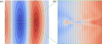
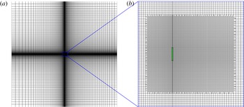
This manuscript presents what we believe is the first attempt to link the two topics, by addressing the stability sensitivity of density-stratified flows. In fact, the sensitivity theory is presented broadly for the Boussinesq equations, with no restriction that the flow in question be density stratified. Nevertheless, we focus our core examples on the stably linearly density-stratified flow around a bluff body (figure 1), so as to highlight core flow features often found in oceanographic flows. By pursuing such examples, we are able not only to replicate sensitivity features found in constant-density flows, but also to reveal previously unseen qualities unique to density-stratified flow physics.
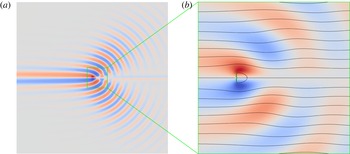
A flow from left to right with a stable, linear, vertical density stratification encounters a vertical thin plate (green) of unit height, at
 $Re=30$
,
 $Fr=1$
and
 $Pr=7.19$
. Colours distinguish the density perturbation from the background stratification (red: positive; blue: negative). (a) The domain
 $[-60,60]\times [-60,60]$
, with exaggerated colours for clarity; the plate is not visible. (b) The domain
 $[-4,12]\times [-8,8]$
, with streamlines also shown.

The essence of linear stability sensitivity theory is to determine the effect of infinitesimal base flow perturbations on the stability of that state. One of the first noteworthy stability sensitivity studies was conducted by Hill (Reference Hill1992), who determined the stability of perturbed base flows. Bottaro, Corbett & Luchini (Reference Bottaro, Corbett and Luchini2003) then examined the effect of base flow velocity perturbations on the stability of parallel flows, via the well-known Orr–Sommerfeld equations. Marquet, Sipp & Jacquin (Reference Marquet, Sipp and Jacquin2008) later built further upon the work of Hill, examining the sensitivity of a cylinder flow. Marquet et al.’s theory calculates the stability perturbations that result from infinitesimal changes in the base flow velocity, or alternatively, from the presence of a steady force.
Simultaneously, Giannetti & Luchini (Reference Giannetti and Luchini2007) presented the sensitivity to spatially localised feedback. In essence, the theory determines the effect that a point feedback mechanism – e.g. by a collocated point actuator and sensor acting under a proportional control law – would have on the flow stability, as a function of the point location in the flow. The most striking result of the sensitivity studies was that the region of high sensitivity in a
 $Re=50$
cylinder flow matched very closely with the loci where a small stationary secondary cylinder suppresses the vortex shedding of the main cylinder (Strykowski & Sreenivasan Reference Strykowski and Sreenivasan1990). In this flow, the base flow sensitivity at
 $Re=46.8$
is qualitatively similar to the sensitivity to spatially localised feedback, albeit with some minor differences. In fact, the two sensitivity calculations are similar, as they are both based on various combinations of the linearised flow operator’s direct and adjoint eigenmodes.
These seminal works paved the way for further developments in the theory and application of stability sensitivity over the last several years. Giannetti, Camarri & Luchini (Reference Giannetti, Camarri and Luchini2010) analysed the secondary instability of the two-dimensional cylinder flow at Reynolds numbers in the low hundreds. Of particular note in the appendix of this work is a profound comment that recirculation regions exhibit particularly high sensitivity to spatially localised feedback. The authors suggest that such a relation can be explained using a local theory. In such an explanation, short-wavelength disturbances are convected by the velocity field, leading to positive feedback mechanisms in recirculation regions where small disturbances can self-amplify and greatly affect the flow stability. The relation between sensitivity and recirculation has also been found in more complex two- and three-dimensional flows (e.g. Fani, Camarri & Salvetti Reference Fani, Camarri and Salvetti2013; Qadri, Mistry & Juniper Reference Qadri, Mistry and Juniper2013; Lashgari et al. Reference Lashgari, Tammisola, Citro, Juniper and Brandt2014; Chen, Rowley & Stone Reference Chen, Rowley and Stone2015). Although we do not pursue the short-wavelength theory, it does motivate us to analyse the stability sensitivity of a bluff-body flow exhibiting recirculation later in this manuscript.
Aside from the aforementioned works, there exist many recent studies applying sensitivity theories to various flows. Instead of listing these in detail, we point out a few alternate techniques that have been developed. Meliga, Pujals & Serre (Reference Meliga, Pujals and Serre2012) successfully applied Marquet et al.’s sensitivity study to a steady force at a high Reynolds number of 13 000, using the global eigenmodes about a mean flow instead of a steady-state flow. Next, Fani et al. (Reference Fani, Camarri and Salvetti2013) studied the flow through a T-shaped mixer and computed the stability sensitivity specifically to the velocity distribution of the inlet. In a shift from the application of sensitivity theories specifically to stability, Meliga et al. (Reference Meliga, Boujo, Pujals and Gallaire2014) studied the sensitivity of a bluff body’s drag force. In addition, Boujo and Gallaire (Reference Boujo and Gallaire2014) examined the sensitivity of features related to flow separation, and applied the theory to the flow over a bump.
The discussion of linear stability and sensitivity theories can be found in a few review articles. Chomaz (Reference Chomaz2005) discusses global stability theory and addresses the role of non-normality and nonlinearity. Luchini & Bottaro (Reference Luchini and Bottaro2014) specifically focus on the role of adjoint equations in stability theory. Finally, Schmid & Brandt (Reference Schmid and Brandt2014) discuss stability, receptivity (as given by adjoint operators) and sensitivity from the general standpoint of optimisation instead of eigendecompositions. Such an approach allows more general discussions of flow systems beyond simple steady states.
At this point, we shift our discussion to density-stratified flows. We focus particularly on stratifications where the background density field is a continuous, monotonically increasing function of displacement in the direction of gravity. These conditions are encountered in oceanographic and atmospheric flows, and form the basis of our computational examples later on. The discussion of stratified flow physics is too expansive to be reviewed here. The basic underlying theory is discussed in the review article by Yih (Reference Yih1969) and the book by Turner (Reference Turner1973). The topic of stratified flow stability is one that deserves mention, but is still too wide of a topic to be reviewed here. The elementary theory is reviewed in the text by Drazin & Reid (Reference Drazin and Reid2004).
Instead, we highlight a few works that provide a context for the application we present. First and foremost, it is well known that inviscid parallel flows with non-zero velocity shear and Richardson number greater than
 $1/4$
(that is, Froude number less than 2) everywhere in the flow are unconditionally stable (Miles Reference Miles1961). Focusing now on non-parallel flows, the topic of the vertical collapse of stratified wakes has been the subject of decades of work (see reviews by Lin & Pao (Reference Lin and Pao1979), Riley & Lelong (Reference Riley and Lelong2000) and Spedding (Reference Spedding2014)). Although the relation between stratified wake collapse and stratified flow stability may not be entirely direct, the former has inspired further research in the latter. For instance, vortices in collapsed stratified turbulent wakes have been shown to exhibit greater persistence, organisation and coherence than in unstratified wakes (Gourlay et al.
Reference Gourlay, Arendt, Fritts and Werne2001).
Somewhat paradoxically, laminar horizontal vortex rings can also exhibit instability and a subsequent collapse in density-stratified flows (van Atta & Hopfinger Reference van Atta and Hopfinger1989; Johari & Fang Reference Johari and Fang1997). Similarly, the zigzag instability of vertical vortex pairs and the subsequent evolution into pancake vortices was reported by Billant & Chomaz (Reference Billant and Chomaz2000) and in subsequent papers. Pancake vortices have since been observed in many different stratified flows, and their stability was studied by Negretti & Billant (Reference Negretti and Billant2013). Boulanger, Meunier & Le Dizès (Reference Boulanger, Meunier and Le Dizès2008) and Candelier, Le Dizès & Millet (Reference Candelier, Le Dizès and Millet2011) respectively examined the instability of a tilted Lamb–Oseen vortex and a tilted Bickley jet in a stratified flow. Le Dizès & Billant (Reference Le Dizès and Billant2009) reported analytical findings specifically on radiative instabilities in stratified flows. Bosco & Meunier (Reference Bosco and Meunier2014) then presented theoretical, experimental and numerical results on the instabilities of stratified wake around a cylinder. Recently, Kaminski, Caulfield & Taylor (Reference Kaminski, Caulfield and Taylor2014) and Ortiz, Donnadieu & Chomaz (Reference Ortiz, Donnadieu and Chomaz2015) respectively analysed the finite-time optimal perturbations of a shear layer and a counter-rotating horizontal vortex pair in a stratified medium.
Again, we do not intend to delve into the details of stratified flow stability, for which there exists a vast literature covering theory, experiments and computations across a wide array of flow conditions. Instead, we merely point out that density stratification can cause complex instabilities that may not be obvious to those more familiar with constant-density flows. These instabilities are the focus of the examples we present later.
In this manuscript, our chief focus is to extend the theory of sensitivity to base flow modifications (Marquet et al. Reference Marquet, Sipp and Jacquin2008) to the Boussinesq equations. The subsequent theory allows us to compute the sensitivity of stability eigenvalues to infinitesimal perturbations in the density or velocity components of base flows. As in Marquet et al. (Reference Marquet, Sipp and Jacquin2008), the sensitivities can be broken down into growth rate and frequency sensitivities. In addition, the construction of the theory reveals the mechanisms by which base flow modifications transport or produce flow perturbations, thereby contributing to the sensitivities.
We demonstrate the theory with a two-dimensional computational example, whereby a flow with a stable linear density stratification encounters a thin plate oriented transversely to the flow (figure 1). In this example, the Reynolds and Prandtl numbers are fixed respectively at 30 and 7.19, and we investigate Froude numbers of 1, 8 and
 $\infty$
.
This manuscript is organised as follows. In § 2, we state the Boussinesq equations and develop the sensitivity to base flow modifications. The computational examples are shown in § 3. Discussions on parallel flow theory, as well as simulations with modified base flows, are presented in § 4. Finally, we summarise the manuscript and provide directions for future work in § 5. The computational methods are described in appendix A and the derivation of an Orr–Sommerfeld-type equation is given in appendix B.
2 Theory
In this section, our primary aim is to present the sensitivity to base flow modifications for the Boussinesq equations. The Boussinesq equations, along with a discussion of the choice of non-dimensionalisation, are presented in § 2.1. The main sensitivity theory, which is presented as partial sensitivities – that is, in terms of partial derivatives – is derived in § 2.2. Finally, in § 2.3, we provide some remarks on how the partial sensitivities could be conceptually combined to form a total sensitivity.
2.1 Boussinesq equations
In this manuscript, we focus specifically on the Boussinesq equations as an approximation of mass and momentum conservation when density fluctuations are suitably small. As in the typical case, we employ the Boussinesq model to simplify the governing equations, with the understanding that they are sufficiently accurate to describe oceanographic and atmospheric flows. Nevertheless, it is obviously the case that many density-varying flows of practical importance cannot be accurately described with the Boussinesq equations. The base flow sensitivity in these situations is a topic reserved for future research.
In the following section, let us assume that variables and operators marked by
 $(\,\tilde{\cdot }\,)$
are dimensional, and all others are non-dimensional. Let
 $\tilde{\boldsymbol{x}}:=\left[\begin{array}{@{}ccc@{}}\tilde{x} & {\tilde{y}} & \tilde{z}\end{array}\right]^{\text{T}}$
and
 $\tilde{t}$
respectively denote displacement and time, and let
 $\tilde{\unicode[STIX]{x1D70C}}(\tilde{\boldsymbol{x}},\tilde{t})$
,
 $\tilde{\boldsymbol{u}}(\tilde{\boldsymbol{x}},\tilde{t}):=\left[\begin{array}{@{}ccc@{}}\tilde{u} (\tilde{\boldsymbol{x}},\tilde{t}) & \tilde{v}(\tilde{\boldsymbol{x}},\tilde{t}) & \tilde{w}(\tilde{\boldsymbol{x}},\tilde{t})\end{array}\right]^{\text{T}}$
and
 $\tilde{p}(\tilde{\boldsymbol{x}},\tilde{t})$
respectively denote the density, velocity and pressure fields. Also, let
 $\tilde{\unicode[STIX]{x1D707}}$
denote the viscosity,
 $\tilde{\unicode[STIX]{x1D6FC}}$
denote the diffusivity of density (which may be, for instance, the effect of thermal conductivity or salinity diffusion),
 $\tilde{\boldsymbol{g}}$
denote the gravitational acceleration vector and
 $\tilde{\unicode[STIX]{x1D70C}}_{c}$
denote a constant density that is characteristic of the entire density field
 $\tilde{\unicode[STIX]{x1D70C}}(\tilde{\boldsymbol{x}},\tilde{t})$
. The dimensional Boussinesq equations we employ are
 $$\begin{eqnarray}\displaystyle \frac{\unicode[STIX]{x2202}}{\unicode[STIX]{x2202}\tilde{t}}\left[\begin{array}{@{}c@{}}\tilde{\unicode[STIX]{x1D70C}}\\ \tilde{\boldsymbol{u}}\end{array}\right]=\left[\begin{array}{@{}c@{}}-\tilde{\boldsymbol{u}}\boldsymbol{\cdot }\tilde{\unicode[STIX]{x1D735}}\tilde{\unicode[STIX]{x1D70C}}+\tilde{\unicode[STIX]{x1D6FC}}\tilde{\unicode[STIX]{x1D6FB}}^{2}\tilde{\unicode[STIX]{x1D70C}}\\ -\tilde{\boldsymbol{u}}\boldsymbol{\cdot }\tilde{\unicode[STIX]{x1D735}}\tilde{\boldsymbol{u}}-{\displaystyle \frac{1}{\tilde{\unicode[STIX]{x1D70C}}_{c}}}\left(\tilde{\unicode[STIX]{x1D735}}\tilde{p}+\tilde{\unicode[STIX]{x1D707}}\tilde{\unicode[STIX]{x1D6FB}}^{2}\tilde{\boldsymbol{u}}+\tilde{\unicode[STIX]{x1D70C}}\tilde{\boldsymbol{g}}\right)\end{array}\right], & & \displaystyle\end{eqnarray}$$
subject to
 $\tilde{\unicode[STIX]{x1D735}}\boldsymbol{\cdot }\tilde{\boldsymbol{u}}=0$
and a problem-dependent set of boundary conditions. This is the form used in most descriptions of stratified flows.
There exist at least two sensible ways to non-dimensionalise these equations. In either case, we begin by selecting some characteristic length scale
 $\tilde{x}_{c}$
, usually determined by the size of some solid body of interest, and some characteristic velocity scale
 $\tilde{u} _{c}$
, usually given by a free-stream flow speed. The non-dimensional parameters associated with these scales are
 $$\begin{eqnarray}\displaystyle \boldsymbol{x}:=\frac{\tilde{\boldsymbol{x}}}{\tilde{x}_{c}},\quad \boldsymbol{u}:=\frac{\tilde{\boldsymbol{u}}}{\tilde{u} _{c}},\quad t:=\frac{\tilde{u} _{c}\tilde{t}}{\tilde{x}_{c}},\quad p:=\frac{\tilde{p}}{\tilde{\unicode[STIX]{x1D70C}}_{c}\tilde{u} _{c}^{2}},\quad Re:=\frac{\tilde{\unicode[STIX]{x1D70C}}_{c}\tilde{x}_{c}\tilde{u} _{c}}{\tilde{\unicode[STIX]{x1D707}}},\quad Pr:=\frac{\tilde{\unicode[STIX]{x1D707}}}{\tilde{\unicode[STIX]{x1D70C}}_{c}\tilde{\unicode[STIX]{x1D6FC}}},\hspace{36.0pt} & & \displaystyle\end{eqnarray}$$
and likewise for
 $x$
,
 $y$
,
 $z$
,
 $u$
,
 $v$
and
 $w$
. The associated operators are
 $$\begin{eqnarray}\displaystyle \unicode[STIX]{x1D735}:=\tilde{x}_{c}\tilde{\unicode[STIX]{x1D735}},\quad \unicode[STIX]{x1D6FB}^{2}:=\unicode[STIX]{x1D735}\boldsymbol{\cdot }\unicode[STIX]{x1D735}=\tilde{x}_{c}^{2}\tilde{\unicode[STIX]{x1D6FB}}^{2}. & & \displaystyle\end{eqnarray}$$
The remaining terms are the density field and gravitational acceleration. If the flow in question is known to be linearly density stratified, then it is typically preferable to non-dimensionalise the density by the background density change
 $\unicode[STIX]{x0394}\tilde{\unicode[STIX]{x1D70C}}\geqslant 0$
that is encountered over a displacement of
 $\tilde{x}_{c}$
, or some other vertical scale, in the direction of gravity (see, e.g. de Stadler, Sarkar & Brucker Reference de Stadler, Sarkar and Brucker2010 and Ortiz et al.
Reference Ortiz, Donnadieu and Chomaz2015). In this framework, the dimensional background density field is
 $$\begin{eqnarray}\displaystyle \tilde{\unicode[STIX]{x1D70C}}_{b}(\tilde{\boldsymbol{x}})=\tilde{\unicode[STIX]{x1D70C}}_{c}-\frac{\unicode[STIX]{x0394}\tilde{\unicode[STIX]{x1D70C}}{\tilde{y}}}{\tilde{x}_{c}}. & & \displaystyle\end{eqnarray}$$
If
 $\tilde{g}:=\Vert \tilde{\boldsymbol{g}}\Vert$
and we define the Brunt–Väisälä frequency (i.e. the characteristic buoyancy frequency) by
 $$\begin{eqnarray}\displaystyle {\tilde{N}}:=\sqrt{\frac{\unicode[STIX]{x0394}\tilde{\unicode[STIX]{x1D70C}}\tilde{g}}{\tilde{\unicode[STIX]{x1D70C}}_{c}\tilde{x}_{c}}}, & & \displaystyle\end{eqnarray}$$
then the Froude number
 $$\begin{eqnarray}\displaystyle Fr:=\frac{\tilde{u} _{c}}{{\tilde{N}}\tilde{x}_{c}}=\tilde{u} _{c}\sqrt{\frac{\tilde{\unicode[STIX]{x1D70C}}_{c}}{\unicode[STIX]{x0394}\tilde{\unicode[STIX]{x1D70C}}\tilde{g}\tilde{x}_{c}}} & & \displaystyle\end{eqnarray}$$
indicates the ratio the buoyancy time scale to the convective time scale in the flow. The limit
 $Fr\rightarrow \infty$
indicates that the flow is unstratified or that gravity is absent.
In this approach, we would define the non-dimensional density
 $$\begin{eqnarray}\displaystyle \unicode[STIX]{x1D70C}_{\unicode[STIX]{x1D6E5}}:=\frac{\tilde{\unicode[STIX]{x1D70C}}}{\unicode[STIX]{x0394}\tilde{\unicode[STIX]{x1D70C}}}. & & \displaystyle\end{eqnarray}$$
The advantage of this non-dimensionalisation is that the Froude number directly appears in the momentum equation, which is written as
 $$\begin{eqnarray}\displaystyle \frac{\unicode[STIX]{x2202}}{\unicode[STIX]{x2202}t}\left[\begin{array}{@{}c@{}}\unicode[STIX]{x1D70C}_{\unicode[STIX]{x1D6E5}}\\ \boldsymbol{u}\end{array}\right]=\left[\begin{array}{@{}c@{}}-\boldsymbol{u}\boldsymbol{\cdot }\unicode[STIX]{x1D735}\unicode[STIX]{x1D70C}_{\unicode[STIX]{x1D6E5}}+{\displaystyle \frac{\unicode[STIX]{x1D6FB}^{2}\unicode[STIX]{x1D70C}_{\unicode[STIX]{x1D6E5}}}{Re\,Pr}}\\ -\boldsymbol{u}\boldsymbol{\cdot }\unicode[STIX]{x1D735}\boldsymbol{u}-\unicode[STIX]{x1D735}p+{\displaystyle \frac{\unicode[STIX]{x1D6FB}^{2}\boldsymbol{u}}{Re}}+{\displaystyle \frac{\unicode[STIX]{x1D70C}_{\unicode[STIX]{x1D6E5}}\boldsymbol{e}_{g}}{Fr^{2}}}\end{array}\right], & & \displaystyle\end{eqnarray}$$
where
 $\boldsymbol{e}_{g}$
is the unit vector in the direction of gravity and the dimensional
 $\tilde{g}$
has been replaced by
 $Fr^{-2}$
(see (6) in de Stadler et al.
Reference de Stadler, Sarkar and Brucker2010). Therefore, the strength of the stratification, which is embodied by
 $Fr$
, is immediately apparent in the resulting non-dimensional Boussinesq equations.
For the purposes of our theoretical development, however, we wish to employ the Boussinesq equations in their general form, without requiring that the background density be linearly stratified. Therefore, we will employ an alternate non-dimensionalisation of density and gravity. This approach affords us broader applicability, at the cost that the equations may be less intuitive in the special case of stratified flows. Let us define
 $$\begin{eqnarray}\displaystyle \unicode[STIX]{x1D70C}:=\frac{\tilde{\unicode[STIX]{x1D70C}}}{\tilde{\unicode[STIX]{x1D70C}}_{c}},\quad \boldsymbol{g}:=\frac{\tilde{x}_{c}\tilde{\boldsymbol{g}}}{\tilde{u} _{c}^{2}}. & & \displaystyle\end{eqnarray}$$
The Boussinesq operator
 $\mathscr{N}$
and associated partial differential equation then become
 $$\begin{eqnarray}\displaystyle \frac{\unicode[STIX]{x2202}}{\unicode[STIX]{x2202}t}\left[\begin{array}{@{}c@{}}\unicode[STIX]{x1D70C}\\ \boldsymbol{u}\end{array}\right]=\mathscr{N}\left(\left[\begin{array}{@{}c@{}}\unicode[STIX]{x1D70C}\\ \boldsymbol{u}\end{array}\right]\right):=\left[\begin{array}{@{}c@{}}-\boldsymbol{u}\boldsymbol{\cdot }\unicode[STIX]{x1D735}\unicode[STIX]{x1D70C}+{\displaystyle \frac{\unicode[STIX]{x1D6FB}^{2}\unicode[STIX]{x1D70C}}{Re\,Pr}}\\ -\boldsymbol{u}\boldsymbol{\cdot }\unicode[STIX]{x1D735}\boldsymbol{u}-\unicode[STIX]{x1D735}p+{\displaystyle \frac{\unicode[STIX]{x1D6FB}^{2}\boldsymbol{u}}{Re}}+\unicode[STIX]{x1D70C}\boldsymbol{g}\end{array}\right], & & \displaystyle\end{eqnarray}$$
subject to
 $\unicode[STIX]{x1D735}\boldsymbol{\cdot }\boldsymbol{u}=0$
and a problem-dependent set of boundary conditions.
If we do suppose that the flow in question is stably linearly stratified, then we define
 $g:=\Vert \boldsymbol{g}\Vert$
and set
 $\unicode[STIX]{x0394}\unicode[STIX]{x1D70C}:=\unicode[STIX]{x0394}\tilde{\unicode[STIX]{x1D70C}}/\tilde{\unicode[STIX]{x1D70C}}_{c}\geqslant 0$
as the background density change over a displacement of one non-dimensional unit in the direction of gravity. The Froude number (2.6) is then
 $$\begin{eqnarray}\displaystyle Fr=\frac{1}{\sqrt{\unicode[STIX]{x0394}\unicode[STIX]{x1D70C}g}}. & & \displaystyle\end{eqnarray}$$
In this formulation, the choice of
 $\unicode[STIX]{x0394}\unicode[STIX]{x1D70C}$
and
 $g$
for a given
 $Fr$
is admittedly somewhat ambiguous. An examination of (2.10) reveals that
 $\unicode[STIX]{x1D70C}$
and
 $g$
can be freely scaled inversely proportionally to each other, with no effect on
 $\boldsymbol{u}$
. How, then, should the Froude number be set? In the stratification-based non-dimensionalisation (2.7), (2.8), some authors fix the density scale while varying gravity (e.g. de Stadler et al.
Reference de Stadler, Sarkar and Brucker2010). We choose to do the opposite, which is to fix
 $g$
but vary the
 $\unicode[STIX]{x0394}\unicode[STIX]{x1D70C}$
scale. This approach is more physically intuitive, since in reality, the
 $Fr=\infty$
case is more accurately an absence of stratification than an absence of gravity. The choice of density scaling will have an effect on the inner product over infinitesimal fields to be used later (2.14).
To enable the use of linear stability theory, we will assume that there exists a steady state
 $\left[\begin{array}{@{}cc@{}}\unicode[STIX]{x1D70C}_{0}(\boldsymbol{x}) & \boldsymbol{u}_{0}^{\text{T}}(\boldsymbol{x})\end{array}\right]^{\text{T}}$
, with
 $\unicode[STIX]{x1D735}\boldsymbol{\cdot }\boldsymbol{u}_{0}=0$
, such that
 $$\begin{eqnarray}\displaystyle \mathscr{N}\left(\left[\begin{array}{@{}c@{}}\unicode[STIX]{x1D70C}_{0}(\boldsymbol{x})\\ \boldsymbol{u}_{0}(\boldsymbol{x})\end{array}\right]\right)=\left[\begin{array}{@{}c@{}}-\boldsymbol{u}_{0}\boldsymbol{\cdot }\unicode[STIX]{x1D735}\unicode[STIX]{x1D70C}_{0}+{\displaystyle \frac{\unicode[STIX]{x1D6FB}^{2}\unicode[STIX]{x1D70C}_{0}}{Re\,Pr}}\\ -\boldsymbol{u}_{0}\boldsymbol{\cdot }\unicode[STIX]{x1D735}\boldsymbol{u}_{0}-\unicode[STIX]{x1D735}p_{0}+{\displaystyle \frac{\unicode[STIX]{x1D6FB}^{2}\boldsymbol{u}_{0}}{Re}}+\unicode[STIX]{x1D70C}_{0}\boldsymbol{g}\end{array}\right]=\mathbf{0}. & & \displaystyle\end{eqnarray}$$
Next, we suppose that
 $\unicode[STIX]{x1D70C}^{\prime }(\boldsymbol{x},t)$
,
 $\boldsymbol{u}^{\prime }(\boldsymbol{x},t):=\left[\begin{array}{@{}ccc@{}}u^{\prime }(\boldsymbol{x},t) & v^{\prime }(\boldsymbol{x},t) & w^{\prime }(\boldsymbol{x},t)\end{array}\right]^{\text{T}}$
, and
 $p^{\prime }(\boldsymbol{x},t)$
are infinitesimal complex-valued perturbations in density, velocity and pressure from the steady-state solution. The linearisation of (2.10) about
 $\left[\begin{array}{@{}cc@{}}\unicode[STIX]{x1D70C}_{0}(\boldsymbol{x}) & \boldsymbol{u}_{0}^{\text{T}}(\boldsymbol{x})\end{array}\right]^{\text{T}}$
is then given by the linear operator
 $\mathscr{L}$
and the associated partial differential equation
 $$\begin{eqnarray}\displaystyle \frac{\unicode[STIX]{x2202}}{\unicode[STIX]{x2202}t}\left[\begin{array}{@{}c@{}}\unicode[STIX]{x1D70C}^{\prime }\\ \boldsymbol{u}^{\prime }\end{array}\right]=\mathscr{L}\left[\begin{array}{@{}c@{}}\unicode[STIX]{x1D70C}^{\prime }\\ \boldsymbol{u}^{\prime }\end{array}\right]:=\left[\begin{array}{@{}c@{}}-\boldsymbol{u}_{0}\boldsymbol{\cdot }\unicode[STIX]{x1D735}\unicode[STIX]{x1D70C}^{\prime }-\boldsymbol{u}^{\prime }\boldsymbol{\cdot }\unicode[STIX]{x1D735}\unicode[STIX]{x1D70C}_{0}+{\displaystyle \frac{\unicode[STIX]{x1D6FB}^{2}\unicode[STIX]{x1D70C}^{\prime }}{Re\,Pr}}\\ -\boldsymbol{u}_{0}\boldsymbol{\cdot }\unicode[STIX]{x1D735}\boldsymbol{u}^{\prime }-\boldsymbol{u}^{\prime }\boldsymbol{\cdot }\unicode[STIX]{x1D735}\boldsymbol{u}_{0}-\unicode[STIX]{x1D735}p^{\prime }+{\displaystyle \frac{\unicode[STIX]{x1D6FB}^{2}\boldsymbol{u}^{\prime }}{Re}}+\unicode[STIX]{x1D70C}^{\prime }\boldsymbol{g}\end{array}\right], & & \displaystyle\end{eqnarray}$$
subject to
 $\unicode[STIX]{x1D735}\boldsymbol{\cdot }\boldsymbol{u}^{\prime }=0$
. The boundary conditions for (2.13) are typically the homogeneous versions of the conditions on
 $\mathscr{N}$
(2.10), since
 $\left[\begin{array}{@{}cc@{}}\unicode[STIX]{x1D70C}_{0}+\unicode[STIX]{x1D70C}^{\prime } & (\boldsymbol{u}_{0}+\boldsymbol{u}^{\prime })^{\text{T}}\end{array}\right]^{\text{T}}$
must satisfy the same boundary conditions as
 $\left[\begin{array}{@{}cc@{}}\unicode[STIX]{x1D70C}_{0} & \boldsymbol{u}_{0}^{\text{T}}\end{array}\right]^{\text{T}}$
.
It is typically convenient to define an adjoint linear operator with respect to some inner product, so as to enable the computation of various types of sensitivity. For complex-valued density perturbations
 $\unicode[STIX]{x1D70C}^{\prime }$
,
 $\hat{\unicode[STIX]{x1D70C}}^{\prime }$
and velocity perturbations
 $\boldsymbol{u}^{\prime }$
,
 $\hat{\boldsymbol{u}}^{\prime }:=\left[\begin{array}{@{}ccc@{}}\hat{u} ^{\prime } & \hat{v}^{\prime } & {\hat{w}}^{\prime }\end{array}\right]^{\text{T}}$
in some control volume
 $\unicode[STIX]{x1D6FA}$
, along with the complex conjugation operation
 $(\bar{\cdot })$
, we choose the inner product
 $$\begin{eqnarray}\displaystyle \left<\left[\begin{array}{@{}c@{}}\unicode[STIX]{x1D70C}^{\prime }\\ \boldsymbol{u}^{\prime }\end{array}\right],\left[\begin{array}{@{}c@{}}\hat{\unicode[STIX]{x1D70C}}^{\prime }\\ \hat{\boldsymbol{u}}^{\prime }\end{array}\right]\right>:=\int _{\unicode[STIX]{x1D6FA}}(\unicode[STIX]{x1D70C}^{\prime }\bar{\hat{\unicode[STIX]{x1D70C}}}^{\prime }+\boldsymbol{u}^{\prime }\boldsymbol{\cdot }\bar{\hat{\boldsymbol{u}}}^{\prime })\,\text{d}V. & & \displaystyle\end{eqnarray}$$
We remark that the weighting of the density and velocity terms in the above integral is arbitrary. Nevertheless, we do not introduce any additional weighting, for convenience.
The adjoint linear operator
 $\mathscr{L}^{\ast }$
is then defined as the operator – with an appropriate set of boundary conditions – that satisfies
 $$\begin{eqnarray}\displaystyle \left<\mathscr{L}\left[\begin{array}{@{}c@{}}\unicode[STIX]{x1D70C}^{\prime }\\ \boldsymbol{u}^{\prime }\end{array}\right],\left[\begin{array}{@{}c@{}}\hat{\unicode[STIX]{x1D70C}}^{\prime }\\ \hat{\boldsymbol{u}}^{\prime }\end{array}\right]\right>=\left<\left[\begin{array}{@{}c@{}}\unicode[STIX]{x1D70C}^{\prime }\\ \boldsymbol{u}^{\prime }\end{array}\right],\mathscr{L}^{\ast }\left[\begin{array}{@{}c@{}}\hat{\unicode[STIX]{x1D70C}}^{\prime }\\ \hat{\boldsymbol{u}}^{\prime }\end{array}\right]\right>. & & \displaystyle\end{eqnarray}$$
For
 $\hat{\unicode[STIX]{x1D70C}}^{\prime }$
,
 $\hat{\boldsymbol{u}}^{\prime }$
and the adjoint linearised pressure
 $\hat{p}^{\prime }$
, this adjoint operator is given by
 $$\begin{eqnarray}\displaystyle \mathscr{L}^{\ast }\left[\begin{array}{@{}c@{}}\hat{\unicode[STIX]{x1D70C}}^{\prime }\\ \hat{\boldsymbol{u}}^{\prime }\end{array}\right]=\left[\begin{array}{@{}c@{}}\boldsymbol{u}_{0}\boldsymbol{\cdot }\unicode[STIX]{x1D735}\hat{\unicode[STIX]{x1D70C}}^{\prime }+{\displaystyle \frac{\unicode[STIX]{x1D6FB}^{2}\hat{\unicode[STIX]{x1D70C}}^{\prime }}{Re\,Pr}}+\boldsymbol{g}\boldsymbol{\cdot }\hat{\boldsymbol{u}}^{\prime }\\ -\hat{\unicode[STIX]{x1D70C}}^{\prime }\unicode[STIX]{x1D735}\unicode[STIX]{x1D70C}_{0}-(\unicode[STIX]{x1D735}\boldsymbol{u}_{0})\boldsymbol{\cdot }\hat{\boldsymbol{u}}^{\prime }+\boldsymbol{u}_{0}\boldsymbol{\cdot }\unicode[STIX]{x1D735}\hat{\boldsymbol{u}}^{\prime }-\unicode[STIX]{x1D735}\hat{p}^{\prime }+{\displaystyle \frac{\unicode[STIX]{x1D6FB}^{2}\hat{\boldsymbol{u}}^{\prime }}{Re}}\end{array}\right], & & \displaystyle\end{eqnarray}$$
subject to
 $\unicode[STIX]{x1D735}\boldsymbol{\cdot }\hat{\boldsymbol{u}}^{\prime }=0$
(see (21) in Ortiz et al.
Reference Ortiz, Donnadieu and Chomaz2015). To clarify the notation, for two vector fields
 $\boldsymbol{u}$
and
 $\boldsymbol{v}$
given respectively in indicial notation by
 $u_{i}$
and
 $v_{i}$
,
 $((\unicode[STIX]{x1D735}\boldsymbol{u})\boldsymbol{\cdot }\boldsymbol{v})_{i}=(\unicode[STIX]{x2202}u_{j}/\unicode[STIX]{x2202}x_{i})v_{j}$
. Given
 $$\begin{eqnarray}\displaystyle \boldsymbol{J} & := & \displaystyle -(\unicode[STIX]{x1D70C}^{\prime }\bar{\hat{\unicode[STIX]{x1D70C}}}^{\prime }+\boldsymbol{u}^{\prime }\boldsymbol{\cdot }\bar{\hat{\boldsymbol{u}}}^{\prime })\boldsymbol{u}_{0}-p^{\prime }\bar{\hat{\boldsymbol{u}}}^{\prime }+\bar{\hat{p}}^{\prime }\boldsymbol{u}^{\prime }\nonumber\\ \displaystyle & & \displaystyle +\,\frac{1}{Re}\left(\frac{1}{Pr}\left(\bar{\hat{\unicode[STIX]{x1D70C}}}^{\prime }\unicode[STIX]{x1D735}\unicode[STIX]{x1D70C}^{\prime }-\unicode[STIX]{x1D70C}^{\prime }\unicode[STIX]{x1D735}\bar{\hat{\unicode[STIX]{x1D70C}}}^{\prime }\right)+(\unicode[STIX]{x1D735}\boldsymbol{u}^{\prime })\boldsymbol{\cdot }\bar{\hat{\boldsymbol{u}}}^{\prime }-(\unicode[STIX]{x1D735}\bar{\hat{\boldsymbol{u}}}^{\prime })\boldsymbol{\cdot }\boldsymbol{u}^{\prime }\right),\end{eqnarray}$$
and the outward normal vector
 $\boldsymbol{n}$
on the boundary
 $\unicode[STIX]{x2202}\unicode[STIX]{x1D6FA}$
of the control volume
 $\unicode[STIX]{x1D6FA}$
, the boundary condition on
 $\unicode[STIX]{x2202}\unicode[STIX]{x1D6FA}$
associated with
 $\mathscr{L}^{\ast }$
is
 $$\begin{eqnarray}\displaystyle \boldsymbol{J}\boldsymbol{\cdot }\boldsymbol{n}=0. & & \displaystyle\end{eqnarray}$$
The associated adjoint linearised Boussinesq equations are simply
 $$\begin{eqnarray}\displaystyle \frac{\unicode[STIX]{x2202}}{\unicode[STIX]{x2202}t}\left[\begin{array}{@{}c@{}}\hat{\unicode[STIX]{x1D70C}}^{\prime }\\ \hat{\boldsymbol{u}}^{\prime }\end{array}\right]=\mathscr{L}^{\ast }\left[\begin{array}{@{}c@{}}\hat{\unicode[STIX]{x1D70C}}^{\prime }\\ \hat{\boldsymbol{u}}^{\prime }\end{array}\right]. & & \displaystyle\end{eqnarray}$$
The adjoint is commonly derived using a bilinear concomitant (see Schmid & Henningson Reference Schmid and Henningson2001; Giannetti & Luchini Reference Giannetti and Luchini2007), but it can be verified perhaps more intuitively from (2.15) itself. In summary, it can be shown that
 $$\begin{eqnarray}\displaystyle \left(\mathscr{L}\left[\begin{array}{@{}c@{}}\unicode[STIX]{x1D70C}^{\prime }\\ \boldsymbol{u}^{\prime }\end{array}\right]\right)\boldsymbol{\cdot }\overline{\left[\begin{array}{@{}c@{}}\hat{\unicode[STIX]{x1D70C}}^{\prime }\\ \hat{\boldsymbol{u}}^{\prime }\end{array}\right]}=\left[\begin{array}{@{}c@{}}\unicode[STIX]{x1D70C}^{\prime }\\ \boldsymbol{u}^{\prime }\end{array}\right]\boldsymbol{\cdot }\overline{\mathscr{L}^{\ast }\left[\begin{array}{@{}c@{}}\hat{\unicode[STIX]{x1D70C}}^{\prime }\\ \hat{\boldsymbol{u}}^{\prime }\end{array}\right]}+\unicode[STIX]{x1D735}\boldsymbol{\cdot }\boldsymbol{J}. & & \displaystyle\end{eqnarray}$$
Integrating (2.20) over
 $\unicode[STIX]{x1D6FA}$
and applying the divergence theorem, we find that
 $$\begin{eqnarray}\displaystyle \left<\mathscr{L}\left[\begin{array}{@{}c@{}}\unicode[STIX]{x1D70C}^{\prime }\\ \boldsymbol{u}^{\prime }\end{array}\right],\left[\begin{array}{@{}c@{}}\hat{\unicode[STIX]{x1D70C}}^{\prime }\\ \hat{\boldsymbol{u}}^{\prime }\end{array}\right]\right>=\left<\left[\begin{array}{@{}c@{}}\unicode[STIX]{x1D70C}^{\prime }\\ \boldsymbol{u}^{\prime }\end{array}\right],\mathscr{L}^{\ast }\left[\begin{array}{@{}c@{}}\hat{\unicode[STIX]{x1D70C}}^{\prime }\\ \hat{\boldsymbol{u}}^{\prime }\end{array}\right]\right>+\oint _{\unicode[STIX]{x2202}\unicode[STIX]{x1D6FA}}\boldsymbol{J}\boldsymbol{\cdot }\boldsymbol{n}\,\text{d}S. & & \displaystyle\end{eqnarray}$$
Hence, (2.16) and (2.18) are sufficient conditions for the adjoint relation (2.15) to be satisfied.
2.2 Sensitivity to base flow modifications
The crux of linear stability theory is that the eigendecomposition of the linearised dynamics (2.13) reveals the stability characteristics of the steady-state flow. The Hartman–Grobman theorem states that the nonlinear (2.10) and linearised (2.13) dynamics will have the same stability at the fixed point
 $\left[\begin{array}{@{}cc@{}}\unicode[STIX]{x1D70C}_{0} & \boldsymbol{u}_{0}^{\text{T}}\end{array}\right]^{\text{T}}$
, so long as none of the eigenvalues have a zero real part. We remind that the theorem makes no implications about the size of the domain of attraction in the nonlinear dynamics, nor does the linear stability analysis necessarily reveal finite-time transient growths stemming from the non-normality of
 $\mathscr{L}$
. The topics of nonlinear and non-normal stability are discussed in works by Schmid & Henningson (Reference Schmid and Henningson2001), Chomaz (Reference Chomaz2005) and Schmid & Brandt (Reference Schmid and Brandt2014), among others.
The sensitivity of the stability to base flow modifications, as presented by Marquet et al. (Reference Marquet, Sipp and Jacquin2008), provides an elegant closed-form solution for the eigenvalue perturbation resulting from an infinitesimal base flow perturbation. The direct and adjoint eigenmodes can be combined to construct a sensitivity field, which yields the eigenvalue perturbation via an inner product with the base flow perturbation. Whereas Marquet et al. presented the theory for constant-density flows, we now expand this theory to the Boussinesq equations, for which we assume that the density field is not constant, but is still close to a characteristic value. We will see that certain terms from Marquet et al.’s theory will remain, but additional terms stemming from the density field will appear as well.
In our notation, we will express the direct and adjoint eigendecompositions respectively as
 $$\begin{eqnarray}\displaystyle & \displaystyle \mathscr{L}\unicode[STIX]{x1D753}=\unicode[STIX]{x1D706}\unicode[STIX]{x1D753}, & \displaystyle\end{eqnarray}$$
 $$\begin{eqnarray}\displaystyle & \displaystyle \mathscr{L}^{\ast }\unicode[STIX]{x1D74D}=\bar{\unicode[STIX]{x1D706}}\unicode[STIX]{x1D74D}. & \displaystyle\end{eqnarray}$$
 $$\begin{eqnarray}\displaystyle \unicode[STIX]{x1D753}=\left[\begin{array}{@{}c@{}}\unicode[STIX]{x1D719}_{\unicode[STIX]{x1D70C}}\\ \unicode[STIX]{x1D753}_{\boldsymbol{u}}\end{array}\right],\quad \unicode[STIX]{x1D74D}=\left[\begin{array}{@{}c@{}}\unicode[STIX]{x1D713}_{\unicode[STIX]{x1D70C}}\\ \unicode[STIX]{x1D74D}_{\boldsymbol{u}}\end{array}\right], & & \displaystyle\end{eqnarray}$$
with the
 $\unicode[STIX]{x1D70C}$
subscript indicating the density component and the
 $\boldsymbol{u}$
subscript indicating the velocity component. Note that based on the definitions of the linear operators,
 $\unicode[STIX]{x1D735}\boldsymbol{\cdot }\unicode[STIX]{x1D753}_{\boldsymbol{u}}=\unicode[STIX]{x1D735}\boldsymbol{\cdot }\unicode[STIX]{x1D74D}_{\boldsymbol{u}}=0$
. As usual, the eigenvalues
 $\unicode[STIX]{x1D706}$
are the complex scalars that satisfy (2.22); if
 $\unicode[STIX]{x1D753}$
is the initial condition to a linearised flow, then the solution of the flow is given by
 $\text{e}^{\unicode[STIX]{x1D706}t}\unicode[STIX]{x1D753}$
. Through our notation, we imply that the above equations hold for all eigenvalue–eigenmode pairs, and we leave out eigenvalue–eigenmode indices for brevity.
As in previous works (e.g. Giannetti & Luchini Reference Giannetti and Luchini2007), the sensitivity analysis essentially computes what eigenvalue perturbation
 $\unicode[STIX]{x1D6FF}\unicode[STIX]{x1D706}$
would result from an infinitesimal perturbation in the linearised dynamics
 $\unicode[STIX]{x1D6FF}\mathscr{L}$
. Without making any assumptions on
 $\unicode[STIX]{x1D6FF}\mathscr{L}$
besides its infinitesimal scale, a perturbation in (2.22a
) yields
 $$\begin{eqnarray}\displaystyle \unicode[STIX]{x1D6FF}\mathscr{L}\unicode[STIX]{x1D753}+\mathscr{L}\unicode[STIX]{x1D6FF}\unicode[STIX]{x1D753}=\unicode[STIX]{x1D6FF}\unicode[STIX]{x1D706}\unicode[STIX]{x1D753}+\unicode[STIX]{x1D706}\unicode[STIX]{x1D6FF}\unicode[STIX]{x1D753}. & & \displaystyle\end{eqnarray}$$
In this form, we have not set
 $\unicode[STIX]{x1D6FF}\mathscr{L}$
yet, so we cannot compute
 $\unicode[STIX]{x1D6FF}\unicode[STIX]{x1D753}$
at this point. We can compute
 $\unicode[STIX]{x1D6FF}\unicode[STIX]{x1D706}$
without computing
 $\unicode[STIX]{x1D6FF}\unicode[STIX]{x1D753}$
, however, by taking the inner product of (2.24) with
 $\unicode[STIX]{x1D74D}$
. Noting that
 $$\begin{eqnarray}\displaystyle \left<\mathscr{L}\unicode[STIX]{x1D6FF}\unicode[STIX]{x1D753},\unicode[STIX]{x1D74D}\right>=\left<\unicode[STIX]{x1D6FF}\unicode[STIX]{x1D753},\mathscr{L}^{\ast }\unicode[STIX]{x1D74D}\right>=\left<\unicode[STIX]{x1D6FF}\unicode[STIX]{x1D753},\bar{\unicode[STIX]{x1D706}}\unicode[STIX]{x1D74D}\right>=\left<\unicode[STIX]{x1D706}\unicode[STIX]{x1D6FF}\unicode[STIX]{x1D753},\unicode[STIX]{x1D74D}\right>, & & \displaystyle\end{eqnarray}$$
(2.24) conveniently reduces to
 $\left<\unicode[STIX]{x1D6FF}\mathscr{L}\unicode[STIX]{x1D753},\unicode[STIX]{x1D74D}\right>=\left<\unicode[STIX]{x1D6FF}\unicode[STIX]{x1D706}\unicode[STIX]{x1D753},\unicode[STIX]{x1D74D}\right>$
, that is,
 $$\begin{eqnarray}\displaystyle \unicode[STIX]{x1D6FF}\unicode[STIX]{x1D706}=\frac{\left<\unicode[STIX]{x1D6FF}\mathscr{L}\unicode[STIX]{x1D753},\unicode[STIX]{x1D74D}\right>}{\left<\unicode[STIX]{x1D753},\unicode[STIX]{x1D74D}\right>}. & & \displaystyle\end{eqnarray}$$
This equation forms the basis of stability sensitivity analyses; all that remains is to choose
 $\unicode[STIX]{x1D6FF}\mathscr{L}$
.
In the spirit of Marquet et al. (Reference Marquet, Sipp and Jacquin2008), we will define
 $\unicode[STIX]{x1D6FF}\mathscr{L}$
to be the change in the linearised dynamics resulting from an infinitesimal change in the base flow. We will primarily consider two cases: a change in the base density field
 $\unicode[STIX]{x1D70C}_{0}(\boldsymbol{x})$
with a fixed base velocity field
 $\boldsymbol{u}_{0}(\boldsymbol{x})$
, and a change in
 $\boldsymbol{u}_{0}(\boldsymbol{x})$
with a fixed
 $\unicode[STIX]{x1D70C}_{0}(\boldsymbol{x})$
. In § 2.3, we provide some remarks that tie these two cases together.
In the former case, it is apparent from the linearised dynamics (2.13) that if the base flow density changes infinitesimally from
 $\unicode[STIX]{x1D70C}_{0}(\boldsymbol{x})$
to
 $\unicode[STIX]{x1D70C}_{0}(\boldsymbol{x})+\unicode[STIX]{x1D6FF}\unicode[STIX]{x1D70C}_{0}(\boldsymbol{x})$
, then the corresponding change in the linearised dynamics is
 $$\begin{eqnarray}\displaystyle \unicode[STIX]{x1D6FF}\mathscr{L}\left[\begin{array}{@{}c@{}}\unicode[STIX]{x1D70C}^{\prime }\\ \boldsymbol{u}^{\prime }\end{array}\right]=\left[\begin{array}{@{}c@{}}-\boldsymbol{u}^{\prime }\boldsymbol{\cdot }\unicode[STIX]{x1D735}\unicode[STIX]{x1D6FF}\unicode[STIX]{x1D70C}_{0}\\ \mathbf{0}\end{array}\right]. & & \displaystyle\end{eqnarray}$$
Defining the inner product
 $$\begin{eqnarray}\displaystyle \left<\unicode[STIX]{x1D70C}^{\prime },\hat{\unicode[STIX]{x1D70C}}^{\prime }\right>:=\int _{\unicode[STIX]{x1D6FA}}\unicode[STIX]{x1D70C}^{\prime }\bar{\hat{\unicode[STIX]{x1D70C}}}^{\prime }\,\text{d}V & & \displaystyle\end{eqnarray}$$
for scalar fields, we follow (2.26) and find that the corresponding eigenvalue shift is
 $$\begin{eqnarray}\displaystyle \unicode[STIX]{x1D6FF}\unicode[STIX]{x1D706}=\frac{\left<-\unicode[STIX]{x1D753}_{\boldsymbol{u}}\boldsymbol{\cdot }\unicode[STIX]{x1D735}\unicode[STIX]{x1D6FF}\unicode[STIX]{x1D70C}_{0},\unicode[STIX]{x1D713}_{\unicode[STIX]{x1D70C}}\right>}{\left<\unicode[STIX]{x1D753},\unicode[STIX]{x1D74D}\right>}. & & \displaystyle\end{eqnarray}$$
It is more convenient and elegant to express the above as an inner product of some quantity with
 $\unicode[STIX]{x1D6FF}\unicode[STIX]{x1D70C}_{0}$
, so as to clarify the relation between
 $\unicode[STIX]{x1D6FF}\unicode[STIX]{x1D70C}_{0}$
and
 $\unicode[STIX]{x1D6FF}\unicode[STIX]{x1D706}$
. Using integration by parts, we obtain
 $$\begin{eqnarray}\displaystyle \displaystyle \unicode[STIX]{x1D6FF}\unicode[STIX]{x1D706} & = & \displaystyle \displaystyle \frac{1}{\left<\unicode[STIX]{x1D753},\unicode[STIX]{x1D74D}\right>}\int _{\unicode[STIX]{x1D6FA}}-\bar{\unicode[STIX]{x1D713}}_{\unicode[STIX]{x1D70C}}\unicode[STIX]{x1D753}_{\boldsymbol{u}}\boldsymbol{\cdot }\unicode[STIX]{x1D735}\unicode[STIX]{x1D6FF}\unicode[STIX]{x1D70C}_{0}\,\text{d}V\end{eqnarray}$$
 $$\begin{eqnarray}\displaystyle & = & \displaystyle \displaystyle \frac{1}{\left<\unicode[STIX]{x1D753},\unicode[STIX]{x1D74D}\right>}\left(\int _{\unicode[STIX]{x1D6FA}}\unicode[STIX]{x1D6FF}\unicode[STIX]{x1D70C}_{0}\unicode[STIX]{x1D753}_{\boldsymbol{u}}\boldsymbol{\cdot }\unicode[STIX]{x1D735}\bar{\unicode[STIX]{x1D713}}_{\unicode[STIX]{x1D70C}}\,\text{d}V-\oint _{\unicode[STIX]{x2202}\unicode[STIX]{x1D6FA}}\unicode[STIX]{x1D6FF}\unicode[STIX]{x1D70C}_{0}\bar{\unicode[STIX]{x1D713}}_{\unicode[STIX]{x1D70C}}\unicode[STIX]{x1D753}_{\boldsymbol{u}}\boldsymbol{\cdot }\boldsymbol{n}\,\text{d}S\right),\end{eqnarray}$$
 $\unicode[STIX]{x1D735}\boldsymbol{\cdot }\unicode[STIX]{x1D753}_{\boldsymbol{u}}=0$
. Let us consider the physically realistic case that
 $\unicode[STIX]{x1D6FF}\unicode[STIX]{x1D70C}_{0}$
is real valued, and assume the boundary condition that
 $$\begin{eqnarray}\displaystyle \unicode[STIX]{x1D6FF}\unicode[STIX]{x1D70C}_{0}\bar{\unicode[STIX]{x1D713}}_{\unicode[STIX]{x1D70C}}\unicode[STIX]{x1D753}_{\boldsymbol{u}}\boldsymbol{\cdot }\boldsymbol{n}=0 & & \displaystyle\end{eqnarray}$$
on
 $\unicode[STIX]{x2202}\unicode[STIX]{x1D6FA}$
. Then, we can define the partial sensitivity to base flow density modifications
 $$\begin{eqnarray}\displaystyle \frac{\unicode[STIX]{x2202}\unicode[STIX]{x1D706}}{\unicode[STIX]{x2202}\unicode[STIX]{x1D70C}_{0}}:=\frac{\unicode[STIX]{x1D753}_{\boldsymbol{u}}\boldsymbol{\cdot }\unicode[STIX]{x1D735}\bar{\unicode[STIX]{x1D713}}_{\unicode[STIX]{x1D70C}}}{\left<\unicode[STIX]{x1D753},\unicode[STIX]{x1D74D}\right>}, & & \displaystyle\end{eqnarray}$$
so that the eigenvalue shift is conveniently expressed as
 $$\begin{eqnarray}\displaystyle \unicode[STIX]{x1D6FF}\unicode[STIX]{x1D706}=\left<\frac{\unicode[STIX]{x2202}\unicode[STIX]{x1D706}}{\unicode[STIX]{x2202}\unicode[STIX]{x1D70C}_{0}},\unicode[STIX]{x1D6FF}\unicode[STIX]{x1D70C}_{0}\right>. & & \displaystyle\end{eqnarray}$$
We specifically denote (2.32) as a partial sensitivity, because we have assumed that the base flow velocity field
 $\boldsymbol{u}_{0}$
is unchanged.
Next, we can perform the same analysis for the case where
 $\boldsymbol{u}_{0}$
undergoes an infinitesimal shift
 $\unicode[STIX]{x1D6FF}\boldsymbol{u}_{0}$
, but
 $\unicode[STIX]{x1D70C}_{0}$
remains unchanged. In this case, the corresponding shift in the linearised dynamics (2.13) is
 $$\begin{eqnarray}\displaystyle \unicode[STIX]{x1D6FF}\mathscr{L}\left[\begin{array}{@{}c@{}}\unicode[STIX]{x1D70C}^{\prime }\\ \boldsymbol{u}^{\prime }\end{array}\right]=\left[\begin{array}{@{}c@{}}-\unicode[STIX]{x1D6FF}\boldsymbol{u}_{0}\boldsymbol{\cdot }\unicode[STIX]{x1D735}\unicode[STIX]{x1D70C}^{\prime }\\ -\unicode[STIX]{x1D6FF}\boldsymbol{u}_{0}\boldsymbol{\cdot }\unicode[STIX]{x1D735}\boldsymbol{u}^{\prime }-\boldsymbol{u}^{\prime }\boldsymbol{\cdot }\unicode[STIX]{x1D735}\unicode[STIX]{x1D6FF}\boldsymbol{u}_{0}\end{array}\right]. & & \displaystyle\end{eqnarray}$$
Following (2.26), the resulting eigenvalue shift is
 $$\begin{eqnarray}\displaystyle \unicode[STIX]{x1D6FF}\unicode[STIX]{x1D706}=\frac{1}{\left<\unicode[STIX]{x1D753},\unicode[STIX]{x1D74D}\right>}\int _{\unicode[STIX]{x1D6FA}}\left(-\bar{\unicode[STIX]{x1D713}}_{\unicode[STIX]{x1D70C}}\unicode[STIX]{x1D6FF}\boldsymbol{u}_{0}\boldsymbol{\cdot }\unicode[STIX]{x1D735}\unicode[STIX]{x1D719}_{\unicode[STIX]{x1D70C}}-(\unicode[STIX]{x1D6FF}\boldsymbol{u}_{0}\boldsymbol{\cdot }\unicode[STIX]{x1D735}\unicode[STIX]{x1D753}_{\boldsymbol{u}})\boldsymbol{\cdot }\bar{\unicode[STIX]{x1D74D}}_{\boldsymbol{u}}-(\unicode[STIX]{x1D753}_{\boldsymbol{u}}\boldsymbol{\cdot }\unicode[STIX]{x1D735}\unicode[STIX]{x1D6FF}\boldsymbol{u}_{0})\boldsymbol{\cdot }\bar{\unicode[STIX]{x1D74D}}_{\boldsymbol{u}}\right)\,\text{d}V. & & \displaystyle\end{eqnarray}$$
Integration by parts on the last summand of the integrand yields
 $$\begin{eqnarray}\displaystyle \int _{\unicode[STIX]{x1D6FA}}-(\unicode[STIX]{x1D753}_{\boldsymbol{u}}\boldsymbol{\cdot }\unicode[STIX]{x1D735}\unicode[STIX]{x1D6FF}\boldsymbol{u}_{0})\boldsymbol{\cdot }\bar{\unicode[STIX]{x1D74D}}_{\boldsymbol{u}}\,\text{d}V=\int _{\unicode[STIX]{x1D6FA}}(\unicode[STIX]{x1D753}_{\boldsymbol{u}}\boldsymbol{\cdot }\unicode[STIX]{x1D735}\bar{\unicode[STIX]{x1D74D}}_{\boldsymbol{u}})\boldsymbol{\cdot }\unicode[STIX]{x1D6FF}\boldsymbol{u}_{0}\,\text{d}V-\oint _{\unicode[STIX]{x2202}\unicode[STIX]{x1D6FA}}(\unicode[STIX]{x1D6FF}\boldsymbol{u}_{0}\boldsymbol{\cdot }\bar{\unicode[STIX]{x1D74D}}_{\boldsymbol{u}})(\unicode[STIX]{x1D753}_{\boldsymbol{u}}\boldsymbol{\cdot }\boldsymbol{n})\,\text{d}S,\qquad & & \displaystyle\end{eqnarray}$$
where we have once again used the fact that
 $\unicode[STIX]{x1D735}\boldsymbol{\cdot }\unicode[STIX]{x1D753}_{\boldsymbol{u}}=0$
. Combining (2.35) and (2.36),
 $$\begin{eqnarray}\displaystyle \unicode[STIX]{x1D6FF}\unicode[STIX]{x1D706} & = & \displaystyle \frac{1}{\left<\unicode[STIX]{x1D753},\unicode[STIX]{x1D74D}\right>}\left(\int _{\unicode[STIX]{x1D6FA}}\left(-\bar{\unicode[STIX]{x1D713}}_{\unicode[STIX]{x1D70C}}\unicode[STIX]{x1D735}\unicode[STIX]{x1D719}_{\unicode[STIX]{x1D70C}}-(\unicode[STIX]{x1D735}\unicode[STIX]{x1D753}_{\boldsymbol{u}})\boldsymbol{\cdot }\bar{\unicode[STIX]{x1D74D}}_{\boldsymbol{u}}+\unicode[STIX]{x1D753}_{\boldsymbol{u}}\boldsymbol{\cdot }\unicode[STIX]{x1D735}\bar{\unicode[STIX]{x1D74D}}_{\boldsymbol{u}}\right)\boldsymbol{\cdot }\unicode[STIX]{x1D6FF}\boldsymbol{u}_{0}\,\text{d}V\right.\nonumber\\ \displaystyle & & \displaystyle \left.-\,\oint _{\unicode[STIX]{x2202}\unicode[STIX]{x1D6FA}}(\unicode[STIX]{x1D6FF}\boldsymbol{u}_{0}\boldsymbol{\cdot }\bar{\unicode[STIX]{x1D74D}}_{\boldsymbol{u}})(\unicode[STIX]{x1D753}_{\boldsymbol{u}}\boldsymbol{\cdot }\boldsymbol{n})\,\text{d}S\right).\end{eqnarray}$$
Thus, if we assume that
 $\unicode[STIX]{x1D6FF}\boldsymbol{u}_{0}$
is real valued and that the boundary condition
 $$\begin{eqnarray}\displaystyle (\unicode[STIX]{x1D6FF}\boldsymbol{u}_{0}\boldsymbol{\cdot }\bar{\unicode[STIX]{x1D74D}}_{\boldsymbol{u}})(\unicode[STIX]{x1D753}_{\boldsymbol{u}}\boldsymbol{\cdot }\boldsymbol{n})=0 & & \displaystyle\end{eqnarray}$$
is satisfied on
 $\unicode[STIX]{x2202}\unicode[STIX]{x1D6FA}$
, then we can define the partial sensitivity to base flow velocity modifications
 $$\begin{eqnarray}\displaystyle \frac{\unicode[STIX]{x2202}\unicode[STIX]{x1D706}}{\unicode[STIX]{x2202}\boldsymbol{u}_{0}}:=\frac{-\bar{\unicode[STIX]{x1D713}}_{\unicode[STIX]{x1D70C}}\unicode[STIX]{x1D735}\unicode[STIX]{x1D719}_{\unicode[STIX]{x1D70C}}-(\unicode[STIX]{x1D735}\unicode[STIX]{x1D753}_{\boldsymbol{u}})\boldsymbol{\cdot }\bar{\unicode[STIX]{x1D74D}}_{\boldsymbol{u}}+\unicode[STIX]{x1D753}_{\boldsymbol{u}}\boldsymbol{\cdot }\unicode[STIX]{x1D735}\bar{\unicode[STIX]{x1D74D}}_{\boldsymbol{u}}}{\left<\unicode[STIX]{x1D753},\unicode[STIX]{x1D74D}\right>}. & & \displaystyle\end{eqnarray}$$
With this expression, we can employ the velocity inner product
 $$\begin{eqnarray}\displaystyle \left<\boldsymbol{u}^{\prime },\hat{\boldsymbol{u}}^{\prime }\right>:=\int _{\unicode[STIX]{x1D6FA}}\boldsymbol{u}^{\prime }\boldsymbol{\cdot }\bar{\hat{\boldsymbol{u}}}^{\prime }\,\text{d}V & & \displaystyle\end{eqnarray}$$
to express the eigenvalue shift conveniently as
 $$\begin{eqnarray}\displaystyle \unicode[STIX]{x1D6FF}\unicode[STIX]{x1D706}=\left<\frac{\unicode[STIX]{x2202}\unicode[STIX]{x1D706}}{\unicode[STIX]{x2202}\boldsymbol{u}_{0}},\unicode[STIX]{x1D6FF}\boldsymbol{u}_{0}\right>. & & \displaystyle\end{eqnarray}$$
We note that the latter two summands in the numerator of (2.39) also appear in the constant-density base flow sensitivity (Marquet et al. Reference Marquet, Sipp and Jacquin2008), but the first summand appears specifically because of the density-varying nature of the dynamics in question.
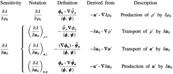
As in Marquet et al. (Reference Marquet, Sipp and Jacquin2008), we can follow through the derivations of the partial sensitivities and determine the origins of each of the additive terms. These origins reveal the physical mechanisms underlying the partial sensitivities. First, the partial sensitivity to base flow density modifications
 $\unicode[STIX]{x2202}\unicode[STIX]{x1D706}/\unicode[STIX]{x2202}\unicode[STIX]{x1D70C}_{0}$
(2.32) is ultimately derived from the
 $-\boldsymbol{u}^{\prime }\boldsymbol{\cdot }\unicode[STIX]{x1D735}\unicode[STIX]{x1D6FF}\unicode[STIX]{x1D70C}_{0}$
term in the density component of the operator perturbation
 $\unicode[STIX]{x1D6FF}\mathscr{L}$
(2.27). Thus, it represents the production of density perturbations by
 $\unicode[STIX]{x1D6FF}\unicode[STIX]{x1D70C}_{0}$
.
Next, we can see that in the partial sensitivity to base flow velocity modifications (2.39), the additive term
 $-\bar{\unicode[STIX]{x1D713}}_{\unicode[STIX]{x1D70C}}\unicode[STIX]{x1D735}\unicode[STIX]{x1D719}_{\unicode[STIX]{x1D70C}}/\left<\unicode[STIX]{x1D753},\unicode[STIX]{x1D74D}\right>$
is derived from
 $-\unicode[STIX]{x1D6FF}\boldsymbol{u}_{0}\boldsymbol{\cdot }\unicode[STIX]{x1D735}\unicode[STIX]{x1D70C}^{\prime }$
in the density component of
 $\unicode[STIX]{x1D6FF}\mathscr{L}$
(2.34). Thus, it represents the transport of density perturbations by
 $\unicode[STIX]{x1D6FF}\boldsymbol{u}_{0}$
, which we denote by
 $$\begin{eqnarray}\displaystyle \left(\frac{\unicode[STIX]{x2202}\unicode[STIX]{x1D706}}{\unicode[STIX]{x2202}\boldsymbol{u}_{0}}\right)_{\unicode[STIX]{x1D70C},\text{t}}:=-\frac{\bar{\unicode[STIX]{x1D713}}_{\unicode[STIX]{x1D70C}}\unicode[STIX]{x1D735}\unicode[STIX]{x1D719}_{\unicode[STIX]{x1D70C}}}{\left<\unicode[STIX]{x1D753},\unicode[STIX]{x1D74D}\right>}. & & \displaystyle\end{eqnarray}$$
By the same mechanism as Marquet et al. (Reference Marquet, Sipp and Jacquin2008), the terms
 $-(\unicode[STIX]{x1D735}\unicode[STIX]{x1D753}_{\boldsymbol{u}})\boldsymbol{\cdot }\bar{\unicode[STIX]{x1D74D}}_{\boldsymbol{u}}/\left<\unicode[STIX]{x1D753},\unicode[STIX]{x1D74D}\right>$
and
 $\unicode[STIX]{x1D753}_{\boldsymbol{u}}\boldsymbol{\cdot }\unicode[STIX]{x1D735}\bar{\unicode[STIX]{x1D74D}}_{\boldsymbol{u}}/\left<\unicode[STIX]{x1D753},\unicode[STIX]{x1D74D}\right>$
in (2.39) are respectively derived from
 $-\unicode[STIX]{x1D6FF}\boldsymbol{u}_{0}\boldsymbol{\cdot }\unicode[STIX]{x1D735}\boldsymbol{u}^{\prime }$
and
 $-\boldsymbol{u}^{\prime }\boldsymbol{\cdot }\unicode[STIX]{x1D735}\unicode[STIX]{x1D6FF}\boldsymbol{u}_{0}$
in (2.34). Therefore, they respectively represent the transport and production of velocity perturbations by
 $\unicode[STIX]{x1D6FF}\boldsymbol{u}_{0}$
, which we denote by
 $$\begin{eqnarray}\displaystyle & \displaystyle \left(\frac{\unicode[STIX]{x2202}\unicode[STIX]{x1D706}}{\unicode[STIX]{x2202}\boldsymbol{u}_{0}}\right)_{\boldsymbol{u},\text{t}}:=-\frac{(\unicode[STIX]{x1D735}\unicode[STIX]{x1D753}_{\boldsymbol{u}})\boldsymbol{\cdot }\bar{\unicode[STIX]{x1D74D}}_{\boldsymbol{u}}}{\left<\unicode[STIX]{x1D753},\unicode[STIX]{x1D74D}\right>}, & \displaystyle\end{eqnarray}$$
 $$\begin{eqnarray}\displaystyle & \displaystyle \left(\frac{\unicode[STIX]{x2202}\unicode[STIX]{x1D706}}{\unicode[STIX]{x2202}\boldsymbol{u}_{0}}\right)_{\boldsymbol{u},\text{p}}:=\frac{\unicode[STIX]{x1D753}_{\boldsymbol{u}}\boldsymbol{\cdot }\unicode[STIX]{x1D735}\bar{\unicode[STIX]{x1D74D}}_{\boldsymbol{u}}}{\left<\unicode[STIX]{x1D753},\unicode[STIX]{x1D74D}\right>}. & \displaystyle\end{eqnarray}$$
The additive terms in the partial sensitivities.

2.3 Remarks on total sensitivity
The partial sensitivity analysis in the prior section is most useful for understanding the effects of base flow density and velocity modifications, individually, on the flow stability. Conceptually, it is reasonable to imagine that the density and velocity modifications should be linked in practice. For instance, we may wish to determine to the change in the stability of a stratified bluff-body wake as the Froude number changes from
 $Fr$
to some
 $Fr+\unicode[STIX]{x1D6FF}Fr$
. In this case, both
 $\unicode[STIX]{x1D70C}_{0}$
and
 $\boldsymbol{u}_{0}$
would be expected to change.
If
 $\unicode[STIX]{x1D70C}_{0}$
and
 $\boldsymbol{u}_{0}$
change together, the shift in the linearised dynamics would be given by the sum of the right-hand sides of (2.27) and (2.34), that is,
 $$\begin{eqnarray}\displaystyle \unicode[STIX]{x1D6FF}\mathscr{L}\left[\begin{array}{@{}c@{}}\unicode[STIX]{x1D70C}^{\prime }\\ \boldsymbol{u}^{\prime }\end{array}\right]=\left[\begin{array}{@{}c@{}}-\unicode[STIX]{x1D6FF}\boldsymbol{u}_{0}\boldsymbol{\cdot }\unicode[STIX]{x1D735}\unicode[STIX]{x1D70C}^{\prime }-\boldsymbol{u}^{\prime }\boldsymbol{\cdot }\unicode[STIX]{x1D735}\unicode[STIX]{x1D6FF}\unicode[STIX]{x1D70C}_{0}\\ -\unicode[STIX]{x1D6FF}\boldsymbol{u}_{0}\boldsymbol{\cdot }\unicode[STIX]{x1D735}\boldsymbol{u}^{\prime }-\boldsymbol{u}^{\prime }\boldsymbol{\cdot }\unicode[STIX]{x1D735}\unicode[STIX]{x1D6FF}\boldsymbol{u}_{0}\end{array}\right]. & & \displaystyle\end{eqnarray}$$
It then follows that the eigenvalue perturbation is
 $$\begin{eqnarray}\displaystyle \unicode[STIX]{x1D6FF}\unicode[STIX]{x1D706}=\left<\frac{\unicode[STIX]{x2202}\unicode[STIX]{x1D706}}{\unicode[STIX]{x2202}\unicode[STIX]{x1D70C}_{0}},\unicode[STIX]{x1D6FF}\unicode[STIX]{x1D70C}_{0}\right>+\left<\frac{\unicode[STIX]{x2202}\unicode[STIX]{x1D706}}{\unicode[STIX]{x2202}\boldsymbol{u}_{0}},\unicode[STIX]{x1D6FF}\boldsymbol{u}_{0}\right>, & & \displaystyle\end{eqnarray}$$
which is in line with our interpretation of the partial sensitivities as partial derivatives.
If we are further able to express the base flow velocity modification
 $\unicode[STIX]{x1D6FF}\boldsymbol{u}_{0}$
in terms of the base flow density modification
 $\unicode[STIX]{x1D6FF}\unicode[STIX]{x1D70C}_{0}$
via the Jacobian equation
 $$\begin{eqnarray}\displaystyle \unicode[STIX]{x1D6FF}\boldsymbol{u}_{0}=\frac{\unicode[STIX]{x2202}\boldsymbol{u}_{0}}{\unicode[STIX]{x2202}\unicode[STIX]{x1D70C}_{0}}\unicode[STIX]{x1D6FF}\unicode[STIX]{x1D70C}_{0}, & & \displaystyle\end{eqnarray}$$
then (2.45) becomes
 $$\begin{eqnarray}\displaystyle \unicode[STIX]{x1D6FF}\unicode[STIX]{x1D706} & = & \displaystyle \displaystyle \left<\frac{\unicode[STIX]{x2202}\unicode[STIX]{x1D706}}{\unicode[STIX]{x2202}\unicode[STIX]{x1D70C}_{0}},\unicode[STIX]{x1D6FF}\unicode[STIX]{x1D70C}_{0}\right>+\left<\frac{\unicode[STIX]{x2202}\unicode[STIX]{x1D706}}{\unicode[STIX]{x2202}\boldsymbol{u}_{0}},\frac{\unicode[STIX]{x2202}\boldsymbol{u}_{0}}{\unicode[STIX]{x2202}\unicode[STIX]{x1D70C}_{0}}\unicode[STIX]{x1D6FF}\unicode[STIX]{x1D70C}_{0}\right>\end{eqnarray}$$
 $$\begin{eqnarray}\displaystyle & = & \displaystyle \displaystyle \left<\frac{\unicode[STIX]{x2202}\unicode[STIX]{x1D706}}{\unicode[STIX]{x2202}\unicode[STIX]{x1D70C}_{0}},\unicode[STIX]{x1D6FF}\unicode[STIX]{x1D70C}_{0}\right>+\int _{\unicode[STIX]{x1D6FA}}\frac{\unicode[STIX]{x2202}\unicode[STIX]{x1D706}}{\unicode[STIX]{x2202}\boldsymbol{u}_{0}}\boldsymbol{\cdot }\frac{\unicode[STIX]{x2202}\boldsymbol{u}_{0}}{\unicode[STIX]{x2202}\unicode[STIX]{x1D70C}_{0}}\unicode[STIX]{x1D6FF}\unicode[STIX]{x1D70C}_{0}\,\text{d}V\end{eqnarray}$$
 $$\begin{eqnarray}\displaystyle & = & \displaystyle \displaystyle \left<\frac{\unicode[STIX]{x2202}\unicode[STIX]{x1D706}}{\unicode[STIX]{x2202}\unicode[STIX]{x1D70C}_{0}},\unicode[STIX]{x1D6FF}\unicode[STIX]{x1D70C}_{0}\right>+\left<\frac{\unicode[STIX]{x2202}\unicode[STIX]{x1D706}}{\unicode[STIX]{x2202}\boldsymbol{u}_{0}}\boldsymbol{\cdot }\frac{\unicode[STIX]{x2202}\boldsymbol{u}_{0}}{\unicode[STIX]{x2202}\unicode[STIX]{x1D70C}_{0}},\unicode[STIX]{x1D6FF}\unicode[STIX]{x1D70C}_{0}\right>.\end{eqnarray}$$
 $$\begin{eqnarray}\displaystyle \frac{\text{d}\unicode[STIX]{x1D706}}{\text{d}\unicode[STIX]{x1D70C}_{0}}:=\frac{\unicode[STIX]{x2202}\unicode[STIX]{x1D706}}{\unicode[STIX]{x2202}\unicode[STIX]{x1D70C}_{0}}+\frac{\unicode[STIX]{x2202}\unicode[STIX]{x1D706}}{\unicode[STIX]{x2202}\boldsymbol{u}_{0}}\boldsymbol{\cdot }\frac{\unicode[STIX]{x2202}\boldsymbol{u}_{0}}{\unicode[STIX]{x2202}\unicode[STIX]{x1D70C}_{0}}, & & \displaystyle\end{eqnarray}$$
then the eigenvalue perturbation from both
 $\unicode[STIX]{x1D6FF}\unicode[STIX]{x1D70C}_{0}$
, as well as
 $\unicode[STIX]{x1D6FF}\boldsymbol{u}_{0}$
induced by
 $\unicode[STIX]{x1D6FF}\unicode[STIX]{x1D70C}_{0}$
, is expressed conveniently as
 $$\begin{eqnarray}\displaystyle \unicode[STIX]{x1D6FF}\unicode[STIX]{x1D706}=\left<\frac{\text{d}\unicode[STIX]{x1D706}}{\text{d}\unicode[STIX]{x1D70C}_{0}},\unicode[STIX]{x1D6FF}\unicode[STIX]{x1D70C}_{0}\right>. & & \displaystyle\end{eqnarray}$$
The difficulty in utilising the total sensitivity (2.48) is that the Jacobian
 $\unicode[STIX]{x2202}\boldsymbol{u}_{0}/\unicode[STIX]{x2202}\unicode[STIX]{x1D70C}_{0}$
is numerically very large and difficult to compute in its explicit form. In discretised space, its size would typically be the number of spatial dimensions times the square of the number of grid points or cells. Therefore, (2.48) is unlikely to be a tractable computation for two- or three-dimensional flows. For this reason, we will not pursue the total sensitivity in this manuscript besides to state it here, and we will base our analyses on the partial sensitivities instead. Should there exist an efficient computation of the total sensitivity, however, it would provide a valuable extension to the results presented in this manuscript.
3 Example: stably density-stratified flow around a bluff body
3.1 Base flow and global modes
For the remainder of the manuscript, we discuss the
 $Re=30$
flow around a thin plate at a
 $90^{\circ }$
angle of attack. The plate is one non-dimensional unit high and 0.05 units thick, and is centred in a
 $200\times 200$
finite volume domain. An exception is made for the unstratified flow, for which the plate is centred in a domain that is 200 units wide and 30 units high. The full details of the computational methods are given in appendix A. We choose
 $Re=30$
because it is close to the critical value of 35 at which a supercritical Hopf bifurcation occurs for
 $Fr=\infty$
, as will be evident later. A Prandtl number of
 $Pr=7.19$
is chosen to match values approximately expected in oceanographic flows. The exact value of
 $Pr$
is not expected to make a large difference in our results (de Stadler et al.
Reference de Stadler, Sarkar and Brucker2010).
The base flows at
 $Fr=1$
, 8, and
 $\infty$
are shown respectively in figures 1–3. The expected features can be seen in these figures. Most notably, lee waves can be seen in the stratified flows. Given a lengthy set of assumptions – that the stratified flow is two-dimensional, incompressible, steady and inviscid; that the upstream density and velocity are functions of only
 $y$
; that there is no flow reversal; and that the Froude number is constant in the flow – the displacement
 $\unicode[STIX]{x1D702}$
of streamlines in lee waves is given by
 $$\begin{eqnarray}\displaystyle \unicode[STIX]{x1D6FB}^{2}\unicode[STIX]{x1D702}+\frac{\unicode[STIX]{x1D702}}{Fr^{2}}=0 & & \displaystyle\end{eqnarray}$$
(Turner Reference Turner1973, chap. 3.1). This essentially establishes that the lee wavelength is
 $2\unicode[STIX]{x03C0}Fr$
.
The stratified flow at
 $Fr=8$
; see the caption of figure 1.

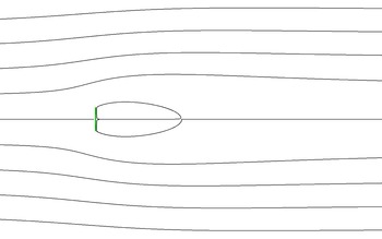
The unstratified flow from left to right around a vertical thin plate (green), at
 $Re=30$
.

At
 $Fr=1$
, the buoyancy effects are very strong, and notable lee waves of wavelength
 $2\unicode[STIX]{x03C0}$
are seen to emanate from the bluff body. Although the inertial effects of the flow are too large to support the complete blocking of the upstream flow by the bluff body (Yih Reference Yih1969), a significant upstream wake is nonetheless apparent. Furthermore, the recirculation region is shorter than in the
 $Fr=\infty$
case, since the fluid that is vertically deflected around the bluff body experiences a large restoring force back to the centre line. In the
 $Fr=8$
case, the lee waves have a larger wavelength of approximately
 $16\unicode[STIX]{x03C0}$
, and these waves are weaker in magnitude. In addition, the recirculation is longer than in the
 $Fr=1$
case because of the weaker buoyancy force. Finally, no density variations or lee waves are present when
 $Fr=\infty$
, as expected. Some additional discussion on the lee wavelength is given in § A.4.
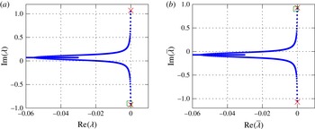
Next, we employ the Arnoldi iteration to compute the leading eigenvalues and eigenmodes; see the extended discussion in § A.1 for numerical details. It is very computationally expensive to resolve multiple eigenvalues and eigenmodes for these open flows, since spatial effects extend to great distances, and buoyancy waves pervade through the entire domain. Therefore, we only report on the most converged eigenvalue and eigenmode for each Froude number. Based on the distribution of Arnoldi eigenvalues at the conclusion of the iteration, it is likely that the modes we report are in fact the least stable ones. The mode at
 $Fr=\infty$
is in excellent agreement with the least stable mode for the circular cylinder (e.g. Marquet et al.
Reference Marquet, Sipp and Jacquin2008), and the mode at
 $Fr=1$
is consistent with the long-time behaviour of direct numerical simulations, as § 4.2 will show. As we will describe in more detail later, the mode we analyse for each Froude number is not a continuation of other modes we report at other Froude numbers. Therefore, we do not imply that the modes represent the same set of physics.
At
 $Fr=\infty$
, the Arnoldi iteration gives good convergence toward the least stable eigenvalue
 $\unicode[STIX]{x1D706}=-0.012\pm 0.642\text{i}$
and its complex conjugate. The corresponding direct and adjoint eigenmodes are shown in figure 4. As we discuss in greater detail in § A.2.1, the density components of these modes is
 $\unicode[STIX]{x1D719}_{\unicode[STIX]{x1D70C}}=\unicode[STIX]{x1D713}_{\unicode[STIX]{x1D70C}}=0$
, so the modes are identical to the constant-density modes, even allowing for non-zero density perturbations
 $\unicode[STIX]{x1D70C}^{\prime }$
in the linearised equations. The eigenmodes of unstratified flows around bluff bodies are well understood at this point and have been discussed in many works (e.g. Giannetti & Luchini Reference Giannetti and Luchini2007). Figure 4 depicts the common features. The direct eigenmode is localised in a long downstream region, with spatially oscillating structures. On the other hand, the adjoint eigenmode is large immediately downstream of the bluff body, but the remaining wake is actually upstream because of the reversed base flow advection in (2.16).
The (a) direct and (b) adjoint velocity eigenmodes of the
 $Fr=\infty$
flow, corresponding to the least stable eigenvalue
 $\unicode[STIX]{x1D706}=-0.012+0.642\text{i}$
; shown as the pointwise magnitude and streamlines of (a)
 $\text{Re}(\unicode[STIX]{x1D753}_{\boldsymbol{u}})$
and (b)
 $\text{Re}(\unicode[STIX]{x1D74D}_{\boldsymbol{u}})$
.

In contrast, the eigenmodes contain remarkably different features at
 $Fr=1$
. For this computation, the Arnoldi iteration resolves the eigenvalue
 $\unicode[STIX]{x1D706}=-0.001\pm 0.902\text{i}$
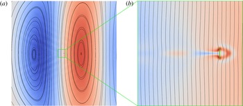
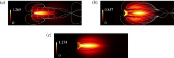
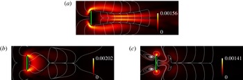
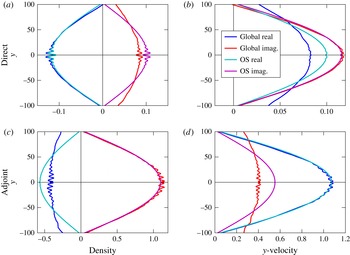
. The direct eigenmode is shown in figure 5, and the corresponding adjoint eigenmode is shown in figure 6. It is immediately apparent that large-scale structures (i.e. on the scale of the entire numerical mesh) are dominant in figures 5(a) and 6(a). These structures primarily consist of large vertical bands of density and vertical velocity; the density and vertical velocity are horizontally out of phase by a quarter period. The effects of the lee waves (figure 1) can also be seen in the direct eigenmodes. These large-scale structures are further analysed from a parallel flow perspective in § 4.1.
The direct eigenmode at
 $Fr=1$
corresponding to
 $\unicode[STIX]{x1D706}=-0.001-0.902\text{i}$
, shown as the real part of density (blue:
 $\text{Re}(\unicode[STIX]{x1D719}_{\unicode[STIX]{x1D70C}})<0$
; red:
 $\text{Re}(\unicode[STIX]{x1D719}_{\unicode[STIX]{x1D70C}})>0$
) and streamlines of
 $\text{Re}(\unicode[STIX]{x1D753}_{\boldsymbol{u}})$
. (a) The domain
 $[-60,60]\times [-60,60]$
; the right region rotates clockwise. (b) The domain
 $[-2,14]\times [-8,8]$
.

The adjoint eigenmode at
 $Fr=1$
corresponding to figure 5, shown as the real part of density (blue:
 $\text{Re}(\unicode[STIX]{x1D713}_{\unicode[STIX]{x1D70C}})<0$
; red:
 $\text{Re}(\unicode[STIX]{x1D713}_{\unicode[STIX]{x1D70C}})>0$
) and streamlines of
 $\text{Re}(\unicode[STIX]{x1D74D}_{\boldsymbol{u}})$
. (a) The domain
 $[-60,60]\times [-60,60]$
; the right region rotates clockwise. (b) The domain
 $[-7,2]\times [-4.5,4.5]$
.

A closer look at figures 5(b) and 6(b) reveals density and velocity structures associated with the downstream wake of the bluff body. These structures, however, are nowhere near as dominant as the downstream velocity structures for
 $Fr=\infty$
. In fact, the velocity streamlines of the direct and adjoint eigenmodes remain nearly vertical in the upstream and downstream wakes of the bluff body. In contrast, the eigenmode streamlines at
 $Fr=\infty$
(figure 4) form closed loops on the length scale of the bluff body.
Another important feature of the eigenmodes is the appearance of angled waves emanating from the bluff body. In the direct eigenmode (figure 5
a), an envelope downstream of the bluff body initially opens at an angle of
 $\unicode[STIX]{x1D703}=13^{\circ }$
from the horizontal direction. The angle increases to about
 $24^{\circ }$
at a distance of approximately
 $x=20$
downstream of the body. Wave crests can be seen inside this envelope. The envelope itself roughly demarcates the end of the lee waves in the base flow (figure 1). The adjoint eigenmode (figure 6
a) similarly contains an envelope – which is now upstream because of the reversed base flow direction in (2.16) – but the wave crests reside in the exterior of the envelope. This envelope initially opens at approximately
 $\unicode[STIX]{x1D703}=19^{\circ }$
before expanding to approximately
 $28^{\circ }$
further upstream.
It is well known that in an inviscid Boussinesq flow with a mass source or force oscillating at dimensional angular frequency
 $\tilde{\unicode[STIX]{x1D714}}$
in an open domain, gravity waves are emitted along beams at an angle of
 $\unicode[STIX]{x1D703}=\cos ^{-1}(\tilde{\unicode[STIX]{x1D714}}/{\tilde{N}})$
from the vertical (Voisin Reference Voisin1991; see also § A.4). This particular eigenmode has an angular frequency of
 $|\text{Im}(\unicode[STIX]{x1D706})|=0.901$
for a Brunt–Väisälä frequency of
 $N=1$
, with both quantities non-dimensionalised by convective time. Thus, the corresponding angle of wave transmission is predicted under this theory to be
 $\cos ^{-1}0.901=26^{\circ }$
. This angle is consistent with those observed in the direct and adjoint eigenmodes beyond the immediate wakes of the bluff body.
We remark that the use of a finite domain with artificial boundary conditions presents challenges in the determination of large-scale modal structures. In particular, the finite domain necessarily implies that any continua of eigenvalues and eigenmodes would be represented discretely instead. This may imply, for instance, that the horizontal wavelength is determined in part by the mesh size and the boundary conditions at the inlet and outlet. Nevertheless, the eigenmodes depicted in figures 5 and 6 still contain important near-wake features associated with the bluff body. We will see next that it is these wake features, and not the large-scale structures, that end up being important in the sensitivity calculations.
3.2 Sensitivity
3.2.1
 $Fr=\infty$
: unstratified flow

With the eigenmodes computed – noting that we have omitted the
 $Fr=8$
case for brevity – the partial sensitivities can now be computed. For
 $Fr=\infty$
, the partial sensitivity to base flow velocity modifications
 $\unicode[STIX]{x2202}\unicode[STIX]{x1D706}/\unicode[STIX]{x2202}\boldsymbol{u}_{0}$
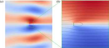
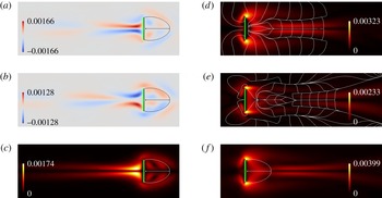
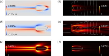
(2.39) is shown in figure 7. Since
 $\unicode[STIX]{x1D713}_{\unicode[STIX]{x1D70C}}=0$
, the partial sensitivity to base flow density modifications is
 $\unicode[STIX]{x2202}\unicode[STIX]{x1D706}/\unicode[STIX]{x2202}\unicode[STIX]{x1D70C}_{0}=0$
(see (2.32)). That is, the introduction of infinitesimal variations in the base flow density would have no first-order effects on the stability of this mode.
The partial sensitivities of the least stable eigenvalue
 $\unicode[STIX]{x1D706}=-0.012+0.642\text{i}$
of the
 $Fr=\infty$
flow, shown as pointwise vector magnitudes of (a)
 $\text{Re}(\unicode[STIX]{x2202}\unicode[STIX]{x1D706}/\unicode[STIX]{x2202}\boldsymbol{u}_{0})$
(streamlines enter the recirculation region), (b)
 $\text{Im}(\unicode[STIX]{x2202}\unicode[STIX]{x1D706}/\unicode[STIX]{x2202}\boldsymbol{u}_{0})$
(streamlines exit the recirculation region), and (c) the complex-valued
 $\unicode[STIX]{x2202}\unicode[STIX]{x1D706}/\unicode[STIX]{x2202}\boldsymbol{u}_{0}$
(with the recirculation bubble shown).

In addition,
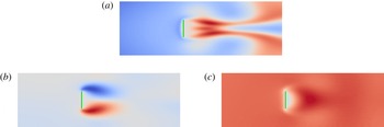
 $\unicode[STIX]{x2202}\unicode[STIX]{x1D706}/\unicode[STIX]{x2202}\boldsymbol{u}_{0}$
can be compared directly to the equivalent sensitivity presented in figure 7 of Marquet et al. (Reference Marquet, Sipp and Jacquin2008). Although our geometry is a transverse thin plate instead of a cylinder and our Reynolds number is below critical, the features of the sensitivity are essentially identical. The growth rate sensitivity (
 $\text{Re}(\unicode[STIX]{x2202}\unicode[STIX]{x1D706}/\unicode[STIX]{x2202}\boldsymbol{u}_{0})$
; figure 7
a) is largest in a horizontal band inside the recirculation region, and the primary destabilising base flow modification is the addition of upstream velocity in this region. The arrangement of the growth rate sensitivity streamlines indicates that this destabilising perturbation would increase the strength of the vorticity shed from the top and bottom surfaces of the plate.
On the other hand, the frequency sensitivity (
 $\text{Im}(\unicode[STIX]{x2202}\unicode[STIX]{x1D706}/\unicode[STIX]{x2202}\boldsymbol{u}_{0})$
; figure 7
b) is large not only in the recirculation region, but also in lobes above and below. At supercritical Reynolds numbers, this eigenmode corresponds to vortex shedding; therefore, the frequency sensitivity indicates that the addition of upstream velocity near the plate, and downstream velocity in the near wake, would accelerate the rate of vortex shedding. This is an intuitive result, since such a base flow velocity modification would increase both the rate of vorticity production at the plate tips, as well as the rate of vortex advection.
The partial sensitivity to base flow velocity modifications can be decomposed into components resulting from the transport and production of velocity perturbations by
 $\unicode[STIX]{x1D6FF}\boldsymbol{u}_{0}$
. Again, since
 $\unicode[STIX]{x1D719}_{\unicode[STIX]{x1D70C}}=\unicode[STIX]{x1D713}_{\unicode[STIX]{x1D70C}}=0$
, the transport and production of density perturbations are zero to first order (see table 1). The decomposition of the growth rate sensitivity
 $\text{Re}(\unicode[STIX]{x2202}\unicode[STIX]{x1D706}/\unicode[STIX]{x2202}\boldsymbol{u}_{0})$
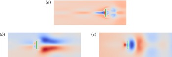
is shown in figure 8 and can be compared to figure 8 of Marquet et al. (Reference Marquet, Sipp and Jacquin2008). Once again, the features are largely identical. The transport component is concentrated more upstream than the production component, and is smaller in magnitude. Also, one set of
 $\text{Re}((\unicode[STIX]{x2202}\unicode[STIX]{x1D706}/\unicode[STIX]{x2202}\boldsymbol{u}_{0})_{\boldsymbol{u},\text{t}})$
streamlines roughly matches the recirculation streamlines.
The breakdown of
 $\text{Re}(\unicode[STIX]{x2202}\unicode[STIX]{x1D706}/\unicode[STIX]{x2202}\boldsymbol{u}_{0})$
(figure 7
a) into components at
 $Fr=\infty$
, each shown as pointwise vector magnitudes and streamlines. (a) The transport of velocity perturbations
 $\text{Re}((\unicode[STIX]{x2202}\unicode[STIX]{x1D706}/\unicode[STIX]{x2202}\boldsymbol{u}_{0})_{\boldsymbol{u},\text{t}})$
. (b) The production of velocity perturbations
 $\text{Re}((\unicode[STIX]{x2202}\unicode[STIX]{x1D706}/\unicode[STIX]{x2202}\boldsymbol{u}_{0})_{\boldsymbol{u},\text{p}})$
. The streamlines are directed into the recirculation bubble.

Some minor differences between this case and the critical cylinder flow can be seen. For instance, the transport component is comparatively larger and extends further downstream than in the cylinder flow. This may be the effect of the subcritical Reynolds number in our example, as opposed to the critical Reynolds number used by Marquet et al. (Reference Marquet, Sipp and Jacquin2008). In parallel and weakly non-parallel flow theory, a lower Reynolds number would generally cause the instability type to favour the convective (i.e. transport) type over the absolute (i.e. production) type (see, e.g. Bagheri et al. Reference Bagheri, Henningson, Hœpffner and Schmid2009). The differences between our example and that of Marquet et al., however, are minor compared to the difference between the behaviours at infinite and finite Froude numbers.
3.2.2
$Fr=1$
: strong stratification

For the eigenvalue
 $\unicode[STIX]{x1D706}=-0.001-0.902\text{i}$
in the
 $Fr=1$
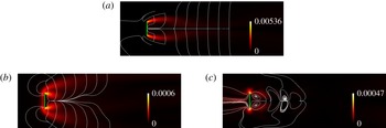
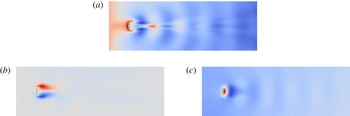
flow, the partial sensitivity to base flow velocity modifications is shown in figure 9(d–f). We immediately notice two ways in which the sensitivity to base flow velocity modifications differs from the
 $Fr=\infty$
case (figure 7). First, the sensitivity region is more concentrated near the top and bottom tips of the plate when
 $Fr=1$
. In particular, figure 9(d) shows that it is maximally destabilising to add a vertical component to the base flow there toward the plate centre. An intuitive explanation of this effect is that the addition of such a base flow perturbation would compress the recirculation bubble. Furthermore, the buoyancy forces are particularly large in those two regions, since the flow there has been deflected by a non-trivial vertical displacement. Therefore, a modification of the base flow velocity there would make a large impact in the characteristics of the flow. This modification is examined in § 4.2.
The partial sensitivities of the
 $Fr=1$
flow, for the least stable eigenvalue
 $\unicode[STIX]{x1D706}=-0.001-0.902\text{i}$
. The sensitivities are shown as (a)
 $\text{Re}(\unicode[STIX]{x2202}\unicode[STIX]{x1D706}/\unicode[STIX]{x2202}\unicode[STIX]{x1D70C}_{0})$
, (b)
 $\text{Im}(\unicode[STIX]{x2202}\unicode[STIX]{x1D706}/\unicode[STIX]{x2202}\unicode[STIX]{x1D70C}_{0})$
and (c)
 $|\unicode[STIX]{x2202}\unicode[STIX]{x1D706}/\unicode[STIX]{x2202}\unicode[STIX]{x1D70C}_{0}|$
. Also shown are pointwise vector magnitudes of (d)
 $\text{Re}(\unicode[STIX]{x2202}\unicode[STIX]{x1D706}/\unicode[STIX]{x2202}\boldsymbol{u}_{0})$
, (e)
 $\text{Im}(\unicode[STIX]{x2202}\unicode[STIX]{x1D706}/\unicode[STIX]{x2202}\boldsymbol{u}_{0})$
, and (f) the complex-valued
 $\unicode[STIX]{x2202}\unicode[STIX]{x1D706}/\unicode[STIX]{x2202}\boldsymbol{u}_{0}$
. Streamlines enter the recirculation region in (d,e). The recirculation region is shown in (a–c,f).

Second, the sensitivity is two to three orders of magnitude smaller. We note that the normalised denominator
 $\left<\unicode[STIX]{x1D753}/\Vert \unicode[STIX]{x1D753}\Vert ,\unicode[STIX]{x1D74D}/\Vert \unicode[STIX]{x1D74D}\Vert \right>$
of the partial sensitivities is 0.0229 for
 $Fr=\infty$
and 0.683 for
 $Fr=1$
. Seeing from (2.26) that
 $\left<\unicode[STIX]{x1D753},\unicode[STIX]{x1D74D}\right>^{-1}$
scales the eigenvalue perturbation
 $\unicode[STIX]{x1D6FF}\unicode[STIX]{x1D706}$
for a given linearised flow operator perturbation
 $\unicode[STIX]{x1D6FF}\mathscr{L}$
– and using
 $\Vert \unicode[STIX]{x1D753}\Vert$
and
 $\Vert \unicode[STIX]{x1D74D}\Vert$
to scale the eigenmodes – it is evident that the global overlap between
 $\unicode[STIX]{x1D753}$
and
 $\unicode[STIX]{x1D74D}$
causes
 $\unicode[STIX]{x1D706}$
to be less ‘mobile’ in the
 $Fr=1$
case than when
 $Fr=\infty$
. For an inviscid uniform base flow in the limit of an infinite control volume, the behaviour of
 $\left<\unicode[STIX]{x1D753},\unicode[STIX]{x1D74D}\right>$
is examined in § 4.1.2.
We briefly comment that this eigenvalue mobility can be related to the non-normality of the flow. The values of
 $\left<\unicode[STIX]{x1D753}/\Vert \unicode[STIX]{x1D753}\Vert ,\unicode[STIX]{x1D74D}/\Vert \unicode[STIX]{x1D74D}\Vert \right>$
indicate that the
 $Fr=\infty$
flow is more strongly non-normal than the
 $Fr=1$
flow. Thus, we can expect that the
 $\unicode[STIX]{x1D716}$
-pseudospectrum corresponding to
 $\unicode[STIX]{x1D706}$
(i.e. the values
 $\unicode[STIX]{x1D707}\in \mathbb{C}$
in the vicinity of
 $\unicode[STIX]{x1D706}$
such that
 $\Vert (\unicode[STIX]{x1D707}-\mathscr{L})^{-1}\Vert \geqslant \unicode[STIX]{x1D716}^{-1}$
) occupies a larger region of the complex plane. In essence,
 $\unicode[STIX]{x1D706}$
is easier to move, requiring a smaller base flow modification, when
 $Fr=\infty$
than when
 $Fr=1$
. Trefethen et al. (Reference Trefethen, Trefethen, Reddy and Driscoll1993) discuss the theory of non-normality in greater detail.
We also note that the vector directions of
 $\text{Re}(\unicode[STIX]{x2202}\unicode[STIX]{x1D706}/\unicode[STIX]{x2202}\boldsymbol{u}_{0})$
are approximately the same between
 $Fr=\infty$
(figure 7
a) and
 $Fr=1$
(figure 9
d). In both cases, the maximally destabilising base flow modification involves injecting additional base flow into the recirculation bubble. The vector directions corresponding to increasing or decreasing frequency are also the same. Although figure 7(b) and figure 9(e) have reversed vector directions of
 $\text{Im}(\unicode[STIX]{x2202}\unicode[STIX]{x1D706}/\unicode[STIX]{x2202}\boldsymbol{u}_{0})$
, the signs of
 $\text{Im}(\unicode[STIX]{x1D706})$
are also reversed. Therefore, at
 $Fr=1$
, an upstream injection of velocity just downstream of the body, as well as a downstream injection of velocity further downstream, would increase the frequency of the mode, as with
 $Fr=\infty$
.
The partial sensitivity to base flow density modifications (2.32) is shown in figure 9(a–c). We remind that this partial sensitivity is zero for the eigenmode we study at
 $Fr=\infty$
. At
 $Fr=1$
, the key feature of
 $\unicode[STIX]{x2202}\unicode[STIX]{x1D706}/\unicode[STIX]{x2202}\unicode[STIX]{x1D70C}_{0}$
is that it primarily lies upstream of the bluff body. This attribute is in stark contrast to constant-density sensitivity analyses (e.g. Giannetti & Luchini Reference Giannetti and Luchini2007; Marquet et al.
Reference Marquet, Sipp and Jacquin2008), which place the entirety of the sensitivity region downstream of bluff bodies. Whereas the velocity component of the sensitivity is driven primarily by the recirculation downstream of the body (e.g. as commented by Giannetti et al.
Reference Giannetti, Camarri and Luchini2010), the density component is most affected by the upstream wake visible in figure 1. In § 4.2, we will employ time-resolved simulations to explore the effect of both density and velocity modifications on the linearised dynamics at
 $Fr=1$
.
As summarised in table 1, the partial sensitivities can be decomposed into four different components. The partial sensitivity to base flow density modifications, as just described, arises from the production of density perturbations by
 $\unicode[STIX]{x1D6FF}\unicode[STIX]{x1D70C}_{0}$
. The partial sensitivity to base flow velocity modifications, however, can be decomposed into three components shown in figure 10. The transport of density perturbations by
 $\unicode[STIX]{x1D6FF}\boldsymbol{u}_{0}$
(figure 10
a) is unique to varying density flows. Like the density production mechanism, it acts in a region that extends upstream of the bluff body, though not to the extent seen in figure 9(a). It also extends significantly further downstream than the other three mechanisms. The upstream location of the two density-related components does not come as a complete surprise, since density-stratified flows exhibit upstream wakes (Yih Reference Yih1969).
The breakdown of
 $\text{Re}(\unicode[STIX]{x2202}\unicode[STIX]{x1D706}/\unicode[STIX]{x2202}\boldsymbol{u}_{0})$
(figure 9
d) into various components at
 $Fr=1$
, each shown as pointwise vector magnitudes and streamlines. (a) The transport of density perturbations
 $\text{Re}((\unicode[STIX]{x2202}\unicode[STIX]{x1D706}/\unicode[STIX]{x2202}\boldsymbol{u}_{0})_{\unicode[STIX]{x1D70C},\text{t}})$
. (b) The transport of velocity perturbations
 $\text{Re}((\unicode[STIX]{x2202}\unicode[STIX]{x1D706}/\unicode[STIX]{x2202}\boldsymbol{u}_{0})_{\boldsymbol{u},\text{t}})$
. (c) The production of velocity perturbations
 $\text{Re}((\unicode[STIX]{x2202}\unicode[STIX]{x1D706}/\unicode[STIX]{x2202}\boldsymbol{u}_{0})_{\boldsymbol{u},\text{p}})$
. Streamlines are directed away from the centre horizontal line in (a) and into the recirculation region in (b,c).

For
 $Fr=1$
, the transport and production of velocity perturbations by
 $\unicode[STIX]{x1D6FF}\boldsymbol{u}_{0}$
(figure 10
b,c) can be compared directly with their analogous components at
 $Fr=\infty$
(figure 8). Some notable differences are apparent. In the stratified flow, both mechanisms act much closer to the bluff body – and specifically, closer to the tips of the plate. Again, this feature can be attributed to the large buoyancy forces at the plate tips, as well as the shorter recirculation bubble caused by the buoyancy forces in the wake. In addition, the velocity transport is a somewhat more dominant mechanism than the production.
3.2.3
$Fr=8$
: mild stratification

Next, we discuss the partial sensitivities for the eigenvalue
 $\unicode[STIX]{x1D706}=-0.003+0.039\text{i}$
in the
 $Fr=8$
flow. The sensitivities are shown in figure 11. It is reasonable to hypothesise that the sensitivity regions for the
 $Fr=8$
flow would show an ‘in-between’ phase between the unstratified and the
 $Fr=1$
flows. To a limited extent, this conjecture is true. For instance, the partial sensitivity to base flow density modifications (figure 11
a–c) shows that a mix of upstream and downstream changes in the base flow density can influence the mode growth rate and frequency.
The partial sensitivities of the
 $Fr=8$
flow, for the eigenvalue
 $-0.003+0.039\text{i}$
. The sensitivities are shown as (a)
 $\text{Re}(\unicode[STIX]{x2202}\unicode[STIX]{x1D706}/\unicode[STIX]{x2202}\unicode[STIX]{x1D70C}_{0})$
, (b)
 $\text{Im}(\unicode[STIX]{x2202}\unicode[STIX]{x1D706}/\unicode[STIX]{x2202}\unicode[STIX]{x1D70C}_{0})$
and (c)
 $|\unicode[STIX]{x2202}\unicode[STIX]{x1D706}/\unicode[STIX]{x2202}\unicode[STIX]{x1D70C}_{0}|$
, as well as pointwise vector magnitudes of (d)
 $\text{Re}(\unicode[STIX]{x2202}\unicode[STIX]{x1D706}/\unicode[STIX]{x2202}\boldsymbol{u}_{0})$
, (e)
 $\text{Im}(\unicode[STIX]{x2202}\unicode[STIX]{x1D706}/\unicode[STIX]{x2202}\boldsymbol{u}_{0})$
, (f) the complex-valued
 $\unicode[STIX]{x2202}\unicode[STIX]{x1D706}/\unicode[STIX]{x2202}\boldsymbol{u}_{0}$
. In (d,e), streamlines are directed toward the centre horizontal line.

The partial sensitivity to base flow velocity modifications (figure 11
d–f) is largest nearly exactly on the boundary of the recirculation region. The sensitivity region is not as close to the bluff body as when
 $Fr=1$
. At the same time, it does not fill the recirculation region or extend as far downstream as when
 $Fr=\infty$
. The growth rate sensitivity (figure 11
d) is only non-trivial along thin bands on the boundary of the recirculation region. In contrast, for both the thin plate (figure 7
a) and the circular cylinder (Marquet et al.
Reference Marquet, Sipp and Jacquin2008), the unstratified growth rate exhibits the strongest sensitivity near the centreline of the recirculation bubble, with smaller lobes away from the centreline. The description of the frequency sensitivity is similar, except that compared to
 $Fr=1$
, the sensitivity region extends further from the bluff body in both the
 $Fr=8$
flow (figure 11
e) and the unstratified flow (figure 7
b), as well as in the unstratified circular cylinder flow (Marquet et al.
Reference Marquet, Sipp and Jacquin2008). A key difference is that in the
 $Fr=8$
flow, the frequency sensitivity is approximately one order of magnitude smaller than the growth rate sensitivity. We note that the eigenvalue in question has a small imaginary part compared to those examined for
 $Fr=1$
and
 $\infty$
.
The comparison among the
 $Fr=1$
, 8 and
 $\infty$
sensitivities, however, is an imperfect one. For instance, figures 9(a) and 11(a) show that base flow density modifications upstream of the bluff body have opposite growth rate effects between
 $Fr=1$
and 8. We stress that for our example, there is not a continuous morphing of
 $\unicode[STIX]{x2202}\unicode[STIX]{x1D706}/\unicode[STIX]{x2202}\boldsymbol{u}_{0}$
from
 $Fr=\infty$
to
 $Fr=1$
. In fact, neither a continuous morphing nor qualitatively identical sensitivities should be expected. The three sets of eigenvalues and eigenmodes analysed are not the same ones across Froude numbers, but are rather the most numerically converged ones at each
 $Fr$
(see § A.1). To observe the effect of the Froude number on a particular eigenvalue, eigenmode or sensitivity, computations would have to be run in much finer increments of
 $Fr$
, which we do not attempt here.
Figure 12 shows the breakdown of the growth rate sensitivity
 $\text{Re}(\unicode[STIX]{x2202}\unicode[STIX]{x1D706}/\unicode[STIX]{x2202}\boldsymbol{u}_{0})$
to base flow velocity modifications, again following table 1. It is apparent that the contribution
 $\text{Re}((\unicode[STIX]{x2202}\unicode[STIX]{x1D706}/\unicode[STIX]{x2202}\boldsymbol{u}_{0})_{\unicode[STIX]{x1D70C},\text{t}})$
from the transport of density perturbations by
 $\unicode[STIX]{x1D6FF}\boldsymbol{u}_{0}$
(figure 12
a) dominates this growth rate sensitivity. The growth rate sensitivity
 $\text{Re}(\unicode[STIX]{x2202}\unicode[STIX]{x1D706}/\unicode[STIX]{x2202}\unicode[STIX]{x1D70C}_{0})$
to base flow density modifications (figure 11
a) – corresponding to the production of density perturbations by
 $\unicode[STIX]{x1D6FF}\unicode[STIX]{x1D70C}_{0}$
– is also approximately an order of magnitude larger than the components from the transport and production of velocity perturbations by
 $\unicode[STIX]{x1D6FF}\boldsymbol{u}_{0}$
(figure 12
b,c). These features are in contrast to the breakdown for
 $Fr=1$
shown in figures 9(a) and 10, where all four components have similar magnitudes. Since the production and transport of density perturbations are features unique to density-varying flows, the growth rate sensitivities in this
 $Fr=8$
case are actually dominated by density effects.
The breakdown of
 $\text{Re}(\unicode[STIX]{x2202}\unicode[STIX]{x1D706}/\unicode[STIX]{x2202}\boldsymbol{u}_{0})$
(figure 11
d) into various components at
 $Fr=8$
, each shown as pointwise vector magnitudes and streamlines. (a) The transport of density perturbations
 $\text{Re}((\unicode[STIX]{x2202}\unicode[STIX]{x1D706}/\unicode[STIX]{x2202}\boldsymbol{u}_{0})_{\unicode[STIX]{x1D70C},\text{t}})$
. (b) The transport of velocity perturbations
 $\text{Re}((\unicode[STIX]{x2202}\unicode[STIX]{x1D706}/\unicode[STIX]{x2202}\boldsymbol{u}_{0})_{\boldsymbol{u},\text{t}})$
. (c) The production of velocity perturbations
 $\text{Re}((\unicode[STIX]{x2202}\unicode[STIX]{x1D706}/\unicode[STIX]{x2202}\boldsymbol{u}_{0})_{\boldsymbol{u},\text{p}})$
. All streamlines are directed into the recirculation region.

It is difficult to provide a rigorous explanation for this difference. As stated above, the eigenmode analysed for
 $Fr=8$
is not equivalent to the one shown for
 $Fr=1$
. Thus, the two modes exhibit different physics, and it is expected that their sensitivity characteristics would not be identical. We comment, however, that some qualitative similarities can also be found. For instance, the transport of velocity perturbations (figures 10
b and 12
b) is concentrated in lobes protruding from the bluff body into the recirculation region, whereas the production of velocity perturbations (figures 10
c and 12
c) is concentrated at the tips of the plate. The general nature of the sensitivity components cannot be described or derived simply, and merits further study.
4 Theory and numerical experiments on model systems
4.1 Predictions from parallel flow theory
In § 3.1, the direct and adjoint eigenmodes for the
 $Fr=1$
flow were depicted, and their features were described. It was then shown in § 3.2 that the eigenvalue sensitivity regions only occupied a small region local to the bluff body, as opposed to the large-scale structures found in the eigenmodes. In this section, we use inviscid and viscous parallel flow theory to explain some of these features. The main objectives in this section are to show that the global eigenmodes are consistent with predictions from canonical simplified representations, and to demonstrate in § 4.1.2 how the localised sensitivity structures arise from global eigenmode structures. Since we are now working exclusively with a stratified flow, we will use the alternate non-dimensionalisation of density (2.7), (2.8) that is more appropriate for stratified flows.
4.1.1 Inviscid uniform base flow
The large-scale structures found in the global eigenmodes (figures 5
a and 6
a) can be explained by employing canonical simplifications. In the most straightforward case, we make the assumption that the flow is inviscid, the bluff body is absent, and that the base flow is given by
 $\boldsymbol{u}_{0}=\boldsymbol{e}_{x}$
, the unit normal vector in the
 $x$
-direction. Defining the base flow density
 $\unicode[STIX]{x1D70C}_{\unicode[STIX]{x1D6E5}0}(\boldsymbol{x})=c-y$
for some
 $c$
and the density perturbation
 $\unicode[STIX]{x1D70C}_{\unicode[STIX]{x1D6E5}}^{\prime }(\boldsymbol{x},t):=\unicode[STIX]{x1D70C}_{\unicode[STIX]{x1D6E5}}(\boldsymbol{x},t)-\unicode[STIX]{x1D70C}_{\unicode[STIX]{x1D6E5}0}(\boldsymbol{x})$
, the linearised dynamics is given by
 $$\begin{eqnarray}\displaystyle & \displaystyle 0=\frac{\unicode[STIX]{x2202}u^{\prime }}{\unicode[STIX]{x2202}x^{\prime }}+\frac{\unicode[STIX]{x2202}v^{\prime }}{\unicode[STIX]{x2202}y^{\prime }}, & \displaystyle\end{eqnarray}$$
 $$\begin{eqnarray}\displaystyle & \displaystyle \frac{\unicode[STIX]{x2202}\unicode[STIX]{x1D70C}_{\unicode[STIX]{x1D6E5}}^{\prime }}{\unicode[STIX]{x2202}t}=-\frac{\unicode[STIX]{x2202}\unicode[STIX]{x1D70C}_{\unicode[STIX]{x1D6E5}}^{\prime }}{\unicode[STIX]{x2202}x}+v^{\prime }, & \displaystyle\end{eqnarray}$$
 $$\begin{eqnarray}\displaystyle & \displaystyle \frac{\unicode[STIX]{x2202}u^{\prime }}{\unicode[STIX]{x2202}t}=-\frac{\unicode[STIX]{x2202}u^{\prime }}{\unicode[STIX]{x2202}x}-\frac{\unicode[STIX]{x2202}p^{\prime }}{\unicode[STIX]{x2202}x}, & \displaystyle\end{eqnarray}$$
 $$\begin{eqnarray}\displaystyle & \displaystyle \frac{\unicode[STIX]{x2202}v^{\prime }}{\unicode[STIX]{x2202}t}=-\frac{\unicode[STIX]{x2202}v^{\prime }}{\unicode[STIX]{x2202}x}-\frac{\unicode[STIX]{x2202}p^{\prime }}{\unicode[STIX]{x2202}y}-\frac{\unicode[STIX]{x1D70C}_{\unicode[STIX]{x1D6E5}}^{\prime }}{Fr^{2}} & \displaystyle\end{eqnarray}$$
 $$\begin{eqnarray}\displaystyle \left(\left(\frac{\unicode[STIX]{x2202}}{\unicode[STIX]{x2202}t}+\frac{\unicode[STIX]{x2202}}{\unicode[STIX]{x2202}x}\right)^{2}\unicode[STIX]{x1D6FB}^{2}+\frac{1}{Fr^{2}}\frac{\unicode[STIX]{x2202}^{2}}{\unicode[STIX]{x2202}x^{2}}\right)\unicode[STIX]{x1D70C}_{\unicode[STIX]{x1D6E5}}^{\prime }=0. & & \displaystyle\end{eqnarray}$$
Similarly defining the adjoint density perturbation
 $\hat{\unicode[STIX]{x1D70C}}_{\unicode[STIX]{x1D6E5}}^{\prime }$
, the adjoint linearised dynamics is given by
 $$\begin{eqnarray}\displaystyle & \displaystyle 0=\frac{\unicode[STIX]{x2202}\hat{u} ^{\prime }}{\unicode[STIX]{x2202}x^{\prime }}+\frac{\unicode[STIX]{x2202}\hat{v}^{\prime }}{\unicode[STIX]{x2202}y^{\prime }}, & \displaystyle\end{eqnarray}$$
 $$\begin{eqnarray}\displaystyle & \displaystyle \frac{\unicode[STIX]{x2202}\hat{\unicode[STIX]{x1D70C}}_{\unicode[STIX]{x1D6E5}}^{\prime }}{\unicode[STIX]{x2202}t}=\frac{\unicode[STIX]{x2202}\hat{\unicode[STIX]{x1D70C}}_{\unicode[STIX]{x1D6E5}}^{\prime }}{\unicode[STIX]{x2202}x}-\frac{\hat{v}^{\prime }}{Fr^{2}}, & \displaystyle\end{eqnarray}$$
 $$\begin{eqnarray}\displaystyle & \displaystyle \frac{\unicode[STIX]{x2202}\hat{u} ^{\prime }}{\unicode[STIX]{x2202}t}=\frac{\unicode[STIX]{x2202}\hat{u} ^{\prime }}{\unicode[STIX]{x2202}x}-\frac{\unicode[STIX]{x2202}\hat{p}^{\prime }}{\unicode[STIX]{x2202}x}, & \displaystyle\end{eqnarray}$$
 $$\begin{eqnarray}\displaystyle & \displaystyle \frac{\unicode[STIX]{x2202}\hat{v}^{\prime }}{\unicode[STIX]{x2202}t}=\hat{\unicode[STIX]{x1D70C}}_{\unicode[STIX]{x1D6E5}}^{\prime }+\frac{\unicode[STIX]{x2202}\hat{v}^{\prime }}{\unicode[STIX]{x2202}x}-\frac{\unicode[STIX]{x2202}\hat{p}^{\prime }}{\unicode[STIX]{x2202}y} & \displaystyle\end{eqnarray}$$
 $$\begin{eqnarray}\displaystyle \left(\left(\frac{\unicode[STIX]{x2202}}{\unicode[STIX]{x2202}t}-\frac{\unicode[STIX]{x2202}}{\unicode[STIX]{x2202}x}\right)^{2}\unicode[STIX]{x1D6FB}^{2}+\frac{1}{Fr^{2}}\frac{\unicode[STIX]{x2202}^{2}}{\unicode[STIX]{x2202}x^{2}}\right)\hat{\unicode[STIX]{x1D70C}}_{\unicode[STIX]{x1D6E5}}^{\prime }=0. & & \displaystyle\end{eqnarray}$$
The leading eigenvalues (blue dots) of (a) the direct Orr–Sommerfeld equation (4.17) and (b) the adjoint equation (4.21), for the
 $Fr=1$
flow extracted from
 $x=-10$
. The eigenvalues predicted by the inviscid uniform base flow assumption (4.7) are shown as red
 $\times$
, and the global eigenvalue is shown as a green square.

If we now assume that the density perturbation has the form
 $$\begin{eqnarray}\displaystyle \unicode[STIX]{x1D70C}_{\unicode[STIX]{x1D6E5}}^{\prime }(x,y,t)=\text{e}^{\text{i}(k_{x}x+k_{y}y-\unicode[STIX]{x1D714}t)} & & \displaystyle\end{eqnarray}$$
for wavenumbers
 $k_{x},k_{y}\in \mathbb{R}$
and frequency
 $\unicode[STIX]{x1D714}\in \mathbb{C}$
, then we obtain the dispersion relation
 $$\begin{eqnarray}\displaystyle (k_{x}-\unicode[STIX]{x1D714})^{2}(k_{x}^{2}+k_{y}^{2})-\frac{k_{x}^{2}}{Fr^{2}}=0. & & \displaystyle\end{eqnarray}$$
An examination of the
 $Fr=1$
direct and adjoint eigenmode under investigation (figures 5
a and 6
a) reveals that this mode has a streamwise wavenumber of approximately
 $k_{x}=-0.071$
. Furthermore, we will assume
 $k_{y}=0$
because the real part of the mode is in phase with the imaginary part (not shown); thus, the vertical dependence is assumed to be an artefact of the finite domain and not a wave. The dispersion relation then yields
 $$\begin{eqnarray}\displaystyle \unicode[STIX]{x1D714}=k_{x}\pm Fr^{-1}, & & \displaystyle\end{eqnarray}$$
which evaluates to 0.929 or
 $-1.071$
, as shown in figure 13. Given the approximations made in this analysis, the frequency
 $\unicode[STIX]{x1D714}=k_{x}+Fr^{-1}=0.929$
is close to the complex value
 $\unicode[STIX]{x1D714}=\text{i}\unicode[STIX]{x1D706}=0.902-0.001\text{i}$
for the global eigenmode. The wave form of the density perturbation (4.5) also yields
 $$\begin{eqnarray}\displaystyle & \displaystyle u^{\prime }=-\frac{\text{i}k_{y}(k_{x}-\unicode[STIX]{x1D714})}{k_{x}}\unicode[STIX]{x1D70C}^{\prime }, & \displaystyle\end{eqnarray}$$
 $$\begin{eqnarray}\displaystyle & \displaystyle v^{\prime }=\text{i}(k_{x}-\unicode[STIX]{x1D714})\unicode[STIX]{x1D70C}^{\prime }, & \displaystyle\end{eqnarray}$$
 $u^{\prime }=0$
and
 $v^{\prime }=-\text{i}Fr^{-1}\unicode[STIX]{x1D70C}^{\prime }$
. The global eigenmode shown in figure 5(a) agrees closely with these relations.
Given (4.5), the adjoint perturbation must have the form
 $$\begin{eqnarray}\displaystyle \hat{\unicode[STIX]{x1D70C}}_{\unicode[STIX]{x1D6E5}}^{\prime }(x,y,t)=\text{e}^{\text{i}(k_{x}x+k_{y}y+\unicode[STIX]{x1D714}t)}. & & \displaystyle\end{eqnarray}$$
This adjoint perturbation yields the same dispersion relation as the direct perturbation (4.6), as well as
 $$\begin{eqnarray}\displaystyle & \displaystyle \hat{u} ^{\prime }=-\frac{\text{i}Fr^{2}k_{y}(k_{x}-\unicode[STIX]{x1D714})}{k_{x}}\hat{\unicode[STIX]{x1D70C}}_{\unicode[STIX]{x1D6E5}}^{\prime }, & \displaystyle\end{eqnarray}$$
 $$\begin{eqnarray}\displaystyle & \displaystyle \hat{v}^{\prime }=\text{i}Fr^{2}(k_{x}-\unicode[STIX]{x1D714})\hat{\unicode[STIX]{x1D70C}}_{\unicode[STIX]{x1D6E5}}^{\prime }. & \displaystyle\end{eqnarray}$$
4.1.2 Sensitivity in an inviscid uniform base flow
Given the inviscid uniform base flow analysis in § 4.1.1, we now discuss the disparity between the large-scale features found in the global eigenmodes (figures 5
a and 6
a) and the purely local structures in the sensitivity (e.g. figure 9). To perform this investigation, we compute the four transport and production mechanisms summarised in table 1 with the assumptions that
 $k_{y}=\unicode[STIX]{x2202}/\unicode[STIX]{x2202}y=0$
,
 $\unicode[STIX]{x1D719}_{\unicode[STIX]{x1D70C}}=\unicode[STIX]{x1D713}_{\unicode[STIX]{x1D70C}}=\text{e}^{\text{i}k_{x}x}$
and
 $\unicode[STIX]{x1D753}_{\boldsymbol{u}}=\left[\begin{array}{@{}cc@{}}\unicode[STIX]{x1D719}_{u} & \unicode[STIX]{x1D719}_{v}\end{array}\right]^{\text{T}}$
and
 $\unicode[STIX]{x1D74D}_{\boldsymbol{u}}=\left[\begin{array}{@{}cc@{}}\unicode[STIX]{x1D713}_{u} & \unicode[STIX]{x1D713}_{v}\end{array}\right]^{\text{T}}$
are given by (4.8) and (4.10). Note that we automatically have that
 $\unicode[STIX]{x1D719}_{u}=\unicode[STIX]{x1D713}_{u}=0$
. Thus, defining
 $V$
to be the volume of the domain, the denominator in the sensitivity terms evaluates to
 $$\begin{eqnarray}\displaystyle \left<\unicode[STIX]{x1D753},\unicode[STIX]{x1D74D}\right> & = & \displaystyle \displaystyle \int _{\unicode[STIX]{x1D6FA}}(\unicode[STIX]{x1D719}_{\unicode[STIX]{x1D70C}}\bar{\unicode[STIX]{x1D713}}_{\unicode[STIX]{x1D70C}}+\unicode[STIX]{x1D719}_{u}\bar{\unicode[STIX]{x1D713}}_{u}+\unicode[STIX]{x1D719}_{v}\bar{\unicode[STIX]{x1D713}}_{v})\,\text{d}V\end{eqnarray}$$
 $$\begin{eqnarray}\displaystyle & = & \displaystyle (1+Fr^{2}(k_{x}-\unicode[STIX]{x1D714})^{2})V\end{eqnarray}$$
 $$\begin{eqnarray}\displaystyle & = & \displaystyle 2V.\end{eqnarray}$$
First, the partial sensitivity to base flow density modifications, which describes the production of
 $\unicode[STIX]{x1D70C}^{\prime }$
by
 $\unicode[STIX]{x1D6FF}\unicode[STIX]{x1D70C}_{0}$
, is
 $$\begin{eqnarray}\displaystyle \frac{\unicode[STIX]{x2202}\unicode[STIX]{x1D706}}{\unicode[STIX]{x2202}\unicode[STIX]{x1D70C}_{0}} & = & \displaystyle \displaystyle \frac{1}{\left<\unicode[STIX]{x1D753},\unicode[STIX]{x1D74D}\right>}\left(\unicode[STIX]{x1D719}_{u}\frac{\unicode[STIX]{x2202}\bar{\unicode[STIX]{x1D713}}_{\unicode[STIX]{x1D70C}}}{\unicode[STIX]{x2202}x}+\unicode[STIX]{x1D719}_{v}\frac{\unicode[STIX]{x2202}\bar{\unicode[STIX]{x1D713}}_{\unicode[STIX]{x1D70C}}}{\unicode[STIX]{x2202}y}\right)\end{eqnarray}$$
 $$\begin{eqnarray}\displaystyle & = & \displaystyle 0.\end{eqnarray}$$
 $\unicode[STIX]{x1D70C}^{\prime }$
by
 $\unicode[STIX]{x1D6FF}\boldsymbol{u}_{0}$
is described by the term
 $$\begin{eqnarray}\displaystyle \displaystyle \left(\frac{\unicode[STIX]{x2202}\unicode[STIX]{x1D706}}{\unicode[STIX]{x2202}\boldsymbol{u}_{0}}\right)_{\unicode[STIX]{x1D70C},\text{t}} & = & \displaystyle \displaystyle -\frac{\bar{\unicode[STIX]{x1D713}}_{\unicode[STIX]{x1D70C}}}{\left<\unicode[STIX]{x1D753},\unicode[STIX]{x1D74D}\right>}\left[\begin{array}{@{}c@{}}\displaystyle \frac{\unicode[STIX]{x2202}\unicode[STIX]{x1D719}_{\unicode[STIX]{x1D70C}}}{\unicode[STIX]{x2202}x}\\ \displaystyle \frac{\unicode[STIX]{x2202}\unicode[STIX]{x1D719}_{\unicode[STIX]{x1D70C}}}{\unicode[STIX]{x2202}y}\end{array}\right]\end{eqnarray}$$
 $$\begin{eqnarray}\displaystyle & = & \displaystyle \displaystyle -\frac{\text{i}k_{x}}{2V}\boldsymbol{e}_{x};\end{eqnarray}$$
 $\boldsymbol{u}^{\prime }$
by
 $\unicode[STIX]{x1D6FF}\boldsymbol{u}_{0}$
is described by the term
 $$\begin{eqnarray}\displaystyle \displaystyle \left(\frac{\unicode[STIX]{x2202}\unicode[STIX]{x1D706}}{\unicode[STIX]{x2202}\boldsymbol{u}_{0}}\right)_{\boldsymbol{u},\text{t}} & = & \displaystyle \displaystyle -\frac{1}{\left<\unicode[STIX]{x1D753},\unicode[STIX]{x1D74D}\right>}\left[\begin{array}{@{}c@{}}\displaystyle \frac{\unicode[STIX]{x2202}\unicode[STIX]{x1D719}_{u}}{\unicode[STIX]{x2202}x}\bar{\unicode[STIX]{x1D713}}_{u}+\frac{\unicode[STIX]{x2202}\unicode[STIX]{x1D719}_{v}}{\unicode[STIX]{x2202}x}\bar{\unicode[STIX]{x1D713}}_{v}\\ \displaystyle \frac{\unicode[STIX]{x2202}\unicode[STIX]{x1D719}_{u}}{\unicode[STIX]{x2202}y}\bar{\unicode[STIX]{x1D713}}_{u}+\frac{\unicode[STIX]{x2202}\unicode[STIX]{x1D719}_{v}}{\unicode[STIX]{x2202}y}\bar{\unicode[STIX]{x1D713}}_{v}\end{array}\right]\end{eqnarray}$$
 $$\begin{eqnarray}\displaystyle & = & \displaystyle \frac{\text{i}Fr^{2}k_{x}(k_{x}-\unicode[STIX]{x1D714})^{2}}{2V}\boldsymbol{e}_{x};\end{eqnarray}$$
 $\boldsymbol{u}^{\prime }$
by
 $\unicode[STIX]{x1D6FF}\boldsymbol{u}_{0}$
is described by the term
 $$\begin{eqnarray}\displaystyle \displaystyle \left(\frac{\unicode[STIX]{x2202}\unicode[STIX]{x1D706}}{\unicode[STIX]{x2202}\boldsymbol{u}_{0}}\right)_{\boldsymbol{u},\text{p}} & = & \displaystyle \displaystyle \frac{1}{\left<\unicode[STIX]{x1D753},\unicode[STIX]{x1D74D}\right>}\left[\begin{array}{@{}c@{}}\displaystyle \unicode[STIX]{x1D719}_{u}\frac{\unicode[STIX]{x2202}\bar{\unicode[STIX]{x1D713}}_{u}}{\unicode[STIX]{x2202}x}+\unicode[STIX]{x1D719}_{v}\frac{\unicode[STIX]{x2202}\bar{\unicode[STIX]{x1D713}}_{u}}{\unicode[STIX]{x2202}y}\\ \displaystyle \unicode[STIX]{x1D719}_{u}\frac{\unicode[STIX]{x2202}\bar{\unicode[STIX]{x1D713}}_{v}}{\unicode[STIX]{x2202}x}+\unicode[STIX]{x1D719}_{v}\frac{\unicode[STIX]{x2202}\bar{\unicode[STIX]{x1D713}}_{v}}{\unicode[STIX]{x2202}y}\end{array}\right]\end{eqnarray}$$
 $$\begin{eqnarray}\displaystyle & = & \displaystyle \mathbf{0}.\end{eqnarray}$$
Therefore, we conclude that the partial sensitivity to base flow density modifications is always zero for the inviscid uniform base flow, and the partial sensitivity to base flow velocity modifications approaches zero in the limit of an unbounded domain (i.e.
 $V\rightarrow \infty$
). The non-zero sensitivities we actually observe (figures 9 and 11) must arise from differences between the global eigenmodes and the simple form
 $\unicode[STIX]{x1D719}_{\unicode[STIX]{x1D70C}}=\unicode[STIX]{x1D713}_{\unicode[STIX]{x1D70C}}=\text{e}^{\text{i}k_{x}x}$
. Since these differences are primarily caused by the bluff body (assuming that viscosity and diffusion are largely negligible away from the body), the sensitivities are largest in a local region near the thin plate. Hence, the localised sensitivity regions are able to arise from the global eigenmodes covering the entire domain.
4.1.3 Orr–Sommerfeld analysis
The parallel flow analysis so far can be made more accurate by relaxing the assumptions that the fluid is inviscid and that the base flow is uniform. By now assuming that the base flow is merely parallel, we arrive at an Orr–Sommerfeld-type analysis. The Orr–Sommerfeld equation, which is reviewed by Schmid & Henningson (Reference Schmid and Henningson2001) and White (Reference White2005) for constant-density flows, can be expressed as an analogous sixth-order ordinary differential equation for stratified flows (Koppel Reference Koppel1964; Maslowe & Thompson Reference Maslowe and Thompson1971). For our analysis, we choose to keep density and the
 $y$
-component of velocity separate, so our equation is a set of ordinary differential equations that is second order in density and fourth order in velocity.
The assumptions of this analysis are that the dynamics is governed by the linearised Boussinesq equations (2.13); that the base flow is given by
 $\unicode[STIX]{x1D70C}_{0}(y)$
and
 $\boldsymbol{u}_{0}(y)=\left[\begin{array}{@{}cc@{}}u_{0}(y) & 0\end{array}\right]^{\text{T}}$
; and that for a streamwise wavenumber
 $k$
, eigenvalue
 $\unicode[STIX]{x1D706}$
and amplitude functions
 $\unicode[STIX]{x1D70C}_{a}(y)$
and
 $\boldsymbol{u}_{a}(y)=\left[\begin{array}{@{}cc@{}}u_{a}(y) & v_{a}(y)\end{array}\right]^{\text{T}}$
, the infinitesimal flow perturbation from the base flow is
 $$\begin{eqnarray}\displaystyle \left[\begin{array}{@{}c@{}}\unicode[STIX]{x1D70C}_{\unicode[STIX]{x1D6E5}}^{\prime }(\boldsymbol{x},t)\\ \boldsymbol{u}^{\prime }(\boldsymbol{x},t)\end{array}\right]=\left[\begin{array}{@{}c@{}}\unicode[STIX]{x1D70C}_{a}(y)\\ \boldsymbol{u}_{a}(y)\end{array}\right]\text{e}^{\text{i}kx+\unicode[STIX]{x1D706}t}. & & \displaystyle\end{eqnarray}$$
With these assumptions, the generalised eigendecomposition of the resulting linearised dynamics is
 $$\begin{eqnarray}\displaystyle \left[\begin{array}{@{}cc@{}}\mathscr{L}_{\unicode[STIX]{x1D70C}} & \displaystyle -\frac{\text{d}\unicode[STIX]{x1D70C}_{0}}{\text{d}y}\\ k^{2}Fr^{-2} & \mathscr{L}_{v}\end{array}\right]\left[\begin{array}{@{}c@{}}\unicode[STIX]{x1D70C}_{a}\\ v_{a}\end{array}\right]=\unicode[STIX]{x1D706}\left[\begin{array}{@{}cc@{}}1 & 0\\ 0 & \displaystyle \frac{\text{d}^{2}}{\text{d}y^{2}}-k^{2}\end{array}\right]\left[\begin{array}{@{}c@{}}\unicode[STIX]{x1D70C}_{a}\\ v_{a}\end{array}\right], & & \displaystyle\end{eqnarray}$$
where
 $$\begin{eqnarray}\displaystyle & \displaystyle \mathscr{L}_{\unicode[STIX]{x1D70C}}:=-\text{i}ku_{0}+\frac{1}{Re\,Pr}\left(\frac{\text{d}^{2}}{\text{d}y^{2}}-k^{2}\right), & \displaystyle\end{eqnarray}$$
 $$\begin{eqnarray}\displaystyle & \displaystyle \mathscr{L}_{v}:=\text{i}k\left(\frac{\text{d}^{2}u_{0}}{\text{d}y^{2}}-u_{0}\left(\frac{\text{d}^{2}}{\text{d}y^{2}}-k^{2}\right)\right)+\frac{1}{Re}\left(\frac{\text{d}^{2}}{\text{d}y^{2}}-k^{2}\right)^{2}. & \displaystyle\end{eqnarray}$$
 $\unicode[STIX]{x1D70C}^{\prime }$
and
 $\boldsymbol{u}^{\prime }$
(table 2 in § A.3) are equivalent to
 $$\begin{eqnarray}\displaystyle \frac{\text{d}\unicode[STIX]{x1D70C}_{a}}{\text{d}y}=\frac{\text{d}v_{a}}{\text{d}y}=\frac{\text{d}^{2}v_{a}}{\text{d}y^{2}}=0 & & \displaystyle\end{eqnarray}$$
at the endpoints of
 $y$
.
Likewise, given
 $\hat{\boldsymbol{u}}_{a}(y)=\left[\begin{array}{@{}cc@{}}\hat{u} _{a}(y) & \hat{v}_{a}(y)\end{array}\right]^{\text{T}}$
and the form
 $$\begin{eqnarray}\displaystyle \left[\begin{array}{@{}c@{}}\hat{\unicode[STIX]{x1D70C}}^{\prime }(\boldsymbol{x},t)\\ \hat{\boldsymbol{u}}^{\prime }(\boldsymbol{x},t)\end{array}\right]=\left[\begin{array}{@{}c@{}}\hat{\unicode[STIX]{x1D70C}}_{a}(y)\\ \hat{\boldsymbol{u}}_{a}(y)\end{array}\right]\text{e}^{\text{i}kx+\bar{\unicode[STIX]{x1D706}}t}, & & \displaystyle\end{eqnarray}$$
the Orr–Sommerfeld-type generalised eigendecomposition for the adjoint linear Boussinesq equations (2.16) is
 $$\begin{eqnarray}\displaystyle \left[\begin{array}{@{}cc@{}}\mathscr{L}_{\unicode[STIX]{x1D70C}}^{\ast } & -Fr^{-2}\\ k^{2}\displaystyle \frac{\text{d}\unicode[STIX]{x1D70C}_{0}}{\text{d}y} & \mathscr{L}_{v}^{\ast }\end{array}\right]\left[\begin{array}{@{}c@{}}\hat{\unicode[STIX]{x1D70C}}_{a}\\ \hat{v}_{a}\end{array}\right]=\bar{\unicode[STIX]{x1D706}}\left[\begin{array}{@{}cc@{}}1 & 0\\ 0 & \displaystyle \frac{\text{d}^{2}}{\text{d}y^{2}}-k^{2}\end{array}\right]\left[\begin{array}{@{}c@{}}\hat{\unicode[STIX]{x1D70C}}_{a}\\ \hat{v}_{a}\end{array}\right], & & \displaystyle\end{eqnarray}$$
where
 $$\begin{eqnarray}\displaystyle & \displaystyle \mathscr{L}_{\unicode[STIX]{x1D70C}}^{\ast }:=\text{i}ku_{0}+\frac{1}{Re\,Pr}\left(\frac{\text{d}^{2}}{\text{d}y^{2}}-k^{2}\right), & \displaystyle\end{eqnarray}$$
 $$\begin{eqnarray}\displaystyle & \displaystyle \mathscr{L}_{v}^{\ast }:=\text{i}k\left(2\frac{\text{d}u_{0}}{\text{d}y}\frac{\text{d}}{\text{d}y}+u_{0}\left(\frac{\text{d}^{2}}{\text{d}y^{2}}-k^{2}\right)\right)+\frac{1}{Re}\left(\frac{\text{d}^{2}}{\text{d}y^{2}}-k^{2}\right)^{2}. & \displaystyle\end{eqnarray}$$
 $\hat{\unicode[STIX]{x1D70C}}^{\prime }$
and
 $\hat{\boldsymbol{u}}^{\prime }$
(table 2) are equivalent to
 $$\begin{eqnarray}\displaystyle \frac{\text{d}\hat{\unicode[STIX]{x1D70C}}_{a}}{\text{d}y}=\frac{\text{d}\hat{v}_{a}}{\text{d}y}=\frac{\text{d}^{2}\hat{v}_{a}}{\text{d}y^{2}}=0 & & \displaystyle\end{eqnarray}$$
at the endpoints of
 $y$
. The derivation of these equations is given in appendix B. We remark that since (4.21) is derived from the adjoint linearised Boussinesq equations for the inner product over the full domain (2.14), it is also the adjoint of (4.17) for the inner product over
 $y$
that corresponds to (2.14).
To compute these eigendecompositions, we first extract the base flow along the line
 $x=-10$
, and assume that the flow is everywhere parallel with
 $\unicode[STIX]{x1D70C}_{0}$
and
 $\boldsymbol{u}_{0}$
given by this profile. This base flow contains the transverse oscillations associated with the blocking and lee waves, as visible in figure 1(a). As before, we estimate
 $k=-0.071$
. Since we wish to simulate an infinite domain, we compute pseudospectral differentiation matrices using Hermite polynomials based on algorithms described by Weideman & Reddy (Reference Weideman and Reddy2000). Employing 247 Hermite quadrature points, the differentiation matrices allow us to represent (4.17) and (4.21) as generalised eigenvalue problems of size
 $494\times 494$
.
The Orr–Sommerfeld eigenmode corresponding to (a,b) the direct equation (4.17) and
 $\unicode[STIX]{x1D706}=-0.000-0.907\text{i}$
, and (c,d) the adjoint equation (4.21) and
 $\bar{\unicode[STIX]{x1D706}}=-0.000+0.907\text{i}$
: (a,c) depict the density component and (b,d) depict the
 $y$
-velocity component. Also shown are the profiles of the global modes (a,b)
 $\unicode[STIX]{x1D753}$
and (c,d)
 $\unicode[STIX]{x1D74D}$
along the line
 $x=-10$
.

The leading eigenvalues of (4.17) and (4.21) are shown in figure 13. The spectrum of the direct equation (4.17) contains the eigenvalue
 $\unicode[STIX]{x1D706}=-0.000-0.907\text{i}$
. As expected, the spectrum of the adjoint equation (4.21) contains the conjugate eigenvalue
 $\bar{\unicode[STIX]{x1D706}}=-0.000+0.907\text{i}$
. Both of these eigenvalues are close to the value
 $\unicode[STIX]{x1D706}=-0.001-0.902\text{i}$
computed from the global flow field.
Also, figure 14 shows the eigenmodes corresponding to these eigenvalues, and compares them with the profile of the global modes taken at
 $x=-10$
. The global modes are first normalised in the two-dimensional domain using the inner product in (2.14), and the slice at
 $x=-10$
is taken; the Orr–Sommerfeld modes are then scaled to match the global modes. Overall, we observe that the Orr–Sommerfeld analysis is able to capture the nature of the global direct eigenmodes, including the upstream waves associated with the blocking by the bluff body.
The differences between the Orr–Sommerfeld eigenmodes and the global eigenmodes are primarily a result of the different boundary conditions. The Hermite pseudospectral method assumes that quantities converge to 0 at
 $y\rightarrow \pm \infty$
, whereas we have only employed homogeneous Neumann conditions in the global eigenmodes. In addition, the agreement in the adjoint modes is not as good, because the relatively uniform base flow is insufficient for predicting the upstream-travelling oblique waves caused by the bluff body (figure 6
a). Nevertheless, this test validates the large-scale global mode structures shown in figures 5 and 6, as well as their corresponding eigenvalues. In addition, we can further conclude that the sensitivities shown in § 3 must be the result of local features not found in this parallel flow analysis.
4.2 Linearised simulations with modified base flow density
With the partial sensitivity theory developed in § 2.2, it is then natural to inquire what effects certain base flow modifications
 $\unicode[STIX]{x1D6FF}\unicode[STIX]{x1D70C}_{0}$
and
 $\unicode[STIX]{x1D6FF}\boldsymbol{u}_{0}$
would have on the linearised dynamics (2.13). Namely, if a certain
 $\unicode[STIX]{x1D6FF}\unicode[STIX]{x1D70C}_{0}$
or
 $\unicode[STIX]{x1D6FF}\boldsymbol{u}_{0}$
is expected to destabilise the flow by giving
 $\text{Re}(\unicode[STIX]{x1D6FF}\unicode[STIX]{x1D706})>0$
via (2.33) or (2.41), we would like to see what the resulting instability is. To that end, we perform time-resolved numerical experiments using the linearised Boussinesq equations (2.13) with
 $Fr=1$
. The simulations start with initial conditions
 $\unicode[STIX]{x1D70C}^{\prime }(\boldsymbol{x},0)$
and
 $\boldsymbol{u}^{\prime }(\boldsymbol{x},0)$
randomised from a uniform distribution at every grid point. Although such a velocity perturbation field will have non-zero divergence, the incompressible flow solver will ensure that
 $\boldsymbol{u}^{\prime }(\boldsymbol{x},t)$
at all subsequent time steps will be divergence free.
The density and velocity perturbation fields at
 $t=835.65$
is shown in figure 15. It is evident, for instance, that figure 15(a) contains the same downstream density wake structure as the eigenmode shown in figure 5(b). On the other hand, figure 15(c) shows that
 $\boldsymbol{u}^{\prime }$
consists primarily of vertical motions, as the eigenmode also exhibits in figure 5(b). Some velocity distortions are also apparent immediately downstream of the plate. Whereas figure 15(c) shows that the mode streamlines are primarily oriented upwards, figure 15(b) shows that downstream of the plate, the streamlines deflect to the right near the bottom, and to the left near the top. This, again, is in agreement with the global eigenmode in figure 5(b). Such a resemblance between the time-resolved flow and the eigenmode does not come as a surprise, since this eigenmode is one of the least stable ones present for this base flow.
A snapshot of a time-resolved linearised Boussinesq simulation using a random initial condition. Shown as (a)
 $\unicode[STIX]{x1D70C}^{\prime }$
, (b)
 $u^{\prime }$
and (c)
 $v^{\prime }$
. Red and blue respectively indicate positive and negative values.

To investigate the partial sensitivity to base flow density modifications, we next run a simulation with the base flow density perturbed to
 $\unicode[STIX]{x1D70C}_{0}+\unicode[STIX]{x1D6FF}\unicode[STIX]{x1D70C}_{0}$
, where
 $\unicode[STIX]{x1D6FF}\unicode[STIX]{x1D70C}_{0}=500\text{Re}(\text{d}\unicode[STIX]{x1D706}/\text{d}\unicode[STIX]{x1D70C}_{0})$
. Although the multiplicative coefficient may look large, we remind that
 $\text{Re}(\text{d}\unicode[STIX]{x1D706}/\text{d}\unicode[STIX]{x1D70C}_{0})$
is very small to begin with; see figure 9. The size of
 $\unicode[STIX]{x1D6FF}\unicode[STIX]{x1D70C}_{0}$
may be prohibitively large to prevent an accurate analysis as an infinitesimal base flow modification, but we choose this size for the ease of visual comparison to the unmodified base flow. For this experiment, the base flow velocity
 $\boldsymbol{u}_{0}$
and the initial conditions
 $\unicode[STIX]{x1D70C}^{\prime }(\boldsymbol{x},0)$
and
 $\boldsymbol{u}^{\prime }(\boldsymbol{x},0)$
remain unchanged.
Following the inner product equation relating
 $\unicode[STIX]{x1D6FF}\unicode[STIX]{x1D70C}_{0}$
and
 $\unicode[STIX]{x1D6FF}\unicode[STIX]{x1D706}$
(2.33), we would expect this base flow density perturbation to destabilise the flow. A snapshot of the linearised flow at a large
 $t$
is shown in figure 16. To highlight the slight destabilisation provided by this base flow modification, we emphasise that
 $\unicode[STIX]{x1D70C}^{\prime }$
is approximately an order of magnitude larger in figure 16(a) than in figure 15(a). The primary effect of this
 $\unicode[STIX]{x1D6FF}\unicode[STIX]{x1D70C}_{0}$
in
 $\unicode[STIX]{x1D70C}^{\prime }$
is to create a slightly unstable upstream oscillation along the centreline. This density wave prominently forms a few units upstream of the bluff body, propagates toward the body, and is horizontally compressed and vertically stretched as it meets the body. Part of the wave then climbs around the body and extends into the recirculation region.
A snapshot of a time-resolved linearised Boussinesq simulation using a random initial condition and a modified base flow density
 $\unicode[STIX]{x1D70C}_{0}+\unicode[STIX]{x1D6FF}\unicode[STIX]{x1D70C}_{0}$
, where
 $\unicode[STIX]{x1D6FF}\unicode[STIX]{x1D70C}_{0}=500\text{Re}(\text{d}\unicode[STIX]{x1D706}/\text{d}\unicode[STIX]{x1D70C}_{0})$
. Shown as (a)
 $\unicode[STIX]{x1D70C}^{\prime }$
(with colours slightly exaggerated for clarity), (b)
 $u^{\prime }$
and (c)
 $v^{\prime }$
. Red and blue respectively indicate positive and negative values.

An effect of
 $\unicode[STIX]{x1D6FF}\unicode[STIX]{x1D70C}_{0}$
can also be seen in
 $\boldsymbol{u}^{\prime }$
(figure 16
b,c). In particular, figure 16(c) shows the presence of a horizontal wave in
 $v^{\prime }$
that is not present in the absence of
 $\unicode[STIX]{x1D6FF}\unicode[STIX]{x1D70C}_{0}$
(figure 15
c). This velocity wave begins just upstream of the body and extends a few units downstream, and also propagates in the positive
 $x$
direction. Since the linearised velocity equation has not changed, the change in the behaviour of
 $v^{\prime }$
must be understood as an effect of
 $\unicode[STIX]{x1D70C}^{\prime }$
. Specifically, the linearised dynamics (2.13) reveals that if
 $\unicode[STIX]{x1D735}\unicode[STIX]{x1D6FF}\unicode[STIX]{x1D70C}_{0}$
points in the positive
 $y$
direction – e.g. upstream of the plate as in figure 9(a) – then a region with
 $v^{\prime }<0$
would see an increase in
 $\text{d}\unicode[STIX]{x1D70C}^{\prime }/\text{d}t$
via the density equation. The density perturbation
 $\unicode[STIX]{x1D70C}^{\prime }$
is then coupled back to
 $v^{\prime }$
via the momentum equation, such that an increase in
 $\unicode[STIX]{x1D70C}^{\prime }$
would cause a decrease in
 $\text{d}v^{\prime }/\text{d}t$
though the gravity term.
A snapshot of a time-resolved linearised Boussinesq simulation using a random initial condition and a modified base flow velocity
 $\boldsymbol{u}_{0}+\unicode[STIX]{x1D6FF}\boldsymbol{u}_{0}$
, where
 $\unicode[STIX]{x1D6FF}\boldsymbol{u}_{0}=350\text{Re}(\text{d}\unicode[STIX]{x1D706}/\text{d}\boldsymbol{u}_{0})$
. Shown as (a)
 $\unicode[STIX]{x1D70C}^{\prime }$
, (b)
 $u^{\prime }$
, and (c)
 $v^{\prime }$
. Red and blue respectively indicate positive and negative values.

Figure 17 is a snapshot of the linearised simulation with the unperturbed base flow density
 $\unicode[STIX]{x1D70C}_{0}$
, but with a modified base flow velocity
 $\boldsymbol{u}_{0}+\unicode[STIX]{x1D6FF}\boldsymbol{u}_{0}$
, where
 $\unicode[STIX]{x1D6FF}\boldsymbol{u}_{0}=350\text{Re}(\text{d}\unicode[STIX]{x1D706}/\text{d}\boldsymbol{u}_{0})$
. Once again, the initial conditions
 $\unicode[STIX]{x1D70C}^{\prime }(\boldsymbol{x},0)$
and
 $\boldsymbol{u}^{\prime }(\boldsymbol{x},0)$
are unchanged. Since the growth rate sensitivity
 $\text{Re}(\text{d}\unicode[STIX]{x1D706}/\text{d}\boldsymbol{u}_{0})$
only begins just upstream of the bluff body and primarily extends downstream (figure 9
d),
 $\unicode[STIX]{x1D6FF}\boldsymbol{u}_{0}$
has little effect on the linearised dynamics upstream of the body. The velocity perturbation, however, compresses the recirculation bubble in both the horizontal and the vertical directions. The primarily vertical orientation of
 $\boldsymbol{u}^{\prime }$
is in rough agreement with the eigenmode shown in figure 5. As in the simulation with the modified base flow density (figure 16), however, this base flow velocity modification once again introduces waves that are coupled primarily between
 $\unicode[STIX]{x1D70C}^{\prime }$
and
 $v^{\prime }$
. The precise mechanisms by which
 $\unicode[STIX]{x1D6FF}\boldsymbol{u}_{0}$
modifies the linearised dynamics are difficult to analyse because of the varying vector directions of
 $\text{Re}(\text{d}\unicode[STIX]{x1D706}/\text{d}\boldsymbol{u}_{0})$
, as well as the three different terms through which
 $\unicode[STIX]{x1D6FF}\mathscr{L}$
depends on
 $\unicode[STIX]{x1D6FF}\boldsymbol{u}_{0}$
(2.34).
It is important to note that in these numerical experiments, a base flow modification would not only modify the eigenmode
 $\unicode[STIX]{x1D753}$
in question to
 $\unicode[STIX]{x1D753}+\unicode[STIX]{x1D6FF}\unicode[STIX]{x1D753}$
(see (2.24)), but it would also stabilise or destabilise other eigenmodes. In the direct numerical simulations as they are, it is not possible to determine how much each eigenvalue and eigenmode shift is responsible for the altered dynamics in figures 16 and 17, especially since the base flow modification had to be large for the effects to be clearly visible. The distinction between these effects can be pursued further in future research.
5 Conclusion
For the Boussinesq equations, we have proposed a variation of the sensitivity to base flow modifications, as introduced by Hill (Reference Hill1992) and Marquet et al. (Reference Marquet, Sipp and Jacquin2008) for constant-density flows. This theory, which is based on global direct and adjoint eigenmodes, yields partial sensitivities that reveal how infinitesimal perturbations in the base flow density or velocity field would affect the growth rate or the frequency of a given eigenmode. The partial sensitivities are essentially kernels that yield the stability eigenvalue perturbation when the base flow density or velocity perturbation is suitably integrated over the entire domain. Currently, the sensitivity theory requires base flow density and velocity modifications to be considered separately. The effects of each modification on the eigenvalue can then be summed. We also proposed a total sensitivity that would simultaneously consider both a base flow density modification, as well as the base flow velocity modification that would result from that density modification. The computation of the total sensitivity as proposed, however, is prohibitively expensive.
We demonstrate the sensitivity theory on the two-dimensional stably linearly density-stratified flow around a thin plate at a
 $90^{\circ }$
angle of attack, at
 $Re=30$
and
 $Pr=7.19$
, and with
 $Fr=1$
, 8 and
 $\infty$
. The stratified base flows show prominent lee waves, especially at
 $Fr=1$
. Furthermore, the global direct and adjoint eigenmodes consist of body-local features superimposed with large-scale undulations occupying the entire domain. The large-scale undulations are predicted by an inviscid theory assuming a uniform base flow, and finer details of the undulations are predicted by an Orr–Sommerfeld-type analysis.
The sensitivity regions of this flow are local to the body, despite the occupation of the global modes throughout the entire domain. This locality is also predicted by the inviscid uniform base flow theory. The unstratified flow exhibits zero partial sensitivity to base flow density modifications, and a partial sensitivity to base flow velocity modifications primarily in the recirculation region. In contrast, the stratified flows exhibit a partial sensitivity to base flow density modifications both upstream of the bluff body and around the recirculation region. The upstream density sensitivity is particularly prominent when
 $Fr=1$
, where stratification effects create a noticeable upstream wake. In addition, lower Froude numbers cause the partial sensitivity to base flow velocity modifications to shift closer to the tips of the plate, where buoyancy effects are expected to be large because of the vertical deflection caused by the plate.
Finally, we demonstrate the destabilising base flow modifications predicted by the sensitivity theory. We employ time-resolved simulations of the linearised Boussinesq equations with random initial conditions, where the base flow has been perturbed by the partial sensitivities. These simulations reveal coupled density and vertical velocity waves that originate where the base flow is perturbed, and subsequently travel downstream. In these simulations, these waves are very slightly unstable, but the degree of instability can be controlled by the magnitude of the base flow modification.
We close with some remarks on proposed future research. First, one of the limitations of our numerical example is that we are only able to analyse one of what may be a continuum of eigenvalues and eigenmodes. As such, we are only able to analyse the effect of a base flow modification on that single mode, and not all other modes. To obtain a complete picture of the interplay between base flow modifications and the entire set of linear dynamics, it would be necessary to develop a new framework that relates such modifications with a large subset of eigenvalues and eigenmodes in a tractable way. This framework would be particularly pertinent for stratified flows, for which § 4.1 suggests the existence of a continuum of eigenvalues and eigenmodes.
Second, the Reynolds number, Prandtl number and flow configuration in § 3 were selected largely for the ease of analysis of the sensitivity theory. As such, they are not necessarily reflective of conditions found in oceanographic or atmospheric flows. For oceanographic flows, a more realistic analysis would have to include mass diffusion and Coriolis forces. It would also have to pay particular attention to
 $Re\gg 1$
, as well as the full range of Froude numbers, including both
 $Fr\ll 1$
and
 $Fr\gg 1$
(Spedding Reference Spedding2014).
Third, although our numerical example focuses nearly exclusively on density stratification and its effects on the flow physics, the variant of the sensitivity theory that we propose actually applies quite broadly to the general Boussinesq equations. Therefore, this theory should be applicable to flows beyond oceanographic and atmospheric applications, where density effects are not necessarily associated with the existence of a background stratification.
Fourth, we have begun preliminary work on the development of a sensitivity theory for general incompressible density-varying flows, without invoking the Boussinesq assumption that density variations are small. Although the theory is far more sophisticated, it appears to be viable. We propose that an engaging avenue of future research would be to compare the sensitivities derived from the Boussinesq and non-Boussinesq equations, so as to assess the validity of the Boussinesq assumption in flows across various applications. This comparison could be especially useful in the study of baroclinic instabilities, since the Boussinesq and non-Boussinesq equations have different mechanisms for generating baroclinic torque.
Finally, it is our hope that this merger of sensitivity theory and stratified flow physics would shed new light on a wide array of topics, from stratified vortex instability, perhaps even eventually to the control of stratified flow effects.
Acknowledgements
K.K.C. was funded by the Viterbi Postdoctoral Fellowship provided by the Viterbi School of Engineering at the University of Southern California. Additional support was provided by the Center for Communications Research – La Jolla at the Institute for Defense Analyses. We thank J. A. Domaradzki for assistance with flow solvers, and L. Redekopp for discussions about stratified flow stability. V. Gururajan and J. Jayachandran provided helpful discussions regarding boundary conditions. The University of Southern California’s Center for High-Performance Computing provided computational resources for the simulations performed. The flow visualisations were created in ParaView, and plots were created using matplotlib.
Appendix A. Computational methods
In this appendix, we describe the details of the computational methods used to compute the example in § 3. In § A.1, we explain the high-level algorithms used to compute the steady-state solutions, eigendecompositions and sensitivities. We then describe the flow solvers in § A.2, and the mesh and boundary conditions in § A.3. Finally, we discuss the validation of our numerical methods in § A.4.
A.1 Steady-state solutions and eigendecompositions
As in previous sensitivity theories (e.g. Giannetti & Luchini Reference Giannetti and Luchini2007; Marquet et al.
Reference Marquet, Sipp and Jacquin2008), the computation of the partial sensitivities is essentially a three-step process. First, a steady-state solution
 $\left[\begin{array}{@{}cc@{}}\unicode[STIX]{x1D70C}_{0} & \boldsymbol{u}_{0}^{\text{T}}\end{array}\right]^{\text{T}}$
(2.12) needs to be solved given the choice of
 $Re$
,
 $Pr$
,
 $Fr$
and boundary conditions. Next, the direct and adjoint eigendecompositions (2.22) need to be solved for the eigenvalues and eigenmodes of interest. Finally, the partial sensitivities (2.32), (2.39) are computed from the direct and adjoint eigenmodes. Since this final step is an explicit computation, it is trivially easy compared to the first two steps. Therefore, it will not be discussed further, besides to mention that the differentiation schemes used are the same as in the steady-state solution and eigendecompositions.
There exist many methods for high-dimensional, nonlinear root finding. For our example, it is simplest, easiest and most efficient simply to run a time-resolved flow solver for a sufficiently long time. For these simulations, we set the initial condition in the interior of the domain to be a uniform stratified flow matching the inflow conditions. We terminate the simulations when the size of the time derivatives is very small. Defining the norm
 $$\begin{eqnarray}\displaystyle \left\Vert \left[\begin{array}{@{}c@{}}\unicode[STIX]{x1D70C}\\ \boldsymbol{u}\end{array}\right]\right\Vert :=\sqrt{\left<\left[\begin{array}{@{}c@{}}\unicode[STIX]{x1D70C}\\ \boldsymbol{u}\end{array}\right],\left[\begin{array}{@{}c@{}}\unicode[STIX]{x1D70C}\\ \boldsymbol{u}\end{array}\right]\right>}=\sqrt{\int _{\unicode[STIX]{x1D6FA}}\left(\unicode[STIX]{x1D70C}^{2}+\boldsymbol{ u}\boldsymbol{\cdot }\boldsymbol{ u}\right)\,\text{d}V} & & \displaystyle\end{eqnarray}$$
induced by the inner product (2.14) and defining
 $V$
to be the volume of the domain, we terminate the time-resolved flow solvers when the root-mean-square residual
 $$\begin{eqnarray}\displaystyle r(t):=\frac{1}{\sqrt{V}}\left\Vert \mathscr{N}\left(\left[\begin{array}{@{}c@{}}\unicode[STIX]{x1D70C}(\boldsymbol{x},t)\\ \boldsymbol{u}(\boldsymbol{x},t)\end{array}\right]\right)\right\Vert & & \displaystyle\end{eqnarray}$$
is
 $r=8.0\times 10^{-5}$
for
 $Fr=1$
,
 $r=3.8\times 10^{-7}$
for
 $Fr=8$
and
 $r=8.9\times 10^{-10}$
for
 $Fr=\infty$
. These values are obtained at
 $t=1400$
for
 $Fr=1$
,
 $t=6900$
for
 $Fr=8$
and
 $t=400$
for
 $Fr=\infty$
.
We also comment that there may exist other steady-state solutions which we do not compute, and which are likely unstable. For the purposes of our examples, we only focus on the solution obtained by the time-resolved flow solver.
After a steady-state solution has been found for a set of flow parameters, the Arnoldi iteration (Trefethen & Bau Reference Trefethen and Bau1997, chaps 33–34) is used with discrete-time analogues of
 $\mathscr{L}$
(2.13) and
 $\mathscr{L}^{\ast }$
(2.16) to locate the least stable direct and adjoint eigenvalues, along with their corresponding eigenmodes. This well-known method examines the time evolution of a random initial condition through the linear operator to extract such information.
The convergence of the Arnoldi iteration is very slow, which is likely because the distribution of eigenvalues in the discrete-space formulation is fairly dense, and the least stable eigenvalues of interest do not sufficiently protrude from the remaining eigenvalues in the complex plane (Trefethen & Bau Reference Trefethen and Bau1997, chap. 33). Such a dense distribution of discrete-space eigenvalues should not come as a surprise. The continuous-space spectra of canonical flows in open or partially open domains are often known to contain dense regions in the complex plane (Schmid & Henningson Reference Schmid and Henningson2001, chap. 3). The convergence of the Arnoldi iteration is particularly slow for low Froude numbers. By monitoring the evolution of the randomised initial condition under the action of
 $\mathscr{L}$
(2.13) or
 $\mathscr{L}^{\ast }$
(2.16), it is evident that buoyancy effects cause oscillations to persist for very long times and very large distances, which is consistent with stratified flow theory.
A common remedy for slow Arnoldi eigendecomposition convergence is to employ a shift-and-invert Arnoldi iteration. Even with this procedure, however, solving the eigendecomposition can be very tedious and computationally expensive (see, e.g. Barbagallo, Sipp & Schmid Reference Barbagallo, Sipp and Schmid2009). Therefore, we elect simply to run the Arnoldi iteration to a very large final time. For
 $Fr=1$
and 8, the linearised Boussinesq equations (2.13) and the adjoint equations (2.19) are advanced by 4.86 convective time units in each Arnoldi iteration. This is accomplished by running 360 flow solver iterations with a time step of
 $\unicode[STIX]{x0394}t=0.0135$
, for which the Courant number based on the advection velocity
 $\boldsymbol{u}_{0}$
of
 $\boldsymbol{u}^{\prime }$
and
 $\hat{\boldsymbol{u}}^{\prime }$
is fixed at approximately 0.67–0.75. In total, 3600 Arnoldi iterations are run for each eigendecomposition. For
 $Fr=\infty$
, the procedure is the same, but instead, each Arnoldi iteration runs 240 flow solver iterations to advance 3.24 convective units, and 5400 Arnoldi iterations are run in total.
Each Arnoldi iteration produces one eigenvalue and eigenmode that is resolved well, and some others with varying degrees of resolution. Since the time step in each Arnoldi iteration is large, the eigenvalues reported are aliased. To de-alias the eigenvalues, the Arnoldi iteration is also run with a smaller time step, and eigenvalues are compared across the two cases. Although the small-time-step eigendecomposition is not properly resolved, it is sufficient for adjusting the phase of the large-time-step discrete-time eigenvalue by the correct factor of
 $2\unicode[STIX]{x03C0}$
.
We re-emphasise that the modes we analyse in this manuscript are likely but not provably the least stable ones, nor are they continuations of each other with varying
 $Fr$
. Rather, they are the one for which the numerics are best resolved. Nevertheless, we do not present eigenspectra for the different base flows, because the remaining eigenvalues are not sufficiently resolved. In addition, although it is common to compute the dependence of the critical Reynolds number for different parameters (e.g. Froude number), such a computation is prohibitively expensive for the stratified flow in question. Unlike unstratified flows, far-field effects for finite Froude number can be extremely extensive.
A.2 Flow solvers
A.2.1 Governing equations
Since the example we pursue involves a density-stratified inflow, an alternate form of the nonlinear (2.10) equations is used in the flow solvers. Greater numerical stability was achieved by separating out the linear density stratification
 $$\begin{eqnarray}\displaystyle \unicode[STIX]{x1D70C}_{b}(y)=b-\unicode[STIX]{x0394}\unicode[STIX]{x1D70C}y & & \displaystyle\end{eqnarray}$$
from the density field – for some choice of
 $\unicode[STIX]{x0394}\unicode[STIX]{x1D70C}$
and
 $b$
– and solving instead for the density perturbation
 $$\begin{eqnarray}\displaystyle \unicode[STIX]{x1D70C}^{\ast }(\boldsymbol{x},t):=\unicode[STIX]{x1D70C}(\boldsymbol{x},t)-\unicode[STIX]{x1D70C}_{b}(y) & & \displaystyle\end{eqnarray}$$
from the background stratification. Assuming that
 $\boldsymbol{g}=-g\boldsymbol{e}_{y}$
, with
 $\boldsymbol{e}_{y}$
the unit vector in the
 $y$
-direction, the hydrostatic pressure
 $$\begin{eqnarray}\displaystyle p_{b}(y)=gy\left(\frac{\unicode[STIX]{x0394}\unicode[STIX]{x1D70C}y}{2}-b\right) & & \displaystyle\end{eqnarray}$$
is also subtracted from the pressure field to yield the pressure perturbation
 $$\begin{eqnarray}\displaystyle p^{\ast }(\boldsymbol{x},t):=p(\boldsymbol{x},t)-p_{b}(y). & & \displaystyle\end{eqnarray}$$
Therefore, the nonlinear partial differential equations that are numerically solved are
 $$\begin{eqnarray}\displaystyle \frac{\unicode[STIX]{x2202}}{\unicode[STIX]{x2202}t}\left[\begin{array}{@{}c@{}}\unicode[STIX]{x1D70C}^{\ast }\\ \boldsymbol{u}\end{array}\right]=\left[\begin{array}{@{}c@{}}-\boldsymbol{u}\boldsymbol{\cdot }\unicode[STIX]{x1D735}\unicode[STIX]{x1D70C}_{b}-\boldsymbol{u}\boldsymbol{\cdot }\unicode[STIX]{x1D735}\unicode[STIX]{x1D70C}^{\ast }+{\displaystyle \frac{\unicode[STIX]{x1D6FB}^{2}\unicode[STIX]{x1D70C}^{\ast }}{Re\,Pr}}\\ -\boldsymbol{u}\boldsymbol{\cdot }\unicode[STIX]{x1D735}\boldsymbol{u}-\unicode[STIX]{x1D735}p^{\ast }+{\displaystyle \frac{\unicode[STIX]{x1D6FB}^{2}\boldsymbol{u}}{Re}}+\unicode[STIX]{x1D70C}^{\ast }\boldsymbol{g}\end{array}\right], & & \displaystyle\end{eqnarray}$$
subject to
 $\unicode[STIX]{x1D735}\boldsymbol{\cdot }\boldsymbol{u}=0$
. Defining the base flow density and pressure perturbations
 $\unicode[STIX]{x1D70C}_{0}^{\ast }$
,
 $p_{0}^{\ast }$
from the background stratification by
 $$\begin{eqnarray}\displaystyle & \displaystyle \unicode[STIX]{x1D70C}_{0}^{\ast }(\boldsymbol{x}):=\unicode[STIX]{x1D70C}_{0}(\boldsymbol{x})-\unicode[STIX]{x1D70C}_{b}(y), & \displaystyle\end{eqnarray}$$
 $$\begin{eqnarray}\displaystyle & \displaystyle p_{0}^{\ast }(\boldsymbol{x}):=p_{0}(\boldsymbol{x})-p_{b}(y), & \displaystyle\end{eqnarray}$$
 $\unicode[STIX]{x1D70C}_{0}^{\ast }(\boldsymbol{x})$
and
 $\boldsymbol{u}_{0}(\boldsymbol{x})$
such that
 $$\begin{eqnarray}\displaystyle \left[\begin{array}{@{}c@{}}-\boldsymbol{u}_{0}\boldsymbol{\cdot }\unicode[STIX]{x1D735}\unicode[STIX]{x1D70C}_{b}-\boldsymbol{u}_{0}\boldsymbol{\cdot }\unicode[STIX]{x1D735}\unicode[STIX]{x1D70C}_{0}^{\ast }+{\displaystyle \frac{\unicode[STIX]{x1D6FB}^{2}\unicode[STIX]{x1D70C}_{0}^{\ast }}{Re\,Pr}}\\ -\boldsymbol{u}_{0}\boldsymbol{\cdot }\unicode[STIX]{x1D735}\boldsymbol{u}_{0}-\unicode[STIX]{x1D735}p_{0}^{\ast }+{\displaystyle \frac{\unicode[STIX]{x1D6FB}^{2}\boldsymbol{u}_{0}}{Re}}+\unicode[STIX]{x1D70C}_{0}^{\ast }\boldsymbol{g}\end{array}\right]=\mathbf{0} & & \displaystyle\end{eqnarray}$$
and
 $\unicode[STIX]{x1D735}\boldsymbol{\cdot }\boldsymbol{u}_{0}=0$
.
We make three remarks. First, the choice of
 $b$
is arbitrary, since
 $\unicode[STIX]{x1D70C}_{0}^{\ast }$
is unaffected by
 $b$
. Second, the linearised and adjoint linearised equations that are solved numerically are the same as before (2.13), (2.16), (2.19), with the understanding that the base flow density
 $\unicode[STIX]{x1D70C}_{0}$
is decomposed by (A 8a
).
Third, for the
 $Fr=\infty$
simulations, we employ constant-density solvers instead of the Boussinesq solvers. That is, we first numerically solve
 $$\begin{eqnarray}\displaystyle \frac{\unicode[STIX]{x2202}\boldsymbol{u}}{\unicode[STIX]{x2202}t}=-\boldsymbol{u}\boldsymbol{\cdot }\unicode[STIX]{x1D735}\boldsymbol{u}-\unicode[STIX]{x1D735}p+\frac{\unicode[STIX]{x1D6FB}^{2}\boldsymbol{u}}{Re} & & \displaystyle\end{eqnarray}$$
subject to
 $\unicode[STIX]{x1D735}\boldsymbol{\cdot }\boldsymbol{u}=0$
, so as to obtain
 $\boldsymbol{u}_{0}$
such that
 $$\begin{eqnarray}\displaystyle -\boldsymbol{u}_{0}\boldsymbol{\cdot }\unicode[STIX]{x1D735}\boldsymbol{u}_{0}-\unicode[STIX]{x1D735}p_{0}+\frac{\unicode[STIX]{x1D6FB}^{2}\boldsymbol{u}_{0}}{Re}=\mathbf{0} & & \displaystyle\end{eqnarray}$$
and
 $\unicode[STIX]{x1D735}\boldsymbol{\cdot }\boldsymbol{u}_{0}=0$
. Then, we solve the eigendecompositions
 $$\begin{eqnarray}\displaystyle & \displaystyle -\boldsymbol{u}_{0}\boldsymbol{\cdot }\unicode[STIX]{x1D735}\unicode[STIX]{x1D753}_{\boldsymbol{u}}-\unicode[STIX]{x1D753}_{\boldsymbol{u}}\boldsymbol{\cdot }\unicode[STIX]{x1D735}\boldsymbol{u}_{0}-\unicode[STIX]{x1D735}p^{\prime }+{\displaystyle \frac{\unicode[STIX]{x1D6FB}^{2}\unicode[STIX]{x1D753}_{\boldsymbol{u}}}{Re}}=\unicode[STIX]{x1D706}\unicode[STIX]{x1D753}_{\boldsymbol{u}}, & \displaystyle\end{eqnarray}$$
 $$\begin{eqnarray}\displaystyle & \displaystyle -(\unicode[STIX]{x1D735}\boldsymbol{u}_{0})\boldsymbol{\cdot }\unicode[STIX]{x1D74D}_{\boldsymbol{u}}+\boldsymbol{u}_{0}\boldsymbol{\cdot }\unicode[STIX]{x1D735}\unicode[STIX]{x1D74D}_{\boldsymbol{u}}-\unicode[STIX]{x1D735}\hat{p}^{\prime }+{\displaystyle \frac{\unicode[STIX]{x1D6FB}^{2}\unicode[STIX]{x1D74D}_{\boldsymbol{u}}}{Re}}=\bar{\unicode[STIX]{x1D706}}\unicode[STIX]{x1D74D}_{\boldsymbol{u}}, & \displaystyle\end{eqnarray}$$
 $\unicode[STIX]{x1D735}\boldsymbol{\cdot }\unicode[STIX]{x1D753}_{\boldsymbol{u}}=\unicode[STIX]{x1D735}\boldsymbol{\cdot }\unicode[STIX]{x1D74D}_{\boldsymbol{u}}=0$
. The reason for this choice is that it produces essentially the same converged eigenvalue as the Boussinesq solvers – differing only in the third decimal place – but the corresponding eigenmodes are better resolved.
The omission of the density from the numerical solution is justified as follows. As aforementioned, we treat the case of
 $Fr=\infty$
as an absence of density stratification rather than an absence of gravity. Therefore, the base flow density
 $\unicode[STIX]{x1D70C}_{0}$
is constant throughout the domain. The eigendecomposition (2.22a
) then reduces to
 $$\begin{eqnarray}\displaystyle \left[\begin{array}{@{}c@{}}-\boldsymbol{u}_{0}\boldsymbol{\cdot }\unicode[STIX]{x1D735}\unicode[STIX]{x1D719}_{\unicode[STIX]{x1D70C}}+{\displaystyle \frac{\unicode[STIX]{x1D6FB}^{2}\unicode[STIX]{x1D719}_{\unicode[STIX]{x1D70C}}}{Re\,Pr}}\\ -\boldsymbol{u}_{0}\boldsymbol{\cdot }\unicode[STIX]{x1D735}\unicode[STIX]{x1D753}_{\boldsymbol{u}}-\unicode[STIX]{x1D753}_{\boldsymbol{u}}\boldsymbol{\cdot }\unicode[STIX]{x1D735}\boldsymbol{u}_{0}-\unicode[STIX]{x1D735}p^{\prime }+{\displaystyle \frac{\unicode[STIX]{x1D6FB}^{2}\unicode[STIX]{x1D753}_{\boldsymbol{u}}}{Re}}+\unicode[STIX]{x1D719}_{\unicode[STIX]{x1D70C}}\boldsymbol{g}\end{array}\right]=\unicode[STIX]{x1D706}\left[\begin{array}{@{}c@{}}\unicode[STIX]{x1D719}_{\unicode[STIX]{x1D70C}}\\ \unicode[STIX]{x1D753}_{\boldsymbol{u}}\end{array}\right], & & \displaystyle\end{eqnarray}$$
subject to
 $\unicode[STIX]{x1D735}\boldsymbol{\cdot }\unicode[STIX]{x1D753}_{\boldsymbol{u}}=0$
. It is apparent that one class of eigenvalues and eigenmodes is given by the combination of
 $\unicode[STIX]{x1D719}_{\unicode[STIX]{x1D70C}}=0$
and (A 12a
). The corresponding adjoint mode must then be given by (A 12b
). This observation does not preclude the possibility of another set of modes with non-trivial
 $\unicode[STIX]{x1D719}_{\unicode[STIX]{x1D70C}}$
. Nevertheless, the least stable mode recovered by the Boussinesq solvers does in fact have
 $\unicode[STIX]{x1D719}_{\unicode[STIX]{x1D70C}}$
about six orders of magnitude smaller than
 $\unicode[STIX]{x1D753}_{\boldsymbol{u}}$
– that is, approximately zero. Therefore, we instead present the better-resolved equivalent mode
 $\unicode[STIX]{x1D753}_{\boldsymbol{u}}$
computed by the constant-density solver.
A.2.2 Numerical methods
For the steady-state solutions and eigendecompositions, the flow equations corresponding to the nonlinear (A 7), linearised (2.13) and adjoint linearised (2.16), (2.19) equations are solved using the pressure-implicit with splitting of operators (PISO) method (Issa Reference Issa1986; Issa, Gosman & Watkins Reference Issa, Gosman and Watkins1986; Ferziger & Perić Reference Ferziger and Perić2002). Although there exist more accurate numerical methods, its accuracy is sufficient for our example (see § A.4). The solvers are constructed in the finite volume framework provided by OpenFOAM package (Weller et al. Reference Weller, Tabor, Jasak and Fureby1998). With our implementation of the PISO method, each time step consists of a predictor step where the velocity field is updated by the momentum equation, and two corrector steps where in each, the pressure is solved and the velocity field is updated to maintain continuity.
All quantities are defined in cell centres, with velocity fluxes interpolated in face centres. We use a second-order accurate upwind scheme to evaluate convective derivatives, and a second-order accurate centred scheme to evaluate all other derivatives. Experiments show that this selection is better able to prevent wave reflections at boundaries than using only centred schemes. The time integration is fully implicit and also second-order accurate. The numerical method maintains small continuity errors: the volume-averaged value of
 $|\unicode[STIX]{x1D735}\boldsymbol{\cdot }\boldsymbol{u}|$
over all cells is
 $1.0\times 10^{-12}$
,
 $1.6\times 10^{-13}$
and
 $5.5\times 10^{-10}$
respectively for
 $Fr=1$
, 8 and
 $\infty$
.
We also briefly remark that there are two common methods for computing the adjoint linearised operator
 $\mathscr{L}^{\ast }$
(2.16), which are discussed and examined by Chandler et al. (Reference Chandler, Juniper, Nichols and Schmid2012). In summary, the discrete adjoint is obtained by computing the adjoint of the numerical representation of
 $\mathscr{L}$
. The main advantages of this approach are that the numerical adjoint is typically easier to compute, the resulting adjoint eigenvalues are expected to match the direct eigenvalues, and the boundary conditions are automatically accounted for.
In this manuscript, we choose to use the less common continuous adjoint, which is obtained by discretising the analytical form of
 $\mathscr{L}^{\ast }$
(2.16) and its boundary conditions (2.18). This method is easier to implement in our software, and Chandler et al. (Reference Chandler, Juniper, Nichols and Schmid2012) report a lower severity of artefactual oscillations at inlet boundaries. Furthermore, the numerical accuracy of the continuous adjoint is sufficient for our calculations. For the converged complex conjugate eigenmode pair, with modes indexed by 0 and 1, the values of
 $\left<\unicode[STIX]{x1D753}_{0},\unicode[STIX]{x1D74D}_{1}\right>/(\Vert \unicode[STIX]{x1D753}_{0}\Vert \Vert \unicode[STIX]{x1D74D}_{1}\Vert )$
are
 $5.66\times 10^{-4}$
,
 $1.62\times 10^{-4}$
and
 $1.41\times 10^{-6}$
respectively for
 $Fr=1$
, 8 and
 $\infty$
. Furthermore, the magnitude of the difference between the direct eigenvalue and the complex conjugate of the corresponding adjoint eigenvalue is
 $1.53\times 10^{-3}$
,
 $2.42\times 10^{-4}$
and
 $2.62\times 10^{-3}$
respectively for the same Froude numbers.
A.3 Mesh and boundary conditions
For
 $Fr=1$
and 8, the two-dimensional numerical mesh is a very large square centred at the thin plate. The plate occupies the domain
 $[-0.025,0.025]\times [-0.5,0.5]$
. The mesh, which covers the domain
 $[-100,100]\times [-100,100]$
and is shown in figure 18(a), needs to be large to avoid boundary effects. Namely, the downstream extent needs to be large to capture the nonlinear and linearised wake, and the upstream extent needs to be large to capture the adjoint linearised wake. Furthermore, the top and bottom extent needs to be large to capture the lee waves that emanate from the plate (figure 1
b), and propagate to very large distances (figure 1
a).
The finite volume mesh. (a) The full
 $200\times 200$
mesh, shown five times coarser in each direction for clarity. (b) The mesh in the vicinity of the thin plate (green), shown two times coarser in each direction.

As shown in figure 18, the finite volume cells are fine near the plate and very coarse near the boundaries. The mesh in the domain
 $[-2,5]\times [-3,3]$
is further refined by a factor of two in each dimension to capture the plate and recirculation regions more accurately (figure 18
b). In addition, the cells adjacent to the plate are refined yet again by a factor of two to enhance the accuracy of boundary effects. Excluding these boundary cells, the finest cell has a dimension of 0.025, and the coarsest cell has a dimension of 1.5. In total, the mesh is comprised of 386 520 cells.
The mesh for
 $Fr=\infty$
is essentially the same, except the domain covers
 $[-100,100]\times [-15,15]$
instead, since lee waves are not present. This mesh has 220 176 cells.
The choice of boundary conditions for stratified flows is not an obvious one; different conditions have been employed successfully by different researchers. After experimenting with various sets of boundary conditions, we selected the one that provides the greatest numerical stability and the smallest amount of lee wave reflections, while still yielding correct physics. These boundary conditions are shown in table 2. In this table, the unit normal vector in the
 $x$
-direction is denoted
 $\boldsymbol{e}_{x}$
. Furthermore, the ‘consistent’ pressure boundary condition is the condition on
 $\boldsymbol{n}\boldsymbol{\cdot }\unicode[STIX]{x1D735}p^{\ast }$
,
 $\boldsymbol{n}\boldsymbol{\cdot }\unicode[STIX]{x1D735}p^{\prime }$
, or
 $\boldsymbol{n}\boldsymbol{\cdot }\unicode[STIX]{x1D735}\hat{p}^{\prime }$
that is derived by taking the dot product of the corresponding momentum equation (A 7), (2.13), (2.19) with
 $\boldsymbol{n}$
(Gresho & Sani Reference Gresho and Sani1987).
Boundary conditions used in the stratified flow examples.
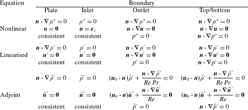
The boundary conditions in table 2 are explained as follows. For the nonlinear Boussinesq equations, the density condition at the plate is derived by assuming a linear relation between density and temperature, and assuming that the plate is a thermal insulator. As usual, the no-slip condition applies. Next, the inlet flow is assumed to be an undisturbed uniform stratified flow. At the outlet, top and bottom, the boundaries are assumed to be far away enough that the flow is essentially uniform in the normal directions. Although this is not analytically true, the associated errors are kept to a minimum by keeping the boundaries very far from the bluff body of interest. Finally, Gresho & Sani (Reference Gresho and Sani1987) argue that it is best to apply the consistent pressure conditions at all boundaries. We apply homogeneous Dirichlet and Neumann conditions respectively at the outlet and the top/bottom, however, to improve the numerical stability.
As aforementioned, the boundary conditions of the linearised equations are the homogeneous versions of the nonlinear conditions. The treatment of the adjoint linearised boundary conditions, however, is more difficult. Analytically, it is sufficient to select conditions on
 $\hat{\unicode[STIX]{x1D70C}}^{\prime }$
,
 $\hat{\boldsymbol{u}}^{\prime }$
and
 $\hat{p}^{\prime }$
such that (2.17), (2.18) are satisfied. It can be verified that the plate, inlet and outlet conditions do in fact satisfy (2.17), (2.18). The top and bottom conditions, however, slightly mismatch the analytical conditions. Nevertheless, we make this selection to achieve better numerical stability, again with the understanding that the top and bottom boundaries are very far from the bluff body.
A.4 Validation
To validate the nonlinear stratified flow solver, we perform three checks. These are – in order – the application an oscillatory localised force, the wavelength of the lee waves and the length of the recirculation bubble.
First, the analytical investigation by Voisin (Reference Voisin1991) shows that when an oscillatory point force is applied in an open stably linearly stratified medium, internal waves are directed diagonally in a pattern known as the St Andrew’s Cross. Specifically, suppose the dimensional angular speed of the oscillation is
 $\tilde{\unicode[STIX]{x1D714}}$
and
 $\tilde{\unicode[STIX]{x1D714}}<{\tilde{N}}$
, where
 ${\tilde{N}}$
is the Brunt–Väisälä frequency as before. Defining the non-dimensional angular speed
 $\unicode[STIX]{x1D714}:=\tilde{\unicode[STIX]{x1D714}}/{\tilde{N}}$
, the waves are oriented at an angle
 $\unicode[STIX]{x1D703}=\cos ^{-1}(\unicode[STIX]{x1D714})$
from the vertical direction. (Voisin assumed an exponential density stratification instead of a linear one, but the differences here are minor.)
Snapshots of the St Andrew’s Cross, shown as
 $\unicode[STIX]{x1D70C}^{\ast }$
(blue:
 $\unicode[STIX]{x1D70C}^{\ast }<0$
; red:
 $\unicode[STIX]{x1D70C}^{\ast }>0$
). The domain shown is
 $[-15.8,15.8]\times [-15.8,15.8]$
. (a)
 $\unicode[STIX]{x1D714}=\sqrt{3}/2$
such that
 $\unicode[STIX]{x1D703}=\unicode[STIX]{x03C0}/6$
; (b)
 $\unicode[STIX]{x1D714}=\sqrt{2}/2$
such that
 $\unicode[STIX]{x1D703}=\unicode[STIX]{x03C0}/4$
; (c)
 $\unicode[STIX]{x1D714}=1/2$
such that
 $\unicode[STIX]{x1D703}=\unicode[STIX]{x03C0}/3$
.

To simulate this experiment, we construct a numerical mesh covering
 $[-200,200]\times [-200,200]$
, with no solid boundaries. The mesh is constructed similarly to figure 18(a), with finer cells near the origin; the mesh contains 213 444 cells. Homogeneous Neumann conditions are applied to
 $\unicode[STIX]{x1D70C}^{\ast }$
,
 $\boldsymbol{u}$
and
 $p^{\ast }$
at all boundaries. For
 $t>0$
, the Gaussian oscillatory forcing term
 $$\begin{eqnarray}\displaystyle \boldsymbol{f}(\boldsymbol{x},t)=\frac{\text{e}^{-\Vert \boldsymbol{x}\Vert ^{2}/2}}{\sqrt{2\unicode[STIX]{x03C0}}}\sin (\unicode[STIX]{x1D714}t) & & \displaystyle\end{eqnarray}$$
is added to the right-hand side of the momentum equation in (A 7). The viscosity is set so that the Womersley number is
 $\unicode[STIX]{x1D6FC}=\tilde{x}_{c}\sqrt{\tilde{\unicode[STIX]{x1D70C}}_{c}\tilde{\unicode[STIX]{x1D714}}/\tilde{\unicode[STIX]{x1D707}}}=10$
, and
 $Pr=7.19$
. In this experiment, the angle of the St Andrew’s Cross is expected to be
 $\unicode[STIX]{x1D703}=\unicode[STIX]{x03C0}/6$
,
 $\unicode[STIX]{x03C0}/4$
, and
 $\unicode[STIX]{x03C0}/3$
respectively for
 $\unicode[STIX]{x1D714}=\sqrt{3}/2$
,
 $\sqrt{2}/2$
, and
 $1/2$
. Figure 19 verifies that the stratified Boussinesq solver reproduces these angles.
Second, we can verify the wavelength of lee waves against basic theory. As discussed in § 3.1, the lee waves should have a wavelength equal to
 $2\unicode[STIX]{x03C0}Fr$
. In our base flows, we find that the lee wavelength is
 $2\unicode[STIX]{x03C0}\cdot 1.00$
for
 $Fr=1$
(figure 1) and
 $2\unicode[STIX]{x03C0}\cdot 8.75$
for
 $Fr=8$
(figure 2). The discrepancy in the latter figure may be because the lee waves are large compared to the mesh boundaries. Regardless, the lee wavelengths are in reasonably good agreement with the analytical theory.
Finally, as a test of sufficient mesh refinement, we compare the recirculation length shown in figure 1 against that of two coarser meshes covering a smaller area. The recirculation length is shown in table 3 and verifies that the current mesh (last row; also figure 18) is sufficient for producing accurate results.
Recirculation lengths with
 $Re=30$
,
 $Pr=7.19$
and
 $Fr=1$
, using different meshes.

Appendix B. Derivation of the Orr–Sommerfeld-type equation
Inserting the wave form of the density and velocity perturbation (4.16) into the linearised continuity and Boussinesq equations (2.13), and using the alternate non-dimensionalisation for density (2.7), (2.8), we obtain
 $$\begin{eqnarray}\displaystyle & \displaystyle 0=\text{i}ku_{a}+\frac{\text{d}v_{a}}{\text{d}y}, & \displaystyle\end{eqnarray}$$
 $$\begin{eqnarray}\displaystyle & \displaystyle \unicode[STIX]{x1D706}\unicode[STIX]{x1D70C}_{a}=-\text{i}ku_{0}\unicode[STIX]{x1D70C}_{a}-\frac{\text{d}\unicode[STIX]{x1D70C}_{0}}{\text{d}y}v_{a}+\frac{1}{Re\,Pr}\left(\frac{\text{d}^{2}}{\text{d}y^{2}}-k^{2}\right)\unicode[STIX]{x1D70C}_{a}, & \displaystyle\end{eqnarray}$$
 $$\begin{eqnarray}\displaystyle & \displaystyle \unicode[STIX]{x1D706}u_{a}\text{e}^{\text{i}kx+\unicode[STIX]{x1D706}t}=\left(-\text{i}ku_{0}u_{a}-\frac{\text{d}u_{0}}{\text{d}y}v_{a}+\frac{1}{Re}\left(\frac{\text{d}^{2}}{\text{d}y^{2}}-k^{2}\right)u_{a}\right)\text{e}^{\text{i}kx+\unicode[STIX]{x1D706}t}-\frac{\unicode[STIX]{x2202}p^{\prime }}{\unicode[STIX]{x2202}x}, & \displaystyle\end{eqnarray}$$
 $$\begin{eqnarray}\displaystyle & \displaystyle \unicode[STIX]{x1D706}v_{a}\text{e}^{\text{i}kx+\unicode[STIX]{x1D706}t}=\left(-\text{i}ku_{0}v_{a}+\frac{1}{Re}\left(\frac{\text{d}^{2}}{\text{d}y^{2}}-k^{2}\right)v_{a}-\frac{\unicode[STIX]{x1D70C}_{a}}{Fr^{2}}\right)\text{e}^{\text{i}kx+\unicode[STIX]{x1D706}t}-\frac{\unicode[STIX]{x2202}p^{\prime }}{\unicode[STIX]{x2202}y}. & \displaystyle\end{eqnarray}$$
 $x$
-derivative of (B 1d
) from the
 $y$
-derivative of (B 1c
) yields
 $$\begin{eqnarray}\displaystyle \unicode[STIX]{x1D706}\left(\frac{\text{d}u_{a}}{\text{d}y}-\text{i}kv_{a}\right) & = & \displaystyle -\text{i}k\left(\frac{\text{d}u_{0}}{\text{d}y}u_{a}+u_{0}\frac{\text{d}u_{a}}{\text{d}y}\right)-\frac{\text{d}^{2}u_{0}}{\text{d}y^{2}}v_{a}-\frac{\text{d}u_{0}}{\text{d}y}\frac{\text{d}v_{a}}{\text{d}y}-k^{2}u_{0}v\nonumber\\ \displaystyle & & \displaystyle +\,\frac{1}{Re}\left(\frac{\text{d}^{2}}{\text{d}y^{2}}-k^{2}\right)\left(\frac{\text{d}u_{a}}{\text{d}y}-\text{i}kv_{a}\right)+\frac{\text{i}k\unicode[STIX]{x1D70C}_{a}}{Fr^{2}}.\end{eqnarray}$$
Using (B 1a
) to eliminate
 $u_{a}$
yields
 $$\begin{eqnarray}\displaystyle \frac{\text{i}\unicode[STIX]{x1D706}}{k}\left(\frac{\text{d}^{2}}{\text{d}y^{2}}-k^{2}\right)v_{a}=-\frac{\text{d}^{2}u_{0}}{\text{d}y^{2}}v_{a}+u_{0}\left(\frac{\text{d}^{2}}{\text{d}y^{2}}-k^{2}\right)v_{a}+\frac{\text{i}}{kRe}\left(\frac{\text{d}^{2}}{\text{d}y^{2}}-k^{2}\right)^{2}v_{a}+\frac{\text{i}k\unicode[STIX]{x1D70C}_{a}}{Fr^{2}}. & & \displaystyle \nonumber\\ \displaystyle & & \displaystyle\end{eqnarray}$$
The combination of (B 1b
) and the product of the above with
 $-\text{i}k$
yields (4.17) and (4.18).
To derive the boundary conditions (4.19), we observe from table 2 that the top and bottom conditions on
 $\unicode[STIX]{x1D70C}^{\prime }$
and
 $v^{\prime }$
immediately imply homogeneous Neumann conditions on
 $\unicode[STIX]{x1D70C}_{a}$
and
 $v_{a}$
. From (B 1a
), we can then observe that the top and bottom conditions on
 $u^{\prime }$
are equivalent to
 $\text{d}^{2}v_{a}/\text{d}y^{2}=0$
.
The derivation of the Orr–Sommerfeld-type equation for the adjoint linearised Boussinesq equation (2.16) proceeds exactly analogously. Inserting the wave form (4.20) into the continuity and momentum equations yields
 $$\begin{eqnarray}\displaystyle & \displaystyle 0=\text{i}k\hat{u} _{a}+\frac{\text{d}\hat{v}_{a}}{\text{d}y}, & \displaystyle\end{eqnarray}$$
 $$\begin{eqnarray}\displaystyle & \displaystyle \bar{\unicode[STIX]{x1D706}}\hat{\unicode[STIX]{x1D70C}}_{a}=\text{i}ku_{0}\hat{\unicode[STIX]{x1D70C}}_{a}+\frac{1}{Re\,Pr}\left(\frac{\text{d}^{2}}{\text{d}y^{2}}-k^{2}\right)\hat{\unicode[STIX]{x1D70C}}_{a}-\frac{\hat{v}_{a}}{Fr^{2}}, & \displaystyle\end{eqnarray}$$
 $$\begin{eqnarray}\displaystyle & \displaystyle \bar{\unicode[STIX]{x1D706}}\hat{u} _{a}\text{e}^{\text{i}kx+\bar{\unicode[STIX]{x1D706}}t}=\left(\text{i}ku_{0}\hat{u} _{a}+\frac{1}{Re}\left(\frac{\text{d}^{2}}{\text{d}y^{2}}-k^{2}\right)\hat{u} _{a}\right)\text{e}^{\text{i}kx+\bar{\unicode[STIX]{x1D706}}t}-\frac{\unicode[STIX]{x2202}\hat{p}^{\prime }}{\unicode[STIX]{x2202}x}, & \displaystyle\end{eqnarray}$$
 $$\begin{eqnarray}\displaystyle & \displaystyle \bar{\unicode[STIX]{x1D706}}\hat{v}_{a}\text{e}^{\text{i}kx+\bar{\unicode[STIX]{x1D706}}t}=\left(-\frac{\text{d}\unicode[STIX]{x1D70C}_{0}}{\text{d}y}\hat{\unicode[STIX]{x1D70C}}_{a}-\frac{\text{d}u_{0}}{\text{d}y}\hat{u} _{a}+\text{i}ku_{0}\hat{v}_{a}+\frac{1}{Re}\left(\frac{\text{d}^{2}}{\text{d}y^{2}}-k^{2}\right)\hat{v}_{a}\right)\text{e}^{\text{i}kx+\bar{\unicode[STIX]{x1D706}}t}-\frac{\unicode[STIX]{x2202}\hat{p}^{\prime }}{\unicode[STIX]{x2202}y}.\qquad & \displaystyle\end{eqnarray}$$
 $x$
-derivative of (B 4d
) from the
 $y$
-derivative of (B 4c
) yields
 $$\begin{eqnarray}\displaystyle \bar{\unicode[STIX]{x1D706}}\left(\frac{\text{d}\hat{u} _{a}}{\text{d}y}-\text{i}k\hat{v}_{a}\right) & = & \displaystyle \text{i}k\left(2\frac{\text{d}u_{0}}{\text{d}y}\hat{u} _{a}+u_{0}\frac{\text{d}\hat{u} _{a}}{\text{d}y}+\frac{\text{d}\unicode[STIX]{x1D70C}_{0}}{\text{d}y}\hat{\unicode[STIX]{x1D70C}}_{a}\right)+k^{2}u_{0}\hat{v}_{a}\nonumber\\ \displaystyle & & \displaystyle +\,\frac{1}{Re}\left(\frac{\text{d}^{2}}{\text{d}y^{2}}-k^{2}\right)\left(\frac{\text{d}\hat{u} _{a}}{\text{d}y}-\text{i}k\hat{v}_{a}\right),\end{eqnarray}$$
and using (B 4a
) to eliminate
 $\hat{u} _{a}$
yields
 $$\begin{eqnarray}\displaystyle \frac{\text{i}\bar{\unicode[STIX]{x1D706}}}{k}\left(\frac{\text{d}^{2}}{\text{d}y^{2}}-k^{2}\right)v_{a} & = & \displaystyle -2\frac{\text{d}u_{0}}{\text{d}y}\frac{\text{d}\hat{v}_{a}}{\text{d}y}-u_{0}\left(\frac{\text{d}^{2}}{\text{d}y^{2}}-k^{2}\right)\hat{v}_{a}+\text{i}k\frac{\text{d}\unicode[STIX]{x1D70C}_{0}}{\text{d}y}\hat{\unicode[STIX]{x1D70C}}_{a}\nonumber\\ \displaystyle & & \displaystyle +\,\frac{\text{i}}{kRe}\left(\frac{\text{d}^{2}}{\text{d}y^{2}}-k^{2}\right)^{2}\hat{v}_{a}.\end{eqnarray}$$
Finally, the combination of (B 4b
) and the product of the above with
 $-\text{i}k$
yields (4.21) and (4.22).
In deriving the boundary conditions for (4.23), we recall that
 $\boldsymbol{u}_{0}\boldsymbol{\cdot }\boldsymbol{n}=0$
at the top and bottom boundaries. Therefore, for parallel base flows, the conditions for the full adjoint linearised Boussinesq equations (table 2) are essentially of homogeneous Neumann type on the top and bottom boundaries. As before, we recover homogeneous Neumann conditions for
 $\hat{\unicode[STIX]{x1D70C}}_{a}$
and
 $\hat{v}_{a}$
, and (B 4a
) then implies
 $\text{d}^{2}\hat{v}_{a}/\text{d}y^{2}=0$
.