2 Proof of Theorem 1

Suppose that $\mathcal {S}$ is a measurable subset of the plane such that ${\text {area}}(\mathcal {S})=\infty $ . The first step of the proof is to locate a triangle $\triangle ABC$ of area $1$ with vertices in $\mathcal {S}$ in a way that we also have control over its angles and over the density of $\mathcal {S}$ at C. The argument is a modification of the standard one mentioned in the introduction [Reference Croft, Falconer and Guy4, p. 182].

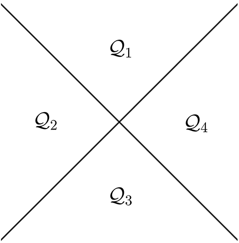
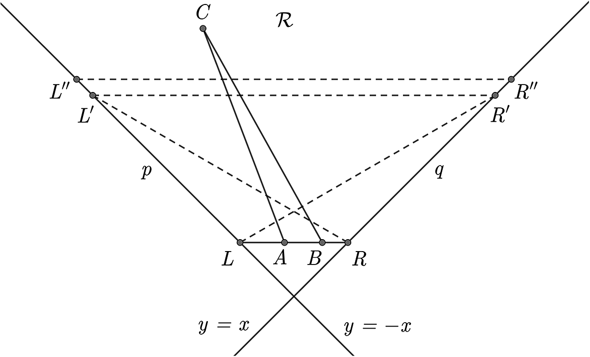
Consider a pair of orthogonal lines p and q in the plane. They subdivide the plane (up to negligible sets) into four closed right-angled sectors (i.e., quadrants) $\mathcal {Q}_{1},\mathcal {Q}_{2},\mathcal {Q}_{3},\mathcal {Q}_{4}$ , as in Figure 1. By pigeonholing, there exists some $1\leqslant i\leqslant 4$ such that ${\text {area}}(\mathcal {S}\cap \mathcal {Q}_{i}) =\infty $ . Choosing the coordinate system so that $\mathcal {Q}_i$ becomes the “upper” sector, we can write

$$\begin{align*}\mathcal{Q}_i = \{ (x,y)\in\mathbb{R}^2 \,:\, y\geqslant |x| \} \end{align*}$$

and then the lines p and $q,$ respectively, have Cartesian equations $y=-x$ and $y=x$ (see Figure 2). For every $t\geqslant 0$ denote the points $L_{t}=(-t,t)$ and $R_{t} = (t,t)$ , so that the family of line segments $\overline {L_{t}R_{t}}$ indexed by $t\geqslant 0$ partitions $\mathcal {Q}_{i}$ . By Fubini’s theorem,

$$\begin{align*}{\text{area}}(\mathcal{S}\cap\mathcal{Q}_{i}) =\int_{0}^{\infty} {\text{length}}\big(\mathcal{S}\cap\overline{L_{t}R_{t}}\big) \,\text{d}t. \end{align*}$$

Therefore, there has to exist some $t>0$ such that the one-dimensional Lebesgue measure of $\mathcal {S}\cap \overline {L_{t}R_{t}}$ is strictly positive. From now on, we fix one particular such t and denote $L=L_t$ and $R=R_t$ . Define

$$\begin{align*}\mathcal{I} := \big\{ x\in\mathbb{R} \,:\, (x,t) \in \mathcal{S}\cap\overline{LR} \big\} \subseteq [-t,t]. \end{align*}$$

By the Steinhaus theorem [Reference Steinhaus13], the fact ${\text {length}}(\mathcal {I})>0$ implies that there exists some $\theta>0$ such that the difference set $\mathcal {I}-\mathcal {I}$ contains the interval $(-\theta ,\theta )$ . Thus, for any $0<c<\theta $ , we can find two points in $\mathcal {S}\cap \overline {LR}$ at distance precisely c apart from each other.

Figure 1

Quadrants.

Figure 2

Locating $\triangle ABC$ .

Figure 2 Long description

A geometric line drawing on a coordinate plane. At the bottom, two solid lines intersect at an origin point, labeled y equals x for the line rising to the right and y equals minus x for the line rising to the left.

Above the intersection, a horizontal line segment connects point L on the left line to point R on the right line. Between L and R are points A and B.

From point L, a solid line labeled p extends upward and to the left, containing points L prime and L double prime. From point R, a solid line labeled q extends upward and to the right, containing points R prime and R double prime.

Triangle A B C is formed by vertex C at the top left and base segment A B. Solid lines connect C to A and C to B.

Dashed lines show geometric relationships. A horizontal dashed line connects L double prime to R double prime, and another connects L prime to R prime. Diagonal dashed lines connect L to R prime and R to L prime.

The region above the horizontal segment L R is labeled with a calligraphic R.

Let $L'$ on p and $R'$ on q be the points such that $\angle L'RL = 30^\circ $ and $\angle RLR' = 30^\circ $ . Next, let $L"$ on p and $R"$ on q be such that $L"R"$ is parallel to $L'R'$ and lies above (or coincides with) line $L'R'$ , and that the distance between the lines $LR$ and $L"R"$ is at least $2/\theta $ . Finally, let $\mathcal {R}$ be the unbounded open region the boundary of which consists of p, q, and $L"R"$ (see Figure 2 again). Note that we still have ${{\text {area}}(\mathcal {S}\cap \mathcal {R})=\infty }$ , but from now on, we only need ${\text {area}}(\mathcal {S}\cap \mathcal {R})>0$ . Almost every point of $\mathcal {S}\cap \mathcal {R}$ is its Lebesgue density point (see, e.g., [Reference Stein and Weiss12, p. 12] or [Reference Folland8, Theorem 3.21]), so there exists a point C in that set such that

$$\begin{align*}\lim_{ \varepsilon \to 0^+ } \frac{{\text{area}}(\mathcal{S} \cap \mathcal{D}_{\varepsilon}(C))}{{\text{area}}(\mathcal{D}_{\varepsilon}(C))} = 1. \end{align*}$$

In particular, there exists $\varepsilon _1>0$ such that

(2.1) $$ \begin{align} \frac{{\text{area}}(\mathcal{S} \cap \mathcal{D}_{\varepsilon}(C))}{{\text{area}}(\mathcal{D}_{\varepsilon}(C))}> \frac{9999}{10000} \quad\text{for every } \varepsilon\in(0,\varepsilon_1]. \end{align} $$

Now, let $c\in (0,\theta )$ be such that the distance from the point C to the line $LR$ is precisely $2/c$ . From the conclusion of the previous paragraph, we can find points $A,B\in \mathcal {S}\cap \overline {LR}$ such that $|AB|=c$ . The area of $\triangle ABC$ is then clearly $1$ , while its angles satisfy

$$\begin{align*}\angle CBA \geqslant \angle CRL> \angle L'RL = 30^\circ \end{align*}$$

and

$$\begin{align*}\angle CAB \geqslant \angle CLR> \angle R'LR = 30^\circ. \end{align*}$$

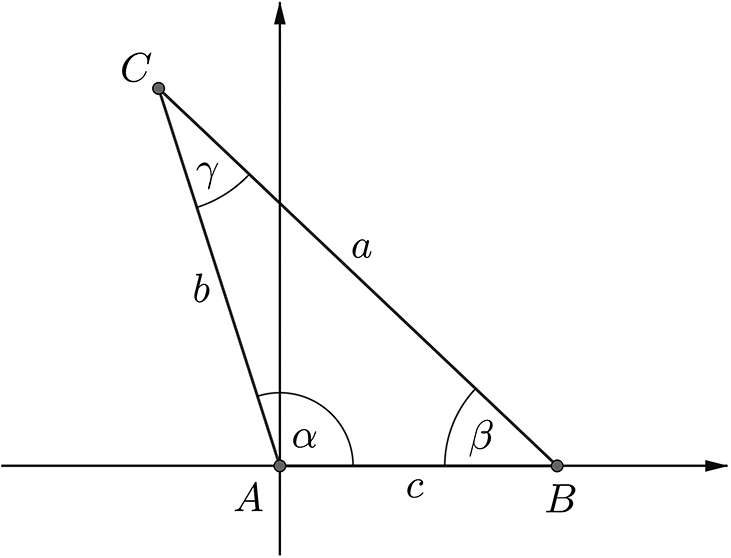
We regard the positively oriented triangle $\triangle ABC$ as fixed and find it advantageous to change the coordinate system, by placing the origin at A and putting B on the positive part of the x-axis. The new coordinates of the vertices of $\triangle ABC$ become

$$\begin{align*}A=(0,0), \ B=(c,0), \ C=(x_{C},y_{C}) \end{align*}$$

for some $x_C\in \mathbb {R}$ and $y_C>0$ . Lengths of its sides will be written

$$\begin{align*}a=|BC|, \ b=|CA|, \ c=|AB| \end{align*}$$

and its angles will be denoted standardly as

$$\begin{align*}\alpha=\angle BAC, \ \beta=\angle CBA, \ \gamma=\angle ACB; \end{align*}$$

see Figure 3. Recall that we have shown

(2.2) $$ \begin{align} 30^\circ < \alpha,\beta < 150^\circ. \end{align} $$

Figure 3

Triangle elements.

The proof proceeds by “perturbing” the point C slightly to locate $D,E$ in its small neighborhood such that $ABED$ is a non-degenerate cyclic quadrilateral of area $1$ . To achieve this, we need to study analytical properties of the assignment $D\mapsto E$ , which finds a unique appropriate point E for many initial choices of D, and we only care about the cases when D and E are sufficiently close to C. Since the set $\mathcal {S}$ is “very dense” around C, it will not be able to miss all such pairs $(D,E)$ .

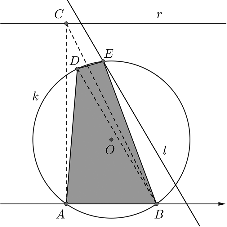
The reason why we restrict ourselves to the half-disk $\mathcal {D}^{-}_{\varrho }(C)$ is that $D,A,B$ cannot be consecutive vertices of an area $1$ cyclic quadrilateral if D lies on or above the line r passing through C and parallel to the x-axis (see Figure 4).

Figure 4

Map $f\colon D\mapsto E$ .

Figure 4 Long description

A geometric construction is presented. At the top, a horizontal line labeled r contains a point C. A circle labeled k with center O is positioned in the middle of the frame. A shaded gray quadrilateral is formed by vertices A, B, E, and D. Points A and B lie on a horizontal axis at the bottom of the circle. Points D and E lie on the upper arc of the circle k.

Several dashed lines connect point C to other vertices. A vertical dashed line connects C to A. Two diagonal dashed lines connect C to D and C to B. A solid line labeled l passes through point E and intersects the bottom horizontal axis to the right of point B. Another solid line passes through point C and point E, extending diagonally across the circle. The diagram illustrates the spatial relationship between the linear projection from point C and the resulting inscribed area within the circle.

Proof We will use the implicit function theorem to obtain the existence of the desired function $f\colon D\mapsto E$ , defined locally, in a neighborhood of C, from a system of two equations in two variables, which encode the geometric requirements, i.e., that the quadrilateral $ABED$ is cyclic and has area $1$ . We regard D as fixed and try to locate the point $E=f(D)$ . Introduce the Cartesian coordinates of the two points,

$$\begin{align*}D=(x_{D},y_{D}), \ E=(x_{E},y_{E}). \end{align*}$$

Using the so-called “shoelace formula” for the area in the Cartesian plane, we easily obtain

$$\begin{align*}\frac{1}{2} \big( 0 \cdot 0 - c \cdot 0 + c \cdot y_E - x_E \cdot 0 + x_E \cdot y_D - x_D \cdot y_E + x_D \cdot 0 - 0 \cdot y_D \big) = 1, \end{align*}$$

i.e.,

(2.7) $$ \begin{align} y_{D}x_{E} + (c-x_{D})y_{E} - 2 = 0 \end{align} $$

holds whenever $ABED$ is a quadrilateral of area $1$ . We conclude that E needs to lie on the line l given by the equation

(2.8) $$ \begin{align} y_D x + (c-x_D) y - 2 =0; \end{align} $$

see Figure 4.

Furthermore, we require that the points $A,B,E,D$ are concyclic. In order to find the equation of the circumcircle k of the triangle $\triangle ABD$ , we observe that its center $O(x_O,y_O)$ lies on the perpendicular bisectors of the sides $\overline {AB}$ and $\overline {AD}$ , which are, respectively, given by

$$\begin{align*}x=\frac{c}{2}, \quad y=-\frac{x_{D}}{y_{D}}\Big(x-\frac{x_{D}}{2}\Big) + \frac{y_{D}}{2}. \end{align*}$$

Solving this system gives

$$\begin{align*}(x_O,y_O) = \Big( \frac{c}{2}, \frac{x_D^2 + y_D^2 - cx_D}{2y_D} \Big), \end{align*}$$

while the equation of circle k reads

$$\begin{align*}(x-x_O)^2 + (y-y_O)^2 = x_O^2 + y_O^2. \end{align*}$$

Plugging $(x,y)=(x_{E},y_{E})$ into the last equation and simplifying, we obtain

(2.9) $$ \begin{align} x_{E}^2 + y_{E}^2 - cx_{E} + \frac{c x_{D} - x_{D}^2 - y_{D}^2}{y_{D}}y_{E} = 0. \end{align} $$

The point E lies at the intersection of l and k (see Figure 4 again), so its coordinates $x_E,y_E$ need to satisfy both equations (2.7) and (2.9).

Motivated by (2.7) and (2.9), we consider the function

$$\begin{align*}\Phi\colon\mathbb{R}\times(0,\infty)\times\mathbb{R}^2 \to \mathbb{R}^2, \end{align*}$$

defined by

$$\begin{align*}\Phi(x_1,y_1,x_2,y_2) = \Big( y_1 x_2 + (c-x_1) y_2 - 2, \ x_2^2 + y_2^2 - cx_2 + \frac{c x_1 - x_1^2 - y_1^2}{y_1}y_2 \Big). \end{align*}$$

Note that ${\text {area}}(\triangle ABC) = 1$ can be rewritten as $cy_C=2$ , which easily implies

(2.10) $$ \begin{align} \Phi(C,C) = \Phi(x_{C},y_{C},x_{C},y_{C}) = (cy_C-2, 0) = (0,0). \end{align} $$

Furthermore, we calculate the differential in the first two variables $(x_1,y_1)$ at $(C,C)$ as

$$\begin{align*}\text{d}_{1}\Phi(C,C) =\begin{bmatrix} -y_{C} & x_{C} \\ c-2x_{C} & \frac{x_{C}^2 - cx_{C} - y_{C}^2}{y_{C}} \end{bmatrix} \end{align*}$$

and the differential in the last two variables $(x_2,y_2)$ at $(C,C)$ as

$$\begin{align*}\text{d}_{2}\Phi(C,C) =\begin{bmatrix} y_{C} & c-x_{C} \\ 2x_{C} - c & \frac{- x_{C}^2 + cx_{C} + y_{C}^2}{y_{C}} \end{bmatrix}. \end{align*}$$

Note that the determinant of the latter operator,

$$\begin{align*}\det \text{d}_{2}\Phi(C,C) = (x_{C}-c)^2 + y_{C}^2, \end{align*}$$

is strictly positive because of $y_{C}>0$ ; in particular, it is nonzero. Applying the implicit function theorem, we obtain open neighborhoods $\mathcal {U}',\mathcal {V}' \subseteq \mathcal {R}$ of the point C such that there exists a unique function $f\colon \mathcal {U}'\to \mathcal {V}'$ satisfying

(2.11) $$ \begin{align} \Phi(D,E) = 0 \ \Longleftrightarrow\ E=f(D) \end{align} $$

for every $D\in \mathcal {U}'$ and $E\in \mathcal {V}'$ . In particular, a consequence of (2.10) is $f(C)=C$ . Furthermore, the implicit function theorem also guarantees that f is continuously differentiable and its differential can be computed by the formula

$$\begin{align*}\text{d}f(C) = - \big(\text{d}_{2}\Phi(C,C)\big)^{-1} \text{d}_{1}\Phi(C,C). \end{align*}$$

After some calculation using the above expressions for $\text {d}_{1}\Phi (C,C)$ and $\text {d}_{2}\Phi (C,C)$ , we obtain

$$\begin{align*}\text{d}f(C) = -\frac{1}{(x_{C}-c)^2 + y_{C}^2}\begin{bmatrix} \frac{-x_{C}^2+cx_{C}+y_{C}^2}{y_{C}} & x_{C}-c \\ c-2x_{C} & y_{C} \end{bmatrix} \begin{bmatrix} -y_{C} & x_{C} \\ c-2x_{C} & \frac{x_{C}^2 - cx_{C} - y_{C}^2}{y_{C}} \end{bmatrix}, \end{align*}$$

i.e.,

$$\begin{align*}\text{d}f(C) = \begin{bmatrix} 1 & \frac{c(x_{C}^2 - cx_{C} - y_{C}^2)}{((x_C-c)^2+y_C^2) y_{C}} \\[2mm] 0 & \frac{x_C^2+y_C^2}{(x_C-c)^2+y_C^2} \end{bmatrix}. \end{align*}$$

Using

$$\begin{align*}x_C^2+y_C^2 = b^2, \quad (x_C-c)^2+y_C^2 = a^2, \end{align*}$$

which is clear from Figure 3, we simplify $\text {d}f(C)$ as

$$\begin{align*}\text{d}f(C) = \begin{bmatrix} 1 & \frac{c(x_{C}^2 - cx_{C} - y_{C}^2)}{a^2 y_{C}} \\[2mm] 0 & \frac{b^2}{a^2} \end{bmatrix} \end{align*}$$

and then the sine theorem for $\triangle ABC$ and some trigonometric manipulation easily yield the desired formula (2.6).

Since $\det \text {d}f(C) \neq 0$ , we can apply the inverse function theorem to obtain open neighborhoods $\mathcal {U}\subseteq \mathcal {U}'$ and $\mathcal {V}\subseteq \mathcal {V}'$ of the point C such that $f\colon \mathcal {U} \to \mathcal {V}$ is a $\text {C}^1$ -diffeomorphism. By further shrinking, we can assume that $\mathcal {U}$ is an open disk $\mathcal {D}_{\varrho }(C)$ of some radius $\varrho>0$ . Besides the notation introduced in the lemma statement, also denote

$$ \begin{align*} \mathcal{D}^{+}_{\varrho}(C) & := \{(x,y)\in\mathcal{D}_{\varrho}(C) \,:\, y>y_C\}, \\ \mathcal{D}^{0}_{\varrho}(C) & := \{(x,y)\in\mathcal{D}_{\varrho}(C) \,:\, y=y_C\}, \\ \mathcal{V}^{+} & := \{(x,y)\in\mathcal{V} \,:\, y>y_C\}, \\ \mathcal{V}^{0} & := \{(x,y)\in\mathcal{V} \,:\, y=y_C\}. \end{align*} $$

For every $D\in \mathcal {D}^{-}_{\varrho }(C)$ , the first part of the proof and (2.11) guarantee that $E=f(D)$ is the unique point lying both on the circle k through $A,B,D$ and the line l defined by (2.8). Since D is below the line r, which means ${\text {area}}(\triangle ABD)<1$ , the points on the circle k really appear in the order $A,B,E,D$ and form a cyclic quadrilateral of area $1$ . Moreover, ${\text {area}}(\triangle ABE)<{\text {area}}(\triangle ABED)$ , so E is also below the line r, i.e., $E\in \mathcal {D}^{-}_{\varrho }(C)$ . This proves $f(\mathcal {D}^{-}_{\varrho }(C))\subseteq \mathcal {V}^{-}$ and tentatively also (2.5) provided that we can show the equality in this last set inclusion, i.e., that (2.4) holds.

Next, we claim that for every $D\in \mathcal {D}_{\varrho }(C),$ one has

(2.12) $$ \begin{align} D \in r \ \Longleftrightarrow\ E=f(D) \in r. \end{align} $$

In fact, (2.12) then further implies $E=D$ , but we do not need that in the following text. Even if this claim is geometrically evident, we give its rigorous analytical proof. Namely, the definition of f guarantees $\Phi (x_D,y_D,x_E,y_E)=(0,0)$ provided that ${E=f(D)}$ , and the equality of the first coordinates yields

(2.13) $$ \begin{align} y_D x_E + (c-x_D) y_E = 2 = c y_C, \end{align} $$

which enables us to express $x_E$ in terms of $x_D$ , $y_D$ , and $y_E$ . Now, if $y_D=y_C$ , then the second equality simplifies, after some calculation, as

$$\begin{align*}(y_E - y_C) \underbrace{y_E \big( (x_D-c)^2 + y_C^2 \big)}_{>0} = 0, \end{align*}$$

which implies $y_E=y_C$ . Conversely, if $y_E=y_C$ , then the second inequality easily reduces to

$$\begin{align*}(y_D-y_C) \underbrace{y_C (x_D^2+y_D^2)}_{>0} = 0, \end{align*}$$

which gives $y_D=y_C$ . (After we conclude $y_C=y_D=y_E$ , then (2.13) also implies ${x_E=x_D}$ , so that we indeed have $E=D$ .) Note that (2.12) can be equivalently written as $f(\mathcal {D}^{0}_{\varrho }(C))=\mathcal {V}^{0}$ .

Finally, the continuity of f and the connectedness of $\mathcal {D}^{+}_{\varrho }(C)$ imply ${f(\mathcal {D}^{+}_{\varrho }(C)){\kern-1pt}\subseteq{\kern-1pt} \mathcal {V}^{+}}$ . From all this, we conclude that the image $f(\mathcal {D}^{-}_{\varrho }(C))$ needs to be precisely equal to $\mathcal {V}^{-}$ .

Estimating the operator norm of $\text {d}f(C)$ by the $\ell ^2$ -norm of its matrix entries (the so-called Frobenius matrix norm), from (2.6) and (2.2), we get

$$ \begin{align*} \|\text{d}f(C)\|_{\text{op}} & \stackrel{({2.6})}{\leqslant} \sqrt{1^2 + \bigg(\frac{(\cos 2\alpha \sin\beta - \cos\alpha \sin\gamma)\sin\gamma}{\sin^3\alpha}\bigg)^2 + \Big(\frac{\sin^2\beta}{\sin^2\alpha}\Big)^2} \\ & \stackrel{({2.2})}{\leqslant} \sqrt{1 + \Big(\frac{2}{\sin^3 30^\circ}\Big)^2 + \Big(\frac{1}{\sin^2 30^\circ}\Big)^2} < 20. \end{align*} $$

Also,

$$\begin{align*}\det(\text{d}f(C)) \stackrel{({2.6})}{=} \frac{\sin^2\beta}{\sin^2\alpha} \stackrel{({2.2})}{\geqslant} \sin^2 30^\circ = \frac{1}{4}. \end{align*}$$

By continuity of the maps,

$$\begin{align*}P \mapsto \|\text{d}f(P)\|_{\text{op}} \quad\text{and}\quad P \mapsto \det(\text{d}f(P)), \end{align*}$$

there exists $0<\varepsilon _2\leqslant \varrho $ such that

(2.14) $$ \begin{align} \|\text{d}f(P)\|_{\text{op}} <20 \quad\text{for every } P\in\mathcal{D}_{\varepsilon_2}(C) \end{align} $$

and

(2.15) $$ \begin{align} \det(\text{d}f(P))>\frac{1}{5} \quad\text{for every } P\in\mathcal{D}_{\varepsilon_2}(C). \end{align} $$

Next, by the mean value inequality for vector-valued functions, we conclude that

$$\begin{align*}|Cf(P)| \stackrel{({2.3})}{=} |f(C)f(P)| \stackrel{({2.14})}{\leqslant} 20 |CP| \end{align*}$$

holds for every $P\in \mathcal {D}_{\varepsilon _2}(C)$ , so

(2.16) $$ \begin{align} f(\mathcal{D}_{\varepsilon}(C)) \subseteq \mathcal{D}_{20\varepsilon}(C) \quad\text{for every } \varepsilon\in(0,\varepsilon_2]. \end{align} $$

Let $\mathcal {D}_{\varepsilon _3}(C)$ , for some $\varepsilon _3>0$ , be a disk around C fully contained in $\mathcal {V}$ .

From (2.1), we conclude

$$\begin{align*}\frac{1}{2}\cdot\frac{{\text{area}}(\mathcal{S} \cap \mathcal{D}^{-}_{\varepsilon}(C))}{{\text{area}}(\mathcal{D}^{-}_{\varepsilon}(C))} + \frac{1}{2}\cdot\underbrace{\frac{{\text{area}}(\mathcal{S} \cap \mathcal{D}^{+}_{\varepsilon}(C))}{{\text{area}}(\mathcal{D}^{+}_{\varepsilon}(C))}}_{\leqslant1} \stackrel{({2.1})}{>} \frac{9999}{10000} \end{align*}$$

whenever $\varepsilon \leqslant \varepsilon _1$ , so that

(2.17) $$ \begin{align} \frac{{\text{area}}(\mathcal{S} \cap \mathcal{D}^{-}_{\varepsilon}(C))}{{\text{area}}(\mathcal{D}^{-}_{\varepsilon}(C))}> \frac{4999}{5000} \quad\text{for every } \varepsilon\in(0,\varepsilon_1]. \end{align} $$

Finally, take

$$\begin{align*}\delta := \min\{\varepsilon_1,\varepsilon_2,\varepsilon_3\} \end{align*}$$

and define the set

$$\begin{align*}\mathcal{A} := \mathcal{S} \cap \mathcal{D}^{-}_{\delta}(C), \end{align*}$$

so that (2.17) immediately gives

$$\begin{align*}{\text{area}}(\mathcal{A})> \frac{4999}{5000} {\text{area}}(\mathcal{D}^{-}_{\delta}(C)). \end{align*}$$

Also define

$$\begin{align*}\mathcal{B} := f\big(\mathcal{S} \cap \mathcal{D}^{-}_{\delta/20}(C)\big), \end{align*}$$

so that (2.4) and (2.16) guarantee $\mathcal {B}\subseteq \mathcal {D}^{-}_{\delta }(C)$ , while the change of variables formula (e.g., [Reference Folland8, Theorem 2.47]), the fact that f is $\text {C}^1$ -diffeomorphism, (2.15) and (2.17) give

$$ \begin{align*} {\text{area}}(\mathcal{B}) & = \int_{\mathcal{S} \cap \mathcal{D}^{-}_{\delta/20}(C)} |\det(\text{d}f(P))| \,\text{d}P \stackrel{({2.15})}{\geqslant} \frac{1}{5}{\text{area}}\big(\mathcal{S} \cap \mathcal{D}^{-}_{\delta/20}(C)\big) \\ & \stackrel{({2.17})}{>} \frac{1}{5} \cdot\frac{4999}{5000}\cdot \frac{1}{20^2} {\text{area}}(\mathcal{D}^{-}_{\delta}(C)) > \frac{1}{5000}{\text{area}}(\mathcal{D}^{-}_{\delta}(C)). \end{align*} $$

Therefore, $\mathcal {A}$ and $\mathcal {B}$ are two measurable subsets of $\mathcal {D}^{-}_{\delta }(C)$ satisfying

$$\begin{align*}{\text{area}}(\mathcal{A}) + {\text{area}}(\mathcal{B})> {\text{area}}(\mathcal{D}^{-}_{\delta}(C)), \end{align*}$$

so they cannot be disjoint. Let E be a point from the intersection $\mathcal {A}\cap \mathcal {B}$ . By the definition of $\mathcal {A,}$ we have $E\in \mathcal {S} \cap \mathcal {D}^{-}_{\varepsilon _3}(C)\subseteq \mathcal {S}\cap \mathcal {V}^{-}$ , while the definition of $\mathcal {B}$ gives a point $D\in \mathcal {S}\cap \mathcal {D}^{-}_{\varrho }(C)$ such that $E=f(D)$ . Now, we know that $A,B,D,E\in \mathcal {S}$ and (2.5) finalizes the proof of Theorem 1 by concluding that $ABED$ is a cyclic quadrilateral of unit area.

3 Proof of Theorem 2

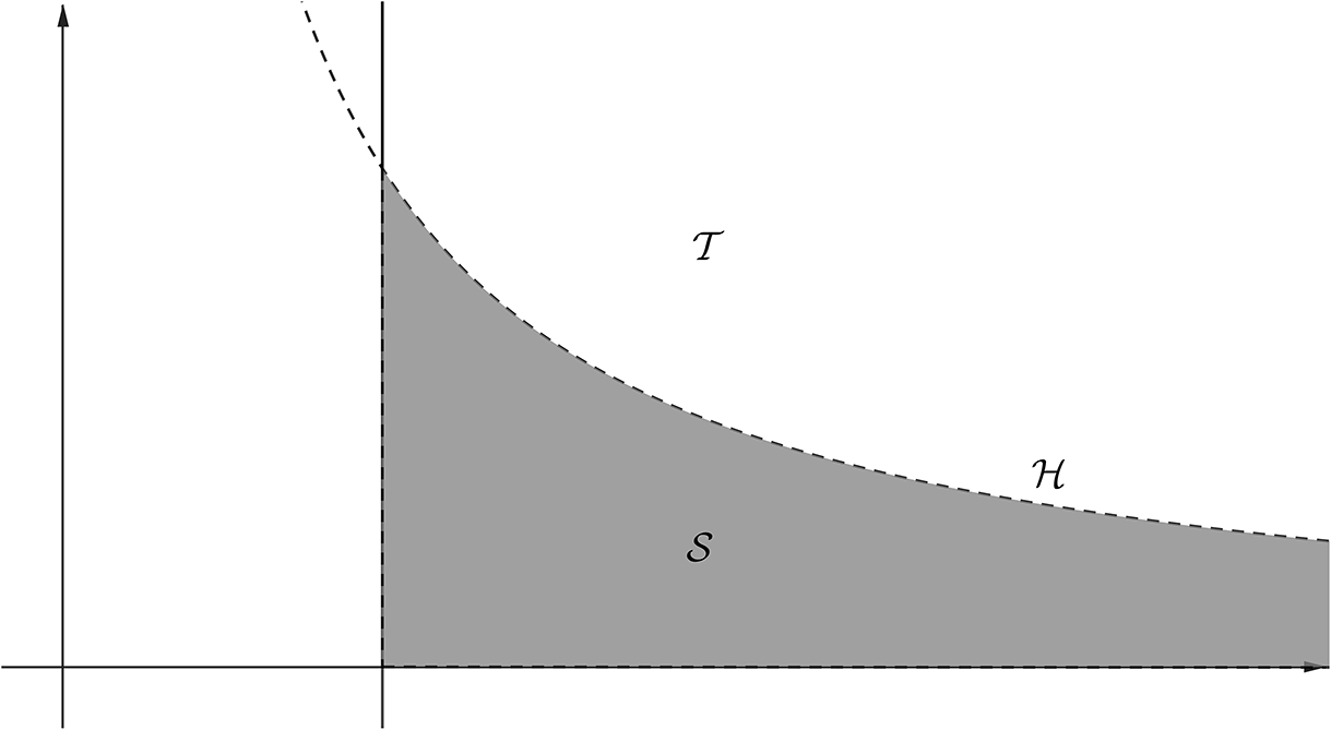
An example of a set with the desired property is

$$\begin{align*}\mathcal{S} := \{ (x,y)\in\mathbb{R}^2 \,:\, x>1,\, y>0,\, 4xy<1 \}. \end{align*}$$

Its upper boundary is a piece of hyperbola,

$$\begin{align*}\mathcal{H} := \{ (x,y)\in\mathbb{R}^2 \,:\, x>1,\, 4xy=1 \}, \end{align*}$$

which is, at the same time, the lower boundary of the closed convex set

$$\begin{align*}\mathcal{T} := \{ (x,y)\in\mathbb{R}^2 \,:\, x\geqslant1,\, 4xy\geqslant1 \}; \end{align*}$$

see Figure 5. Note that

$$\begin{align*}{\text{area}}(\mathcal{S}) = \int_{1}^{\infty} \frac{\text{d}x}{4x} = \infty. \end{align*}$$

Figure 5

Illustration of $\mathcal {S}$ .

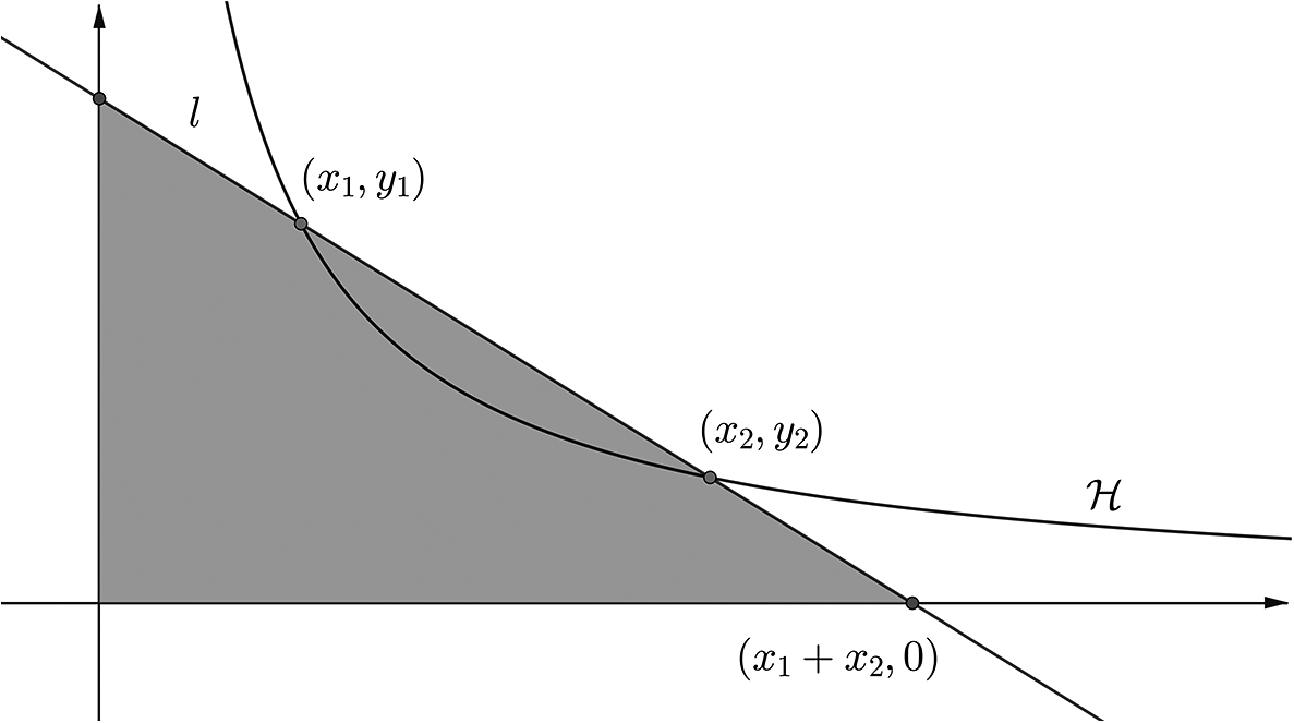
Lemma 4 Let l be the line through any two points $(x_1,y_1)$ and $(x_2,y_2)$ on $\mathcal {H}$ . Then, the line l intersects the x-axis at the point $(x_1+x_2,0)$ and the triangle determined by l and the coordinate axes has area precisely

(3.1) $$ \begin{align} \frac{1}{2} + \frac{(x_1-x_2)^2}{8 x_1 x_2}. \end{align} $$

In the limiting case, when the two points on $\mathcal {H}$ coincide, the line l becomes the tangent on $\mathcal {H}$ at $(x_1,y_1)$ and the above area is always equal to $1/2$ .

Proof Consult Figure 6. The equation of the line through $(x_1,y_1)$ and $(x_2,y_2)$ reads

$$\begin{align*}y - y_1 = \frac{y_2-y_1}{x_2-x_1} (x - x_1), \end{align*}$$

while $y_1=1/(4x_1)$ and $y_2=1/(4x_2)$ enable its simplification as

$$\begin{align*}y = \frac{-x+x_1+x_2}{4x_1 x_2}. \end{align*}$$

The two segments that l cuts off from the axes have lengths $x_1+x_2$ and $(x_1+x_2)/ (4x_1 x_2)$ , so the area of the triangle in question equals $(x_1+x_2)^2/(8x_1 x_2)$ , which easily transforms into (3.1).

Figure 6

Enclosed triangle.

A similar computation finds the equation of the tangent line on $\mathcal {H}$ at $(x_1,y_1)$ as

$$\begin{align*}y = \frac{-x+2x_1}{4x_1^2}, \end{align*}$$

so the segments cut off from the axes now have lengths $2x_1$ and $1/(2x_1)$ , while the formed triangle has area $1/2$ .

Now, we turn to the actual proof of the second theorem. Suppose that there is a convex polygon $\mathcal {P}$ with ${\text {area}}(\mathcal {P})\geqslant 1$ , all sides of length $a>0$ , and all vertices contained in the above set $\mathcal {S}$ . We will gradually narrow down several possibilities until we arrive at a final contradiction.

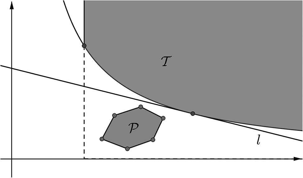
Let us first suppose that $\mathcal {P}$ is fully contained in the region $\mathcal {S}$ (see Figure 7). Then, $\mathcal {P}$ and $\mathcal {T}$ are disjoint convex sets, and they can be separated by a line, via an elementary version of the Hahn–Banach separation theorem. By moving the separation line upward until it touches $\mathcal {T}$ , and possibly rotating it counterclockwise if the touching point happens to be $(1,1/4)$ , we obtain a tangent l on $\mathcal {H}$ such that the polygon $\mathcal {P}$ lies below it. The area of $\mathcal {P}$ can then be bounded from above by the area of the triangle formed by l and the coordinate axes, so Lemma 4 gives ${\text {area}}(\mathcal {P})\leqslant 1/2$ , which is a contradiction.

Figure 7

Separating tangent.

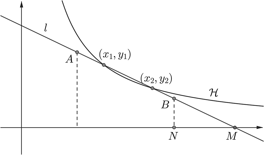
Thus, $\mathcal {T}$ actually intersects the polygon $\mathcal {P}$ , but it can intersect only one of its sides contained in the upper boundary of $\mathcal {P}$ , call it $\overline {AB}$ (see Figure 8). Otherwise, it would also contain some of the vertices of $\mathcal {P}$ , but we assumed that all of the vertices are in the region $\mathcal {S}$ . Let $(x_1,y_1)$ and $(x_2,y_2)$ , for $x_1\leqslant x_2$ , be the intersection points of $\mathcal {H}$ and the side $\overline {AB}$ , allowing the possibility that the two points coincide. Also, let l be the line through $(x_1,y_1)$ and $(x_2,y_2)$ , or the line tangent to $\mathcal {H}$ at $(x_1,y_1)=(x_2,y_2)$ . Observing that $\mathcal {P}$ is, by its convexity, again contained in the triangle formed by l and the coordinate axes, the formula (3.1) from Lemma 4 now yields

$$\begin{align*}{\text{area}}(\mathcal{P})\leqslant \frac{1}{2} + \frac{(x_1-x_2)^2}{8 x_1 x_2} \leqslant \frac{1}{2} + \frac{a^2}{8 x_1 x_2}. \end{align*}$$

We clearly arrive at the contradiction with ${\text {area}}(\mathcal {P})\geqslant 1$ again if

• • $a<2$ (as $x_2\geqslant x_1\geqslant 1$ ),

• • or $x_1\geqslant 7a/8$ (as then also $x_2\geqslant 7a/8$ ).

Figure 8

Upper boundary of $\mathcal {P}$ .

Thus, in the following, we additionally assume that $a\geqslant 2$ and $x_1<7a/8$ . Without loss of generality, A has a smaller x-coordinate than B. However, A is then contained in the rectangle $[1,7a/8]\times [0,1/4]$ , the diagonal of which is

$$\begin{align*}\sqrt{\Big(\frac{7a}{8}-1\Big)^2+\Big(\frac{1}{4}\Big)^2}<a, \end{align*}$$

and there is no room inside that rectangle for another side of the polygon $\mathcal {P}$ . Consequently, A is the leftmost vertex of $\mathcal {P}$ . Next, recall that all vertices of $\mathcal {P}$ except A and B lie below the line l. Let M be the intersection of l with the x-axis, and let N be the foot of the perpendicular from B onto the x-axis (see Figure 8 again). By another claim from Lemma 4, the coordinates of M are $(x_1+x_2,0)$ . The diameter of triangle $\triangle BNM$ is

$$\begin{align*}|BM| < {\text{dist}}\big( (x_2,y_2), (x_1+x_2,0) \big) \leqslant x_1 + \frac{1}{4} < \frac{7a}{8} + \frac{1}{4} \leqslant a, \end{align*}$$

which leaves no room inside $\triangle BNM$ for another side of $\mathcal {P}$ . Thus, B is the rightmost vertex of the polygon $\mathcal {P}$ .

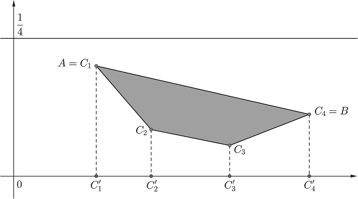
We can now denote the vertices of $\mathcal {P}$ counterclockwise as

$$\begin{align*}A= C_1,\, C_2,\, \ldots,\, C_{n-1},\, C_n=B, \end{align*}$$

knowing that $n\geqslant 3$ (see Figure 9). Let $C^{\prime }_i$ be the projection of $C_i$ onto the x-axis for $i=1,\ldots ,n$ . For every $1\leqslant i\leqslant n-1,$ we know that the projection of $\overline {C_i C_{i+1}}$ onto the y-axis has length at most $1/4$ , so the Pythagorean theorem and $a\geqslant 2$ give

$$\begin{align*}a^2 = |C_i C_{i+1}|^2 \leqslant |C^{\prime}_i C^{\prime}_{i+1}|^2 + \Big(\frac{1}{4}\Big)^2 \leqslant |C^{\prime}_i C^{\prime}_{i+1}|^2 + \frac{a^2}{64}, \end{align*}$$

which implies $|C^{\prime }_i C^{\prime }_{i+1}|\geqslant 7a/8$ . Ultimately,

$$\begin{align*}a = |AB| \geqslant |C^{\prime}_1 C^{\prime}_n| = \sum_{i=1}^{n-1} |C^{\prime}_i C^{\prime}_{i+1}| \geqslant \frac{7(n-1)a}{8}>a, \end{align*}$$

which leads to the ultimate contradiction and completes the proof of Theorem 2.

Figure 9

Estimating projections.