


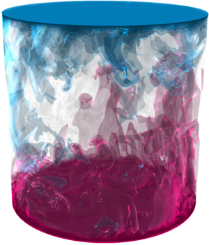





1. Introduction
Understanding thermally induced convection as it arises in the Earth's atmospheric/oceanic circulations and deducing its fundamental aspects from laboratory experiments is an ongoing endeavour which motivated numerous experimental and theoretical studies. In this realm, Rayleigh–Bénard convection (RBC), i.e. a fluid held between two parallel plates heated from below and cooled from above, is the most thoroughly investigated model system to study the complex physics behind natural convection such as pattern formation and the transition to turbulence (Bodenschatz, Pesch & Ahlers Reference Bodenschatz, Pesch and Ahlers2000; Ahlers, Grossmann & Lohse Reference Ahlers, Grossmann and Lohse2009b; Lohse & Xia Reference Lohse and Xia2010).
Most of the early theoretical advances were made by considering the system as infinitely extended in the lateral direction. For instance, conventional linear-stability analysis predicts the formation of two-dimensional rolls (Chandrasekhar Reference Chandrasekhar1961), while a weakly nonlinear analysis reveals the stability regimes of these rolls and their path to subsequent oscillatory- or stationary-type bifurcations (Schlüter, Lortz & Busse Reference Schlüter, Lortz and Busse1965; Busse Reference Busse1967, Reference Busse1978). In laboratory experiments, however, we must resort to laterally confined systems where our understanding is far less complete. In particular, when the lateral size of the container is close to or less than the height of the cell, the presence of sidewalls plays an important role (Roche Reference Roche2020; Shishkina Reference Shishkina2021). Therefore, this study focuses on the effects of different thermal sidewall boundary conditions on heat transfer and the emergence of different flow states.
Different sidewalls are known to affect the critical Rayleigh number  ${\textit {Ra}}_c$ above which convection sets in (Buell & Catton Reference Buell and Catton1983; Hébert et al. Reference Hébert, Hufschmid, Scheel and Ahlers2010), and perfectly conducting sidewalls have been found to delay the onset compared with adiabatic sidewalls. In an attempt to better understand the flow regimes above onset, bifurcation analyses were performed in a cubic domain for adiabatic (Puigjaner et al. Reference Puigjaner, Herrero, Giralt and Simó2004) and perfectly conducting sidewalls (Puigjaner et al. Reference Puigjaner, Herrero, Simó and Giralt2008). The bifurcation diagrams for the conducting sidewalls are generally more complex, and double-toroidal states predominate over the classical single-roll structure found for adiabatic sidewalls. Sidewalls also have a strong influence on pattern formation (Cross & Hohenberg Reference Cross and Hohenberg1993; de Bruyn et al. Reference de Bruyn, Bodenschatz, Morris, Trainoff, Hu, Cannell and Ahlers1996; Bodenschatz et al. Reference Bodenschatz, Pesch and Ahlers2000) and different sidewall boundary conditions lead to differences in observable patterns even in cells with large aspect ratio (Hu, Ecke & Ahlers Reference Hu, Ecke and Ahlers1993).
In RBC experiments, spurious sidewall heat fluxes are a major practical difficulty that can substantially bias global heat transport measurements. Ahlers (Reference Ahlers2000) reported that naive sidewall corrections can overstate Nusselt number measurements by up to  $20\,\%$ and underestimate the scaling of the Nusselt number
 ${\textit {Nu}}$ with respect to the Rayleigh number
 ${\textit {Ra}}$ (
 ${\textit {Nu}} \sim {\textit {Ra}}^{\lambda }$) reflected in the reduction of the scaling exponent
 $\lambda$ by approximately
 $2\,\%$, underscoring the importance of more sophisticated sidewall corrections. Roche et al. (Reference Roche, Castaing, Chabaud, Hébral and Sommeria2001) further emphasized this conclusion by showing that the sidewall corrections can be considerably larger than assumed, leading to scaling exponents closer to the turbulent scaling of
 ${\textit {Nu}} \sim {\textit {Ra}}^{1/3}$ (Grossmann & Lohse Reference Grossmann and Lohse2000, Reference Grossmann and Lohse2001, Reference Grossmann and Lohse2004) than previously measured. Probably the most important question in convection today is whether the ultimate regime in confined geometries has the same scaling as predicted for unbounded domains, i.e.
 ${\textit {Nu}} \sim {\textit {Ra}}^{1/2}$ (up to different logarithmic corrections), as proposed by Kraichnan (Reference Kraichnan1962) and Grossmann & Lohse (Reference Grossmann and Lohse2011). Another important question is when and how exactly the transition to the ultimate regime takes place in confined geometries. Laboratory experiments (Chavanne et al. Reference Chavanne, Chilla, Castaing, Hebral, Chabaud and Chaussy1997; Niemela et al. Reference Niemela, Skrbek, Sreenivasan and Donnely2000; Chavanne et al. Reference Chavanne, Chillà, Chabaud, Castaing and Hébral2001; Ahlers, Funfschilling & Bodenschatz Reference Ahlers, Funfschilling and Bodenschatz2009a; Ahlers et al. Reference Ahlers, He, Funfschilling and Bodenschatz2012; He et al. Reference He, Funfschilling, Nobach, Bodenschatz and Ahlers2012; Urban et al. Reference Urban, Hanzelka, Musilova, Kralik, Mantia, Srnka and Skrbek2014; Roche Reference Roche2020) in this extremely high
 ${\textit {Ra}}$ regime are notoriously difficult to perform and potentially sensitive to several unknowns of the system, one of which is the influence of imperfectly isolated/adiabatic sidewalls.
Numerical simulations were performed incorporating thermal conduction in the solid sidewall to clarify the differences between an ideal adiabatic set-up and a finite thermal conductivity sidewall (Verzicco Reference Verzicco2002; Stevens, Lohse & Verzicco Reference Stevens, Lohse and Verzicco2014; Wan et al. Reference Wan, Wei, Verzicco, Lohse, Ahlers and Stevens2019). The results of these studies suggest that different thermal properties of the sidewall alter the mean flow structure, leading to significant differences in global heat transport in the low to mid  ${\textit {Ra}}$ range. However, this effect vanishes for larger
 ${\textit {Ra}}$, at least when the sidewall temperature is constant and maintained at the arithmetic mean of upper and lower plate temperatures. Conversely, if the sidewall temperature deviates from the arithmetic mean, differences in heat transport persist even for large
 ${\textit {Ra}}$. This indicates that it is more important to keep the environment at the correct temperature than to shield the interior of the cell from its surroundings.
Despite extensive previous work, the spatial distribution of flow and heat transport in confined geometries with different thermal boundary conditions has not been exhausted, especially the conditions related to real experimental sidewall boundary conditions. In the present work, we investigate RBC with the following thermal sidewall boundary conditions: adiabatic, constant temperature (isothermal) and linear temperature. In the first part of the results, we focus on a steady-state analysis based on an adjoint descent algorithm (Farazmand Reference Farazmand2016) to identify different flow states, their properties and their evolution over  ${\textit {Ra}}$. In the second part, the analysis is complemented and extended to higher
 ${\textit {Ra}}$ into the turbulent regime by a set of direct numerical simulations (DNS) for a two-dimensional (2-D) box and 3-D cylindrical set-up, covering a range of
 $10^{3}\leqslant {\textit {Ra}}\leqslant 4\times 10^{10}$ and
 $10^{3}\leqslant {\textit {Ra}} \leqslant 10^{9}$, respectively, aiming for a more complete picture. We first present our numerical methods, discuss the results and conclude with our main findings.
2. Numerical methods
2.1. Governing equations
The dimensionless control parameters in RBC are the Rayleigh number  ${\textit {Ra}} \equiv \alpha g \Delta H^{3}/(\kappa \nu )$, the Prandtl number
 ${\textit {Pr}}\equiv \nu /\kappa$ and the width-to-height aspect ratio of the box,
 $\varGamma \equiv L/H$. Here,
 $\alpha$ denotes the isobaric thermal expansion coefficient,
 $\nu$ the kinematic viscosity,
 $\kappa$ the thermal diffusivity of the fluid,
 $g$ the acceleration due to gravity,
 $\varDelta \equiv T_+-T_-$ the difference between the temperatures at the lower (
 $T_+$) and upper (
 $T_-$) plates,
 $H$ the distance between the parallel plates (the container height) and
 $L$ the length of the container or the diameter in the case of a cylindrical set-up. In this study, we focus on variations with
 ${\textit {Ra}}$, while
 ${\textit {Pr}}=1$ is fixed for most results in this paper except for a
 ${\textit {Pr}}$-dependence study in § 4.5, and
 $\varGamma =1$ is held constant throughout the study.
The governing equations in the Oberbeck–Boussinesq approximation for the dimensionless, incompressible velocity  ${\boldsymbol {u}}$, temperature
 $\theta$ and kinematic pressure
 $p$ read as follows:
 \begin{equation} \left.\begin{gathered} \partial\boldsymbol{u}/\partial t+\boldsymbol{u}\boldsymbol{\cdot} {\boldsymbol{\nabla}} \boldsymbol{u}+{\boldsymbol{\nabla}} {p}= \sqrt{Pr/Ra} \nabla^{2} \boldsymbol{u}+ {\theta}{\boldsymbol{e}}_z , \\ \partial{\theta}/\partial t+\boldsymbol{u}\boldsymbol{\cdot} {\boldsymbol{\nabla}} {\theta}= 1/\sqrt{Pr Ra} \nabla^{2} {\theta}, \quad {\boldsymbol{\nabla}} \boldsymbol{\cdot} \boldsymbol{u} =0. \end{gathered}\right\}\end{equation}
The equations were made dimensionless using the free-fall velocity  $u_{ff}\equiv (\alpha g \Delta H)^{1/2}$, the free-fall time
 $t_{ff}\equiv H/u_{ff}$, the temperature difference
 $\varDelta \equiv T_+-T_-$ between bottom (
 $T_+$) and top (
 $T_-$) plates and
 $H$ the cell height. Here,
 ${\boldsymbol {e}}_z$ is the unit vector in the vertical
 $z$-direction. This set of equations is solved with the direct numerical solver goldfish, which uses a fourth-order finite volume discretization on a staggered grid and a third-order Runge–Kutta time scheme. The code has been widely used in previous studies and validated against other direct numerical simulation codes (Kooij et al. Reference Kooij, Botchev, Frederix, Geurts, Horn, Lohse, van der Poel, Shishkina, Stevens and Verzicco2018; Reiter et al. Reference Reiter, Shishkina, Lohse and Krug2021a).
2.2. Boundary conditions
We study 2-D RBC in a square box and 3-D RBC in a cylindrical domain. The set-ups and profiles of the sidewall boundary conditions (BCs) used are shown in figure 1. The adiabatic, linear and (almost) constant conditions for the sidewall region  $\delta V_S$ are defined by
 $$\begin{gather} \text{adiabatic:} \quad \partial \theta/\partial{\chi} = 0, \end{gather}$$
 $$\begin{gather}\text{linear:} \quad \theta = \theta_+\ {+}\ z \left(\theta_-\ {-}\ \theta_+ \right), \end{gather}$$
 $$\begin{gather}\text{constant:} \quad \theta = \begin{cases} \dfrac{-k(2z-1)}{k+2 z} \left(\theta_+\ {-}\ \theta_m \right), & 0 \leqslant z\leqslant 1/2,\\ \dfrac{k(2z-1)}{k-2z+2}\left(\theta_-\ {-}\ \theta_m \right), & 1/2 < z \leqslant 1, \end{cases} \end{gather}$$
with the temperature of the lower plate  $\theta _+=1/2$, the temperature of the upper plate
 $\theta _-=-1/2$, their arithmetic mean
 $\theta _m=0$,
 $z \equiv z/H \in [0,1]$ and
 $\chi =x$ for the box and
 $\chi =r$ for the cylinder, respectively. As for the constant temperature conditions, most of the sidewall is kept at a nearly uniform temperature (
 $\theta _m$), except for the transition regions in the vicinity of the top and bottom plates to ensure a smooth temperature distribution. The parameter
 $0< k\ll 1$ in (2.4) defines the thickness of the transition layer. Here, we used
 $k=0.01$, which gives a fairly sharp albeit sufficiently smooth transition, as can be seen in figure 1(c). Moreover, the velocity no-slip conditions apply to all walls, i.e.
 $\boldsymbol {u}|_{wall}= 0$.
Two-dimensional numerical set-up of (a) adiabatic, (b) linear and (c) constant sidewall temperature boundary conditions. (d) Sketch of cylindrical domain. Profiles next to (b,c) show the imposed sidewall temperature distribution.

2.3. Adjoint-descent method
A complementary analysis to DNS is the study of the Boussinesq equations by means of its invariant solutions. Hopf (Reference Hopf1948) conjectured that the solution of the Navier–Stokes equations can be understood as a finite but possibly large number of invariant solutions, and turbulence from this point of view is the migration from the neighbourhood of one solution to another. While highly chaotic systems seem too hopelessly complex to understand, laminar or weakly chaotic flows can often be captured quite well with this approach. In this work, we focus solely on solutions for steady states (equilibrium).
Determining steady-state solutions can be quite difficult, especially when the number of dimensions is large as it is the case for most fluid mechanical problems. The most commonly used numerical method for this task is Newton's method, which usually uses the generalized minimal residual (GMRES) algorithm to solve the corresponding systems of linear equations (Saad & Schultz Reference Saad and Schultz1986). This method generally shows fast convergence rates when the initial estimate is close to the equilibrium point. However, if the initial estimate is too far from the equilibrium, Newton's method often fails. In particular, for fluid mechanics, the basin of attraction of Newton's method can be quite small, making the search for steady states highly dependent on the initial guess. Here, we consider an alternative approach recently proposed by Farazmand (Reference Farazmand2016) based on an adjoint method. Farazmand (Reference Farazmand2016) has shown that this adjoint-descent method can significantly improve the chance of convergence compared with the Newton-descent method, and thus more reliably capture equilibrium states from a given initial state, but at the cost of a generally slower convergence rate. A detailed derivation of the algorithm can be found in Farazmand (Reference Farazmand2016). Below we sketch the idea of the method. Suppose we want to find equilibrium solutions of a particular PDE (in our case the Boussinesq equations)
 \begin{equation} \partial_t {\boldsymbol{u}} = F({\boldsymbol{u}}), \end{equation}
with  ${\boldsymbol {u}}={\boldsymbol {u}}(\boldsymbol {x}, t)$. The equilibriums of
 $F({\boldsymbol {u}})$ can be generally unstable and therefore difficult to detect. The idea is to search for a new partial differential equation (PDE), i.e.
 \begin{equation} \partial_\tau {\boldsymbol{u}} = G({\boldsymbol{u}}), \end{equation}
which solutions always converge to the equilibrium solutions of (2.5) when the fictitious time  $\tau$ goes to infinity
 \begin{equation} \|{F({\boldsymbol{u}})}\|_\mathcal{A}^{2} \rightarrow 0 \quad \text{as} \ \tau \rightarrow \infty, \end{equation}
with the weighted energy norm  $\|{{\cdot }}\|_\mathcal {A} \equiv \langle \cdot, \cdot \rangle _\mathcal {A} \equiv \langle \cdot, \mathcal {A} \cdot \rangle$ for a certain real self-adjoint and positive definite operator
 $\mathcal {A}$. The value of
 $F({\boldsymbol {u}})$ evolves along a trajectory
 ${\boldsymbol {u}}^{\prime }$ in accordance with
 \begin{equation} \tfrac{1}{2} \partial_\tau \|{F({\boldsymbol{u}})}\|_{\mathcal{A}}^{2} = \langle \delta F({\boldsymbol{u}}, {\boldsymbol{u}}^{\prime}), F({\boldsymbol{u}}) \rangle_{\mathcal{A}}, \end{equation}
where  $\delta F({\boldsymbol {u}},{\boldsymbol {u}}^{\prime }) \equiv \lim _{\varepsilon \to 0}\,({F({\boldsymbol {u}} + \varepsilon {\boldsymbol {u}}^{\prime })-F({\boldsymbol {u}})})/{\varepsilon }$ of
 $F({\boldsymbol {u}})$ is the functional Gateaux derivative at
 ${\boldsymbol {u}}$ in the direction
 ${\boldsymbol {u}}^{\prime }$. In the Newton-descent method, the search direction
 ${\boldsymbol {u}}^{\prime }$ is approximated from
 $\delta F({\boldsymbol {u}},{\boldsymbol {u}}^{\prime }) = - F({\boldsymbol {u}})$ by using, for example, a GMRES iterative algorithm. For the adjoint-descent method, on the other hand, we rewrite (2.8) in the form
 \begin{equation} \tfrac{1}{2} \partial_\tau \|{F({\boldsymbol{u}})}\|_\mathcal{A}^{2} = \langle {\boldsymbol{u}}^{\prime}, \delta F^{{{\dagger}}}({\boldsymbol{u}}, F({\boldsymbol{u}}))\rangle_\mathcal{A}, \end{equation}
where  $\delta F^{{\dagger} }$ is the adjoint operator of the functional derivative
 $\delta F$. For
 ${\boldsymbol {u}}^{\prime } = -\delta F^{{\dagger} }({\boldsymbol {u}}, F({\boldsymbol {u}}))$ one guarantees that
 $\|{F({\boldsymbol {u}})}\|_{\mathcal {A}}^{2}$ decays to zero along the trajectory
 ${\boldsymbol {u}}^{\prime }$, since then
 $\frac {1}{2} \partial _\tau \|{F({\boldsymbol {u}})}\|_{\mathcal {A}}^{2} = -\|{\delta F^{{\dagger} }({\boldsymbol {u}}, F({\boldsymbol {u}}))}\|_\mathcal {A}^{2}$. Letting
 ${\boldsymbol {u}}$ evolve along the adjoint search direction ensures the convergence to an equilibrium, thus we find the desired PDE
 $G({\boldsymbol {u}}) \equiv {\boldsymbol {u}}^{\prime }$, i.e.
 \begin{equation} G({\boldsymbol{u}}) ={-}\delta F^{{{\dagger}}}({\boldsymbol{u}}, F({\boldsymbol{u}})). \end{equation}
The choice of the norm  $\|{\cdot }\|_{\mathcal {A}}$ is important for the algorithm to be numerically stable and is explained in more detail in appendix. As mentioned, the operator
 $\mathcal {A}$ should be real-valued, positive definite and self-adjoint. Following Farazmand (Reference Farazmand2016), we use an operator
 $\mathcal {A}$ that is closely related to the inversed Laplacian, i.e.
 $\mathcal {A} = (\boldsymbol{\mathsf{I}} - \alpha \nabla ^{2})^{-1}$, where
 $\boldsymbol{\mathsf{I}}$ is the identity operator and
 $\alpha$ is a non-negative scalar parameter. For
 $\alpha =0$ this norm converges to the
 $L^{2}$-norm and for
 $\alpha >0$ it effectively dampens smaller scales and provides a better numerical stability.
The linear adjoint equations for the Boussinesq equations (2.1) read
 \begin{equation} \left.\begin{gathered}
-\partial_\tau{\boldsymbol{u}} =
\left({\boldsymbol{\nabla}}
\tilde{{\boldsymbol{u}}}^{\prime\prime} +
({\boldsymbol{\nabla}}
\tilde{{\boldsymbol{u}}}^{\prime\prime})^{\text{T}} \right)
{\boldsymbol{u}} -
\tilde{\theta}^{\prime\prime}{\boldsymbol{\nabla}}\theta -
{\boldsymbol{\nabla}} p^{\prime\prime} + \sqrt{Pr/Ra}
\nabla^{2} \tilde{{\boldsymbol{u}}}^{\prime\prime}, \\
-\partial_\tau\theta = {\boldsymbol{u}} \boldsymbol{\cdot}
{\boldsymbol{\nabla}} \tilde{\theta}^{\prime\prime} +
1/\sqrt{PrRa} \nabla^{2} \tilde{\theta}^{\prime\prime} +
{\boldsymbol{e}}_z\boldsymbol{\cdot}
\tilde{{\boldsymbol{u}}}^{\prime\prime},\\
{\boldsymbol{\nabla}} \boldsymbol{\cdot}
{\boldsymbol{u}}^{\prime\prime} =0, \quad
{\boldsymbol{\nabla}} \boldsymbol{\cdot} {\boldsymbol{u}}
=0; \end{gathered}\right\} \end{equation}
(see derivations in appendix). Here, the double prime fields  ${\boldsymbol {u}}^{\prime \prime }$ and
 $\theta ^{\prime \prime }$ denote the residuals of the Navier–Stokes equation (2.1), i.e.
 \begin{equation} \left.\begin{gathered} {\boldsymbol{u}}^{\prime\prime} \equiv{-}{\boldsymbol{u}} \boldsymbol{\cdot} {\boldsymbol{\nabla}} {\boldsymbol{u}} - {\boldsymbol{\nabla}} p + \sqrt{Pr/{\textit{Ra}}} \nabla^{2} {\boldsymbol{u}} + {\boldsymbol{e}}_z \theta, \\ \theta^{\prime\prime} \equiv{-}{\boldsymbol{u}} \boldsymbol{\cdot} {\boldsymbol{\nabla}} \theta + 1/\sqrt{Pr{\textit{Ra}}} \nabla^{2} \theta, \end{gathered}\right\} \end{equation}
and  $\tilde {{\boldsymbol {u}}}^{\prime \prime } \equiv \mathcal {A}\boldsymbol {{\boldsymbol {u}}}^{\prime \prime }$ as well as
 $\tilde {\theta }^{\prime \prime } \equiv \mathcal {A}\boldsymbol {\theta }^{\prime \prime }$. For simplicity, let
 $\boldsymbol {q} \equiv ({\boldsymbol {u}}, \theta )$, then the adjoint-descent method consists of three steps
(i) Find the residuals
 $\boldsymbol {q}^{\prime \prime }$ according to (2.12).
(ii) Solve
$\tilde {\boldsymbol {q}}^{\prime \prime } = \mathcal {A}\boldsymbol {q}^{\prime \prime }$ for $\tilde {\boldsymbol {q}}^{\prime \prime }$.(iii) Update
$\boldsymbol {q}$ according to (2.11).


In step (i), we solve the time stepping (2.1), where we use a standard pressure projection method and treat the diffusion term implicitly. The time step size  $\Delta t$ can be chosen independently of the artificial time step size
 $\Delta \tau$ of the adjoint equations. For step (ii), using the energy norm
 $\|{\cdot }\|_{\mathcal {A}}$ with the operator
 $\mathcal {A} = (\boldsymbol{\mathsf{I}} - \alpha \nabla ^{2})^{-1}$, we solve the Helmholtz-type equation
 $(\boldsymbol{\mathsf{I}} - \alpha \nabla ^{2})\tilde {\boldsymbol {q}}^{\prime \prime } = \boldsymbol {q}^{\prime \prime }$. The integration of the adjoint equations in step (iii) is similar to step (i), but all terms are treated explicitly. Through tests, we found that the artificial time step
 $\Delta \tau$ can be chosen much larger than
 $\Delta t$ in some cases, i.e. for large
 ${\textit {Ra}}$.
The BCs of  $\tilde {{\boldsymbol {u}}}^{\prime \prime }$ and
 $\tilde {\theta }^{\prime \prime }$ result from integration by parts in the derivation of the adjoint equations. Evaluation of the adjoint operator of the diffusion terms yields
 \begin{equation} \int_V \tilde{{\boldsymbol{u}}}^{\prime\prime} \nabla^{2} {\boldsymbol{u}}^{\prime} \,{\rm d}V = \int_V {\boldsymbol{u}}^{\prime} \nabla^{2} \tilde{{\boldsymbol{u}}}^{\prime\prime} \,{\rm d}V + \int_S {\boldsymbol{u}}^{\prime}({\boldsymbol{\nabla}}\tilde{{\boldsymbol{u}}}^{\prime\prime} \boldsymbol{\cdot} \boldsymbol{n})\,{\rm d}S - \int_S \tilde{{\boldsymbol{u}}}^{\prime\prime}({\boldsymbol{\nabla}}{\boldsymbol{u}}^{\prime} \boldsymbol{\cdot} \boldsymbol{n})\,{\rm d}S, \end{equation}
where we see the occurrence of two additional boundary terms (the last two terms) evaluated on the boundary domain  $S$. The first boundary term vanishes since the search direction
 ${\boldsymbol {u}}^{\prime }$ is zero on the boundaries. The second term can be eliminated if we also choose homogeneous Dirichlet BCs for the adjoint field
 $\tilde {{\boldsymbol {u}}}^{\prime \prime }$ on
 $S$. The same logic applies to homogeneous Neumann conditions. For the pressure field
 $p^{\prime \prime }$, we apply Neumann BCs on all walls. In this study, all flow states showed good overall convergence (
 $\|{F({\boldsymbol {u}})}\|_\mathcal {A}^{2}\leqslant 10^{-7}$) and the velocity fields where almost divergence free (
 $\|{\boldsymbol {\nabla }\boldsymbol {\cdot }{{\boldsymbol {u}}}}\|_{L^{2}}\leqslant 10^{-5}$). However, the rigorous verification of the chosen pressure BCs has yet to be performed. Another interesting point, reserved for later investigation, is whether a vorticity–streamfunction formulation might be better suited to resolve issues with the BCs.
For the steady-state analysis, we use a Galerkin method with Chebyshev bases in  $x$ and
 $z$ directions and a quasi-inverse matrix diagonalization strategy for better efficiency (Shen Reference Shen1995; Julien & Watson Reference Julien and Watson2009; Mortensen Reference Mortensen2018; Oh Reference Oh2019). The code is publicly available (Reiter Reference Reiter2021). We use an implicit backward Euler time discretization and alias the fields using the
 $2/3$ rule by setting the last
 $1/3$ high-frequency spectral coefficients to zero after evaluating the nonlinear terms. When used as a direct numerical solver, we found excellent agreement with our finite-volume code goldfish. In addition, the steady states from the adjoint-descent method showed excellent agreement with those found by an alternative Newton-GMRES iteration. Figure 2 shows the convergence rates for three different
 ${\textit {Ra}}$, starting from the same initial state. Overall, we find that the convergence chance is improved over the Newton-descent method, although the convergence rate suffers and larger
 ${\textit {Ra}}$ are either not feasible with the current approach as implemented in our code or diverge after some time. Therefore, we restrict the steady-state analysis to flows in the range
 ${\textit {Ra}}\leqslant 10^{7}$ and investigate larger
 ${\textit {Ra}}$ using DNS. One conceivable problem with the current approach is that the currently used energy norm with the operator
 $\mathcal {A}\equiv (\boldsymbol{\mathsf{I}} - \alpha \nabla ^{2})^{-1}$ dampens smaller scales in order to increase the stability of the algorithm. But for larger
 ${\textit {Ra}}$, smaller scales become important to resolving the boundary layers sufficiently, so the algorithm is likely to take longer to converge or the damping of the smaller scales will be too severe to reach convergence overall. Using smaller values of
 $\alpha$ could lead to better results in that case, as this emphasizes smaller scales more. Preliminary analyses suggest that in some cases smaller
 $\alpha$ leads to a better chance of convergence. In the future, the convergence rate might be improved by employing a hybrid adjoint-descent and Newton-GMRES approach, as proposed by Farazmand (Reference Farazmand2016). Alternative gradient optimization techniques are also conceivable to boost convergence speed.
Convergence of the adjoint-descent method for three different  ${\textit {Ra}}$, starting from the same initial field. The time-step size for which the algorithm is just stable increases with
 ${\textit {Ra}}$, i.e. for these cases we used
 $\Delta \tau = 0.05$ (
 ${\textit {Ra}}=10^{4}$),
 $\Delta \tau = 0.2$ (
 ${\textit {Ra}}=10^{5}$) and
 $\Delta \tau = 0.7$ (
 ${\textit {Ra}}=10^{6}$). All three cases converged to large-scale circulation flow states as described in § 3.2.

3. Steady-state analysis
In this section, we study steady states in 2-D RBC for  ${\textit {Ra}}\leqslant 10^{7}$. In what follows, we refer to flow states as single or multiple solutions connected by inherent symmetries of the system. For example, the single-roll state (SRS) in two dimensions can exist in two forms, either circulating clockwise or counterclockwise, but is considered as a single flow state that is invariant under reflection. Steady-state solutions of the SRS state have been investigated in laterally periodic flows with stress-free velocity BCs on the horizontal walls (Wen et al. Reference Wen, Chini, Kerswell and Doering2015, Reference Wen, Goluskin, LeDuc, Chini and Doering2020b) and with no-slip BCs (Sondak, Smith & Waleffe Reference Sondak, Smith and Waleffe2015; Waleffe, Boonkasame & Smith Reference Waleffe, Boonkasame and Smith2015; Wen, Goluskin & Doering Reference Wen, Goluskin and Doering2020a; Kooloth, Sondak & Smith Reference Kooloth, Sondak and Smith2021). Bifurcations and different flow states have already been studied in laterally unbounded RBC (Zienicke, Seehafer & Feudel Reference Zienicke, Seehafer and Feudel1998), in laterally bounded RBC for a cubic domain (Puigjaner et al. Reference Puigjaner, Herrero, Simó and Giralt2008) and a 2-D square domain (Venturi, Wan & Karniadakis Reference Venturi, Wan and Karniadakis2010). Here, we focus on the onset of convection, the SRS and a vertically stacked double-roll state (DRS) in 2-D RBC for three different sidewall BCs as shown in figure 1.
3.1. Onset of convection
In RBC, there is a critical Rayleigh number  ${\textit {Ra}}_c$ above which the system bifurcates from the conduction state to coherent rolls. We calculate
 ${\textit {Ra}}_c$ using a linear stability analysis described in more detail in Reiter et al. (Reference Reiter, Zhang, Stepanov and Shishkina2021b). For adiabatic or linear (conductive) sidewall BCs, the conduction or base state is characterized by a linear temperature profile in the vertical direction with zero velocity field and independence from control parameters. However, for a constant temperature sidewall distribution, there is always a weak flow due to the horizontal temperature gradients, which resembles a four-roll state. In this case, we perform a steady-state search before analysing the local stability around this equilibrium point.
Figure 3 shows the linear growth rates of the four most unstable modes, which resemble the first four Fourier modes as depicted in the same figure. All three BCs initially bifurcate from the conduction state to a SRS. Adiabatic sidewalls lead to a lower critical Rayleigh number compared with isothermal sidewalls, which is to be expected (Buell & Catton Reference Buell and Catton1983; Shishkina Reference Shishkina2021). The onset for the adiabatic sidewall occurs at  ${\textit {Ra}}_c \approx 2.7 \times 10^{3}$ which agrees well within our resolution limit with Venturi et al. (Reference Venturi, Wan and Karniadakis2010), who report a critical
 ${\textit {Ra}}$ of approximately
 $2582$. The onset for the linear sidewall occurs at
 $5.1\times 10^{3}$ and the onset for the constant sidewall occurs slightly later at
 $5.6\times 10^{3}$. This indicates that the interaction of the convective field – as present for the constant sidewall BC – with the unstable modes is weak and its influence on the onset is small.
Growth rates  $\sigma$ as determined from linear-stability analysis for the four most unstable modes at the onset of convection in the 2-D cell for (a) adiabatic, (b) linear and (c) constant sidewall BCs. Each line represents a different unstable mode: single roll (black), vertically stacked double roll (red), horizontally stacked double-roll (grey) and four-roll (blue).

3.2. Single roll (states $\mathcal {S}_A^{1}$, $\mathcal {S}_L^{1}$, $\mathcal {S}_C^{1}$)


The SRS is arguably the most important state in RBC for aspect ratios around unity. It is the first mode to appear above the conduction state, as we have just seen, and prevails even up to largest  ${\textit {Ra}}$ in the form of large-scale circulation (LSC) on turbulent superstructures (Zhu et al. Reference Zhu, Mathai, Stevens, Verzicco and Lohse2018; Reiter et al. Reference Reiter, Shishkina, Lohse and Krug2021a). The SRS is stable and time independent for small
 ${\textit {Ra}}$ but oscillatory, chaotic or even completely vanishing for larger
 ${\textit {Ra}}$, as we will show in § 4.3. Here, we analyse its properties before collapse and show that the growth of secondary corner rolls plays an important role in its destabilization and that this process can be both suppressed and enhanced by different sidewall BCs.
Figure 4 shows the temperature and velocity fields of the SRS for different sidewall BCs. For all three BCs we can identify a large primary roll circulating counterclockwise and two secondary corner rolls. The corner rolls are most pronounced for the linear sidewall BC and the primary roll is nearly elliptical. The dimensionless heat flux is expressed in form of the Nusselt number  ${\textit {Nu}}\equiv \sqrt {{\textit {Ra}}{\textit {Pr}}} F_f H / \varDelta$ with the heat flux
 $F_f$ entering the fluid and the imposed temperature difference
 $\varDelta$;
 $F_f$ can be defined in different ways, especially in the presence of sidewall heat fluxes. Averaging the temperature equation in (2.1) over time, one obtains
 \begin{equation} \boldsymbol{\nabla}\boldsymbol{\cdot} \boldsymbol{F}=0, \quad \boldsymbol{F}\equiv {\boldsymbol{u}} \theta -1/\sqrt{{\textit{Ra}}{\textit{Pr}}} {\boldsymbol{\nabla}}{\theta}, \end{equation}
from which it follows that the total heat flux must vanish through the boundaries  $S=\delta V$, i.e.
 $\int _S (F\boldsymbol {\cdot } \boldsymbol {n}) \,\textrm {d}S = 0$. (However, local temperature fluxes through the sidewall can and do exist, as we discuss in § 4.2.) For isothermal sidewall BCs, asymmetric flow states with net non-zero sidewall heat fluxes are possible; in this case, the heat fluxes through the bottom and top plates would deviate from each other. However, in the present study, we found that all sidewall heat fluxes are approximately equal to zero when integrated vertically and the temperature gradient at the bottom plate is approximately equal to the temperature gradient at the top plate. Therefore, we define
 ${\textit {Nu}}$ based on the lower (hot) plate at
 $z=0$
 \begin{equation} {\textit{Nu}} \equiv{-}\frac{1}{A_+}\int_{S_+} \frac{\partial \theta}{\partial z} {\rm d}{S_+}, \end{equation}
with the bottom plate domain  $S_+$ and its surface area
 $A_+$. The dimensionless momentum transport is given by the Reynolds number
 \begin{equation} Re \equiv \sqrt{{\textit{Ra}}/{\textit{Pr}}} \sqrt{\langle \boldsymbol{U}^{2}\rangle_V} L , \end{equation}
based on total kinetic energy of the mean field velocity  $\boldsymbol {U}$. Here,
 $\langle \cdot \rangle _V$ denotes a volume average.
SRS for (a) adiabatic ( ${\textit {Ra}}=10^{6}$), (b) linear (
 ${\textit {Ra}}=9\times 10^{4}$) and (c) constant (
 ${\textit {Ra}}=10^{6}$) sidewall temperature boundary conditions. Contours (streamlines) represent the temperature (velocity) field.

In the laminar regime, where the dissipation of the velocity and temperature field is determined by the contributions of the boundary layers, we expect the total heat and momentum scaling  ${\textit {Nu}} \sim {\textit {Ra}}^{1/4}$ and
 $Re \sim {\textit {Ra}}^{1/2}$ (Grossmann & Lohse Reference Grossmann and Lohse2000), respectively. Figure 5 shows that the former scaling shows up only for a very limited
 ${\textit {Ra}}$ range and only for the adiabatic boundary conditions. The SRS of the linear sidewall BCs is stable only up to
 ${\textit {Ra}}\leqslant 10^{5}$, then the corner rolls become strong enough to lead to a collapse of the SRS. The stability region where the steady states converge is too small to observe an unperturbed scaling. On the other hand, for the constant sidewall BCs, corner roll growth is less dominant. In this case, the reason why
 ${\textit {Nu}}$ scaling deviates from
 $1/4$, is that heat entering through the bottom/top can immediately escape through the sidewalls in the form of a ‘short circuit’, which dominates the lower
 ${\textit {Ra}}$ regime and is the reason why
 ${\textit {Nu}}$ is relatively large for small
 ${\textit {Ra}}$. For the adiabatic sidewall BC, we observe
 ${\textit {Nu}} \sim {\textit {Ra}}^{0.25}$ for
 $10^{4}\leqslant {\textit {Ra}} \leqslant 3\times 10^{5}$, followed by
 ${\textit {Nu}} \sim {\textit {Ra}}^{0.16}$ for
 $3\times 10^{5}\leqslant {\textit {Ra}}\leqslant 10^{6}$. Similarly, the growth of the corner rolls disturbs the convection wind, and
 ${\textit {Nu}}$ deviates from the ideal
 $1/4$ scaling. Looking at the
 $Re$ vs
 ${\textit {Ra}}$ scaling in figure 6, we find the theoretically predicted scaling of
 $1/2$ is better represented in comparison and the different sidewall BCs deviate less among themselves. This suggests that momentum transport is less affected by changing sidewall boundary conditions than heat transport.
Nusselt number  ${\textit {Nu}}$ for the SRSs for (a) adiabatic, (b) linear and (c) constant sidewall temperature boundary conditions. Plotted is the range where steady-state convergence is achieved. Further comparison of the steady-state analysis with the DNS results is shown in figure 18.

Reynolds number  $Re$ for the SRSs
 $\mathcal {S}_A^{1}$,
 $\mathcal {S}_L^{1}$,
 $\mathcal {S}_C^{1}$; (a) adiabatic, (b) linear and (c) constant sidewall temperature BCs. Plotted is the range where steady-state convergence is achieved.

3.2.1. Growth of corner rolls
The SRS is stable up to a certain  ${\textit {Ra}}$ limit. Above this limit, it may fluctuate, reverse orientation or even disappear altogether. This process occurs at
 ${\textit {Ra}}\approx 10^{6}$ for the adiabatic and constant temperature sidewall BCs and at
 ${\textit {Ra}}\approx 10^{5}$ for the linear sidewall BC. While up to this event the dynamic behaviour of the three different sidewall BCs is qualitatively very similar, from there on it differs. The constant sidewall BC case shows a time dependence, but remains in the SRS state without changing its orientation. The adiabatic and linear sidewall BCs, on the other hand, enter a more chaotic regime of regular and chaotic flow reversals (Xi & Xia Reference Xi and Xia2007; Sugiyama et al. Reference Sugiyama, Ni, Stevens, Chan, Zhou, Xi, Sun, Grossmann, Xia and Lohse2010), some of which are discussed in § 3.3. Of greatest importance here appears to be the presence and magnification of secondary corner rolls.
Figure 7(a) shows the vorticity field and streamfunction contour of 2-D RBC with adiabatic sidewalls at  ${\textit {Ra}}=7\times 10^{5}$. The existence of two corner vortices is apparent. Here, we define the corner roll size
 $\delta _{CR}$ based on the zero crossing, or stagnation point, of the vorticity
 $\omega \equiv \partial _x u_z - \partial _z u_x$ at the top plate, cf. Shishkina, Wagner & Horn (Reference Shishkina, Wagner and Horn2014). To understand the processes involved in the formation of the corner rolls, we write down the evolution equation for vorticity
 \begin{equation} \partial_t \omega = \underbrace{- {\boldsymbol{u}} \boldsymbol{\cdot} {\boldsymbol{\nabla}} \omega}_{\text{convection}} + \underbrace{\sqrt{Pr/Ra} \nabla^{2} \omega}_{\text{diffusion}} + \underbrace{\partial_x \theta}_{ \text{buoyancy}}. \end{equation}
It is evident that for steady states ( $\partial _t \omega = 0$) there must be an equilibrium between convection, diffusion and buoyancy forces. The three corresponding fields are shown in figure 7(b–d) zoomed in on the corner roll region. For this particular
 ${\textit {Ra}}$, all three contributions appear to be significant. We evaluate the size of the corner rolls (figure 8) and analyse contributions of diffusion, buoyancy and convection for all
 ${\textit {Ra}}$ (figure 7). For this purpose, we evaluate the absolute values of the volume averages for each term in the corner roll region, e.g.
 $\langle \vert \partial _x \theta \vert \rangle _{S_{CR}}$ represents the strength of the buoyancy term in the corner roll area
 $S_{CR}$, as shown in figure 7(c). The constant BC yields a notable exception because multiple corner rolls can exist. This can be sensed from figure 4(c). For small
 ${\textit {Ra}}$, the corner roll are dominant in the lower right and upper left corners, where the LSC detaches (ejects). For the other two BCs, these rolls are not present. Looking at (3.4), we realize that the presence of a horizontal temperature gradient can lead to the formation of vortex structures. This condition is present for the constant BCs, e.g. in the lower right corner, where the hot LSC detaches while the temperature is kept constant at zero, resulting in a (strong) negative temperature gradient. The two more ‘classical’ corner rolls first appear at larger
 ${\textit {Ra}}$, but soon take over in size, as can be seen in figure 8.
(a) Steady-state vorticity field and velocity streamlines for  ${\textit {Ra}}=7\times 10^{5}$ and adiabatic sidewalls. The corner roll size
 $\delta _{CR}$ is defined as the distance from the corner to the closest stagnation point at the plate. Bottom figures show the vorticity balance contributions according to (3.4) in the corner roll domain, i.e. (b) diffusion, (c) buoyancy and (d) convection. The same contour levers were used for (b–d).

Growth of the corner roll size  $\delta _{CR}$ for (a) adiabatic, (b) linear and (c) constant sidewall temperature BCs. Adiabatic BC shows two distinct regions, a buoyancy-dominated regime and a regime where convective influx leads to a more rapid increase. For the constant BC, the corner rolls appear first in the plume ejecting corner (bottom right and upper left in figure 4) which is represented by the open symbols in (c), and only for larger
 ${\textit {Ra}}$ do they appear in the plume impacting region (closed symbols). Plotted is the range, where steady-state convergence is achieved.

The adiabatic and linear sidewall BCs each yield only two corner rolls. These are present from the onset of convection and grow until the collapse of the SRS (figure 8). The main difference between the two is that for the adiabatic sidewall, the corner rolls initially grow monotonically with respect to  ${\textit {Ra}}$, whereas for the linear sidewall BCs, the corner rolls are already quite large as soon as the SRS is present. Moreover, they also grow faster with respect to
 ${\textit {Ra}}$ (
 $\delta _{CR}\sim {\textit {Ra}}^{0.3}$) and soon cover almost
 $40\,\%$ of the width of the cell. Their large initial size combined with faster growth is the reason for premature SRS instability in linear sidewall BCs. Figure 9(b) shows that vorticity formation for the entire
 ${\textit {Ra}}$ range is mainly governed by buoyancy and balanced by diffusion. We assume the hot plumes carry warm fluid to the upper plate where it meets a cold sidewall, generating strong lateral gradients in the upper right corner and consequently vorticity, according to (3.4).
Strength of the vorticity balance contributions diffusion (black circles), buoyancy (yellow diamonds) and convection (green squares) in the corner roll region, according to (3.4). (a) Adiabatic, (b) linear and (c) constant sidewall temperature boundary conditions. Adiabatic BC shows two distinct regions, a buoyancy dominated regime and a regime where convective influx leads to a more rapid increase. For the constant BC, the corner rolls appear first in the plume ejecting corner (bottom right and upper left in figure 4) which is represented by the open symbols in (c), and only for larger  ${\textit {Ra}}$ do they appear in the plume impacting region (closed symbols). Plotted is the range, where steady-state convergence is achieved.

In the adiabatic case, on the other hand, the sidewall is warmer close to the corner, which leads to less vorticity generation by lateral temperature gradients and therefore smaller corner rolls. In the low  ${\textit {Ra}}$ regime, the corner rolls of the adiabatic sidewall are also governed by buoyancy, with a growth of the corner rolls of
 $\delta _{CR}\sim {\textit {Ra}}^{0.21}$ (figure 8a). This can be understood by dimensional arguments. Assuming convection can be neglected in (3.4), which is justified from the results in figure 9(a), we thus obtain
 $\sqrt {{\textit {Pr}}/{\textit {Ra}}} \nabla ^{2} \omega = \partial _x \theta$, or, in terms of a characteristic temperature
 $\theta _{CR}$ and a characteristic vorticity
 $\varOmega _{CR}$, we have
 $\nu ({\varOmega _{CR}}/{\delta _{CR}^{2}}) \sim {\theta _{CR}}/{\delta _{CR}}$, and thus
 \begin{equation} \delta_{CR} \sim \sqrt{\frac{Pr}{Ra}} \frac{\varOmega_{CR}}{\theta_{CR}}. \end{equation}
The evaluation (not shown here) of the characteristic vorticity in the corner roll regions by means of their root mean square value unveiled  $\varOmega \sim {\textit {Ra}}^{0.7}$. Assuming further that the temperature
 $\theta _{CR}$ is approximately constant over
 ${\textit {Ra}}$, we obtain
 $\delta _{CR}\sim {\textit {Ra}}^{0.20}$, which agrees remarkably well with
 $\delta _{CR}\sim {\textit {Ra}}^{0.21}$. Figure 8(a) discloses a transition at
 ${\textit {Ra}} \approx 3 \times 10^{5}$, above which the corner roll growth accelerates, exhibiting a scaling of
 $\delta _{CR}\sim {\textit {Ra}}^{0.49}$. Figure 9(a) indicates that convective processes begin to affect vorticity generation. Figure 7(d) reveals a region with strong convective vorticity current with the same sign as the buoyancy forces, which enhances the vorticity generation in this region (figure 7c). We interpret this as meaning that, above a certain
 ${\textit {Ra}}$, the primary roll of the SRS begins to feed the corner rolls until they become strong enough, eventually leading to the collapse of the SRS itself. We would like to note that the current analysis describes steady states up to
 ${\textit {Ra}}\leqslant 10^{6}$. An opposite trend was observed for larger
 ${\textit {Ra}}$ by Zhou & Chen (Reference Zhou and Chen2018), who found a slow shrinkage of the corner rolls that scales approximately with
 $\sim {\textit {Ra}}^{-0.085}$. It would be interesting to consolidate these results in future studies.
3.3. Double roll ($\mathcal {S}_A^{2}$, $\mathcal {S}_L^{2}$)


Having discussed the properties of the SRS state, we proceed to the DRS, as shown in figure 10. It consists of two vertically stacked hot and cold circulation cells rotating in opposite directions with an almost discrete temperature jump in the mid plane. The DRS was not identified as an equilibrium for the constant sidewall BCs, so we will discuss it exclusively for the adiabatic and linear sidewall set-ups. The DRS can coexist with the SRS, but is generally found at larger  ${\textit {Ra}}$. Here, we have tracked it in the range
 $10^{5} \leqslant {\textit {Ra}} < 7\times 10^{6}$ for adiabatic and
 $10^{5} \leqslant {\textit {Ra}} < 4\times 10^{6}$ for linear sidewall BCs. This range is consistent with Goldhirsch, Pelz & Orszag (Reference Goldhirsch, Pelz and Orszag1989) who described a roll-upon-roll state in 2-D RBC for
 ${\textit {Pr}}=0.71$ at
 ${\textit {Ra}}\approx 10^{5}$, but interestingly it was not found for
 ${\textit {Pr}}=6.8$.
DRS for (a) adiabatic and (b) linear. Contours (streamlines) represent the temperature (velocity) field.

From figure 11 we see that  ${\textit {Nu}}$ scales close to
 ${\textit {Nu}}\sim {\textit {Ra}}^{1/4}$, which corresponds to laminar scaling for RBC flows governed by boundary layer dissipation. Compared with the SRS, it is less effective in transporting heat from wall to wall, as evidenced by an overall smaller
 ${\textit {Nu}}$. This is actually to be anticipated, since one roll of the DRS can be conceptually viewed as a half-height, half-temperature gradient RBC system, implying a
 $16$ times smaller effective
 ${\textit {Ra}}$. However, this factor most likely overestimates the difference, since the mid plane velocity is much closer to a free-slip flow than a no-slip flow and the aspect ratio is two rather than one. In reality, a DRS has approximately the same
 ${\textit {Nu}}$ as a SRS with a
 $6$ times smaller
 ${\textit {Ra}}$.
Nusselt number  ${\textit {Nu}}$ for DRSs
 $\mathcal {S}_A^{2}$ and
 $\mathcal {S}_L^{2}$. (a) Adiabatic and (b) linear sidewall temperature BCs. Plotted is the range where steady-state convergence is achieved. Further comparison of the steady-state analysis with the DNS results is shown in figure 18.

The DRS is found to be time independent (stable) only for the adiabatic sidewall BCs for  ${\textit {Ra}}\leqslant 4 \times 10^{5}$. For other
 ${\textit {Ra}}$ it is either periodically oscillating or chaotic. In figure 12 we show characteristic frequencies of the DRS obtained by initializing DNS simulation with the steady-state solutions and evaluating the frequency spectra of
 ${\textit {Nu}}(t)$. The frequency is presented in free-fall time units. The DRS oscillates with a frequency of approximately
 $0.1$ for
 ${\textit {Ra}}\leqslant 10^{6}$ for both the adiabatic and linear set-ups, i.e. approximately one cycle every
 $10$ time units. This cycle corresponds to approximately half the circulation time of a cell, i.e. the characteristic velocity of the circulation is approximately
 $0.09 \sim 0.11$ and its size is
 $\approx 2 L$. Thus, the DRS oscillation frequency seems to be initially tied to the circulation time. When
 ${\textit {Ra}}$ exceeds
 $10^{6}$, we see the emergence of a more chaotic behaviour. Despite increasing turbulence, the DRS state persists and does not show transition to a SRS state for
 ${\textit {Ra}}<10^{7}$. In § 4.3 we will see that for larger
 ${\textit {Ra}}$ the DRS state is eventually replaced by a single-roll LSC again.
Maximum peak frequency  $f_{{max}}$ and average frequency
 $\bar {f}$ determined from
 ${\textit {Nu}}(t)$ for DRSs
 $\mathcal {S}_A^{2}$ and
 $\mathcal {S}_L^{2}$ for (a) adiabatic and (b) linear sidewall temperature BCs. Plotted is the range where steady-state convergence is achieved.

The DRS state is not merely an equilibrium solution, but more fundamentally there is a regime in  ${\textit {Ra}}$ where the DRS is the preferred flow state to which all initial states tested in this work tend towards. Starting from random perturbations, one usually first finds a SRS, which soon goes through a series of flow reversals and restabilizations until it evolves to the DRS state. This process is depicted in an SRS–DRS phase space picture in figure 13. The horizontal axis represents the SRS, and the vertical axis represents the DRS. This process is qualitatively the same for adiabatic and linear sidewall boundary conditions. We do not address the flow reversal process, as it is described in more detail in Xi & Xia (Reference Xi and Xia2007), Sugiyama et al. (Reference Sugiyama, Ni, Stevens, Chan, Zhou, Xi, Sun, Grossmann, Xia and Lohse2010), Castillo-Castellanos, Sergent & Rossi (Reference Castillo-Castellanos, Sergent and Rossi2016) and Zhao, Cai & Jiang (Reference Zhao, Cai and Jiang2019), but note that the intermediate flow fields bear striking resemblance to the proper orthogonal decomposition modes presented in Podvin & Sergent (Reference Podvin and Sergent2015, Reference Podvin and Sergent2017). We want to stress that the transition time is surprisingly long. It can take up to several thousand free-fall time units for the flow to settle in the DRS state, so it can be missed if the observation window is too small.
Phase space trajectories from a single roll ( $\mathcal {S}_A^{1}$/
 $\mathcal {S}_L^{1}$) to a DRS (
 $\mathcal {S}_A^{2}$/
 $\mathcal {S}_L^{2}$) for (a) adiabatic sidewall at
 ${\textit {Ra}}=2\times 10^{6}$ and (b) linear sidewall BCs at
 ${\textit {Ra}}=1.5\times 10^{5}$.

4. Direct numerical simulations
In addition to the steady-state analysis, we performed a series of DNS of RBC for two dimensions in a square and three dimensions in a cylinder with  $\varGamma =1$ and
 ${\textit {Pr}}=1$, covering
 ${\textit {Ra}}$ from the onset of convection to
 $4.64 \times 10^{10}$ and
 $10^{9}$, respectively. The highest
 ${\textit {Ra}}$ in two dimensions was simulated on a
 $1024^{2}$ grid with at least
 $15$ grid points in the thermal boundary layer and performed for several thousand free-fall time units, ensuring adequate spatial resolution and temporal convergence. The largest simulation for the cylindrical set-up was performed on a
 $N_r \times N_\varphi \times N_z = 128 \times 256 \times 320$ grid, with approximately
 $10$ points inside the thermal and viscous boundary layers and the averaging statistics were collected for at least
 $600$ free-fall time units.
4.1. Vertical temperature profiles
Figure 14 shows the horizontally averaged temperature profiles  $\langle \theta \rangle _A$ for all of the conducted simulations. We first remark the similarity between two and three dimensions. For example, both show the feature of a weakly stabilizing positive temperature gradient in the mid plane for small
 ${\textit {Ra}}$ and adiabatic BCs (figure 14a,d). This phenomenon is often found in the interior of the bulk (Tilgner, Belmonte & Libchaber Reference Tilgner, Belmonte and Libchaber1993; Brown & Ahlers Reference Brown and Ahlers2007; Wan et al. Reference Wan, Wei, Verzicco, Lohse, Ahlers and Stevens2019) and is caused by the thermal signature of the LSC. As the thermal plume of the LSC climbs up along the sidewall, it penetrates deeper into the bulk, thus hot (cold) plumes carry their signature into the top (bottom) part of the cell, which can result in a slightly positive temperature gradient in the centre of the bulk.
Mean temperature profile for cases with (a,d) adiabatic, (b,e) linear and (c, f) constant sidewall BCs for (a–c) 2-D box and (d–f) cylinder. Dashed lines in (c, f) represent the sidewall temperature distribution.

Another important detail is the apparent non-monotonicity of the profiles in the intermediate  ${\textit {Ra}}$ range, which is most pronounced for the linear sidewall BCs (figure 14b,e) and also occurs for the 2-D adiabatic BCs. The temperature profiles initially drop sharply and then level of at approximately a quarter of the cell height before dropping sharply again in the cell centre. This behaviour was also observed in Stevens et al. (Reference Stevens, Lohse and Verzicco2014). These profiles are reminiscent of the DRS state (see § 3.3) and indeed caused by transitions in the flow structures, which we analyse in § 4.3 in more detail. Finally, all simulations for larger
 ${\textit {Ra}}$ show the classical RBC profile with steep temperature gradients at the bottom and top plates and a well-mixed homogeneous bulk.
4.2. Vertical sidewall heat flux profiles
Next, we analyse the horizontal heat flux through the vertical sidewall  ${\textit {Nu}}_{sw}$, which is more elaborately defined in Appendix A. This is shown in figure 15 for the linear and constant BCs, while the sidewall heat flux of the adiabatic BC is obviously zero. The linear and constant BCs show two opposite trends. The constant set-up has the largest temperature gradients for small
 ${\textit {Ra}}$ and almost vanishing gradients for large
 ${\textit {Ra}}$. This can be understood from the temperature profiles in figure 14(c, f). As
 ${\textit {Ra}}$ increases, the bulk is more efficiently mixed and the temperature distribution becomes nearly constant, hence the temperature in the cell becomes more similar to the sidewall temperature imposed by the BCs. On the other hand, the linear sidewall BC corresponds exactly to the temperature profile before the onset of convection and from then on its contrast increases more and more, which is reflected in the relatively strong vertical temperature gradients for large
 ${\textit {Ra}}$. However, all profiles are symmetrical around the centre and consequently, although heat flows in and out locally, there is no net heat flux through the vertical sidewalls. This is supported by the fact that in our simulations the temperature gradients at the top and bottom plates were nearly equal, linked by the heat flux balance
 \begin{equation} Nu_c - Nu_h + \zeta \langle Nu_{sw} \rangle_z = 0, \end{equation}
with  $\zeta = {1}/{\varGamma }$ for the 2-D box and
 $\zeta = {4}/{\varGamma }$ for the cylindrical set-up (see Appendix A). Lastly, we detect at least two transitions in
 ${\textit {Nu}}_{sw}$ for the linear sidewall BCs (figure 15a,c). These are consistent with the transitions in the temperature profiles discussed in the previous section and are elucidated in more detail in the following.
Comparison of the lateral sidewall heat flux  ${\textit {Nu}}_{sw}$ for cases with (a,c) linear and (b,d) constant sidewall BCs in (a,b) 2-D box and (c,d) cylinder.

4.3. Mode analysis
It is generally difficult to compare the dynamics of flows in different, possibly even turbulent, states without restricting the underlying state space. Therefore, in this section we analyse the DNS results by projecting each snapshot onto four distinct modes and evaluate time averages and standard deviations.
Starting with the 2-D simulations, a common choice for the mode are the first four Fourier modes, see e.g. Petschel et al. (Reference Petschel, Wilczek, Breuer, Friedrich and Hansen2011) and Wagner & Shishkina (Reference Wagner and Shishkina2013), i.e.
 \begin{equation} \left.\begin{gathered} u_x^{m,k} ={-}\sin({\rm \pi} m x/L) \cos({\rm \pi} k z/H), \\ u_z^{m,k} = \cos({\rm \pi} m x/L) \sin({\rm \pi} k z/H). \end{gathered}\right\} \end{equation}
For the cylinder, the choice of modes is less obvious. In this work, we follow Shishkina (Reference Shishkina2021) and use a combination of Fourier modes in  $z$ and
 $\varphi$ direction and Bessel functions of the first kind
 $\textrm {J}_n$ of order
 $n$ in
 $r$ for the radial velocity component
 $u_r$ and the vertical velocity component
 $u_z$. The first two (non-axisymmetric) modes are
 \begin{equation} \left.\begin{gathered} u_r^{1,k} = {\rm J}_0 (\alpha_{0} r/R) \cos({\rm \pi} k z/H) \,{\rm e}^{i \varphi},\\ u_z^{1,k} = {\rm J}_1 (\alpha_{1} r/R) \sin({\rm \pi} k z/H) \,{\rm e}^{i \varphi}, \end{gathered}\right\} \end{equation}
and the axisymmetric modes are
 \begin{equation} \left.\begin{gathered} u_r^{2,k} = {\rm J}_1 (\alpha_{1} r/R) \cos({\rm \pi} k z/H) ,\\ u_z^{2,k} ={-}{\rm J}_0 (\alpha_{0} r/R) \sin({\rm \pi} k z/H), \end{gathered}\right\} \end{equation}
where  $\alpha _{n}$ is the first positive root of the Bessel function
 $\textrm {J}_n$ for Dirichlet BCs on the sidewall (
 $u_r$) and the
 $k$th positive root of the derivative of the Bessel function
 $\textrm {J}_n^{\prime }$ for Neumann BCs
 $(u_z)$. The non-axisymmetric modes are complex valued to account for different possible azimuthal orientations. Ultimately, however, we are only interested in the energy content and not the orientation of the modes, so we evaluate their magnitude. We note further, that a vertical slice through the cylindrical modes is very similar to the first four 2-D Fourier modes, albeit with a slightly different dependence in the radial direction. For this reason, we use the same notation for the cylindrical modes as for the Fourier modes in two dimensions. More precisely, we have
 $F_1\equiv (u_r^{1,1},u_z^{1,1})$,
 $F_2^{=}\equiv (u_r^{1,2},u_z^{1,2})$,
 $F_2^{\parallel } \equiv (u_r^{2,1},u_z^{2,1})$ and
 $F_4 \equiv (u_r^{2,2},u_z^{2,2})$. Having defined the modes, we project the velocity field
 ${\boldsymbol {u}}$ of several snapshots onto a mode
 ${\boldsymbol {u}}^{m}$ and evaluate the energy content
 $\mathcal {P}$ of each mode according to
 \begin{equation} \mathcal{P} \equiv \frac{\displaystyle\int_V {\boldsymbol{u}} {\boldsymbol{u}}^{m} \,{\rm d}V}{\displaystyle\int_V {\boldsymbol{u}}^{m} {\boldsymbol{u}}^{m} \,{\rm d}V}, \end{equation}
and analyse the time average and standard deviation of  $\mathcal {P}$.
The energy of the individual Fourier mode for the 2-D box is shown in figure 16. Above the onset of convection, only the first Fourier mode (single roll) contains a considerable amount of energy. Because of its similarity to the SRS, this mode will be referred to as the SRS mode. Following the stable SRS, we find for adiabatic and linear sidewall BCs a flow regime that changes from the SRS to a roll-upon-roll second Fourier mode ( $\mathcal {F}_2^{\parallel }$) state. This state embodies the DRS state, which we discussed in § 3.3. The
 $F_2^{=}$ regime, or DRS regime, is found in the range
 $10^{6} < {\textit {Ra}} \leqslant 10^{7}$ for an adiabatic sidewall and
 $10^{5} \leqslant {\textit {Ra}} \leqslant 10^{7}$ for a linear sidewall BC. In contrast, the DRS regime is absent for a constant sidewall BC. As a reminder, this state could not be found as an equilibrium solution for the constant sidewall BC either, which is in line with its absence in DNS. The next regime can be regarded as a weakly chaotic SRS regime, with the SRS mode again dominating but being transient and a substantial amount of energy is contained in the
 $F_4$ (4-roll) mode, indicative of dynamically active corner rolls. Finally, above
 ${\textit {Ra}} \approx 10^{9}$ there exists another surprisingly sharp transition. This regime is different from the others as now all Fourier modes contain a significant amount of energy and exhibit strong fluctuations. An inspection of the flow fields revealed an abundance of small-scale plumes and a strong turbulent dynamics. Most remarkably, in this regime all three sidewall BCs show a very similar mode signature, i.e. they become increasingly alike, or in other words, RBC becomes insensitive to sidewall BCs for large
 ${\textit {Ra}}$.
Energy and standard deviation of the projection of flow field snapshots onto the modes defined by (4.2) for the 2-D box and (a) adiabatic, (b) linear and (c) constant sidewall temperature BC for the 2-D box. Below: streamlines, coloured by vertical velocity, of the modes  $\mathcal {F}_1$,
 $\mathcal {F}_2^{=}$,
 $\mathcal {F}_2^{\parallel }$ and
 $\mathcal {F}_4$.

Moving on to the mode analysis for the cylindrical set-up, shown in figure 17, we see a very similar picture as for the 2-D box with some noticeable differences. First, for the constant BC set-up we note that the onset of convection is significantly later than in the 2-D case, while the other two set-ups show a closer similarity with the 2-D case. The cylindrical set-up might be more sensitive to the BCs of the sidewalls in general, since the ratio of sidewall area to cell volume ratio is larger than in the 2-D box and therefore the sidewall temperature likely has a larger impact on the interior.
Energy and standard deviation of the projection of flow field snapshots onto the modes defined by (4.4) and (4.3) for (a) adiabatic, (b) linear and (c) constant sidewall temperature BC for the cylinder. Below: streamlines, coloured by vertical velocity, of the modes  $\mathcal {F}_1$,
 $\mathcal {F}_2^{=}$,
 $\mathcal {F}_2^{\parallel }$ and
 $\mathcal {F}_4$.

In the adiabatic BCs set-up, the transition from a steady to a time-dependent state takes place at  ${\textit {Ra}}\approx 5\times 10^{5}$, which agrees well with results of a recent experimental study that found a transition to chaos at
 ${\textit {Ra}}\approx 2\times 10^{5}$ in a cylindrical cell with
 ${\textit {Pr}}=0.71$ (Wei Reference Wei2021). A difference between the cylindrical and 2-D box set-up is, that the adiabatic set-up does not show a transition to a regime with a vanishing SRS; rather, the SRS mode is the most dominant mode over all
 ${\textit {Ra}}$. In contrast, the linear sidewall BC possess a striking similarity to the observations in two dimensions. Above
 ${\textit {Ra}}\approx 10^{5}$ it undertakes a transition from a SRS-dominated regime to a
 $F_4$-dominated regime. The
 $F_4$-mode is axisymmetric and has a double-donut, or double-toroidal shape. Similar flow states were found in a bifurcation analysis by Puigjaner et al. (Reference Puigjaner, Herrero, Simó and Giralt2008) in a cubic domain with the same lateral boundary conditions. Here, its existence range extends over
 $10^{5} \leqslant {\textit {Ra}} \leqslant 10^{8}$. The double-donut state can be considered as the counterpart of the DRS state in 2-D RBC, although we see that it outlasts its 2-D analogue by approximately a decade in
 ${\textit {Ra}}$. At the highest
 ${\textit {Ra}}$ available, the SRS again dominates for all BC configurations considered, although the amount of energy and the strength of the fluctuations are somewhat different for the different BCs. At this point, we can only conjecture from their trend and our findings in two dimensions that their deviation will decrease for even larger
 ${\textit {Ra}}$ in the high turbulence/high-
 ${\textit {Ra}}$ regime.
We conclude that there exist at least five different flow regimes: conduction state, stable SRS, DRS (or double-donut state in the cylindrical set-up), weakly chaotic SRS and highly turbulent state. We find the constant isothermal sidewall generally enhances the SRS dominance, while a linear isothermal sidewall BC suppresses the SRS in the mid  ${\textit {Ra}}$ regime and induces the DRS or double-donut state. Moreover, although we find strong differences in the flow dynamics in the small to medium
 ${\textit {Ra}}$ range, but these differences eventually disappear and the system becomes increasingly insensitive to the type of sidewall BC at high
 ${\textit {Ra}}$.
4.4. Heat transport
Lastly, the global heat transport is discussed. The results are shown in figure 18. For the 2-D set-up, we include the results from the steady-state analysis from the first part of this study. Here, we find a very good agreement between  ${\textit {Nu}}$ of the DNS and steady states for the SRS mode as well as for the DRS state for adiabatic sidewalls. However, the DRS state for linear sidewalls shows slightly larger
 ${\textit {Nu}}$ in the DNS. This is because the DRS state is an unstable equilibrium solution that can oscillate strongly, which apparently enhances heat transport properties.
Nusselt number  ${\textit {Nu}}$ for cases with different sidewall boundary conditions in (a) 2-D simulations, (b) 3-D simulations. For comparison, open symbols show heat transport in a periodic 2-D domain with
 $\varGamma =2$ by Johnston & Doering (Reference Johnston and Doering2009) (a) and for the cylindrical set-up with adiabatic sidewalls,
 $\varGamma =1$ and
 ${\textit {Pr}}=0.7$ conducted by Emran & Schumacher (Reference Emran and Schumacher2012) (b). Dashed lines in (a) show the results from the steady-state analysis.

In the low  ${\textit {Ra}}$ regime, the heat transport of the constant sidewall case surpasses that of the adiabatic and linear sidewall BCs. Given the observed resemblance of the flow dynamics (see figure 16), this suggests a substantial impact of the lateral heat fluxes on the total heat transport. In contrast, heat transport differences between the linear BCs and the adiabatic BCs are more strongly impacted by transitions in the flow states rather than by the sidewall heat fluxes. We find that
 ${\textit {Nu}}$ degrades strongly when switching from a SRS- to a DRS-dominated regime at
 ${\textit {Ra}}\approx 10^{5}$ (linear) and
 ${\textit {Ra}}\approx 10^{6}$ (adiabatic) for the 2-D domains (figure 18a). In contrast, this does not occur for the cylindrical set-up as it transitions from the SRS to the double-toroidal state (figure 18b). In fact, this flow transition is hardly observed in the evolution of heat transport.
In the high  ${\textit {Ra}}$ regime, the heat transport in the cylindrical set-up is found to be more efficient than in the 2-D set-up, with approximately
 $30\,\%$ larger
 ${\textit {Nu}}$. This agrees well with the observations of van der Poel, Stevens & Lohse (Reference van der Poel, Stevens and Lohse2013). Both set-ups show
 ${\textit {Nu}}\sim {\textit {Ra}}^{0.285}$ scaling at the largest studied
 ${\textit {Ra}}$. We also observe that
 ${\textit {Nu}}$ becomes independent of the choice of sidewall BCs for high
 ${\textit {Ra}}$. This agrees with Stevens et al. (Reference Stevens, Lohse and Verzicco2014), at least when the sidewall temperature is equal to the arithmetic mean of bottom and top plate temperature. If this condition is violated, Stevens et al. (Reference Stevens, Lohse and Verzicco2014) have shown that
 ${\textit {Nu}}$ differences will exist even for high
 ${\textit {Ra}}$. This indicates that the effects of an imperfectly insulated sidewall tend to be small in experiments when the mean temperature of the sidewall is well controlled.
4.5. Prandtl number dependence
The previous analysis focused on fluids with  ${\textit {Pr}}=1$, but thermal convection is relevant in nature in a wide variety of fluids and many experiments are conducted in water (
 ${\textit {Pr}}\approx 4$) or in liquid metals (
 ${\textit {Pr}}\ll 1$) (Zwirner et al. Reference Zwirner, Khalilov, Kolesnichenko, Mamykin, Mandrykin, Pavlinov, Shestakov, Teimurazov, Frick and Shishkina2020). Therefore, we now explore the
 ${\textit {Pr}}$ parameter space with
 ${\textit {Pr}}=0.1, 1$ and
 $10$ for
 ${\textit {Ra}}$ up to
 $10^{9}$ in the 2-D RBC set-up.
The Nusselt number is shown in figure 19. We observe a collapse of all data points for all studied BCs at large  ${\textit {Ra}}$. However, the collapse for large
 ${\textit {Pr}}$ is achieved earlier, at
 ${\textit {Ra}}\gtrapprox 10^{7}$, whereas the differences between
 ${\textit {Pr}}=1.0$ and
 ${\textit {Pr}}=0.1$ are small. Both indicate heat transport invariance for
 ${\textit {Ra}}\gtrapprox 10^{8}$. This suggests that the size of the thermal boundary layer
 $\lambda _\theta$ plays a crucial role. For small
 ${\textit {Pr}}$ we expect larger thermal boundary layers, which extend further into the bulk and thus have a stronger influence on the system. As
 $\lambda _\theta$ gets smaller, the coupling between the sidewall and bulk disappears, and so do the differences in heat transport. And although our results show a small
 ${\textit {Pr}}$-dependence, the main message remains. Experiments with very high
 ${\textit {Ra}}$ are not affected by different thermal sidewall BCs, regardless of whether they are performed in a low
 ${\textit {Pr}}$ or high
 ${\textit {Pr}}$ medium. This conclusion is related to the global heat transport properties as well as to the flow dynamics that show increasing resemblance, as we have seen in § 4.3. We anticipate a similar trend for smaller aspect ratio cells, but shifted towards larger
 ${\textit {Ra}}$.
Nusselt number  ${\textit {Nu}}$ for (a)
 ${\textit {Pr}}=0.1$, (b)
 ${\textit {Pr}}=1$ and (c)
 ${\textit {Pr}}=10$ in 2-D RBC with different thermal sidewall BCs.

5. Conclusions
We have investigated the influence of three different lateral thermal BCs, i.e. adiabatic, linearly distributed in the vertical direction and constant (isothermal) ones, on heat transport and flow states in 2-D and 3-D RBC using direct numerical simulation and steady-state analysis. The steady-state analysis is based on an adjoint-descent method (Farazmand Reference Farazmand2016). We found superior convergence chance in the laminar and weakly laminar regime compared with Newton's method, but did not achieve convergence at larger  ${\textit {Ra}}$. Further studies on the proper boundary conditions, the choice of the energy norm and/or a combination with Newton's method are needed to further explore the potential of the method in the study of convective flows.
Investigation of the stability of the SRS revealed that a linear temperature distribution at the sidewall leads to a premature collapse of the SRS compared with adiabatic BCs. In contrast, the stability of the SRS was enhanced by the introduction of constant temperature sidewall BCs. We find that in two dimensions and for linear and adiabatic sidewall BCs, the collapse of the SRS is followed by a regime in which the preferred flow state is a DRS, where one roll is located on top of the other. The DRS can be found for adiabatic and linear BCs in the regime  $10^{6} < {\textit {Ra}} \leqslant 10^{7}$ and
 $10^{5} \leqslant {\textit {Ra}} \leqslant 10^{7}$, respectively, and is associated with suppressed heat transport. The DRS can be stable, it can oscillate periodically with a frequency of
 ${\approx }0.1$ free-fall time unit, or it can be chaotic for larger
 ${\textit {Ra}}$. In 3-D cylindrical simulations, a similar flow transition occurs. Imposing linear sidewall BCs leads to the emergence of a double-toroidal structure, that prevails over a wide range of
 ${\textit {Ra}}$, i.e.
 $10^{5} \leqslant {\textit {Ra}} \leqslant 10^{8}$. Unlike in two dimensions, the double-toroidal structure does not lead to a heat transport recession.
We confirmed that the collapse of the SRS in 2-D RBC is strongly related to the enlarging of corner rolls. Examining the set-up with adiabatic sidewalls, there seem to be two regimes with distinct corner roll growth rates. For small  ${\textit {Ra}}$, the vorticity balance is dominated purely by diffusion and buoyancy in the form of lateral temperature gradients. In this regime, the size of the corner roll
 $\delta _{CR}$ grows as
 $\delta _{CR} \sim {\textit {Ra}}^{0.21}$, which is consistent with dimensional analysis. For larger
 ${\textit {Ra}}$, the convective flux starts to be of significance and the growth of the corner roll accelerates to
 $\delta _{CR} \sim {\textit {Ra}}^{0.49}$ before the SRS finally collapses and slowly transforms to the DRS state, undergoing several cycles of flow reversals and restabilization.
Analysis of global heat transport and the flow dynamics have shown that for  ${\textit {Ra}}\leqslant 10^{8}$ there are significant differences between the various sidewall BCs. However, for larger
 ${\textit {Ra}}$ and for various
 ${\textit {Pr}}$ these differences disappear and the different sidewall BCs become globally – in terms of their integral quantities – and dynamically similar. In this context, Stevens, Lohse & Verzicco (Reference Stevens, Lohse and Verzicco2011) and Johnston & Doering (Reference Johnston and Doering2009) showed that, regardless of the imposition of fixed temperature or fixed heat flux at the bottom/top plates, high
 ${\textit {Ra}}$ show similar heat transport. Thus, together with our results, we can conclude that the effects of different boundary conditions, at the sidewalls or at the top/bottom plates, are limited for experiments with high
 ${\textit {Ra}}$. However, there are exceptions. For example, when the sidewall temperature differs from the mean fluid temperature, larger
 ${\textit {Nu}}$ differences can occur (Stevens et al. Reference Stevens, Lohse and Verzicco2014). Thus, in experiments at high Rayleigh numbers, it appears to be more important to control the mean sidewall temperature than to ensure perfectly insulating conditions. However, close to the onset of convection, the sidewall thermal BCs significantly influence the flow organization and heat transport in the system.
Funding
This work was supported by the Deutsche Forschungsgemeinschaft, grants Sh405/10, Sh405/8, Sh405/7 (SPP 1881 Turbulent ‘Superstructures’). The authors also acknowledge Leibniz Supercomputing Centre (LRZ) for providing computing time.
Declaration of interests
The authors report no conflict of interest.
Author contributions
P.R and X.Z. contributed equally to this work.
Appendix A. Heat flux
The temperature equation for an incompressible fluid in dimensional units is
 \begin{equation} {\partial }{\theta}/{\partial } t+{\boldsymbol{\nabla}} \boldsymbol{\cdot} {(\boldsymbol{u}\theta)} = \kappa \nabla^{2} {\theta}. \end{equation}
Averaging (A1) over time yields the following relations for the heat flux  $\boldsymbol {F}$:
 \begin{equation} \boldsymbol{\nabla}\boldsymbol{\cdot}\boldsymbol{F}=0, \quad \boldsymbol{F}\equiv {\boldsymbol{u}} \theta -\kappa{\boldsymbol{\nabla}}{\theta}. \end{equation}
Using the divergence theorem we obtain
 \begin{equation} \int_S \boldsymbol{F} \boldsymbol{\cdot} \boldsymbol{n} \,{\rm d}S=0, \end{equation}
which states that the net heat flux through the walls must be zero. Expressing the heat fluxes by the Nusselt number and decomposing the contribution of the surface integral into those for a lower plate heat flux  ${\textit {Nu}}_h$, for an upper plate heat flux
 ${\textit {Nu}}_c$ and for a side wall heat flux
 ${\textit {Nu}}_{sw}$, we write
 \begin{equation} Nu_c - Nu_h + \zeta \langle Nu_{sw} \rangle_z = 0, \end{equation}
where  $\langle \cdot \rangle _z$ denotes a vertical mean and
 $\zeta$ a geometric factor defining the ratio of the sidewall surface to the bottom/top plate surface, which is
 $\zeta = 1/\varGamma$ for the 2-D box and
 $\zeta = 4/\varGamma$ for the cylindrical set-up. Note that the lateral heat flux
 ${\textit {Nu}}_{sw}$ is
 $z$-dependent as it was shown in § 4.2. For the 2-D box this is
 \begin{equation} Nu_{sw} = \frac{H}{\varDelta} \left[ \left.\frac{\partial \theta}{\partial x}\right|_{x=L} - \left.\frac{\partial \theta}{\partial x}\right|_{x=0} \right] \end{equation}
and for the 3-D cylinder set-up it is
 \begin{equation} Nu_{sw} = \frac{H}{2{\rm \pi} \varDelta} \int_0^{2{\rm \pi}} \left.\frac{\partial \theta}{\partial r}\right|_{r=R} \,{\rm d}\varphi. \end{equation}
Appendix B. Thermal dissipation rate
Multiplying (A1) with  $\theta$ and averaging over time yields
 \begin{equation} \tfrac{1}{2}{\partial }_t\theta^{2} + \tfrac{1}{2}{\boldsymbol{\nabla}} \boldsymbol{\cdot} {(\boldsymbol{u}\theta^{2})}= \kappa \theta \nabla^{2} {\theta}. \end{equation}
Taking a time and volume average of (B1), the time derivative and the convective part (for impenetrable walls) vanish and using the relation  $({\boldsymbol {\nabla }}\theta )^{2} = \boldsymbol {\nabla }\boldsymbol {\cdot }{(\theta {\boldsymbol {\nabla }}\theta )} - \theta \nabla ^{2} \theta$ we obtain
 \begin{equation} \kappa \int_V \overline{({\boldsymbol{\nabla}}\theta)^{2}} \,{\rm d}V = \kappa \int_V \boldsymbol{\nabla}\boldsymbol{\cdot}{(\overline{\theta {\boldsymbol{\nabla}}\theta})} \,{\rm d}V , \end{equation}
where an overbar denotes a time average and  $\varepsilon _\theta = \kappa ({\boldsymbol {\nabla }}\theta )^{2}$ is known as the thermal dissipation rate. Using the divergence theorem once more, we find the relation between the total thermal dissipation rate and the wall heat fluxes
 \begin{equation} \int_V \overline{\varepsilon_\theta} \,{\rm d}V = \kappa \int_{S} (\overline{\theta {\boldsymbol{\nabla}}\theta})\boldsymbol{\cdot} {\boldsymbol{n}} \,{\rm d}S. \end{equation}
For clarification, writing (B3) more explicitly and only for 2-D Cartesian coordinates, we get
 \begin{equation} \langle\overline{\varepsilon_\theta}\rangle_V = \frac{\kappa}{V} \left( L \left[ \langle \overline{\theta\partial_z\theta}\rangle_x \right]_{z=0}^{z=H} +H \left[\langle \overline{\theta\partial_x\theta}\rangle_z \right]_{x=0}^{x=L}\right), \end{equation}
with the horizontal and vertical average  $\langle \cdot \rangle _x$ and
 $\langle \cdot \rangle _z$, respectively. In RBC, the temperatures of the upper and lower plates are spatially homogeneous, i.e.
 $\theta _h={\varDelta }/{2}$ and
 $\theta _c=-{\varDelta }/{2}$, and assuming that the vertical wall fluxes are equal (which is not necessarily the case for non-adiabatic sidewalls, but has been shown to be true in all our simulations), i.e.
 $\partial _z\theta _c=\partial _z\theta _h$, then
 \begin{equation} \left.\begin{gathered} \langle\overline{\varepsilon_\theta}\rangle_V = \frac{\kappa}{V} \left({-}L\varDelta\langle\partial_z\theta_h \rangle_x+H \left[\langle \overline{\theta\partial_x\theta}\rangle_z \right]_{x=0}^{x=L}\right),\\ \langle\overline{\varepsilon_\theta}\rangle_V = \frac{\kappa \varDelta^{2}}{H^{2}} Nu + \frac{\kappa}{L} \left[\langle \overline{\theta\partial_x\theta}\rangle_z \right]_{x=0}^{x=L}. \end{gathered}\right\} \end{equation}
This results in  $\langle \overline {\varepsilon _\theta }\rangle _V = ({\kappa \varDelta ^{2}}/{H^{2}}) Nu$ for adiabatic sidewalls or for zero temperature sidewalls, but adds an additional term to the
 $\varepsilon _\theta -Nu$ relation otherwise. A comparison of the normalized
 ${\textit {Nu}}$ and
 $\varepsilon _\theta$ is shown in figure 20. The virtual discontinuity of
 $\varepsilon _\theta$ for the linear sidewall temperature reflects the reordering of the flow structures as explained in the main part of this study, but surprisingly
 ${\textit {Nu}}$ shows a rather smooth change in this regime. This is consistent with lateral heat flux profiles presented in figure 15(a). The sudden increase in the lateral heat flux affects the second term in the right-hand side of (B5), resulting in the virtual discontinuity of the thermal dissipation rate.
Comparison of the normalized  ${\textit {Nu}}$ (closed symbols) and thermal dissipation rate
 $\varepsilon _\theta$ (open symbols) in the 2-D box. The connection between thermal dissipation and
 ${\textit {Nu}}$ is given in (B5).

Appendix C. Adjoint descent
C.1. Derivation
Following Farazmand (Reference Farazmand2016), we define the right-hand side of the Navier–Stokes equations as the vector  $\boldsymbol {F_0}$, i.e.
 \begin{equation} \boldsymbol{F_0}({\boldsymbol{q}}) = \begin{pmatrix} -{\boldsymbol{u}} \boldsymbol{\cdot} {\boldsymbol{\nabla}} {\boldsymbol{u}} - {\boldsymbol{\nabla}} p + \nu \nabla^{2} {\boldsymbol{u}} + {\boldsymbol{e}}_z \theta \\ -{\boldsymbol{u}} \boldsymbol{\cdot} {\boldsymbol{\nabla}} \theta + \kappa \nabla^{2} \theta \\ {\boldsymbol{\nabla}}\boldsymbol{\cdot}{\boldsymbol{u}} \end{pmatrix}. \end{equation}
The functional Gateaux derivative  $\delta F({\boldsymbol {u}},{\boldsymbol {u}}^{\prime }) := \lim _{\varepsilon \to 0}\,({F({\boldsymbol {u}} + \varepsilon {\boldsymbol {u}}^{\prime })-F({\boldsymbol {u}})})/{\varepsilon }$ of (C1) is
 \begin{equation} \delta F({\boldsymbol{q}},{\boldsymbol{q}}^{\prime}) = \begin{pmatrix} -{\boldsymbol{u}}^{\prime} \boldsymbol{\cdot} {\boldsymbol{\nabla}} {\boldsymbol{u}} -{\boldsymbol{u}} \boldsymbol{\cdot} {\boldsymbol{\nabla}} {\boldsymbol{u}}^{\prime} - {\boldsymbol{\nabla}} p^{\prime} + \nu \nabla^{2} {\boldsymbol{u}}^{\prime} + {\boldsymbol{e}}_z \theta^{\prime} \\ -{\boldsymbol{u}}^{\prime} \boldsymbol{\cdot} {\boldsymbol{\nabla}} \theta -{\boldsymbol{u}} \boldsymbol{\cdot} {\boldsymbol{\nabla}} \theta^{\prime} + \kappa \nabla^{2} \theta^{\prime} \\ {\boldsymbol{\nabla}}\boldsymbol{\cdot}{\boldsymbol{u}}^{\prime} \end{pmatrix}. \end{equation}
We want to find the adjoint operator  $\delta F^{{\dagger} }$ of (C2) with respect to the inner product
 \begin{equation} \langle{\boldsymbol{q}},{\boldsymbol{q}}^{\prime} \rangle_\mathcal{A} = \int_\mathcal{D} \left( {\boldsymbol{q}} \boldsymbol{\cdot} \mathcal{A} {\boldsymbol{q}}^{\prime} \right) \text{d}\boldsymbol{x}. \end{equation}
The adjoint  $\delta F$ of (C2) with respect to the inner product (C3), with
 $\tilde {{\boldsymbol {q}}}\equiv \mathcal {A}{\boldsymbol {q}}$, is derived as follows:
 \begin{align} \langle \delta F({\boldsymbol{q}},{\boldsymbol{q}}^{\prime}), \tilde{{\boldsymbol{q}}}^{\prime\prime} \rangle_{\mathcal{A}} &= \int_V \begin{pmatrix} -{\boldsymbol{u}}^{\prime} \boldsymbol{\cdot} {\boldsymbol{\nabla}} {\boldsymbol{u}} -{\boldsymbol{u}} \boldsymbol{\cdot} {\boldsymbol{\nabla}} {\boldsymbol{u}}^{\prime} - {\boldsymbol{\nabla}} p^{\prime} + \nu \nabla^{2} {\boldsymbol{u}}^{\prime} + {\boldsymbol{e}}_z \theta^{\prime} \\ -{\boldsymbol{u}}^{\prime} \boldsymbol{\cdot} {\boldsymbol{\nabla}} \theta -{\boldsymbol{u}} \boldsymbol{\cdot} {\boldsymbol{\nabla}} \theta^{\prime} + \kappa \nabla^{2} \theta^{\prime} \\ {\boldsymbol{\nabla}}\boldsymbol{\cdot}{\boldsymbol{u}}^{\prime} \end{pmatrix} \begin{pmatrix} \tilde{{\boldsymbol{u}}}^{\prime\prime} \\ \tilde{\theta}^{\prime\prime} \\ \tilde{p}^{\prime\prime} \end{pmatrix} \text{d}\boldsymbol{x}\nonumber\\ &= \int_V \begin{pmatrix} \left({\boldsymbol{\nabla}} \tilde{{\boldsymbol{u}}}^{\prime\prime} +{\boldsymbol{\nabla}} \tilde{{\boldsymbol{u}}}^{\prime\prime\text{T} } \right) {\boldsymbol{u}} - \tilde{\theta}^{\prime\prime}{\boldsymbol{\nabla}}\theta - {\boldsymbol{\nabla}} \tilde{p}^{\prime\prime} + \nu \nabla^{2} \tilde{{\boldsymbol{u}}}^{\prime\prime} \\ {\boldsymbol{u}} \boldsymbol{\cdot} {\boldsymbol{\nabla}} \tilde{\theta}^{\prime\prime} + \nu \nabla^{2} \tilde{\theta}^{\prime\prime} + {\boldsymbol{e}}_z\boldsymbol{\cdot} \tilde{{\boldsymbol{u}}}^{\prime\prime} \\ {\boldsymbol{\nabla}}\boldsymbol{\cdot}\tilde{{\boldsymbol{u}}}^{\prime\prime} \end{pmatrix} \begin{pmatrix} {\boldsymbol{u}}^{\prime} \\ \theta^{\prime} \\ p^{\prime} \end{pmatrix} \text{d}\boldsymbol{x} \nonumber\\ & =\langle {\boldsymbol{q}}^{\prime}, \delta F^{{{\dagger}}}({\boldsymbol{q}},\tilde{{\boldsymbol{q}}}^{\prime\prime}) \rangle_{\mathcal{A}}, \end{align}
where the second line follows from integration by parts. Here, we have refrained from writing the boundary terms that follow from the integration by parts step, since they can be eliminated by choosing the boundary conditions on  $\tilde {{\boldsymbol {q}}}^{\prime \prime }$ as discussed in § 2.3.
C.2. Choice of the norm
As mentioned in Farazmand (Reference Farazmand2016), the most obvious choice for the norm is the  ${L}^{2}$ norm, i.e.
 $\mathcal {A}=\boldsymbol{\mathsf{I}}$, where
 $\boldsymbol{\mathsf{I}}$ is the identity operator. However, this norm is rather stiff and leads to restrictive small time steps. As an alternative, Farazmand (Reference Farazmand2016) uses a norm related to the Laplacian, which effectively smooths the
 $\tilde {{\boldsymbol {q}}}^{\prime \prime }$ field. Here, we use a similar norm based on the inversed Laplacian, i.e.
 $\mathcal {A} = (\boldsymbol{\mathsf{I}} - \alpha \nabla ^{2})^{-1}$,
 \begin{equation} \langle{\boldsymbol{q}},{\boldsymbol{q}}^{\prime} \rangle_{\nabla^{{-}2}} = \int_V \left( {\boldsymbol{q}} \boldsymbol{\cdot} \mathcal{A} {\boldsymbol{q}}^{\prime} \right) \text{d}\boldsymbol{x} = \int_V \left( {\boldsymbol{q}} \boldsymbol{\cdot} \tilde{{\boldsymbol{q}}}^{\prime} \right) \text{d}\boldsymbol{x} , \end{equation}
where  $a$ is a positive constant. Then,
 $\tilde {{\boldsymbol {q}}}^{\prime }$ is obtained as the solution of the Helmholtz equation
 \begin{equation} (\boldsymbol{\mathsf{I}} - \alpha \nabla^{2})\tilde{{\boldsymbol{q}}}^{\prime} = {\boldsymbol{q}}^{\prime}, \end{equation}
which points out the smoothing property of this norm. In practice, we choose  $\alpha =1$ or
 $\alpha =0.1$. The choice of the operator for the energy norm is somewhat arbitrary, but this peculiar choice leads to improved numerical stability properties. Note that the operator
 $\mathcal {A}$ should be positive definite and should commute with the divergence operator, i.e.
 $\mathcal {A}({\boldsymbol {\nabla }}\boldsymbol {\cdot }{\boldsymbol {u}}) = {\boldsymbol {\nabla }}\boldsymbol {\cdot }\mathcal {A}{\boldsymbol {u}}$.


 Open access

