1. Introduction
Turbulent structures have been an important focus of investigators seeking to understand transport in turbulent shear flows. Although a precise definition of the term ‘coherent structure’ is lacking, it is generally understood that they consist of regions of spatially-coherent vortical motions (Robinson Reference Robinson1991; Jeong & Hussein Reference Jeong and Hussein1995; Holmes et al. Reference Holmes, Lumley, Berkooz and Rowley2012). Discovery of such organized structures has led to the notion that turbulent flow is in fact not random chaos, and has given hope to unravelling its complexities.
The details of the origin and evolution of structures in most turbulent flows are still highly debated. This debate is complicated, in part, by the difficulty of visualizing and quantifying coherent structures. At relatively low Reynolds number, the range of turbulent length scales is small enough that structures can be visualized instantaneously (e.g. Clark & Markland Reference Clark and Markland1971; Offen & Kline Reference Offen and Kline1975). However, there is a high degree of uncertainty as to how processes observed in these flows translate to high Reynolds numbers, which are of greater interest in most practical applications. In very high Reynolds number flows, it is often impossible to define instantaneous structures, as they are convoluted with a wide range of smaller-scale structures. As a result, structures are only well defined in an average or characteristic sense. Because structures vary in time and space, traditional temporal or spatial averaging techniques are usually not useful. This leads to the need to employ conditional sampling techniques that instead visualize structures as a composite or ensemble of individual structure realizations (e.g. Kim & Moin Reference Kim and Moin1986; Gerz, Howell & Mahrt Reference Gerz, Howell and Mahrt1994; Adrian & Liu Reference Adrian and Liu2002; Finnigan, Shaw & Patton Reference Finnigan, Shaw and Patton2009). Conditional sampling techniques have been most successful in flows with persistent mean shear, as this can set a preferential location or orientation of structures. However, conditional averages contain considerable uncertainty, as they are biased by the choice of trigger and can superpose unrelated structures.
Two widely studied flows with persistent mean shear are boundary layers and mixing layers. In a boundary layer, high shear at the wall is thought to produce spanwise vortices that stretch upward to form horseshoe-shaped structures in low-to-moderate Reynolds number flows and hairpin-shaped structures in high Reynolds number flows (Head & Bandyopadhyay Reference Head and Bandyopadhyay1981; Robinson Reference Robinson1991; Holmes et al. Reference Holmes, Lumley, Berkooz and Rowley2012). It is likely that these structures then induce trailing ‘packets’ of geometrically similar structures that populate the flow which cause streamwise streaks of low-momentum fluid (Adrian, Meinhart & Tomkins Reference Adrian, Meinhart and Tomkins2000; Ganapathisubramani, Longmire & Marusic Reference Ganapathisubramani, Longmire and Marusic2003; Hommema & Adrian Reference Hommema and Adrian2003). More recently, it was discovered that outer-layer structures which scale with the boundary-layer height likely modulate near-wall structures, resulting in so-called ‘superstructures’ with streamwise length scales many times that of the boundary-layer height (Hutchins & Marusic Reference Hutchins and Marusic2007; Mathis, Hutchins & Marusic Reference Mathis, Hutchins and Marusic2009). In general, researchers have found that the addition of surface roughness acts to enhance turbulent stresses and overall coherence (Wu & Christensen Reference Wu and Christensen2010; Guala et al. Reference Guala, Tomkins, Christensen and Adrian2012; Tay, Kuhn & Tachie Reference Tay, Kuhn and Tachie2013), and may provide a mechanism to sustain the production of hairpin vortex packets (Guala et al. Reference Guala, Tomkins, Christensen and Adrian2012).
Similarly, in temporally developing mixing-layer flows, spanwise vortices develop at a plane of high shear (Rogers & Moser Reference Rogers and Moser1992). But unlike boundary layers, mixing layers have an inflected velocity profile that gives rise to unstable modes which aid in the formation of highly-coherent spanwise roller-vortex structures. A vortex sheet forms at the mixing plane, which is unstable to perturbations of arbitrary wavelength. Huerre & Monkewitz (Reference Huerre and Monkewitz1985) found that except in cases of very small velocity ratio, these flows are unstable in the absolute sense, where instabilities instantaneously amplify everywhere in the flow and do not require advection to spread in space. As the most unstable modes amplify, roll-up occurs to form a train of spanwise roller structures. As time progresses the region between adjacent rollers becomes saturated with spanwise vorticity as the rollers diffuse outward. This forms an additional vortex sheet between adjacent rollers which can then roll up to form secondary roller structures (Rogers & Moser Reference Rogers and Moser1992). During evolution, the vortex structures continually stretch and kink to give rise to secondary modes of instability (Ashurst & Meiburg Reference Ashurst and Meiburg1988; Lasheras & Choi Reference Lasheras and Choi1988; Rogers & Moser Reference Rogers and Moser1992). Stretching and straining by the vorticity field aligns some secondary structures in the streamwise direction. Given sufficiently large time and Reynolds number, breakdown to small-scale turbulence occurs resulting in a classical
 $k^{-5/3}$
inertial range (Moser & Rogers Reference Moser and Rogers1991; Nyggard & Glezer Reference Nyggard and Glezer1991). Browand & Troutt (Reference Browand and Troutt1980, Reference Browand and Troutt1985) found that after sufficient development, the mixing layer eventually reaches a quasi-steady self-similar state in which the larger-scale spanwise roller motions re-emerge.
Flows in plant canopies, which are the focus of this paper, combine the features of boundary layer and mixing-layer flows. Canopy flows can be thought of as a rough-wall boundary-layer flow with a specific type of (quasi-resolved) surface roughness. Well above the canopy, the flow transitions smoothly to a logarithmic boundary layer, a region termed the inertial sublayer (ISL). Near the canopy, the flow shares many features of a mixing layer, as was first examined in detail by Raupach, Finnigan & Brunet (Reference Raupach, Finnigan and Brunet1996). The velocity profile is inflected at the canopy top, which separates high-momentum fluid above from drag-retarded fluid below. Near-canopy turbulence can be characterized by its high level of intermittency and coherence, with dominant length scales of the order of the canopy height (Raupach & Thom Reference Raupach and Thom1981; Finnigan Reference Finnigan2000). Raupach et al. (Reference Raupach, Finnigan and Brunet1996) demonstrated that integral length scales at the canopy top follow theoretical mixing-layer scaling for a wide range of canopy densities. Near the canopy, vertical velocity fluctuations are negatively skewed, and sweep events dominate ejection events (Finnigan Reference Finnigan2000), whereas the opposite is true for the above ISL (Raupach Reference Raupach1981). Canopy flows also share a feature of both wall bounded and mixing-layer flows, which is the presence of weak mean streamwise vortices that create streamwise streaks of alternating low and high-momentum fluid in temporally-averaged flow fields (Brunet, Finnigan & Raupach Reference Brunet, Finnigan and Raupach1994; Reynolds et al. Reference Reynolds, Hayden, Castro and Robins2007; Finnigan et al. Reference Finnigan, Shaw and Patton2009; Bailey & Stoll Reference Bailey and Stoll2013; Perret & Ruiz Reference Perret, Ruiz, Venditti, Best, Church and Hardy2013).
One signature commonly associated with coherent structures in canopy flows are the so-called scalar ‘microfronts’ or ‘ramps’ (Gao, Shaw & Paw Reference Gao, Shaw and Paw1989; Shaw, Paw & Gao Reference Shaw, Paw and Gao1989; Paw et al. Reference Paw, Brunet, Collineau, Shaw, Maitani, Qiu and Hipps1992; Fitzmaurice et al. Reference Fitzmaurice, Shaw, Paw and Patton2004; Watanabe Reference Watanabe2004). Clear scalar ramp structures have been observed in experimental time series above plant canopies. These ramps form when a sharp transition from upward to downward transport occurs, followed by a relatively longer and weaker upward transport event. This results in large streamwise scalar gradients or microfronts. Scalar microfronts are not unique to canopy flows, as they have been observed in other shear flows such as homogeneous turbulence (Gerz et al. Reference Gerz, Howell and Mahrt1994) and in the ISL of wall-bounded flows (Chen & Blackwelder Reference Chen and Blackwelder1978; Mahrt Reference Mahrt1991; Barthlott et al. Reference Barthlott, Drobinski, Fesquet, Dubos and Pietras2007). The microfronts observed in near-wall flows are distinctly asymmetric, resulting in a characteristic ramp shape. Finnigan et al. (Reference Finnigan, Shaw and Patton2009) associated these ramps with the presence of pairs of ejection-generating head-up and sweep-generating head-down hairpin vortex structures. The study concluded that these structures result from a helical pairing mechanism associated with three-dimensional instability at the canopy top.
In order to frame interpretations of experimental observations in turbulent flows, it is often useful to formulate a conceptual model that describes the underlying turbulent mechanisms that dominate the flow. As introduced above, there are many common observations characteristic of turbulent transport in plant canopies that should at a minimum be reproduced or explained by any useful conceptual model regarding this type of flow. We summarize these observations as follows:
-
(1) An overall high degree of coherence and mixing, with dominant turbulent length scales of the order of the canopy height.
-
(2) Dominant turbulent length scales near the canopy top are a linear function of the canopy-top shear length scale.
-
(3) Near the canopy, sweep events dominate mean turbulent fluxes, although ejection events are more frequent. This smoothly transitions to the opposite behaviour in the overlying ISL.
-
(4) Periodic patterns of relatively long-duration upward transport (ejections) followed by strong and abrupt downward-transport events (sweeps) leading to high local streamwise gradients and characteristic ‘ramp’ structures.
-
(5) The presence of weak mean streamwise vorticity in the streamwise direction resulting in alternating mean streamwise streaks of high/low momentum.
This list is not exhaustive, but rather gives minimal criteria against which conceptual models may be evaluated. It also assumes that the canopy is sufficiently dense, or that there is a clear inflection point in the mean velocity profile.
Despite the substantial advancements in our understanding of canopy coherent structures by Raupach et al. (Reference Raupach, Finnigan and Brunet1996), Finnigan et al. (Reference Finnigan, Shaw and Patton2009) and others, many questions remain about the details of their creation and evolution. Finnigan et al. (Reference Finnigan, Shaw and Patton2009) conclude that smaller-scale three-dimensional vortex pairing interactions dominate turbulent transport, and that the larger-scale quasi-two-dimensional structure is destroyed. The primary evidence for this was that their conditional sampling analysis did not reveal a two-dimensional structure, but rather a highly three-dimensional structure. It is clear that in any high Reynolds number flow, localized three-dimensional vortex pairing interactions will be ubiquitous. A question to be addressed is whether these smaller-scale vortex interactions actually destroy the larger-scale roller structure, or whether the larger-scale structure still exists but is just not as readily detected. Another open question is how do near-canopy structures link with above ISL structures, as a smooth transition in statistical profiles can be observed between the two layers? If the processes governing structures in the roughness layer are largely independent of the ISL structure cycles as claimed by Finnigan et al. (Reference Finnigan, Shaw and Patton2009), this would seemingly disagree with Townsend’s attached-eddy hypothesis. Finally, an additional important question that remains is the importance of the observed coherent structures in terms of their contributions to mean fluxes.
The present study investigates these questions using numerical simulations of an idealized horizontally-homogeneous canopy with neutral stratification. First, flow visualization tools are used to examine a temporally-developing canopy layer to observe the dynamics of the flow while the range of turbulent length scales is limited. This will be used to formulate a plausible phenomenological model that attempts to explain the details of canopy turbulent-structure evolution. However, since fully-developed canopy flow is of ultimate interest, other methods must be used to support the phenomenological model when the flow is quasi-steady and too convoluted to visualize instantaneous structures. This necessitates the use of composite averaging techniques to instead visualize composite realizations of flow structures. The end goal is to produce a conceptual model for the creation and evolution of representative canopy structures that is consistent with past experimental, theoretical and numerical observations.
2. Large-eddy simulation details
To investigate the structure of canopy turbulence, large-eddy simulation (LES) was used to provide time-resolved three-dimensional fields of velocity, pressure and scalars. This section gives details of the LES models used to simulate the transport of momentum and scalars in a model plant canopy.
2.1. Numerical models
LES solves the low-pass filtered Navier–Stokes equations for turbulent length scales larger than the characteristic grid dimension
 ${\it\Delta}$
. In the absence of non-inertial and buoyancy forces, the filtered Navier–Stokes equations can be expressed as (written in rotational form)
 $$\begin{eqnarray}\frac{\partial \tilde{u} _{i}}{\partial x_{i}}=0,\end{eqnarray}$$
 $$\begin{eqnarray}\frac{\partial \tilde{u} _{i}}{\partial t}+\tilde{u} _{i}\left(\frac{\partial \tilde{u} _{i}}{\partial x_{j}}-\frac{\partial \tilde{u} _{j}}{\partial x_{i}}\right)=-\frac{1}{{\it\rho}}\frac{\partial \widetilde{p}^{\ast }}{\partial x_{i}}+{\it\nu}\frac{\partial ^{2}\tilde{u} _{i}}{\partial x_{j}^{2}}-\frac{\partial {\it\tau}_{ij}}{\partial x_{j}}+F_{i}+D_{i},\end{eqnarray}$$
where a tilde (
 ${\sim}$
) denotes a filtered quantity,
 $\tilde{u} _{i}$
(using index notation) denotes the filtered velocity vector in each of the Cartesian directions
 $x_{j}$
(
 $1=u=\text{streamwise}$
,
 $2=v=\text{spanwise}$
,
 $3=w=\text{vertical}$
),
 $t$
is time,
 $\tilde{p}^{\ast }=\tilde{p}+(\tilde{u} _{j}\tilde{u} _{j})/2$
is the modified pressure,
 ${\it\nu}$
is the dynamic viscosity and
 $F_{i}$
is a generic forcing term.
 $D_{i}$
is the force resulting from the drag of (unresolved) canopy elements, which are aggregated over a cell volume. This is calculated according to a standard drag law (Shaw & Schumann Reference Shaw and Schumann1992)
 $$\begin{eqnarray}D_{i}=-c_{d}\,a\,\tilde{u} _{i}\,\tilde{V},\end{eqnarray}$$
where
 $c_{d}$
is the drag coefficient,
 $a$
is the one-sided leaf area density (LAD) and
 $\tilde{V}=(\tilde{u} _{i}\tilde{u} _{i})^{1/2}$
. The subgrid-scale (SGS) stress tensor,
 ${\it\tau}_{ij}$
, represents the effects of unresolved turbulent motions and must be modelled. In this study, this is done using the well-known Smagorinsky model, which calculates the SGS stress tensor as
 $$\begin{eqnarray}{\it\tau}_{ij}-{\textstyle \frac{1}{3}}{\it\delta}_{ij}{\it\tau}_{kk}=-2\left({\rm\Delta}C_{s}\right)^{2}|\tilde{\unicode[STIX]{x1D64E}}|\tilde{\unicode[STIX]{x1D61A}}_{ij},\end{eqnarray}$$
where
 $\tilde{\unicode[STIX]{x1D61A}}_{ij}=((\partial \tilde{u} _{i}/\partial x_{j})+(\partial \tilde{u} _{j}/\partial x_{i}))/2$
is the resolved strain rate tensor and
 $|\tilde{\unicode[STIX]{x1D64E}}|=(2\tilde{\unicode[STIX]{x1D61A}}_{ij}\tilde{\unicode[STIX]{x1D61A}}_{ij})^{1/2}$
.
 $C_{s}$
is the Smagorinsky coefficient, which is scale dependent and calculated dynamically along fluid particle trajectories following Stoll & Porté-Agel (Reference Stoll and Porté-Agel2006a
). Test filtering for the scale-dependent scheme is performed at scales of
 $2{\it\Delta}$
and
 $4{\it\Delta}$
.
Passive scalar transport is calculated by solving the filtered scalar-transport equation, which is given by
 $$\begin{eqnarray}\frac{\partial \tilde{{\it\theta}}}{\partial t}+\frac{\partial \tilde{u} _{j}\tilde{{\it\theta}}}{\partial x_{j}}={\it\alpha}_{{\it\theta}}\frac{\partial ^{2}\tilde{{\it\theta}}}{\partial x_{j}^{2}}-\frac{\partial q_{i}}{\partial x_{i}}+S_{{\it\theta}},\end{eqnarray}$$
where
 $\tilde{{\it\theta}}$
denotes a generic (filtered) scalar quantity,
 ${\it\alpha}_{{\it\theta}}$
is its molecular diffusivity,
 $S_{{\it\theta}}$
is a generic scalar source (flux divergence) and
 $q_{i}$
is the SGS scalar flux which is calculated as
 $$\begin{eqnarray}q_{i}=-\frac{\left({\rm\Delta}C_{s}\right)^{2}}{Sc_{sgs}}|\tilde{\unicode[STIX]{x1D64E}}|\frac{\partial \tilde{{\it\theta}}}{\partial x_{i}},\end{eqnarray}$$
where
 $Sc_{sgs}$
is the SGS Schmidt number, which is scale dependent and calculated dynamically following Stoll & Porté-Agel (Reference Stoll and Porté-Agel2006a
).
A numerical solution for (2.2) and (2.5) is obtained by discretizing the computational domain of size
 $L_{x}\times L_{y}\times L_{z}$
into uniform hexahedral elements of size
 ${\it\Delta}_{x}\times {\it\Delta}_{y}\times {\it\Delta}_{z}$
, which gives a characteristic grid scale of
 ${\it\Delta}=({\it\Delta}_{x}{\it\Delta}_{y}{\it\Delta}_{z})^{1/3}$
. Horizontal and vertical gradients are calculated using Fourier-based pseudospectral and second-order finite-difference schemes, respectively. Integration in time is performed using a second-order Adams–Bashforth scheme. Aliasing errors that result from nonlinear terms are removed using the
 $3/2$
rule (Canuto et al.
Reference Canuto, Hussaini, Quarteroni and Zang1988).
The computational domain (and therefore canopy) is periodic in the horizontal directions. The upper and lower boundaries are zero-flux rigid surfaces, where the upper boundary has zero stress and the lower boundary is a no-slip wall. The viscous stress at the lower wall is unresolved, and is therefore modelled by specifying the shear stress at the lowest computational level (
 $z=0.5{\it\Delta}_{z}$
) using Monin–Obukhov similarity theory (Stoll & Porté-Agel Reference Stoll and Porté-Agel2006b
). The flow is driven by a spatially-uniform streamwise pressure gradient. The passive scalar
 $\tilde{{\it\theta}}$
also follows a zero-flux condition at the wall. Different domain and discretization configurations were used for the start-up and quasi-steady simulations, which are described independently in §§ 3 and 5.
The LAD was horizontally homogeneous and was also chosen to be constant in the vertical to avoid possible complexities associated with profile shape such as the formation of a secondary wind-speed maximum in the canopy understorey. The LAD was reduced at the top two numerical grid points in the canopy to transition smoothly to zero at the canopy top, which was to minimize errors associated with the dispersive numerical scheme used to compute vertical gradients. For simplicity, the drag coefficient
 $c_{d}$
was held constant in space, although it may be more physically realistic to allow it to vary spatially (Finnigan & Shaw Reference Finnigan and Shaw2008) or as a function of wind speed or direction (Pan, Chamecki & Isard Reference Pan, Chamecki and Isard2014).
Simulation inputs for the start up and fully-developed cases were generally the same, with the primary difference being domain size. Specific input values are given separately in the following sections for each simulation case. Inputs were also chosen to be similar to that of Finnigan et al. (Reference Finnigan, Shaw and Patton2009) to facilitate direct comparison. The main differences between our simulations and that of Finnigan et al. (Reference Finnigan, Shaw and Patton2009) is the chosen SGS model, and that we use a larger domain height but a smaller horizontal domain extent. However, Finnigan et al. (Reference Finnigan, Shaw and Patton2009) noted little impact on results with increased horizontal domain size.
In what follows, an overbar denotes a time average over the longest available quasi-steady simulation period. A departure from this average is indicated by a prime, i.e.
 ${\it\phi}^{\prime }={\it\phi}-\overline{{\it\phi}}$
. Angle brackets
 $\langle \cdot \rangle$
denote an average at a given vertical level over the horizontal extent of the domain.
3. The temporally-evolving canopy layer
This section examines phenomena associated with the simulated start-up canopy flow. The primary motivation for first studying start-up flow is to examine flow patterns created by an almost perfectly two-dimensional turbulence structure, and then to examine how three-dimensionality develops out of this two-dimensional structure. In order for this to be possible, the range of turbulent length scales must be small enough that individual structures are identifiable. This was achieved by initializing simulations with a laminar flow field and visualizing turbulent structures as they developed. The end goal of this methodology was to use the more tangible developing flow to gain insight into how the flow may behave when a full range of length scales has emerged. Interpretations are made with caution, and with the expectation that observed behaviour may translate to higher Reynolds number but over a much wider range of length and time scales.
The mean velocity profile from a precursor simulation was used to initialize the start-up flow simulations (figure 1
b). Gaussian white noise with a standard deviation of
 $0.01\,\langle u(h)\rangle$
was added to the initial velocity field. Additionally, small-amplitude sinusoidal perturbations were added to the vertical velocity component at the canopy top at a wavelength of
 ${\it\Lambda}_{x}=L_{x}/3$
to facilitate clean two-dimensional roll up. This value was chosen through trial-and-error to be close to the natural roll-up wavelength. We tested the effect of varying
 ${\it\Lambda}_{x}$
over the range of
 $L_{x}/6<{\it\Lambda}_{x}<L_{x}/2$
and found that primary features of the structure evolution were consistently present. The same general features are also present when no sinusoidal perturbations are introduced, however perturbations were used to produce an initial structure that was almost perfectly two-dimensional in order to separate the effects of three-dimensionality. The passive scalar was initialized to zero everywhere.
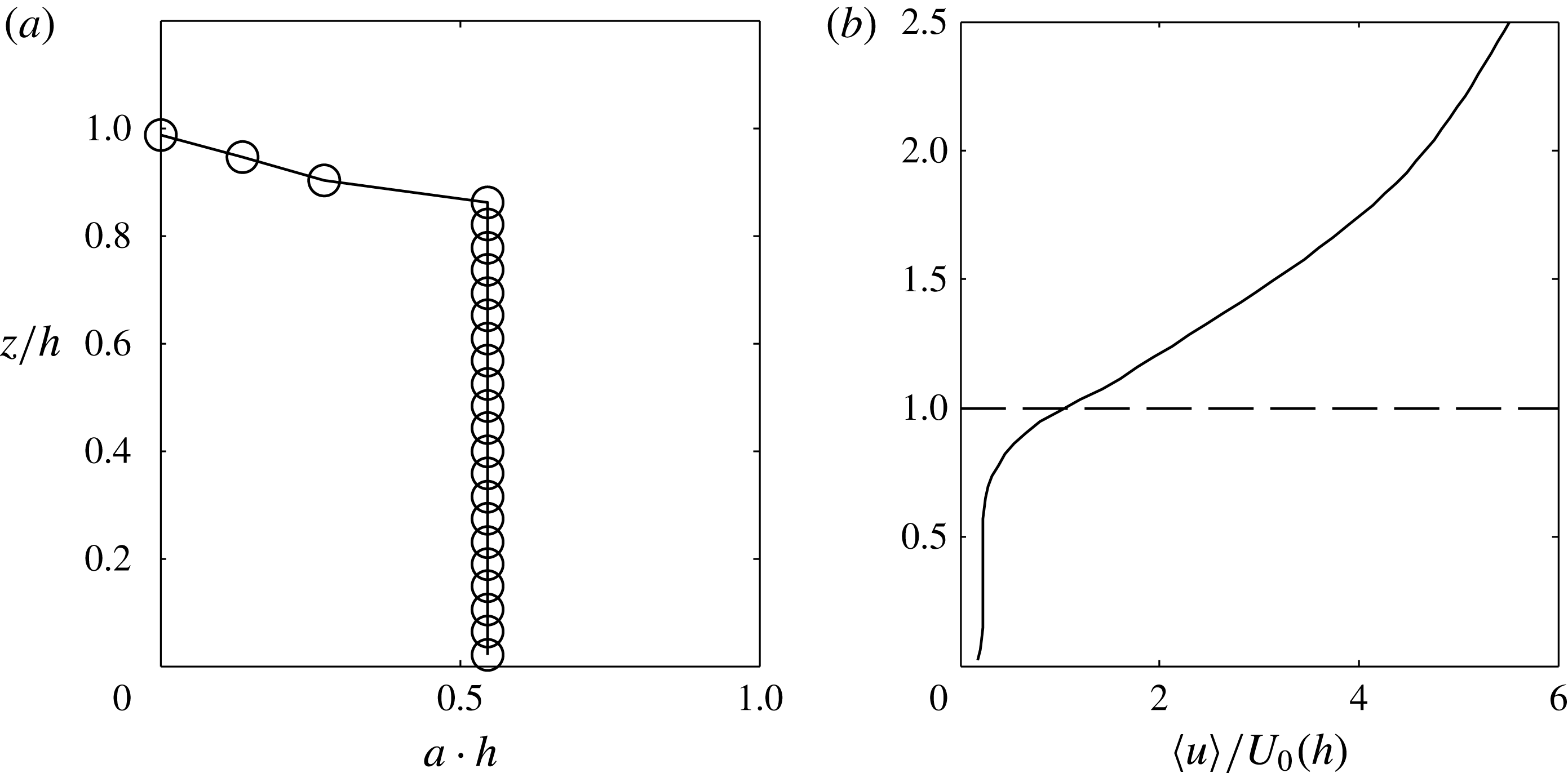
Mean profiles from the start-up simulations. (a) Leaf area density; (b) initial mean velocity profile.

To limit the scales of turbulence, the viscous diffusion term in (2.2) was retained, with the Reynolds number based on canopy height having a value of
 $Re=U_{0}(h)h/{\it\nu}\approx 500$
, where
 $U_{0}(h)$
is the mean initial velocity at the canopy height. The passive scalar was given a Schmidt number of 0.7. (We also tried an infinite Schmidt number and found a minimal impact on results.)
The model canopy extended from the wall to a height of
 $h=L_{z}/4$
and had a leaf area index of 0.5 (figure 1
a) and drag coefficient
 $c_{d}=0.5$
. This gives a dimensionless ‘momentum-absorption parameter’ of
 $c_{d}\,a\,h=0.25$
. The flow was driven with a spatially- and temporally-constant streamwise pressure gradient, which had a value of
 $F_{x}\,h\,U_{0}^{-2}(h)=5.51\times 10^{-5}$
. The computational domain of size
 $L_{x}\times L_{y}\times L_{z}=25h\times 13h\times 4h$
was discretized using a uniform grid of
 $N_{x}\times N_{y}\times N_{z}=192\times 96\times 96$
nodes with spacing
 ${\it\Delta}_{x}\times {\it\Delta}_{y}\times {\it\Delta}_{z}=0.13h\times 0.13h\times 0.04h$
. The numerical grid was fine enough that nearly all turbulent motions were resolved for the duration of the start-up simulations (i.e.
 $C_{s}\rightarrow 0$
). The aerodynamic roughness length used in the lower-wall boundary condition was given a value of
 $z_{o}/h=5\times 10^{-4}$
. A spatially- and temporally-constant scalar source term was added in the canopy to approximately mimic scalar source distributions for heat, moisture, CO
 $_{2}$
, etc. Real scalar source distributions often have high variability in the vertical direction, however, we feel that a vertically homogeneous source profile is sufficient for the purposes of this work.
Domain size and Reynolds number were varied to assess their impact. Substantially increasing horizontal domain extent had a minimal effect on results. Vertical domain height also had a minimal effect on initial development, as the stress had not been given sufficient time to propagate to the domain top and thus structures on the scale of
 $L_{z}$
had not yet formed. Varying Reynolds number changed the degree to which small-scale perturbations developed. For very small Reynolds number, roll up occurred but rollers never broke down into sub-roller scales. Choosing a very large Reynolds number meant that the rollers broke down into smaller scales very quickly, making it difficult to observe structure evolution. We chose an intermediate value which allowed for the formation of grid-scale structures, but that was small enough that the evolution of individual larger-scale structures was identifiable. We also allowed the simulations to run to a quasi-steady state to verify that the domain size was large enough that fully three-dimensional flow with an inertial range would eventually develop.
Flow structures were visualized using isosurfaces of
 ${\it\lambda}_{2}$
(Jeong & Hussein Reference Jeong and Hussein1995), which is the second eigenvalue of
 $\tilde{\unicode[STIX]{x1D61A}}_{ij}^{2}+\tilde{{\it\Omega}}_{ij}^{2}$
, where
 $\tilde{\unicode[STIX]{x1D61A}}_{ij}$
and
 $\tilde{{\it\Omega}}_{ij}$
are, respectively, the symmetric and antisymmetric parts of the filtered velocity-gradient tensor. Jeong & Hussein (Reference Jeong and Hussein1995) argued that connected regions of
 ${\it\lambda}_{2}<0$
are a relatively objective and robust indicator of a vortex. A wide range of vortex definitions have been suggested throughout the literature, each claiming to be more robust and objective than previous definitions in certain situations (e.g. Metcalfe et al.
Reference Metcalfe, Hussain, Menon, Hayakawa, Durst, Launder, Lumley, Schmidt and Whitelaw1985; Hunt, Wray & Moin Reference Hunt, Wray and Moin1988; Zhou et al.
Reference Zhou, Adrian, Balachandar and Kendall1999; Haller Reference Haller2005; Green, Rowley & Haller Reference Green, Rowley and Haller2007). We tried some of these other definitions of a vortex based on the velocity gradient tensor and found that similar conclusions could be drawn regardless of the choice of isosurface variable.
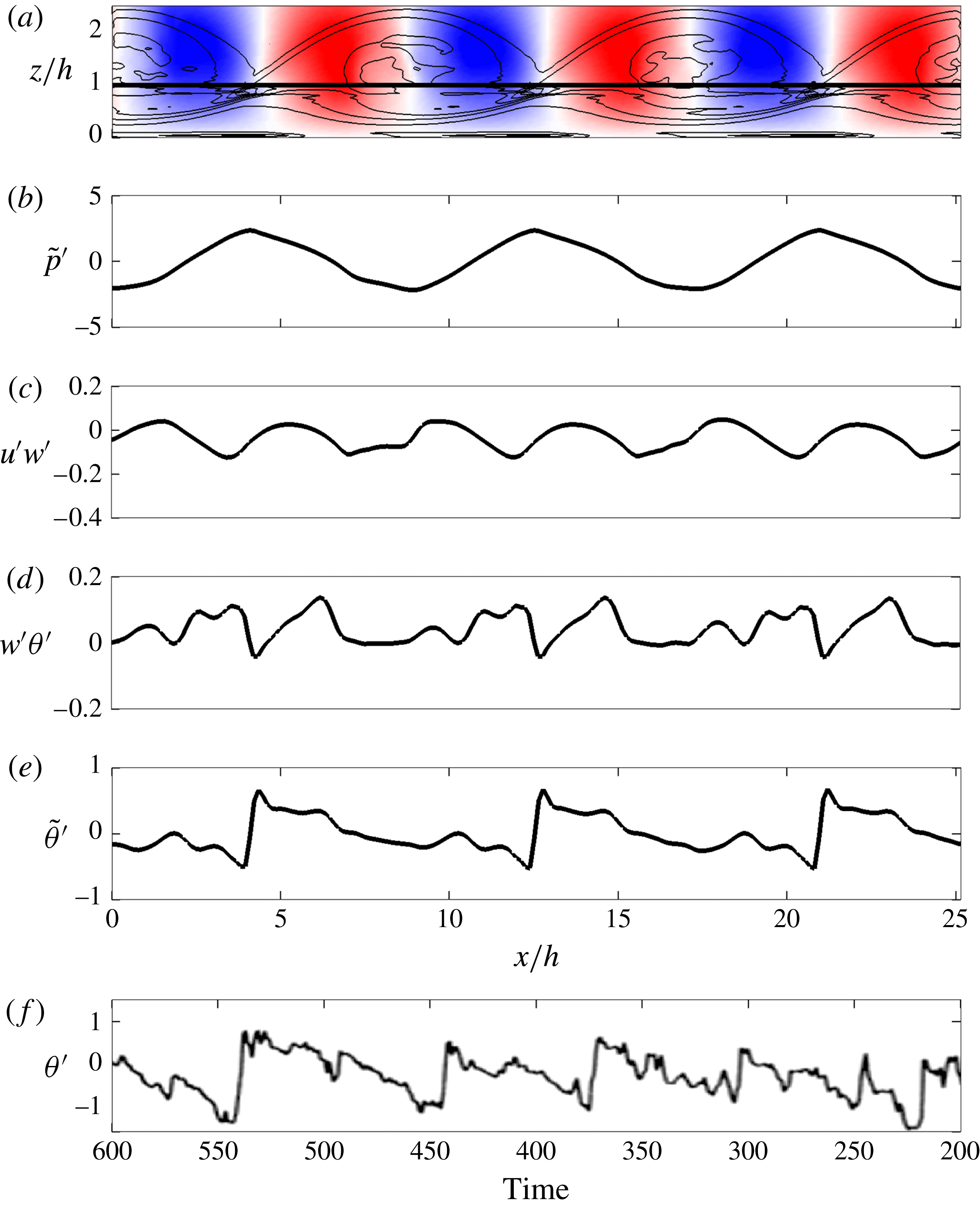
Illustration of scalar microfront structures and their association with pressure and vertical fluxes from the start-up flow after a time of
 $10\,U_{0}(h)/h$
. (a) Spanwise-averaged contours of spanwise vorticity (mean flow from left to right), with positive and negative vertical velocity perturbation shown in red and blue, respectively (range of
 $\pm 0.5~\text{m}~\text{s}^{-1}$
); (b) streamwise transect of
 $\tilde{p}^{\prime }$
from the LES data at
 $z=h$
which corresponds to the solid horizontal line in (a); (c) streamwise transect of Reynolds stress
 $u^{\prime }w^{\prime }$
from the LES data at
 $z=h$
; (d) streamwise transect of scalar flux
 $w^{\prime }{\it\theta}^{\prime }$
from the LES data at
 $z=h$
; (e) streamwise transect of
 $\tilde{{\it\theta}}^{\prime }$
from the LES data at
 $z=h$
; (f) experimental time series of Gao et al. (Reference Gao, Shaw and Paw1989) for fully-developed canopy flow with unstable stratification measured at
 $z/h=0.9$
. Reproduced with kind permission of Springer Science+Business Media. Note that time in (f) increases moving from right to left to allow qualitative comparison with the spatial data in (e).

3.1. Roll up and vertical asymmetry
Previous authors have demonstrated that flows with an inflected velocity profile (e.g. mixing layers) are inviscidly unstable to disturbances of arbitrary wavenumber at all stages of development, with the most unstable being relatively low wavenumbers (Michalke Reference Michalke1965; Huerre & Monkewitz Reference Huerre and Monkewitz1985). As discussed earlier, the mean velocity profile of a canopy layer contains an inflection point at the canopy top which is a result of momentum absorption by canopy elements.
In the start-up canopy simulations (and analogous to mixing-layer flows) roll up occurs rapidly as a result of the growth of low-wavenumber disturbances. The canopy-top velocity inflection causes the formation of characteristic spanwise roller vortices, as illustrated by figure 2(a).
Symmetry is an important feature of mixing layers. The mixing layer grows symmetrically about the mixing plane, and velocity moments are generally symmetric (or antisymmetric) about the mixing plane (Bell & Mehta Reference Bell and Mehta1990; Rogers & Moser Reference Rogers and Moser1994). Previous work has demonstrated that the addition of a wall boundary to a mixing layer acts to break this symmetry (Lindzen & Rosenthal Reference Lindzen and Rosenthal1976; Holt Reference Holt1998). The addition of a boundary acts to displace the roller cores away from the mixing plane toward the unbounded side, although the roller still remains roughly symmetric (Holt Reference Holt1998). Figure 2(a) shows instantaneous contours of spanwise-averaged vorticity
 $\widetilde{{\it\omega}}_{2}=((\partial \tilde{u} /\partial z)-(\partial \tilde{w}/\partial x))$
for the start-up flow. In a free mixing layer, rollers are rotationally symmetric about the mixing plane. In contrast, rollers in the canopy layer are not symmetric about the canopy top (mixing plane). Figure 2(a) shows that the roller core is located at roughly
 $z=1.3h$
–
 $1.4h$
instead of
 $z=h$
as one might expect in symmetric flow. This symmetry breaking is to some degree a result of blocking by the lower wall as in Holt (Reference Holt1998). In the presence of a sufficiently dense canopy, the wall stress is essentially zero and the lower wall is not felt by upper canopy structures. In this case a displaced ‘effective’ wall is created at some height
 $0<z<h$
.
The canopy has an additional feature not present in previous studies of wall-bounded mixing layers, which is distributed momentum absorption by canopy elements. The canopy acts as a momentum sink and damps turbulent motions. Therefore, the portion of roller structures extending into the canopy experiences a non-conservative damping force that is not present above. In both cases, both mechanisms contribute to an asymmetrical eddy structure about the canopy top.
3.1.1. Convective velocity scales
Asymmetry in the eddy structure about the canopy top explains previous observations (e.g. Shaw et al.
Reference Shaw, Brunet, Finnigan and Raupach1995) that convective scales near the canopy are larger than the mean wind velocity. If we accept that (to an inviscid approximation) the roller structure is advected at the speed of the mean flow, we should expect that the mean velocity should match the convective velocity scale at the roller core. For the start-up flow, we estimate through direct observation that the convective velocity of the roller cores is approximately
 $U_{c}\approx 1.5U(h)$
at the time shown in figure 2. If we examine the mean velocity profile at this time, we calculate that the mean flow velocity at the approximate height of the roller cores is
 $U(1.3h)=1.47U(h)$
, which matches the convective velocity of the roller cores. Certainly, there is some uncertainty in the precise height of the roller cores, but this approximation suggests that the mean flow at the height of the displaced roller cores largely determines the convective velocity scale. This agrees with the results of Shaw et al. (Reference Shaw, Brunet, Finnigan and Raupach1995), which show that the convective velocity scale approximately matches the mean flow velocity at
 $z\approx 2.75h$
. It is expected that the roller cores in Shaw et al. (Reference Shaw, Brunet, Finnigan and Raupach1995) will be situated higher than that of the start-up flow because their boundary layer is fully developed. Profiles shown in Shaw et al. (Reference Shaw, Brunet, Finnigan and Raupach1995) show that the streamwise convective velocity scale is relatively constant above
 $z=h$
, and that drag from the canopy reduced the convective scale below
 $z=h$
. This supports our claim that the mean velocity at the roller core height is the most important velocity scale in determining the convective velocity scale, and that drag reduces this velocity inside the canopy.
3.1.2. Sweep-ejection structure
As mentioned previously, asymmetry in the vertical direction has a substantial impact on the ratio of contributions to vertical fluxes by ejections versus sweeps (Baldocchi & Hutchinson Reference Baldocchi and Hutchinson1987; Christen & Vogt Reference Christen and Vogt2004; Finnigan et al. Reference Finnigan, Shaw and Patton2009; Bailey et al. Reference Bailey, Stoll, Pardyjak and Mahaffee2014). Previous work has identified several consistent patterns. Well above the canopy, ejections give larger contributions to vertical fluxes than do sweeps. Near the canopy top and below, the opposite is true, with sweeps dominating ejections. Below the canopy mixing height where vertical fluxes become small, a dominance of ejections over sweeps begins to re-emerge. Finnigan et al. (Reference Finnigan, Shaw and Patton2009) offered an argument based on conjecture that the sweep-ejection structure was due to symmetry breaking in the evolution of head-up and head-down hairpin vortices. The argument was that in a flow with an increasing velocity profile, hairpins deflected downward will experience greater strain than hairpins deflected upward at the same location. They reasoned that the highly strained head-down hairpins (which create sweeps), combined with suppression of upward motions by the wall, lead to a dominance of sweeps near the canopy. Well above the canopy, they said that since upward motions are not constrained by the wall, these motions (ejections) win out over highly strained head-down hairpins which produce sweeps.
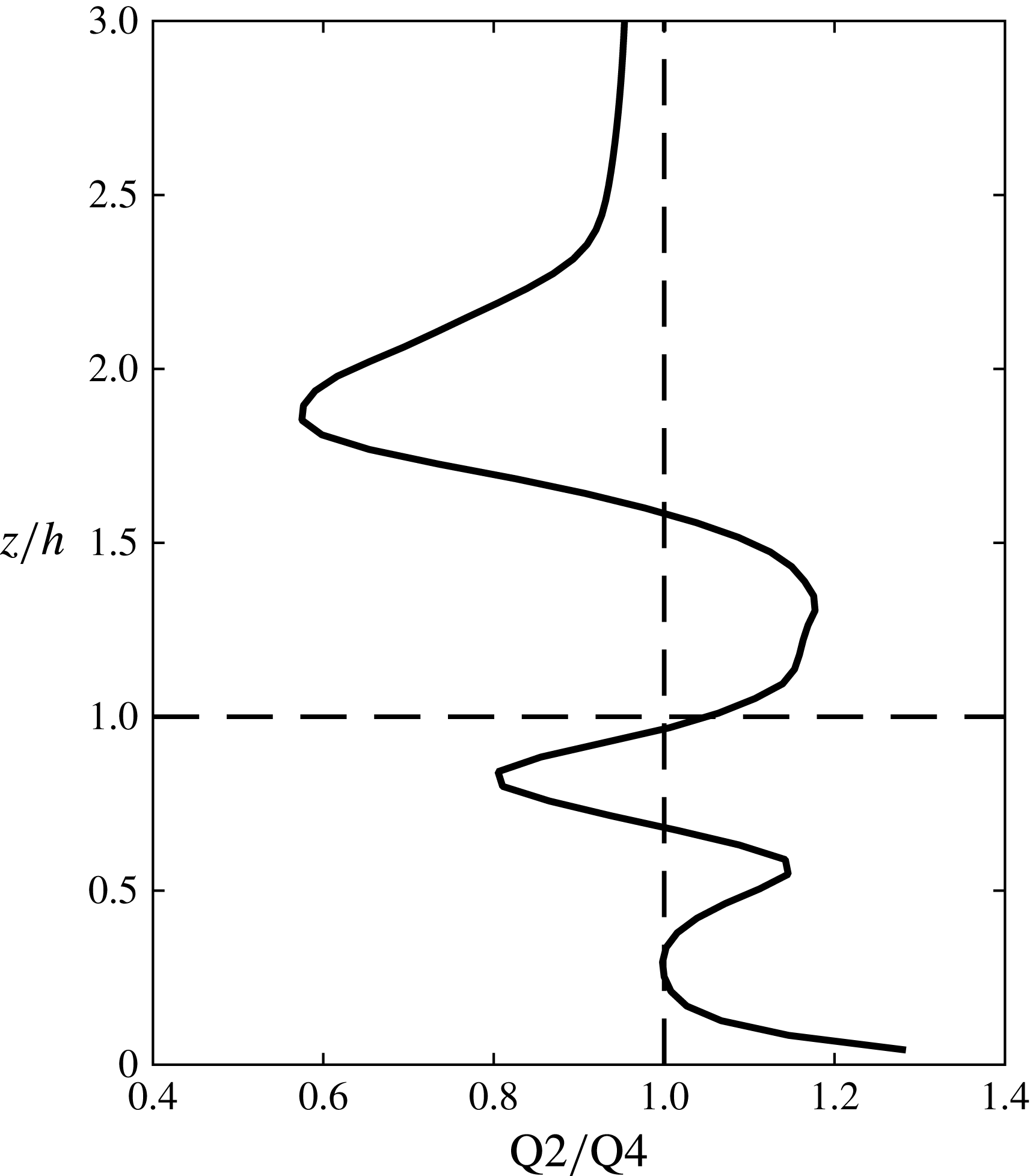
If this is indeed true that head-down hairpins are required for sweep dominance, we should find that in the early stages of the start-up flow, which lack a hairpin structure, ejections should dominate at all vertical levels. To test this, we performed quadrant analysis for the instant of the start-up flow shown in figure 2. Figure 3 gives a profile of the ratio of ejections (Q2;
 $u^{\prime }<0$
,
 $w^{\prime }>0$
) to sweeps (Q4;
 $u^{\prime }>0$
,
 $w^{\prime }<0$
) in terms of their contributions to the vertical momentum flux. When comparing this profile to observations in fully-developed canopy flows, we must be cautious to consider the fact that the turbulence structure is not fully developed, and thus that the effects of the eddy structure are confined to the region near the canopy top.
Profile of the ratio of contributions to the mean vertical flux by ejections (Q2;
 $\tilde{u} ^{\prime }<0$
,
 $\tilde{w}^{\prime }>0$
) to sweeps (Q4;
 $\tilde{u} ^{\prime }>0$
,
 $\tilde{w}^{\prime }<0$
) for the instant of the start-up flow shown in figure 2.

With this in mind, we can identify the common features of real canopy flows. First is a transition from ejection dominance to sweep dominance at the canopy top. Second, is that below the approximate mixing height, we see a transition back to ejection dominance. This can be explained as follows. Consider the sweep and ejection motions resulting respectively from the downwind and upwind sides of a transverse vortex. The ejection side of the structure draws its fluid from within the canopy, which is impeded by high drag as well as blocking by the wall. Conversely, the sweep side of the vortex draws its fluid from the high momentum and unobstructed flow above. Thus, the more powerful sweep motions dominate ejections near the canopy. Moving upward, away from the canopy top, ejection motions are decreasingly impeded by canopy drag, leading to stronger ejections.
In contrast to observed profiles, we also see sweep dominance return far above the canopy top. However, this can be attributed to the fact that the flow is not fully developed. As the vortex structure grows upward, high-momentum fluid is entrained downward into the shear layer, creating a dominance of sweeps. If we allow the start-up flow to run longer, we find that the region of ejection dominance above the canopy grows upward until it eventually reaches the domain top and thus ejections dominate the entire region above the canopy. Similarly, below the canopy top, the region of sweep dominance below the canopy grows downward until an equilibrium is reached (but there is still a small region of ejection dominance near the wall).
All of these observations are consistent with quadrant analysis profiles observed in real, fully-developed canopies. This indicates that the sweep-ejection structure in a canopy layer could be due to a purely two-dimensional structure independent of hairpin formation. There is no reason to suspect that the mechanism argued by Finnigan et al. (Reference Finnigan, Shaw and Patton2009) is not also at work in the fully-developed flow. However, it is likely secondary, as it is not necessary in order to produce the commonly observed sweep-ejection structure.
3.2. Scalar microfronts
As discussed previously, upward, ejection-generating coherent motions near the canopy top are inhibited by the low-flux canopy. However, downward, sweep-generating coherent motions are much stronger as they have a source of free air from above. Consequently, sweeps dominate ejections in the canopy. To satisfy mass or scalar continuity within the canopy, upward ejection events must be more frequent than the more powerful downward sweep events, which has been previously observed in experiments (e.g. Coceal et al. Reference Coceal, Dobre, Thomas and Belcher2007) and is demonstrated by our fully-developed LES (figure 7). In terms of the roller vortices, this means that a larger fraction of the canopy top surface area must be occupied by ejection events than sweep events.
The periodic cycle of sweeps and ejections gives rise to the commonly reported ‘scalar microfront’ structures, or what may be considered unusually large streamwise scalar gradients. Figure 2(e) shows instantaneous scalar perturbations along a streamwise transect at a height of
 $z/h=1$
for the simulated flow. The transect is a spanwise average taken after roughly 10 eddy turnover times from the beginning of the simulation. At this point in the flow evolution, three-dimensionality is very weak and the two-dimensional roller structure dominates the flow (see figure 4 for reference). Contours of the associated spanwise vorticity field are given in figure 2(a) which show the approximate location of the rollers. In the region extending from just upwind of the roller core to approximately midway between the rollers, transport is generally upward. Similarly, downward transport occurs in the region immediately downwind of the roller core.
A microfront occurs at the interface where transport abruptly transitions from downward to upward directions. It is important to note that the microfronts are not necessarily an indicator of a single locally-large vertical momentum flux. Rather they are a signature of opposing vertical fluxes in the upwind and downwind directions (figure 2 d). We confirm that the microfront coincides with local maxima in pressure (figure 2 b), as has been previously reported in other work examining fully-developed flow (Fitzmaurice et al. Reference Fitzmaurice, Shaw, Paw and Patton2004; Finnigan et al. Reference Finnigan, Shaw and Patton2009). Despite the fact that figure 2(e) indicates that the largest streamwise scalar gradients are between the rollers, figure 2(c) suggests that the largest (negative) turbulent stresses are generated in the sweep region upwind of the microfront and at the roller core.
What is additionally striking is the asymmetrical ‘ramp’-like patterns that form. Although scalar traces shown in figure 2(e) are associated with the two-dimensional, temporally-developing flow, they exhibit the classical features of experimental data collected in real canopy flows (e.g. Gao et al. Reference Gao, Shaw and Paw1989; Shaw et al. Reference Shaw, Paw and Gao1989). Figure 2(f) shows a sample scalar time series from the study of Gao et al. (Reference Gao, Shaw and Paw1989), which has a qualitatively similar trend as in the simulated flow. Both signals show a periodic trend of sharp streamwise gradients bracketed on either side by slowly decreasing scalar perturbations and a relatively quiescent zone. This offers compelling evidence that the scalar ramp patterns observed in real canopy flows could be caused by an underlying quasi-two-dimensional roller structure that persists to the fully-developed state.
In contrast to this result, previous studies of canopy structures have associated the microfronts with a more three-dimensional structure, such as the dual hairpin structure of Finnigan et al. (Reference Finnigan, Shaw and Patton2009). Such a three-dimensional structure appears to be supported by two-point correlation measurements performed by Shaw et al. (Reference Shaw, Brunet, Finnigan and Raupach1995), which found that the spanwise correlation scale is of order
 $h$
rather than the spanwise flow extent. However, it has been well documented that even slight irregularities in a predominantly spanwise structure can result in very low spanwise correlation scales. Browand & Troutt (Reference Browand and Troutt1980) and Browand & Troutt (Reference Browand and Troutt1985) demonstrated this fact for a predominantly two-dimensional mixing layer. Hutchins & Marusic (Reference Hutchins and Marusic2007) found that meandering of streamwise structures severely affected length scales inferred from two-point correlation measurements. We suspect that the near-canopy flow is dominated by a predominantly two-dimensional structure that contains irregularities. We certainly do not contend that the flow does not contain three-dimensionality. The presence of an approximate
 $k^{-5/3}$
kinetic energy spectrum observed in both fully-developed mixing and canopy layers (e.g. Huang & Ho Reference Huang and Ho1990; Finnigan Reference Finnigan2000) implies that the flow is fully three-dimensional. However, our claim is that underlying two-dimensional motions dominate near-canopy flow and are largely responsible for the scalar ramp structures. We now seek to more closely examine the role of three-dimensionality in the structure of the flow.
3.3. Development of three-dimensionality
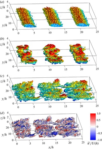
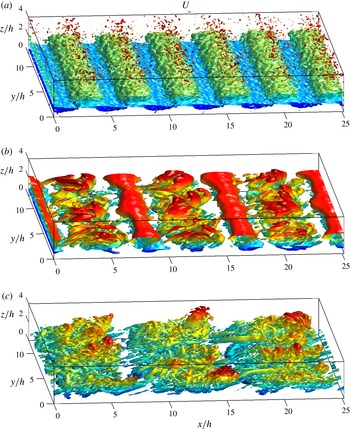
As the start-up flow progresses, vortex breakdown occurs and smaller turbulent scales appear, as illustrated by the temporal progression shown in figure 4. At this point, the rollers are no longer well-defined vortex tubes as one may envision in the traditional sense. Rather, they are underlying vortical motions that transport smaller vortices in a circular motion. This process is similar to that observed in traditional mixing-layer studies (e.g. Tanahashi, Iwase & Miyauchi Reference Tanahashi, Iwase and Miyauchi2001; Wang, Tanahashi & Miyauchi Reference Wang, Tanahashi and Miyauchi2007). It is perhaps because of this fact that in flows with very high Reynolds numbers, Kelvin–Helmholtz rollers are usually referred to as ‘billows’ rather than vortices. Localized vortex sheets are generated by neighbouring structures, which can then undergo higher-order roll up, sustaining a self-similar structure (Moser & Rogers Reference Moser and Rogers1991).
Progression of the start-up simulations as shown by isosurfaces of
 ${\it\lambda}_{2}$
. Isosurfaces are coloured by vertical height for visual clarity. Mean flow is from left to right. Panels show different stages of flow progression: (a)
 $t\,(U_{0}(h)/h)=1.23$
,
 ${\it\lambda}_{2}=-0.1$
; (b)
 $t\,(U_{0}(h)/h)=16.8$
,
 ${\it\lambda}_{2}=-40$
; (c)
 $t\,(U_{0}(h)/h)=18.5$
,
 ${\it\lambda}_{2}=-200$
. Frame (d) is the same as (c), except that isosurfaces are coloured by
 $\tilde{u} ^{\prime }/U(h)$
. An animation of the start-up simulation can be found in the online supplemental material (see supplementary movie 1 available at http://dx.doi.org/10.1017/jfm.2015.749).

As is required by the vorticity equation, vortex lines must continually stretch. Given sufficient time and a large enough Reynolds number, they are likely to form inclined arched or hairpin-like structures (Robinson Reference Robinson1991; Gerz et al. Reference Gerz, Howell and Mahrt1994). The precise inclination angle is flow-dependent and is the point when stretching, mean rotation and induced flow are in equilibrium (Rogers & Moin Reference Rogers and Moin1987). Gerz et al. (Reference Gerz, Howell and Mahrt1994) and Rogers & Moin (Reference Rogers and Moin1987) found in homogeneous turbulence and free shear flow, respectively, that hairpins tended to form in head-up and head-down vortex pairs. Accordingly, they also reported a relatively equal probability of detecting head-up and head-down hairpins. It is not surprising that they found equal probabilities of head-up and head-down hairpins given the symmetry of homogeneous and free shear flows.
As discussed previously, the wall breaks vertical symmetry and thus it would not be surprising to find preferential hairpin formation. In fact many previous workers have reported a more asymmetric hairpin vortex structure in the ISL, which leads to the dominance of head-up hairpin formation (cf. Adrian Reference Adrian, Venditti, Best, Church and Hardy2013).
Figure 4(c,d) shows that after the primary roller structures break down into smaller scales, the underlying two-dimensional structures remain. However, a highly three-dimensional structure also emerges as smaller vortices are stretched and strained, with the two evolving somewhat independently. This feature has been frequently reported in the late development of mixing layers (Browand & Troutt Reference Browand and Troutt1980, Reference Browand and Troutt1985; Lasheras & Choi Reference Lasheras and Choi1988). Superposed on the two-dimensional structure is an array of highly three-dimensional smaller-scale structures. Stretching combined with straining by the primary structures creates a convoluted entwinement of vortices. As is ubiquitously reported in mixing layers, initially spanwise structures stretch and are strained by the primary rollers to create arch- or hairpin-like structures oriented in the streamwise direction (Lasheras & Choi Reference Lasheras and Choi1988; Rogers & Moser Reference Rogers and Moser1992). Arched structures with their heads oriented downward and behind their legs are strained downward and against the mean streamwise flow. Their vertical progression is impeded by a combination of canopy drag and the wall (or displaced wall), but they still may form hairpins due primarily to horizontal straining. Head-up structures on the other hand are strained upward, and are not immediately bounded from above. Thus, we find that they are able to continue stretching upward into a classical boundary-layer hairpin, in many cases extending several canopy heights tall in the vertical.
We notice that the tallest head-up hairpins tend to form along common streamwise transects. For this particular flow, they are at
 $y=0=L_{y}$
and
 $y=L_{y}/2$
. If we colour the isosurfaces by streamwise velocity perturbation (figure 4
d), we find a distinctly ‘streaked’ pattern in the streamwise direction. The streaky patterns can also be confirmed by examining short time averages of the flow (not shown). This streamwise streaky structure that persists over very long streamwise distances has been well documented in mixing layers (Breidenthal Reference Breidenthal1978; Bernal et al.
Reference Bernal, Breidenthal, Brown, Konrad and Roshko1979; Rogers & Moser Reference Rogers and Moser1992) and smooth-walled boundary layers (Kim & Adrian Reference Kim and Adrian1999; Jiménez, Álamo & Flores Reference Jiménez, Álamo and Flores2004; Hutchins & Marusic Reference Hutchins and Marusic2007; Reynolds et al.
Reference Reynolds, Hayden, Castro and Robins2007). In rough-walled boundary layers, enhanced mixing can distort the instantaneous streaks, but they have still been observed in temporal- and composite-averaged fields (Coceal et al.
Reference Coceal, Dobre, Thomas and Belcher2007; Barros & Christensen Reference Barros and Christensen2014; Fang & Porté-Agel Reference Fang and Porté-Agel2015). Persistent mean streamwise low-momentum streaks (manifesting themselves as weak streamwise vortices) have also been found in fully-developed canopy flows (Brunet et al.
Reference Brunet, Finnigan and Raupach1994; Finnigan et al.
Reference Finnigan, Shaw and Patton2009; Bailey & Stoll Reference Bailey and Stoll2013; Perret & Ruiz Reference Perret, Ruiz, Venditti, Best, Church and Hardy2013) (this will be further explored in § 5.4).
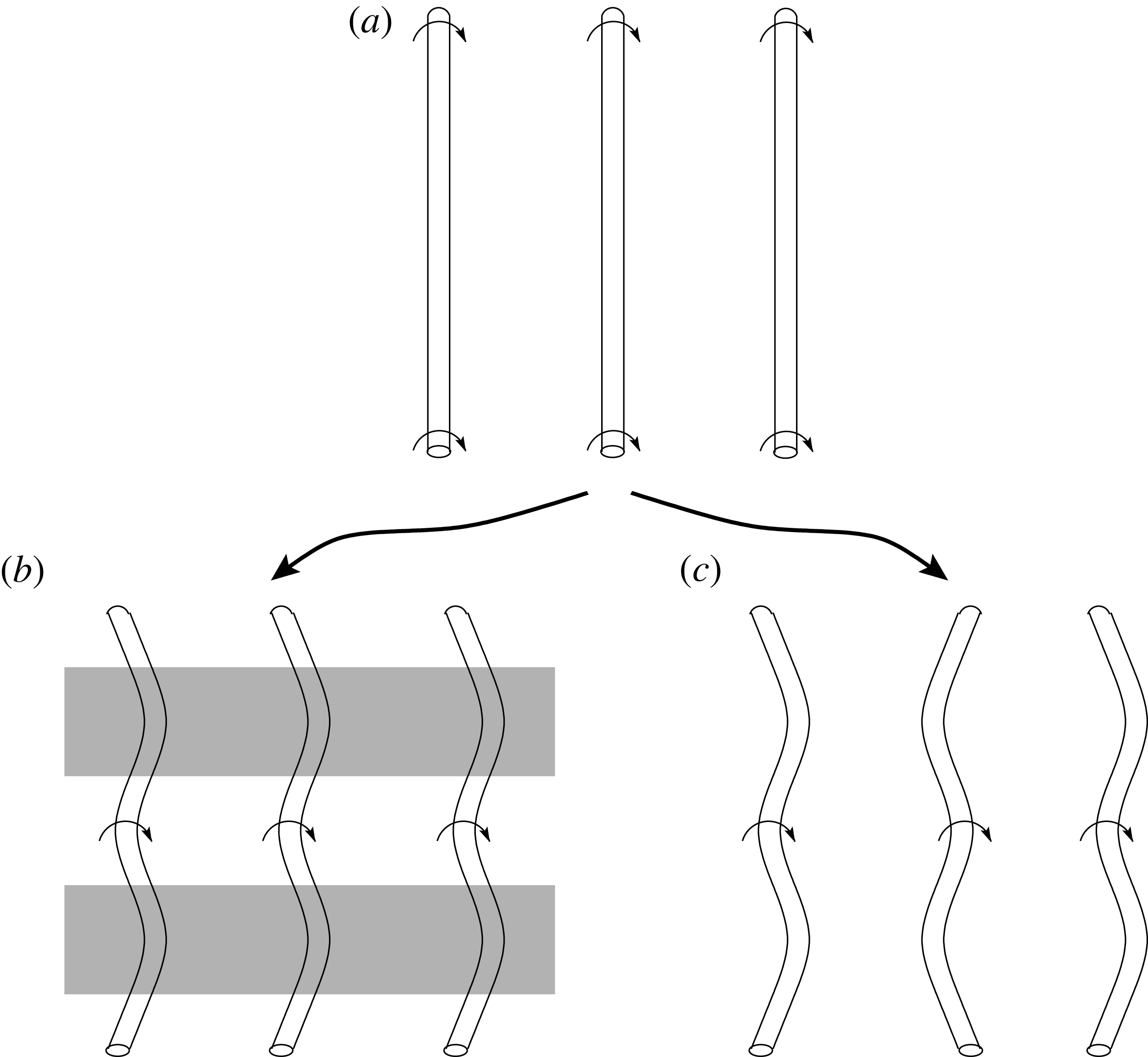
In the case of the mixing layer, these streaks are thought to originate from a secondary-instability mechanism which eventually causes vortices to become strained in the streamwise direction (Lin & Corcos Reference Lin and Corcos1984; Rogers & Moser Reference Rogers and Moser1992). When perturbations of streamwise vortices are in phase between adjacent rollers, they induce upward transport, resulting in streaks of low-momentum fluid. This in-phase formation of streamwise structures is commonly referred to as the ‘translative instability’ (Pierrehumbert & Widnall Reference Pierrehumbert and Widnall1982), which is depicted in figure 5 b). As stressed by Rogers & Moser (Reference Rogers and Moser1992), this is not exclusively a core instability (as in figure 5 b) but rather an instability of the whole flow which may contain sub-roller scales. Out-of-phase displacements, termed ‘helical pairing’, were also explored by Pierrehumbert & Widnall (Reference Pierrehumbert and Widnall1982). As depicted in figure 5(c), this mode of instability does not result in streamwise streaks because transport is vertically symmetric along a streamwise transect. Both the translative and helical pairing instabilities have been commonly observed during early evolution of the flow. Which of these two that dominates early stages the flow is sensitive to initial perturbations (Comte, Lesieur & Lamballais Reference Comte, Lesieur and Lamballais1992; Collis et al. Reference Collis, Lele, Moser and Rogers1994). The helical pairing modes are not unstable to high-wavenumber disturbances, while the translative instability is more broadband in nature (Pierrehumbert & Widnall Reference Pierrehumbert and Widnall1982). Pierrehumbert & Widnall (Reference Pierrehumbert and Widnall1982) investigated the persistence of these two instabilities into later flow development. They found that, although the helical pairing instability could be more amplified initially, it tends to die off with further flow development as pairing occurs and smaller scales emerge. Conversely, the translative instability was found to persist into later flow development, as it is still highly unstable for high-frequency perturbations. There is experimental evidence to suggest that it is the translative instability that dominates the late evolution of mixing-layer flow. The first is the observed phenomenon of streamwise streaks (Browand & Troutt Reference Browand and Troutt1980, Reference Browand and Troutt1985; Lasheras & Choi Reference Lasheras and Choi1988). Secondly, several authors have found that features of later flow evolution quantitatively agreed with the translative instability (Huang & Ho Reference Huang and Ho1990; Rogers & Moser Reference Rogers and Moser1992; Comte, Silvestrini & Bégou Reference Comte, Silvestrini and Bégou1998). For example, Huang & Ho (Reference Huang and Ho1990) found that spanwise length scales agreed with predictions of Pierrehumbert & Widnall (Reference Pierrehumbert and Widnall1982) for the translative instability. Rogers & Moser (Reference Rogers and Moser1992) found that growth rates of unstable modes corresponded to that of the translative instability. To our knowledge, no previous work has reported the dominance of the helical pairing instability for late evolution of a mixing layer (i.e. after full transition to turbulence has occurred).
Illustration of three-dimensional vortex instabilities in mixing-layer flows (flow is from left to right). Vortex structures start as predominantly spanwise (a), then may evolve according to the translative instability (b) or the helical pairing instability (c). Shaded (unshaded) areas in (b) indicate regions of low-speed (high-speed) streaks in streamwise velocity.

Similarly, in boundary-layer flows, Klebanoff, Tidstrom & Sargent (Reference Klebanoff, Tidstrom and Sargent1962) originally noted the presence of a secondary instability that could lead to in-phase displacements of primarily spanwise structures corresponding to harmonic modes, which is usually referred to as a K-Type instability. This mode of instability has been reported to result in ‘peak-valley splitting’, which is qualitatively similar to what we described above for the translative instability of mixing layers (Klebanoff et al. Reference Klebanoff, Tidstrom and Sargent1962; Saric & Thomas Reference Saric, Thomas and Tatsumi1984; Herbert Reference Herbert1988). Boundary layers also have a helical pairing analogue with out-of-phase displacements corresponding to sub-harmonic modes (Herbert Reference Herbert1988). As in mixing layers, the selection of in-phase and out-of-phase instability is sensitive to initial conditions. Most studies have examined secondary instability in terms of its influence on the transition to turbulence. From a theoretical perspective, it is unclear which secondary-instability modes dominate the fully-developed boundary layer, however the presence of persistent streamwise streaks suggests a dominance of in-phase (harmonic) secondary instability.
In mixing layers, the spanwise wavelength of these streaks is slightly less than the primary roller spacing (about
 $(2/3){\it\Lambda}_{x}$
; Pierrehumbert & Widnall Reference Pierrehumbert and Widnall1982; Huang & Ho Reference Huang and Ho1990). In boundary layer and canopy flows, the wavelength of the streaks is of the order of the boundary-layer height
 ${\it\delta}$
(Hutchins & Marusic Reference Hutchins and Marusic2007; Finnigan et al.
Reference Finnigan, Shaw and Patton2009). We find from the start-up flow that the wavelength of the streaks is roughly equal to
 $L_{z}$
or
 ${\it\delta}$
. The study of Ghisalberti (Reference Ghisalberti2010) regarding the structure of an aquatic canopy also revealed what looks like in-phase displacements of spanwise structures, with a spanwise wavelength of about the boundary-layer height. Since spanwise length scales follow the same scaling for canopy and boundary layers, this would suggest that outer-layer instability is modulating the mean spanwise structure in the canopy layer. We find that the tallest hairpins tend to form in streamwise streaks of low streamwise velocity. Since the spanwise spacing between the streaks is consistent with instability in the overlying boundary layer, it would appear the secondary instability in the boundary layer creates a streaky structure that favours the formation of head-up hairpins. The work of Comte et al. (Reference Comte, Lesieur and Lamballais1992) also discussed how hairpin formation would be favoured in troughs of vorticity and inhibited in crests. This is consistent with observations in the ISL of hairpin packets coinciding with very long streaks in low-momentum fluid (Hommema & Adrian Reference Hommema and Adrian2003; Hutchins & Marusic Reference Hutchins and Marusic2007). As was also suggested by Hutchins & Marusic (Reference Hutchins and Marusic2007), it is conceivable that outer scaling modulates structure cycles in the roughness layer. We claim that alternating outer-layer patterns in the momentum field favours the evolution of predominantly spanwise structures near the canopy into hairpin structures that propagate into the overlying ISL. This process also agrees with Townsend’s attached-eddy hypothesis which states that inner and outer-layer structures are not independent.
4. Conceptual model
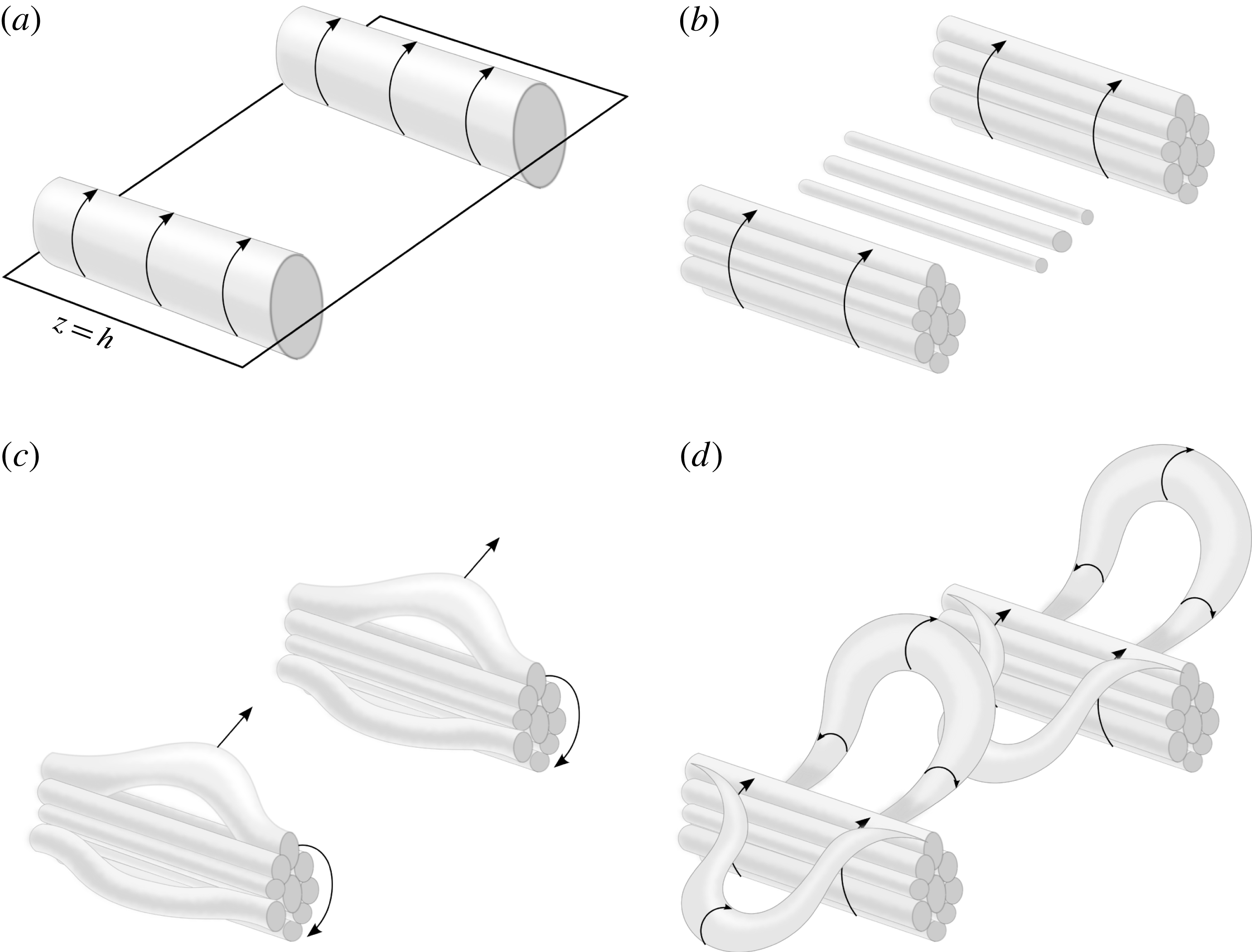
The results of the previous section are summarized into a compact phenomenological model that describes the production and evolution of coherent structures in canopy flow. It is presumed at this point that this same basic chain of events still occurs in the fully-developed quasi-steady flow (providing further evidence for this is the objective of the remainder of the paper). However, it should be noted that in the fully-developed flow, such a chain of events is likely to take place continuously and at many scales. Each stage of the model is depicted by a separate frame in figure 6. It should be stressed that conceptual sketches generally necessitate a simplistic view of very complex processes. This is especially true regarding the smaller-scale structures depicted in the sketch, which evolve over a very wide range of scales and continuously in time.
A conceptual schematic of the creation and evolution of coherent structures in plant canopy flow. (a) Spanwise rollers arising from the Kelvin–Helmholtz instability form asymmetrically about the canopy top. (b) As the full range of length scales forms, the rollers break down to form a conglomeration of smaller vortices. (c) Sub-roller scale vortices stretch and kink to form head up and head-down arch structures, which are usually in phase between adjacent rollers. (d) As the upper vortices stretch, they form a hairpin structure whose legs are rotated below the rollers. Head-down vortices are constrained by the canopy, whereas head-up hairpins continually stretch and eventually break up, allowing the cycle to repeat.

(a) Asymmetric roll up and diffusion: As a result of the inflected mean velocity profile, Kelvin–Helmholtz waves grow and eventually roll up to form spanwise roller vortices. The roll up occurs at a wavelength corresponding to the most unstable modes dictated by the level of canopy-top shear. Because of strong momentum absorption by canopy elements or the wall at the lower boundary, shear is asymmetric about the canopy top. Therefore, vorticity in the rollers diffuses asymmetrically in the vertical direction. This is the underlying structure that dominates flow near the canopy, and causes ‘microfront’ patterns in scalar time traces.
(b) Small-scale structure: Spanwise roller vortices break down to form the full range of turbulent length scales. The rollers are not well-defined vortices. Rather, they are purely conceptual and represent a net vortical motion that transports a range of smaller vortices in a circular pattern. Mean shear and local vortex sheets sustain local roll up of self-similar structures.
(c) Development of three-dimensionality: As predominantly spanwise vortices elongate due to stretching and straining, they deform three-dimensionally. Vortices kink due to vortex stretching, and are strained between larger-scale roller motions.
(d) Hairpin formation: Secondary instability in the overlying ISL modulates the formation of near-canopy hairpins, favouring the progression of hairpins along certain streamwise transects, and inhibiting them along others. Because they are relatively un-bounded from above, vortices stretching upward are continually lifted, stretched and tilted. This creates a head-up hairpin vortex structure linking the roughness layer to the above ISL. The head-down vortices are constrained by canopy drag as well as the wall, which inhibits their vertical progression.
 ${\hookrightarrow}(\mathit{a})$
. Recycling: Mean shear and local vortex sheets sustain the production and break down of spanwise vorticity and an underlying quasi two-dimensional roller structure. This allows the processes to repeat indefinitely. Head-up hairpins are further lifted and stretched, with the upper portions eventually losing correlation with their corresponding roller.
5. The quasi-steady canopy layer
The previous sections provided a basis for understanding coherent structure evolution through visualization of a temporally-evolving canopy layer. However, the overall goal of this study is to understand the structure of fully-developed canopy flows. An extension of the start-up flow to the fully-developed flow was made primarily through conjecture, which was supported by the results of previously published work. In this section, we seek to generate new evidence from a fully-developed canopy layer simulation to support the claims of the previous sections. This is more difficult than in the developing flow, as the wide range of length scales produces a convoluted flow that makes it nearly impossible to obtain meaningful visualizations of the instantaneous flow field. Consequently, we resort to composite-averaging techniques to visualize composite or ‘characteristic’ structures.
Two domain sizes were considered for the simulations. The smaller of the two domains was
 $L_{x}\times L_{y}\times L_{z}=29h\times 29h\times 10h$
which was discretized using a uniform grid of
 $N_{x}\times N_{y}\times N_{z}=288\times 288\times 96$
nodes. To assess the impacts of domain size, a second larger simulation was run with
 $L_{x}\times L_{y}\times L_{z}=58h\times 58h\times 20h$
and
 $N_{x}\times N_{y}\times N_{z}=576\times 576\times 192$
. We observed negligible differences in results between the two domain sizes. All results presented below are from the larger domain case.
The flow was driven with a spatially-uniform streamwise pressure gradient that maintained a constant mean mass flux. The aerodynamic roughness length used in the lower wall boundary condition was given a value of
 $z_{o}/h=5\times 10^{-4}$
. The LAD profile was specified the same as in the start-up flow (figure 1
a). Also note that the quasi-steady simulations do not include molecular diffusion terms (i.e.
 ${\it\nu}={\it\alpha}_{{\it\theta}}=0$
). The passive scalar field
 ${\it\theta}$
was initialized as zero everywhere, with a constant source distribution in the canopy as in the start-up flow. The flow was allowed to reach a quasi-steady state before any analysis began.
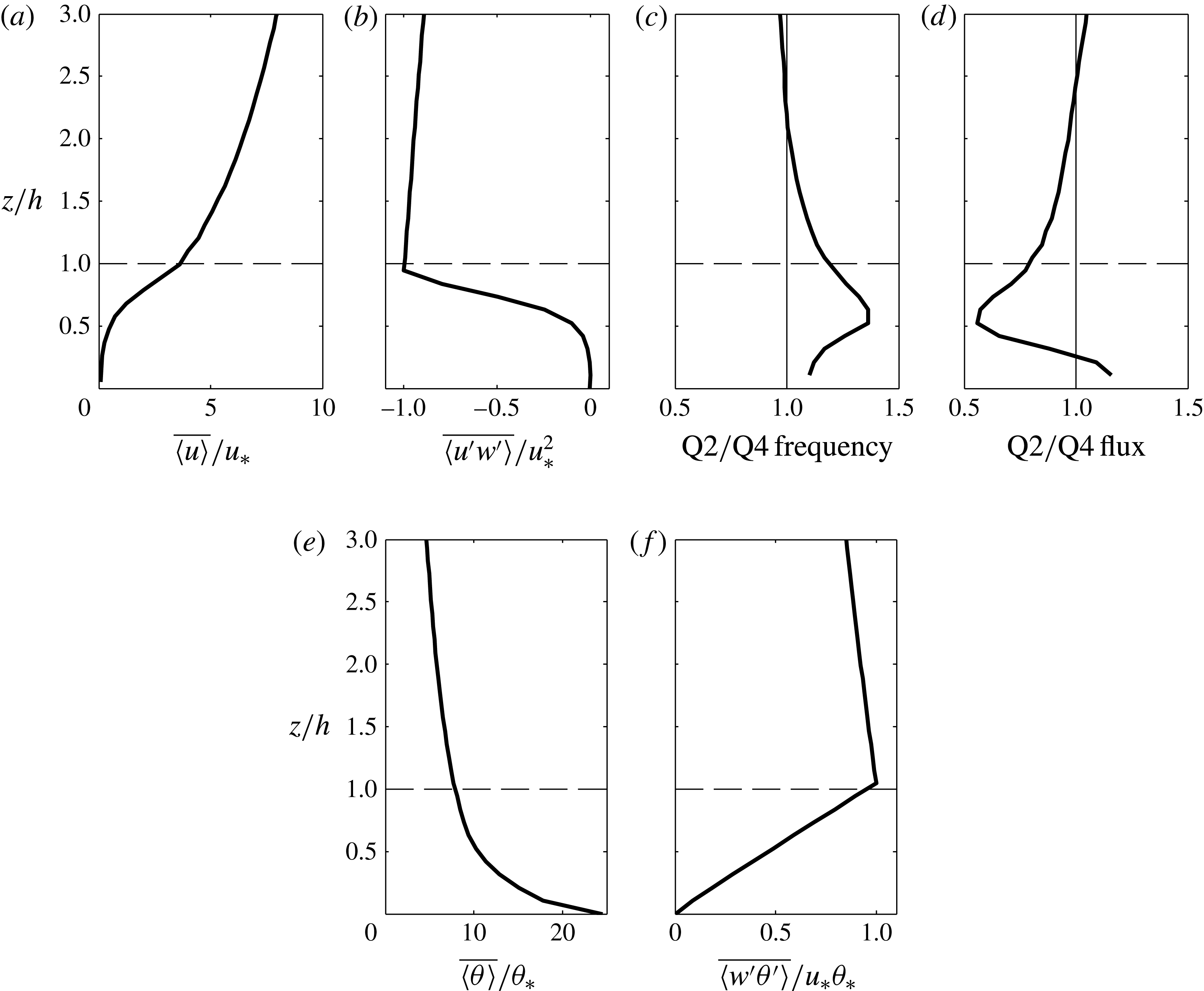
Plane-averaged statistics for the fully-developed flow are given in figure 7. Profiles of the mean streamwise velocity and momentum flux normalized by the shear velocity scale
 $u_{\ast }$
are shown in figure 7(a,b).
 $u_{\ast }^{2}$
was defined here as the maximum value of
 $\big|\overline{\langle u^{\prime }w^{\prime }\rangle }\big|$
. Figure 7(c,d) show standard quadrant analysis profiles with a hole size of 0 (Lu & Willmarth Reference Lu and Willmarth1973). Figure 7(c) is the ratio of the frequency of quadrant 2 (ejection) events to quadrant 4 (sweep) events, and figure 7(d) gives the relative contributions of ejection to sweep events to
 $\overline{\langle u^{\prime }w^{\prime }\rangle }$
. These profiles demonstrate the previous assertion that within the canopy layer, ejection events are more frequent, whereas sweep events give greater contributions to the momentum flux. Above the canopy layer, the opposite is true. The mean scalar and vertical scalar flux profiles are given in figure 7(e,f). Profiles are normalized by
 ${\it\theta}_{\ast }=\text{max}(\overline{\langle w^{\prime }{\it\theta}^{\prime }\rangle })/u_{\ast }$
. The mean scalar decreases monotonically with height, which results in a positive mean vertical scalar flux throughout the domain.
Plane-averaged statistics from the fully-developed simulations: (a) normalized streamwise velocity; (b) normalized momentum flux; (c) ratio of the frequency of Q2 (ejection) to Q4 (sweep) events; (d) ratio of contributions to the momentum flux by Q2 to Q4 events; (e) normalized mean scalar profile; (f) normalized mean vertical scalar flux.

5.1. Conditional averaging methodology
In order to educe the structure of a characteristic eddy, we largely followed the conditional averaging methodology of Finnigan et al. (Reference Finnigan, Shaw and Patton2009), which can be summarized as follows. We define a generic Eulerian variable
 ${\it\phi}(x_{i};t)$
as a trigger for conditionally sampling of the flow. The trigger variable was chosen such that when it is between some threshold range
 ${\it\alpha}_{min}$
and
 ${\it\alpha}_{max}$
, it presumably coincides with the presence of a turbulent structure of interest. To constrain the length scale of the structure, the trigger was only examined at a fixed vertical level of the flow
 $z_{T}$
. Thus at various instances of the flow,
 ${\it\phi}$
was searched for instances where
 ${\it\alpha}_{min}<{\it\phi}(x,y,z_{T};t)<{\it\alpha}_{max}$
. Local maxima of
 ${\it\alpha}_{min}<{\it\phi}<{\it\alpha}_{max}$
were identified, and their planar coordinates
 $\{x_{T},\,y_{T}\}$
noted. To help ensure threshold crossings were independent, smaller maxima within some specified radius of a larger local maxima were discarded. At each remaining local maximum, a realization of the flow was extracted (
 $\tilde{u} ,\,\tilde{v},\,\tilde{w},\,\tilde{p},\,{\it\lambda}_{2}$
), which was centred about
 $\{x_{T},\,y_{T}\}$
. Each realization was averaged to form a composite view of the flow when the threshold was exceeded.
In a similar manner as Finnigan et al. (Reference Finnigan, Shaw and Patton2009), we visualized the time evolution of the composite eddy structure. At each instance of a triggering event (time
 $t_{T}$
), we also looked forward and backward in time at a fixed volume (centred in space at
 $\{x_{T},\,y_{T}\}$
and in time at
 $t_{T}$
). The volumes were then composite averaged at times before and after
 $t_{T}$
to give the temporal evolution of the composite eddy.
5.2. Pressure maxima trigger
We begin by re-examining the composite averaging trigger of Finnigan et al. (Reference Finnigan, Shaw and Patton2009), which takes
 ${\it\phi}=\tilde{p}^{\prime }$
, with
 ${\it\alpha}_{min}=c_{min}u_{\ast }^{2}$
and
 ${\it\alpha}_{max}=c_{max}u_{\ast }^{2}$
(
 $c_{min}$
and
 $c_{max}$
are positive constants). One reason this trigger was suggested by Finnigan et al. (Reference Finnigan, Shaw and Patton2009) is because previous work found that positive peaks in pressure generally coincide with scalar microfronts (Fitzmaurice et al.
Reference Fitzmaurice, Shaw, Paw and Patton2004), which are presumably indicators of high flow coherence or structure.
Our methodology here differs slightly from Finnigan et al. (Reference Finnigan, Shaw and Patton2009) in that we visualize the total velocity field
 $\tilde{u} _{i}$
rather than the perturbation velocity field
 $\tilde{u} _{i}^{\prime }$
. Finnigan et al. (Reference Finnigan, Shaw and Patton2009) visualized their flow using perturbation velocity vectors, and
 ${\it\lambda}_{2}$
calculated from the perturbation velocity field (
 $\tilde{u} ^{\prime },\,\tilde{v}^{\prime },\,\tilde{w}^{\prime }$
). By using perturbation quantities to calculate
 ${\it\lambda}_{2}$
(we denote this as
 ${\it\lambda}_{2}^{\prime }$
), Finnigan et al. (Reference Finnigan, Shaw and Patton2009) removed the mean vorticity
 $\partial \langle u\rangle /\partial z$
, and thus their composite structure corresponds to the perturbation vorticity field. Their approach has several potential pitfalls. One is that it could possibly remove a structure in which the mean vorticity plays a major role. Secondly, it can introduce spurious structures that are not present in the actual velocity field. We have chosen to use the total vorticity field in this section to eliminate these possible issues. However, we further explore the consequences of visualizing structures using the perturbation velocity and vorticity field in the Appendix.
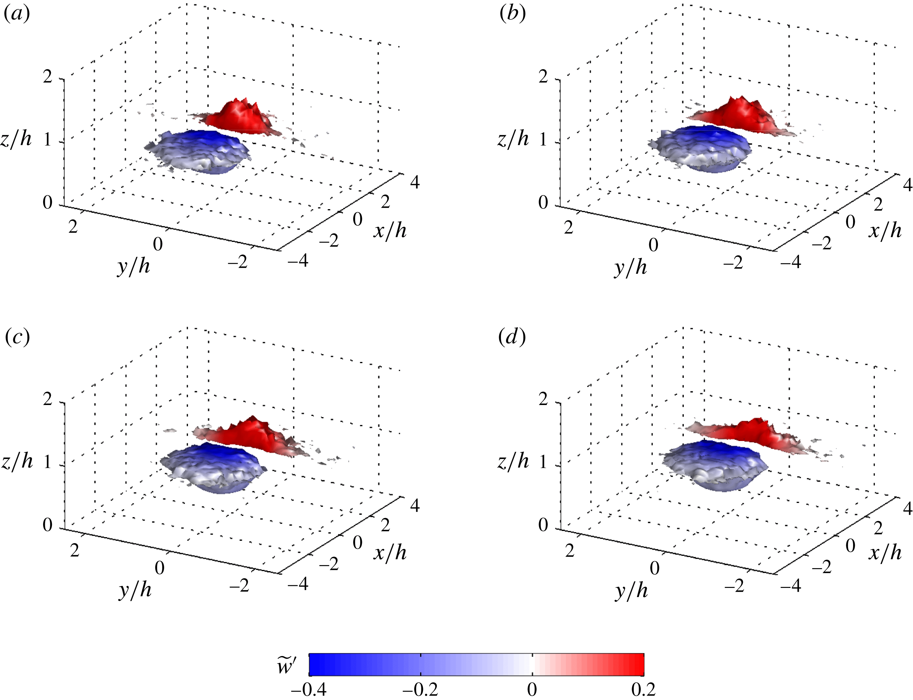
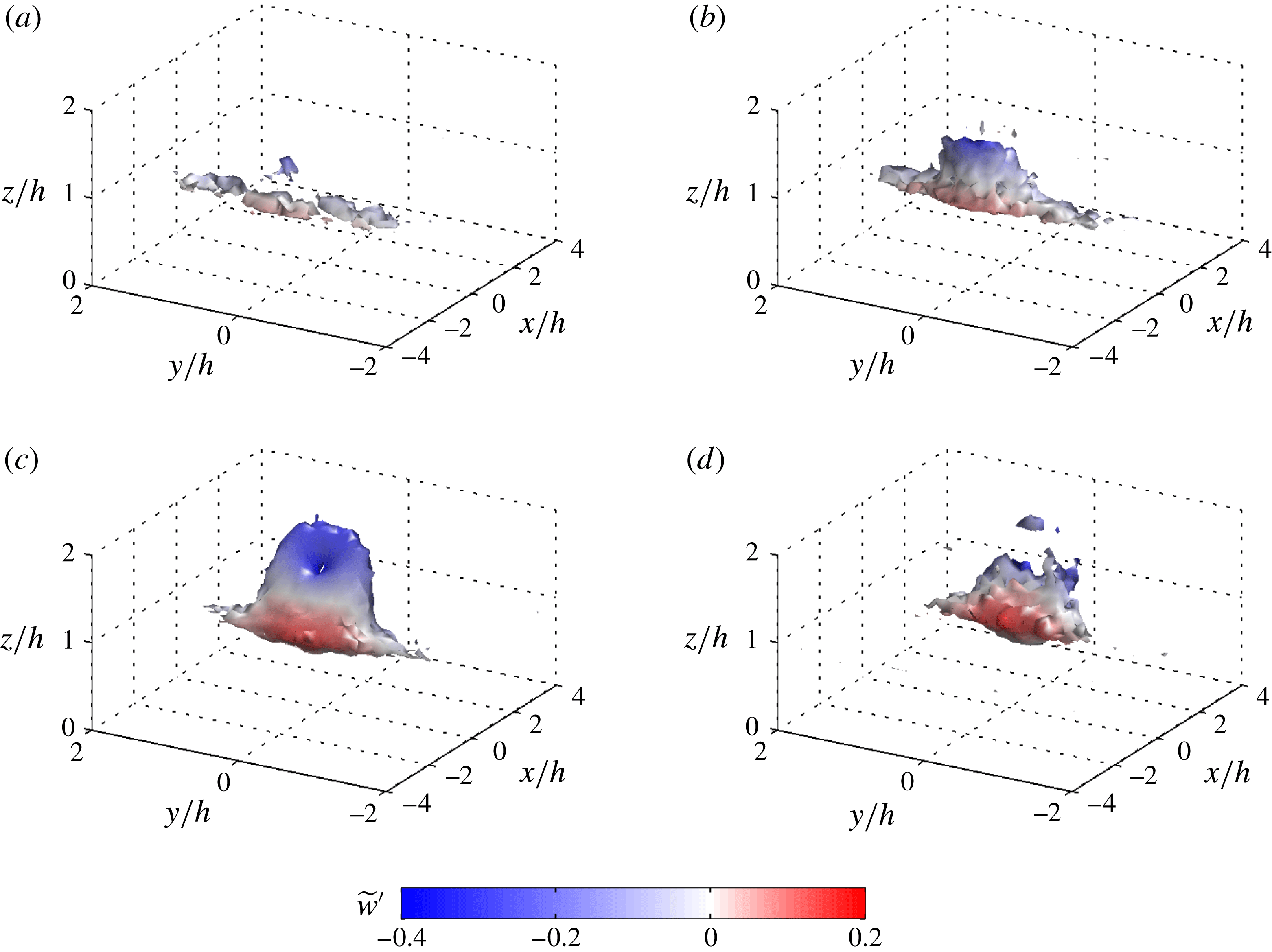
Figure 8 gives the time evolution of our composite structure based on a positive pressure perturbation (and mean shear included in
 ${\it\lambda}_{2}$
). The structure was obtained by following Finnigan et al. (Reference Finnigan, Shaw and Patton2009) and setting
 $c_{min}$
and
 $c_{max}$
respectively to 4.34 and 6.51, and
 $z_{T}/h=1.0$
. As noted by Finnigan et al. (Reference Finnigan, Shaw and Patton2009), varying the magnitude of
 $c$
within a reasonable range does not change the general shape of the structure. Rather we found it acted to add noise/distortion to the structure caused by not enough realizations (
 $c_{max}$
too high) or including too many weak structures (
 $c_{min}$
too low). An animation of the full time evolution of the composite structure can be found in supplementary movie 2.
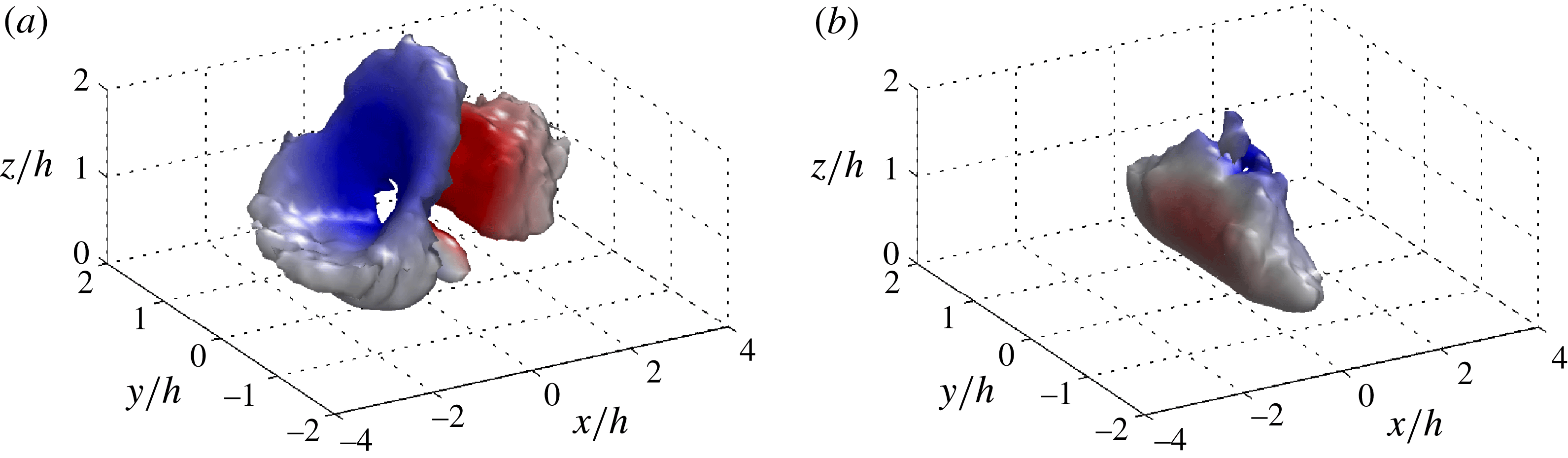
Composite eddy structure obtained by conditional sampling (
 $\mathscr{N}=40,592$
realizations) based on spikes in positive pressure perturbation at
 $z/h=1$
. The structure is visualized using isosurfaces of
 ${\it\lambda}_{2}$
at a value of
 $0.01\cdot \text{min}({\it\lambda}_{2})$
. The isosurfaces are coloured according to fluctuations in the filtered vertical velocity. (a)
 $tu^{\ast }/h=-0.176$
, (b)
 $tu^{\ast }/h=0$
, (c)
 $tu^{\ast }/h=0.176$
, (d)
 $tu^{\ast }/h=0.351$
. An animation of the full time evolution can be found in supplementary movie 2.

The composite structure emerges as a pair of predominantly spanwise structures located near the canopy top. The upwind structure primarily creates downward transport, while the downwind structure creates upward transport. The structure extends to about
 $\pm h$
in the spanwise direction before noise begins to break them up. As mentioned previously, we should not expect the composite rollers to extend the full width of the domain since irregularities will tend to disrupt their coherence far away from the trigger. This is especially true considering that the trigger location is between two structures. As time evolves, the structures remain at approximately the same spacing and shape and simply advect along the canopy top. At the time of the trigger, we find that the trigger location
 $\{x_{T},y_{T}\}$
is between the two structures, which is consistent with what was observed in the start-up flow.
Visual inspection indicates that the structures have a spacing of somewhere around
 $3h$
in the streamwise direction. Following Raupach et al. (Reference Raupach, Finnigan and Brunet1996), we estimated the theoretical mean streamwise structure spacing as
 ${\it\Lambda}_{x}=8.1L_{s}$
, where
 $L_{s}$
is the canopy-top shear length scale. Assuming the velocity profile approaches zero in the lower canopy,
 $L_{s}$
can be estimated as (Raupach et al.
Reference Raupach, Finnigan and Brunet1996)
 $$\begin{eqnarray}L_{s}=\frac{\overline{\langle u(h)\rangle }}{\partial \overline{\langle u\rangle }/\partial z\big|_{z=h}}.\end{eqnarray}$$
Using the profile in figure 7(a), we obtained a value of
 $L_{s}\approx 0.4h$
which gives
 ${\it\Lambda}_{x}\approx 3.25h$
. Thus, the composite structure roughly agrees with the expected structure spacing. This theoretical spacing will be further explored in § 5.2.1.
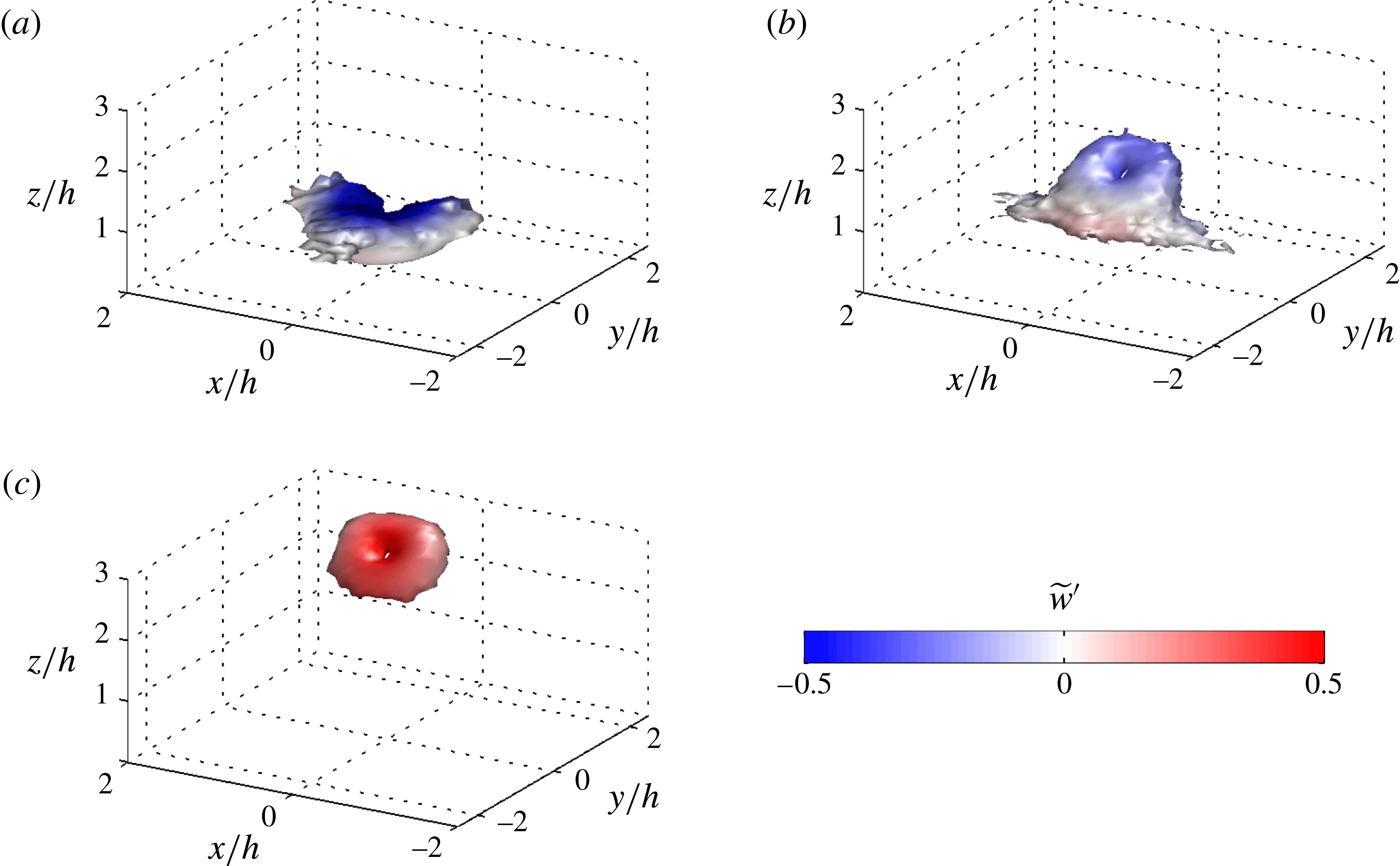
Our composite structure never has a strong three-dimensional shape for the duration of the composite evolution period that was examined. We can confirm that if we visualize the structure using the perturbation velocity/vorticity field (see figure 14
a), we indeed obtain a more three-dimensional structure that is similar to that reported by Finnigan et al. (Reference Finnigan, Shaw and Patton2009). In fact, this three-dimensional structure does not conflict with our conceptual model, and we do not contend that it is not a real feature of the flow. We find that the perturbation structure forms a ring vortex for most
 ${\it\lambda}_{2}^{\prime }$
isovalue choices. Finnigan et al. (Reference Finnigan, Shaw and Patton2009) also noted that certain isovalue choices showed a ring vortex. This perturbation structure agrees with the perturbation structure of a near-wall head-up hairpin shown by Kim & Moin (Reference Kim and Moin1986). It would appear that the three-dimensional structure is likely associated with a head-up hairpin as claimed by Finnigan et al. (Reference Finnigan, Shaw and Patton2009), but that removing the mean vorticity diminishes the surrounding two-dimensional structure.
We conclude that the three-dimensionality is largely associated with the perturbation vorticity field, but that a two-dimensional roller structure appears to dominate the pressure field and presumably the associated scalar microfronts/ramps. Again, this is not to say that the flow lacks substantial three-dimensionality. The composite structures themselves are a composite of many smaller three-dimensional vortices, which almost certainly undergo continuous localized interaction or pairing processes. The roller structure is also expected to have irregularities, including sinusoidal perturbations with wavelength of order
 ${\it\delta}$
resulting from mean streamwise streaks. We argue that it is an underlying quasi two-dimensional structure dominating the creation of observed pressure spikes and microfronts.
5.2.1. Flux contributions
Ultimately, our interest is in identifying the turbulent structures that dominate flow transport, that is the structures that give large contributions to mean turbulent stresses. One motivation for a conditional average based on spikes in pressure is that they usually coincide spatially with scalar microfronts, which are presumed to be associated with the generation of large turbulent fluxes. In § 3.2 we showed that in the start-up flow, pressure spikes did not coincide with large turbulent momentum fluxes, but rather they coincided with zero-crossings of momentum flux. The largest turbulent stresses were found on either side of the roller cores, which could be many canopy heights away from the pressure spike depending on mean structure spacing.
We seek to determine the correlation between positive spikes in pressure and turbulent fluxes of momentum and scalars in the fully-developed flow. This was quantified by summing the contribution to fluxes by regions of large pressure compared to their footprint area. As noted by Ganapathisubramani et al. (Reference Ganapathisubramani, Longmire and Marusic2003) and others, we should expect dominant structures to contribute a much larger percentage of the flux than the planar area they occupy.
We extracted two-dimensional boxes of instantaneous
 $u^{\prime }w^{\prime }=\tilde{u} ^{\prime }\tilde{w}^{\prime }+{\it\tau}_{13}$
and
 $w^{\prime }{\it\theta}^{\prime }=\tilde{w}^{\prime }\tilde{{\it\theta}}^{\prime }+q_{3}$
at
 $z=h$
. The boxes had length
 $r_{s}$
(streamwise) and width
 $r_{s}/2$
(spanwise), and were centred at local maxima in pressure satisfying the condition
 $\tilde{p}^{\prime }/u_{\ast }^{2}>c_{min}$
. Boxes were not allowed to overlap to avoid multiple counting of stress contributions. The stress fraction was defined as the sum of the flux within the boxes to the sum of the flux over the whole domain at
 $z=h$
. The footprint area fraction was defined as the ratio of the total area of all boxes to
 $L_{x}\times L_{y}$
. This was performed for instantaneous fields spaced in time at about
 $5\,u_{\ast }/h$
throughout the simulation.
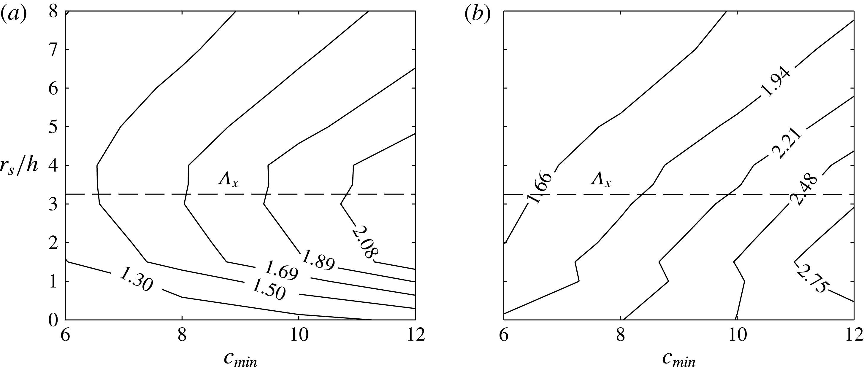
Ratio of contribution to turbulent fluxes to footprint area by regions of large positive pressure at
 $z=h$
for varying threshold
 $\tilde{p}^{\prime }/u_{\ast }^{2}>c_{min}$
. Boxes of instantaneous flux (a)
 $u^{\prime }w^{\prime }$
or (b)
 $w^{\prime }{\it\theta}^{\prime }$
were extracted around local maxima in pressure exceeding the threshold. Contours show their relative contributions to fluxes compared to the footprint area they occupied. The boxes had length
 $r_{s}$
in the streamwise direction and width
 $r_{s}/2$
in the spanwise direction. The horizontal dashed line denotes the estimated mean streamwise structure spacing
 ${\it\Lambda}_{x}$
using (5.1).

Figure 9 shows the ratio of the stress fraction to footprint area fraction (
 $\mathscr{R}$
) for varying values of
 $c_{min}$
and
 $r_{s}$
. For the chosen range of
 $c_{min}$
and
 $r_{s}$
, large regions of positive pressure gave relatively larger contributions to
 $u^{\prime }w^{\prime }$
than their footprint area, with
 $\mathscr{R}$
ranging from approximately 1.1 to 2.3. The lowest values of
 $\mathscr{R}$
were found when
 $r_{s}\rightarrow 0$
, which suggests that the largest mean Reynolds stresses are generally not located at the pressure spikes, which is an expected result. Rather, the largest values of
 $\mathscr{R}$
were found when
 $r_{s}$
was somewhere between
 $3h$
and
 $4h$
. As was discussed above, we used (5.1) to estimate the mean structure spacing and obtained a value of
 ${\it\Lambda}_{x}=3.25h$
, which is in agreement with the observed behaviour of
 $\mathscr{R}$
.
This result is significant for two primary reasons. First, it confirms the result found from the start-up flow that pressure spikes occur in the region between adjacent rollers which are located roughly
 ${\it\Lambda}_{x}/2$
in the upwind and downwind directions. Second, as argued by Finnigan et al. (Reference Finnigan, Shaw and Patton2009), there is some uncertainty in the proportionality constant value relating
 ${\it\Lambda}_{x}$
to
 $L_{s}$
, as the 8.1 value found by Raupach et al. (Reference Raupach, Finnigan and Brunet1996) is empirical. Our result corroborates the finding of Raupach et al. (Reference Raupach, Finnigan and Brunet1996). This result along with visual inspection of the structure spacing in our composite structure is evidence that
 ${\it\Lambda}_{x}=8.1L_{s}$
is a reasonable scaling relation for plant canopy flows.
Figure 9(b) gives the ratio of the
 $w^{\prime }{\it\theta}^{\prime }$
fraction to footprint area fraction. Overall, results suggest that pressure spikes give relatively larger contributions to scalar fluxes than momentum fluxes, with values of
 $\mathscr{R}$
ranging from about 1.4 to 3. It also appears that the spatial locations of pressure spikes and large vertical scalar fluxes are closely aligned, with maximum values of
 $\mathscr{R}$
occurring at less than
 ${\it\Lambda}_{x}/2$
. This results agrees qualitatively with conclusions from the start-up flow.
From the overall results of this section, we conclude that in both the start up and fully-developed flows, pressure maxima and corresponding scalar microfronts occur on average in the space between the dominant canopy-top structures. They are indicative of sharp local transitions between upward and downward transport. In and of themselves pressure maxima do not carry disproportionately large amounts of turbulent stress, rather the largest stresses are located a few canopy heights upstream and downstream of pressure maxima.
5.3. Reynolds-stress trigger
In this section, we created a composite averaging methodology to educe the composite structures associated with the generation of large Reynolds stresses. We recall from the start-up flow that the largest stress-generating structures (roller cores) coincided with regions of negative rather than positive pressure. It is reasonable then to consider a conditional averaging trigger based on pressure minima (cf. Hunt et al. Reference Hunt, Wray and Moin1988; Jeong & Hussein Reference Jeong and Hussein1995). However, in the fully developed very high Reynolds number case, the rollers are not traditional vortex tubes but rather a conglomeration of smaller vortices exhibiting rotational motion. Thus, we should expect the rollers to be associated with negative pressure on average, but not necessarily instantaneous pressure minima.
To directly seek out the dominant structures contributing to Reynolds stresses, we formulated a conditional averaging methodology based on a trigger of local maxima in
 $-u^{\prime }w^{\prime }=-(\tilde{u} ^{\prime }\tilde{w}^{\prime }+{\it\tau}_{13})$
. As also noted by Ganapathisubramani et al. (Reference Ganapathisubramani, Longmire and Marusic2003), one advantage of this trigger is that it does not bias toward either sweeps or ejections, since both can contribute to
 $-u^{\prime }w^{\prime }$
. The methodology we used is the same as described in § 5.2 except that a composite-averaging event is triggered based on local minima of regions where
 $c_{min}u_{\ast }^{2}(z_{T})<u^{\prime }w^{\prime }<c_{max}u_{\ast }^{2}(z_{T})$
, where here
 $u_{\ast }^{2}(z_{T})$
is (minus) the mean Reynolds stress at the trigger height rather than the canopy height. Threshold values of
 $c_{min}$
and
 $c_{max}$
were respectively given values of
 $-18$
and
 $-14$
.
Time evolution of composite eddy structure obtained by conditional sampling (
 $\mathscr{N}=25,345$
realizations) based on local minima of
 $u^{\prime }w^{\prime }$
at
 $z_{T}/h=1.5$
. The structure is visualized using isosurfaces of
 ${\it\lambda}_{2}$
at a value of
 $0.01\cdot \text{min}({\it\lambda}_{2})$
. The isosurfaces are coloured according to fluctuations in the filtered vertical velocity. (a)
 $tu^{\ast }/h=-0.527$
, (b)
 $tu^{\ast }/h=-0.351$
, (c)
 $tu^{\ast }/h=0$
, (d)
 $tu^{\ast }/h=0.439$
. An animation of the full time evolution can be found in supplementary movie 3.

Composite eddy structure obtained by conditional sampling based on local minima of
 $u^{\prime }w^{\prime }$
at varying trigger heights of (a)
 $z_{T}/h=0.75$
, (b)
 $z_{T}/h=1.5$
, (c)
 $z_{T}/h=3.0$
. The structure is visualized using isosurfaces of
 ${\it\lambda}_{2}$
at a value of
 $0.01\cdot \text{min}({\it\lambda}_{2})$
. The isosurfaces are coloured according to fluctuations in the filtered vertical velocity.

The time evolution of the composite structure is shown in figure 10. An animation of the full time evolution can be found in supplementary movie 3. The composite structure emerges as a predominantly spanwise vortex structure that is at least
 $4h$
wide in the
 $y$
direction. The structure has the expected sense of rotation for a spanwise roller structure, as indicated by patters in
 $\tilde{w}^{\prime }$
. This predominantly spanwise structure supports the conceptual model Stages (a)–(b), and our previous hypothesis that the flow is dominated by an underlying two-dimensional structure. It is interesting to note that whether
 ${\it\lambda}_{2}$
or
 ${\it\lambda}_{2}^{\prime }$
is used to visualize the structure (see figure 14
b), a two-dimensional structure is still present. This is likely due to the fact that when the stress trigger is used, the structure is located at the trigger location. We can also confirm that if perturbation velocity vectors are used to visualize the structure (not shown), a two-dimensional structure is clearly present that is at least
 $4h$
wide in the spanwise. It is likely that the closer the structure of interest is located to the trigger location, the better defined it will be. The further the structure from the trigger location, the more it is liable to be eliminated by removing mean vorticity, and by composite averaging in general.
As time progresses, a hairpin-like structure forms above the spanwise structure inclined at approximately
 $45^{\circ }$
. This supports conceptual model stages (c)–(d). Away from the hairpin, the still predominantly spanwise portion of the structure generates sweep events, particularly on its downwind side. We do not observe any clear formation of a head-down hairpin structure, although one could argue that a ‘bulge’ exists where head-down structures would be located. Note also that the base of the structure is centred about
 $x=0$
at
 $t=0$
, in contrast to the structure in figure 8 where there was no structure in the immediate vicinity of
 $x=0$
at
 $t=0$
. This means that the actual structure is centred at the trigger location rather than surrounding it. As time progresses further, the head of the upper hairpin-like structure separates from the predominantly spanwise structure at the canopy top, supporting the ‘recycling’ stage of the conceptual model. Overall, the evolution of the composite structure is similar to what was observed in the start-up flow, and supports the conceptual model presented in § 4. It is impossible to fully support conceptual model Stage (b) with the composite structures, since their nature is to aggregate smaller structures. However, vortex breakdown is inevitable, and it is entirely inconceivable to imagine that a well-defined spanwise vortex tube exists given the extremely high Reynolds number and the frequently reported existence of an approximately
 $k^{-5/3}$
kinetic energy spectrum near the canopy (Finnigan Reference Finnigan2000; Bailey & Stoll Reference Bailey and Stoll2013).
The selected height of the trigger
 $z_{T}$
had an influence on the resulting composite structure and suggested that different structures dominate Reynolds stresses at different heights. Figure 11 shows the variation of the composite structure with
 $z_{T}/h=0.75$
, 1.5, and 3.0. At a trigger height of
 $0.75h$
, the composite structure is predominantly spanwise, and resembles the composite structure in figure 10 at times well before and after the triggering event. The structure has a slight bend around the trigger location, but as will be shown in the next section, this is because it likely resides in a low-speed streak. For a trigger height just above the canopy, we still obtain the predominantly spanwise structure, but an additional structure resembling that of a head-up hairpin emerges. As the trigger height is increased to several canopy heights, the resulting structure resembles the head of a head-up hairpin, although this is speculative since the details of the legs are not visible. This could be a deficiency of the composite-averaging method, which tends to lose structure detail far away from the trigger location. Qualitatively, this trend with varying
 $z_{T}$
agrees with the conceptual model presented in § 4.
5.4. Location of trigger events
If we examine temporally-averaged flow fields, we find that as in the start-up flow (figure 4
d) a streaked pattern emerges in many flow variables. Figure 12 shows temporally-averaged fields of streamwise velocity fluctuation
 $\overline{u^{\prime }}$
(figure 12
a), pressure fluctuation
 $\overline{p^{\prime }}$
(figure 12
b) and scalar fluctuation
 $\overline{{\it\theta}^{\prime }}$
(figure 12
c) at the canopy top.
 $\overline{u^{\prime }}$
has pronounced sinusoidal streaks in the streamwise direction, corresponding to weak streamwise vortices.
Temporally averaged
 $x{-}y$
slices at
 $z=h$
of (a) streamwise velocity perturbation, (b) pressure perturbation, and (c) scalar perturbation. Spatial coordinates are normalized by the boundary-layer height
 ${\it\delta}=L_{z}$
. The right column shows the probability density function of conditional averaging trigger event spanwise locations for pressure trigger (squares) and Reynolds-stress trigger (circles). Note that the same plot is repeated for comparison with each
 $x$
–
 $y$
slice.

We find that the spanwise wavelength of our mean streamwise structures scales with
 $L_{z}$
, or equivalently the boundary-layer height
 ${\it\delta}$
. This would suggest that secondary instability in the overlying boundary results in in-phase displacements of primarily spanwise structures even near the canopy. The patterns in
 $\overline{u^{\prime }}$
and
 $\overline{{\it\theta}^{\prime }}$
suggest that certain streamwise regions of the flow favour upward transport.
To investigate the relationship with our detected coherent structures and mean streamwise structures, we created a probability density function (PDF) of trigger locations. This PDF is plotted alongside the temporally-averaged fields in figure 12(a–c). We found that most of the composite trigger events corresponded to mean streaks of negative
 $\overline{u^{\prime }}$
, positive
 $\overline{p^{\prime }}$
and positive
 $\overline{{\it\theta}^{\prime }}$
. Intuitively, it makes sense that since our composite-averaging methodology seeks out large Reynolds-stress events, most trigger events would happen in regions of low-momentum fluid which presumably favour the generation of head-up hairpin vortex packets. Not surprisingly, the resulting composite structure was associated with a head-up hairpin structure. We suspect that any conditional-sampling methodology seeking to capture large variance or flux events will be liable to bias toward these regions of low-momentum fluid and corresponding packets of hairpin vortices. Hence, they are likely to return a structure with some degree of three-dimensionality. This is exemplified by our Reynolds-stress trigger, and previously used methodologies based on empirical orthogonal function (EOF) decompositions (e.g. Finnigan & Shaw Reference Finnigan and Shaw2000). Care should be taken when using perturbation fields to visualize composite-averaged fields based on a point of large pressure, stress, variance, etc., because the perturbation field will tend to create a three-dimensional perturbation structure that surrounds the trigger point.
This result agrees with the start-up flow where we found that the tallest head-up hairpin structures tended to form along streamwise transects associated with low-momentum fluid. This also offers evidence to support our conceptual model, where we claimed that head-up hairpin formation is most commonly in phase between adjacent rollers.
6. Summary
This study sought to identify the coherent turbulent structures that dominate fluxes in the roughness sublayer, and characterize their evolution. To examine this problem, we used the case of a horizontally homogeneous body of drag elements sitting atop the lower boundary (e.g. a plant canopy). In this paper, we proposed a new conceptual model that attempts to address some of the remaining questions from previous work. Criteria for the evaluation of the conceptual model were suggested, which are that it must at a minimum explain the following features observed in canopy flows:
-
(1) An overall high degree of coherence and mixing, with dominant turbulent length scales of the order of the canopy height.
-
(2) Dominant turbulent length scales near the canopy top are a linear function of the canopy-top shear length scale.
-
(3) Near the canopy, sweep events dominate mean turbulent fluxes, although ejection events are more frequent. This smoothly transitions to the opposite behaviour in the overlying ISL.
-
(4) Periodic patterns of relatively long-duration upward transport (ejections) followed by strong and abrupt downward-transport events (sweeps) leading to high local streamwise gradients and characteristic ‘ramp’ structures.
-
(5) The presence of weak mean streamwise vorticity in the streamwise direction resulting in alternating mean streamwise streaks of high/low momentum.
This problem was examined in two stages. First, LES was used to simulate start-up flow in which turbulent motions were observed as they emerged out of an initially two-dimensional, laminar flow field. Since the full range of turbulent length scales had not yet developed, this allowed for the visualization of instantaneous coherent structures and initially removed the effects of three-dimensionality. The structures that dominate fully-developed flows were of ultimate interest, and therefore composite-averaging techniques were also used to extract ‘characteristic’ realizations of coherent structures from quasi-steady simulations. Both the start up and fully-developed visualization techniques revealed a similar chain of events associated with the evolution of coherent structures, which can be summarized by our proposed conceptual model.
We found that fluxes near the canopy are dominated by an underlying spanwise roller structure that is predominantly two-dimensional, which qualitatively satisfies conceptual criterion (1) and (2). This structure is similar to that of a planar mixing layer, as was first detailed by Raupach et al. (Reference Raupach, Finnigan and Brunet1996). Because the Reynolds number is large in real canopy flows, the two-dimensional roller structures are not a coherent vortex tube as would traditionally be associated with a vortex in laminar flow. Rather, they are larger-scale vortical motions that transport smaller three-dimensional vortices in a net circular motion. Smaller-scale vortices continually undergo localized interaction processes, however the fundamental conclusion of this paper is that, as in a mixing layer, these interactions do not act to destroy the larger-scale two-dimensional structures. These larger-scale structures are not likely to be exactly two-dimensional as they contain random irregularities as well as regular perturbations associated with mean spanwise heterogeneity. It is because of this fact that they are not as readily detected in correlation or conditional sampling analyses.
The observed streamwise roller spacing confirmed the scaling of Raupach et al. (Reference Raupach, Finnigan and Brunet1996). We also used the start-up flow to show how a two-dimensional structure, combined with blocking by the canopy and wall, leads to a dominance of sweep events in Reynolds stresses, but more frequent ejection events overall (conceptual criteria (3)). One of the most important distinctions between mixing-layer flow and canopy flow is momentum absorption by the canopy or lower wall, which creates vertical asymmetry. We found that the roller vortex core is displaced above the canopy top, which explains reported behaviour of convective velocity scales.
Mean shear and localized vortex sheets sustain the production of an often self-similar fine-scale vortex structure. As they evolve, these fine-scale vortices are continually stretched and strained resulting in highly three-dimensional fine-scale structure. Smaller vortices that are stretched and strained downward are inhibited to some degree by the low-flux canopy. Vortices that stretch upward often form hairpin structures as they are relatively unbounded from above. These structures evolve to form the hairpin structures that have been found to populate the ISL (Adrian Reference Adrian, Venditti, Best, Church and Hardy2013). This process can repeat indefinitely as rollers generate smaller vortices, which continually stretch upward into hairpins, then break down and become decorrelated with the canopy-top structures. This does not contradict Townsend’s attached-eddy hypothesis, since in our conceptual model the near-canopy and ISL structures evolve together.
The start-up flow also demonstrated how a two-dimensional structure could create the observed scalar microfront or ramp patterns, thus satisfying criteria (4). Strong microfronts are created in the ‘slip’ region between adjacent roller structures, where there exists sharp local transitions between upward and downward transport. This is similar in principle to how microfronts are generated in other shear flows. However, in the roughness sublayer, microfronts are especially strong due the elevated maximum in shear which sustains them. Microfronts are also asymmetrical (ramp-like) due to blocking by the lower boundary.
The dominant two-dimensional structure is in contrast to the conceptual model of Finnigan et al. (Reference Finnigan, Shaw and Patton2009), which does not depict a sustained two-dimensional structure. Our model could also be interpreted as contradicting two-point correlation measurements, which have found spanwise correlation length scales of around
 $h$
or less (Shaw et al.
Reference Shaw, Brunet, Finnigan and Raupach1995). While we find that the flow is indeed highly three-dimensional and populated with numerous hairpin-like structures that continually interact, we found strong evidence that an underlying two-dimensional roller structure dominates turbulent fluxes. The plausibility of this argument was established by the two-dimensional start-up flow, which produced the characteristic scalar ramp structures and a vertical sweep-ejection structure commonly observed in experiments. More direct evidence was given using composite averages based on spikes in pressure and Reynolds stress, which both revealed a predominately two-dimensional roller structure. Based on this evidence, our fundamental conclusion was that, as in a mixing layer, a global instability mechanism creates a sustained two-dimensional structure that dominates the flow, rather than the three-dimensional structure resulting from local instability as claimed by Finnigan et al. (Reference Finnigan, Shaw and Patton2009). We argued that the composite averages of Finnigan et al. (Reference Finnigan, Shaw and Patton2009) likely identified only a three-dimensional structure because their conditional-averaging trigger only targeted the space between structures, and then visualized structures using only the perturbation velocity field. The low spanwise correlation scales found in previous work is likely due to spanwise irregularities or meandering of the predominantly two-dimensional structures, which is supported by previous work which has found that slight irregularities can severely reduce spanwise correlation measurements. There is no reason to believe that many of the localized three-dimensional vortex interaction processes described by Finnigan et al. (Reference Finnigan, Shaw and Patton2009) are not also present. Rather, it is argued that a dominant larger-scale structure exists, but is not as readily detected because of such irregularities.
Future work regarding coherent structure detection should focus on developing methods that can detect and visualize structures instantaneously in very high Reynolds number cases. The composite aggregation of structures introduces substantial uncertainty, whether it be through composite averaging, correlation analysis, etc., because larger-scale structures often become averaged out. There is always the risk when averaging that important structures will be missed, or spurious structures will be introduced.
Unanswered questions specifically regarding the structure of canopy flows still remain. Future work on this subject should involve investigating how varying canopy architecture influences the above processes. We know that varying overall canopy density changes canopy-top shear, which in turn determines the spacing between adjacent roller structures (Raupach et al. Reference Raupach, Finnigan and Brunet1996; Brunet & Irvine Reference Brunet and Irvine2000). At some critically low value of canopy density, the roller-like structures must become unimportant as the flow transitions to that of a boundary layer where shear at the wall dominates. Canopy heterogeneity is known to have an impact on the transport of momentum and scalars (Bailey & Stoll Reference Bailey and Stoll2013; Bailey et al. Reference Bailey, Stoll, Pardyjak and Mahaffee2014), and is also likely to influence turbulent structure development. It is likely that the presence of heterogeneity may cause the development of the mixing-layer-like structures to be more like that of a spatially-developing mixing layer in the wake of individual canopy elements.
Acknowledgements
The authors wish to thank Dr E. Pardyjak for many useful discussions regarding this work. This research was supported by US National Science Foundation (NSF) grants EPS 1208732, and AGS 1255662. Any opinions, findings, and conclusions or recommendations expressed are those of the authors and do not necessarily reflect the views of the National Science Foundation. We acknowledge high-performance computing support from Yellowstone (ark:/85065/d7wd3xhc) provided by NCAR’s Computational and Information Systems Laboratory, sponsored by the NSF. An allocation of computer time from the Center for High Performance Computing at the University of Utah is also gratefully acknowledged.
Supplementary movies
Supplementary movies are available at http://dx.doi.org/10.1017/jfm.2015.749.
Appendix. Structure associated with the perturbation vorticity field
We evaluated the implications of visualizing flow structures using a
 ${\it\lambda}_{2}$
with mean gradients removed, as was done by Finnigan et al. (Reference Finnigan, Shaw and Patton2009). We define the ‘perturbation’
 ${\it\lambda}_{2}$
(denoted by the symbol
 ${\it\lambda}_{2}^{\prime }$
) as the second largest eigenvalue of the tensor
 $(\unicode[STIX]{x1D61A}_{ij}^{\prime })^{2}+({\it\Omega}_{ij}^{\prime })^{2}$
, with
 $\unicode[STIX]{x1D61A}_{ij}^{\prime }=((\partial u_{i}^{\prime }/\partial x_{j})+(\partial u_{j}^{\prime }/\partial x_{i}))/2$
and
 ${\it\Omega}_{ij}^{\prime }=((\partial u_{i}^{\prime }/\partial x_{j})-(\partial u_{j}^{\prime }/\partial x_{i}))/2$
. We can loosely interpret structures identified by
 ${\it\lambda}_{2}^{\prime }$
as structures corresponding to the perturbation vorticity.
Same as figure 4, except that structures are visualized using isosurfaces of
 ${\it\lambda}_{2}^{\prime }$
, which is
 ${\it\lambda}_{2}$
based on a perturbation velocity field.

As an illustrative example, we first consider recreating figure 4 with structures visualized using
 ${\it\lambda}_{2}^{\prime }$
rather than
 ${\it\lambda}_{2}$
(figure 13). For early development of the start-up simulation, the flow is essentially two-dimensional, and is dominated by a train of three spanwise roller structures. In addition to figure 4(a), this can be confirmed by plotting isocontours of spanwise vorticity
 ${\it\omega}_{2}$
as in figure 2(a). However, using isosurfaces of
 ${\it\lambda}_{2}^{\prime }$
depicts quite a different configuration. Removing the mean velocity gradient from
 ${\it\lambda}_{2}$
splits each of the rollers into two and we are left with perturbations from the roller vortex structure. Based on figure 13(a), one could be led to believe that the flow is dominated by six pairs of spanwise rollers, with an upper roller situated above and downstream of a lower roller. It is clear that this is not a dominant feature of the flow, but rather that it arose after removing mean shear from the structures. For later time evolution when the flow is still predominantly two-dimensional but with some pronounced three-dimensionality (figure 13
b), the primary two-dimensional structure remains intact when
 ${\it\lambda}_{2}^{\prime }$
is used, but an additional spanwise structure arises in the region between two adjacent rollers. When the flow is highly three-dimensional (figure 14
c),
 ${\it\lambda}_{2}$
and
 ${\it\lambda}_{2}^{\prime }$
provide similar visualizations, since at this point there is no well-defined net roller vortex structure.
Next we consider composite structures when visualized using
 ${\it\lambda}_{2}^{\prime }$
. Figure 14 gives the composite structure for a trigger based on (a) positive spikes in pressure, and (b) large negative Reynolds stress, visualized using isosurfaces of
 ${\it\lambda}_{2}^{\prime }$
. Here, removing the mean velocity gradient removes much of the predominantly spanwise nature of the structure, to reveal instead a highly three-dimensional structure. However, we feel that the perturbation structures still agree with our conceptual model, if we are careful in considering that the mean (spanwise) vorticity has been removed. The composite structure based on a pressure trigger (figure 14
a) shows a looped vortex that is flat on the bottom side. This is consistent with the perturbation vortex structure associated with the head-up hairpin structure in a boundary shown by Kim & Moin (Reference Kim and Moin1986). Note that the structure reported in Finnigan et al. (Reference Finnigan, Shaw and Patton2009) does not connect on the upper side to create a loop, and they therefore interpret this as a head-down hairpin. They do however note that for certain
 ${\it\lambda}_{2}^{\prime }$
isovalues they did observe a looped structure, although they are not specific as to the range of
 ${\it\lambda}_{2}^{\prime }$
isovalues that produced a closed loop. We found that it took somewhat extreme
 ${\it\lambda}_{2}^{\prime }$
isovalues to make the loop disappear, and that most
 ${\it\lambda}_{2}^{\prime }$
isovalue choices produced a looped structure that looks like that of the perturbation vorticity field of a head-up hairpin reported by Kim & Moin (Reference Kim and Moin1986).
Linking this structure back to the structure associated with total vorticity (figure 8), we find that the head-up hairpin emanates from the upwind roller structure. If we visualize the time evolution of the composite perturbation structure (not shown) we find that the head-up hairpin is continually stretched and strained toward the next adjacent roller. Since the head-up hairpin moves toward the adjacent roller, Finnigan et al. (Reference Finnigan, Shaw and Patton2009) interpreted this as ‘pairing’, although the underlying spanwise roller structure never actually pairs. When we add in the mean vorticity as in figure 8, the head-up hairpin structure is not readily visible. This indicates that it is the predominantly two-dimensional structure that dominates the creation of large pressure spikes (and presumably microfronts), but there is also an associated three-dimensional perturbation structure that is dominated by head-up hairpins.
Figure 14(b) shows that both
 ${\it\lambda}_{2}$
and
 ${\it\lambda}_{2}^{\prime }$
identify a spanwise roller vortex when the Reynolds-stress trigger is used.