



1. Introduction
Within the transonic flight regime of aircraft, self-sustained shock oscillations occur once the freestream Mach number and angle of attack exceed critical parameter combinations. This complex aerodynamic phenomenon, induced shock-wave/boundary-layer interaction, is termed shock buffet (also referred to as transonic buffet). These oscillations can lead to significant fluctuations in aerodynamic forces, which reduce flight handling qualities and limit the flight envelope (Giannelis et al. Reference Giannelis, Vio and Levinski2017). Identifying transonic shock buffet onset boundaries typically relies on quasi-steady or steady freestream tests. In realistic flight scenarios, typical operational manoeuvres, such as wind-up turns and pull-up motions, involve continuous angle-of-attack variations at finite pitch rates. Numerical investigations of continuous pitching motion confirm that elevated pitch rates delay the initiation of discernable oscillations (Crouch et al. Reference Crouch, Ahrabi and Kamenetskiy2024). Such buffet delay induces measurable discrepancies in buffet onset characteristics between quasi-steady evaluations and continuous sweep conditions. Accordingly, dynamic buffet onset boundaries that account for continuous pitching effects are essential for reliable aerodynamic assessment of practical transonic manoeuvre conditions.
Extensive experimental and numerical investigations have been carried out to reveal the underlying physics of transonic buffet (Hilton & Fowler Reference Hilton and Fowler1947; Barakos & Drikakis Reference Barakos and Drikakis2000; Iovnovich & Raveh Reference Iovnovich and Raveh2015; Dandois Reference Dandois2016; Masini et al. Reference Masini, Timme and Peace2020). An early bubble bursting model for transonic buffet was presented by Pearcey (Reference Pearcey1958) and Pearcey & Holder (Reference Pearcey and Holder1962), associating buffet onset with trailing edge separation bubble bursting. Drawing upon later contradictory observations (Crouch et al. Reference Crouch, Garbaruk, Magidov and Travin2009; Nitzsche Reference Nitzsche2009; Sartor et al. Reference Sartor, Mettot and Sipp2015), bubble bursting is now widely discounted as a potential mechanism driver for shock buffet onset. For two-dimensional aerofoils, Lee (Reference Lee1990) proposed an acoustic wave-propagation feedback model for Tijdeman type A shock motions, where downstream-travelling pressure waves from the shock interact with upstream-propagating acoustic disturbances generated at the trailing edge, forming a closed feedback loop that sustains periodic shock oscillations. This receives support from certain experimental and numerical investigations, though conflicting results are also reported in other studies (Garnier & Deck Reference Garnier and Deck2010; Hartmann et al. Reference Hartmann, Feldhusen and Schröder2013a ; Feldhusen-Hoffmann et al. Reference Feldhusen-Hoffmann, Lagemann, Loosen, Meysonnat, Klaas and Schröder2021; Moise et al. Reference Moise, Zauner and Sandham2022). Rooted in stability theory, the work of Crouch et al. (Reference Crouch, Garbaruk and Magidov2007, Reference Crouch, Garbaruk, Magidov and Travin2009) demonstrated that transonic buffet on aerofoils originates from a supercritical Hopf bifurcation of the steady flow, a finding further supported by subsequent studies (Kuz’min Reference Kuz’min2009; Sartor et al. Reference Sartor, Mettot and Sipp2015; Paladini et al. Reference Paladini, Marquet, Sipp, Robinet and Dandois2019). Above critical conditions, a globally unstable flow mode induces phase-locked oscillations between the shock and separated boundary layer. Recently, global stability analyses have been performed for practical finite-wing aircraft (Timme & Thormann Reference Timme and Thormann2016; Timme Reference Timme2020; Sansica & Hashimoto Reference Sansica and Hashimoto2023), for which shock buffet is also linked to a globally unstable mode.
Building on foregoing investigations into the underlying mechanisms of shock buffet, this phenomenon exhibits intrinsic nonlinear evolutionary characteristics. This allows the associated flow field behaviours to be grouped into two distinct regimes. Weakly nonlinear buffet emerges near the supercritical Hopf bifurcation in the near-critical regime beyond the buffet onset boundary, where linear growth rates and disturbance amplitudes remain small. As demonstrated by Crouch et al. (Reference Crouch, Ahrabi and Kamenetskiy2024), such near-critical finite-amplitude transonic buffet oscillations can be accurately captured by weakly nonlinear analysis via the Landau equation. As the angle of attack increases beyond the buffet onset, the shock-wave/boundary-layer coupling intensifies, and the flow evolves into a strongly nonlinear regime. Within this regime, aerodynamic resonance emerges under shock-induced separation (Davis & Malcolm Reference Davis and Malcolm1980; Despré et al. Reference Despré, Caruana, Mignosi, Reberga, Corrège, Gassot, Le Balleur and Girodroux-Lavigne2000), while frequency lock-in occurs either via forced excitation near the natural buffet frequency with sufficient amplitudes (Raveh Reference Raveh2009; Iovnovich & Raveh Reference Iovnovich and Raveh2012; Hartmann et al. Reference Hartmann, Klaas and Schröder2013b ) or self-induced fluid–structure interaction covering fluid-mode, veering and structural-mode regimes without an amplitude threshold (Gao et al. Reference Gao, Zhang, Li, Liu, Quan, Ye and Jiang2017; Korthäuer et al. Reference Korthäuer, Accorinti, Scharnowski and Kähler2023). Apart from local periodic oscillations, flow lag and lead effects linked to separation and reattachment further create hysteresis loops of aerodynamic coefficients. Multi-valued aerodynamic responses emerge along distinct ascending and descending angle-of-attack variation branches, as reported for low Reynolds number wake hysteresis and transonic shock buffet flows (Rahman et al. Reference Rahman, Hasan and Labib2015; Marquet et al. Reference Marquet, Leontini, Zhao and Thompson2022; Masdari et al. Reference Masdari, Zeinalzadeh, Abdi and Soltani2022). Whereas resonance and frequency lock-in represent local shock fluctuations within the buffet regime, hysteresis acts as a global flow evolution feature differentiating static and dynamic buffet boundaries.
To investigate such buffet boundary hysteresis, a series of computational studies has been carried out over the past decades. Nitzsche (Reference Nitzsche2009) conducted numerical investigations on a supercritical aerofoil using the unsteady Reynolds-averaged Navier–Stokes (URANS) method, aiming to explore the fixed-point stability and small-perturbation response of the steady flow field prior to buffet onset. By performing angle-of-attack sweeps in both ascending and descending directions, this study identified buffet hysteresis within the range
 $4.5^{\circ }{-} 5.5^{\circ }$
, which arises from the coexistence of a stable steady flow solution and a shock buffet limit cycle oscillation alongside. Murray et al. (Reference Murray, Giannellis and Vio2020) developed a cusp-catastrophe model to characterise the buffet hysteresis boundaries in ascending and descending angle-of-attack sweeps, and demonstrated that the buffet hysteresis envelope is highly nonlinear with Mach number, and exhibits clear path dependence during angle-of-attack sweeps. Focusing on the supercritical Hopf bifurcation regime near buffet onset, Crouch et al. (Reference Crouch, Ahrabi and Kamenetskiy2024) applied global stability and weakly nonlinear theory with the Landau equation to model buffet amplitude evolution on the OAT15A aerofoil, allowing accurate prediction of the lift oscillation envelope. They demonstrated that increasing the pitch rate only delays buffet onset without affecting the limiting oscillation amplitude. While existing studies have recognised path- and rate-dependent hysteresis in transonic buffet during dynamic angle-of-attack sweeps, effective prediction methods for buffet boundaries under variable-rate and variable-path manoeuvres remain lacking.
In recent years, a variety of data-driven reduced-order and dynamic analysis approaches have been developed for buffet research and analysis. Modal decomposition techniques based on flow field snapshots, including proper orthogonal decomposition (Hall et al. Reference Hall, Thomas and Dowell2000; Iuliano & Quagliarella Reference Iuliano and Quagliarella2013) and dynamic mode decomposition (DMD) (Rowley et al. Reference Rowley, Mezić, Bagheri, Schlatter and Henningson2009; Kou & Zhang Reference Kou and Zhang2017) as well as other related schemes (Dias et al. Reference Dias, Budišić, Piperni and Helenbrook2024; Zamani Ashtiani & Fukami Reference Zamani Ashtiani and Fukami2026), are capable of extracting dominant coherent structures from complex flows. Global stability analysis (Crouch et al. Reference Crouch, Garbaruk, Magidov and Travin2009; Timme Reference Timme2020) and resolvent analysis (Iwatani et al. Reference Iwatani, Asada, Yeh, Taira and Kawai2023) linearise the governing equations around steady base flows, enabling identification of the Hopf bifurcation and quantification of energy amplification for shock oscillations. Nevertheless, these analyses are typically limited to discrete fixed operating conditions, assessing buffet flow characteristics on a point-by-point basis. Unlike full-field decomposition methods, linear system identification techniques such as the autoregressive with exogenous input (ARX) model (Zhang et al. Reference Zhang, Li, Ye and Jiang2015) and the eigensystem realisation algorithm (Juang & Pappa Reference Juang and Pappa1985; Kim Reference Kim2005) recover low-order dynamic models directly from aerodynamic load time histories. The linear ARX framework has been applied to small-disturbance stability analysis of transonic buffet (Gao et al. Reference Gao, Zhang, Li, Liu, Quan, Ye and Jiang2017), and its periodic-coefficient extension has been employed for linear time-periodic unsteady aerodynamic modelling of rotary wings (Quero Reference Quero2024). However, these methods struggle to cope with large-amplitude and aperiodic excitations. To effectively characterise the strong nonlinear behaviours of transonic buffet flows, Volterra series (Balajewicz & Dowell Reference Balajewicz and Dowell2012), sparse identification of nonlinear dynamics (SINDy) (Sansica et al. Reference Sansica, Loiseau, Kanamori, Hashimoto and Robinet2022) and deep learning approaches (Kou & Zhang Reference Kou and Zhang2021; Fukami et al. Reference Fukami, Iwatani, Maejima, Asada and Kawai2025; Candon et al. Reference Candon, Marzocca and Dowell2026) have been widely employed for nonlinear dynamical flow modelling and low-dimensional latent representations. While Volterra series and SINDy yield explicit nonlinear dynamic equations, the functional form of the Volterra series and the reliance of SINDy on a pre-specified candidate library hinder analytical characterisation of complex unsteady flow dynamics. Deep learning approaches serve as surrogate models without an explicit dynamical formulation, precluding direct stability assessment.
Owing to flow hysteresis, the instantaneous shock structure and flow separation depend not only on the current angle of attack but also on its variation history. Rapid angle-of-attack ramping shortens the growth period of flow instabilities and thereby delays the onset of shock oscillation. Most existing approaches either characterise buffet at discrete fixed operating conditions point-by-point, or rely on fixed-parameter models that struggle with large-amplitude aperiodic excitations. Against this background, this paper develops a time-varying ARX (TV-ARX) model for the dynamic identification of transonic buffet under continuous angle-of-attack sweeps. Unlike stationary fixed-parameter ARX counterparts, the present framework constructs sequential linear input–output mappings for unsteady buffet systems. Drawing on historical input–output information within its regression structure, it employs the variable-forgetting-factor recursive least squares (VFF-RLS) scheme for adaptive coefficient updates, thereby capturing the time-varying dynamics associated with flow hysteresis. With these adaptively updated coefficients, the TV-ARX model tracks the time-varying state matrix to characterise the evolution of system stability, and thus provides an estimate of the practical shock buffet onset boundary under continuous pitching motion.
The paper is organised as follows. Section 2 presents the general process of time-varying modelling, specific numerical simulation methods, and the TV-ARX model with a tailored adaptive scheme. Section 3 introduces the stability criteria derived from eigenvalue analysis, alongside validation tests using a second-order oscillator with time-varying damping. Section 4 investigates the evolution of flow stability characteristics from linear to nonlinear buffet under fixed flow conditions. Section 5 is dedicated to buffet boundary prediction for ascending and descending angle-of-attack sweeps. Finally, § 6 concludes the present work and outlines perspectives for future investigations.
2. Model and methodology
2.1. Brief introduction to the model
This study proposes a time-varying system identification modelling framework to address the nonlinear and time-dependent dynamic challenges of transonic buffet outlined in § 1. Combining linear reduced-order modelling with an adaptive time-varying parameter tracking strategy, piecewise state-space equations are constructed to investigate buffet behaviour for the NACA0012 aerofoil under dynamic angle-of-attack sweep conditions. As illustrated in figure 1, the proposed TV-ARX workflow follows three successive functional stages: time-varying input/output signal preparation, adaptive reduced-order identification, and buffet stability evaluation. Time-varying input/output time series comprising current excitation, delayed inputs and previous aerodynamic responses provide the essential information for system identification. These time histories are fed into the reduced-order model (ROM), where the adaptive recursive algorithm continuously updates model coefficients to capture the time-varying aerodynamic characteristics induced by angle-of-attack variation. This coupled procedure produces time-varying state-space representations, whose system matrix varies with time and reflects the evolving aerodynamic stability characteristics. The least stable eigenvalue is extracted at each time instant to quantitatively track how system stability evolves. Migration of this eigenvalue across the stability boundary directly indicates the onset of buffet instability. The present framework enables reliable buffet boundary predictions for continuously swept operating conditions.
Schematic diagram of the TV-ARX modelling framework.

Figure 1. Long description
Panel A: The diagram begins with time-varying input/output signals, including current excitation, delayed inputs, and previous responses. Panel B: These signals feed into a ROM combined with an adaptive algorithm. Panel C: The output is a time-varying state equation, showing the least stable eigenvalue and the evolution trajectory, indicating stability or instability. Panel D: The process flows into a TV-ARX model, which uses input/output signals to predict buffet boundaries.
2.2. Numerical method and its validation
The URANS equations are employed with an in-house hybrid-unstructured flow solver (Gao et al. Reference Gao, Zhang and Ye2016) for flow field simulation of the NACA0012 aerofoil. The Spalart–Allmaras (S–A) turbulence model is employed for closure, and the governing equations are solved using a cell-centred finite-volume method. The integral formulation of the two-dimensional URANS equations is given by
 \begin{eqnarray} \frac {\partial }{\partial t}\iiint _{\varOmega }W\,\text{d}\varOmega + \iint _{\partial \varOmega }F(W)\boldsymbol{\cdot }n\,\text{d}S = \iint _{\partial \varOmega }F_{v}n\,\text{d}S . \end{eqnarray}
Here,
 $W=[\rho ,\rho u,\rho v,\rho e]^{\rm T}$
represents a conserved variable, where
 $\rho$
denotes fluid density,
 $u$
and
 $v$
are the velocities in the
 $x$
and
 $y$
directions, respectively, and
 $e$
is the total internal energy of fluid per unit mass;
 $F(W)$
represents the convective flux, while
 $F_{v}$
denotes the viscous flux. Also,
 $n$
is the normal unit vector outside the boundary of the control volume
 $\varOmega$
, and
 $\partial \varOmega$
refers to the cell boundary corresponding to the control volume. Specifically, the diffusion term is discretised using the AUSM+ scheme, whereas the destruction term is approximated by a central scheme. A dual time stepping method is adopted for the unsteady solution of the governing equations. To accelerate convergence during sub-iterations, a four-stage Runge–Kutta scheme is employed along with local time stepping and residual smoothing.
The computational hybrid-unstructured flow solver has 25 361 nodes and 40 layers of structured viscous grid around the aerofoil. The distance between the first layer and the wall in the perpendicular direction is
 $5\times 10^{-6}$
chords
 $(y+\sim 1)$
. The time step for the computational fluid dynamics (CFD) simulation is
 $2.94\times 10^{-4}$
s. The corresponding non-dimensional time step (
 $\text{d}t=\text{d}t_{\textit{physics}}a_{\infty }/c$
) is set to 0.1, where
 $a_{\infty }$
is the speed of sound, and
 $c$
indicates the chord of the aerofoil. Further details about grid and computational step convergence are provided in Appendix A. Figure 2 illustrates the buffet onset boundary calculated using the URANS method, which is compared with both simulation results of Soda & Voss (Reference Soda and Voss2005) and experimental data of Doerffer et al. (Reference Doerffer, Hirsch, Dussauge, Babinsky and Barakos2010). Figure 3 compares the root mean square of the fluctuating pressure on the upper profile surface of the OAT15A supercritical aerofoil with the zonal DES results of Deck (Reference Deck2005) and the experimental results of Jacquin et al. (Reference Jacquin, Molton, Deck, Maury and Soulevant2009). Here,
 $(P_{o})$
is the freestream dynamic pressure. Numerical results obtained with the S–A turbulence model agree well with experimental data for both the buffet onset boundary and aerodynamic loads.
Comparison of the buffet onset boundary of the NACA0012 aerofoil,
 $Re=3\times 10^6$
.

Root mean square (RMS) comparison of fluctuating pressure on the aerofoil upper surface at
 $ \textit{Ma} = 0.73, \alpha =3.5^{\circ },\ Re=3\times 10^6$
. Here DES is the detached-eddy simulation.

2.3. The TV-ARX identification strategy
A TV-ARX model, which relaxes the constant-coefficient constraint and allows model parameters to evolve dynamically with time, is adopted for the identification of time-varying nonlinear systems.
First, the linear time-invariant ARX (LTI-ARX) model is introduced. It describes the input–output relationship of a system via a discrete difference equation, assuming constant coefficients that are independent of time. For a single-input single-output (SISO) system free from noise interference, its mathematical description is given as
 \begin{eqnarray} \hat {y}(k) = \sum _{i=1}^{na} A_i\, y(k-i) + \sum _{i=0}^{nb-1} B_i\, u(k-i), \end{eqnarray}
where
 $u(k)$
and
 $y(k)$
denote the system excitation input and corresponding output at time step
 $k$
, respectively. Here,
 $A_i$
and
 $B_i$
stand for constant model coefficients to be identified. The integers
 $na$
and
 $nb$
denote the output-model order and input-model order, which govern the dependence of the predicted output
 $\hat {y}(k)$
upon the preceding
 $na$
output samples and
 $nb$
input samples. Prior to parameter estimation, it is necessary to remove the constant level from the initial data to ensure that the average data point is zero.
To capture the time-varying behaviour, the LTI-ARX model is extended into a time-dependent modelling framework. A local linear ARX representation is identified at each discrete time step
 $k$
to match the instantaneous input–output response, producing a family of TV-ARX descriptions. Within this formulation, the model coefficients are no longer constant but evolve over time, as expressed in
 \begin{eqnarray} \hat {y}(k) = \sum _{i=1}^{na} a_k(i)\, y(k-i) + \sum _{i=0}^{nb-1} b_k(i)\, u(k-i), \end{eqnarray}
where
 $a_k(i)$
and
 $b_k(i)$
represent the time-varying coefficients of the TV-ARX model at time step
 $k$
.
Specifically, a VFF-RLS algorithm (Fortescue et al. Reference Fortescue, Kershenbaum and Ydstie1981; Leung & So Reference Leung and So2005; Paleologu et al. Reference Paleologu, Benesty and Ciochina2008) is employed to track the time-varying model coefficients. The forgetting factor
 $\mu$
is adaptively tuned according to the model residual, so as to maintain a dynamic balance between accurate tracking of time-varying coefficient behaviour and algorithm numerical robustness. The adaptive update law for the forgetting factor
 $\mu (k)$
is given as
 \begin{eqnarray} \mu (k) = \begin{cases} \mu _{\textit{max}}, & \gamma _e(k) \lt 10^{-6}, \\[4pt] \mu _{\textit{min}} + (\mu _{\textit{max}} - \mu _{\textit{min}}) \exp \left ( -{\gamma _e(k)}/{\gamma } \right ), & \text{otherwise}, \end{cases} \end{eqnarray}
where
 $\mu _{\textit{min}}=0.9$
and
 $\mu _{\textit{max}}=0.998$
are the lower and upper bounds of the forgetting factor, respectively,
 $\gamma _e(k)$
denotes the sliding-window standard deviation of noise-free residuals at time
 $k$
, using window size
 $N_w=20$
, and
 $\gamma$
is the scaling coefficient for the residual standard deviation and serves as a sensitivity-tuning parameter.
The regressor vector for VFF-RLS is defined as
 $\boldsymbol{\varPhi }(k) = [y(k-1), \ldots , y(k-na), u(k),\ldots , u(k-nb+1)]^{\textit{T}}$
. The model predicted output reads
 $\hat {y}(k) = \hat {\boldsymbol{\theta }}^{\textit{T}}(k-1) \boldsymbol{\varPhi }(k)$
, where
 $\hat {\boldsymbol{\theta }}(k-1)$
stands for the time-varying coefficient vector of the TV-ARX model obtained at the preceding time step. The main implementation steps are summarised below, centred on recursive iteration for dynamic coefficient updating and correction.
Step 1. Initialisation phase. The time-varying parameter vector
 $\hat {\boldsymbol{\theta }}(0)$
is initialised to a zero vector to ensure unbiased start-up, and the covariance matrix
 $\boldsymbol{P}(0)$
is set to a scaled identity matrix
 $\boldsymbol{P}=10\,000\boldsymbol{I}$
to endow the algorithm with fast initial tracking performance.
Step 2. Recursive update phase. First, the regressor vector
 $\boldsymbol{\varPhi }(k)$
and physical system output
 $y(k)$
are acquired at the current time step. The observation error
 $E(k)$
is then computed to quantify the discrepancy between the model prediction using the preceding coefficient estimates and the actual system response, as defined in
 \begin{eqnarray} E(k) = y(k) - \hat {\boldsymbol{\theta }}^{\textit{T}}(k-1)\,\boldsymbol{\varPhi }(k) . \end{eqnarray}
Based on the covariance matrix
 $\boldsymbol{P}(k-1)$
and the regression vector
 $\boldsymbol{\varPhi }(k)$
, the gain matrix
 $\boldsymbol{K}(k)$
of the RLS algorithm is updated with the forgetting factor
 $\mu (k)$
, as given in (this update ensures that the parameter correction is responsive to real-time data while maintaining robustness against noise)
 \begin{eqnarray} \boldsymbol{K}(k) = \frac {\boldsymbol{P}(k-1)\,\boldsymbol{\varPhi }(k)}{\mu (k) + \boldsymbol{\varPhi }^{\textit{T}}(k)\,\boldsymbol{P}(k-1)\,\boldsymbol{\varPhi }(k)} . \end{eqnarray}
Subsequently, the parameter estimate is corrected using the updated gain matrix and observation error, enabling iterative updates of the TV-ARX model coefficients to capture the time-varying dynamics of the system, as shown in
 \begin{eqnarray} \hat {\boldsymbol{\theta }}(k) = \hat {\boldsymbol{\theta }}(k-1) + \boldsymbol{K}(k)\,E(k) . \end{eqnarray}
Finally, the covariance matrix is updated to preserve the statistical properties of parameter estimation, provide a reliable basis for the subsequent recursion, and guarantee the numerical stability and convergence of the RLS algorithm, as formulated in
 \begin{eqnarray} \boldsymbol{P}(k) = \mu (k)^{-1}\left [\boldsymbol{I} - \boldsymbol{K}(k)\,\boldsymbol{\varPhi }^{\textit{T}}(k)\right ]\boldsymbol{P}(k-1) . \end{eqnarray}
Step 3. Result output phase. Upon completion of each recursive iteration, the updated coefficient vector
 $\hat {\boldsymbol{\theta }}(k)$
is exported. This vector consists of the instantaneous time-varying coefficients
 $a_k(i)$
and
 $b_k(i)$
of the TV-ARX model at time step
 $k$
, directly supporting the modelling and analysis of time-varying systems.
To facilitate systematic stability analysis, the TV-ARX model is reformulated into a state-space representation. According to (2.3), the state vector
 $\boldsymbol{x}(k)$
is defined as
 $[y(k-1), \ldots , y(k-na), u(k-1), \ldots , u(k-nb+1)]^{\textit{T}}$
. Accordingly, the state and output governing equations of the TV-ARX model are established in discrete state-space form as
 \begin{eqnarray} \left . \begin{aligned} \boldsymbol{x}(k+1) &= \tilde {\boldsymbol{A}}_k\, \boldsymbol{x}(k) + \tilde {\boldsymbol{B}}_k\, u(k), \\[4pt]\hat {y}(k) &= \tilde {\boldsymbol{C}}_k\, \boldsymbol{x}(k) + \tilde {\boldsymbol{D}}_k\, u(k), \end{aligned} \right \} \end{eqnarray}
where
 $\tilde {\boldsymbol{A}}_k, \tilde {\boldsymbol{B}}_k, \tilde {\boldsymbol{C}}_k, \tilde {\boldsymbol{D}}_k$
represent the time-varying state transition matrix, input matrix, output matrix and feedforward matrix at time step
 $k$
, respectively, and their elements are determined by the time-varying autoregressive coefficients
 $a_k(i)$
and exogenous input coefficients
 $b_k(i)$
of the TV-ARX model. The time-varying matrices are defined as follows:
 \begin{align} \tilde {\boldsymbol{A}}_k = \small \begin{bmatrix} a(1) & a(2) & \ldots & a(na-1) & a(na) & b(1) &b(2) & \ldots & b(nb-2) & b(nb-1) \\ 1 & 0 & \ldots & 0 & 0 & 0 & 0 & \ldots & 0 & 0 \\ \vdots & 1 & \ldots & 0 & 0 & 0 &0 & \ldots & 0 & 0 \\ \vdots & \vdots & \ddots & \vdots & \vdots & \vdots &\vdots & \ddots & \vdots & \vdots \\ 0 & 0 & \ldots & 1 & 0 & 0 &0 & \ldots & 0 & 0 \\ 0 & 0 & \ldots & 0 & 0 & 0 &0 & \ldots & 0 & 0 \\ 0 & 0 & \ldots & 0 & 0 & 1 &0 & \ldots & 0 & 0 \\ 0 & 0 & \ldots & 0 & 0 & 0 &1 & \ldots & 0 & 0 \\ \vdots & \vdots & \ddots & \vdots & \vdots & \vdots &\vdots & \ddots & \vdots & \vdots \\ 0 & 0 & \ldots & 0 & 0 & 0 &0 & \ldots & 1 & 0 \end{bmatrix}, \\[-28pt] \nonumber \end{align}
 \begin{align} \tilde {\boldsymbol{B}}_k = \small \begin{bmatrix} b(0) & 0 & \ldots & 0 & 0 & 1 & 0 &\ldots & 0 & 0 \end{bmatrix}^{\textit{T}}\!, \\[-28pt] \nonumber \end{align}
 \begin{align} \tilde {\boldsymbol{C}}_k = \small \begin{bmatrix} a(1) & a(2) & \ldots & a(na-1) & a(na) & b(1) & b(2) & \ldots & b(nb-2) & b(nb-1) \end{bmatrix} \!, \\[-28pt] \nonumber \end{align}
 \begin{align} \tilde {\boldsymbol{D}}_k = b(0). \\[0pt] \nonumber \end{align}
The discrete-time state-space model is further transformed into its continuous-time representation via the bilinear transformation, as expressed in (2.14) below. This transformation allows the system stability to be assessed directly from the eigenvalues of matrix
 $\boldsymbol{A}$
. Specifically, the stability characteristics of the system are governed by the sign of the real part of the eigenvalue with the largest real part, namely the least stable eigenvalue (Schmid Reference Schmid2010; Kaczorek Reference Kaczorek2016). The system is stable if the real part of the least stable eigenvalue is negative, and unstable otherwise. We have
 \begin{align} \left . \begin{aligned} &\dot {\boldsymbol{x}}(t) = \boldsymbol{A}\, \boldsymbol{x}(t) + \boldsymbol{B}\, u(t), \\[4pt] &y(t) = \boldsymbol{C}\, \boldsymbol{x}(t) + \boldsymbol{D}\, u(t). \end{aligned} \right \} \end{align}
3. Stability prediction based on the TV-ARX model
3.1. Stability analysis criteria
This subsection develops stability analysis criteria for boundary prediction of time-varying systems. Physically reasonable constraints and supporting quantitative evaluation and scoring metrics are integrated to ensure reliable stability tracking and physically consistent analysis results. Let
 $\lambda _1(t),\lambda _2(t),\ldots ,\lambda _{na+nb-1}(t)$
denote the identified eigenvalues of the TV-ARX model at time
 $t$
, where
 $\lambda _i(t)=\sigma _i(t)+j\,\omega _i(t)$
, with
 $\sigma _i(t)$
and
 $\omega _i(t)$
being its real and imaginary parts, respectively. As one key physical validity constraint, only eigenvalues falling within a physically meaningful frequency range are retained. Specifically, the imaginary part, which represents the modal frequency, must satisfy
 $0 \leq \omega _i(t) \leq f_{\textit{max}}$
, where the lower bound is
 $f_{\textit{min}}=0$
. Among these physically admissible eigenvalues, the least stable eigenvalue is defined as the one with the maximum real part, as given in
 \begin{align} \lambda _{\textit{max}}(t) = \arg \max _{\lambda _i(t) \in \varOmega _{v\textit{alid}}} \left \{ \text{Re}(\lambda _i(t)) \right \}, \end{align}
where
 $\varOmega _{v\textit{alid}}$
denotes the set of eigenvalues that satisfy the frequency constraint. Its real and imaginary components are expressed as
 \begin{eqnarray} \sigma _{\textit{max}}(t) = \text{Re}(\lambda _{\textit{max}}(t)), \quad \omega _{\textit{max}}(t) = \text{Im}(\lambda _{\textit{max}}(t)) . \end{eqnarray}
Considering the initial transient convergence of the TV-ARX model, the frequency constraint is relaxed during the first 30 % of the total time period
 $t \leq 0.3T_{\textit{total}}$
to accommodate the initial parameter convergence phase. Once the model parameters stabilise, strict physical screening is restored. Finally, the least stable eigenvalue is used to determine system stability, and the criterion is defined as
 \begin{align} \text{sys}_{stab}(t) = \begin{cases} \text{Stable}, & \sigma _{\textit{max}}(t) \lt 0, \\ \text{Unstable}, & \sigma _{\textit{max}}(t) \geq 0, \end{cases} \end{align}
where
 \begin{align} \begin{cases} \text{no frequency constraint}, & t \leq 0.3T_{\textit{total}}, \\ 0 \leq \omega _i(t) \leq f_{\textit{max}}, & t \gt 0.3T_{\textit{total}}. \end{cases} \end{align}
Figure 4 schematically depicts the temporal evolution of the real part of the least stable eigenvalue during an upward angle-of-attack sweep, together with the detailed screening procedure for this eigenvalue at a representative time instant. The horizontal axis
 $t$
in figure 4(a) corresponds to a monotonic upward angle-of-attack sweep, in which the angle of attack increases continuously over time. At early low-angle stages (the green stable region), the real part of the least stable eigenvalue remains negative, indicating stable aerodynamic behaviour. Within this schematic,
 $t=0.3T_{\textit{total}}$
serves as the activating switch for the frequency constraint. The stability transition occurs when the real part of the least stable eigenvalue crosses zero from negative to positive. The red-shaded region denotes the unstable buffet regime after this zero-crossing event. Figure 4(b) illustrates eigenvalue processing at a representative time step during the upward angle-of-attack sweep. The procedure first applies frequency-filtered screening to discard spurious eigenvalues, and the least stable eigenvalue at this instant is then selected according to its real part value.
Schematic of the time-varying trajectory for the real part of the least stable eigenvalue and the stepwise screening procedure.

Using the dynamic evolution curve for the real part of the least stable eigenvalue subjected to time-varying input excitation, this paper proposes a comprehensive quantitative index for assessing stability prediction performance. This index incorporates both sign-crossing consistency and smoothness. As one fundamental quantity, the actual number of zero crossings
 $N_{cross}$
is calculated by detecting sign changes between adjacent points, as given in (3.5) below. In addition,
 $N_{\textit{ideal}}$
denotes the predefined ideal number of stability boundary, which is determined from the physical mechanism governing the system response. Owing to zero initialisation of the parameter vector
 $\hat {\boldsymbol{\theta }}$
, at the initial time step, the system eigenvalues start within the stable region with negative real parts. With recursive updates of the VFF-RLS algorithm, the model parameters converge rapidly, and the eigenvalues begin to evolve following the system dynamics. Values of
 $N_{\textit{ideal}}$
corresponding to the two directions of excitation variation are presented in figure 5. To quantify the agreement between predicted and ideal behaviour, an exponential matching metric is constructed, as given in (3.6):
 \begin{align} N_{\textit{cross}} = \sum _{t=na+1}^{\textit{total}} \mathbf{1}\left \{ \operatorname {sign}(\sigma _{\textit{max}}(t)) \neq \operatorname {sign}(\sigma _{\textit{max}}(t-1)) \right \}, \\[-28pt] \nonumber \end{align}
 \begin{align} M = \exp \!\left (-0.5 \left | N_{\textit{cross}} - N_{\textit{ideal}} \right | \right )\!. \\[0pt] \nonumber \end{align}
Ideal zero-crossing count of the least stable eigenvalue for two excitation ramping directions.

A smoothness score is defined to quantify the fluctuation level of the predicted eigenvalue sequence. To mitigate interference induced by abrupt variations near stability boundaries, data points within a tolerance
 $tol=5$
around each sign-crossing event are masked. Evaluations are performed only over the remaining unmasked data. The local slope variance is computed via a sliding-window approach with window size
 $N_{w}=5$
, and further normalised by the squared amplitude of the global mean slope to yield a normalised jitter metric. A Gaussian nonlinear mapping transforms this normalised jitter into the final smoothness score, as given in
 \begin{align} S = \exp \left ( -\left ( \frac {1}{C} \frac {({1}/{N_w}) \sum _{k=1}^{N_w} \mathrm{Var}\left ( \Delta \sigma _{\textit{max},k:k+w-1} \right )}{\left ( \mathrm{mean}\left ( \left | \Delta \sigma _{\textit{max},v\textit{alid}} \right | \right ) \right )^2} \right )^2 \right )\!, \end{align}
where the coefficient
 $C=60$
is empirically determined to achieve appropriate sensitivity and discriminative performance.
The overall stability prediction score is the product of the matching metric
 $M$
and the smoothness metric
 $S$
, defined as in (3.8) below. A high score under these criteria indicates that the evolution of eigenvalues is physically consistent and realistic, which ensures the validity and fidelity of the identified model. The specific TV-ARX modelling framework and the developed stability analysis criteria are illustrated in figure 6. Here,
 \begin{align} Score = M \times S. \end{align}
Schematic of the modelling framework and stability analysis criteria.

3.2. Model verification
To verify the effectiveness and reliability of the proposed method, a time-varying damped single-degree-of-freedom second-order oscillator is employed as a benchmark mathematical model. As a classical prototype of self-excited and resonant dynamics, the time-varying damped second-order oscillator exhibits typical dynamic behaviours such as Hopf bifurcation and hysteretic response during parameter sweeps. The governing equation of the system is expressed as
 \begin{align} \begin{aligned} m\ddot {y} + c(t)\,\dot {y} + ky = F(t), \end{aligned} \end{align}
where
 $m$
,
 $k$
and
 $c(t)$
denote the mass, linear stiffness and time-varying damping coefficient, respectively;
 $\ddot {y}(t)$
is the instantaneous acceleration,
 $\dot {y}(t)$
is the instantaneous velocity,
 $y(t)$
is the oscillator displacement, and
 $F(t)$
represents the external excitation.
The time-varying damping coefficient
 $c(t)$
is defined as the core control term governing the stability changes of the control system, which exhibits a linear attenuation trend relative to the input
 $U(t)$
. In aeroelastic systems,
 $U(t)$
denotes the time-varying incoming flow velocity, whose acceleration or deceleration evolution directly governs the variation of structural damping characteristics. Its specific expression is given as
 \begin{align} \begin{aligned} c(t) = c_0 - k_c\, U(t), \end{aligned} \end{align}
where
 $c_0$
is the initial damping coefficient, and
 $k_c$
is the linear attenuation coefficient. The stability boundary of the system is determined by the core condition
 $c(t)=0$
. This condition depends solely on the intrinsic system parameters
 $c_0$
and
 $k_c$
, together with the input
 $U(t)$
, and is independent of the excitation term
 $F(t)$
. The theoretical critical input
 $U_{\textit{theory}} = c_0/k_c$
, which corresponds to the condition of zero system damping, remains constant and provides an undeviated reference for the fundamental stability transition boundary.
To ensure that the system response exhibits favourable linear characteristics within the stable region and clearly shows divergent behaviour in the unstable region, a piecewise nonlinear excitation term
 $F(t)$
is designed, with its core expression as
 \begin{align} \begin{aligned} F(t)= \begin{cases} F_0, & U(t) \leq U_{\textit{theory}}, \\[5pt] F_0\left (\dfrac {U(t)}{U_{\textit{theory}}}\right )^2, & U(t) \gt U_{\textit{theory}}, \end{cases} \end{aligned} \end{align}
where
 $F_0$
is an initial small-amplitude excitation that acts as the trigger for system response, avoiding the zero-response problem caused by the absence of excitation. The parameters of the oscillator system are listed in table 1.
Parameters of the time-varying damping oscillator system.

Table 1. Long description
A table listing parameters of a time-varying damping oscillator system. The table has two columns: Parameter and Value. It contains seven rows with the following data: Row 1: Parameter, Mass m; Value, 2. Row 2: Parameter, Stiffness k; Value, 16. Row 3: Parameter, Initial damping coefficient c 0; Value, 5. Row 4: Parameter, Damping attenuation coefficient k c; Value, 0.8. Row 5: Parameter, Initial small-amplitude excitation F 0; Value, 0.1. Row 6: Parameter, Total simulation time t; Value, 20.
A pair of linearly increasing and decreasing input signals
 $U(t)$
is designed to induce stability variations through velocity excitation. The core objective is to cover the theoretical critical value
 $U_{\textit{theory}}=6.25$
, and fully capture the displacement response of the second-order damped oscillator during system stability transitions. The system is initialised with zero displacement
 $y(0)=0$
and zero velocity
 $\dot {y}(0)=0$
. The time step is set to
 $\text{d}t=0.004$
, corresponding to a velocity increment
 ${\rm d}U=0.002$
per time step. The model is numerically solved using the fourth-order Runge–Kutta (RK4) method. This scheme delivers high computational accuracy and good numerical stability, and it can effectively suppress numerical oscillations triggered by the time-varying damping term. In the numerical simulation, a linearly varying signal
 $U(t)$
is supplied to the system as the input, and the corresponding displacement response
 $y(t)$
is recorded as the output. The response curves are shown in figure 7, from which a discrepancy can be observed between the actual stability boundary (identified by the onset of marked response divergence) and the theoretical reference.
The RK4 simulation results with increasing and decreasing input signals and displacement response.

Modelling errors of time-varying damping oscillator with increasing and decreasing input signals.

Table 2. Long description
The table presents the modeling errors and stability prediction scores for a time-varying damping oscillator under increasing and decreasing input signals, for two model settings, na = nb = 80 and na = nb = 120. For each setting, three quantities are reported: the modeling error (error), the critical error percentage e_crit,1 (%), and the overall stability prediction Score. The rows correspond to the two input signals: Increasing and Decreasing. For na = nb = 80: Increasing; error, 8.65E-4; e_crit,1 (%), 4.48; Score, 0.108; Decreasing; error, 2.42E-4; e_crit,1 (%), −4.16; Score, 0.955. For na = nb = 120: Increasing; error, 7.66E-4; e_crit,1 (%), 3.38; Score, 0.991; Decreasing; error, 2.41E-4; e_crit,1 (%), −21.26; Score, 0.312.
Evolution of the real part of the least stable eigenvalue for the oscillator system.

Based on the input–output data, time-varying system identification is performed using the TV-ARX approach. The model orders are set to
 $na=nb=80$
or
 $120$
. The physically valid frequency range is given by
 $[f_{\textit{min}},f_{\textit{max}}]=[0,5]$
, and the scaling coefficient is set to
 $\gamma =0.1$
. Figure 8 shows the evolution of the real part of the least stable eigenvalue throughout the modelling process. Herein, the critical input (
 $U_{\textit{crit}}$
) is defined as the input velocity at which the real part of the least stable eigenvalue crosses zero. This threshold corresponds to the transition boundary between the stable and unstable states of the dynamic system. Table 2 summarises the relative identification errors, boundary prediction errors and corresponding stability scores. The identification error (
 $ \textit{error}$
) is defined in (3.12) below, while the boundary prediction error (
 $e_{\textit{crit},1}$
) is given by (3.13). Here,
 $y_{\textit{identified}}$
represents the response derived from the ROM at time step
 $k$
, and
 $L$
is the length of the input–output dataset. The results indicate that for TV-ARX system identification with both increasing and decreasing input signals, the algorithm maintains satisfactory identification accuracy, and yields accurate predictions of the stability boundary. Under high stability scores, the relative errors remain below 5 %. Furthermore, this actual stability boundary deviates from the theoretical reference in the same sense as the stability boundary predicted by the model. We have
 \begin{align} \begin{aligned} \textit{error} = \frac {\sum _{k=na+1}^L \bigl | y(k) - y_{\textit{identified}}(k) \bigr |}{\sum _{k=na+1}^L \bigl | y(k) \bigr |}, \end{aligned} \\[-28pt] \nonumber \end{align}
 \begin{align} \begin{aligned} e_{\textit{crit},1} = \frac {U_{\textit{crit}}-U_{\textit{theory}}}{U_{\textit{theory}}}\ast 100\,\%. \end{aligned} \\[-24pt] \nonumber \end{align}
4. Weak nonlinear buffet evolution at fixed angle of attack
This section investigates the time-varying stability characteristics of the transonic buffet system subjected to dynamic excitation under fixed flow conditions. Two distinct excitation signals, namely signal A and signal B, are configured for comparative analysis. For signal A, the TV-ARX model is adopted to model and analyse the flow response under variable-frequency harmonic pitch excitation. This signal is imposed on the unstable steady base flow, aiming to constrain the response of the excited unstable system within the linear evolution stage over a long time interval. For signal B, a pulse excitation with identical amplitude to signal A is applied to the same unstable steady base flow. In contrast to signal A, the pulse excitation is followed by a zero-input segment. Once the short-duration external excitation is withdrawn, the buffet system evolves freely towards the nonlinear limit cycle state. By designing signal A and signal B with different excitation forms, comprehensive assessments of buffet dynamics are enabled. The combined test cases cover the full evolutionary range from locally linear small-perturbation forced response to nonlinear self-sustained limit cycle oscillation.
Based on the URANS approach, signal training is carried out at buffet condition with
 $ \textit{Ma}=0.7,\ \alpha =5.5^{\circ }$
and
 $Re=3\times 10^6$
of the NACA0012 aerofoil. An unstable steady base flow is first constructed using closed-loop active control (Gao et al. Reference Gao, Zhang and Ye2016). Signal A, a prescribed small-amplitude pitching excitation, is then applied to this base flow. Its dominant reduced frequencies range is
 $0.1{-} 0.5$
, where the reduced frequency is defined as
 $k_b = \pi f_b c/U_\infty$
. Here,
 $f_b$
denotes the buffet frequency,
 $c$
represents the chord of the aerofoil, and
 $U_\infty$
signifies the velocity of the freestream. Similarly, signal B, which consists of a single-pulse excitation followed by a zero-input segment, is applied to this base flow. Figures 9(a–d) present the two designed excitation signals and their corresponding moment coefficient responses. Figures 9(e) and 9(f) present wavelet time–frequency analyses of flow evolution initiated from the unstable steady solution under two different initial perturbations. Despite differences in perturbation forms, the dominant frequency rapidly converges and locks onto the inherent buffet frequency
 $k_b = 0.199$
, which corresponds to a Strouhal number
 $St = f_b c/U_\infty$
of
 $0.063$
.
Time-varying characteristics of the transonic buffet flow at
 $ \textit{Ma}=0.7,\ \alpha =5.5^{\circ }$
,
 $Re=3\times 10^6$
: (a,b) the training signal; (c,d) the corresponding pitching moment coefficient response; (e,f) the wavelet analysis of the time-varying response.

Figure 9. Long description
Panel A: A line graph shows the training signal (Signal A) with the horizontal axis labeled ‘t’ and the vertical axis labeled ‘θ (deg)’. The signal oscillates with increasing frequency over time. Panel B: Another line graph displays the training signal (Signal B) with the same axis labels. This signal starts with a peak and then flattens out. Panel C: Two line graphs illustrate the time responses (Signal A). The top graph shows the difference in the pitching moment coefficient (C m - C m0) over time (t), while the bottom graph shows the logarithm of the same difference. The responses are labeled as ‘Linear’. Panel D: Two line graphs depict the time responses (Signal B). The top graph shows the difference in the pitching moment coefficient (C m - C m0) over time (t), divided into ‘Linear’, ‘Transitional’, and ‘Nonlinear’ regions. The bottom graph shows the logarithm of the same difference, with shaded regions indicating different phases. Panel E: A heatmap represents the wavelet analysis (Signal A) with the horizontal axis labeled ‘t’ and the vertical axis labeled ‘k b’. The color scale indicates the amplitude in decibels (dB). Panel F: Another heatmap shows the wavelet analysis (Signal B) with the same axis labels and color scale.
Figure 10 compares the bicoherence spectra of the moment coefficient for the two signals. The bicoherence analysis (Nikias & Raghuveer Reference Nikias and Raghuveer1987; Buntin et al. Reference Buntin, Maslov, Chimytov and Shiplyuk2010) is performed using a Welch-based approach with window length 256 points and 50 % overlap, providing robust estimates of the phase-coupling intensity. For signal A, corresponding to the forced excitation stage, the mean bicoherence is 0.19. High bicoherence values appear only sparsely in the low-frequency range, indicating weak quadratic phase coupling. This is consistent with a predominantly linear forced response, where nonlinear interactions and harmonic generation remain limited. For signal B, corresponding to the free-development stage, the mean bicoherence increases to 0.30. High bicoherence values are more widely distributed across the triangular domain
 $f_1 + f_2 \le f_N$
, particularly at low to moderate frequencies. This indicates stronger phase coupling between the fundamental frequency and its harmonics, consistent with the development of self-sustained limit cycle oscillations.
Bicoherence spectra of the moment coefficient for the two signals.

The first three DMD pressure modes sorted by modal energy are presented in figure 11 for three flow regions subjected to two distinct excitation signals. Mode ordering follows the temporal coefficient integration method proposed by Kou & Zhang (Reference Kou and Zhang2017), which quantifies the contribution of each mode via the time integral of its corresponding temporal coefficient. As shown in figures 11(a) and 11(b) corresponding to linear flow regimes, mode 1 corresponds to a zero-frequency static mode depicting the time-averaged mean flow field. Modes 2 and 3 match the buffet frequency extracted from wavelet analysis, with their pressure perturbations concentrated around the shock foot and originating from the streamwise oscillation of the normal shock. By contrast, pronounced modal frequency divergence is observed for the nonlinear limit cycle case in figure 11(c), where mode 3 emerges as the second-order harmonic of mode 2. These notable differences in the frequency spectra of pressure-based DMD modes clearly distinguish linear flow responses from nonlinear limit cycle oscillation dynamics.
The first three DMD pressure modes corresponding to three flow regions under two types of excitation.

Figure 11. Long description
Panel A: Three heatmaps depict Signal A with pressure modes 1, 2, and 3. Each heatmap shows the pressure distribution over an airfoil with axes labeled x/c and y/c. The color scale ranges from blue (low pressure) to red (high pressure). Panel B: Three heatmaps depict Signal B (linear) with pressure modes 1, 2, and 3. Similar to Panel A, each heatmap shows the pressure distribution over an airfoil with axes labeled x/c and y/c. The color scale ranges from blue (low pressure) to red (high pressure). Panel C: Three heatmaps depict Signal B (nonlinear) with pressure modes 1, 2, and 3. Each heatmap shows the pressure distribution over an airfoil with axes labeled x/c and y/c. The color scale ranges from blue (low pressure) to red (high pressure).
4.1. Linear evolution
For signal A, the system is treated as a SISO system, where the input is the pitching angle
 $(\theta )$
, and the system output is the corresponding moment coefficient
 $(C_m)$
. By constructing the continuous-time state-space equation of the TV-ARX model as (2.14), the least stable eigenvalue of the state matrix can be computed to characterise the stability behaviour of system evolution. For the buffet phenomenon, the imaginary part of the least stable eigenvalue that characterises the oscillatory frequency, is uniformly converted into the dimensionless reduced frequency (
 $k_b$
). Its effective range is limited to
 $[0,0.5]$
, as specified in (3.1). To evaluate the tracking capability of the TV-ARX model against time-varying system dynamics, two distinct values are assigned to the scaling coefficient
 $\gamma$
, namely 0.01 and 0.00001. A smaller value
 $\gamma = 0.00001$
increases sensitivity of the model to time-varying variations, while a larger value
 $\gamma = 0.01$
yields smoother tracking performance.
Figure 12 illustrates the variation of system identification error and real part of the least stable eigenvalue at the last time step with respect to the delay order under the two scaling coefficients. It can be observed that in the low-order model with
 $na=nb=5$
, the identification error corresponding to a small
 $\gamma$
is significantly smaller than that for a large
 $\gamma$
. Moreover, as the model order increases, the trend of the identification error for the two scaling coefficients is exactly reversed. In terms of stability prediction, when a larger
 $\gamma$
is adopted, the real part of the least stable eigenvalue tends to converge to the ARX result obtained from the full input–output signal indicated by the dashed line as the model order increases, leading to higher accuracy in stability prediction. A trade-off exists between identification accuracy and stability prediction performance, where a larger
 $\gamma$
combined with a higher model order yields accurate stability prediction while maintaining a relatively small identification error.
Identification errors and real parts of the least stable eigenvalue at the last time step for two scaling coefficients with varying model orders.

Figure 13 illustrates the stability prediction scores at different delayed orders and
 $\gamma$
values. When
 $na=nb=80$
and
 $\gamma =0.01$
, the TV-ARX model achieves the highest score in boundary prediction. Under this parameter setting, the real part of the least stable eigenvalue from the time-varying model gradually converges as excitation time elapses, and abrupt jumps in stability vanish. This observation agrees with the time-domain responses. In contrast, low-order modelling fails to capture the global characteristics of the system, yielding repeated transitions between stable and unstable predicted states. The specific time-varying eigenvalue trajectory is shown in figure 31. Compared to monitoring only the final-step eigenvalue, the scoring requirement is more stringent, considering the evolution of the entire time-varying process to determine the accuracy of the prediction. Figure 14(a) compares the predicted moment coefficient obtained with optimal model parameters against the CFD reference solution. Both models achieve good agreement with CFD results, with the identification errors of the two models being 6.58 % and 4.59 %, respectively. Figure 14(b) and table 3 further compare the least stable eigenvalues at the last time step of the TV-ARX and time-invariant ARX models. It is evident that the stability variation identified by the time-varying model eventually converges to the results of the time-invariant model. This demonstrates that this time-varying model achieves accurate identification while exhibiting excellent performance in capturing the linear evolution of buffet dynamics. Furthermore, tests are performed under noisy-measurement conditions. The TV-ARX model can accurately track the evolution of system stability even under considerable measurement noise, as detailed in Appendix C.
Comparison of the least stable eigenvalue for signal A at
 $ \textit{Ma}=0.7,\ \alpha =5.5^{\circ }$
,
 $Re=3\times 10^6$
.

Table 3. Long description
A table comparing stability prediction scores for ARX and TV-ARX models. The table has two rows and three columns. The columns are labeled with sigma, omega (k sub b), and error (percent). The row labels are ARX and TV-ARX. Row 1: sigma, 1.30e-2; omega (k sub b), 0.199; error (percent), 6.58. Row 2: sigma, 1.28e-2; omega (k sub b), 0.197; error (percent), 4.59.
Stability prediction scores of two scaling coefficients with different model orders.

Comparison of results from the two ARX models for signal A at
 $ \textit{Ma}=0.7,\ \alpha =5.5^{\circ }$
,
 $Re=3\times 10^6$
.

Figure 14. Long description
Panel A: A line graph titled ‘Moment coefficient result’ shows the comparison of moment coefficient results over time. The x-axis represents time (t) and the y-axis represents the difference in moment coefficients (Cm - Cm0). Three lines are plotted: a solid black line for CFD, a dashed red line for ARX, and a dashed blue line for TV-ARX. The lines show fluctuations over time, with the TV-ARX line closely following the CFD line. Panel B: A scatter plot titled ‘Eigenvalue distribution’ displays the distribution of eigenvalues. The x-axis represents the real part (σ) and the y-axis represents the imaginary part (ω/kb). Red squares represent ARX and blue diamonds represent TV-ARX. The plot includes a vertical dashed line at σ = 0 and annotations indicating specific points for ARX and TV-ARX.
4.2. Nonlinear evolution
Signal B characterises the evolution of the buffet system following short-duration pulse excitation, which transitions to a nonlinear limit cycle oscillation under zero-input free evolution conditions. For such evolutionary processes, traditional linear models fail to capture the dynamics of linear and nonlinear mechanisms, nor can they accurately describe stability transitions and the emergence of self-sustained oscillations. Accordingly, analysis of dynamical behaviours under signal B offers valuable insights for time-varying modelling.
Based on the results presented in the previous subsection, the parameters
 $na=nb=80$
and
 $\gamma =0.01$
are adopted for the TV-ARX modelling. Figure 15(a) presents the predicted evolution of aerodynamic moment throughout the whole process. The identification error for the piecewise input is merely
 $0.38\,\%$
, demonstrating that the proposed method can accurately capture the time-varying variations in aerodynamic moment. In contrast, the time-invariant ARX model fails to capture the growing trend of the moment coefficient amplitude over time. Its predictions rapidly deviate from the CFD reference data, maintaining only low-amplitude steady oscillations, and failing to reflect the evolution of buffet from the linear stage to the strongly nonlinear stage. Meanwhile, the least stable eigenvalues for both models at the final time step are illustrated in figure 15(b). The time-invariant ARX model, derived from the full dataset, yields a weakly unstable yet nearly neutrally stable system. This static eigenvalue distribution cannot support the self-sustained growth of buffet oscillations. In contrast, the proposed TV-ARX model dynamically adapts to capture the limit cycle characteristics of buffet flow. Notably, the least stable eigenvalue yields a near-zero real part at the final time step, which precisely captures the time-varying aerodynamic dynamics of fully developed transonic buffet.
Comparison of results from the two ARX models for signal B at
 $ \textit{Ma}=0.7,\ \alpha =5.5^{\circ }$
,
 $Re=3\times 10^6$
.

The time evolution of the least stable eigenvalue is presented in figure 16. The TV-ARX model updates time-varying parameters over a short initial period, and thereafter tracks the dynamic variations of the flow system efficiently. After excitation by signal B, transonic buffet develops and evolves naturally. In the linear growth stage, the real part of the least stable eigenvalue is approximately
 $0.01$
, corresponding to a distinctly unstable flow state that drives a rapid increase in oscillation amplitude. Meanwhile, the imaginary part rapidly converges towards the inherent buffet frequency, indicating successful capture of the primary oscillatory mode. The system subsequently enters the transition stage, where the real part decreases gradually under the effect of nonlinear saturation until fully developed limit cycle oscillation is formed. Under steady limit cycle conditions, the mean value of this real part reaches
 $6.0\times 10^{-4}$
under the steady limit cycle state, which reflects the marginally stable character of sustained buffet response.
This validates that the developed TV-ARX model possesses excellent accuracy and dynamic tracking performance in characterising transonic buffet nonlinear evolution. Different from time-invariant ARX models, which are only applicable to fixed flow conditions under small-amplitude perturbations and cannot capture the full-range dynamic transition of buffet, the strategy for iterative updating of time-varying parameters embedded in the TV-ARX model can synchronously track the fast linear growth of oscillation amplitude and the slow nonlinear saturation process towards limit cycle oscillation. This yields high-consistency fitting with CFD-derived buffet amplitude and stability evolution results. Such unique dynamic adaptation capability fundamentally enables the model to cope with continuously varying aerodynamic conditions, which is exactly the core technical requirement for dynamic buffet characteristic analysis under angle-of-attack sweeping.
Time evolution of the least stable eigenvalue for signal B at
 $ \textit{Ma}=0.7,\ \alpha =5.5^{\circ }$
,
 $Re=3\times 10^6$
.

Figure 16. Long description
The image contains two line graphs labeled Panel A and Panel B. Panel A, titled ‘Real part,’ shows the real part of the least stable eigenvalue over time. The x-axis represents time (t) with units in seconds, and the y-axis represents the maximum real part of the eigenvalue (σ_max) with units in percent. The graph is divided into three regions: Linear, Transitional, and Nonlinear, marked by vertical dashed lines. The data series are color-coded: blue for the real part and red for the threshold value. Key time points are annotated at t = 190 and t = 291. Panel B, titled ‘Imaginary part,’ shows the imaginary part of the least stable eigenvalue over time. The x-axis represents time (t) with units in seconds, and the y-axis represents the imaginary part of the eigenvalue (k_b) with units in percent. The graph includes a horizontal dashed line at k_b = 0.199 and an inset scatter plot showing the relationship between σ and k_b for different regions: Linear, Transitional, and Nonlinear.
5. Buffet onset and strong nonlinear evolution during angle-of-attack sweep
This section explores the transient stability behaviours of buffet systems undergoing continuous angle-of-attack sweeps with evolving flow conditions. The TV-ARX model is adopted to perform stability analysis on the strong nonlinear buffet system, with the aim of predicting the buffet onset and extinction boundaries under the angle-of-attack sweeps. Linear ascending and descending angle-of-attack sweeps are separately adopted as excitation signals, each covering the buffet onset angle of attack, to facilitate the detection and identification of system stability transitions during the evolution of shock buffet. Starting from steady-state solutions, URANS simulations are performed to obtain the corresponding moment response. Here, the effects of two types of dynamic hysteresis on the shock buffet boundary are investigated separately. Rate-dependent hysteresis is defined as the deviation of the buffet onset boundary induced by variations in pitching rate with the angle-of-attack sweep direction fixed. In contrast, path-dependent hysteresis refers to the discrepancy in the stability boundary between ascending and descending angle-of-attack sweeps.
5.1. Rate-dependent hysteresis
To explore the effect of pitch rate on the dynamic hysteresis of the buffet onset boundary, this subsection characterises the full-range dynamic response during the transition from stable conditions to unstable transonic shock buffet, and employs an excitation scheme with a linearly increasing angle of attack. Taking the NACA0012 aerofoil at freestream Mach number
 $ \textit{Ma}=0.70$
as an example, signal training simulations are conducted by the URANS method based on the steady flow. The angle of attack is linearly increased from
 $3.8^{\circ }$
to
 $5.5^{\circ }$
with three distinct pitch rates, including
 $\Delta \alpha =0.068^{\circ }/(c/a_{\infty })$
,
 $\Delta \alpha =0.034^{\circ }/(c/a_{\infty })$
and
 $\Delta \alpha =0.0085^{\circ }/(c/a_{\infty })$
, which cover the range across the shock buffet onset. The non-dimensional time step of the CFD simulation is set to 0.1. Two typical time-varying input–output response curves are shown in figure 17. Figure 18 reveals a clear difference in nonlinear coupling between the two cases by bicoherence analysis. For the high pitching rate case, the mean bicoherence is only
 $0.27$
, with sparse high-coherence points concentrated at low frequencies. This indicates a low level of overall nonlinear coupling, with no broad regions of strong frequency–phase interaction observed. In contrast, the low pitching rate case yields a significantly higher mean bicoherence of
 $0.66$
. The spectrum exhibits large, continuous regions of strong coherence, indicating widespread and intense frequency–phase interactions across this frequency range.
The URANS simulation results with increasing angle of attack at two pitch rates.

Bicoherence spectrum of the moment coefficient for two sweeping cases.

Figure 18. Long description
Panel A: A heat map showing the bicoherence spectrum of the moment coefficient for a sweeping case with a mean bicoherence of 0.27. The x-axis is labeled f1 (kb) ranging from 0 to 20, and the y-axis is labeled f2 (kb) ranging from 0 to 20. The color scale on the right ranges from 0.2 to 1.0, with blue indicating lower values and red indicating higher values. The data shows a concentration of higher values along the bottom and left edges, with sparse higher values scattered throughout the rest of the map. Panel B: A heat map showing the bicoherence spectrum of the moment coefficient for another sweeping case with a mean bicoherence of 0.66. The x-axis is labeled f1 (kb) ranging from 0 to 20, and the y-axis is labeled f2 (kb) ranging from 0 to 20. The color scale on the right ranges from 0.2 to 1.0, with blue indicating lower values and red indicating higher values. The data shows a large concentration of higher values forming a triangular region in the upper right portion of the map, with lower values concentrated along the bottom and left edges.
Evolution of the real part of the least stable eigenvalue with increasing angle of attack at
 $ \textit{Ma}=0.70$
.

A SISO TV-ARX model is developed, with angle of attack (
 $\alpha$
) as the input, and moment coefficient (
 $C_m$
) as the output. The predicted critical angle of attack is defined as the first intersection between the real part of the eigenvalue and the zero axis, as the system evolves from a sustained stable state to an unstable state. Since the onset of transonic aeorfoil buffet is closely associated with global instability (Crouch et al. 2007, Reference Crouch, Garbaruk and Magidov2009), global stability analysis serves as an essential method for investigating the buffet phenomenon. For comparison with the time-varying cases, global stability analysis results are obtained at discrete angles of attack under various Mach numbers (Ma et al. Reference Ma, Gao, Xiong and Zhang2024). The critical boundary prediction deviation is defined as
 \begin{align} \begin{aligned} e_{crit,2} = \frac {\alpha _{\textit{crit}}-\alpha _{global}}{\alpha _{global}}\ast 100\,\%. \end{aligned} \end{align}
The corresponding real-part trajectories for three pitch rates are presented in figure 19, with a stability prediction score (
 $Score$
) higher than 0.99 achieved primarily by tuning the model order. As the angle of attack increases, the real part of the eigenvalues representing the least stable mode gradually approaches the imaginary axis from the stable region, and finally crosses this stability boundary into the unstable region. Figure 20 presents the predicted buffet onset angles of attack at various pitch rates. It is found that the buffet onset angle of attack predicted at high pitch rate deviates significantly from the global stability result
 $4.58^{\circ }$
, and instead approaches the maximum value
 $5.5^{\circ }$
during the angle-of-attack sweep. This indicates that when the pitch rate exceeds a critical threshold, the flow field exhibits strong dynamic lag, and cannot respond promptly to rapid changes in the aerofoil attitude, leading to pronounced unsteady delay. For lower pitch rates, the predicted buffet onset angles of attack are
 $4.74^{\circ }$
and
 $4.61^{\circ }$
, which agree well with the global stability prediction, with relative deviations of only 3.5 % and 0.7 %, respectively. Comparative results confirm that a smaller pitch rate advances the onset of shock buffet. This trend is in excellent agreement with the findings of Crouch et al. (Reference Crouch, Ahrabi and Kamenetskiy2024). Relevant tests under varying pitch rates show that discernible oscillations first emerge at a larger angle of attack for higher pitch rate.
Predicted buffet onset angles of attack with various pitch rates at
 $ \textit{Ma}=0.70$
.

The pressure distributions at
 $\alpha = 4.5^\circ$
(steady state) and at buffet onset conditions are presented for three different pitching rates in figure 21. At the fixed angle of attack (
 $\alpha =4.5^\circ$
), the steady-state pressure distributions exhibit negligible differences across varying sweep rates, with only minor deviations localised to the shock region. In contrast, at buffet onset conditions, the pressure profiles differ significantly with sweep rate. As the sweep rate decreases, the shock wave shifts downstream, and the suction peak becomes more pronounced. This behaviour directly demonstrates that higher pitching rates delay buffet onset to higher angles of attack, leading to a more forward shock location at onset compared with lower pitching rates. Collectively, these results indicate that while steady-state flow characteristics at a given angle are largely insensitive to the rate of angle-of-attack variation, buffet onset conditions are strongly rate-dependent.
Pressure distributions at
 $\alpha = 4.5^\circ$
(steady state) and the predicted buffet onset conditions with
 $ \textit{Ma}=0.70$
.

Furthermore, verification tests at various Mach numbers are conducted by varying the pitching rate. For each tested Mach condition, the initial flow field is initialised at angle of attack approximately
 $1.0^\circ$
below the static buffet onset of the corresponding case. Figure 22 compares the buffet onset boundaries predicted at different pitching rates with the results from global stability analysis and wind tunnel experiments (Doerffer et al. Reference Doerffer, Hirsch, Dussauge, Babinsky and Barakos2010). It is clearly observed that decreasing the pitching rate shifts the buffet onset boundary to smaller angles of attack, and this rate-dependent onset exhibits nonlinearity against Mach number. The maximum discrepancy of buffet onset angle of attack between the highest and lowest pitching rates reaches
 $0.7^\circ$
across all tested Mach numbers. Once the pitching rate decreases below a critical threshold, the dynamic hysteresis triggered by unsteady pitching motion is substantially suppressed, especially for
 $ \textit{Ma}=0.70$
and
 $0.75$
, where the boundary deviation between two disparate pitching rates contracts to below
 $0.2^\circ$
.
Comparison of predicted buffet onset boundaries during ascending angle-of-attack sweeps.

5.2. Path-dependent hysteresis
To investigate the path-dependent hysteresis effect induced by the angle-of-attack sweep direction, this subsection characterises the full-range dynamic response during the transition of shock buffet from unstable to stable states, and employs an excitation scheme featuring a linearly decreasing angle of attack. Taking the incoming flow conditions with
 $M=0.70$
and
 $0.80$
as examples, signal training simulations are conducted based on the unstable steady flow field. In the simulations, three pitch rates,
 $\Delta \alpha =0.068^{\circ }/(c/a_{\infty })$
,
 $\Delta \alpha =0.034^{\circ }/(c/a_{\infty })$
and
 $\Delta \alpha =0.0085^{\circ }/(c/a_{\infty })$
, are adopted respectively. A linearly decreasing excitation is applied to drive the angle of attack across the buffet onset boundary, and the corresponding typical dynamic response curves from URANS simulations at
 $M=0.70$
are illustrated in figure 23.
The URANS simulation results with decreasing angle of attack at two pitch rates for
 $M=0.70$
.

Evolution of the real part of the least stable eigenvalue with decreasing angle of attack at
 $ \textit{Ma}=0.70$
.

Under the condition of
 $Score$
greater than 0.99, the trajectories of the least stable eigenvalues of the system state matrix under different pitch rates are presented in figure 24. Distinct differences are observed in the predicted buffet boundaries between the ascending and descending angle-of-attack sweeps, as shown in figure 25 and table 4. Specifically, the red diamonds and black squares in the figure denote the buffet onset and extinction during ascending and descending angle-of-attack sweeps, respectively. Notably, the predicted buffet boundaries show a more distinct difference between the two variation directions at large pitch rate, where the onset angle of attack during the ascending sweep is obviously higher than that during the descending sweep. This trend coincides with the results of Nitzsche (Reference Nitzsche2009), who investigated transonic buffet characteristics of the supercritical aerofoil BAC 3-11/RES/30/21 at
 $ \textit{Ma} = 0.75$
via ascending and descending angle-of-attack sweeps. The previous study also identified higher buffet onset angle of attack during ascending sweep relative to descending sweep, confirming the inherent path-dependent hysteresis of transonic shock buffet stability boundaries. A higher pitch rate restricts the full development of flow nonlinearities, and amplifies hysteretic discrepancies between sweep directions, whereas reducing the pitch rate enables sufficient flow adaptation to angle-of-attack variations, and effectively weakens the hysteresis effect.
Comparison of buffet onset and extinction under ascending and descending angle-of-attack sweeps.

Table 4. Long description
The table presents data on pitch rates and their effects on buffet onset and extinction under ascending and descending angle-of-attack sweeps at two different Mach numbers (Ma = 0.70 and Ma = 0.80). The table has four rows and five columns. The columns are labeled Pitch rate, Ma = 0.70 Ascending (3.8° -> 5.5°), Ma = 0.70 Descending (5.5° -> 3.8°), Ma = 0.80 Ascending (0.2° -> 1.9°), and Ma = 0.80 Descending (1.9° -> 0.2°). The rows are labeled with different pitch rates: Δα = 0.068°/(c/a∞), Δα = 0.034°/(c/a∞), and Δα = 0.0085°/(c/a∞). The values in the table represent the pitch rates under different conditions. For Ma = 0.70 Ascending, the values are 5.34, 4.74, and 4.61. For Ma = 0.70 Descending, the values are 4.11, 4.11, and 4.49. For Ma = 0.80 Ascending, the values are 1.55, 1.22, and 0.94. For Ma = 0.80 Descending, the values are 0.43, 0.85, and 0.92.
Predicted buffet boundaries between the ascending and descending angle-of-attack sweeps.

Wavelet transform analysis of the moment coefficient during angle-of-attack sweeps at
 $ \textit{Ma}=0.70,\ \Delta \alpha =0.0085^{\circ }/(c/a_{\infty })$
is presented in figure 26. During the angle-of-attack ascending sweep, the flow gradually evolves from a stable steady regime to an unstable buffet state. As the angle of attack increases and buffet occurs, the dominant frequency rapidly rises from its baseline to an intermediate value
 $k_b = 0.173$
. With further increase in the angle of attack, the buffet mode continues to strengthen, and shifts its spectral signature, eventually converging to the dominant frequency
 $k_b = 0.228$
at the maximum angle of attack
 $5.5^\circ$
. In contrast, during the descending sweep, the flow starts from an unstable steady solution at high angles of attack. As the angle of attack decreases, the dominant buffet frequency (
 $k_b = 0.185$
) is fully established, and peaks in amplitude at the middle stage of the sweep. As the sweep continues further, the frequency gradually reduces, and the flow returns to a stable steady state. The distinct spectral characteristics observed in the ascending and descending sweeps directly reflect the contrasting flow evolution paths under increasing and decreasing angles of attack.
Wavelet analysis of the moment coefficient during angle-of-attack sweeps at
 $ \textit{Ma}=0.70,\ \Delta \alpha =0.0085^{\circ }/(c/a_{\infty })$
.

Figure 27 illustrates the evolution of shock wave position during ascending and descending angle-of-attack sweeps. The overall range of shock motion for the bidirectional sweeps remains nearly consistent across different pitch rates. The envelope of shock oscillation is inherently constrained by the fixed angle-of-attack range, and remains insensitive to the temporal flow scaling induced by variations in pitching rate. By contrast, the number of shock oscillation cycles shows a strong dependence on pitching rate, evidently increasing at lower rates. A slower sweep provides sufficient time for unsteady flow evolution and shock buffet development. Noticeable phase offsets and differences in the enclosed area of shock oscillation cycles are observed between ascending and descending sweeps, which are governed primarily by aerodynamic hysteresis. At the same angle of attack, the shock wave sustains distinctly different flow states during upward and downward sweeps, leading to asymmetric cyclic shock motions and rate-dependent discrepancies in the hysteresis loop area. The pitching rate serves as a temporal regulator of unsteady shock oscillations, whereas flow hysteresis essentially dominates the irreversible and asymmetric shock behaviour during bidirectional angle of attack variation. As the pitching rate decreases, the buffet onset shock position captured in the ascending sweep gradually converges to the reference location resolved from global stability analysis of static unstable steady base flows (
 $\alpha _{global}=4.58^\circ$
). With the reduction of pitching rate, unsteady flow perturbations weaken, and the flow field progressively reverts towards quasi-static characteristics. Once the pitching rate falls below a critical magnitude, the buffet onset state during ascending sweep nearly coincides with the static analytical result. Meanwhile, the positional deviation of shock-induced buffet onset between ascending and descending sweeps decreases markedly, which evidences the pronounced attenuation of dynamic hysteresis behaviour.
Shock wave characteristics of three pitch rates during angle-of-attack sweeps at
 $ \textit{Ma}=0.70$
.

Figure 27. Long description
Three line graphs depict the shock wave characteristics of three pitch rates during angle-of-attack sweeps. Panel A: A line graph shows the relationship between the angle of attack (alpha) in degrees and the position of the shock wave (x/c). The red solid line represents the ascending pitch rate, and the blue dashed line represents the descending pitch rate. The graph includes labels for buffet onset and static conditions, with a global angle of attack (alpha_global) of 4.58 degrees. Panel B: Another line graph with similar axes and labels as Panel A, but with a different pitch rate. Panel C: A third line graph with the same axes and labels, representing a different pitch rate. Each graph shows the variation in shock wave position with changes in the angle of attack for both ascending and descending pitch rates.
DMD Analysis of pressure field characteristics during angle-of-attack sweeps at
 $ \textit{Ma}=0.70,\ \Delta \alpha =0.0085^{\circ }/(c/a_{\infty })$
.

To investigate the flow mechanism of transonic aerofoil buffet hysteresis, DMD is applied to transient pressure field snapshots from both ascending and descending angle-of-attack sweeps at rate
 $\Delta \alpha =0.0085^{\circ }/(c/a_{\infty })$
. One snapshot segment is defined for each sweep branch to mitigate unsteady effects induced by slow angle-of-attack ramping, and lower the risk of buffet-mode aliasing. These two segments are centred on key flow states, namely buffet onset for the ascending branch, and buffet disappearance for the descending branch. Each segment comprises snapshots covering approximately two dominant buffet cycles. This window selection mitigates the frequency shift and modal distortion arising from the limited spectral resolution of single-cycle segments, while suppressing the low-frequency drift associated with excessively long time spans. The DMD is carried out separately for the two segments to obtain modal features illustrated in figure 28. Clear differences are observed in the zero frequency (time averaged) modes obtained from the ascending and descending sweeps. Under the ascending sweep, the zero-frequency mode captures the time-averaged baseline flow within the transition regime from attached to separated conditions. In contrast, under the descending sweep, the zero-frequency mode exhibits pronounced shock-related pressure perturbations on the aerofoil upper surface, with both suction and compression signatures observable. These features directly preserve the shock position and strength characteristics obtained during the strong buffet stage at high angles of attack, clearly reflecting the hysteresis memory effect of the flow field. During the ascending sweep, the flow evolves from attached to shock oscillation with gradually strengthening nonlinear effects, without forming a mature fundamental-harmonic coupling. The third-order mode dominates the primary buffet frequency (
 $k_b=0.190$
), and high-order disturbances show no effective harmonic matching, resulting in an incomplete multiple-frequency mechanism. The descending sweep preserves the memory of nonlinear coupling from the high-angles-of-attack stage. The second- and third-order modes constitute the dominant fundamental buffet frequencies (
 $k_b=0.195$
and
 $k_b=0.147$
), and the fourth- and fifth-order modes exhibit typical harmonic frequency responses (
 $k_b=0.330$
and
 $k_b=0.393$
). These harmonic components closely couple with primary shock oscillation, yielding far stronger nonlinear interaction compared with the ascending branch. Such modal discrepancy essentially accounts for the pronounced hysteretic behaviour of transonic buffet.
6. Conclusions
This study proposes a TV-ARX model to predict the transonic shock buffet stability boundary of an NACA0012 aerofoil under time-varying angle-of-attack manoeuvres. Using the VFF-RLS algorithm to track and identify time-varying model coefficients, the present model is identified from pitching moment time histories, and accurately captures the transient aerodynamic evolution driven by continuous angle-of-attack sweeps. By monitoring the evolution of the least stable eigenvalue extracted from the identified time-dependent system matrix, this approach enables quantitative detection and reliable evaluation of stability boundaries for the strongly nonlinear transonic buffet system.
The proposed method is validated from the linear flow regime to the fully developed nonlinear limit cycle stage of shock buffet. Under fixed incoming flow conditions, with multi-frequency harmonic and single-pulsation pitching excitations, the TV-ARX model effectively tracks the stability evolution from the unstable steady base flow to the limit cycle oscillation, and accurately reproduces the dynamic responses of pitching moment obtained from the URANS simulations. During the transition from linear regime amplitude growth to nonlinear limit cycle buffet, the real part of the least stable eigenvalue gradually decays from a positive value towards zero, which characterises the destabilisation and steady-state oscillation transition characteristics of the buffet system. Significant coupling effects are observed between the model order and the scale coefficient that governs the updating rate of time-varying parameters. A trade-off relationship exists between system identification accuracy and stability prediction performance, which provides a reliable reference for the parameter optimisation of the TV-ARX model.
The aerodynamic hysteresis induced by the pitching rate and the sweep direction is further examined, revealing that both factors substantially affect the buffet onset boundary under variable angle-of-attack sweeps. During the ascending angle-of-attack sweep, a reduced pitching rate advances the buffet onset, which is consistent with the work of Crouch et al. (Reference Crouch, Ahrabi and Kamenetskiy2024). When the pitching rate decreases to a critical value, the rate-dependent regulation effect becomes saturated, the buffet onset boundary gradually converges, and the rate-induced aerodynamic hysteresis is significantly weakened. For high pitching rate conditions, the buffet onset angle of attack in ascending sweep is notably higher than that in descending sweep, indicating strong path-dependent hysteresis. This agrees well with the findings of Nitzsche (Reference Nitzsche2009). Reducing the pitch rate weakens such hysteresis and diminishes the angle-of-attack difference between the two sweep directions.
This path-dependent hysteresis phenomenon can be physically interpreted via DMD analysis of transient pressure flow fields. During the ascending sweep, the flow gradually transitions from steady conditions to mild shock oscillations. The dominant DMD modes exhibit only incomplete single-frequency excitation without well-established fundamental-harmonic coupling, leading to insufficient nonlinear flow field interactions. This delays the establishment of global flow instability, and consequently yields larger buffet onset angles of attack. By comparison, the flow under the descending sweep retains hysteresis memory inherited from the strong buffet regime at high angles of attack. Residual shock perturbations and fully developed harmonic modal interactions, as revealed by DMD, sustain intense aerodynamic nonlinear coupling, allowing shock oscillations to persist down to a lower angle of attack.
In summary, this study validates the feasibility and effectiveness of the SISO TV-ARX framework for dynamic stability tracking and prediction of buffet onset boundaries within sweep processes. The proposed time-varying identification method effectively captures the nonlinear evolutionary characteristics and hysteresis behaviours of buffet flows during variable angle-of-attack manoeuvres, providing a viable data-driven scheme for buffet stability analysis. Nevertheless, the present work still has certain limitations and room for further improvement. Constructed from simulation time histories under specific operating conditions, the TV-ARX model exhibits strong case dependence. Future work will investigate parameter-dependent mappings of time-varying model coefficients with respect to key flow and manoeuvre parameters, generalising the case-specific formulation into a broadly applicable reduced-order surrogate for predicting buffet stability boundaries for unseen flight states. Furthermore, subsequent research may incorporate varying Mach number conditions and multi-degree-of-freedom coupled motion effects, as well as unsteady inflow disturbances, to extend the present framework to complex and realistic flight environments.
Funding
This work was supported by the National Natural Science Foundation of China (nos 12522211, U23B6009). This work was also supported by the Fundamental Research Funds for the Central Universities.
Declaration of interests
The authors report no conflict of interest.
Data availability statement
We are willing to provide the data and source code upon a reasonable and responsible request.
Appendix A. Validation of numerical simulation
Four hybrid unstructured computational grids with different spatial resolutions (G1, G2, G3 and G4) of an NACA0012 aerofoil are generated, see Gao et al. (Reference Gao, Zhang and Ye2016), as shown in table 5. An unsteady simulation is presented in the state
 ${M=0.70,\ \alpha =5.0^{\circ },\ Re=3\times 10^6}$
, which is the post-critical condition. Table 6 presents the time-averaged and amplitude results for the aerodynamic coefficients, as well as the reduced frequencies for the four grids. In the study by Doerffer et al. (Reference Doerffer, Hirsch, Dussauge, Babinsky and Barakos2010), the measured buffet frequency of the above condition is 74 Hz, corresponding to reduced frequency 0.176. Given the nearly identical results obtained with the G3 and G4 grids, and the lower computational cost of the G3 grid, the G3 grid is selected for simulations to balance efficiency and accuracy.
The time step directly affects both the physical accuracy and computational efficiency of transonic buffet simulations. In this study, simulations are performed using non-dimensional computational time steps ranging from 0.02 to 1.0. The results for different time steps are summarised in table 7. At
 $\text{d}t=1.0$
, the CFD solver crashed and buffet could not be captured. As the time step decreases, the aerodynamic coefficients and buffet characteristics converge. A non-dimensional time step
 $\text{d}t=0.1$
(corresponding to a physical time step
 $2.94\times 10^{-4}$
s) is therefore selected as the baseline for buffet simulations.
A simulation is conducted based on the OAT15A supercritical aerofoil to verify the efficiency of the CFD solver in predicting buffet loads of
 ${M=0.73,\ \alpha =3.7^{\circ },\ Re=3\times 10^6}$
. Profiles of the velocity phase average measured at 60 % chord are provided in the study of Jacquin et al. (Reference Jacquin, Molton, Deck, Maury and Soulevant2009). These profiles show that buffet leads to the periodic separation of the boundary layer and the periodic shock motion. A schematic map of the phases is shown in figure 29. Phase 1 is when the shock is in the upstream location. Figure 30 displays the velocity contours and the velocity profiles at different phases in the upper surface location
 $x/c=0.6$
, where
 $U_0$
is the freestream velocity, and
 $y_s$
is the coordinate of the upper surface. In those computations, the boundary layer is attached at phase 5 (figure 30
b), and the separation occurs at phase 9 (figure 30
c). In the given four phases, velocity profiles of experiments agree well with those of calculations.
Basic information for the computational grids.

Table 5. Long description
The table presents data for four hybrid unstructured computational grids (G1, G2, G3, and G4) with different spatial resolutions of an NACA0012 aerofoil. It includes columns for Aerofoil node, Surface node, First layer, and Number of layers. The table has four rows and four columns. Row 1: Aerofoil node, 90; Surface node, 4426; First layer, 1 x 10^-5; Number of layers, 30. Row 2: Aerofoil node, 180; Surface node, 9624; First layer, 1 x 10^-5; Number of layers, 40. Row 3: Aerofoil node, 400; Surface node, 25361; First layer, 5 x 10^-6; Number of layers, 50. Row 4: Aerofoil node, 600; Surface node, 43004; First layer, 5 x 10^-6; Number of layers, 50.
Comparison of results for the four grids.

Table 6. Long description
A table comparing aerodynamic coefficients and reduced frequencies for four different grids. The table has five rows and five columns, including headers. The columns are labeled G1, G2, G3, and G4. The rows are labeled Time-averaged Cl, Amplitude of Cl, Time-averaged Cm, Amplitude of Cm, and Reduced frequency. Row 1: Time-averaged Cl, G1 0.550, G2 0.576, G3 0.580, G4 0.580. Row 2: Amplitude of Cl, G1 0.080, G2 0.100, G3 0.110, G4 0.110. Row 3: Time-averaged Cm, G1 0.150, G2 0.156, G3 0.156, G4 0.156. Row 4: Amplitude of Cm, G1 0.016, G2 0.024, G3 0.024, G4 0.024. Row 5: Reduced frequency, G1 0.183, G2 0.181, G3 0.180, G4 0.179.
Comparison of results obtained with different time steps.

Table 7. Long description
The table presents a comparison of results obtained with different non-dimensional time steps in transonic buffet simulations. It has 7 rows and 8 columns. The columns are labeled as Non-dimensional dt, Physical dt (s), Time-averaged Cl, Amplitude of Cl, Time-averaged Cm, Amplitude of Cm, and Reduced frequency. The rows provide data for non-dimensional time steps of 1.0, 0.7, 0.5, 0.1, and 0.02. For each time step, the table lists the corresponding physical time step in seconds, time-averaged lift coefficient (Cl), amplitude of Cl, time-averaged pitching moment coefficient (Cm), amplitude of Cm, and reduced frequency. Notable trends include the convergence of aerodynamic coefficients and buffet characteristics as the time step decreases.
Schematic map of phases in one period of the shock motion.

Non-dimensional velocity profiles of four phases in one period at
 $x/c=0.6$
,
 $M=0.73$
,
 $\alpha =3.7^{\circ }$
and
 $Re=3\times 10^6$
.

The real part of the least stable eigenvalue with different delayed orders and
 $\gamma$
values.

Figure 31. Long description
The image contains four line graphs labeled (a), (b), (c), and (d). Each graph plots the real part of the least stable eigenvalue against time (t). The x-axis represents time (t) and the y-axis represents the real part. The stability boundary is marked with a red dashed line. Panel A shows the graph for na(nb) = 5 and γ = 0.01, with the least stable eigenvalue in blue. Panel B shows the graph for na(nb) = 5 and γ = 0.00001. Panel C shows the graph for na(nb) = 80 and γ = 0.01. Panel D shows the graph for na(nb) = 80 and γ = 0.00001. Each graph illustrates the behavior of the least stable eigenvalue over time, with variations in the delayed orders and values.
Evolution of the real part of the least stable eigenvalue at different Mach numbers with increasing angle of attack at
 $\Delta \alpha =0.034^{\circ }/(c/a_{\infty })$
.

Appendix B. Temporal evolution of the real part of the least stable eigenvalue
Figure 31 illustrates the temporal evolution of the real part of the least stable eigenvalue for the transonic buffet system under signal A excitation, considering different model orders and
 $\gamma$
values. When
 $na=nb=80$
and
 $\gamma = 0.01$
, the evolution over time steps becomes smoother, and the stability result at the final time step is generally consistent with that of the time-invariant ARX model.
Figure 32 illustrates the temporal evolution of the real part of the least stable eigenvalue for shock buffet at various Mach numbers under ascending angle-of-attack sweeps at pitching rate
 $\Delta \alpha =0.034^{\circ }/(c/a_{\infty })$
. All cases successfully capture the whole evolutionary process of flow stability from steady base flow to the emergence of transonic buffet.
Appendix C. Stability prediction under noisy measurements
Four noise-level cases are examined, including a noise-free baseline, weak-noise, moderate-noise and strong-noise conditions. Zero-mean Gaussian white noise, consistent with typical wind tunnel pressure and moment-sensor noise features, is injected into the output time series
 $y(k)$
(moment coefficient signal) for the variable-frequency small-perturbation excitation of signal A, while the input
 $u(k)$
(pitch angle command) remains noise-free. This set-up corrupts lagged output terms
 $(y(k-1),y(k-2),\ldots )$
within the state vector, reproducing the errors-in-variables identification problem representative of real experimental measurements.
The signal-to-noise ratio (SNR) is defined as
 ${\text{SNR}}=10\log _{10}({P_{\textit{signal}}}{/P_{\textit{noise}}})$
, in which
 $P_{\textit{signal}}$
is the output-signal power, and
 $P_{\textit{noise}}$
denotes Gaussian-noise power. Larger SNR values correspond to weaker relative noise interference. Output-side noise contaminates the state vector and induces biased time-varying parameter estimates when using conventional fixed-forgetting-factor RLS. These biases propagate to the equivalent time-varying state matrix
 $\boldsymbol{A}_k$
, producing eigenvalue trajectory oscillations, and risking false-stability or false-instability misjudgements. The VFF-RLS adaptive identification framework is adopted, where the forgetting factor is tuned using instantaneous residuals to mitigate such estimation biases.
Stability prediction under different noisy measurement levels at
 $na=nb=80$
,
 $\gamma =0.01$
: (a,b) noise-free baseline; (c,d)
 $\mathrm{\text{SNR}}=40$
; (e,f)
 $\mathrm{\text{SNR}}=20$
; (g,h)
 $\mathrm{\text{SNR}}=10$
. Note that (a,c,e,g) record the time history of moment coefficient, while (b,d,f,h) plot the corresponding eigenvalue trajectory.

Figure 33. Long description
The image contains eight line graphs arranged in four rows and two columns. Each row represents a different noise level: noise-free baseline, SNR = 40, SNR = 20, and SNR = 10. The left column graphs (a, c, e, g) show the time history of the moment coefficient (C_m - C_m0) over time (t). The right column graphs (b, d, f, h) plot the corresponding eigenvalue trajectory over time (t). The y-axis of the left column graphs represents the moment coefficient difference, while the y-axis of the right column graphs represents the real part of the eigenvalue. Each graph includes a legend indicating the least stable eigenvalue and the stability boundary. The graphs illustrate how the moment coefficient and eigenvalue trajectories change with varying noise levels.
Figure 33 presents stability prediction results obtained under four distinct measurement-noise levels. Simulation results show that under weak-noise conditions (
 $\text{SNR}=40$
), noise energy is much lower than the useful signal. The identified time-varying parameters exhibit small deviations from the noise-free baseline, leading to reliable stability prediction performance. Under moderate-noise conditions (
 $\text{SNR}=20$
), the time-varying real part of the least stable eigenvalue displays pronounced oscillations, but the overall trend of the stable-to-unstable transition can still be captured. For strong-noise cases (
 $\text{SNR}=10$
), systematic errors originating from the errors-in-variables effect increase substantially. The eigenvalue trajectory becomes severely perturbed, and the reliability of stability prediction degrades markedly.

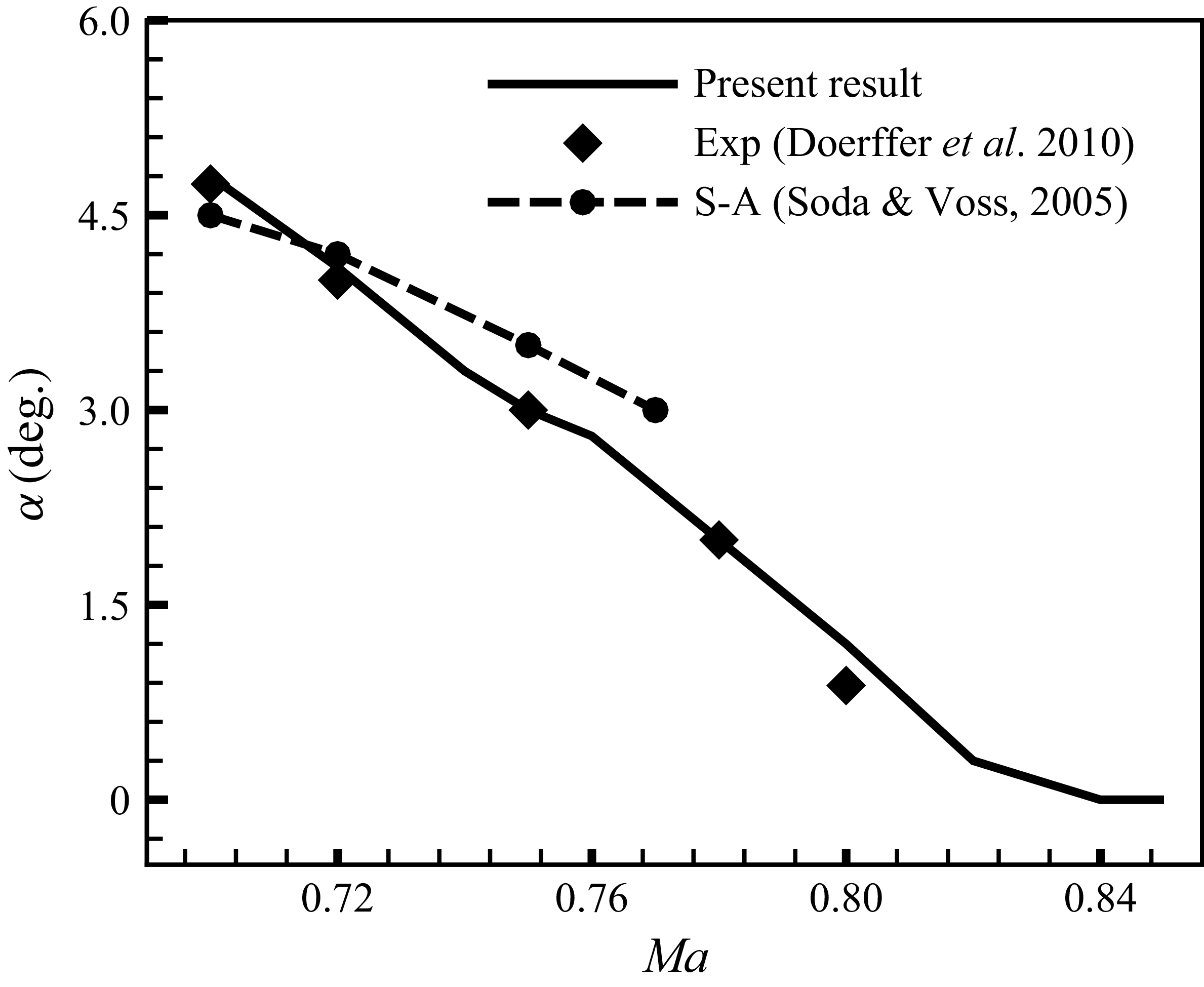
 Re=3×10⁶
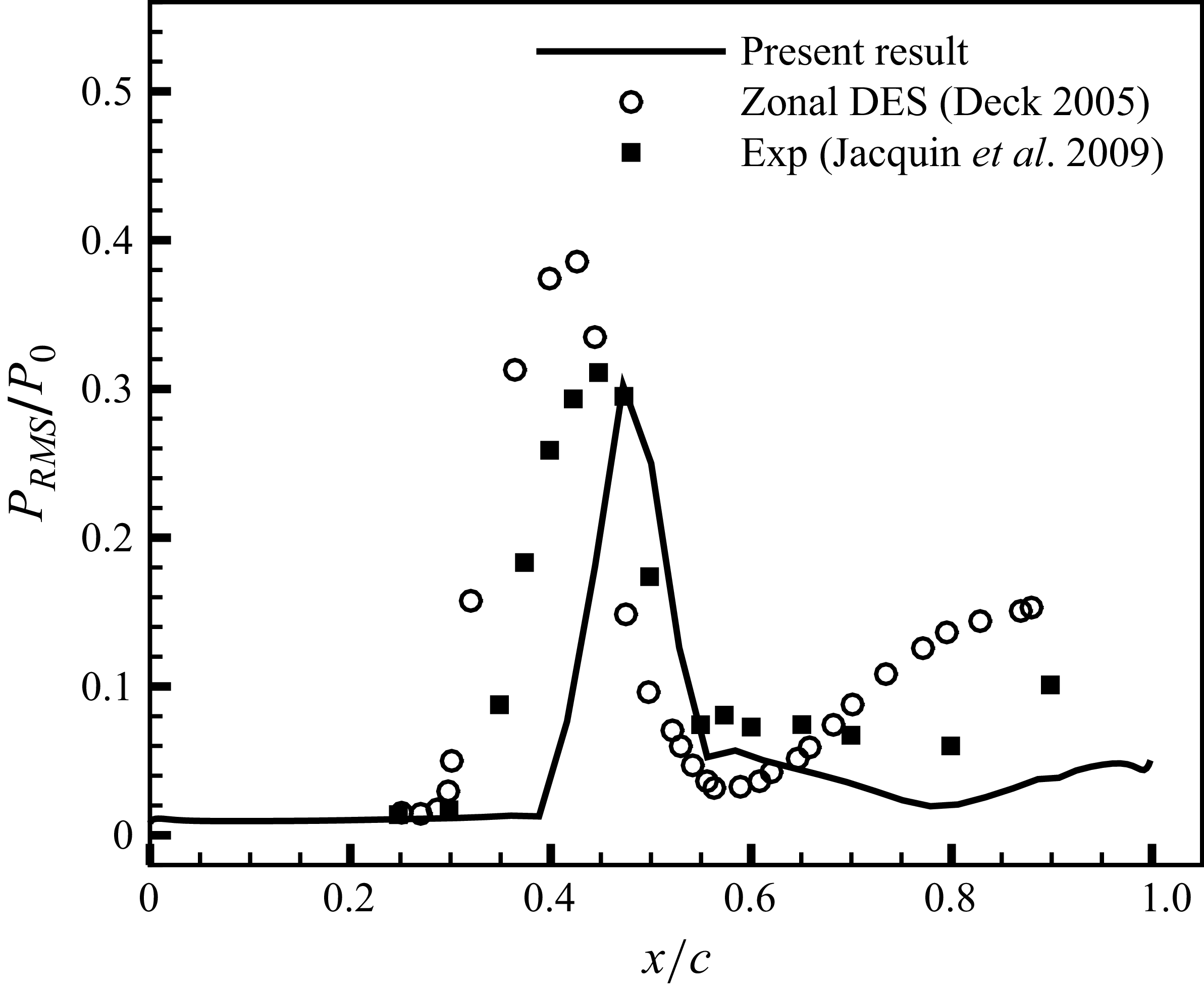
 Ma=0.73,α=3.5∘, Re=3×10⁶
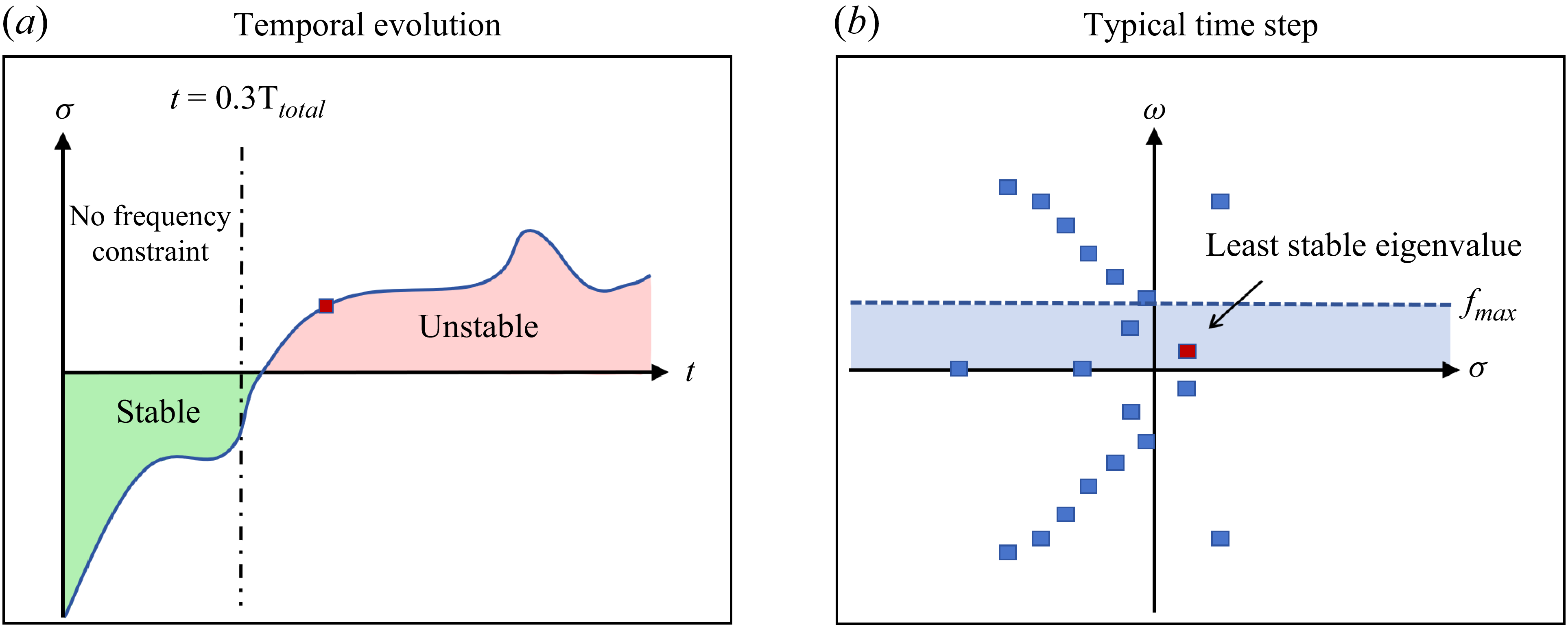


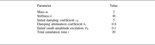
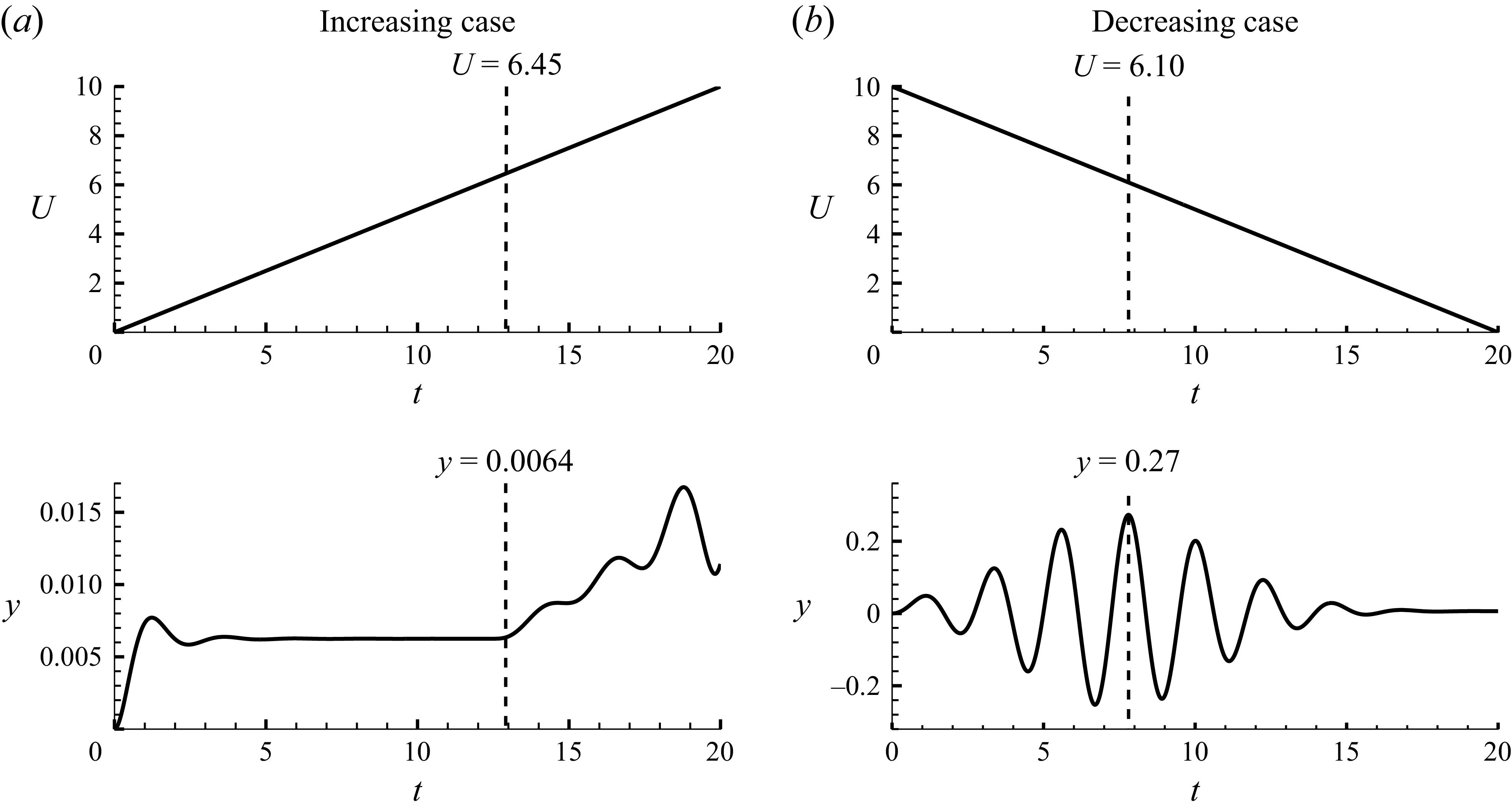
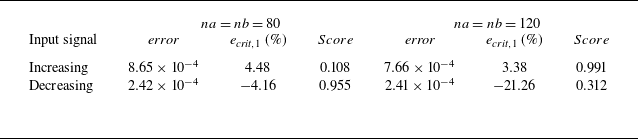


 Ma=0.7, α=5.5∘
 Re=3×10⁶



 Ma=0.7, α=5.5∘
 Re=3×10⁶
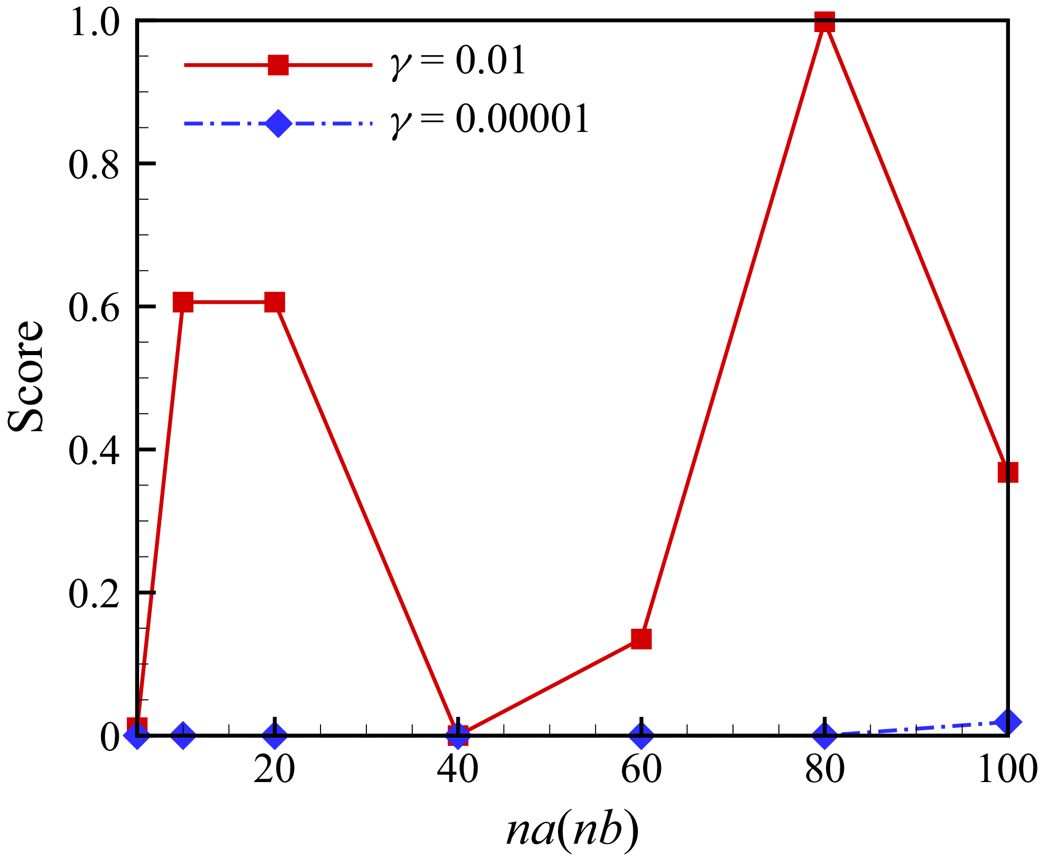

 Ma=0.7, α=5.5∘
 Re=3×10⁶

 Ma=0.7, α=5.5∘
 Re=3×10⁶
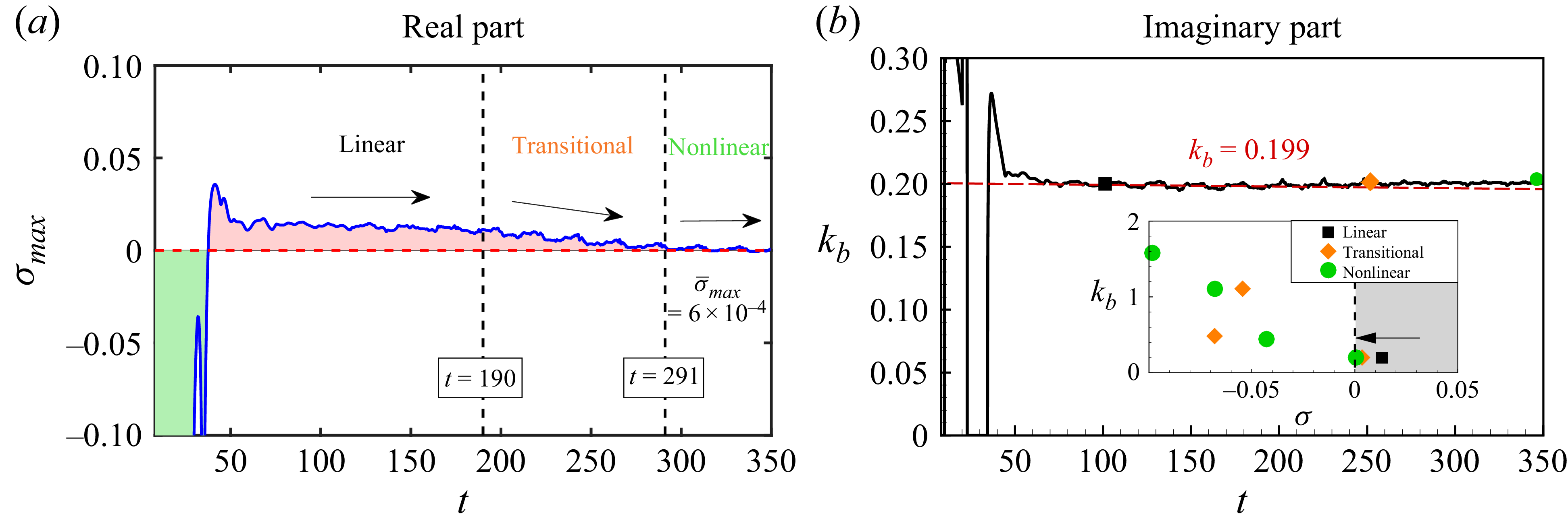
 Ma=0.7, α=5.5∘
 Re=3×10⁶


 Ma=0.70
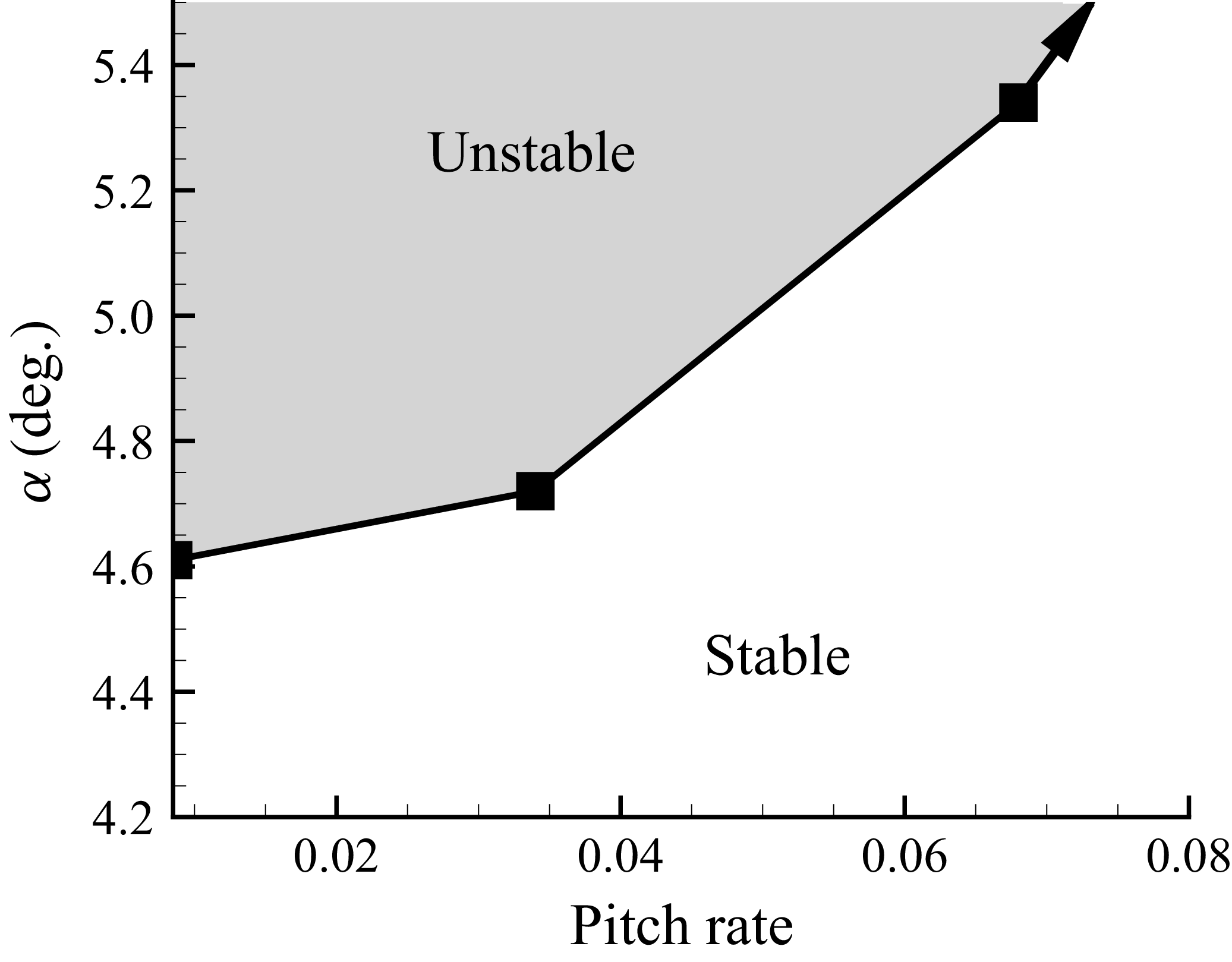
 Ma=0.70

 α=4.5∘
 Ma=0.70
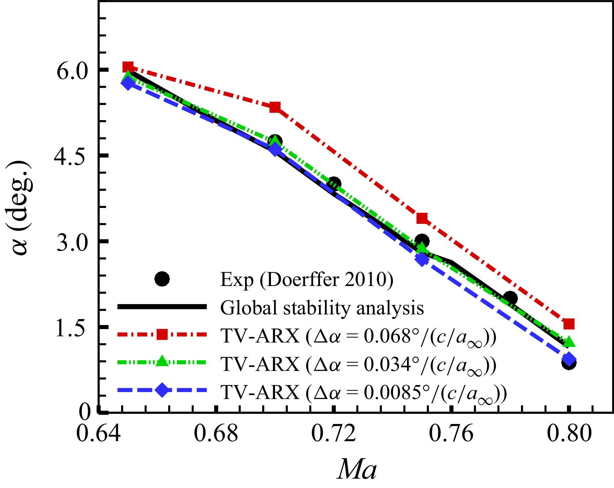
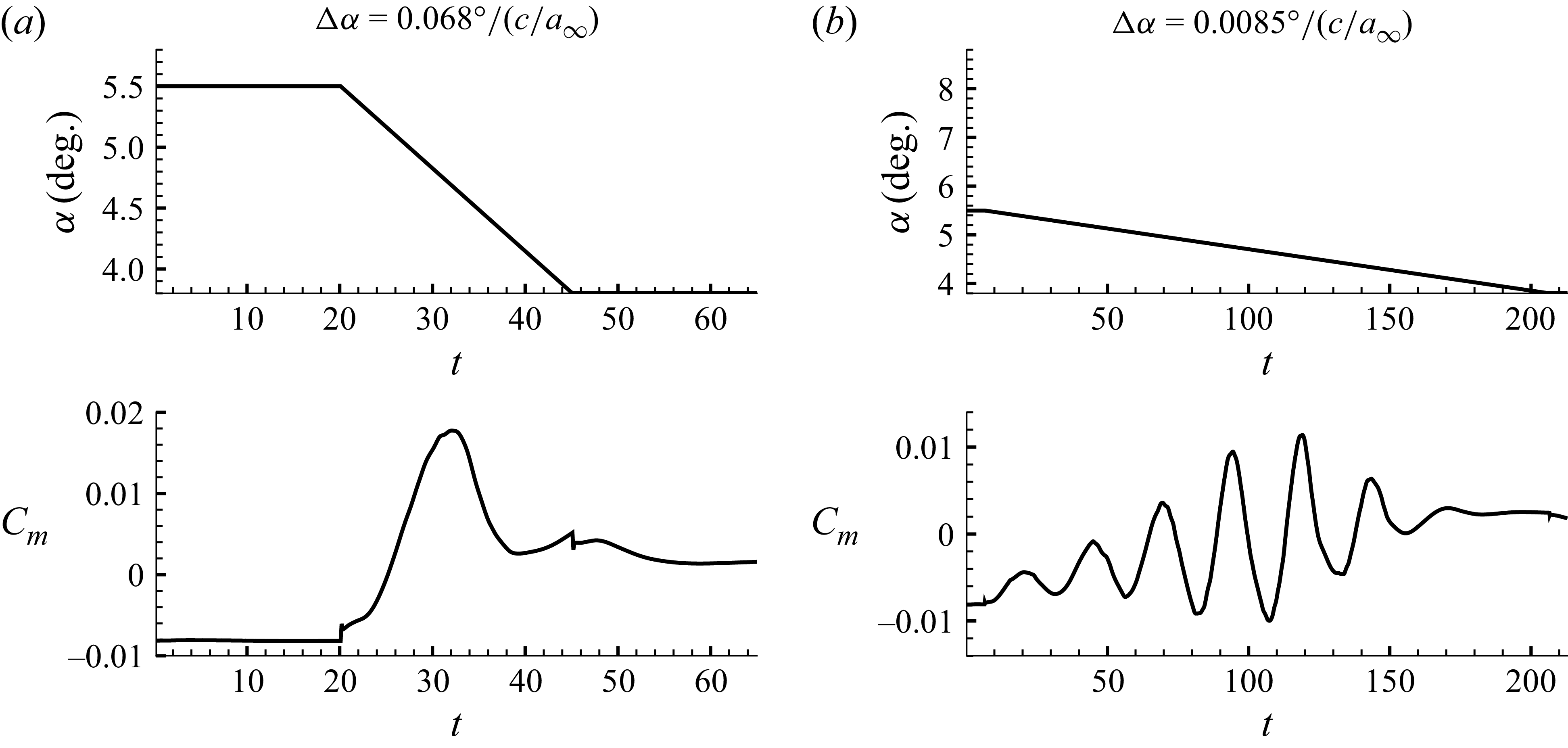
 M=0.70

 Ma=0.70
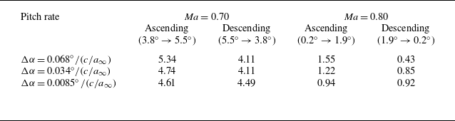

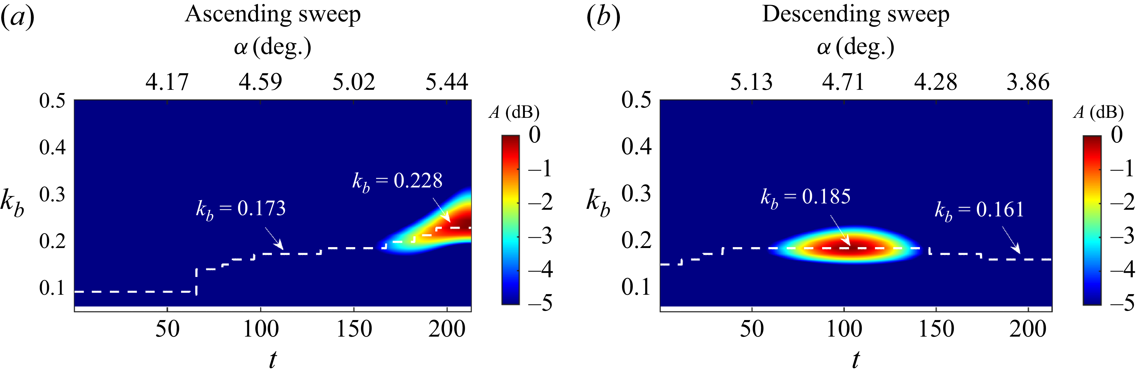
 Ma=0.70, Δα=0.0085∘/(c/a∞)

 Ma=0.70

 Ma=0.70, Δα=0.0085∘/(c/a∞)
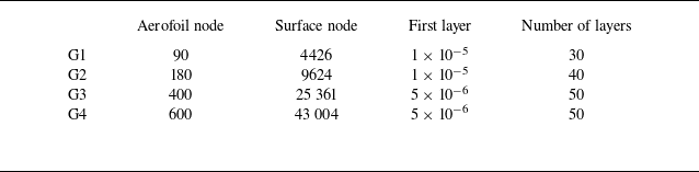
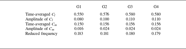
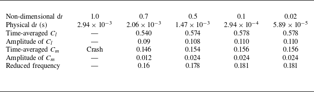
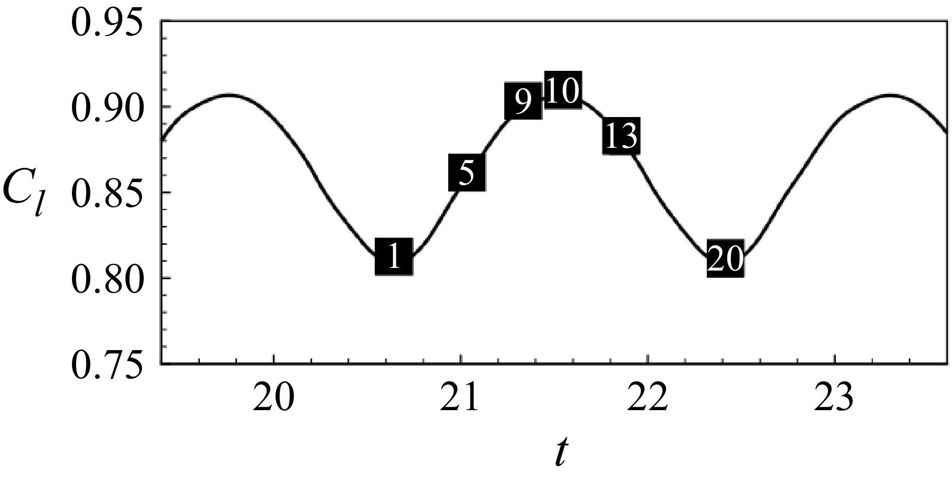

 x/c=0.6
 M=0.73
 α=3.7∘
 Re=3×10⁶

 γ

 Δα=0.034∘/(c/a∞)

 na=nb=80
 γ=0.01
 SNR=40
 SNR=20
 SNR=10


