Implications
For crossbred populations raised in extensive grazing conditions, effects of genotype by environment interaction as well as breed, heterozygosity, sex and contemporary group and sensitivity to the environment should be considered when designing breeding programs. Here, a model was developed for genetic evaluation of post-weaning weight gain by Nelore×Angus crossbred cattle. For estimation of genetic parameters and breeding values, heterogeneous additive genetic and residual variances were taken into account. Estimated heritability of post-weaning weight gain was considerably greater in favorable environments. Thus, greater selection response can be expected in these environments.
Introduction
Optimal design of a multi-breed population for use in diverse environments is likely to be characterized by differences in breed proportions varying with environmental conditions (Long, Reference Long1980; Arthur et al., Reference Arthur, Hearnshaw and Stephenson1999). Optimal proportions of Bos indicus (for adaptation) and Bos taurus (for production) breeds may vary with differences in both management and climate. Moreover, the deviation in performance of individual animals from their group means may be affected by genotype by environment (G×E) interaction. This interaction may cause re-ranking of animals based on their evaluations for different environments (Falconer and Mackay, Reference Falconer and Mackay1996). Evidence of G×E interaction was observed for post-weaning gain of Hereford (B. taurus) cattle between North and South America, where the animals were raised with harvested feeds and at grazing, respectively (Lee and Bertrand, Reference Lee and Bertrand2002). Occurrence of G×E interaction was observed in Nelore (B. indicus) between regions in the southeast (Ferreira et al., Reference Ferreira, Penna, Bergmann and Torres2001) and mid-west of Brazil (Toral et al., Reference Toral, Silva, Martins, Gondo and Simonelli2004), and for composite beef cattle in practically all Brazilian biomes (Amazon, Cerrado, Pantanal, Atlantic Rain Forest and Pampa) (Santana et al., Reference Santana, Eler, Cardoso, Albuquerque and Ferraz2013). Traditionally, G×E interaction has been described by treating phenotypic expressions in different environments as distinct traits and estimating genetic correlations among them (Costa et al., Reference Costa, Blake, Pollak, Oltenacu, Quaas and Searle2000; de Mattos et al., Reference de Mattos, Bertrand and Misztal2000). If the genetic correlations are not large (e.g. <0.8; Robertson, Reference Robertson1959) G×E interaction is established. Recent evidence suggests a need to further consider G×E in genetic evaluation for beef cattle raised in diverse environmental conditions (Williams et al., Reference Williams, Łukaszewicz, Bertrand and Misztal2012).
Use of reaction norms obtained by random regression provides an alternative way to verify the presence of G×E interaction (Calus et al., Reference Calus, Groen and de Jong2002; Kolmodin et al., Reference Kolmodin, Strandberg, Madsen, Jensen and Jorjani2002). Through covariance functions it is possible to determine prediction of breeding values in response to continuous gradations in the production environment (Kirkpatrick et al., Reference Kirkpatrick, Lofsvold and Bulmer1990). This approach also allows modeling of heterogeneous genetic and environmental variances and has been used successfully to identify G×E interaction effects on performance of dairy (Kolmodin et al., Reference Kolmodin, Strandberg, Madsen, Jensen and Jorjani2002; Shariati et al., Reference Shariati, Su, Madsen and Sorensen2007; Strandberg et al., Reference Strandberg, Brotherstone, Wall and Coffey2009) and beef (Corrêa et al., Reference Corrêa, Dionello and Cardoso2009; Cardoso et al., Reference Cardoso, Braccini Neto, Cardoso, Cobuci, IdO and Barcellos2011; Mattar et al., Reference Mattar, Silva, Alencar and Cardoso2011; Cardoso and Tempelman, Reference Cardoso and Tempelman2012; Santana et al., Reference Santana, Eler, Cardoso, Albuquerque and Ferraz2013) cattle. Hierarchical Bayes models have the flexibility necessary to fit these models (Sorensen and Gianola, Reference Sorensen and Gianola2002). Thus, objectives of this study were to: (1) evaluate effects of G×E interaction on post-weaning weight gain of the Nelore (NE)×Angus (AN) crossbred cattle; (2) to propose a robust reaction norm multiple-breed animal model in the presence of heteroscedastic variances and (3) assess consequences of employing this model for estimation of genetic parameters.
Material and methods
Data
The Embrapa Brangus-lineage Ibagé foundation herd, in which crossbreeding of Nelore (NE) and Angus (AN) was undertaken to produce a stabilized composite of 3/8 NE and 5/8 AN, provided data for this study. Data contained animals with breed proportions ranging from 100% AN to 75% NE. All animals were raised at Embrapa South Livestock Center, located in a subtropical climatic region of Southern Brazil. The nutritional environment was provided by year-round extensive grazing.
Body weights were recorded from 1956, coincident with the first generation of 3/8 NE×5/8 AN animals, until 1979. There were 6366 animals with recorded weaning weights (WW). Within year and season, animals were kept together after weaning and weighed monthly until they were two years old. Contemporary groups (CG) were formed from year, season of birth, sex, and date of weighing, with stratification by age such that the range in age within contemporary group was ⩽90 days. Further editing resulted in elimination of CG with less than four animals. Finally, connectedness among CG was evaluated based on the total number of genetic links (minimum 10), using AMC software (Roso and Schenkel, Reference Roso and Schenkel2006), and nine disconnected CG containing 44 animals were eliminated.
To determine the post-weaning weight gain (PWG), the BW obtained when average age within management group was nearest to 550 days (BW550) was used in the following equation: PWG=[(BW550−WW)/PWP]×345, where PWP is the post-weaning period in days. Thus, all PWG records were adjusted to a period of 345 days. Records that deviated from their contemporary group mean by more than 3.5 standard deviations were eliminated. After editing, 4016 phenotypic records remained for the subsequent analyses and the pedigree file contained an additional 803 ancestors including 100% NE females used for the first crosses.
Models and methodology
We evaluated two alternative linear models. Following Cardoso and Tempelman (Reference Cardoso, Rosa and Tempelman2004), the simpler model was a multiple-breed animal model (MAM). Consistent with the specification of Oliveira et al. (Reference Oliveira, Cardoso and Osório2010 and Reference Oliveira, Cardoso and Osório2011) it was:
 $$\eqalignno{ y_{{ijkl}} {\,=\,}\mu {\plus}cg_{i} {\plus}sex_{j} {\plus}\beta _{{AOD}} \left( {aod_{k} } \right){\plus}\beta _{{AOD^{2} }} \left( {aod_{k}^{2} } \right)\cr{\plus}\beta _{A} \left( {f_{l} } \right){\plus}\beta _{D} \left( {\delta _{l} } \right){\plus}\beta _{{AA}} \left( {2\left[ {1{\minus}f_{l} } \right]f_{l} } \right){\plus}u_{l} {\plus}e_{{ijkl}} $$
where y
ijkl
is the PWG record on the l
th animal of the j
th sex in the i
th CG and; μ=the overall mean; cg
i
=the random effect of the i
th CG (i=1, 2, …, 268), with cg
i
~
 $$N\left( {0,\sigma _{{cg}}^{2} } \right)$$
; sex
j
=the effect of the j
th sex (j=1, 2 and 3, for male, steer and female, respectively); β*’s are regression coefficients associated with age of dam in years (AOD, 2⩽AOD⩽12), fixed additive effect (A) for the AN breed, NE×AN dominance effect (D) and NE×AN additive×additive epistatic effect (AA); f
l
=the expected proportion of AN alleles and δ
l
=the average expected heterozygosity for animal l. Then, following Kinghorn (Reference Kinghorn1980), 2[1–f
l
]f
l
=the additive×additive epistatic coefficient for animal l; u
l
=the additive genetic effect of animal l
th, assuming that
 $${\bf u}{\,=\,}\left\{ {u_{l} } \right\}_{{l{\,=\,}1}}^{{4819}} \,\sim\,N\left( {0,{\bf G}} \right)$$
, where G=is the multiple-breed genetic (co)variance matrix that is a function of the breed-specific genetic variances for Angus
 $$\sigma _{{g(AN)}}^{2} $$
and Nelore
 $$\sigma _{{g(NE)}}^{2} $$
, and genetic relationships among animals (Lo et al., Reference Lo, Fernando and Grossman1993). The segregation variance between the two breeds was assumed null based on results obtained by Oliveira et al. (Reference Oliveira, Cardoso and Osório2010). Finally,
 $$e_{{ijkl}} \,\sim\,N(0,\sigma _{{e_{{ijl}} }}^{2} )\,=$$
is the residual error, with different assumptions about its variance (
 $$\sigma _{{e_{{ijl}} }}^{2} $$
) and distribution, which characterize the distinct models described below.
Second, a linear mixed reaction norm model was proposed to consider G×E interaction as follows:
 $$\eqalignno{ y_{{ijkl}} {\,=\,}\mu {\plus}cg_{i} {\plus}sex_{j} {\plus}\beta _{{AOD}} \left( {aod_{k} } \right){\plus}\beta _{{AOD^{2} }} \left( {aod_{k}^{2} } \right)\cr{\plus}\beta _{A} \left( {f_{l} } \right){\plus}\beta _{D} \left( {\delta _{l} } \right){\plus}\beta _{{AA}} \left( {2\left[ {1{\minus}f_{l} } \right]f_{l} } \right){\plus}a_{l} {\plus}\beta _{{AX}} \left( {f_{l} } \right)\hat{X}_{{cg_{i} }} \cr{\plus}\beta _{{DX}} \left( {\delta _{l} } \right)\hat{X}_{{cg_{i} }} {\plus}\beta _{{AAX}} \left( {2\left[ {1{\minus}f_{l} } \right]f_{l} } \right)\hat{X}_{{cg_{i} }} \cr{\plus}b_{l} \hat{X}_{{cg_{i} }} {\plus}e_{{ijkl}} $$
wherein the animal genetic value (u
l
) from model 1 was decomposed into intercept (or level) (a
l
) and slope (b
l
) that was applicable to an environmental gradient. This environmental gradient was based on the CG solutions (
 $$\hat{X}_{{cg_{i} }} $$
) from model 1. This specification was based on CGs, as used in genetic evaluation, representing the most elemental characterization of production environments. Thus, CG effects are natural covariate candidates for beef cattle reaction norms (Cardoso et al., Reference Cardoso, Braccini Neto, Cardoso, Cobuci, IdO and Barcellos2011; Mattar et al., Reference Mattar, Silva, Alencar and Cardoso2011; Cardoso and Tempelman, Reference Cardoso and Tempelman2012). Additional regression coefficients β
AX
, β
DX
and β
AAX
, were included in model 2 to evaluate interactions of the genetic coefficient effects (A, D and AA) with the environmental gradient. The terms in models 1 and 2 were otherwise similar.
The vectors of random effects corresponding to all animals,
 $${\bf a}{\,=\,}\left\{ {a_{l} } \right\}_{{l{\,=\,}1}}^{{4819}} $$
and
 $${\bf b}{\,=\,}\left\{ {b_{l} } \right\}_{{l{\,=\,}1}}^{{4819}} $$
were assumed be normally distributed about mean zero with (co)variance structure:
 $${\rm Var}\left( {\left[ {\matrix{ {\bf a} \cr {\bf b} \cr } } \right]} \right){\,=\,}\left[ {\matrix{ {{\bf G}_{a}^{{}} } & {{\bf G}_{{ab}}^{{}} } \cr {{\bf G}_{{ab}}^{{}} } & {{\bf G}_{b}^{{}} } \cr } } \right]$$
where: G a , G b , G ab are multiple-breed additive genetic covariance matrices for between intercepts, between slopes, and between intercepts and slopes of animals reaction norms. These matrices were formed by an extension of the proposed rules for multiple-breed populations (Lo et al., Reference Lo, Fernando and Grossman1993; Cantet and Fernando, Reference Cantet and Fernando1995) and are a function of the additive relationship between animals and breed-specific genetic variances:
 $${\bf G}_{{g{\rm (}c{\rm )}}} {\,=\,}\left[ {\matrix{ {\sigma _{{a{\rm (}c{\rm )}}}^{2} } & {\sigma _{{ab{\rm (}c{\rm )}}}^{{}} } \cr {\sigma _{{ab{\rm (}c{\rm )}}}^{{}} } & {\sigma _{{b{\rm (}c{\rm )}}}^{2} } \cr } } \right]$$
where for breed c (AN or NE):
 $$\sigma _{{a{\rm (}c{\rm )}}}^{2} $$
and
 $$\sigma _{{b(c)}}^{2} $$
=additive genetic variances of the reaction norm intercept and slope, respectively;
 $$\sigma _{{ab(c)}}^{{}} $$
=genetic covariance between reaction norm intercept and slope. As for the model specified by equation (1), the segregation variance between AN and NE was assumed null. Thus, five different models, varying in their complexity, were evaluated:
-
(1) Animal model (AM): the traditional model for genetic evaluation, based on equation (1), without G×E interaction, and assuming homogeneity of variances across breeds (
 $$\sigma _{{g(AN)}}^{2} {\,=\,}\sigma _{{g(NE)}}^{2} $$
) and homoscedasticity of residual variance (i.e.
$$\sigma _{{e_{{ijl}} }}^{2} {\,=\,}\sigma _{e}^{2} $$
for all combinations of i, j and l).
-
(2) Multiple-breed animal model with heteroscedastic Student’s t errors (MAMH): based on equation (1) with breed specific variances for AN and NE, but without considering G×E interaction. Here the residual variance specific to the record of animal l is determined by a multiplicative function of an overall residual variance
$(\sigma _{e}^{2} )$
and scalar multiplicative factors specific to CG
$(\tau _{{CG_{i} }} )$
, sex
$(\tau _{{S_{j} }} )$
, proportion of the AN breed
$(\gamma _{A} )$
and heterozygosity
$(\gamma _{D} )$
(i.e.,
$$\sigma _{{e_{{ijl}} }}^{2} {\,=\,}\sigma _{e}^{2} \tau _{{CG_{i} }} \tau _{{S_{j} }} \left( {\gamma _{A} } \right)^{{f_{l} }} \left( {\gamma _{D} } \right)^{{\delta _{l} }} w_{l}^{{{\minus}1}} $$
). A structural prior distribution was adopted for scalar CG effects on the residual variance, given by
$$\tau _{{CG_{i} }} \,\sim\,\gamma ^{{{\minus}1}} \left( {\eta ,\eta {\minus}1} \right)$$
, for all i; where
$\eta \,\gt\,1$
is a heteroscedasticity parameter. Thus, it follows that
$E(\tau _{{CG_{i} }} ){\,=\,}1$
with
$${\rm Var}(\tau _{{CG_{i} }} ){\,=\,}{1 \over {\eta {\minus}2}}$$
and, therefore, as
$\eta \to\infty$
the influence of CG on heteroscedasticity of the residual disappears (Cardoso et al., Reference Cardoso and Tempelman2005; Kizilkaya and Tempelman, Reference Kizilkaya and Tempelman2005). Additionally, w
l
=a weighting variable specific to the record of animal l with a distribution that is conditionally defined as
$$w_{l} \,\sim\,\gamma \left( {{\nu \over 2},{\nu \over 2}} \right)$$
for all l with w
l
>0, where ν>0 represents the degrees of freedom or robustness parameter. Therefore, the marginal data density is a Student’s t distribution with ν degrees of freedom (Lange and Sinsheimer, Reference Lange and Sinsheimer1993). -
(3) Reaction norm animal model (AMRN): based on the equation (2) and modeling the G×E interaction via reaction norms. Homogeneity of genetic variance between breeds was assumed (i.e.
${\bf G}_{{g(AN)}} {\,=\,}{\bf G}_{{g(NE)}} $
) and
$\sigma _{{e_{{ijl}} }}^{2} {\,=\,}\sigma _{e}^{2} (\gamma _{X} )^{{\hat{X}_{{cg_{i} }} }} $
was the residual variance specific to the record of animal l, determined by a multiplicative function of a global residual variance
$(\sigma _{e}^{2} )$
and a scale factor
$(\gamma _{X} )$
that relates the residual variance to the environmental level
$$\hat{X}_{{cg_{i} }} $$
. -
(4) Reaction norm animal model with heteroscedastic Student t errors (AMRNH): an animal model with G×E interaction and homogeneity of genetic variance between breeds, but assuming heteroscedastic residual variances, where
$\sigma _{{ejl}}^{2} {\,=\,}\sigma _{e}^{2} \tau _{{CG_{i} }} \tau _{{S_{j} }} (\gamma _{A} )^{{f_{l} }} (\gamma _{D} )^{{\delta _{l} }} (\gamma _{X} )^{{\hat{X}_{{cg_{i} }} }} w_{l}^{{{\minus}1}} $
=the residual variance specific to the record of animal l, with heteroscedasticity parameters as specified above in model 2 (MAMH). -
(5) Reaction norm multiple-breed animal model with heteroscedastic Student t errors (MAMRNH): the most complex adopted model based on equation (2) with G×E interaction and heteroscedastic genetic and residual variances, where
$\sigma _{{ejl}}^{2} {\,=\,}\sigma _{e}^{2} \tau _{{CG_{i} }} \tau _{{S_{j} }} (\gamma _{A} )^{{f_{l} }} (\gamma _{D} )^{{\delta _{l} }} (\gamma _{X} )^{{\hat{X}_{{cg_{i} }} }} w_{l}^{{{\minus}1}} $
as specified in models 2 (MAMH) and 4 (AMRNH) above.


Specification of priors
For all five models, bounded uniform priors were used for the fixed effects μ, sex
j
and β*’s. For the random effects of cg and u we assumed normal prior distributions as described above and conjugated relatively uninformative specifications for variance components as scaled inverted χ
2 prior densities:
 $$\sigma _{{cg}}^{2} \,\mid\,v_{{cg}} ,s_{{cg}}^{2} \,\sim\,s_{{cg}}^{2} \chi _{{cg}}^{{{\minus}2}} $$
and, for models without G×E interaction,
 $$\sigma _{{g(c)}}^{2} \,\mid\,v_{{g(c)}} ,s_{{g(c)}}^{2} \,\sim\,s_{{g(c)}}^{2} \chi _{{g(c)}}^{{{\minus}2}} $$
, c=AN or c=NE. The hyper-parameters represented by
 $$\nu _{{cg}} $$
, and
 $$\nu _{{g(c)}} $$
indicate the degree of belief in prior values of variances components
 $$\sigma _{{cg}}^{2} $$
and
 $$\sigma _{{g(c)}}^{2} $$
, given respectively by the hyper-parameters
 $$s_{{cg}}^{2} $$
and
 $$s_{{g(c)}}^{2} $$
. For reaction norms models, genetic variances are represented by the 2×2 matrix
 $${\bf G}_{{g(c)}} $$
with the a priori assumed
 $${\bf G}_{{g(c)}} \,\sim\,W^{{{\minus}1}} ({\bf T}_{{g(c)}} ,v_{{g(c)}} )$$
, that is,
 $${\bf G}_{{g(c)}} $$
had an inverse Wishart distribution, where
 $$\nu _{{g(c)}} $$
represents the degree of belief in prior values of variance components given by the hyper-parameters in
 $${\bf T}_{{g(c)}} $$
. Numeric values specified for the hyper-parameters were:
 $v_{{g(AN)}} {\,=\,}v_{{g(NE)}} {\,=\,}8$
;
 $v_{{cg}} {\,=\,}1$
;
 $s_{{g(AN)}}^{2} {\,=\,}s_{{g(NE)}}^{2} {\,=\,}150$
,
 $s_{{cg}}^{2} {\,=\,}1000$
and
 $${\bf T}_{{g(AN)}} {\,=\,}{\bf T}_{{g(NE)}} {\,=\,}\left[ {\matrix{ {150} & {1.5} \cr {1.5} & {0.2} \cr } } \right]$$
. For the residual variance, the prior density was
 $$\left. {\sigma _{e}^{2} } \right|\nu _{e} ,s_{e}^{2} \,\sim\,s_{e}^{2} \chi _{e}^{{{\minus}2}} $$
, with
 $v_{e} {\,=\,}1$
and
 $s_{e}^{2} {\,=\,}350$
. Finally, a γ distribution was specified a priori for the heteroscedasticity parameter η with hyper-parameters
 $\alpha _{n} {\,=\,}0.03$
and
 $\beta _{n} {\,=\,}0.01$
. This resulted in an expected value of
 $E(\eta ){\,=\,}3$
and prior variance of
 ${\mathop{\rm var}} \:(\eta ){\,=\,}300$
. Similarly, a γ prior density was adopted for the robustness parameter ν, with hyper-parameters
 $\alpha _{v} {\,=\,}0.04$
and
 $\beta _{v} {\,=\,}0.01$
, in Student’s t error models (MAMH, AMRNH, MAMRNH), such that the a priori expected value was
 $E(v){\,=\,}4$
.
Variance components and genetic parameters
Additive genetic variance for breed group g and environment X
 $(\sigma _{{A(g)}}^{2} \!\mid\!X)$
was calculated as a function of breed (co)variances weighted by breed composition, using the following equation:
 $$\eqalign{ \left. {\sigma _{{A(g)}}^{2} } \right|X{\,=\,}f_{{AN}}^{g} \left( {\sigma _{{a{\rm (}AN{\rm )}}}^{2} {\plus}X^{2} \sigma _{{b{\rm (}AN{\rm )}}}^{2} {\plus}2X\sigma _{{ab{\rm (}AN{\rm )}}}^{{}} } \right){\plus}f_{{NE}}^{g} \cr\left( {\sigma _{{a{\rm (}NE{\rm )}}}^{2} {\plus}X^{2} \sigma _{{b{\rm (}NE{\rm )}}}^{2} {\plus}2X\sigma _{{ab{\rm (}NE{\rm )}}}^{{}} } \right)$$
where
 $$f_{c}^{g} $$
= is the proportion of breed c observed in breed group g.
The marginal residual variance specific for breed group g given the environment X
 $$\left( {\left. {\sigma _{{e(g)}}^{2} } \right|X} \right)$$
depended upon the model assumption. For AM,
 $$\left. {\sigma _{{e(g)}}^{2} } \right|X{\,=\,}\sigma _{e}^{2} $$
and therefore there was one value for all g and X. For AMRN,
 $$\left. {\sigma _{{e(g)}}^{2} } \right|X{\,=\,}\sigma _{{e(g)}}^{2} \left( {\gamma _{X} } \right)^{X} $$
and thus the value was common to all g, but specific for each value of X. For MAMH,
 $$\sigma _{e(g)}^2 \,\mid\,X{\,=\,}{v \over {v{\minus}2}}\sigma _e^2 \tau _{S1}^{0.146} \tau _{S2}^{0.241} {\left( {\gamma _A } \right)}^{f_g } {\left( {\gamma _D } \right)}^{f_g } $$
and thus its value does not depend on X environment, but varies between breed groups by the breed proportion f
g
and heterozygosity δ
g
observed in group g. It should also be noted that
 $$E\left( {\tau _{{CG_{i} }} } \right){\,=\,}1$$
for all CG
i
. Sample proportions of male and castrated male animals were and 0.146 and 0.241, respectively. Finally, for AMRNH and MAMRNH,
 $$\left. {\sigma _{{e(g)}}^{2} } \right|X{\,=\,}{\nu \over {\nu {\minus}2}}\sigma _{e}^{2} \tau _{{S_{1} }}^{{0.146}} \tau _{{S_{2} }}^{{0.241}} \left( {\gamma _{A} } \right)^{{f_{g} }} \left( {\gamma _{D} } \right)^{{\delta _{g} }} \left( {\gamma _{X} } \right)^{X} $$
, which is a function of both environment and breed composition as described above.
Estimated heritability for breed group g in X environment is the ratio of genetic variance and phenotypic variances, as follows:
 $$\left. {h_{{A(g)}}^{2} } \right|X{\,=\,}{{\left. {\sigma _{{A(g)}}^{2} } \right|X} \over {\left. {\sigma _{{A(g)}}^{2} } \right|X{\plus}\left. {\sigma _{{e(g)}}^{2} } \right|X}}$$
Posterior inference
Inference was based on Markov Chain Monte Carlo (MCMC) methods using INTERGEN software (Cardoso, Reference Cardoso2010). For all five models, the MCMC chain ran for 110 000 cycles with the first 10 000 cycles discarded as burn-in and the remaining cycles thinned to every 10th sample. Summarization of the remaining samples yielded a posteriori estimates of means, modes, percentiles (0.025 and 0.975) and standard deviations of all parameters.
Model choice criterion
Deviance information criterion (DIC) (Spiegelhalter et al., Reference Spiegelhalter, Best, Carlin and van derLinde2002) and conditional predictive ordinate (CPO) (Gelfand, Reference Gelfand1996) were used to compare the fit of the evaluated models. The DIC provides a measure of overall fit and posterior mean of the deviance, with a penalty for model complexity. Following Spiegelhalter et al. (Reference Spiegelhalter, Best, Carlin and van derLinde2002), the deviance of Model M
r
is estimated by:
 $\bar{D}_{r} {\,=\,}{{\rm 1} \over G}\mathop{\sum}\limits_{l{\,=\,}1}^G {{\minus}{\rm 2logp}\left( {y\,\mid\,\theta ^{{\left( l \right)}} ,M_{r} } \right)} $
, where
 $\theta ^{{\left( l \right)}} $
includes the sampled value of all parameters of model M
r
in cycle l of G total cycles. The complexity of Model M
r
is determined by the effective number of parameter that it contains:
 $p_{D\left( r \right)} {\,=\,}\bar{D}_{r} {\minus}D_{r} \left( {\bar{\theta }} \right)$
, where
 $D_{r} \left( {\bar{\theta }} \right){\,=\,}{\rm {\minus}2logp} \left( {y\!\mid\!\bar{\theta },M_{r} } \right)$
with
 $\bar{\theta }$
being the posterior mean of θ. Thus, p
D(r) represents the difference between posterior mean deviance and deviance based on posterior mean of parameters in Model M
r
. Finally, DIC of model M
r
is:
 $DIC_{r} {\,=\,}\bar{D}_{r} {\plus}p_{D(r)}$
. Smaller values of DIC indicate better model fit and are preferable.
For observation y
ij
, the conditional predictive ordinate (CPO) is
 $p\left( {y_{{ij}} \,\mid\,y_{{\left( {{\minus}ij} \right)}} ,M_{r} } \right)$
. It is intended to be a cross-validation density which indicates values of y
ij
that are likely observed when model M
r
is fit to all other observations
 $y_{{\left( {{\minus}ij} \right)}} $
except y
ij
. Estimated CPOs for model M
r
were obtained by the harmonic mean of G cycles of MCMC, using the following approach (Gelfand, Reference Gelfand1996):
 $$p\left( {y_{{ij}} \,\mid\,y_{{\left( {{\minus}ij} \right)}} ,M_{r} } \right)\,\approx\,{1 \over {{\textstyle{1 \over G}}\mathop{\sum}\limits_{l{\,=\,}1}^G {p^{{{\minus}1}} \left( {y_{{ij}} \,\mid\,\theta ^{{(l)}} ,M_{r} } \right)} }}$$
An estimate of the deviance of model r based CPO was obtained by
 ${\minus}{\rm 2}\mathop{\sum}\limits_{k{\,=\,}1}^n {{\ri log\hat{p}}\left( {y_{k} \,\mid\,y_{{\left( k \right)}} ,M_{i} } \right)} $
, for which smaller values also indicate better fit.
Results and discussion
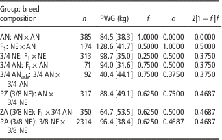
Number of records, mean and standard deviation of PWG, expected fraction of Angus alleles, expected fractions of heterozygosity and additive×additive epistasis are presented in Table 1 for the various combinations of AN and NE produced in the development of the Embrapa Brangus-lineage Ibagé foundation herd.
Number of records (n), mean [SD] post-weaning gain (PWG), expected fraction of Angus alleles (f), expected heterozygosity (δ) and additive×additive epistasis (2[1−f]f) for various breed combinations produced in forming the Embrapa Brangus-lineage Ibagé foundation herd

AN=Angus; NE=Nelore.
Model choice
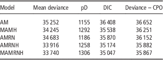
Results for model fit criteria, DIC and deviance based on CPO (Table 2), favored reaction norm models relative to models that did not contain the G×E interaction effect within same multiple-breed structure specification (AMRN v. AM and MAMRNH v. MAMH). Likewise, multiple-breed animal models were favored in relation to traditional animal models within the same specification of G×E interaction, that is, MAMRNH v. AMRNH and MAMH v. AM. The model that considered residual heteroscedasticity within the same specification for the G×E interaction also had the better fit to the PWG data (AMRNH v. AMRN). These results are in agreement with previous recommendations that heteroscedastic residual variances be considered for reaction norm applications (Calus et al., Reference Calus, Groen and de Jong2002, Cardoso and Tempelman, Reference Cardoso and Tempelman2012). Thus, heterogeneity of genetic and residual variances and G×E interaction should be jointly accounted for in PWG genetic evaluation of these Brangus cattle and specifically MAMRNH was the most suitable model (Table 2).
Variation among models in mean deviance, penalty for effective number of parameters (pD), deviance information criterion (DIC) and deviance from the conditional predictive ordinate (Deviance – CPO) for post-weaning weight gain

AM=animal model; MAMH=multiple-breed animal model with heteroscedastic Student’s t errors; AMRM=reaction norm animal model; AMRNH=reaction norm animal model with heteroscedastic Student’s t errors; MAMRNH=reaction norm multiple-breed animal model with heteroscedastic Student’s t errors.
Fixed genetic effects
Estimates of fixed genetic effects on PWG from the five models that were evaluated are presented in Table 3. The effect of breed proportion (β A ) was for PWG to increase with the AN contribution. However, β A was greater when the linear effect of breed proportion was estimated across the environmental gradient (β AX ); that is, AM and MAMH v. AMRN, AMRNH and MAMRNH. Effects of heterozygosity on PWG were favorable and similar in all models. The additive×additive epistatic effect had a consistently adverse effect on PWG. These results were consistent with previous findings that also identified favorable effects of dominance and negative effects of epistasis on weight gain in studies of NE×Hereford multiple-breed populations (Cardoso and Tempelman, Reference Cardoso, Rosa and Tempelman2004, Carvalheiro et al., Reference Carvalheiro, Pimentel, Cardoso, Queiroz and Fries2006).
Estimates of mean [SD] from posterior distributions of fixed genetic effects on post-weaning gain (kg) of Angus – Nelore crosses from the animal model (AM), multiple-breed animal model with heteroscedastic Student’s t errors (MAMH), reaction norm animal model (AMRN), reaction norm animal model with heteroscedastic Student’s t errors (AMRNH), and reaction norm multiple-breed animal model with heteroscedastic Student’s t errors (MAMRNH)

When the interaction between fixed genetic effects and environmental gradient (X-represented by CG solutions) was modeled (ANRN, ANRNH and MAMRNH), β
AX
and β
DX
were both positive (Table 3). Thus, AN proportion and heterozygosity effects were greater in favorable environments. Further, the estimated epistatic effect (
 $$\beta _{{AAX}} $$
) was more negative in restrictive environments (Table 3).
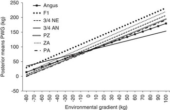
The relationship between breed groups and the environmental gradient is plotted in Figure 1 based on estimate from the MAMRNH model. It was observed that 3/4 NE animals responded to a lesser degree to the environmental improvement, since the linear reaction norm had the smallest slope among all the breed groups presented. The PWG of 3/4 NE was less than the performance of any other breed group. This result may be due to the breed additive effect and less expression of heterosis when compared with crosses with more intermediate breed proportions. However, the difference in breed additive effects is in contrast to the comparison of Angus and Nelore sire breeds used over Hereford dams in Texas, USA (Paschal et al., Reference Paschal, Sanders, Kerr, Lunt and Herring1995).
Posterior means for post-weaning weight gain (PWG) of different Angus (AN)×Nelore (NE) breed groups (F1: AN×NE or NE×AN; 3/4 NE: NE×F1 or F1×NE; 3/4 AN: AN×F1 or F1×AN; PZ (3/8 NE): AN×3/4 NE; ZA (3/8 NE): F1×3/4 AN; PA (3/8 NE): 3/8 NE×3/8 NE) across the contemporary group environmental gradient, obtained from the reaction norm multiple-breed animal model with heteroscedastic Student’s t errors (MAMRNH).

The PWG of AN was less than all other breed groups, except 3/4 NE. The purebred AN cattle lack the beneficial effects of heterosis and are commonly thought to be less well adapted to the subtropical climate conditions of Pampa Biome compared to animals with a greater percentage of indicine alleles. The F1 animals had the best performance across nearly the entire environmental gradient, except for extremely harsh environments. Finally, the different groups of 3/8 NE animals (PZ: AN×3/4 NE; ZA: F1 ×1/4 NE; and PA: 3/8 NE × 3/8 NE), had similar responses across the environmental gradient, with the superiority of PZ cattle being attributed to their greater level of expected heterozygosity (Table 1). This latter result is consistent with previous findings relative to the studied population (Oliveira et al., Reference Oliveira, Salomoni, Leal, Moraes and Del Duca1998).
Variance components and heritability
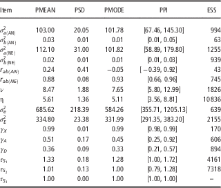
Genetic parameter estimates obtained from the best fitting model (MAMRNH) are presented in the Table 4. Presence of G×E interaction was indicated by existence of genetic variance for the reaction norm slopes (
 $$\sigma _{{b{\rm (}AN{\rm )}}}^{2} $$
and
 $$\,\sigma _{{b{\rm (}NE{\rm )}}}^{2} $$
in Table 4) and the better fit of the AMRN compared to AM (Table 2). The correlation between the intercept and slope of the reaction norm estimated from the posterior of the MAMRNH model differed between breeds (Table 4). For NE,
 $$r_{{ab{\rm (}NE{\rm )}}} $$
was positive and significant, indicating animals with higher average breeding values (level of the reaction norm) respond more to improved environmental conditions. This caused a scale G×E effect. The genetic variance for NE becomes greater as animals are exposed to superior environmental conditions. Thus, differences among animals in predicted genetic merit increased with improvement along the environmental gradient. However, animals would not necessarily change rank (Falconer and Mackay, Reference Falconer and Mackay1996). Similar substantial correlations between intercept and slope were also observed in previous studies of beef cattle where reaction norms were modeled. Examples from these studies include: Cardoso and Tempelman (Reference Cardoso and Tempelman2012) for Angus (0.95), Cardoso et al. (Reference Cardoso, Braccini Neto, Cardoso, Cobuci, IdO and Barcellos2011) for Hereford (0.97), Mattar et al. (Reference Mattar, Silva, Alencar and Cardoso2011) for Canchim (0.90) and Santana et al. (Reference Santana, Eler, Cardoso, Albuquerque and Ferraz2013) for tropical composite (0.94). In contrast, the 95% posterior probability support interval for
 $$r_{{ab{\rm (}AN{\rm )}}} $$
included zero, implying a non-significant correlation in our AN sample (Table 4). According to Su et al. (Reference Su, Madsen, Lund, Sorensen, Korsgaard and Jensen2006), a low posterior mean of correlation between intercept and slope as observed here for AN (
 $$r_{{ab{\rm (}AN{\rm )}}} $$
) indicates re-ranking of animals across environments. Thus, in the MAMRNH model, observed changes in the rank of animals for genetic merit across the environmental gradient likely results from the AN contribution. This correlation was the most distinct indication of difference between the two breeds. Overlapping 95% posterior probability support intervals for the reaction norm intercept and slope effects (Table 4) indicate their similarity.
Posterior mean (MEAN), posterior standard deviation (SD), posterior mode (MODE), 95% posterior support intervals (PPI), and effective sample size (ESS) for dispersion parameters obtained from the reaction norm multiple-breed animal model with heteroscedastic Student’s t errors for post-weaning gain in Angus (AN)×Nelore (NE) crosses

 $$\sigma _{{a{\rm (}c{\rm )}}}^{2} $$
=additive genetic variance of reaction norm intercept for c breed;
 $$\sigma _{{b{\rm (}c{\rm )}}}^{2} $$
=additive genetic variance of reaction norm slope for c breed;
 $$r_{{ab(c)}} $$
=additive genetic correlation between reaction norm intercept and slope for breed c; c=AN for Angus and c=NE for Nelore; ν=degrees of freedom or robustness; η=heteroskedasticity on contemporary groups;
 $$\sigma _{e}^{2} $$
=residual variance;
 $$\sigma _{E}^{2} $$
=marginal residual variance; γ
X
, γ
A
,γ
D
,
 $$\tau _{{S_{1} }} $$
,
 $$\tau _{{S_{2} }} $$
and
 $$\tau _{{S_{3} }} $$
=scaling factors for environmental gradient, proportion Angus, heterozygosity, male, steers, female (forced=1.0), respectively.
Based on results from the MAMRNH model (Table 4), residual variance decreased slightly (posterior means of γ
X
<1) as the environmental gradient increased. Despite being opposite in sign, these results were similar to those obtained by Cardoso et al. (Reference Cardoso, Braccini Neto, Cardoso, Cobuci, IdO and Barcellos2011), where residual variance increased slightly (scaling factor=1.007) as the environmental gradient indicated conditions that were more conducive to growth. Indications robustness and heteroscedasticity were similar to those obtained without considering G×E interaction for MAMH and by Oliveira et al. (Reference Oliveira, Cardoso and Osório2011). The a posteriori mean±SD of the robustness parameter (v) was near eight indicating the presence of outliers from the expected normal distribution of residues (Stranden and Gianola, Reference Stranden and Gianola1998). Residual heteroscedasticity among CG, as indicated by η, was high. Similar results were found by Kizilkaya and Tempelman (Reference Kizilkaya and Tempelman2005) for birth weight and calving ease scores in Italian Piedmontese breed and by Cardoso et al. (Reference Cardoso and Tempelman2005) for post-weaning weight gain in Nelore-Hereford crosses. Parameter estimates for γ
A
and γ
D
were less than 1 indicating that residual variability tended to decrease with increasing proportions of AN and heterozygosity. Finally, the residual variance was greater for bulls (
 $$\tau _{{S_{1} }} $$
) than for steers (
 $$\tau _{{S_{2} }} $$
) and heifers (
 $$\tau _{{S_{3} }} $$
). Similar residual heteroscedasticity associated with the sex effect has been previously observed for growth traits in beef cattle (Garrick et al., Reference Garrick, Pollak, Quaas and Vanvleck1989; Rodriguez-Almeida et al., Reference Rodriguez-Almeida, Vanvleck, Cundiff and Kachman1995).
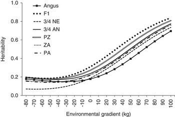
Heritability, indicating relative magnitude of the estimates of genetic and residual variances, may be more relevant to genetic evaluation. Greater environmental variation reduces heritability and a more uniform environment increases heritability (Falconer and Mackay, Reference Falconer and Mackay1996). The a posteriori mean estimates of PWG heritability from the MAMRNH model for different AN and NE breed groups were all directly proportional to the environmental gradient (Figure 2). Similar results have been found in other studies of post-weaning gain in beef cattle (Corrêa et al., Reference Corrêa, Dionello and Cardoso2009; Cardoso et al., Reference Cardoso, Braccini Neto, Cardoso, Cobuci, IdO and Barcellos2011; Mattar et al., Reference Mattar, Silva, Alencar and Cardoso2011; Cardoso and Tempelman, Reference Cardoso and Tempelman2012; Santana et al., Reference Santana, Eler, Cardoso, Albuquerque and Ferraz2013), and in dairy cattle for production and reproductive traits (Kolmodin et al., Reference Kolmodin, Strandberg, Madsen, Jensen and Jorjani2002; Shariati et al., Reference Shariati, Su, Madsen and Sorensen2007). These results indicate that heritability increases as environmental conditions improve. Toral et al. (Reference Toral, Silva, Martins, Gondo and Simonelli2004) hypothesized that genes expressed and the magnitude of their expression varies with the environment with more similar environments also sharing similar patterns of gene expression.
Posterior mean heritability of post-weaning gain (PWG) across the contemporary group environmental gradient for different Angus (AN)×Nelore (NE) breed groups (F1: AN×NE or NE×AN; 3/4 NE: NE×F1 or F1×NE; 3/4 AN: AN×F1 or F1×AN; PZ (3/8 NE): AN×3/4 NE; ZA (3/8 NE): F1×3/4 AN; PA (3/8 NE): 3/8 NE×3/8 NE), obtained from variance components estimated with the reaction norm multiple-breed animal model with heteroscedastic Student’s t errors (MAMRNH).

Conclusions
Multiple-breed models that consider genotype by environment interaction through reaction norms better explain variation among animals in performance than animal models traditionally used for genetic evaluations. Routine implementation of these more complex models could provide evaluations that enable greater response to selection for post-weaning weight gain of Brangus cattle raised under extensive conditions. Heritability estimates for post-weaning gain of Angus×Nelore crosses were considerably greater in favorable environments. Thus, greater selection response can be expected under improved rearing conditions.
Acknowledgments
The authors are grateful to Dr Michael D. MacNeil, Delta G, Miles City/MT, USA, for reviewing the manuscript and providing a constructive contribution to its final version; to Embrapa South Livestock Center for providing the data and to the National Council of Scientific and Technological Development (CNPq) for the fellowship granted to the first and third authors.