


1 Introduction
In view of its relevance to the tidal motion over topography in the oceans, internal wave radiation in stratified and rotating fluids has been investigated in detail for oscillating objects such as cylinders and spheres (see, for example, Flynn, Onu & Sutherland Reference Flynn, Onu and Sutherland2003; Onu, Flynn & Sutherland Reference Onu, Flynn and Sutherland2003; Voisin Reference Voisin2003; King, Zhang & Swinney Reference King, Zhang and Swinney2009; Voisin, Ermanyuk & Flór Reference Voisin, Ermanyuk and Flór2011). Internal waves were mainly found to diverge, away from the source region, and thus to decrease in energy. The oscillation of horizontally curved objects causes, due to the convergence of wave beams, a well-distinguishable focusing effect (Bühler & Muller Reference Bühler and Muller2007; Duran-Matute et al. Reference Duran-Matute, Flór, Godeferd and Jause-Labert2013; Ermanyuk, Shmakova & Flór Reference Ermanyuk, Shmakova and Flór2017). By conservation of momentum, the wave energy density increases with distance from the location of generation, since the wave beam cross-section decreases, thus causing an increase in amplitude. In situ observations in ocean canyons and straits (Buijsman, Legg & Klymak Reference Buijsman, Legg and Klymak2012; Vlasenko et al. Reference Vlasenko, Stashchuk, Inall, Porter and Aleynik2016) and curved mountains or craters (Peliz, Le Cann & Mohn Reference Peliz, Le Cann and Mohn2009; Dale & Inall Reference Dale and Inall2015) do show a high increase in internal wave amplitude. The ocean inside a deep submerged crater with a torus shape close to Portugal is found to be entirely mixed (Peliz et al. Reference Peliz, Le Cann and Mohn2009). These observations suggest that overturning due to wave focusing may be a potential candidate for local mixing processes in the oceans.
Theoretical considerations for a ring-shaped torus with Gaussian generatrix (Bühler & Muller Reference Bühler and Muller2007) suggest an amplitude amplification in the focal zone proportional to the square root of the torus aspect ratio, as is confirmed by experiments and energy arguments for a horizontally oscillating torus with a circular generatrix by Ermanyuk et al. (Reference Ermanyuk, Shmakova and Flór2017). In the present study, for low and moderate oscillation amplitudes, the focusing amplifies the internal wave amplitude almost two times in the focal zone, implying for a same wavelength a comparable increase in shear and isopycnal slopes. For a torus of aspect ratio
 $\unicode[STIX]{x1D716}=5$
and oscillation amplitude
 $A$
, the waves in the focal region were shown to be linear for
 $Ke<0.4$
, with
 $Ke=A/a$
the Keulegan–Carpenter number, and were compared successfully with the linear theory adapted from Hurley & Keady (Reference Hurley and Keady1997). When increasing the oscillation amplitude, nonlinear effects started at
 $Ke\approx 0.6$
and breaking occurred for
 $Ke>0.8$
, mainly in the focal region and far away from the oscillating object. Experimental and numerical investigation of inertial wave focusing in rotating fluids showed for very high amplitudes of oscillation the existence of wave-induced turbulence in the focal zone (Duran-Matute et al.
Reference Duran-Matute, Flór, Godeferd and Jause-Labert2013), which was used to study the effects of rotation on turbulence in isolation.
Here, we concentrate on the nonlinear aspects of wave focusing. The streaming instability that causes a mean flow and the triadic resonant instabilities, giving rise to the presence of lower harmonics, have recently been reviewed by Dauxois et al. (Reference Dauxois, Joubaud, Odier and Venaille2018). For a uniform two-dimensional wave beam, Bourget et al. (Reference Bourget, Dauxois, Joubaud and Odier2013) showed the presence of the triadic resonant instability, where in contrast to the parametric subharmonic instability, the resonant frequencies of the triad are not equal to half the dominant wave frequency. Dauxois et al. (Reference Dauxois, Joubaud, Odier and Venaille2018) stress the relevance of three dimensional and finite-width beam effects. Recent theoretical investigations by Kataoka & Akylas (Reference Kataoka and Akylas2016) and Fan, Kataoka & Akylas (Reference Fan, Kataoka and Akylas2018) discuss the instability of two wave beams which are unstable in three dimensions when they are separated, and/or have different angles of propagation. In the present study on focusing wave beams, the wave frequencies are equal, but due to the geometry of the focusing, wave beams are not parallel. The Reynolds stress increases towards the focal point and enhances a mean flow in the focal region. For high amplitudes, a triadic resonant instability generating two secondary waves of different frequencies and wavelengths is observed near the focal region. We discuss the effects of focusing on the mean flow generation and the observed triadic resonance.
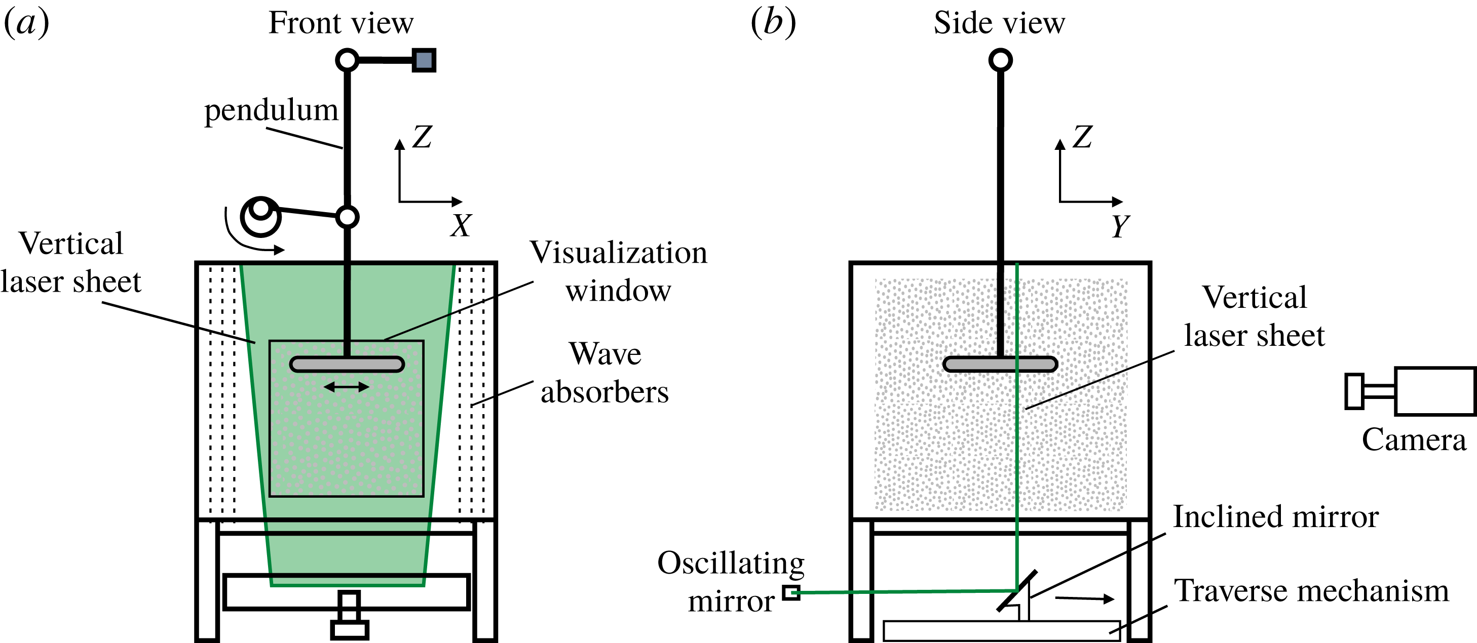
Sketch of the experimental set-up: (a) front view and (b) side view with the seeded particles as light grey dots and the laser plane shown in green.
The paper is organised as follows. Section 2 describes the experimental set-up and data processing methods, § 3 introduces the new non-dimensional focusing number and its relation to the Richardson number followed by the description of the focusing flow and mean flow towards the focal region in § 4. The resonant triadic wave interaction is reported in § 5, and the results are summarised and further discussed in § 6.
2 Experimental set-up and data processing
Experiments were carried out in a Plexiglas cubic tank of dimensions
 $97\times 97\times 97\;\text{cm}^{3}$
filled with a 85 cm deep linearly salt-stratified fluid. Internal waves were generated by horizontal oscillations of amplitude
 $A$
of a Plexiglas torus of minor radius
 $a=1,1.5$
or 2 cm and major radius
 $b=34$
, 13.5 or 10 cm, respectively. The aspect ratio, defined as
 $\unicode[STIX]{x1D716}=b/a$
, thus has values of 34, 9 or 5, respectively. To avoid wave reflections, the two side-walls of the tank perpendicular to the direction of oscillation were covered with a mesh of wave absorbers of 5 cm thickness (see figure 1).
The stratification was established with the standard double-bucket technique. The density was measured at different heights in the fluid with an Anton Paar density-meter. From these values the density profile was calculated, providing the buoyancy frequency
 $N=[(-g/\unicode[STIX]{x1D70C})\text{d}\unicode[STIX]{x1D70C}/\text{d}z]^{1/2}$
, with
 $g$
the gravitational acceleration and
 $\unicode[STIX]{x1D70C}(z)$
the density distribution over the vertical coordinate
 $z$
. The values of
 $N$
are presented in table 1.
To measure the flow in the vertical plane of symmetry
 $Y=0$
, the particle image velocimetry (PIV) method or the planar laser induced fluorescence (P-LIF) method was used. For the latter method, a grid of horizontally spanned cotton wires, painted with fluorescein dye, was dragged carefully through the fluid to generate a set of approximately 1 mm thick and equidistant horizontal dye planes before the experiment. These dye planes were illuminated by a vertical laser sheet. Diffusion of the dye gives a Gaussian distribution which, with subpixel resolution, allows for a very accurate localisation of the maximum, and therefore precise measurement of the wave motion (see Voisin et al.
Reference Voisin, Ermanyuk and Flór2011). For the PIV measurements, prior to the experiment, the fluid was seeded with
 $60~\unicode[STIX]{x03BC}\text{m}$
Orgasol® particles of density
 $\unicode[STIX]{x1D70C}=1.02~\text{kg}~\text{m}^{-3}$
, which were illuminated with a vertical laser sheet through the torus centre (see figure 1). Images were taken by a 12-bit Dalsa camera with a charge-coupled device (CCD) of
 $1024\times 1024~\text{pixels}$
. The particle displacement was obtained by cross-correlating two successive images using standard PIV techniques, and in particular, the UVMAT/CIVx software packages developed at LEGI providing the vertical
 $w(t)$
and longitudinal horizontal
 $u(t)$
velocities. (http://www.legi.cnrs.fr/web/spip.php?article763&lang=en.) In some experiments, the LIF technique that is described in detail in Voisin et al. (Reference Voisin, Ermanyuk and Flór2011), Ermanyuk, Flór & Voisin (Reference Ermanyuk, Flór and Voisin2011) was used (see table 1), and allowed calculation of the isopycnal slopes from the vertical displacement
 $\unicode[STIX]{x1D701}$
as
 $S(t)=\arctan (\unicode[STIX]{x0394}\unicode[STIX]{x1D701}/\unicode[STIX]{x0394}x)$
with a very high resolution, since it provided a continuous and sub-pixel signal in space. Below we are using the maximum isopycnal slope
 $S^{\ast }$
obtained for each LIF experiment in the focal region. To select the different wave modes and distinguish their propagation direction, the Hilbert transform method of Mercier, Garnier & Dauxois (Reference Mercier, Garnier and Dauxois2008) was used.
To locate the measurement results in space, in the following we define a Cartesian coordinate system with the origin at the centre of the torus at rest, the
 $z$
-axis pointing vertically upwards, and horizontal axis
 $x$
and
 $y$
respectively along and perpendicular to the direction of oscillation. These coordinates have been non-dimensionalised with the minor radius
 $a$
, so that
 $(X,Y,Z)=(x,y,z)/a$
, whereas the velocity components are normalised as
 $(U,V,W)=(u,v,w)/(A\unicode[STIX]{x1D714})$
, with
 $\unicode[STIX]{x1D714}$
the oscillation frequency. In table 1 the experimental parameters are presented.
Experimental parameters and measurement methods used, with
 $\unicode[STIX]{x1D716}=b/a$
the torus aspect ratio,
 $Ke=A/a$
the Keulegan–Carpenter number and
 $\unicode[STIX]{x1D714}/N$
the non-dimensional oscillation frequency.
 $Z$
is the measured region and
 $Z_{focal}$
corresponds to the geometrical point of intersection of the wave rays, both non-dimensionalized with
 $a$
. The focusing wave number
 $Fo$
is defined in § 3. Experiments B–E are also used in Ermanyuk et al. (Reference Ermanyuk, Shmakova and Flór2017).

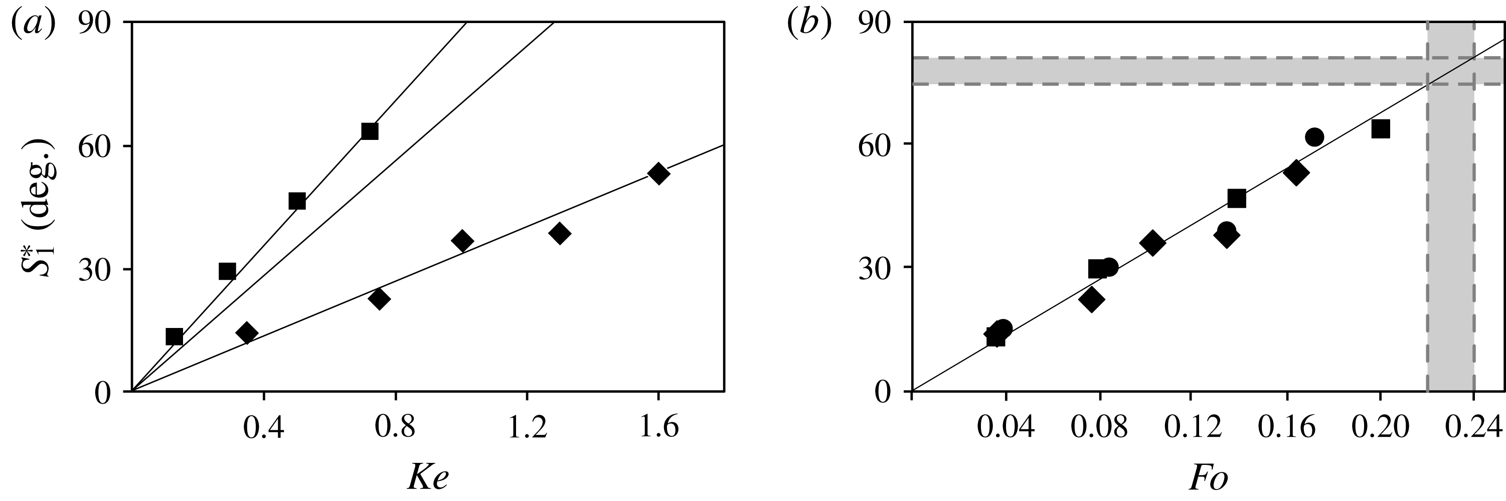
Maximum isopycnal slope attained during one period, against (a)
 $Ke$
and (b)
 $Fo$
numbers, with squares for the torus of
 $\unicode[STIX]{x1D716}=5$
at
 $Z=-6$
(Exp. D), circles for the torus of
 $\unicode[STIX]{x1D716}=9$
at
 $Z=-11.2$
(Exp. B) and diamonds for the torus of
 $\unicode[STIX]{x1D716}=34$
at
 $Z=-45$
(Exp. A). The error in the measurements is smaller than the size of the dots. The vertical grey area in (b) represents the critical focusing number
 $Fo=0.23\pm 0.01$
for overturning (see text) and the horizontal grey area the corresponding angle in isopycnal wave slope
 $78\pm 3^{\circ }$
. Experimental parameters are presented in table 1.
3 Focusing number
To characterise the generation of internal waves by an oscillating obstacle, the non-dimensional oscillation frequency
 $\unicode[STIX]{x1D714}/N$
and the Keulegan–Carpenter number,
 $Ke=A/a$
with
 $A$
the oscillation amplitude are generally used. The variation of the maximum waveslope as a function of
 $Ke$
is presented in figure 2(a) for tori with
 $\unicode[STIX]{x1D716}=5,9$
and 34, with each torus aspect ratio causing a different relation between isopycnal slope and excitation amplitude. This number is based on the maximum vertical displacement relative to the size of the object, and characterizes the wave amplitude close to the torus where the effects of curvature are hardly detectable. At large distances from the torus, however, the geometric effect of focusing causes a much larger wave amplitude. Thus each torus causes a different amplitude in the focal region (see figure 2
a). To uniformly predict the amplitude in the focal region, the length scale of the torus radius
 $b$
needs to be incorporated. The wave motion due to the fluid displacement of each segment of the torus is accumulated in the focal region. When integrated over the radius of the torus, this implies the additional length scale of the torus radius,
 $b$
. The length scale we propose is the geometric mean
 $\sqrt{ab}$
, also related to the surface of the torus
 $\unicode[STIX]{x03C0}^{2}ab$
, providing the adapted Keulegan–Carpenter number
 $$\begin{eqnarray}Ke^{\prime }=\frac{A}{\sqrt{ab}}=\frac{A/\unicode[STIX]{x1D716}^{1/2}}{a}.\end{eqnarray}$$
The value
 $\unicode[STIX]{x1D716}^{1/2}=(b/a)^{1/2}$
turns out to be the amplification of the amplitude in the focal region, and is also obtained from the energy estimations of the vertical displacement in the focal region of a torus (Ermanyuk et al.
Reference Ermanyuk, Shmakova and Flór2017) and Gaussian-shaped torus (Bühler & Muller Reference Bühler and Muller2007).
Since the wave amplitude varies significantly with the oscillation frequency (see Voisin et al. Reference Voisin, Ermanyuk and Flór2011), we also take into account this variation. Multiplying the wave amplitude with this factor (see Voisin et al. Reference Voisin, Ermanyuk and Flór2011), we obtain what we will further call the focusing number
 $$\begin{eqnarray}Fo=\frac{A}{a}\unicode[STIX]{x1D716}^{-1/2}\sin ^{1/2}\unicode[STIX]{x1D703}\cos \unicode[STIX]{x1D703}.\end{eqnarray}$$
For
 $\unicode[STIX]{x1D714}=0$
and
 $\unicode[STIX]{x1D714}=N$
, the focusing effect tends to zero, and it is maximal for
 $\unicode[STIX]{x1D703}=35^{\circ }$
.
The evolution of the maximum isopycnal slope against
 $Fo$
is presented in figure 2(b). All three tori with
 $\unicode[STIX]{x1D716}=5$
, 9 and 34 collapse on one line. This result suggests the focusing number as an appropriate non-dimensional parameter for converging waves. Below, we focus on the breaking in the focal region.
Richardson numbers
 $Ri_{PIV}$
from PIV data (grey symbols) for experiments Exp. C (circles), Exp. E (squares) and Exp. A (diamonds), and
 $Ri_{LIF}$
from LIF data (black symbols) for experiments Exp. B (circles), Exp. D (squares) and Exp. A (diamonds) with parameters given in table 1 in (a) a linear and (b) a logarithmic representation. The vertical grey lines denote the value of
 $Fo$
corresponding to the onset of overturning. The black dashed line in (b) represents the average trend of the data.

Flow variation in the vertical plane of symmetry, in the steady regime after 20 oscillation periods with (a,d,g,j)
 $Fo=0.053$
, (b,e,h,k)
 $Fo=0.16$
, and (c,f,i,l)
 $Fo=0.33$
; (a–c) instantaneous profiles of the horizontal velocity
 $U$
(colour) and contours of the horizontal transverse vorticity at phase
 $\unicode[STIX]{x03C0}/2$
(rightmost torus position); (d–f) shear stress
 $\overline{U^{\prime }W^{\prime }}$
; (g–i) vertical mean flow
 $W_{0}$
and (j–l) horizontal mean flow
 $U_{0}$
. The mean flow and shear stress are averaged over one period of oscillation. In images (g–l), the contours indicate the velocity amplitude. Exp. E from table 1.

3.1 Richardson and focusing numbers
In order to find the critical values of the focusing number for breaking, we plot the Richardson number as a function of the focusing number. In the linear approximation the vorticity equation for internal waves can be represented by a balance with the baroclinic torque given by
 $$\begin{eqnarray}\frac{\unicode[STIX]{x2202}\unicode[STIX]{x1D714}_{y}}{\unicode[STIX]{x2202}t}=\left(\frac{\unicode[STIX]{x1D735}p\times \unicode[STIX]{x1D735}\unicode[STIX]{x1D70C}}{\unicode[STIX]{x1D70C}^{2}}\right)_{y}=\frac{1}{\unicode[STIX]{x1D70C}^{2}}\left(\frac{\unicode[STIX]{x2202}p}{\unicode[STIX]{x2202}z}\frac{\unicode[STIX]{x2202}\unicode[STIX]{x1D70C}}{\unicode[STIX]{x2202}x}-\frac{\unicode[STIX]{x2202}p}{\unicode[STIX]{x2202}x}\frac{\unicode[STIX]{x2202}\unicode[STIX]{x1D70C}}{\unicode[STIX]{x2202}z}\right)\approx -\frac{g}{\unicode[STIX]{x1D70C}}\frac{\unicode[STIX]{x2202}\unicode[STIX]{x1D70C}}{\unicode[STIX]{x2202}x},\end{eqnarray}$$
where for the latter equality the Boussinesq approximation is used. Considering the ratio between stratification and the shear, here represented by the baroclinic torque, one obtains for the Richardson number
 $$\begin{eqnarray}Ri_{LIF}=N^{2}\left(\frac{\unicode[STIX]{x1D735}p\times \unicode[STIX]{x1D735}\unicode[STIX]{x1D70C}}{\unicode[STIX]{x1D70C}^{2}}\right)_{y}^{-1}\approx \frac{N^{2}}{\displaystyle \frac{-g}{\unicode[STIX]{x1D70C}}\frac{\unicode[STIX]{x2202}\unicode[STIX]{x1D70C}}{\unicode[STIX]{x2202}x}}=\left.\frac{\unicode[STIX]{x0394}x}{\unicode[STIX]{x0394}z}\right|_{\unicode[STIX]{x1D70C}}=\frac{1}{\tan S}.\end{eqnarray}$$
From the steepness
 $\unicode[STIX]{x0394}x/\unicode[STIX]{x0394}z$
of the P-LIF dye-lines the Richardson number could be measured accurately because of the sub-pixel resolution obtained with the Gaussian dye distribution mentioned above. In addition, the Richardson number in the focal region was calculated as
 $Ri_{PIV}=N^{2}/(\unicode[STIX]{x2202}u/\unicode[STIX]{x2202}z)^{2}\approx N^{2}/(\unicode[STIX]{x0394}u/\unicode[STIX]{x0394}z)^{2}$
, with
 $N$
the stratification measured prior to the experiment and the variation in velocity
 $\unicode[STIX]{x0394}u$
measured from the PIV data over a typical grid distance of
 $\unicode[STIX]{x0394}z=4$
pixels corresponding to
 ${\approx}0.15~\text{cm}$
. The values of this number are displayed in grey in figure 3(a) and in a log–log form in figure 3(b), and show that the values for both Richardson numbers,
 $Ri_{PIV}$
and
 $Ri_{LIF}$
, collapse on one curve.
Nonlinear effects, such as the generation of a mean flow and evanescent second harmonics were noticed around a value of
 $Fo\approx 0.1$
, corresponding to
 $Ri\approx 1.5$
. The asymptotic limit of
 $Ri\approx 0.25$
, corresponds to overturning in stratified shear flows (see Miles Reference Miles1961). The empirical relation between the Focusing number and the Richardson number can be estimated with the least-squares approximation as (see figure 3)
 $$\begin{eqnarray}Fo=(9\pm 0.5)Ri^{-2/3},\end{eqnarray}$$
and allows one to predict the breaking in focal regions for
 $Fo>0.23\pm 0.01$
as a function of the initial forcing parameters
 $a,b,A$
and the oscillation frequency given by
 $\unicode[STIX]{x1D703}$
. Applying this focusing number estimation on figure 2(b) one obtains the isopycnal slope
 $78\pm 3^{\circ }$
for breaking waves.
4 Observations
Figure 4(a–c) shows the change in the instantaneous horizontal velocity of the wave pattern in the vertical plane of symmetry
 $Y=0$
for increasing values of
 $Fo$
. One-half period later the direction of the velocity is reversed, implying a standing wave motion in the focal zone. The temporal motion in the focal region is therefore oscillatory, like a standing wave. This wave motion consists of the first harmonic, with all higher harmonics being evanescent since
 $\unicode[STIX]{x1D714}/N>0.5$
, the wave structure having the same dipolar shape as that observed for spherical objects in Shmakova, Ermanyuk & Flór (Reference Shmakova, Ermanyuk and Flór2017). The amplitude of the converging waves remains approximately constant. With increasing
 $Fo$
number from 0.053 to 0.16 (in respectively figures 4
a, 4
b), a clear increase in wave amplitude can be noticed. The vorticity contours coincide with the wave contours as long as wave breaking is absent, as shown in figure 4(a,b), while for
 $Fo=0.33$
in figure 4(c), the vorticity contours reveal the presence of breaking wave structures.
Figure 4(d–f) shows the non-dimensional shear stress,
 $\overline{U^{\prime }W^{\prime }}$
, averaged over one period. In the linear regime (
 $Fo<0.1$
, see figure 4
d), it is negligible for the outward moving (diverging) wave beams but is nonzero for the converging (focusing) wave beams, suggesting that the conical geometry of the focusing wave has a direct effect on the shear stress also. Since the wave amplitude in the focusing wave beam increases, intrinsically also
 $U^{\prime }$
and
 $W^{\prime }$
increase, giving rise to larger shear stress (see figure 4
e).
It is its gradient that is responsible for the mean flow towards the focal region (Fan et al.
Reference Fan, Kataoka and Akylas2018), leading to a strong vertical motion there, as shown in figure 4(h). Viscous dissipation towards the focal region, which is an essential ingredient for the streaming instability (see Fan et al.
Reference Fan, Kataoka and Akylas2018), is, however, overtaken by the effect of focusing. In the fully nonlinear regime, for
 $Fo>0.23$
, due to wave breaking the beam loses its coherence, and its direction is locally bent due to nonlinear interactions with the waves (figure 4
f).
The mean flow is shown in figure 4(g–i) for the
 $Y=0$
-symmetry plane. In the linear regime
 $Fo<0.1$
, it is small but non-negligible with very small amplitudes
 $O$
(0.06) for the mean vertical velocity. In the nonlinear regime
 $Fo>0.1$
, the motion in the focal region resembles a plume motion (see figure 4
g–i). Since the torus is oscillating horizontally there is, however, no axial symmetry, but the amplitude decreases away from the mid-plane
 $Y=0$
(see Ermanyuk et al.
Reference Ermanyuk, Shmakova and Flór2017).
When breaking occurs for
 $Fo>0.23$
(figure 4
c,f,i,l) the structure in the mean vertical and mean horizontal velocities remain clearly distinguishable, but the temporal horizontal motion (see figure 4
c) is affected by breaking as well as the presence of the wave triads that are discussed further below.
5 Triadic resonance and breaking in the focal zone
Patterns of the horizontal velocity
 $U$
(figure 4
a–c) show that for small
 $Fo$
values, the focal zone is represented by a standing wave. For large
 $Fo>0.23$
, new internal waves are generated, which are subharmonics, as their lower angle of propagation reveals. The time-frequency spectrum for the energy was obtained from vertical and horizontal components of the velocity
 $E_{uv}=(u^{2}+w^{2})/2$
defined by
 $$\begin{eqnarray}Q_{E_{uv}}(t,\unicode[STIX]{x1D714})=\left\langle \left|\int _{-\infty }^{+\infty }\,\text{d}\unicode[STIX]{x1D70F}~E_{uv}(\unicode[STIX]{x1D70F})\exp ^{-\text{i}\unicode[STIX]{x1D714}\unicode[STIX]{x1D70F}}h(t-\unicode[STIX]{x1D70F})\right|^{2}\right\rangle _{xz},\end{eqnarray}$$
where
 $h(t)$
is a Hamming window, and the average is taken over an interrogation area
 $xz$
around the focal region (Flandrin Reference Flandrin1998). The corresponding energy spectrum for
 $Fo=0.33$
is presented in figure 5, and shows clearly the generation of the first harmonic and two subharmonics, which satisfy
 $$\begin{eqnarray}\unicode[STIX]{x1D714}^{0}=\unicode[STIX]{x1D714}^{1}+\unicode[STIX]{x1D714}^{2},\end{eqnarray}$$
with
 $\unicode[STIX]{x1D714}^{0}$
the frequency of the first harmonic, and
 $\unicode[STIX]{x1D714}^{1}$
and
 $\unicode[STIX]{x1D714}^{2}$
the frequencies of first and second subharmonics, respectively. Using the Hilbert transform method of Mercier et al. (Reference Mercier, Garnier and Dauxois2008), the signal was filtered around a certain frequency in time for each harmonic (see figure 6
a–c), and then, to obtain the phase propagation, filtered for the direction shown in figure 6(d–f). In figure 6 we consider the positive direction of the first harmonic and subharmonic waves, and the negative direction of the second subharmonic of the triad. The standing wave motion, generated in the focal zone by the two opposite moving waves, is thus not visible. The first harmonic with frequency
 $\unicode[STIX]{x1D714}/N=0.8$
and algebraic amplitude of wave vector
 $\boldsymbol{k}>0$
in figure 6(a) shows an increasing amplitude towards the focal region, a local decrease in the zone of nonlinear interaction, and a decrease afterwards. Both subharmonic waves are generated in the focal zone, with the first subharmonic moving downwards (
 $k_{z}>0$
) and the second subharmonic moving upwards (
 $k_{z}<0$
) with frequencies of
 $\unicode[STIX]{x1D714}/N=0.6$
and
 $\unicode[STIX]{x1D714}/N=0.2$
, respectively. In contrast to the subharmonic wave with
 $\unicode[STIX]{x1D714}/N=0.6$
, the structure of the second subharmonic (
 $\unicode[STIX]{x1D714}/N=0.2$
) in figure 6(c) is confined to the breaking wave region shown in the instantaneous and the average horizontal velocities of figures 4(c) and 4(l), respectively, thus suggesting a strong interaction with the wave breaking. These first harmonic and subharmonic waves form together a triadic resonance, satisfying the condition
 $$\begin{eqnarray}\boldsymbol{k}^{\mathbf{1}}+\boldsymbol{k}^{\mathbf{2}}=\boldsymbol{k}^{\mathbf{0}},\end{eqnarray}$$
where
 $(k_{x}^{1}+k_{x}^{2})/k_{x}^{0}=0.96\pm 0.04$
and
 $(k_{z}^{1}+k_{z}^{2})/k_{z}^{0}=1.01\pm 0.01$
, with
 $k_{x}$
and
 $k_{z}$
selected from the space spectrum. This triadic resonance was found in all experiments for values of
 $Fo>0.23$
. Even though this flow differs from former studies in being fully three-dimensional and in that the waves focus, the triad interaction in wave-vector space in figure 5(b) shows a striking resemblance with figure 5 of Bourget et al. (Reference Bourget, Dauxois, Joubaud and Odier2013) for the triadic resonant instability in a flow that was in good approximation two-dimensional. Also the accuracy of the selected wave vectors is comparable to that in Brouzet et al. (Reference Brouzet, Sibgatullin, Scolan, Ermanyuk and Dauxois2016). Increasing the curvature, and therewith the three-dimensionality of the flow by taking a smaller torus (i.e. smaller
 $b$
) of larger cross-section (thickness
 $a$
), did not change the result, as shown for
 $\unicode[STIX]{x1D716}=5$
and
 $\unicode[STIX]{x1D716}=9$
in figure 5.
(a) Energy spectrum
 $\log _{10}(Q_{E_{uw}}(t,\unicode[STIX]{x1D714})/Q_{0})$
for the wave energy
 $E_{uw}$
with the non-dimensional frequency
 $\unicode[STIX]{x1D714}/N$
averaged over five periods of oscillations after reaching the steady regime for the thick (
 $\unicode[STIX]{x1D716}=5$
) torus with
 $Fo=0.33$
. Here,
 $Q$
is defined by (5.1) and
 $Q_{0}=\max [Q_{E_{uw}}(t,\unicode[STIX]{x1D714}^{0})]$
. The positions of the first harmonic (
 $\unicode[STIX]{x1D714}^{0}$
) and two subharmonics (
 $\unicode[STIX]{x1D714}^{1,2}$
) are shown with vertical dashed lines. (b) Resonance in wave-vector space (solid line) as calculated for a two-dimensional flow (see Bourget et al.
Reference Bourget, Dauxois, Joubaud and Odier2013). The scaled vectors are
 $k_{x}^{1}/k_{x}^{0}=1.53$
,
 $k_{z}^{1}/k_{z}^{0}=2.95$
(red);
 $k_{x}^{2}/k_{x}^{0}=-0.57$
,
 $k_{z}^{2}/k_{z}^{0}=-1.95$
(green); and black for the scaled vector
 $\boldsymbol{k}^{0}$
. Measurements of Exp. E (lines) and for Exp. C (dashed).

Hilbert decomposition in time and space of instantaneous horizontal velocity profile (a–c) and phase velocity (d–f) for
 $Fo=0.33$
. (a,d) First harmonic
 $U^{1}$
with frequency
 $\unicode[STIX]{x1D714}^{1}/N=0.8$
and
 $k_{z}>0$
; subharmonics with (b,e)
 $\unicode[STIX]{x1D714}_{1}/N=0.6$
,
 $k_{z}>0$
, and (c,f)
 $\unicode[STIX]{x1D714}_{2}/N=0.2$
,
 $k_{z}<0$
. (Exp. E from table 1).

6 Conclusions and discussion
To characterise focusing wave fields, the number
 $Fo$
has been introduced, indicating a linear regime for
 $Fo<0.1$
, a non-linear regime for
 $Fo>0.1$
, and wave breaking in the focal region for values larger than
 $Fo\approx 0.23$
. This wave breaking occurs at an isopycnal slope of
 $78\pm 3^{\circ }$
, in agreement with observations of Ermanyuk et al. (Reference Ermanyuk, Shmakova and Flór2017) and corresponding to a value of the Richardson number of
 $Ri=0.25$
for shear instability, and coincides with the presence of triadic resonance. In wave-vector space, this triad is very similar to the triad found by Bourget et al. (Reference Bourget, Dauxois, Joubaud and Odier2013). Indeed, the present flow with the maximum amplitude in the symmetry plane
 $Y=0$
(see Ermanyuk et al.
Reference Ermanyuk, Shmakova and Flór2017) is similar to the two-dimensional flow of Bourget et al. (Reference Bourget, Dauxois, Joubaud and Odier2013), which is limited by viscous boundaries. These results suggest that the three-dimensional effects due to the curvature of the wave generator, and consequent focusing, have little qualitative effect on the triadic resonant instability. However, the wave focusing plays an important role by creating a high energy density in the focal region, thereby providing a necessary condition for the onset of the instability.
The focusing number allows for an estimation of the onset of breaking in real flows. For a typical Keulegan–Carpenter number of
 $Ke=0.1$
in the ocean we can calculate the value of
 $\unicode[STIX]{x1D716}^{1/2}$
needed to reach the critical focusing number
 $Fo=0.23$
. For 12 hours
 $M_{2}$
tidal oscillation-frequency
 $\unicode[STIX]{x1D714}_{M2}$
, and typical ocean stratification
 $N\approx \unicode[STIX]{x1D714}/0.3$
, we obtain with (3.2) a value for
 $\unicode[STIX]{x1D716}^{1/2}$
of approximately 4.6, implying a major radius roughly 22 times larger than the minor radius. For large mountains, there may not be a continuity in curvature, and the focal point may be reached after reflection at the surface. But for an internal wave amplitude of 50 m and a mountain of 500 m width, this implies a large radius of 11 km indicating that focusing can cause wave breaking locally in specific places in the ocean, such as the craters mentioned in the introduction.
Acknowledgements
The authors acknowledge the helpful and constructive comments of anonymous referees, E. Ermanyuk and B. Voisin for helpful discussions, and M. Mercier for his help with the Hilbert transform method, S. Mercier and J.-M. Barnoud for technical help with the experimental setup. N.D.S. acknowledges the University of Grenoble Alpes (UGA) for funding her thesis, integration project SB RAS II.1 and RFBR 18-01-00648 for partial financial support to visit the LEGI, J.-B.F. acknowledges funding of the LabEx OSUG@2020 (Investissements d’avenir ANR10LABX56) for equipment.



